Progress in NASA/GSFC’s Land Information System (LIS) Christa D. Peters-Lidard, Ph.D. [email protected], 301-614-5811 NASA/Goddard Space Flight Center(GSFC), Code 614.3, Greenbelt, MD 20771 Sujay Kumar, Charles Alonge, Matthew Garcia, James Geiger, Rolf Reichle, Jing Zeng, Shujia Zhou NASA/GSFC Kenneth Mitchell NOAA/EMC/NCEP John Eylander AFWA/Environmental Models Branch http://lis.gsfc.nasa.gov
Transcript
Progress in NASA/GSFC’sLand Information System (LIS)
NASA/Goddard Space Flight Center(GSFC), Code 614.3, Greenbelt, MD 20771
Sujay Kumar, Charles Alonge, Matthew Garcia, James Geiger, Rolf Reichle, Jing Zeng, Shujia Zhou
NASA/GSFCKenneth Mitchell NOAA/EMC/NCEP
John Eylander AFWA/Environmental Models Branch http://lis.gsfc.nasa.gov
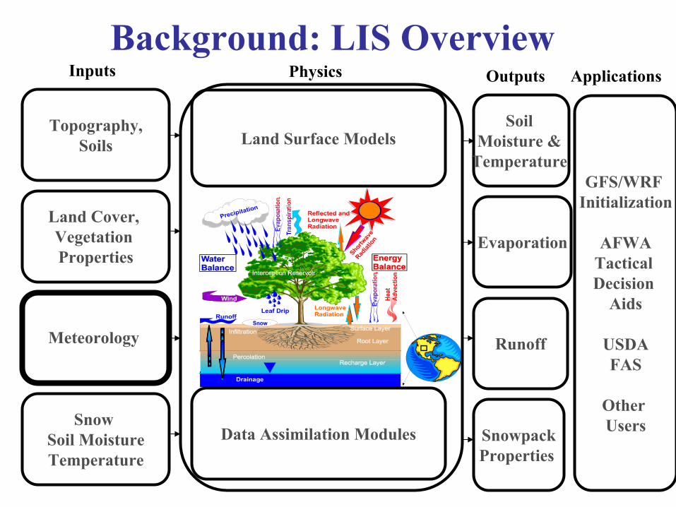
Topography,Soils
Land Cover, Vegetation Properties
Meteorology
Snow Soil MoistureTemperature
Land Surface Models
Data Assimilation Modules
Soil Moisture &
Temperature
Evaporation
Runoff
SnowpackProperties
Inputs OutputsPhysics
GFS/WRF Initialization
AFWATactical Decision
Aids
USDAFAS
Other Users
Applications
Background: LIS Overview
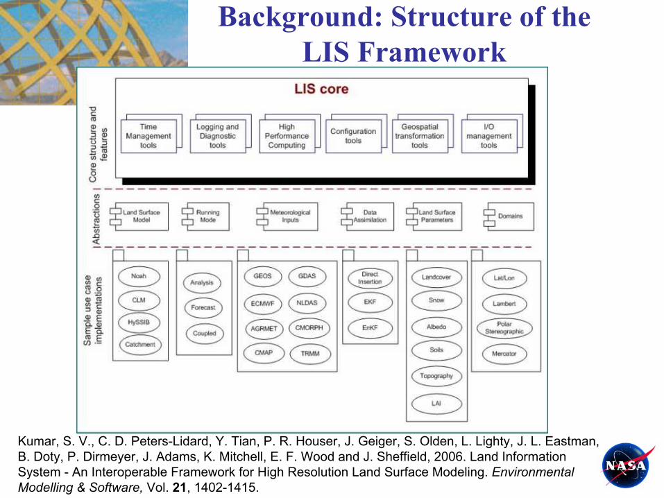
Background: Structure of the LIS Framework
Kumar, S. V., C. D. Peters-Lidard, Y. Tian, P. R. Houser, J. Geiger, S. Olden, L. Lighty, J. L. Eastman, B. Doty, P. Dirmeyer, J. Adams, K. Mitchell, E. F. Wood and J. Sheffield, 2006. Land Information System - An Interoperable Framework for High Resolution Land Surface Modeling. Environmental Modelling & Software, Vol. 21, 1402-1415.
Outline
1. Integrating NASA/GMAO’s EnKF in LIS2. Coupling LIS to NOAA/NEMS3. Coupling LIS to JCSDA/CRTM4. Coupling LIS to WRF/ARW
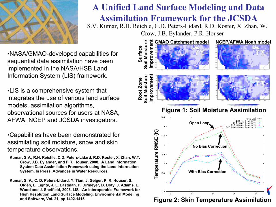
A Unified Land Surface Modeling and Data Assimilation Framework for the JCSDA
•NASA/GMAO-developed capabilities for sequential data assimilation have been implemented in the NASA/HSB Land Information System (LIS) framework.
•LIS is a comprehensive system that integrates the use of various land surface models, assimilation algorithms, observational sources for users at NASA, AFWA, NCEP and JCSDA investigators.
•Capabilities have been demonstrated for assimilating soil moisture, snow and skin temperature observations.
Crow, J.B. Eylander, and P.R. Houser, 2008. A Land Information System Data Assimilation Framework using the Land Information System, In Press, Advances in Water Resources.
Kumar, S. V., C. D. Peters-Lidard, Y. Tian, J. Geiger, P. R. Houser, S. Olden, L. Lighty, J. L. Eastman, P. Dirmeyer, B. Doty, J. Adams, E. Wood and J. Sheffield, 2006. LIS - An Interoperable Framework for High Resolution Land Surface Modeling. Environmental Modeling and Software, Vol. 21, pp 1402-1415.
Tem
pera
ture
RM
SE (K
)
Open Loop
With Bias Correction
No Bias Correction
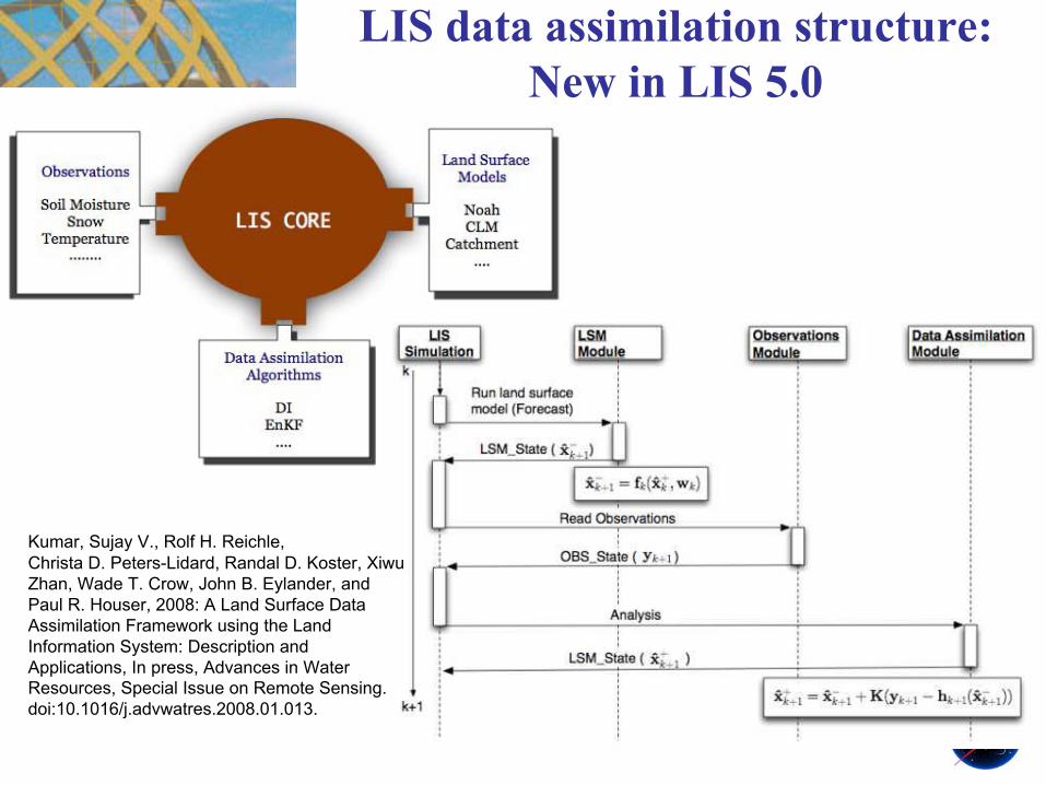
Kumar, Sujay V., Rolf H. Reichle,Christa D. Peters-Lidard, Randal D. Koster, Xiwu Zhan, Wade T. Crow, John B. Eylander, and Paul R. Houser, 2008: A Land Surface Data Assimilation Framework using the Land Information System: Description and Applications, In press, Advances in Water Resources, Special Issue on Remote Sensing.doi:10.1016/j.advwatres.2008.01.013.
LIS data assimilation structure: New in LIS 5.0
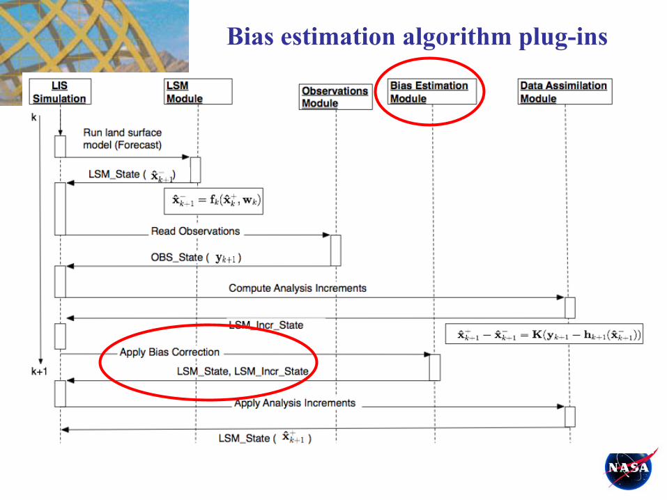
Bias estimation algorithm plug-ins
Bias estimation approaches in LIS
1. Off-line (a priori) scaling between climatology of obs. and land model:+ No assumption whether model or observations are biased.+ Easy to implement in pre-processing.− Static (cannot adjust to changes in bias).
2. Dynamic model bias estimation:− Assume obs. climatology is correct and the model is biased.+ Dynamic (adjusts to changes in bias).
Kb = function(Kx)Use KF increments to update bias.Bias estimate is effectively time average of increments.Options for diurnal and semi-diurnal biasparameterization.
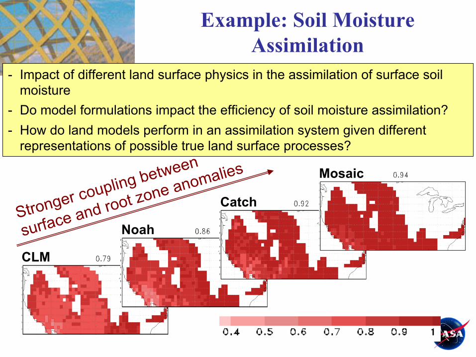
Example: Soil Moisture Assimilation
- Impact of different land surface physics in the assimilation of surface soil moisture
- Do model formulations impact the efficiency of soil moisture assimilation?- How do land models perform in an assimilation system given different
representations of possible true land surface processes?
CLM
Noah
Catch
Mosaic
Stronger coupling between
surface and root zone anomalies
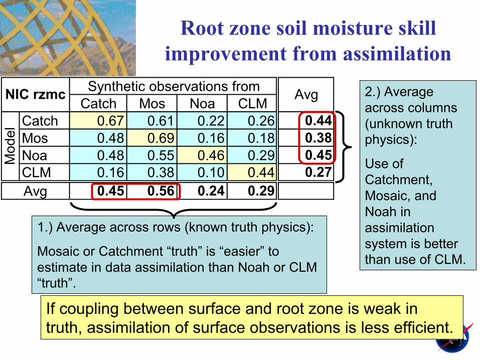
Root zone soil moisture skill improvement from assimilation
1.) Average across rows (known truth physics):
Mosaic or Catchment “truth” is “easier” to estimate in data assimilation than Noah or CLM “truth”.
2.) Average across columns (unknown truth physics):
Use of Catchment, Mosaic, and Noah in assimilation system is better than use of CLM.
If coupling between surface and root zone is weak in truth, assimilation of surface observations is less efficient.
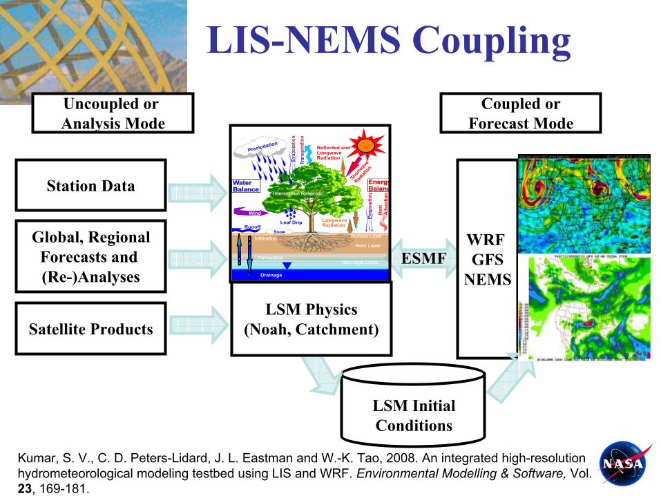
Kumar, S. V., C. D. Peters-Lidard, J. L. Eastman and W.-K. Tao, 2008. An integrated high-resolution hydrometeorological modeling testbed using LIS and WRF. Environmental Modelling & Software, Vol. 23, 169-181.
LIS-NEMS interface
• Land runs on the same grid as the atmosphere• Static initializations and parameters in the input
interface
14
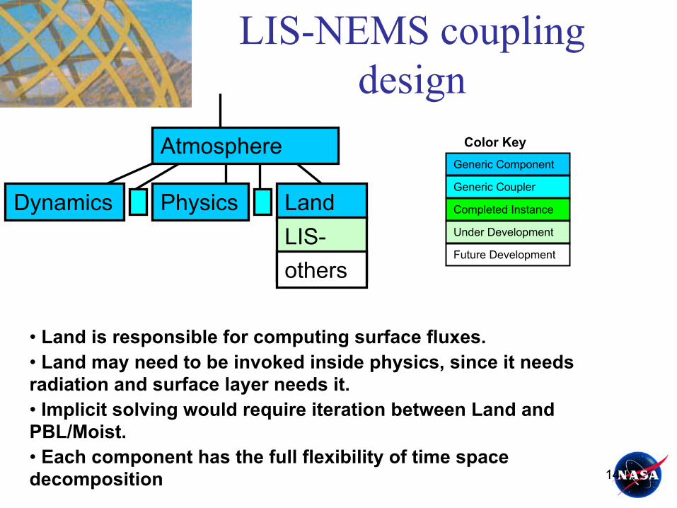
LIS-NEMS coupling design
Color KeyGeneric Component
Generic Coupler
Completed Instance
Under Development
Future Development
• Land is responsible for computing surface fluxes.• Land may need to be invoked inside physics, since it needs radiation and surface layer needs it.• Implicit solving would require iteration between Land and PBL/Moist.• Each component has the full flexibility of time space decomposition
Dynamics Physics LandLIS-Noahothers
Atmosphere
GFS Computational Scaling(T62)
• 6days starting 25 jul2007, using a timestepof 600sec, 3 hourly output
• T62 test case was run for several different tasks/nodes combinations.
• These timing results will allow us to measure the impact of coupling GFS and LIS.
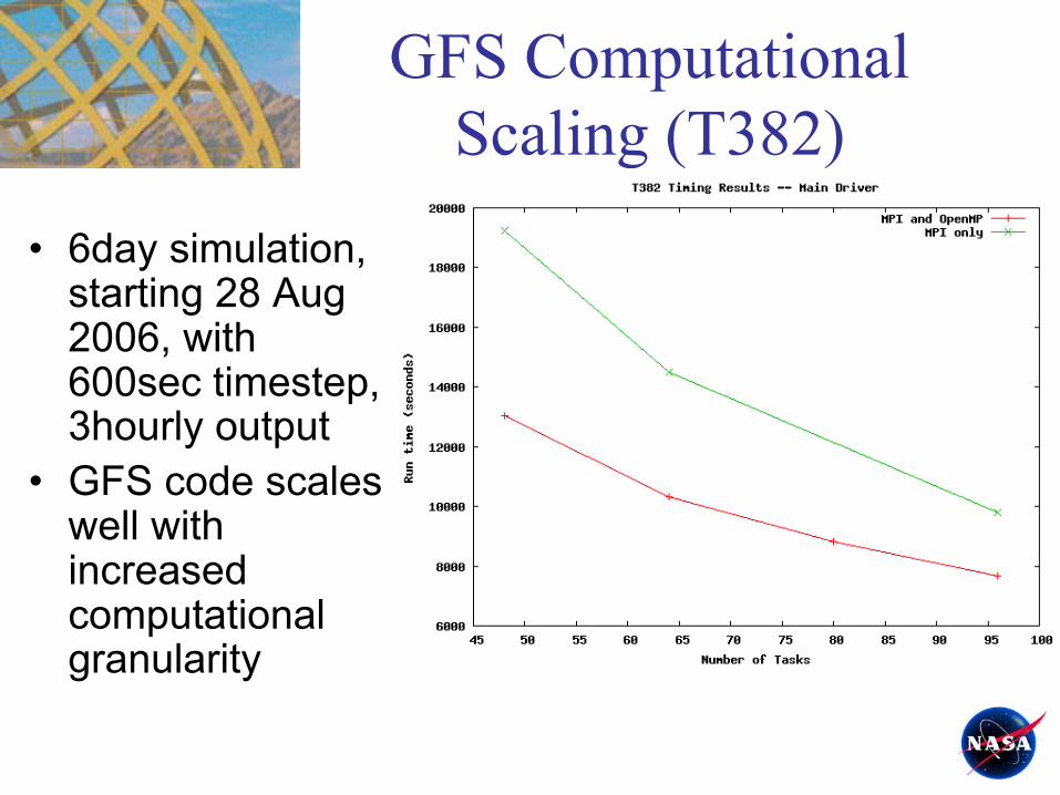
GFS Computational Scaling (T382)
• 6day simulation, starting 28 Aug 2006, with 600sec timestep, 3hourly output
• GFS code scales well with increased computational granularity
LIS-NEMS Coupling Progress
• LIS version 5.0 has been benchmarked on the JCSDA testbed (haze)
• A number of design prototypes for the LIS-NEMS coupling have been developed
• The domain decomposition strategies from NEMS have been abstracted
• A direct coupling strategy for combining LIS and NEMS is being explored.
• Test case: September, 2007– Control: AGRMET– CRTM Four-stream Fu-Liou
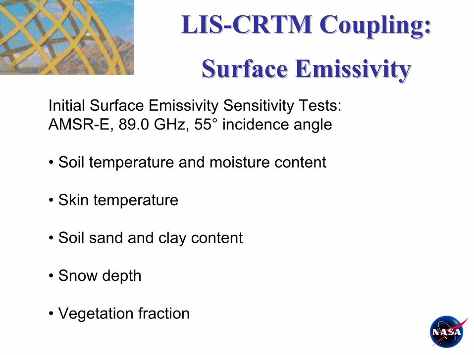
LISLIS--CRTM CouplingCRTM Coupling
Atmospheric RTAtmospheric RT
AFWA simulation in the clear sky condition is close to truth, but in cloudy or partly cloudy conditions the AFWA simulation overestimated or underestimated the flux.
Partlycloudy
Partlycloudy
Cloudy Clear sky
Penn State, PA
Goodwin Creek, MS
Sioux Falls, SD
Bondville, IL
AGRMET vs. LISAGRMET vs. LIS--CRTM CRTM Downward SWDownward SW
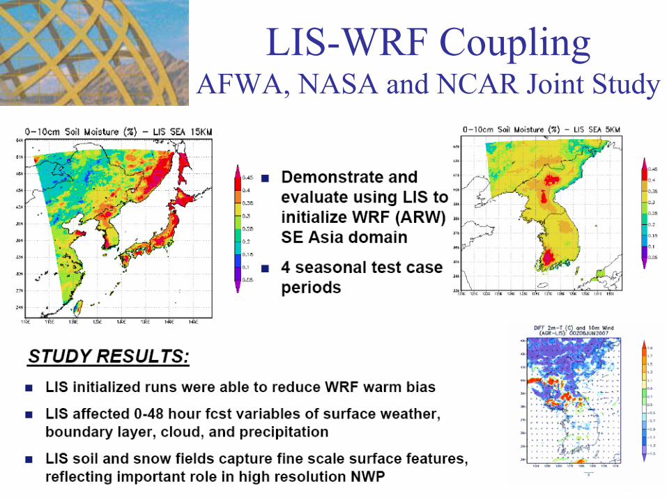
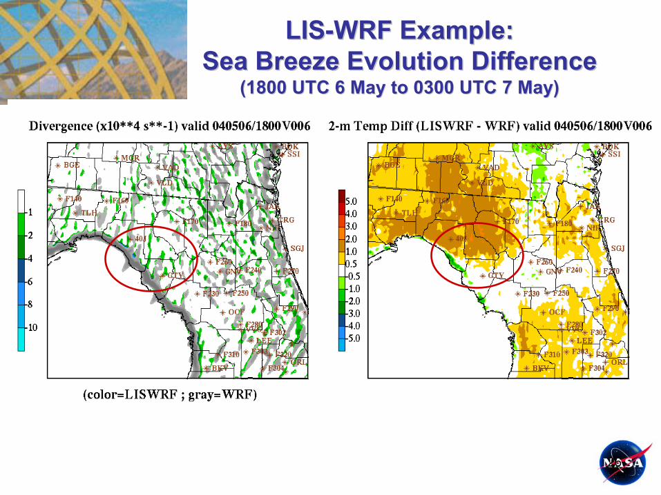
LIS-WRF CouplingAFWA, NASA and NCAR Joint Study
25
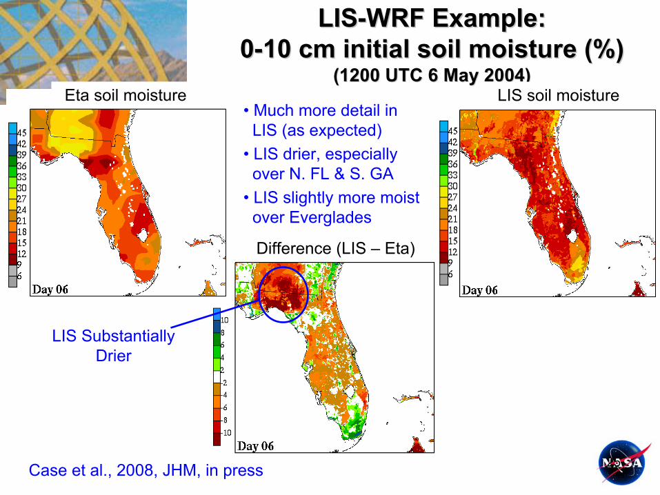
LISLIS--WRF Example:WRF Example:00--10 cm initial soil moisture (%)10 cm initial soil moisture (%)
(1200 UTC 6 May 2004)(1200 UTC 6 May 2004)Eta soil moisture LIS soil moisture
((MeteogramMeteogram plots at 40J and CTY)plots at 40J and CTY)
Summary1. We have successfully integrated NASA/GMAO’s
EnKF in LIS for use by JCSDA investigators2. With NCEP/UMIG, we have designed the interface for
coupling LIS to NOAA/NEMS and completed uncoupled benchmarks
3. With NCEP, AFWA and NESDIS, we are working towards coupling LIS to JCSDA/CRTM, with a focus on MW, VIS, IR.
4. With NCAR and AFWA, we have coupled LIS to WRF/ARW, and we will streamline this coupling to be ESMF compliant and ready “out of the box”.
Backup
30
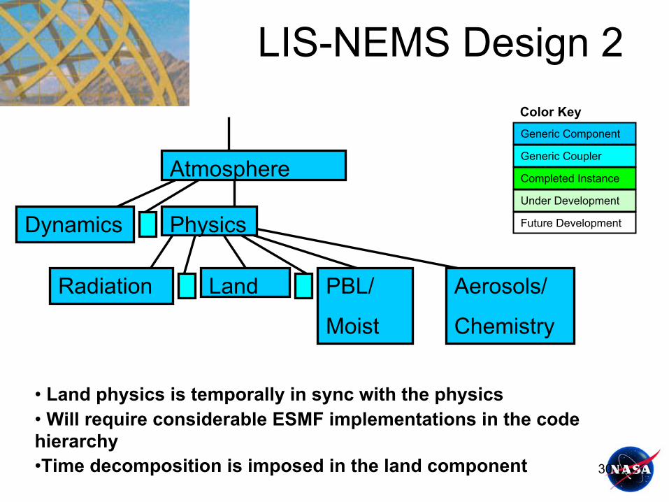
LIS-NEMS Design 2Color KeyGeneric Component
Generic Coupler
Completed Instance
Under Development
Future Development
• Land physics is temporally in sync with the physics• Will require considerable ESMF implementations in the code hierarchy•Time decomposition is imposed in the land component