1 Progress Report 4: October 1, 2010 – March 31, 2011 Accessing Brownfield Sustainability: Lifecycle Assessment and Carbon Footprinting The Western Pennsylvania Brownfields Center at Carnegie Mellon, in collaboration with the Pennsylvania Downtown Center US Environmental Protection Agency Brownfield Training Research and Technical Assistance Grant Award: TR – 83417301 – 0 May 6, 2011 A. Background The primary purpose of this project is to develop the methodology and subsequent tools that stakeholders can use to assess the sustainability of Brownfield development as measured through carbon footprinting, pollutant emissions and energy impacts. The research is intended to apply innovative analytical techniques (such as economic input-output life cycle analysis) to estimate the carbon emissions, pollutant emissions and energy impacts associated with Brownfield development; while documenting the drivers of these impacts given alternative Brownfield development scenarios. Training and technical assistance efforts complement the primary research purpose. Through training, we intend to educate and disseminate information that will allow the members of the community to better understand the public health risks of unattended Brownfields and the benefits of alternative remediation strategies. Through technical assistance, we intend to provide targeted communities with a prioritization tool that will allow for fair, transparent and equitable Brownfield development decisions. Our work has been divided into 3 primary Activities: • Activity 1: Training – Empowerment Through Knowledge. Enhance Pennsylvania Downtown Center’s (PDC) webpage for Brownfield relevant information, participate in annual PDC events to provide Brownfield related content, and conduct topic specific seminars. As the
Transcript
1
Progress Report 4: October 1, 2010 – March 31, 2011 Accessing Brownfield Sustainability: Lifecycle Assessment and Carbon Footprinting
The Western Pennsylvania Brownfields Center at Carnegie Mellon, in collaboration with the Pennsylvania Downtown Center
US Environmental Protection Agency Brownfield Training Research and Technical Assistance Grant
Award: TR – 83417301 – 0 May 6, 2011
A. Background The primary purpose of this project is to develop the methodology and subsequent tools that
stakeholders can use to assess the sustainability of Brownfield development as measured through
carbon footprinting, pollutant emissions and energy impacts. The research is intended to apply
innovative analytical techniques (such as economic input-output life cycle analysis) to estimate
the carbon emissions, pollutant emissions and energy impacts associated with Brownfield
development; while documenting the drivers of these impacts given alternative Brownfield
development scenarios.
Training and technical assistance efforts complement the primary research purpose. Through
training, we intend to educate and disseminate information that will allow the members of the
community to better understand the public health risks of unattended Brownfields and the
benefits of alternative remediation strategies. Through technical assistance, we intend to provide
targeted communities with a prioritization tool that will allow for fair, transparent and equitable
Brownfield development decisions.
Our work has been divided into 3 primary Activities:
• Activity 1: Training – Empowerment Through Knowledge. Enhance Pennsylvania Downtown
Center’s (PDC) webpage for Brownfield relevant information, participate in annual PDC
events to provide Brownfield related content, and conduct topic specific seminars. As the
2
project proceeds, the target group for training will be expanded beyond PDC’s current
membership.
• Activity 2: Research – Quantifying the Sustainable Brownfield. Develop a life cycle
assessment model, including footprinting, for comparison of Brownfield development relative
to greenfield development, beta test the tool on sites (preferably) selected in cooperation with
PDC members, finalize and validate the model, develop a computer based tool, train PDC
members to use the tool, and coordinate with US Environmental Protection Agency to develop
strategy for transferring tool to other Brownfield stakeholders.
• Activity 3: Technical Assistance – Site Selection Through Prioritization. Assist PDC members
in developing inventories of sites, beta test the Site Prioritization tool with select PDC
members, finalize Site Prioritization tool, distribute Tool to remainder of PDC members, and
coordinate with the Pennsylvania Department of Environmental Protections and the USEPA to
develop strategy for transferring both tools to other Brownfield stakeholders.
B. Overall Progress
The official date of the award was March 12, 2009. Pre-award approval from the USEPA Project
Officer allowed our work to commence in October 2008 and our first Progress Report was
submitted on October 1, 2009. Progress Report 2 addressed the time period between October
2009 and March 2010. Progress Report 3 addressed the time period between April 1 and
September 30, 2010. And, Progress Report 4 addresses the time period between October 1, 2010
and March 31, 2011.
Carnegie Mellon personnel working on technical aspects of the project during Period 4 include
Professor Chris Hendrickson, Dr. Deborah Lange, and graduate students Amy Nagengast and
Yeganeh Mashayekh. PDC personnel working on the project include Bill Fontana and Eddy
Kaplaniak; as well as members of the Keystone CORE Services group.
3
Overall progress with respect to each Activity is summarized as follows:
Activity 1: Training – Empowerment Through Knowledge – we continue to participate in PDC
meetings and have shared information with the equivalent of more than 96 communities in
Pennsylvania. PDC’s brownfield webpage is available at:
• Community Revitalization Academy, Community Marketing - 11/16-17 - 19 people
WEBSITE
PDC, working with CMU, will continue to add content including videos, progress reports, and
educational opportunities, to the Brownfield area of the site. The website will also track the
community-initiated feasibility pilot program, which will include a data base of possible small
site Brownfields.
Activity 2: Research – Quantifying the Sustainable Brownfield We are pursuing three sub-activities within Activity 2. In Activity 2A, we are making site
specific comparisons between a local brownfield and greenfield development. In Activity 2B,
we are looking at census data gathered in year 2000 to evaluate the commuting behavior of
people living in census tracts that contain brownfield development as compared to census tracks
that contain greenfield developments. In Activity 2C, we are evaluating all vehicular
transportation of residents for a number of brownfield/greenfield pairs using regional travel
demand models. Beyond transportation analyses, we will begin to gather and analyze data on
water and electricity usage.
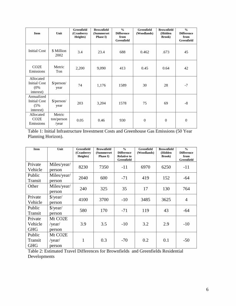
Activity 2A: Site Specific Comparisons
Completed during this period we analyzed two additional residential case studies: Hidden Brook
(brownfield) and The Woodlands (greenfield); both residential developments in Peters Township
(located about 20 miles south of Pittsburgh, PA.) The developments are about 5 miles apart.
With all costs are adjusted to 2002 values, the PRELIMINARY results for all 4 case studies are
summarized in the following tables:
6
Item
Unit
Greenfield (Cranberry
Heights)
Brownfield (Summerset
Phase I)
% Difference
from Greenfield
Greenfield (Woodlands)
Brownfield (Hidden Brook)
% Difference
from Greenfield
Initial Cost
$ Million
2002 3.4 23.4 688 0.462 .673 45
CO2E
Emissions
Metric
Ton 2,200 9,090 413 0.45 0.64 42
Allocated Initial Cost
(0% interest)
$/person/
year 74 1,176 1589 30 28 -7
Annualized Initial Cost
(5% interest)
$/person/
year 203 3,204 1578 75 69 -8
Allocated CO2E
Emissions
Metric ton/person
/year 0.05 0.46 930 0 0 0
Table 1: Initial Infrastructure Investment Costs and Greenhouse Gas Emissions (50 Year Planning Horizon).
Item Unit Greenfield (Cranberry
Heights)
Brownfield (Summerset
Phase I)
% Difference Relative to Greenfield
Greenfield (Woodlands)
Brownfield (Hidden Brook)
% Difference
from Greenfield
Private Vehicle
Miles/year/person 8230 7350 -11 6970 6250 -11
Public Transit
Miles/year/person 2040 600 -71 419 152 -64
Other Miles/year/person 240 325 35 17 130 764
Private Vehicle
$/year/ person 4100 3700 -10 3485 3625 4
Public Transit
$/year/ person 580 170 -71 119 43 -64
Private Vehicle GHG
Mt CO2E /year/ person
3.9 3.5 -10 3.2 2.9 -10
Public Transit GHG
Mt CO2E /year/ person
1 0.3 -70 0.2 0.1 -50
Table 2: Estimated Travel Differences for Brownfields and Greenfields Residential Developments
7
Item Unit Greenfield (Cranberry Heights)
Brownfield (Summerset Phase I)
% Difference Relative to Greenfield
Greenfield (Woodlands)
Brownfield (Hidden Brook)
% Difference from Greenfield
Average Floor Space
Sq. ft./ residence 2,700 2,460 -9 2800 2800 0
Land Area Acres/ residence 1.1 0.16 -85 .50 0.44 -12
Natural Gas (monthly)
$/residence 170 89 -52 136 83 -39
Electricity (monthly)
$/residence 133 94 -29 103 57 -45
Water/ Sewer (monthly)
$/residence 79 27 -66 62 41 -34
Total Utilities (monthly)
$/residence 382 210 -45 301 181 -40
Total Utilities
$/person 103 105 3 97 75 -23
Floor Space Sq. ft./ person 730 1,230 68 903 1167 29
Developm’t Area
Acres/ person 0.3 0.08 -73 0.13 0.18 38
Building Construction GHG
Metric ton 61,400 30,909 -50 11.8 24.5 107
Allocated Building Construction GHG
Metric ton/ person/year 1.3 1.5 15 0 .05 --
Utility GHG Metric ton/person/year
5.9 9.6 63 8.6 6.4 -26
Table 3: Residential Building Differences
Given the 4 case analyses that have been conducted the following observations can be made:
• With respect to construction, the emissions associated with housing construction are much
greater than emission associated with site development.
• With respect to ‘use,’ emissions associated with utility consumption outweigh those
associated with transportation.
• Overall (and over a given planning horizon), emissions associated with the ‘use’ phase
greatly exceed those of the construction phase.
8
In addition to the case analyses, we have been working in parallel to develop a methodology that
allows the preparation of case analyses by the acquisition of publicly available information and
with out the burden of residential surveys and visits to the municipal engineer. We will revisit
this effort during the summer of 2011.
Activity 2B – Commuting Behavior of Residents The commuting behavior of residents in brownfield and greenfield neighborhoods within six
cities was accomplished using the 2000 US Decennial Census and supplemental external data.
This research has been completed and is awaiting final publication for the ASCE Journal of
Urban Planning and Development. Furthermore, an abstract from this research was submitted
and accepted for an oral presentation at the Engineering Sustainability 2011: Innovation and the
Triple Bottom Line Conference April 10-12 in Pittsburgh, PA. During this reporting period,
presentation slides have been completed for this talk to be given by Amy Nagengast.
Activity 2C – Yeganeh Mashayekh, a graduate student in Civil and Environmental Engineering
and Engineering and Public Policy at Carnegie Mellon is planning her PhD studies around this
topic. She successfully passed her Engineering and Public Policy qualifying examination
presenting her work on this topic:
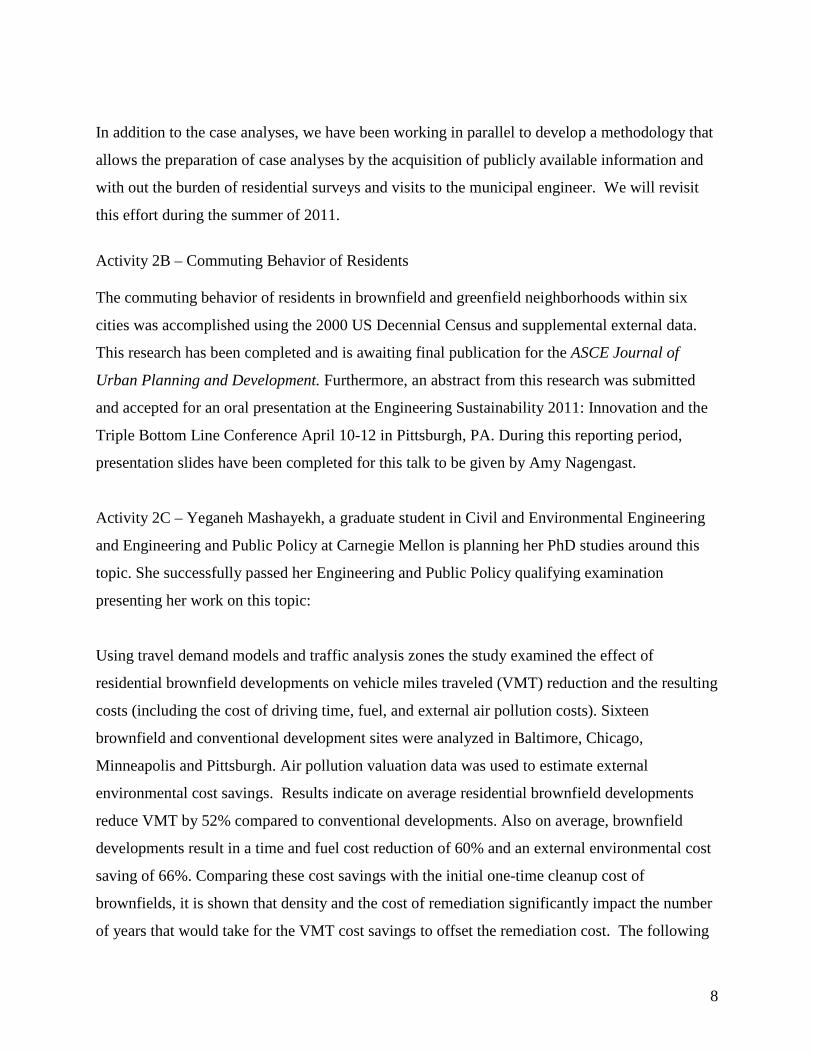
Using travel demand models and traffic analysis zones the study examined the effect of
residential brownfield developments on vehicle miles traveled (VMT) reduction and the resulting
costs (including the cost of driving time, fuel, and external air pollution costs). Sixteen
brownfield and conventional development sites were analyzed in Baltimore, Chicago,
Minneapolis and Pittsburgh. Air pollution valuation data was used to estimate external
environmental cost savings. Results indicate on average residential brownfield developments
reduce VMT by 52% compared to conventional developments. Also on average, brownfield
developments result in a time and fuel cost reduction of 60% and an external environmental cost
saving of 66%. Comparing these cost savings with the initial one-time cleanup cost of
brownfields, it is shown that density and the cost of remediation significantly impact the number
of years that would take for the VMT cost savings to offset the remediation cost. The following
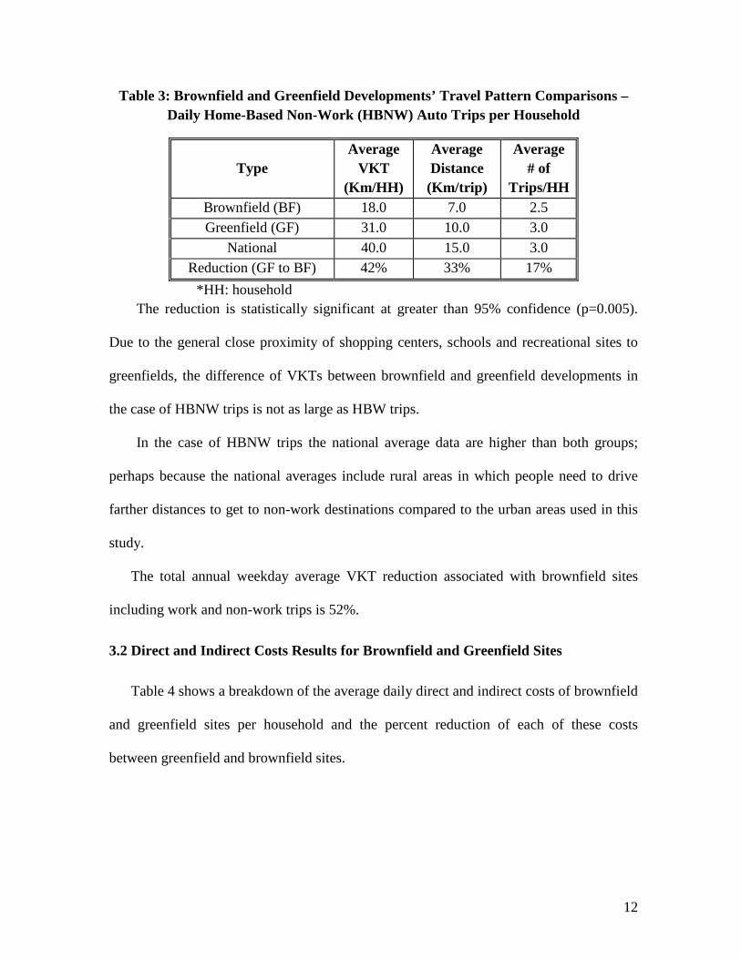
9
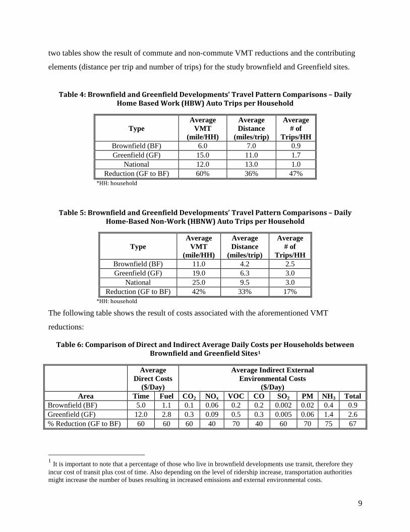
two tables show the result of commute and non-commute VMT reductions and the contributing
elements (distance per trip and number of trips) for the study brownfield and Greenfield sites.
Table 4: Brownfield and Greenfield Developments’ Travel Pattern Comparisons – Daily Home Based Work (HBW) Auto Trips per Household
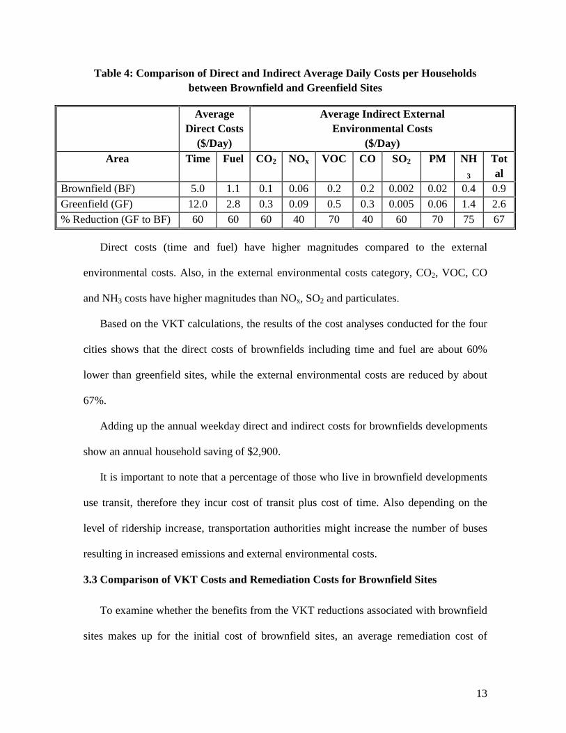
1 It is important to note that a percentage of those who live in brownfield developments use transit, therefore they incur cost of transit plus cost of time. Also depending on the level of ridership increase, transportation authorities might increase the number of buses resulting in increased emissions and external environmental costs.
10
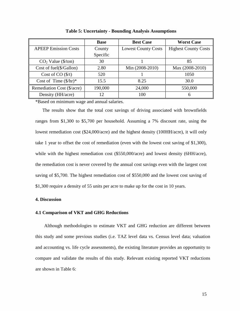
The study furthermore compared the VMT reduction cost savings with the initial cost of
remediation. It turned out that the technology used for remediation and the density of
developments has a significant impact on the breakeven point between the VMT reduction cost
saving and the cost of remediation.
In addition the study compared brownfield developments as a strategy to reduce VMT with other
conventional VMT reduction strategies (i.e. carpooling, congestion pricing). The result shows
that brownfield developments can be used as a cost effective strategy method to reduce VMT; in
comparison to other VMT reduction strategies, brownfield developments have minimal cost to
transportation authorities and the benefits are comparable with other strategies. Therefore, it is
recommended that public agencies including and not limited to USEPA and US Department of
Transportation work collaboratively to choose sites that would optimize remediation cost and
travel and environmental cost savings.
A paper (Appendix A) on this research has been submitted to Journal of Urban Planning and
Development, American Society of Civil Engineers.
Additional Activities:
- As part of activity 2C, a preliminary study was originally conducted using the same
methodology of pollution valuation to measure the environmental cost of traffic
congestion in about ninety U.S. metropolitan areas. This study was presented last
January (2011) in the 90th annual Transportation Research Board conference in
Washington D.C. The paper (Appendix B) has been accepted to be published in
Transportation Research Records (TRR) during the Spring of 2011.
- During the 14th National Brownfield Conference cosponsored by EPA, we
participated in a panel discussion named “Partnership 101: Working with
Universities”. Yeganeh Mashayekh from Carnegie Mellon/Western Pennsylvania
Brownfields Center was on the panel. Each panelist discussed what they do and
what the challenges are. Through an interactive discussion with the audience the
11
panel was able to identify some of the issues related to partnership with universities
and discuss some potential solutions.
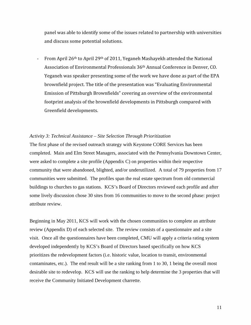
- From April 26th to April 29th of 2011, Yeganeh Mashayekh attended the National
Association of Environmental Professionals 36th Annual Conference in Denver, CO.
Yeganeh was speaker presenting some of the work we have done as part of the EPA
brownfield project. The title of the presentation was “Evaluating Environmental
Emission of Pittsburgh Brownfields” covering an overview of the environmental
footprint analysis of the brownfield developments in Pittsburgh compared with
Greenfield developments.
Activity 3: Technical Assistance – Site Selection Through Prioritization
The first phase of the revised outreach strategy with Keystone CORE Services has been
completed. Main and Elm Street Managers, associated with the Pennsylvania Downtown Center,
were asked to complete a site profile (Appendix C) on properties within their respective
community that were abandoned, blighted, and/or underutilized. A total of 79 properties from 17
communities were submitted. The profiles span the real estate spectrum from old commercial
buildings to churches to gas stations. KCS’s Board of Directors reviewed each profile and after
some lively discussion chose 30 sites from 16 communities to move to the second phase: project
attribute review.
Beginning in May 2011, KCS will work with the chosen communities to complete an attribute
review (Appendix D) of each selected site. The review consists of a questionnaire and a site
visit. Once all the questionnaires have been completed, CMU will apply a criteria rating system
developed independently by KCS’s Board of Directors based specifically on how KCS
prioritizes the redevelopment factors (i.e. historic value, location to transit, environmental
contaminates, etc.). The end result will be a site ranking from 1 to 30, 1 being the overall most
desirable site to redevelop. KCS will use the ranking to help determine the 3 properties that will
receive the Community Initiated Development charrette.
12
Action Steps
1) Communities interested in assistance from Keystone C.O.R.E. Services will have to first
complete a site inventory of abandoned, blighted, underutilized properties. Communities can
submit as many properties as they would like that meet the criteria. Completed: 79
Properties were submitted.
2) From the submitted sites, PDC will chose 30 sites (the intent is that the 30 sites will be in 30
DIFFERENT communities) to move to the next level of evaluation. Completed: February
2011.
3) Working closely with PDC staff, the 30 chosen communities will complete a site attribute
profile for each of the sites selected. Site visits are scheduled for May and June 2011.
4) While the site attributed profiles are being completed KCS’s board of directors will work
with CMU to weight the criteria. Scheduled for May 9,, 2011.
5) CMU will combine the completed site attribute profiles with the criteria weighting system.
Date TBD
6) KCS’s board of directors will choose 3 sites (from the weighted 30) to undertake a
community initiated feasibility study. KCS intends on using 3rd and 4th year college interns to
help facilitate the data collection on the 3 sites. Dates TBD.
Timeline
• Oct Nov Dec 2010 - Communities complete site inventory.
• Jan 2011 - PDC chooses 30 sites from site inventory list to move to the next stage – site
attribute profile.
• Feb 2, 2011 – PDC chooses 20 sites from the site inventory list to move to the next
• Mach April May 2011 - PDC works with the 30 communities to complete the site attribute
profile.
• May 2, 2011 – KCS’s board works with CMU to weight the criteria.
• May 2011 - CMU applies criteria to the attribute profiles.
• June 6, 2011 - Keystone C.O.R.E Services chooses three (3) communities to move to the
next stage – site feasibility analysis
• June July Aug 2011 - Interns gather site specific feasibility information on each site.
13
• Sept 2011 - KCS conducts its first taskforce visit to complete a community driven
feasibility study.
• Oct 2011- KCS conducts its second taskforce visit to complete a community driven
feasibility study.
• Nov 2011 - KCS conducts its third taskforce visit to complete a community driven
feasibility study.
D. Progress vs Proposed Milestones The proposed milestones for Years 1, 2 and 3 are presented in our application package are
summarized in the following table. Note that this report is intended to summarize the first 6
months of Year 3, however, our Year 3 funding has not yet been authorized by the USEPA.
Completion YEAR
Activity 1: Training – Empowerment through Knowledge
Activity 2: Research – Quantifying a Sustainable Brownfield
Activity 3: Technical Assistance – Site Selection through Prioritization
1 .Participate in PDC regional events .Update PDC webpage with Brownfield related content .Nat’l Brownfields Conference (Fall 2009)
Develop framework and scope for life cycle assessment and carbon footprinting tool
Complete inventories in select Main Street/ Elm Street Communities
2 As above with webpage updates including additional case studies
Finalize transportation, building, electricity and water analysis modules
Initiate ranking process select Main Street/ Elm Street Communities
3 As above with webpage updates including additional case studies .Nat’l Brownfields Conference (Spring 2011)
Demonstrate, troubleshoot and validate model and tool
Complete ranking process select Main Street/ Elm Street Communities
Our progress to date (through the first 6 months of Year 3) can be summarized as follows:
Activity 1: We are on track and working with PDC is their regional events. PDC webpage is
active and we will need to focus on assuring the accuracy of the information on the webpage and
adding case studies. (In addition, we will continue to add case studies to the webpage hosted by
the Western Pennsylvania Brownfields Center: www.cmu.edu.steinbrenner/brownfields)
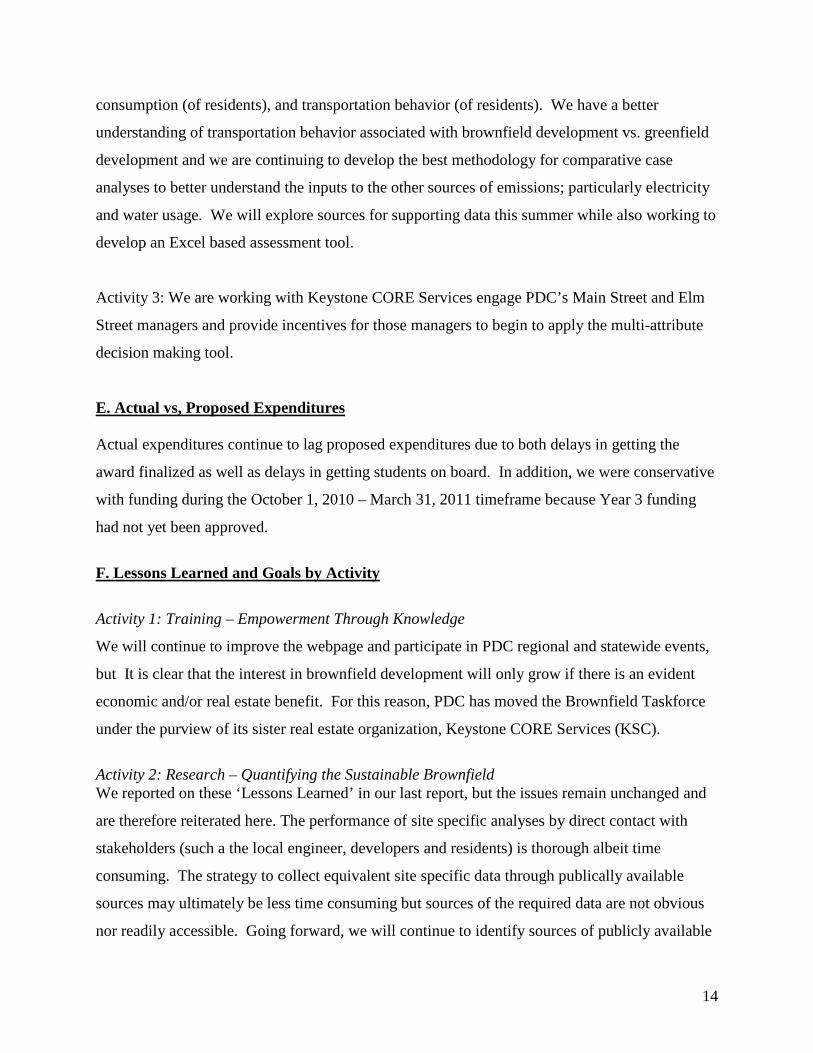
Activity 2: We continue to look for publicly available sources of data that can be used to
understand environmental emissions: remediation, site preparation, housing construction, utility
14
consumption (of residents), and transportation behavior (of residents). We have a better
understanding of transportation behavior associated with brownfield development vs. greenfield
development and we are continuing to develop the best methodology for comparative case
analyses to better understand the inputs to the other sources of emissions; particularly electricity
and water usage. We will explore sources for supporting data this summer while also working to
develop an Excel based assessment tool.
Activity 3: We are working with Keystone CORE Services engage PDC’s Main Street and Elm
Street managers and provide incentives for those managers to begin to apply the multi-attribute
decision making tool.
E. Actual vs, Proposed Expenditures Actual expenditures continue to lag proposed expenditures due to both delays in getting the
award finalized as well as delays in getting students on board. In addition, we were conservative
with funding during the October 1, 2010 – March 31, 2011 timeframe because Year 3 funding
had not yet been approved.
F. Lessons Learned and Goals by Activity
Activity 1: Training – Empowerment Through Knowledge
We will continue to improve the webpage and participate in PDC regional and statewide events,
but It is clear that the interest in brownfield development will only grow if there is an evident
economic and/or real estate benefit. For this reason, PDC has moved the Brownfield Taskforce
under the purview of its sister real estate organization, Keystone CORE Services (KSC).
Activity 2: Research – Quantifying the Sustainable Brownfield We reported on these ‘Lessons Learned’ in our last report, but the issues remain unchanged and
are therefore reiterated here. The performance of site specific analyses by direct contact with
stakeholders (such a the local engineer, developers and residents) is thorough albeit time
consuming. The strategy to collect equivalent site specific data through publically available
sources may ultimately be less time consuming but sources of the required data are not obvious
nor readily accessible. Going forward, we will continue to identify sources of publicly available
15
data so that we can prepare additional site analyses. To date, we have performed 2-pairs (or 4)
site analyses. Results are somewhat consistent in suggesting the environmental emissions from
the ‘operating’ portion of the development (ie residential behavior on a brownfield or a
greenfield development) greatly exceed the emissions that result from the combination of
remediation and construction activities. We will continue to prepare additional analyses, via
direct and indirect communications and data collection, to further understand this potential
trending.
We have successfully found data for the transportation analyses part of this effort. Going
forward, we will be looking at the electricity and water usage analyses.
Activity 3: Technical Assistance – Site Selection Through Prioritization
We will focus our efforts on working with PDC to implementing an alternative approach to reach
these communities within the Main Street and Elm Street Programs. Again, interest and
participation will be based on incentives that can be generated through the Keystone CORE
Services group of PDC.
We note that Progress Report 5 will include efforts performed between April 1, 2011 and
September 30, 2011.
Respectfully submitted,
, Executive Director Steinbrenner Institute and the Western Pennsylvania Brownfields Center [email protected] (412) 268-7121
The Role of Brownfield Developments in Reducing Household Vehicle Travel
Yeganeh Mashayekh2, Chris Hendrickson3 Hon. M. ASCE, and H. Scott Matthews A.M.ASCE 4
Abstract
The transportation sector is the second largest source of GHG emissions in the U.S.
Reviving underutilized industrial sites can reduce the transportation sector’s impact on the
environment by lowering vehicle kilometers traveled (VKT).
This study examines the effect of residential brownfield developments on VKT
reduction and the resulting costs (including the cost of driving time, fuel, and external air
pollution costs). Sixteen brownfield and conventional development sites were analyzed in
Baltimore, Chicago, Minneapolis and Pittsburgh. Travel demand models were used to
estimate VKT reductions. Air pollution valuation data was used to estimate external
environmental cost savings. Results indicate on average residential brownfield
developments reduce VKT by 52% compared to conventional developments. Also on
average, brownfield developments result in a time and fuel cost reduction of 60% and an
external environmental cost saving of 66%. Comparing these cost savings with the initial
one-time cleanup cost of brownfields, it is shown that density and the cost of remediation
significantly impact the number of years that would take for the VKT cost savings to
offset the remediation cost. 2 Research Assistant, Department of Civil & Environmental Engineering, Department of Engineering & Public Policy, Carnegie Mellon University, Pittsburgh, PA 15213-3890 3 Professor, Department of Civil & Environmental Engineering, Carnegie Mellon University, Pittsburgh, PA 15213-3890 4 Professor, Department of Civil & Environmental Engineering and Department of Engineering & Public Policy, Carnegie Mellon University, Pittsburgh, PA 15213-3890
1
Subject Headings
Remediation, Industrial Facilities, Vehicles, Air Pollution, Environmental Issues,
Brownfields, Vehicle Kilometers Traveled
1. Introduction
Brownfields are properties for which expansion, redevelopment, or reuse may be
complicated by the presence or potential presence of hazardous substances, pollutants, or
contaminants (EPA 2009). An estimated 450,000 to 1,000,000 brownfield sites remain
abandoned across the country (US GAO 2004). These sites include former industrial or
manufacturing plants, dry cleaners, gas stations, laboratories and residential buildings.
Developing brownfields incurs initial assessment and remediation costs and involves
barriers such as uncertainty about the presence and type of contamination, uncertainty
over cleanup standards, limited cleanup resources, and potential liability issues (HUD
2010; OTA 1995). On the other hand, developing these underutilized lands can positively
impact economic development and the environment (Lange 2004). Brownfield
developments have been shown to revive communities (Kaufman 2006), increase
employment (De Sousa 2005), generate local tax revenue (De Sousa 2005), and keep
green spaces intact (GWU 2001)
To make a proper decision about developing a brownfield site, it is important that all
benefits and costs are taken into account. In this paper, we analyze the impact of
residential brownfield developments on travel activity reduction and the consequential
costs including the cost of time and fuel as well as the external environmental costs.
2
Examining contributing factors such as travel distance and number of trips generated by
each of the brownfield and greenfield sites, we compare vehicle kilometers traveled
(VKT) for a sample of brownfield and greenfield residential developments in four cities:
Chicago, Pittsburgh, Baltimore and Minneapolis. Greenfields are undeveloped lands such
as farmlands, woodlands, or fields located on the outskirts of urbanized areas (HUD
2010). In the absence of in-fill developments such as brownfields, greenfield
developments are where growth occurs. We also estimate the external air pollution costs
of driving for each brownfield and greenfield site using air pollution valuation data
(Muller 2007). In addition to the valuation of criteria air pollutants, we include CO2 costs
using existing literature values. Furthermore, we compare the environmental costs with the
cost of brownfield remediation. While the VKT reduction benefits of brownfield
developments have been evaluated by a number of studies in the U.S., as discussed in the
next section, no study to date has performed a comparison between the environmental,
time and fuel benefits of brownfield developments and the cost of remediation. Our goal is
to determine if the environmental cost savings as well as time and fuel cost savings from
VKT reductions offset the extra initial onetime cleanup cost of brownfield developments.
Based on data availability, a sample of 16 U.S. brownfield and greenfield residential
developments were selected in the four metropolitan areas of Baltimore, Chicago,
Minneapolis and Pittsburgh. With the assistance of expert local representatives managing
brownfield programs and local urban planners in each of the cities, two brownfield
residential developments and two comparable greenfield residential developments were
identified in each of the four cities. Two criteria were considered in the selection process
of the sites: (1) minimum of one hundred dwelling units within each development; and, (2)
3
developments must have been completed within the past twenty years. The average
distance between the selected brownfield sites and city centers is 6.4 km while the average
distance from the selected greenfield sites to city centers is 34 km. Specific information of
the sites may be found in the Appendix.
1.1 Vehicle Kilometers Traveled (VKT) and Brownfield Developments
From 1995 to 2008, VKT in the U.S. increased from about 2.1 trillion to
approximately 3 trillion, translating to an average annual increase of about 2% (FHWA
2008). It is projected that VKT will continue to increase at an average annual rate of 1.6%
over the next twenty years (DOE/EIA 2008), resulting in a VKT of 4.5 trillion by 2030.
The projected impact from increasing VKT is expected to outpace gains from improved
fuel economy and alternative fuels, resulting in an increase of GHG emissions (AASHTO
2008). As a result, the American Association of State Highway and Transportation
Officials (AASHTO) has set a goal of reducing the VKT growth rate to that of population
growth, approximately 1% per year, by 2030. In addition, the Federal Surface
Transportation Policy and Planning Act of 2009 was introduced to reduce national per
capita VKT on an annual basis and to reduce GHG emissions resulting from surface
transportation by 40% by 2030 (US FSTP 2009).
Reducing VKT and the resulting GHG emissions can be accomplished by various
strategies including but not limited to parking management, pricing alternatives, and
public transit improvement as well as changing land use patterns. Changing land use
patterns can be accomplished through smart growth concepts such as compact
developments, mixed-used developments, walkable communities and transit-oriented
developments (Johnston 2006). Compact urban development has been correlated to a
4
reduction of 20%-40% in VKT compared to sprawl (Ewing 2008). A National Research
Council study concluded that compact developments with a high density are likely to
reduce VKT, energy consumption, and CO2 emissions (NRC 2009). Handy (2005) and
Shammin (2010) also support the benefits of compact developments with respect to
reducing energy consumption and travel activity. On the other hand, critics of compact
developments note the costly effects of increased traffic congestion, higher taxes, higher
consumer costs and more intensive developments (O'Toole 2009; Gordon 1997).
Large brownfield developments are typically redeveloped as mixed-use or compact
developments, which consist of residential, retail, offices, entertainment centers and
community centers (DNR 2006). As Paull (2008) documents, increasing mixed-use and
especially residential use of the brownfield sites meets smart growth objectives. A number
of studies have documented that brownfield developments are mostly compact.
Brownfield developments conserve land in a ratio of 1 acre per brownfield redeveloped to
4.5 acres per conventional greenfields (GWU 2001). De Sousa (2005) reports brownfield
residential density of 59 households per acre in Chicago. In addition to density, distance to
city centers, access to transit, diversity of land use within the developments, and the
design of the mixed-use developments, both internally and in connection with the existing
urban grids, are factors that can potentially influence the impact that compact brownfield
developments might have on VKT reduction. Several studies show that brownfield
(NOX), particulates (PM2.5), ammonia (NH3) and carbon monoxide (CO) emissions were
considered in this study based on the availability of pollution valuation data.
MOBILE6 fails to account for speed-specific fuel economy, emissions of SO2, PM2.5,
and NH3 or driving cycles specific to each metropolitan area (Mashayekh 2010). To
capture the variation of fuel economy and CO2 emissions with speed, the relationships
developed by Ross (1994) were employed. The amount of fuel consumed by a vehicle and
the resulting CO2 emissions are the result of the power needed to overcome tire rolling
resistance, air drag, vehicle acceleration, hill climbing, and vehicle accessory loads
9
(Mashayekh 2010; Ross 1994). These factors in combination produce a fuel energy-to-
speed profile that is used to adjust the MOBILE6 fuel economy and CO2 emission
baseline factors to develop speed-specific factors (Ross 1994).
To address the effects of fleet age, vehicle emission factors were increased by 4.9%
annually for CO, 1.4% for NOX, 4.5% for PM2.5 and 5.9% for VOCs (Chester 2010). The
average vehicle age is assumed to be 5 years (GREET 2008). Combining the cost of each
pollutant from APEEP ($/kg) with emission factors from MOBILE 6 (gram/km) and daily
VKTs (km/day), the external environmental cost of each pollutant was calculated for each
development using the following equation:
Ci(a) = DVKT(a) × EFi × Ci (3)
where:
Ci(a) = Cost of pollutant i for development a ($/day);
DVKT(a) = Daily vehicle kilometers traveled for development a (km/day);
EFi = Emission factor for pollutant i (gram/km); and
Ci = Cost factor for pollutant i ($/1000gram).
2.4 VKT and Remediation Cost Comparisons
After direct and indirect costs were calculated and compared between the brownfield
and greenfield developments, brownfield cost savings from VKT reductions were also
compared with the initial remediation cost. The goal was to examine if the cost savings
from VKT reductions offset the extra initial one-time cleanup cost of brownfield
developments.
10
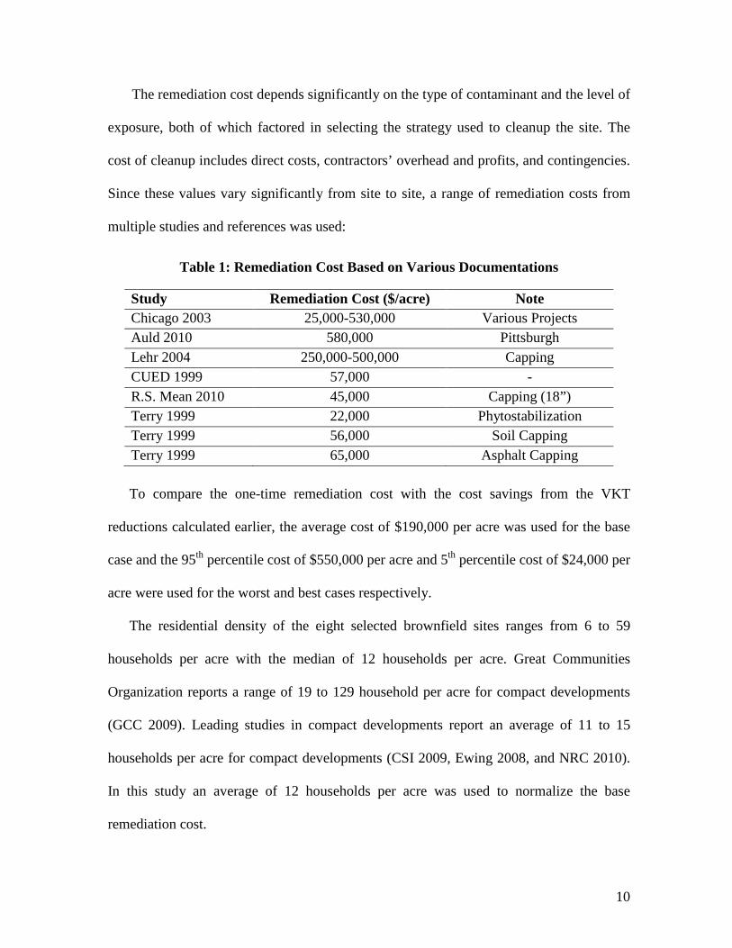
The remediation cost depends significantly on the type of contaminant and the level of
exposure, both of which factored in selecting the strategy used to cleanup the site. The
cost of cleanup includes direct costs, contractors’ overhead and profits, and contingencies.
Since these values vary significantly from site to site, a range of remediation costs from
multiple studies and references was used:
Table 1: Remediation Cost Based on Various Documentations
Study Remediation Cost ($/acre) Note Chicago 2003 25,000-530,000 Various Projects Auld 2010 580,000 Pittsburgh Lehr 2004 250,000-500,000 Capping CUED 1999 57,000 - R.S. Mean 2010 45,000 Capping (18”) Terry 1999 22,000 Phytostabilization Terry 1999 56,000 Soil Capping Terry 1999 65,000 Asphalt Capping To compare the one-time remediation cost with the cost savings from the VKT
reductions calculated earlier, the average cost of $190,000 per acre was used for the base
case and the 95th percentile cost of $550,000 per acre and 5th percentile cost of $24,000 per
acre were used for the worst and best cases respectively.
The residential density of the eight selected brownfield sites ranges from 6 to 59
households per acre with the median of 12 households per acre. Great Communities
Organization reports a range of 19 to 129 household per acre for compact developments
(GCC 2009). Leading studies in compact developments report an average of 11 to 15
households per acre for compact developments (CSI 2009, Ewing 2008, and NRC 2010).
In this study an average of 12 households per acre was used to normalize the base
remediation cost.
11
3. Results
3.1 VKT Comparison Results for Brownfield and Greenfield Sites
VKTs were calculated for eight brownfield and eight greenfield sites within the four
selected cities of Baltimore, Chicago, Minneapolis and Pittsburgh. Table 2 compares
HBW automobile VKTs, trip distance and the number of trips per household for
brownfields and greenfields.
Table 2: Brownfield and Greenfield Developments’ Travel Pattern Comparisons – Daily Home Based Work (HBW) Auto Trips per Household
12 cities: Atlanta, Baltimore, Boston, Charlotte, Denver, Dallas, Nashville, Sacramento, San Diego, Montgomery, Wes Palm Beach, BCD
Brownfield 61% 39% - 81% -
US Conference of Mayors (USCM), 2001
Baltimore and Dallas Brownfield - 23% - 55% 36%-87%*
EPA 2006 Atlantic Station, Atlanta Brownfield 73%** 14%-52% - CSI 2009, U.S. Compact 40% 20%-60% 20%-60% NCR 2010 U.S. Compact - 5%-25% 5%-25% Ewing 2008, U.S. Compact 30% 20%-40% 18%-36%
Nagengast, 2010 Minneapolis, Baltimore, Chicago, St. Louis, Pittsburgh, Milwaukee,
Brownfield *** *** 36%
*Actual number reported is 73%. The range was from pre-development model. ** The range is only showing the reduction of VOC and NOx. *** Nagengast does not directly calculate VKT, but rather focuses on travel time for commuting only and concludes that travel time for brownfields is only 3 minutes less than greenfields for all modes. Modal shares differed between the brownfield and greenfield developments, with transit share higher for brownfields.
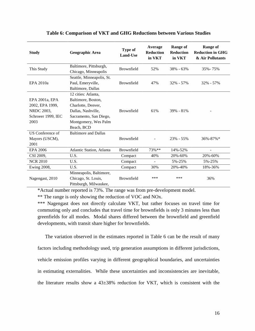
The variation observed in the estimates reported in Table 6 can be the result of many
factors including methodology used, trip generation assumptions in different jurisdictions,
vehicle emission profiles varying in different geographical boundaries, and uncertainties
in estimating externalities. While these uncertainties and inconsistencies are inevitable,
the literature results show a 43±38% reduction for VKT, which is consistent with the
17
results of this study (38%-63%). Furthermore, the literature results show a 46±41%
emissions reduction, which is consistent with the results of this study (35%-75%).
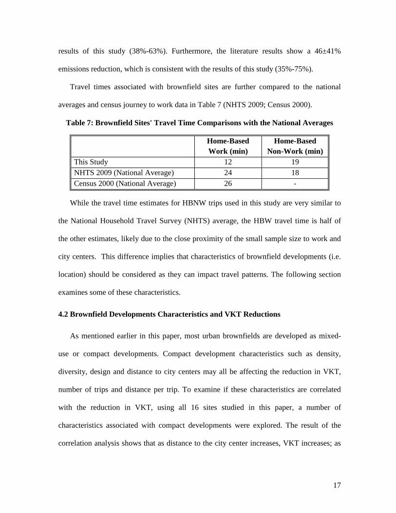
Travel times associated with brownfield sites are further compared to the national
averages and census journey to work data in Table 7 (NHTS 2009; Census 2000).
Table 7: Brownfield Sites' Travel Time Comparisons with the National Averages
Home-Based Work (min)
Home-Based Non-Work (min)
This Study 12 19 NHTS 2009 (National Average) 24 18 Census 2000 (National Average) 26 -
While the travel time estimates for HBNW trips used in this study are very similar to
the National Household Travel Survey (NHTS) average, the HBW travel time is half of
the other estimates, likely due to the close proximity of the small sample size to work and
city centers. This difference implies that characteristics of brownfield developments (i.e.
location) should be considered as they can impact travel patterns. The following section
examines some of these characteristics.
4.2 Brownfield Developments Characteristics and VKT Reductions
As mentioned earlier in this paper, most urban brownfields are developed as mixed-
use or compact developments. Compact development characteristics such as density,
diversity, design and distance to city centers may all be affecting the reduction in VKT,
number of trips and distance per trip. To examine if these characteristics are correlated
with the reduction in VKT, using all 16 sites studied in this paper, a number of
characteristics associated with compact developments were explored. The result of the
correlation analysis shows that as distance to the city center increases, VKT increases; as
18
access to transit improves, VKT decreases; and as walkability improves, VKT decreases.
Furthermore, brownfield developments show wider and higher range of density associated
with less VKT, while greenfield developments show less dense developments (less than 3
households/acre) with higher VKTs. A detailed discussion of the correlation analysis may
be found in the Appendix.
4.3 Brownfield Developments and Other Social and Economic Factors
Although time, fuel and environmental cost savings of brownfield developments are
important factors when it comes to making decisions to move to urban areas, vacancy
rates of the 16 study developments show the average vacancy rate of brownfield
developments is higher (9%) than greenfield developments (1%). So the question is if
moving to brownfield developments would save about 60% on the cost of fuel and time,
why is the vacancy rate higher in urban cores? Factors such as home value, property taxes,
crime rate and quality of schools are known to be among the most significant factors
influencing vacancy rates. Examining the average home values and property taxes, it was
concluded that for the 16 study sites examined in this paper, property tax and home values
are not the major determining factors. Other factors such as crime rate or quality of
schools may affect people’s decision more significantly. Details on vacancy rates, home
values and property taxes may be found in the Appendix.
6. Conclusions
In this paper, we have estimated and compared VKTs and their resulting costs of time,
fuel and emissions for eight brownfield and eight greenfield sites in Baltimore, Chicago,
Minneapolis and Pittsburgh, showing that residential brownfields generate significant
19
VKT reduction and cost savings. Brownfield developments on average result in about
$2,900 cost savings per household ($2,400/HH from time and fuel savings and $450 form
the external environmental cost savings). These estimates can be used in benefit-cost
studies to assess the benefits of travel reduction through land use changes and specifically
brownfield developments.
Acknowledgements
This material is based upon work supported by the National Science Foundation (Grant
No. 0755672) and the U.S. Environmental Protection Agency (Brownfield Training
Research and Technical Assistance Grant). Any opinions, findings, and conclusions or
recommendations expressed in this material are those of the author and do not necessarily
reflect the views of the Environmental Protection Agency or the National Science
Foundation.
20
References [AASHTO 2008] The American Association of State Highway and Transportation Officials. (2008). Primer on Transportation and Climate Change. [Retrieved from http://downloads.transportation.org/ClimateChange.pdf]. [Auld 2010] Auld, R., Hendrickson, C., and Lange, D. (2010).. A Life Cycle Assessment Case Study of a Brownfield and a Greenfield Development: Cranberry Heights and Summerset Pennsylvania. Carnegie Mellon University. Business of Brownfields Conferences Proceeding. [Census 2009] United States Census Bureau, 2000 Decennial Census,
http://factfinder.census.gov/home/saff/main.html?_lang=en (Accessed December 2010)
[Chester 2010] Chester, M. and Horvath, A. (2010), Comparison of Life-cycle Energy and Emissions Footprints of Passenger Transportation in Metropolitan Regions. Atmospheric Environment, 44(8), pp. 1071-1079, DOI:10.1016/j.atmosenv.2009.12.012. [Chicago. 2003] Chicago Brownfields Initiative Recycling Our Past, Investing in Our Future. (2003). [Retrieved from http://www.csu.edu/cerc/ documents/ ChicagoBrownfieldsInitiative RecyclingOurPastInvestinginOurFuture.pdf] [CSI 2009] Cambridge Systematics, Inc. (2009). Moving Cooler: An Analysis of Transportation Strategies for Reducing Greenhouse Gas Emissions. Washington, D.C.: Urban Land Institute. [CNT 2004] Center for Neighborhood Technology. (2004). Making the Case For Mixed Income and Mixed Use Communities : Solutions to the Emerging Affordability Crisis. [Retrieved from http://www.cnt.org/repository/MICI-Exec-Summary.pdf]. [CUED 1999] The Council of Urban Economic Development. (1999). Brownfields Redevelopment: Performance Evaluation. Washington DC [De Sousa 2005] De Sousa, C. (2005). Policy Performance and Brownfield Redevelopment in Milwaukee, Wisconsin. The Professional Geographer, 57(2), pp. 312-327.
[DNR 2006] Missouri Department of Natural Resources. (2006). Hidden Treasures:Value in Brownfields. [Dockins 2004] Dockins, C., Maguire, K., Simon, N., Sullivan, M., Value of
Statistical Life Analysis and Environmental Policy: A White Paper. EPA 2004. [Retrieved from http://yosemite.epa.gov/ee/epa/eerm.nsf/vwAN/EE-0483-01.pdf/$file/EE-0483-01.pdf
[DOE/EIA 2008] U.S. Department of Energy/Energy Information Agency. (2008). Annual Energy Outlook Report # DOE/EIA-0383. [Retrieved from http://www.eia.doe.gov/oiaf/aeo/pdf/0383%282010%29.pdf]. [DOT 2010] Department of Transportation. (2010). Transportation’s role in reducing US. Greenhouse Gas Emissions Volume I Synthesis Report.to Congress. [Reterived from http://ntl.bts.gov/lib/32000/32700/32779/ DOT_Climate_Change_Report_-_April_2010_- _Volume_1_and_2.pdf]. [EPA 1999] Hagler Bailly Services, Inc. and Criterion Planners/Engineers. (1999). The Transportation and Environmental Impacts of Infill Versus Greenfield Development:A Comparative Case Study Analysis. U.S. Department of Energy [EPA 2001a] Environmental Protection Agency. (2001). Comparing Methodologies to Assess Transportation and Air Quality Impacts of Brownfield’s and Infill Development, Development, Community, and Environment Division, [EPA 231-R-01-001, August 2001]. [EPA 2001] Environmental Protection Agency. (2001) IEC and Cambridge Systematics, Inc. EPA Remediation Technology Cost Compendium Year 2000. [EPA 2002] Environmental Protection Agency. (2002). Quantifying Emissions Impacts of Brownfields and Infill Development. [EPA 2003] Environmental Protection Agency. (2003). MOBILE6 Vehicle Emission. Modeling Software. [Retrieved from http://www.epa.gov/otaq/m6.htm.] [EPA 2006] Environmental Protection Agency. (2006). Solving Environmental Problems through Collaboration: the Atlantic Steel Case Study. [EPA. 2009] Environmental Protection Agency. (2009). Brownfields and Land
22
Revitalization. [Retrieved from http://epa.gov/brownfields/]. [EPA 2010a] Environmental Protection Agency. (2010). Air and Water Quality Impacts of Brownfields Redevelopment (Draft). [Ewing 2008] Ewing, R. Bartholomew, K., Winkelman, S., Walters, J., and Chen, D. (2008). Growing Cooler: The Evidence on Urban Development and Climate Change, Washington, DC: Urban Land Institute. [FHWA 2008] Federal Highway Administration. (2008). Highway Statistics. [Retrieved from http://www.fhwa.dot.gov/policy/ohpi/hss/index.htm]. [GCC 2009] Great Communities Collaborative. (2009). The Benefits of Compact Development.[Retrieved from
http://greatcommunities.org/intranet/library/sites-tools/great- communities-toolkit/density.pdf]. [Gordon 1997] Gordon, P., and Richardson, H. (1997). Are Compact Cities a Desirable Planning Goal? Journal of the American Planning Association, 63(1), pp. 95-106. DOI: 10.1080/01944369708975727. [GREET 2008] The Greenhouse Gas, Regulated Emissions, and Energy Use in
Transportation (GREET) Model. U.S. Department of Energy, Argonne National Laboratory. [Retrieved from http://www.transportation.anl.gov/modeling_simulation/GREE].
[GWU 2001] The George Washington University. (2001). Public Policies and Private Decisions Affecting the Redevelopment of Brownfields: An Analysis of Critical Factors, Relative Weights and Areal Differentials. [Retrieved from http://www.gwu.edu/~eem/Brownfields/]. [Handy 2005] Handy, S., Cao, X., and Mokhtarian, P. (2005). Correlation or causality between the built environment and travel behavior? Evidence from Northern California. Transportation Research Part D: Transport and Environmen.10(6), pp. 427-444. DOI: 10.1016/j.trd.2005.05.002. [Harvey 2001] Miller, Harvey J. & Shih-Lung Shaw. (2001) Geographic
Information Systems for Transportation, Oxford University Press US. p. 248. ISBN 0-19-512394-8
[Hoehner 2005] Hoehner, C.M., Brennan Ramirez, L.K., Elliott, M.B., Handy, S.L., and Brownson, R.C. (2005).Perceived and objective environmental
23
measures and physical activity among urban adults.American journal of preventive medicine. 28(2), pp. 105-116. DOI: 10.1016/j.amepre.2004.10.023 [HUD 2010] US Department of Housing and Urban Development. (2010).HUD Aggregated USPS Administrative Data On Address Vacancies. [Retrieved from http://www.huduser.org/portal/datasets/usps.html] [IEC 2003] Industrial Economics, Inc. (2003). Analysis of Environmental and Infrastructure Costs Associated with Development in the Berkeley Charleston Dorchester Region, April 2003. (BCD, SC area). [Johnston 2006] Johnston, R., (2006). Review of U.S. and European Regional
Modeling Studies of Policies Intended to Reduce Motorized Travel, Fuel Use, and Emissions. Department Environmental Science and Policy. University of California - Davis. Victoria Transport Policy Institute. Victoria, BC.
[Kaufman 2006] Kaufman, D., and Cloutier, N. (2006). The Impact of Small Brownfields and Greenspaces on Residential Property Values. Journal of Real Estate Finance and Economics, 33, pp. 19-30. [Lange 2004] Lange, D., and McNeil, S. (2004). Clean It and They Will Come? Defining Successful Brownfield Development. Journal of Urban Planning and Development, 130(2), pp. 101. DOI: 10.1061/(ASCE)0733-9488(2004)130:2(101). [Lehr 2004] Lehr, J.H., (1997). Wiley's Remediation Technologies Handbook. Chicago, IL: The Heartland Institute. [Mashayekh 2010] Mashayekh, Y., Chester, M., Hendrickson C.T., Weber, C.L.
(2010). External Environmental Costs of Congestion in the U.S. Metropolitan Areas. Transportation Research, In Review.
[Matthews 2000] Matthews, H.S., and Lave, L.B., (2000). Applications of Environmental Valuation for Determining Externality Costs. Environmental Science and Technology, 34, pp. 1390-1395. DOI:10.1021/es9907313. [Muller 2007] Muller, N.Z., Mendelsohn, R., (2007). Measuring the Damages from Air Pollution in the U.S. Journal of Environmental Economics and Management, 54, pp. 1-14. [Nagengast 2010] Nagengast, A. (2010). Commuting from US Brownfield and Greenfield Residential Development Neighborhoods. ASCE, 1-32.
24
[Reterived from http://www.eswp.com/brownfields/Present/Nagengast%205B.pdf] [NHTS 2009] National Household Travel Survey.[2009] [Retrieved from http://nhts.ornl.gov/]. [NRC 2009] The National Research Council of the National Academies. (2009). Driving and the Built Environment: The Effects of Compact Development on Motorized Travel, Energy Use, and CO2 Emissions. Transportation Research, Special Report 298. [NRC 2010] The National Research Council of the National Academies. (2010). Committee on Health, Environmental, and Other External Costs and Benefits of Energy Production and Consumption; National Research Council, Hidden Cost of Energy: Unpriced Consequences of Energy Production and Use, National Academies Press. [NRDC 2003] Allen, E., Benfield, F.K., (2003). Environmental Characteristics of Smart Growth Neighborhoods, Phase II: Two Nashville Neighborhoods. Natural Resources Defense Council. [Retrieved from http://www.nrdc.org/cities/smartgrowth/char/charnash.pdf] [OTA 1995] U.S. Congress, Office of Technology Assessment. (1995). The Technological Reshaping of Metropolitan America, OTA-ETI- 643 Washington, DC: U.S. Government Printing Office. [O’Toole 2009] O’Toole, R. The Myth of the Compact City Why Compact Development Is Not the Way to Reduce Carbon Dioxide Emissions. Policy Analysis 653. [Retrieved from http://www.cato.org/pubs/pas/pa653.pdf [Paull 2008] Paul E. (2008). The Environmental and Economic Impacts of Brownfields Redevelopment. Northeast-Midwest Institute. [Retrieved from http://www.nemw.org/images/stories/documents/ EnvironEconImpactsBFRedev.pdf] [Rast 1997] Rast, R.R. (1997). Environmental Remediation Estimating Methods. Kingston, MA:R.S.Means. [Ross 1994] Ross M. Automobile Fuel Consumption and Emissions: Effects of Vehicle and Driving Characteristics, Annual Review of Energy and the Environment, 19. pp.75-112, [RS Means 2010] RS Means Cost Estimation Tools.(2010). [Retrieved from http://rsmeans.reedconstructiondata.com/MeansCostWorks.aspx].
25
[Schroeer 1999] Schroeer, W., (1999). Transportation and Environmental Analysis of the Atlantic Steel Development Proposal. Prepared for U. S. Environmental Protection Agency, Urban and Economic Development Division. [Shammin 2010] Shammin, M. R., Herendeen, R. a, Hanson, M. J., and Wilson, E. J. H. (2010). A Multivariate Analysis Of The Energy Intensity of Sprawl Versus Compact Living in The U.S. For 2003. Ecological Economics, 69(12), 2363-2373. Elsevier B.V. DOI: 10.1016/j.ecolecon.2010.07.003. [Terry 1999] Terry, N., and Banuelos, G. (1999). Phytoremediation of Contaminated Soil and Water. Boca Raton,FL:Lewis Publication. [TF 2009] Tax Foundation. (2009). Tax Foundation website.
[http://www.Taxfoundation.org] [TTI 2009] Texas Transportation Institute, Lomax, T. (2009). Urban Mobility
Report.Texas Transportation Institute. [USCM 2001] The US Conference of Mayors, Clean Air/Brownfields Report. Environmental Protection. (2001). [Retrieved from http://usmayors.org/brownfields/CleanAirBrownfields02.pdf]. [US FSTP 2009] S. 1036: Federal Surface Transportation Policy and Planning Act of 2009. [Retrieved from http://www.govtrack.us/congress/bill.xpd?bill=s111-1036]. [US GAO 2004] The government Accountability Office. (2004). Brownfield Redevelopment. Stakeholders Report That EPA’s Program Helps to Redevelop Sites, but Additional Measures Could Complement Agency Efforts. [Retrieved from http://www.gao.gov/new.items/d0594.pdf]. [Wang 2007] Wange, X., and Hofe, Rainer Vom, (2007). Research Methods in
Urban and Regional Planning. Tsinghua University Press, Beijing and Springer. ISBN 978-3-540-49657-1.
26
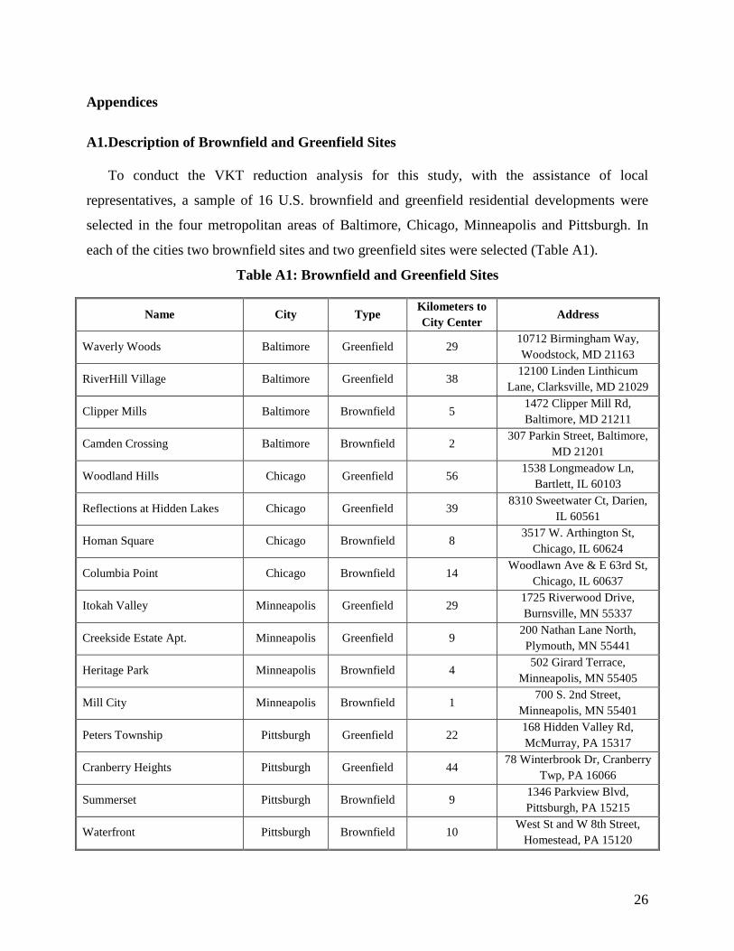
Appendices
A1. Description of Brownfield and Greenfield Sites
To conduct the VKT reduction analysis for this study, with the assistance of local
representatives, a sample of 16 U.S. brownfield and greenfield residential developments were
selected in the four metropolitan areas of Baltimore, Chicago, Minneapolis and Pittsburgh. In
each of the cities two brownfield sites and two greenfield sites were selected (Table A1).
showes as transit time increases, HBW trips also increase (not as strong for HBNW trips, ρHBNW
= 0.5), and walkability showing as the power of walkability increases, VKT deacreases (ρHBW = -
0.64, ρHBNW = - 0.4) were also examined. Compared with other factors, density shows a weak
correlation with HBW trips (ρHBW = -0.5) and almost no correlation with HBNW trips (ρHBW = -
0.02). Figure A1 shows that, in general, greenfield developments have lower density (typically
below 3 households per acre) and higher VKTs while brownfield developments have higher
densities with wider range and fewer VKTs.
31
Figure A7: Home Based Work (HBW) Daily VKT vs. Density
A7. Vacancy Rates, Home Values and Property Taxes
Economic and social factors such as home value, property taxes, crime rate, and quality of
schools influence people’s decisions when it comes to moving to urban cores to live in
brownfield developments. Although the focus of this paper is not on the social aspects of
brownfield developments, vacancy rates of the 16 study developments were studied to examine
what factors might influence people’s decisions. The question was if households would save
60% on the cost of time and fuel by moving to brownfield developments, what is stopping them?
Vacancy rates, calculated from the 2010 United States Postal Services data on houses that
have been vacant in the past 90 days (HUD, 2010). For brownfield developments, the average
vacancy rates is about 9% while for greenfield developments the rate is about 1%. The
difference is statistically significant with 95% confidence (p=0.002). To examine if the home
value or the property tax is affecting vacancy rates, the 2009 median home values and property
taxes were examined. The average home value of the brownfield developments is about
32
$220,000 while the average home value of the greenfield developments is about $290,000 (TF,
2009). Home values might be simply higher in or around greenfield developments as properties
generally have more land resulting in a higher price. The 2009 property tax data for the sixteen
sites shows that the average property tax of brownfield developments is 1.4% while the average
property tax of greenfield developments is about 1.3% (TF 2009). While we recognize that the
sample size is small, we conclude that, for the study sites, property tax and home values are not
the major determining factors in making housing decisions. Other factors such as rate of crime or
quality of schools may be affecting people’s decision more significantly.
33
APPENDIX B
PAPER PRESENTED IN JANUARY 2011 AT THE 90TH ANNUAL TRANSPORTATION
RESEARCH BOARD CONFERENCE IN WASHINGTON D.C. THE PAPER HAS BEEN
ACCEPTED TO BE PUBLISHED IN TRANSPORTATION RESEARCH RECORDS
(TRR) DURING THE SPRING OF 2011.
Title: Costs of Automobile Air Emissions in U.S. Metropolitan Areas Yeganeh Mashayekh (Corresponding Author) Ph.D. Student Department of Civil & Environmental Engineering Department of Engineering & Public Policy Carnegie Mellon University, Pittsburgh, PA 15213-3890 Phone: 412-268-2940 [email protected] Paulina Jaramillo Assistant Research Professor Department of Engineering and Public Policy Carnegie Mellon University, Pittsburgh, PA 15213-3890 Phone: 412-268-7889 [email protected] Mikhail Chester Post-doctoral Researcher Department of Civil & Environmental Engineering 407 McLaughlin Hall, University of California, Berkeley, CA 94720 Phone: 510-761-6414 [email protected] Chris T. Hendrickson Duquesne Light Professor of Engineering Department of Civil and Environmental Engineering Carnegie Mellon University, Pittsburgh, PA 15213-3890 Phone: 412-268-2940 [email protected] Christopher L. Weber Research Assistant Professor Department of Civil & Environmental Engineering Carnegie Mellon University, Pittsburgh, PA 15213-3890 Phone: 412-268-2940 [email protected] Number of words (including tables and figures): 7,300 Number of figures: 4 Number of tables: 5
forest recreation) damages. APEEP factors for a value of statistical life of $6M are used for this
paper. Population weighted average APEEP factors are determined for each urban region
analyzed in this study.
The cost of CO, since not provided by APEEP, was assumed to be $0.7/kg (Matthews 2001).
This value was regionally scaled for each urban area analyzed using the ratios for NOx observed
in the APEEP data, since both pollutants are predominantly tropospheric ozone precursors. CO2
40
costs are based on a literature survey performed by NRC 2010. A summary of CO2-eq units costs
from roughly 50 studies shows a median cost of $10/ton, mean cost of $30/ton, and 5th and 95th
percentile costs of $1 and $85/ton [NRC 2010]. The mean $30/ton cost is implemented for
vehicle CO2 emissions here.
Vehicle emission factors were increased by 4.9% annually for CO, 1.4% for NOX, 4.5% for
PM2.5 and 5.9% for VOCs to capture the effects of fleet age and improving emissions trends due
to more stringent emissions standards and improved fuel programs (Chester 2010). The average
vehicle age is assumed to be 5 years (GREET 2008).
The above calculated emission factors and costs were then applied to the 2007 TTI mobility
data (TTI 2009) for 86 urban areas. As previously discussed, four urban areas in TTI (2009) were
discarded due to lack of valuation data in the APEEP model. Volume and speed (congestion and
free flow) data utilized in the TTI report were all collected from freeway operation centers in
various urban areas. TTI provides the percentage of miles travelled in each urban area during
peak times and non-peak times. For non-peak miles, free flow speeds of 60 and 35 miles per
hour (mph) for freeways and arterials, respectively, were used in this analysis. For peak times,
TTI provides the percentage of travel that is congested and an average congested speed. Rather
than unrealistically assuming constant speed under congested conditions, it was assumed that
some percentage of vehicles operating during congested peak times drove at a stop and go speed
of 5 mph and the remaining vehicles drove close to free flow speeds (free flow speed less one
mile per hour). The percentages were estimated so that the weighted average speed matched the
congested speed given by TTI. For non-congested peak travel, free flow speeds prevailed.
4. Results for External Air Emissions Costs
The total external air emissions costs of light duty vehicle travel for the 86 urban areas used
in this analysis is estimated to be $145 million per day in 2007 U.S. dollars. This averages to
around 1.7 million dollars per day per urban area. Normalizing the results by population and
VMT, the external cost of driving is $0.64 per person per day or $0.03 per VMT. These
estimates are higher than the national average of 1.3 cents/VMT in NRC (2010) because we are
only considering urban areas and we are including a cost for carbon dioxide emissions. Table 1
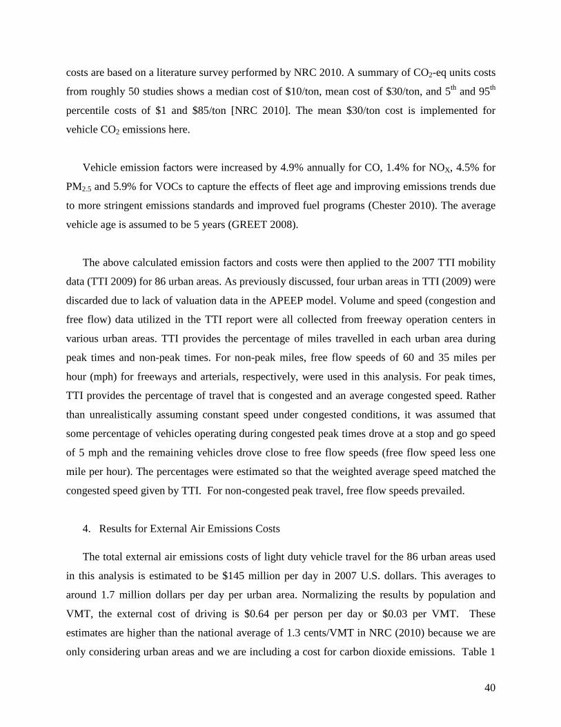
41
shows a subset of the urban areas with the top 10 external costs (due to a combination of large
populations and high external cost factors). The complete list of the external air emissions costs
is available from the authors.
Table 8: External Air Emission Costs, population, per capita vehicle miles traveled, and percentage of peak travel that is congested of Driving for Top 10 Urban Areas
Urban Area Million $/Day
$/Day/Person $/VMT Population VMT/
person % Peak travel
congested Los Angeles-Long Beach-Santa Ana CA 23 1.8 0.086 12,800,000 21 86 New York-Newark NY-NJ-CT 23 1.3 0.10 18,225,000 12 69 Chicago IL-IN 10 1.2 0.10 8,440,000 12 79 Philadelphia PA-NJ-DE-MD 4.9 0.9 0.058 5,310,000 16 63 Washington DC-VA-MD 4.6 1.1 0.057 4,330,000 19 81 San Francisco-Oakland CA 4.5 1.0 0.056 4,480,000 18 82 Atlanta GA 4.3 1.0 0.046 4,440,000 21 75 Dallas-Fort Worth-Arlington TX 4.2 0.95 0.042 4,445,000 23 66 Detroit MI 3.9 1.0 0.045 4,050,000 21 71 Houston TX 3.9 1.0 0.043 3,815,000 24 73
Total* 145 158,355,000
Average* 1.7 0.64 0.034 1,841,000 19 48
Maximum* 23.0 1.8 0.10 18,225,000 30 86
Minimum* 0.038 0.18 0.013 145,000 10 8.0 *Average, total, maximum and minimum values are for all 86 urban areas.
Los Angeles and New York have the largest population among the 86 urban areas and their
total external emissions cost, each around $23 million/day, are roughly twice as large as the next
largest cost area (Chicago, $10 million/day). After Chicago, another halving occurs to
Philadelphia, Washington DC, San Francisco, and so on. The largest driver for having large
external costs is clearly population, as 8 of the top 10 most populous metropolitan statistical
areas (MSAs) are represented in the top external cost list—only Miami and Boston MSAs are not
and they represent the 12th and 13th rank on external costs. Looking at the normalized data shows
a wide variation between the top 3 areas—Los Angeles, New York, and Chicago—and the
others, though some other areas have high per capita (Washington DC) or per VMT
(Philadelphia) costs. The differences between normalized values are attributable to density and
the APEEP factors, which evaluate pollutant transport, chemistry, and impact on nearby
populations (Muller 2007).
42
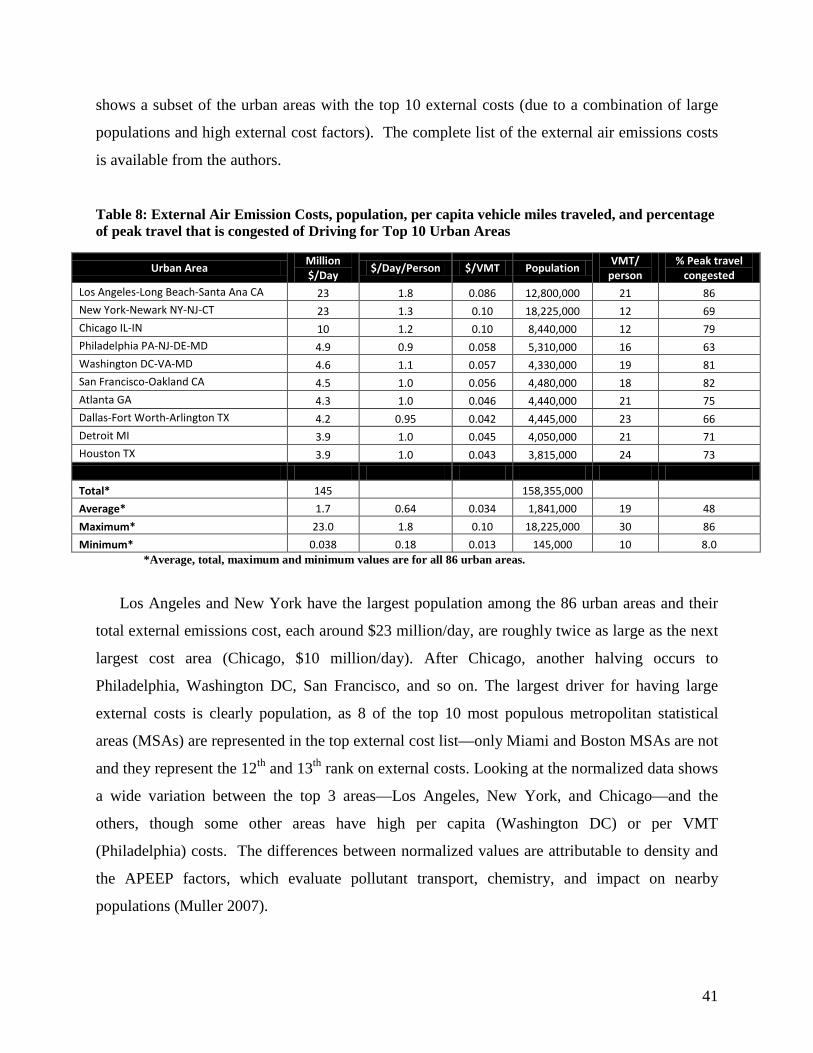
Table 2 shows the $145 million total external emissions cost of driving and congestion
disaggregated by pollutant for all 86 urban areas. Carbon dioxide emissions valued at $ 30/mt
are comparable in external costs to VOCs, CO and NH3 costs, while three other pollutants
(nitrogen oxides, sulfur dioxide and particulates) have lower magnitudes.
Table 9: External Emissions Cost of Driving per Pollutant (Million $/Day)
CO2 NOx VOCs CO SOx PM NH3 Total Cost of Driving 32 7.6 39 31 0.65 3.4 31
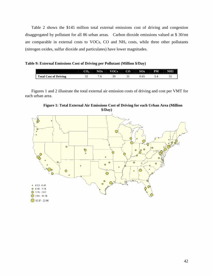
Figures 1 and 2 illustrate the total external air emission costs of driving and cost per VMT for
each urban area.
Figure 1: Total External Air Emissions Cost of Driving for each Urban Area (Million $/Day)
43
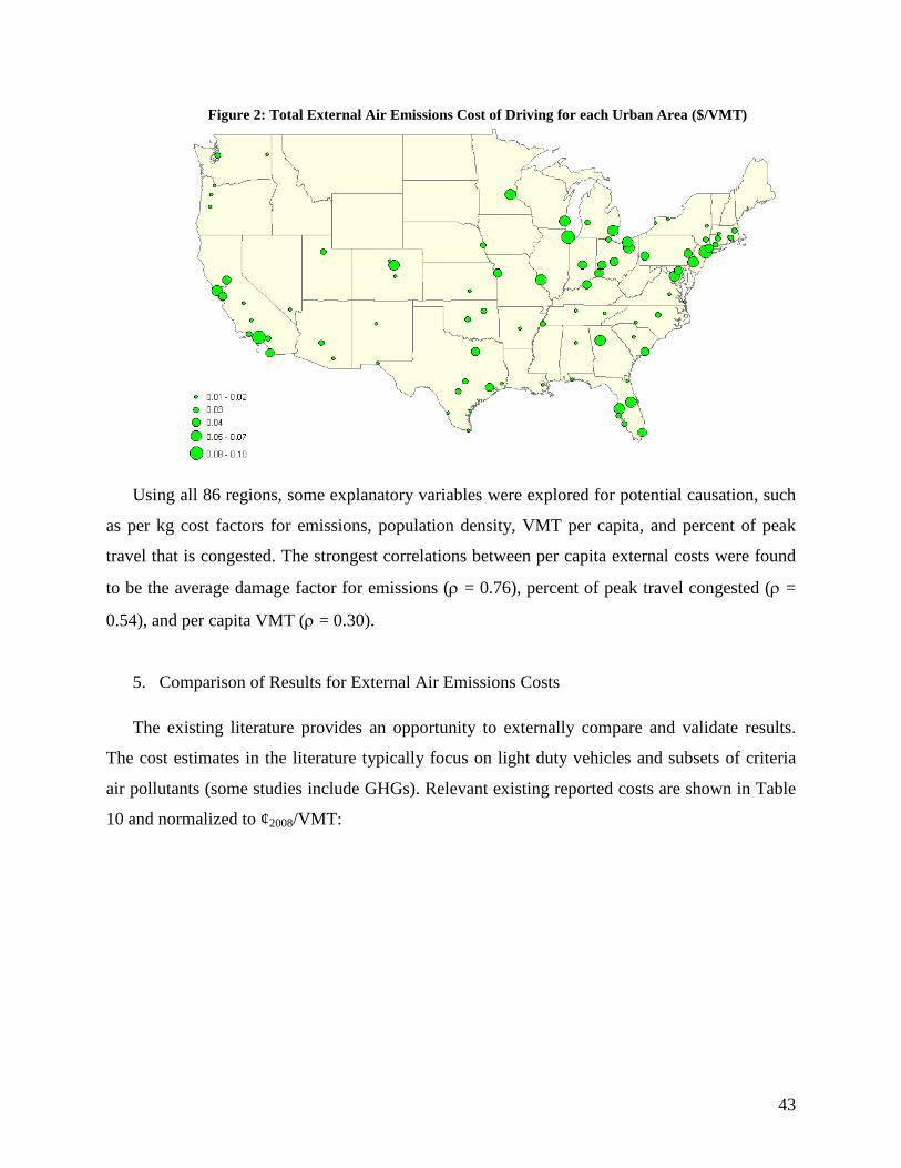
Figure 2: Total External Air Emissions Cost of Driving for each Urban Area ($/VMT)
Using all 86 regions, some explanatory variables were explored for potential causation, such
as per kg cost factors for emissions, population density, VMT per capita, and percent of peak
travel that is congested. The strongest correlations between per capita external costs were found
to be the average damage factor for emissions (ρ = 0.76), percent of peak travel congested (ρ =
0.54), and per capita VMT (ρ = 0.30).
5. Comparison of Results for External Air Emissions Costs
The existing literature provides an opportunity to externally compare and validate results.
The cost estimates in the literature typically focus on light duty vehicles and subsets of criteria
air pollutants (some studies include GHGs). Relevant existing reported costs are shown in Table
10 and normalized to ¢2008/VMT:
44
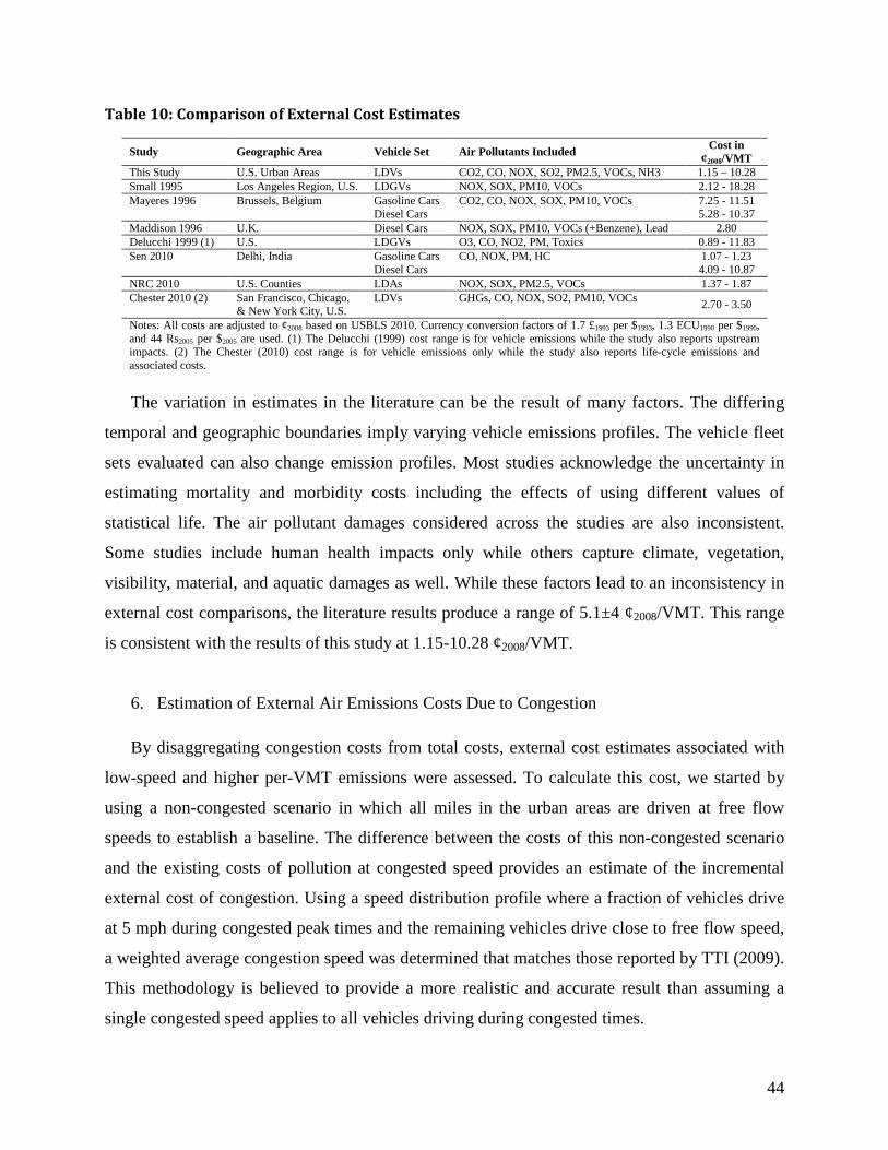
Table 10: Comparison of External Cost Estimates
Study Geographic Area Vehicle Set Air Pollutants Included Cost in ¢2008/VMT
This Study U.S. Urban Areas LDVs CO2, CO, NOX, SO2, PM2.5, VOCs, NH3 1.15 – 10.28 Small 1995 Los Angeles Region, U.S. LDGVs NOX, SOX, PM10, VOCs 2.12 - 18.28 Mayeres 1996 Brussels, Belgium Gasoline Cars CO2, CO, NOX, SOX, PM10, VOCs 7.25 - 11.51 Diesel Cars 5.28 - 10.37 Maddison 1996 U.K. Diesel Cars NOX, SOX, PM10, VOCs (+Benzene), Lead 2.80 Delucchi 1999 (1) U.S. LDGVs O3, CO, NO2, PM, Toxics 0.89 - 11.83 Sen 2010 Delhi, India Gasoline Cars CO, NOX, PM, HC 1.07 - 1.23 Diesel Cars 4.09 - 10.87 NRC 2010 U.S. Counties LDAs NOX, SOX, PM2.5, VOCs 1.37 - 1.87 Chester 2010 (2) San Francisco, Chicago,
& New York City, U.S. LDVs GHGs, CO, NOX, SO2, PM10, VOCs 2.70 - 3.50
Notes: All costs are adjusted to ¢2008 based on USBLS 2010. Currency conversion factors of 1.7 £1993 per $1993, 1.3 ECU1990 per $1990, and 44 Rs2005 per $2005 are used. (1) The Delucchi (1999) cost range is for vehicle emissions while the study also reports upstream impacts. (2) The Chester (2010) cost range is for vehicle emissions only while the study also reports life-cycle emissions and associated costs.
The variation in estimates in the literature can be the result of many factors. The differing
temporal and geographic boundaries imply varying vehicle emissions profiles. The vehicle fleet
sets evaluated can also change emission profiles. Most studies acknowledge the uncertainty in
estimating mortality and morbidity costs including the effects of using different values of
statistical life. The air pollutant damages considered across the studies are also inconsistent.
Some studies include human health impacts only while others capture climate, vegetation,
visibility, material, and aquatic damages as well. While these factors lead to an inconsistency in
external cost comparisons, the literature results produce a range of 5.1±4 ¢2008/VMT. This range
is consistent with the results of this study at 1.15-10.28 ¢2008/VMT.
6. Estimation of External Air Emissions Costs Due to Congestion
By disaggregating congestion costs from total costs, external cost estimates associated with
low-speed and higher per-VMT emissions were assessed. To calculate this cost, we started by
using a non-congested scenario in which all miles in the urban areas are driven at free flow
speeds to establish a baseline. The difference between the costs of this non-congested scenario
and the existing costs of pollution at congested speed provides an estimate of the incremental
external cost of congestion. Using a speed distribution profile where a fraction of vehicles drive
at 5 mph during congested peak times and the remaining vehicles drive close to free flow speed,
a weighted average congestion speed was determined that matches those reported by TTI (2009).
This methodology is believed to provide a more realistic and accurate result than assuming a
single congested speed applies to all vehicles driving during congested times.
45
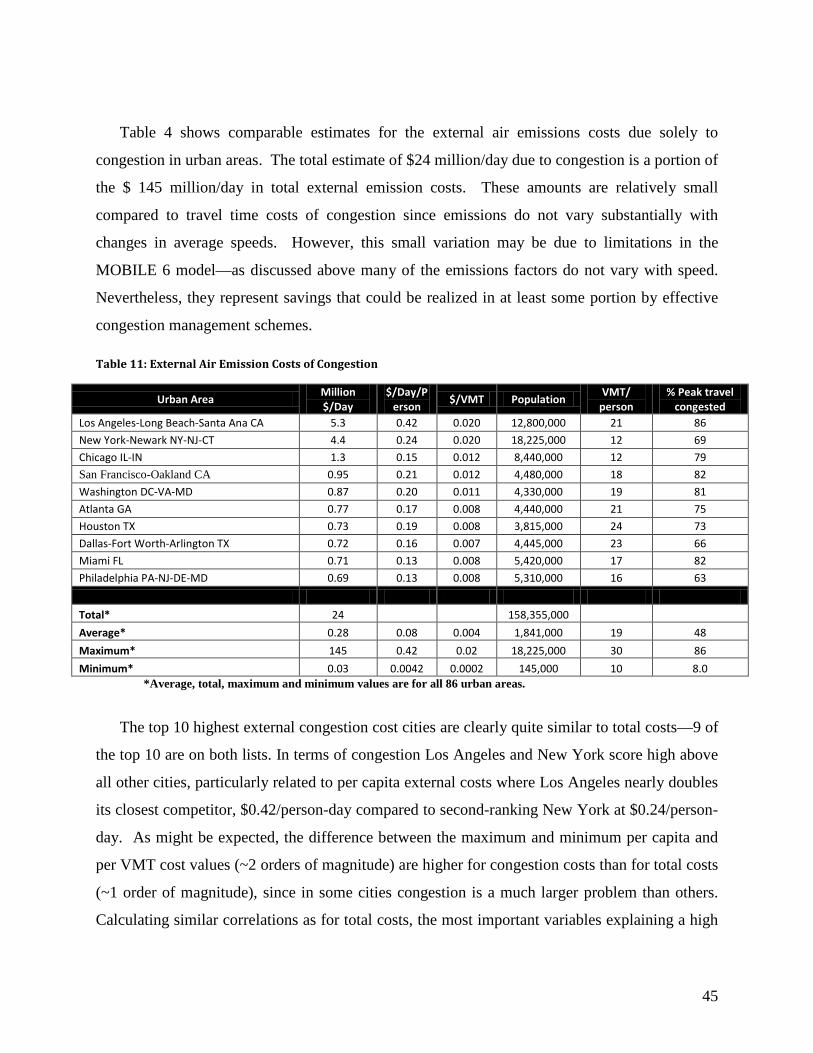
Table 4 shows comparable estimates for the external air emissions costs due solely to
congestion in urban areas. The total estimate of $24 million/day due to congestion is a portion of
the $ 145 million/day in total external emission costs. These amounts are relatively small
compared to travel time costs of congestion since emissions do not vary substantially with
changes in average speeds. However, this small variation may be due to limitations in the
MOBILE 6 model—as discussed above many of the emissions factors do not vary with speed.
Nevertheless, they represent savings that could be realized in at least some portion by effective
congestion management schemes.
Table 11: External Air Emission Costs of Congestion
Urban Area Million $/Day
$/Day/Person
$/VMT Population VMT/
person % Peak travel
congested Los Angeles-Long Beach-Santa Ana CA 5.3 0.42 0.020 12,800,000 21 86
New York-Newark NY-NJ-CT 4.4 0.24 0.020 18,225,000 12 69
Chicago IL-IN 1.3 0.15 0.012 8,440,000 12 79
San Francisco-Oakland CA 0.95 0.21 0.012 4,480,000 18 82
Washington DC-VA-MD 0.87 0.20 0.011 4,330,000 19 81
Philadelphia PA-NJ-DE-MD 0.69 0.13 0.008 5,310,000 16 63
Total* 24 158,355,000
Average* 0.28 0.08 0.004 1,841,000 19 48
Maximum* 145 0.42 0.02 18,225,000 30 86
Minimum* 0.03 0.0042 0.0002 145,000 10 8.0 *Average, total, maximum and minimum values are for all 86 urban areas.
The top 10 highest external congestion cost cities are clearly quite similar to total costs—9 of
the top 10 are on both lists. In terms of congestion Los Angeles and New York score high above
all other cities, particularly related to per capita external costs where Los Angeles nearly doubles
its closest competitor, $0.42/person-day compared to second-ranking New York at $0.24/person-
day. As might be expected, the difference between the maximum and minimum per capita and
per VMT cost values (~2 orders of magnitude) are higher for congestion costs than for total costs
(~1 order of magnitude), since in some cities congestion is a much larger problem than others.
Calculating similar correlations as for total costs, the most important variables explaining a high
46
congestion cost were percent of peak travel congested (ρ = 0.84), pollution cost (ρ = 0.76), and
population density (ρ = 0.52).
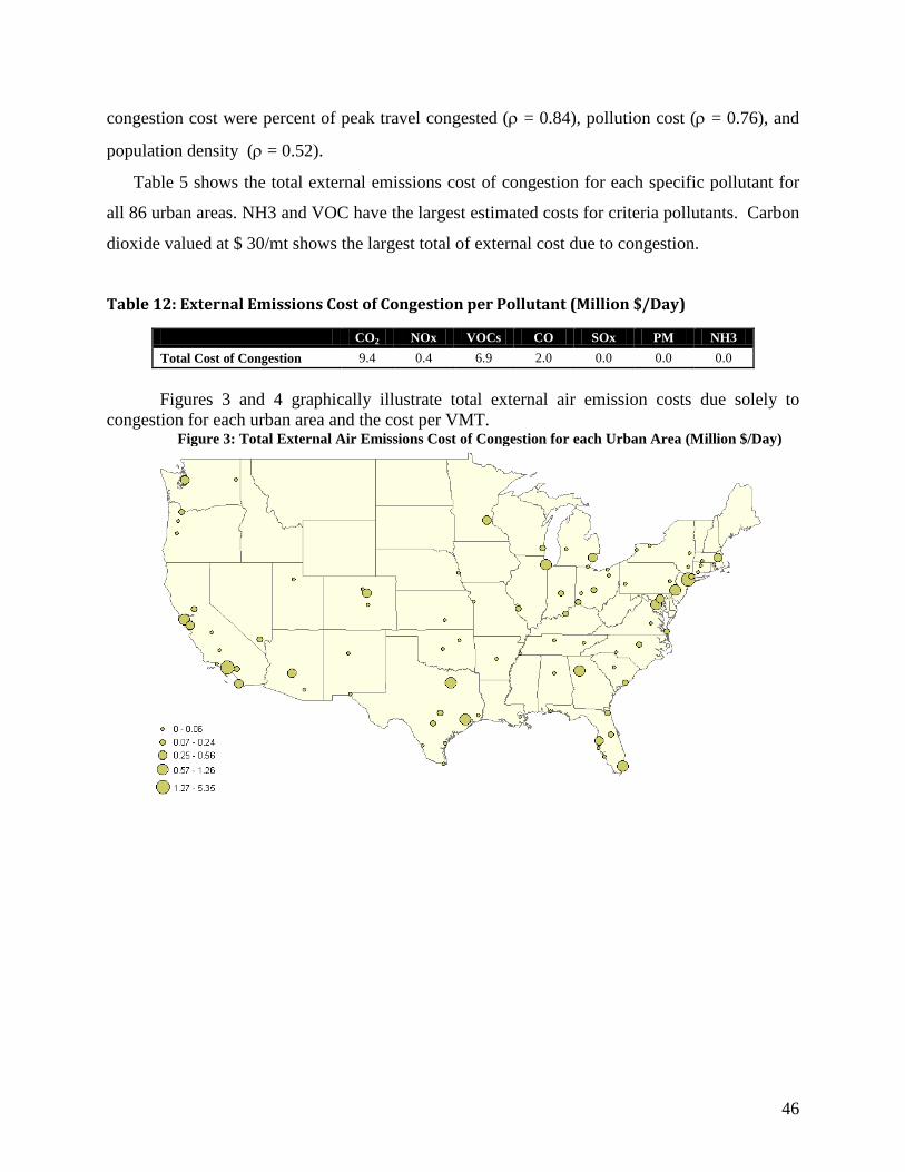
Table 5 shows the total external emissions cost of congestion for each specific pollutant for
all 86 urban areas. NH3 and VOC have the largest estimated costs for criteria pollutants. Carbon
dioxide valued at $ 30/mt shows the largest total of external cost due to congestion.
Table 12: External Emissions Cost of Congestion per Pollutant (Million $/Day)
CO2 NOx VOCs CO SOx PM NH3 Total Cost of Congestion 9.4 0.4 6.9 2.0 0.0 0.0 0.0
Figures 3 and 4 graphically illustrate total external air emission costs due solely to
congestion for each urban area and the cost per VMT. Figure 3: Total External Air Emissions Cost of Congestion for each Urban Area (Million $/Day)
47
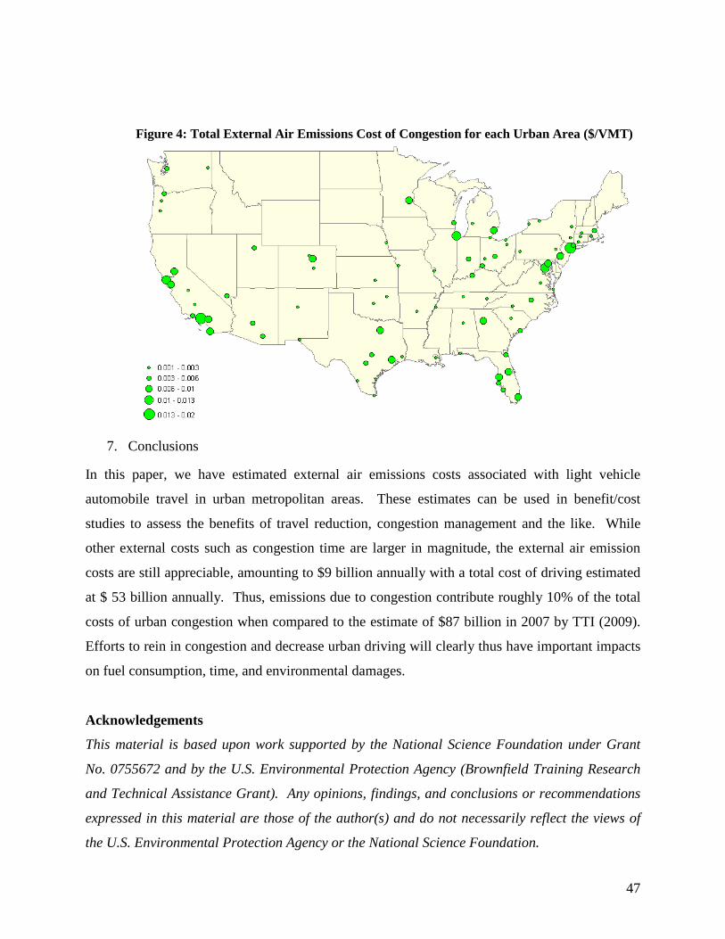
Figure 4: Total External Air Emissions Cost of Congestion for each Urban Area ($/VMT)
7. Conclusions
In this paper, we have estimated external air emissions costs associated with light vehicle
automobile travel in urban metropolitan areas. These estimates can be used in benefit/cost
studies to assess the benefits of travel reduction, congestion management and the like. While
other external costs such as congestion time are larger in magnitude, the external air emission
costs are still appreciable, amounting to $9 billion annually with a total cost of driving estimated
at $ 53 billion annually. Thus, emissions due to congestion contribute roughly 10% of the total
costs of urban congestion when compared to the estimate of $87 billion in 2007 by TTI (2009).
Efforts to rein in congestion and decrease urban driving will clearly thus have important impacts
on fuel consumption, time, and environmental damages.
Acknowledgements
This material is based upon work supported by the National Science Foundation under Grant
No. 0755672 and by the U.S. Environmental Protection Agency (Brownfield Training Research
and Technical Assistance Grant). Any opinions, findings, and conclusions or recommendations
expressed in this material are those of the author(s) and do not necessarily reflect the views of
the U.S. Environmental Protection Agency or the National Science Foundation.
48
49
References [AAA 2007] AAA American Automobile Association, Calculates Driving Cost at 52.2
Cents Per Mile for 2007, Automotive Article, March 2007, Orlando, Florida, http://www.aaanewsroom.net/main/Default.asp?CategoryID=4&ArticleID=529, Last accessed May 2010.
[Altshuler 1979] Altshuler, Alan A., Womack, James P., Pucher, John P. The Urban
Transportation System: Politics and Policy Innovation Cambridge, The M.I.T. Press. 1979, First Edition. (ISBN: 0262010550)
[Chester 2010] Chester M, Horvath A, and Madanat S, 2010, Comparison of life-cycle
energy and emissions footprints of passenger transportation in metropolitan regions 44(8) 1071-1079 (available online at http://dx.doi.org/10.1016/j.atmosenv.2009.12.012).
[Delucchi 1999] McCubbin D R and Delucchi M A, 1999, The Health Costs of Motor-
Vehicle-Related Air Pollution, Journal of Transportation Economics and Policy, 33(3), 253-286 [available online at http://www.jstor.org/stable/20053815].
[Delucchi 1998] Delucchi Mark, 1998, Report #1 in the series: The Annualized Social Cost
of Motor-Vehicle Use in the United States, based on 1990-1991 Data, Institute of Transportation Studies, University of California, Davis, UCD-ITS-RR-96-3 (1) rev. 1,
[EPA 2003] U.S. Environmental Protection Agency, 2003, MOBILE6 Vehicle
Emission Modeling Software, http://www.epa.gov/otaq/m6.htm, Last accessed May 2010.
[EPA 2010a] U.S. Environmental Protection Agency, 1995, Air Trends 1995,
http://www.epa.gov/air/airtrends/aqtrnd95/report/o3co.html Last accessed May 2010.
[EPA 2010b] U.S. Environmental Protection Agency, 2010, Transportation and Climate: Regulations
and Standards http://www.epa.gov/otaq/climate/regulations.htm Last accessed May 2010. [EPA 2010c] INVENTORY OF U.S. GREENHOUSE GAS EMISSIONS AND SINKS:
1990-2008 (April 2010) U.S. EPA # 430-R-10-006, http://www.epa.gov/climatechange/emissions/usinventoryreport.html, Last accessed May 2010.
[Fairfield 2010] Fairfield, Hannah, 2010, ‘Driving shifts into reverse,’ New York Times,
http://www.nytimes.com/imagepages/2010/05/02/business/02metrics.html, Last accessed June 2010.
[FHWA 2008] Federal Highway Administration, ‘Highway Statstics 2008, http://www.fhwa.dot.gov/policyinformation/statistics/2008/, Last visited May 2010.
[Granell 2004] Granell, J., et al., 2004. Analysis of mobile 6.2's PM emission factor
estimating function. In: U.S. Environmental Protection Agency's 13th International Emission Inventory Conference. http://www.epa.gov/ttn/chief/conference/ei13/mobile/granell.pdf. Last accessed May 2010.
[GREET 2008] The Greenhouse Gas, Regulated Emissions, and Energy Use in
Transportation (GREET) Model. U.S. Department of Energy, Argonne National Laboratory. http://www.transportation.anl.gov/modeling_simulation/GREET, Last visited May 2010.
[Maddison 1996] Maddison D, Pearce D, Johansson O, Calthorp E, Litman T, and Verhoef
E, 1996, Blueprint 5: The True Costs of Road Transport, Earthscan Publications Limited, UK, ISBN 1-85383-268-5.
[Maibach, 2008] Maibach, M. et al., 2008, Handbook on Estimation of External Cost in the
Transport Sector: Produced within the study Internalisation Measures and Policies for All external Cost of Transport (IMPACT) Version 1.1, CE Delft, for the European Commission DG TREN, http://ec.europa.eu/transport/costs/handbook/doc/2008_01_15_handbook_external_cost_en.pdf, Last accessed May 2010.
[Matthews, 2001] Matthews, H.S., Hendrickson, C.H., Horvath, A., 2001. External costs of
air emissions from transportation. ASCE Journal of Infrastructure Systems 7, 13e17. doi:10.1061/(ASCE)1076-0342(2001)7:1(13).
[Matthews, 2001] Matthews, H.S., Lave, L.B., 2000. Applications of environmental
valuation for determining externality costs. Environmental Science and Technology 34, 1390e1395. doi:10.1021/es9907313.
[Mayeres 1996] Mayeres I, Ochelen S, and Proost S, 1996, The Marginal External Costs of
Urban Transport, Transportation Research D: Transport and Environment, 1(2), 111-130 [available online at http://dx.doi.org/10.1016/S1361-9209(96)00006-5].
[Moffet 1993] Moffet, J and Miller P, 1993, The Price of Mobility, Natural Resources
Defense Council, 1993. [Muller 2007] Muller, N.Z., R.O. Mendelsohn. 2007. Measuring the Damages from Air
Pollution in the U.S. Journal of Environmental Economics and Management. 54: 1-14.
[NRC 2010] Committee on Health, Environmental, and Other External Costs and
Benefits of Energy Production and Consumption; National Research Council, Hidden Cost of Energy: Unpriced Consequences of Energy Production and Use, National Academies Press. 2010.
[Parrish 2006] Parrish, D.D., 2006. Critical evaluation of U.S. on-road vehicle emission
[Ross 1994] Ross M, 1994, Automobile Fuel Consumption and Emissions: Effects of
Vehicle and Driving Characteristics, Annual Review of Energy and the Environment 19 75-112, http://dx.doi.org/10.1146/annurev.eg.19.110194.000451, Last accessed May 2010.
[Saito 2010] Saito, K., et. Al., 2010, Traffic Congestion and Accident Externality: A
Japan-U.S. Comparison, The B.E. Journal of Economic Analysis & Policy, 10, issue 1, number 14, http://econpapers.repec.org/RePEc:bpj:bejeap:v:10:y:2010:i:1:n:14
Last accessed May 2010. [Sen 2010] Sen A K, Tiwari G, and Upadhyay V, 2010, Estimating Marginal External
Costs of Transport in Delhi, Transport Policy, 17(1), 27-37 [available online at http://dx.doi.org/10.1016/j.tranpol.2009.09.003].
[Small 1995] Small K A and Kazimi C, 1995, On the Costs of Air Pollution from Motor
Vehicles, Journal of Transport Economics and Policy, 29(1), 7-32 [available online at http://www.jstor.org/stable/20053058].
[TTI 2009] Shrank, D., Lomax, T. The 2009 Urban Mobility Report; Texas
Transportation Institute; Texas A&M: 2009. [USBLS 2010] U.S. Bureau of Labor Statistics (BLS), Consumer Price Index [available
online at ftp://ftp.bls.gov/pub/special.requests/cpi/cpiai.txt]. [VTPI 2009] Victoria Transport Policy Institute, Evaluating Transport Benefits, January
PDC’S PROPERTY PROFILE Complete on per property - fill in as much information as possible.
GENERAL INFORMATION Date:
Name and title of person completing the profile:
Name of organization:
Address: Phone number:
E-mail:
PROPERTY OWNER
Name of site (if applicable):
Address: Street:
City: Zip:
County: E-mail:
Is the owner open to redevelopment options? Yes No Not sure
SITE INFORMATION
Name of site (if applicable):
Address: Street:
City: Zip
County
Municipality:
Tax parcel ID# Tax millage rate:
Are there any tax liens currently on the property? Yes No Not sure
SITE INFORMATION (CONTINUED)
Are there any ongoing operations on the property? Yes No Not sure
Size of property (acres): Zoning:
Is the property more the 25% vacant? Yes No Not sure
Number of structures on the property: 0 1-5
5+ .
Condition of structures: good (#_____) fair (#_____) poor (#_____) NS
Age of structures: < 10 yrs:_____ 10 to 20 yrs: _____ >20 yrs: ____ NS:
.
Does the property have historical value? Yes No Not sure
.
53
Has a phase I ESA been preformed? Yes No Not sure
Has a phase II ESA been preformed? Yes No Not sure
Has there been any US EPA or PA DEP environmental response to the site?
Yes No Not sure
If YES please explain:
Describe surrounding uses/neighborhood:
Please include pictures of the site, and if available, site plan, floor plan,
and other report that might be available.
54
APPENDIX D – SITE ATTRIBUTE QUESIONNAIRE
Site Attribute Questionnaire Pennsylvania Downtown Center and The Western Pennsylvania Brownfields Center at Carnegie
Mellon is designing a multi-attribute decision making tool to assist in prioritizing sites in Core
Communities for redevelopment. The tool will allow Keystone C.O.R.E Services (KCS) to
optimize their site selection process by weighting criteria of local and immediate interest as they
determine where to allocate environmental assessment and predevelopment funds.
KCS first develops a weighting system to emphasize what is important to them. Then the tool
uses a comprehensive list of factors to measure a site’s redevelopment potential and assigns each
site a score. These scores are adjusted according to the weighting scheme dictated by KCS. The
weighted scores are then ranked to determine which sites would yield the greatest benefit.
For your convenience, the survey has been split into two parts; the first part was the property
profile you completed which is necessary for a score to be calculated. The second part is the site
attribute questionnaire which is attached. The questionnaire asks for information which is
publicly available. KCS will work with the community to fill out the questionnaire as
completely as possible. The community’s participation and input will help us to improve the
questionnaire and prepare it for broad distribution.
Thank You,
Eddy Kaplaniak
Keystone C.O.R.E. Services
55
Before you begin
Omitted Answers
This questionnaire was designed to be as user friendly as possible; to that end there is the option
to submit a “not sure” response. Please submit this answer if you are unsure instead of leaving
the question blank.
It is important to remember that there is no right or wrong answer to each question, the
questionnaire is meant to evaluate the situation, not test your knowledge of the site. Please
only select one answer per question.
For some quantitative questions, the answers are split into sections, for example “5-10 years”.
If you know the exact answer, please write that down.
Understanding the “actors”
There are several key people in this prioritization process.
The decision maker – They use the tool to prioritize the sites and decide how the
assessment/predevelopment funds will be allocated. The decision maker is the entity that has
access to funding. In this case the decision maker is Keystone C.O.R.E. Services
The information provider – He or she completes the questionnaire for specific sites. This
person is unbiased towards the site and understands the role the site plays in the community.
The site owner –It is not necessary for the site owner to be involved in the data collection or
prioritization process unless their data is needed to provide an accurate survey of the site. Should
their site be ranked among the top and chosen for fund allocation, then the owner should be
notified and further steps can be taken.
56
Indicator Questions
A. Development Driver/Champion Indicator The champion is an entity, preferably an individual, who takes on the role of the organizer, the instigator, the cheerleader and the connecter. He or she “drives” the redevelopment effort. They might be part of a private sector developer, a community-based organization, or a local redevelopment authority.
1. To what level has a developer (or other private sector investor) expressed an interest in the site?
� Interested, and has funds for redevelopment � Interested, but does not have adequate funding � Somewhat, but only has a preliminary interest � No one has expressed an interest
2. OPTIONAL QUESTION 2: To what level has the municipality or other non-profit NGO expressed an interest in the site?
� Interested, and has funds for redevelopment � Interested, but does not have adequate funding � Somewhat, but only has a preliminary interest � No one has expressed an interest
B. Development Potential Indicator This indicator assesses the likelihood that a site will be redeveloped. There are five sub-indicators within development potential: end use, funding, time, labor market and property ownership. Using your answers, we will be able to assess what sites stand a better chance of redevelopment.
End Use The end use plan is a realistic plan that integrates important details like current land use, demographics, community master plans, historical development patterns, etc… The existence of an end use plan indicates that site champions have put some level of thought into the site.
3. How consistent is the proposed end use with the surrounding land use? � Very consistent � Consistent
57
� Somewhat consistent � Inconsistent � No end use has been determined
4. Given today’s economic and development climate in the area, how beneficial will the proposed
end use be to the community? � Very beneficial � Beneficial � Neither beneficial nor detrimental � Detrimental � No end use has been determined
5. How many long term jobs would be supported on this site?
� 0 – 25 � 26 – 50 � 51 – 75 � 76 – 100 � 100 +
Funding Finding sufficient funding for a project can be challenging due to a variety of reasons, including the lenders’ fear of environmental liabilities. However, there are a variety of available funding sources – both public and private – that are specifically targeted at brownfields.
6. Are there at least partial funds for the environmental investigation? � Private � Public � Both � None �
Completed 7. Are there at least partial funds for the environmental remediation?
� Private � Public � Both � None � Completed
8. Are there at least partial funds for pre-development costs; such as engineering and permitting? � Private � Public � Both � None � Completed
9. Are there at least partial funds for construction costs? � Private � Public � Both � None �
Completed
Time Please answer the following questions as if the necessary funds were available.
10. If the environmental investigation would begin today, how long would it take to complete? (in months)
� 0 – 6 � 7 – 12 � 13 – 18 � 18 – 24 � 25 +
58
11. Estimated time to complete the remediation (in months)
� 0 – 6 � 7 – 12 � 13 – 18 � 18 – 24 � 25 +
12. Estimated time to complete the infrastructure (in years) � 0 – 1 � 2 � 3 � 4 �
5 +
Property Ownership The number of owners a piece of property potentially influences the ease of property acquisition. Getting permission from the owner(s) to assemble all sites and/or occupy them can be challenging.
13. How many entities own the property of interest? � 0 � 1 � 2 � Multiple �
Unknown 14. Has a plan that includes site acquisition, site assembly, etc. been completed?
� Yes � No � Not sure
Community Support Brownfields have been shown to be an integral component of the fabric of the communities in which they sit. Historically, community involvement has an obstructionist reputation – especially in federally influenced redevelopment activities. But due to the complexity of the site histories, legal and financial issues and environmental contamination, community engagement is very important to brownfield redevelopment.
15. How supportive is the surrounding community of the redevelopment plan for this specific site (generally speaking)?
� Very supportive � Supportive � Indifferent � Unsupportive � Very unsupportive � No current redevelopment plan exists
16. How interested is the community in promoting brownfield development (generally
speaking)? � Very interested � Interested � Indifferent
59
� Uninterested � Very uninterested
Quality of Life Many times, and especially in older communities, the land occupied by brownfields can be a key asset to the community.
17. If the end use is determined, will the redevelopment provide more recreational opportunities for the community?
� Many more recreational opportunities � Some recreational opportunities � No recreational opportunities � No end use has been determined
18. If the end use is determined, will the redevelopment provide more green space for the
community? � Much more green space � Some green space � No green space � No end use has been determined
C. Environmental Indicator The environmental indicator is designed to estimate both the likelihood and magnitude of environmental contamination of a site, either real or suspected. It is often very difficult and laborious to get site specific environmental data related to potential contamination, so we used the following qualitative metrics to assess the potential level of environmental impact and implications for public health.
Contamination 19. Is there any perceived contamination on the site?
� Yes � No If YES, please check all relevant Hazardous/Petroleum products � Controlled Substances � Asbestos � PCBs - Polychlorinated Biphenyls (see appendix A for more information) � VOCs -Volatile Organic Compounds (see appendix A for more information)
� Lead � PAHs - PPolycyclic Aromatic Hydrocarbons (see appendix A for more information)
60
� Radioactive materials � Other Metals: _________________________ � Other Contaminants: ___________________
20. Please give the number of documented releases of contaminants from the site:
� 0 � 1 � 2 � Multiple � Unknown
Previous Use of Site Identifying and documenting the historical uses of the site can play an important role in estimating the source and type of contamination with the eventual goal to determine an appropriate remediation strategy.
21. Please check the types of activities that the site has been used for: � Industrial – What type of industry? � Residential � Commercial - What type of commercial? � Green Space
22. Is the previous/current owner a documenter polluter? � Yes � No � Not sure
23. How long has the site been vacant? (in years) � 0 � 1 – 5 � 6 – 10 � 11 – 15
� 16 + 24. How long has the site been underutilized? (in years)
� 0 � 1 – 5 � 6 – 10 � 11 – 15 � 16 +
25. Are there any deed restrictions on the property? � Yes � No � Not sure
Public Utilities Does the site have curb connection/access to the following? 26. Municipal water:
� Yes � No
27. Power grid: � Yes � No
28. Sewage system:
� Yes � No
61
29. Septic:
� Yes � No
30. Cable/DSL: � Yes � No
31. Phone:
� Yes � No
32. Cellular service: � Yes � No
33. Fiber Optic:
� Yes � No
D. Market Information
Labor Market The population that is available for the ‘labor market’ is defined as the population that is between ages 16 and 64.
1) In Pennsylvania, the statewide average unemployment rate is 8.5%i
� lower � approximately the same � higher
. How would you describe your municipality’s unemployment rate?
2) If you know the unemployment rate for your municipality, please
provide it here: %
3) The percentage of Pennsylvanian residents, 25 years of age and older, with at least a high school diploma is 81.9%. The percentage of your municipality’s population, 25 years and older, with at least a high school diploma is…
� lower � approximately the same � higher
Property and Wage Values In order to better understand the surrounding community in which the brownfield site is located, please provide answers to the comparisons of this site with other (non-brownfield) properties in the area.
4) What is the difference in the surrounding property values from that of this site? a) Surrounding property values are significantly higher than site’s
62
b) Surrounding property values are moderately higher than site’s c) Surrounding property values are slightly higher than site’s d) Surrounding property values are comparable to site’s e) Surrounding property values are lower than sites
5) What is the difference in potential tax revenue from surrounding sites from that of this site?
a) Surrounding properties have significantly higher tax revenue than site’s b) Surrounding properties have moderately higher tax revenue than site’s c) Surrounding properties have slightly higher tax revenue than site’s d) Surrounding properties tax revenue is comparable to site’s e) Surrounding properties have lower tax revenue than site’s
Environmental Justice As defined by the EPA, environmental justice “will be achieved when everyone, regardless of race, color, national origin or income, enjoys the same degree of protection from environmental and health hazards and equal access to the decision-making process to have a healthy environment in which to live, learn, and work”Redeveloping brownfields may be a step towards achieving environmental justice.
6) In Pennsylvania, the statewide percent of people identified as non-white is 14.3%. How would you describe your municipality’s percentage of non-white people?
� lower � approximately the same � higher 7) In Pennsylvania, the statewide percent of residents below the poverty line is 11.6%. How would
you describe your municipality’s percentage of residents below the poverty line? � lower � approximately the same � higher
8) In Pennsylvania, the statewide percent of rental units is 28.7%. How would you describe your municipality’s percentage of rental units?
� lower � approximately the same � higher
Location The locations referred to in the following series of questions are all centers of human activity and/or important resources for the community. The distance that contamination lies away from these locations may dictate the urgency of remediation. Note that if all of the brownfields you are comparing are in the same area geographically, the answers to the below questions would all be the same and so it is unnecessary to fill them out.
9) Please give the shortest distances (in miles) to each as accurately as possible.
Distance to: a) Schools: miles
� 0 – 2 � 3 – 5 � 6 – 8 � 9 – 11 � 12 +
63
b) Public recreation areas miles
� 0 – 2 � 3 – 5 � 6 – 8 � 9 – 11 � 12 +
c) Properties with high market value: miles � 0 – 2 � 3 – 5 � 6 – 8 � 9 – 11 � 12 +
d) Residential neighborhoods: miles
� 0 – 2 � 3 – 5 � 6 – 8 � 9 – 11 � 12 +
e) Closest water source (river, lake, stream): miles � 0 – 2 � 3 – 5 � 6 – 8 � 9 – 11 � 12 +
Infrastructure Indicator The infrastructure indicator estimates the availability of infrastructure adjacent to a site. A great benefit of redeveloping brownfields instead of greenfields is that brownfields will often have existing infrastructure. The required resources for creating new infrastructure on a greenfield may be saved and used to improve other areas of a brownfield. Note that if all of the brownfields you are comparing are in the same area geographically, the answers to the below questions would all be the same and so it is unnecessary to fill them out.
10) Please give the distances (in road miles) to each as accurately as possible. Distance to:
f) In what condition are the access roads? � Excellent � Good � Fair � Poor
64
Thank you for completing the WPBC Brownfield Prioritization Method Questionnaire
What happens next?
You’re done! Thank you so much for the time and effort that you’ve put into this part.
The information’s journey
The information gathered will be scored and weighted according to the preferences KCS has defined. The final score will ultimately be ranked against the scores of yours and other sites. You will receive a report of the final scores. Thank you for your patience and continued support. In the near future, the questionnaire and tool will be put online for your convenience. Feel free to contact us if you have any questions or concerns. The Pennsylvania Downtown Center (717) 233 - 4675 www.padwontown.org Bill Fontana – Executive Director [email protected] Keystone C.O.R.E Services (717) 233 - 4675 ext 118 Eddy Kaplaniak –Projects Coordinator [email protected] The Western Pennsylvania Brownfields Center (412) 268 - 7121 Carnegie Mellon University http://www.cmu.edu/steinbrenner/brownfields/index.html Deborah Lange – Executive Director [email protected] Daisy Wang – Research Assistant [email protected] Zhe Zhuang – Research Assistant [email protected]
Polychlorinated Biphenyls Although no longer commercially produced in the United States, PCBs may be present in products and materials produced before the 1979 PCB ban. Products that may contain PCBs include:
• Transformers and capacitors • Other electrical equipment including voltage regulators, switches, reclosers, bushings, and electromagnets • Oil used in motors and hydraulic systems • Old electrical devices or appliances containing PCB capacitors • Fluorescent light ballasts • Cable insulation • Thermal insulation material including fiberglass, felt, foam, and cork • Adhesives and tapes • Oil-based paint • Caulking • Plastics • Carbonless copy paper • Floor finish
The PCBs used in these products were chemical mixtures made up of a variety of individual chlorinated biphenyl components, known as congeners. Most commercial PCB mixtures are known in the United States by their industrial trade names. The most common trade name is Aroclor. – U.S. EPA website Volatile Organic Compounds VOCs are organic compounds that can be isolated from the water phase of a sample by purging the water sample with inert gas, such as helium, and, subsequently, analyzed by gas chromatography. Many VOCs are human-made chemicals that are used and produced in the manufacture of…
VOC contamination of drinking water supplies is a human-health concern because many are toxic and are known or suspected human carcinogens. - U.S. Geological Survey, 2005 Polycyclic Aromatic Hydrocarbons PAHs are a group of chemicals that are formed during the incomplete burning of coal, oil, gas, wood, garbage, or other organic substances, such as tobacco and charbroiled meat. There are more than 100 different PAHs. PAHs generally occur as complex mixtures (for example, as part of combustion products such as soot), not as single compounds. PAHs usually occur naturally, but they can be manufactured as individual compounds for research purposes; however, not as the mixtures found in combustion products. As pure chemicals, PAHs
generally exist as colorless, white, or pale yellow-green solids. They can have a faint, pleasant odor. A few PAHs are used in medicines and to make dyes, plastics, and pesticides. Others are contained in asphalt used in road construction. They can also be found in substances such as crude oil, coal, coal tar pitch, creosote, and roofing tar. They are found throughout the environment in the air, water, and soil. They can occur in the air, either attached to dust particles or as solids in soil or sediment.
Although the health effects of individual PAHs are not exactly alike, the following 17 PAHs are considered as a group in this profile:
These 17 PAHs were chosen to be included in this profile because (1) more information is available on these than on the others; (2) they are suspected to be more harmful than some of the others, and they exhibit harmful effects that are representative of the PAHs; (3) there is a greater chance that you will be exposed to these PAHs than to the others; and (4) of all the PAHs analyzed, these were the PAHs identified at the highest concentrations at NPL hazardous waste sites. – Center of Disease Control - Agency for Toxic Substances and Disease Registry