Progressive interactive training: A sequential neural network ensemble learning method M.A.H. Akhand a , Md. Monirul Islam b , K. Murase b, a Department of Computer Science and Engineering, Khulna University of Engineering and Technology (KUET), Khulna 9203, Bangladesh b Department of Human and Artificial Intelligence Systems, Graduate School of Engineering, University of Fukui, 3-9-1 Bunkyo, Fukui 910-8507, Japan article info Article history: Received 14 February 2008 Received in revised form 2 September 2009 Accepted 5 September 2009 Communicated by G. Thimm Available online 25 September 2009 Keywords: Neural network ensemble Indirect communication Negative correlation learning Bagging and boosting abstract This paper introduces a progressive interactive training scheme (PITS) for neural network (NN) ensembles. The scheme trains NNs in an ensemble one by one in a sequential fashion where the outputs of all previously trained NNs are stored and updated in a common location, called information center (IC). The communication among NNs is maintained indirectly through IC, reducing interaction among NNs. In this study, PITS is formulated as a derivative of simultaneous interactive training, negative correlation learning. The effectiveness of PITS is evaluated on a suite of 20 benchmark classification problems. The experimental results show that the proposed training scheme can improve the performance of ensembles. Furthermore, the PITS is incorporated with two very popular ensemble training methods, bagging and boosting. It is found that the performance of bagging and boosting algorithms can be improved by incorporating PITS with their training processes. & 2009 Elsevier B.V. All rights reserved. 1. Introduction Neural network (NN) ensembles, a combination of several NNs, are widely used to improve the generalization performance of NNs. Component NNs in an ensemble are trained for the same or different tasks, and their outputs are combined in a collaborative or competitive fashion to produce the output of the ensemble. No improvement can be obtained when NNs produce similar outputs because the failure of one NN cannot be compensated by the others. Both theoretical and empirical studies have revealed that improved generalization performance can be obtained when NNs maintain proper diversity in producing their outputs [1–3]. Considerable work has been done to determine the effective ways for constructing diverse NNs so that the benefit of combining several NNs can be achieved. There are many ways, such as using different training sets, architectures and learning methods, one can adopt to construct diverse NNs. It is argued that training NNs using different data is likely to maintain more diversity than other approaches [3–5]. This is because it is the training data on which a network is trained that determines the function it approximates. The most popular algorithms that explicitly or implicitly use different training data for different NNs in an ensemble are the bagging [4], boosting [5], random subspace method [25] and negative correlation learning (NCL) [11]. Both bagging and boosting algorithms explicitly manipulate the original training data to create a separate training set for each NN in an ensemble. Bagging creates the separate training set by forming bootstrap replicas of the original training data, while boosting creates it by the same method but with adaptation [6–8]. An NN is trained independently and sequentially by bagging and boosting, respectively, without any training time interaction with other NNs. Since training sets created by bagging and boosting contain some common information (i.e., training examples), NNs produce by the two algorithms are not necessarily negatively correlated owing to the absence of training time interaction among them [11,20]. Like bagging and boosting, NCL [10–12] does not create separate training sets explicitly for NNs in an ensemble. The NCL rather uses a correlation penalty term in the error function of the NNs by which networks can maintain training time interac- tion. The training method used in NCL is simultaneous where all NNs in the ensemble are trained on the same original training data at the same time. Since NCL provides training time interaction among NNs, it can produce negatively correlated NNs for the ensemble. The main problem with simultaneous training is that NNs in the ensemble may engage in competition [9]. This is because all NNs are trained on the same training data. Furthermore, in NCL, the number of NNs in the ensemble needs to be predefined and the cost of training time interaction is high. A new scheme, called DECORATE algorithm [13], recently has been proposed that sequentially trains a relatively large number of NNs to select several NNs for constructing an ensemble. The ARTICLE IN PRESS Contents lists available at ScienceDirect journal homepage: www.elsevier.com/locate/neucom Neurocomputing 0925-2312/$ - see front matter & 2009 Elsevier B.V. All rights reserved. doi:10.1016/j.neucom.2009.09.001 Corresponding author. Tel.: +81776 27 8774; fax: +81776 27 8420. E-mail address: [email protected] (K. Murase). Neurocomputing 73 (2009) 260–273
Transcript
ARTICLE IN PRESS
Neurocomputing 73 (2009) 260–273
Contents lists available at ScienceDirect
Neurocomputing
0925-23
doi:10.1
� Corr
E-m
journal homepage: www.elsevier.com/locate/neucom
Progressive interactive training: A sequential neural network ensemblelearning method
M.A.H. Akhand a, Md. Monirul Islam b, K. Murase b,�
a Department of Computer Science and Engineering, Khulna University of Engineering and Technology (KUET), Khulna 9203, Bangladeshb Department of Human and Artificial Intelligence Systems, Graduate School of Engineering, University of Fukui, 3-9-1 Bunkyo, Fukui 910-8507, Japan
a r t i c l e i n f o
Article history:
Received 14 February 2008
Received in revised form
2 September 2009
Accepted 5 September 2009
Communicated by G. ThimmNNs. In this study, PITS is formulated as a derivative of simultaneous interactive training, negative
This paper introduces a progressive interactive training scheme (PITS) for neural network (NN)
ensembles. The scheme trains NNs in an ensemble one by one in a sequential fashion where the outputs
of all previously trained NNs are stored and updated in a common location, called information center
(IC). The communication among NNs is maintained indirectly through IC, reducing interaction among
correlation learning. The effectiveness of PITS is evaluated on a suite of 20 benchmark classification
problems. The experimental results show that the proposed training scheme can improve the
performance of ensembles. Furthermore, the PITS is incorporated with two very popular ensemble
training methods, bagging and boosting. It is found that the performance of bagging and boosting
algorithms can be improved by incorporating PITS with their training processes.
& 2009 Elsevier B.V. All rights reserved.
1. Introduction
Neural network (NN) ensembles, a combination of several NNs,are widely used to improve the generalization performance ofNNs. Component NNs in an ensemble are trained for the same ordifferent tasks, and their outputs are combined in a collaborativeor competitive fashion to produce the output of the ensemble. Noimprovement can be obtained when NNs produce similar outputsbecause the failure of one NN cannot be compensated by theothers. Both theoretical and empirical studies have revealed thatimproved generalization performance can be obtained when NNsmaintain proper diversity in producing their outputs [1–3].
Considerable work has been done to determine the effectiveways for constructing diverse NNs so that the benefit of combiningseveral NNs can be achieved. There are many ways, such as usingdifferent training sets, architectures and learning methods, one canadopt to construct diverse NNs. It is argued that training NNs usingdifferent data is likely to maintain more diversity than otherapproaches [3–5]. This is because it is the training data on which anetwork is trained that determines the function it approximates.The most popular algorithms that explicitly or implicitly usedifferent training data for different NNs in an ensemble are thebagging [4], boosting [5], random subspace method [25] andnegative correlation learning (NCL) [11].
ll rights reserved.
+81776 27 8420.
(K. Murase).
Both bagging and boosting algorithms explicitly manipulatethe original training data to create a separate training set for eachNN in an ensemble. Bagging creates the separate training set byforming bootstrap replicas of the original training data, whileboosting creates it by the same method but with adaptation [6–8].An NN is trained independently and sequentially by bagging andboosting, respectively, without any training time interaction withother NNs. Since training sets created by bagging and boostingcontain some common information (i.e., training examples), NNsproduce by the two algorithms are not necessarily negativelycorrelated owing to the absence of training time interactionamong them [11,20].
Like bagging and boosting, NCL [10–12] does not createseparate training sets explicitly for NNs in an ensemble. TheNCL rather uses a correlation penalty term in the error function ofthe NNs by which networks can maintain training time interac-tion. The training method used in NCL is simultaneous where allNNs in the ensemble are trained on the same original trainingdata at the same time. Since NCL provides training timeinteraction among NNs, it can produce negatively correlatedNNs for the ensemble. The main problem with simultaneoustraining is that NNs in the ensemble may engage in competition[9]. This is because all NNs are trained on the same training data.Furthermore, in NCL, the number of NNs in the ensemble needs tobe predefined and the cost of training time interaction is high.
A new scheme, called DECORATE algorithm [13], recently hasbeen proposed that sequentially trains a relatively large numberof NNs to select several NNs for constructing an ensemble. The
M.A.H. Akhand et al. / Neurocomputing 73 (2009) 260–273 261
algorithm uses a separate training set, which is the union of theoriginal training data and randomly created artificial data, fortraining each NN in the ensemble. The aim of using artificial datais to create diverse NNs for the ensemble. However, the problemwith DECORATE is that the diversity among NNs is solelydependent on artificial data. Since the algorithm does notfacilitate training time interaction, NNs produced by it are notnecessarily negatively correlated.
In the present study, we introduce a progressive interactivetraining scheme (PITS) that sequentially trains NNs in anensemble. The PITS uses an information center (IC) for storingthe output of already trained NNs. An NN gets information aboutthe task accomplished by the previously trained NN(s) through IC.The idea of using indirect communication is conceived from theartificial ant colony system (ACS) which mimics communicationamong biological ants via pheromone [14,15]. An individual antdecides its travelling path based on existing pheromone on thetrail and also it deposits pheromone on its travelling path. Theselection of a travelling path based on the pheromone trail isfound more efficient with respect to direct communication withother ants [14,15].
The rest of this paper is organized as follows. Section 2describes PITS in detail and gives the motivations behind the useof indirect communication. Section 3 explains implementation ofPITS into the bagging and boosting. Section 4 first presents theexperimental results of PITS along with back-propagation (BP) andNCL; and then compares performance of PITS with those ofAdaBoost (a popular variant of boosting) and DECORATE. Thissection also contains experimental analyses between NCL andPITS; and evaluates performance of bagging and AdaBoostinducing PITS in their training processes. Finally, Section 5concludes this paper with some remarks and suggestions forfuture directions.
2. Progressive interactive training scheme (PITS) for ensemble
Since we want to develop PITS from NCL [11], this section firstdescribes NCL, so as to make the paper self contained, and thenexplains the formulation of PITS. The NCL algorithm, which iswidely used for training NNs in ensembles, is an extension of theBP algorithm [19]. The error, ei(n), of a network i for the n-thtraining pattern in BP is
eiðnÞ ¼12ðfiðnÞ � dðnÞÞ2; ð1Þ
where fi(n) and d(n) are the actual and desired outputs for the n-thtraining pattern, respectively. The problem with this errorfunction is that an NN in the ensemble cannot communicate withother NNs during training. Thus the NNs may produce positivelycorrelated output, when an algorithm trains the NNs on the sametraining data. It is known that such positive correlations amongNNs are not suitable for the performance of ensembles [11,12].
The NCL algorithm, therefore, introduces a penalty term in theerror function to establish training time interaction among NNs inthe ensemble. According to [3,10], the error of the i-th NN in theensemble for the n-th training pattern is
eiðnÞ ¼1
2ðfiðnÞ � dðnÞÞ2þlðfiðnÞ � f ðnÞÞ
Xja i
ðfjðnÞ � f ðnÞÞ;
¼1
2ðfiðnÞ � dðnÞÞ2 � lðfiðnÞ � f ðnÞÞ2; ð2Þ
where f(n) is the actual output of the ensemble for the n-thtraining pattern, and l is a scaling factor that controls the penaltyterm. The ensemble output is generally obtained by averaging theoutputs of all its component NNs. Thus, for the n-th training
pattern, the output of an ensemble consisting of M networks is
f ðnÞ ¼1
M
XMi ¼ 1
fiðnÞ: ð3Þ
Similar to the BP algorithm [19], the NCL algorithm [11] alsorequires the partial derivative of the error function to modify theconnection weights of NNs. According to [3], the partial derivativeof ei(n) is
@eiðnÞ
@fiðnÞ¼ fiðnÞ � dðnÞ � 2lðfiðnÞ � f ðnÞÞ 1�
1
M
� �: ð4Þ
It is clear from Eq. (4) that NCL needs to know the ensembleoutput (i.e., f(n)) for updating the weight of each NN. This meansan NN needs to communicate with all other NNs in the ensemblefor updating its weight. This kind of direct interaction among allNNs in the ensemble is time consuming, and NNs may engage incompetition during training [9]. In addition, the number of NNs toconstruct an ensemble needs to be predefined in NCL.
To reduce training time interaction and competition amongNNs, PITS employs an indirect communication scheme for trainingNNs in an ensemble. The indirect communication scheme is foundin many living organisms (e.g., ants). In PITS, NNs in the ensembleare trained one by one in a progressive manner, where each NN isconcerned with a specific task that has not been solved by anypreviously trained NN. The training process of PITS starts with asingle NN. This network is trained for a certain number of trainingcycles, and its output is stored in IC after the completion oftraining. The proposed PITS then trains the second NN with theaim of reducing the remaining ensemble error. The second NNinteracts with IC during training to know which parts of thetraining data were solved by the first NN. After completing thetraining process of the second NN, PITS updates IC by combiningthe outputs of the second NN with those of the first NN. Thisprocess will continue until the completion of the training of allNNs in the ensemble or the problem has been solved. Since PITStrains NNs in the ensemble one after one, the remaining ensembleerror that NNs try to minimize during their training is different.This will definitely reduce the competition among NNs. Further-more, each NN can get information from all the previously trainedNNs only by communicating with the IC. This means the NN canget the information of all previously trained NNs using a singlefetch operation.
To formulate PITS from NCL, Eq. (4) can written in thefollowing way when M is large [9]
@eiðnÞ
@fiðnÞ¼ fiðnÞ � dðnÞ � 2lðfiðnÞ � f ðnÞÞ:
Using the value of f(n) from Eq. (3), the partial derivative can bewritten as
@eiðnÞ
@fiðnÞ¼ fiðnÞ � dðnÞ � 2l fiðnÞ �
1
M
XMj
fjðnÞ
0@
1A
¼ fiðnÞ � dðnÞ � 2lM � 1
MfiðnÞ �
1
M
Xja i
fjðnÞ
0@
1A: ð5Þ
In Eq. (5),P
ja ifjðnÞ is the summed of outputs of all NNs exceptthe i-th NN in the ensemble for the n-th training pattern. Theproposed PITS stores this combined output in the IC. Let
Xja i
fjðnÞ ¼Xi�1
j ¼ 1
fjðnÞ ¼ fICðnÞ:
PITS updates the IC on a pattern by pattern basis for each NN inthe ensemble. The following formulation is used to update the IC,
ARTICLE IN PRESS
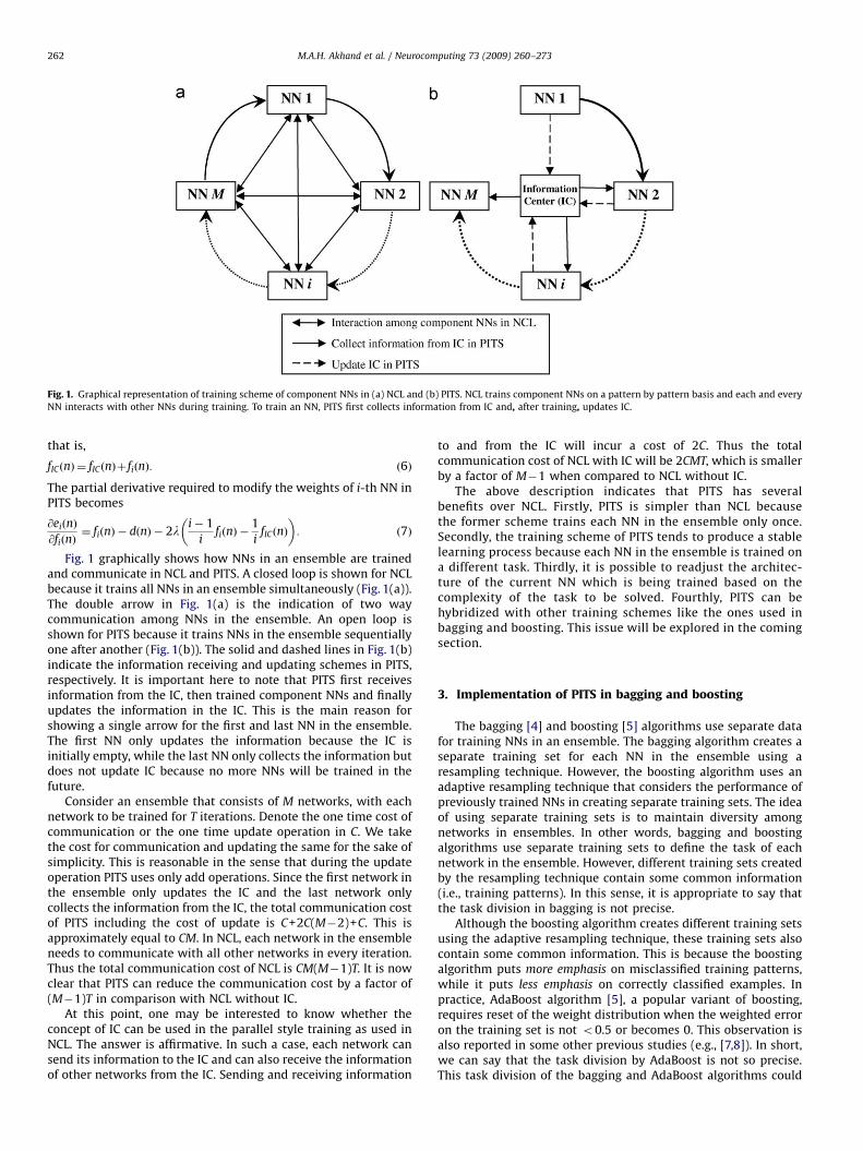
Fig. 1. Graphical representation of training scheme of component NNs in (a) NCL and (b) PITS. NCL trains component NNs on a pattern by pattern basis and each and every
NN interacts with other NNs during training. To train an NN, PITS first collects information from IC and, after training, updates IC.
M.A.H. Akhand et al. / Neurocomputing 73 (2009) 260–273262
that is,
fICðnÞ ¼ fICðnÞþ fiðnÞ: ð6Þ
The partial derivative required to modify the weights of i-th NN inPITS becomes
@eiðnÞ
@fiðnÞ¼ fiðnÞ � dðnÞ � 2l
i� 1
ifiðnÞ �
1
ifICðnÞ
� �: ð7Þ
Fig. 1 graphically shows how NNs in an ensemble are trainedand communicate in NCL and PITS. A closed loop is shown for NCLbecause it trains all NNs in an ensemble simultaneously (Fig. 1(a)).The double arrow in Fig. 1(a) is the indication of two waycommunication among NNs in the ensemble. An open loop isshown for PITS because it trains NNs in the ensemble sequentiallyone after another (Fig. 1(b)). The solid and dashed lines in Fig. 1(b)indicate the information receiving and updating schemes in PITS,respectively. It is important here to note that PITS first receivesinformation from the IC, then trained component NNs and finallyupdates the information in the IC. This is the main reason forshowing a single arrow for the first and last NN in the ensemble.The first NN only updates the information because the IC isinitially empty, while the last NN only collects the information butdoes not update IC because no more NNs will be trained in thefuture.
Consider an ensemble that consists of M networks, with eachnetwork to be trained for T iterations. Denote the one time cost ofcommunication or the one time update operation in C. We takethe cost for communication and updating the same for the sake ofsimplicity. This is reasonable in the sense that during the updateoperation PITS uses only add operations. Since the first network inthe ensemble only updates the IC and the last network onlycollects the information from the IC, the total communication costof PITS including the cost of update is C+2C(M�2)+C. This isapproximately equal to CM. In NCL, each network in the ensembleneeds to communicate with all other networks in every iteration.Thus the total communication cost of NCL is CM(M�1)T. It is nowclear that PITS can reduce the communication cost by a factor of(M�1)T in comparison with NCL without IC.
At this point, one may be interested to know whether theconcept of IC can be used in the parallel style training as used inNCL. The answer is affirmative. In such a case, each network cansend its information to the IC and can also receive the informationof other networks from the IC. Sending and receiving information
to and from the IC will incur a cost of 2C. Thus the totalcommunication cost of NCL with IC will be 2CMT, which is smallerby a factor of M�1 when compared to NCL without IC.
The above description indicates that PITS has severalbenefits over NCL. Firstly, PITS is simpler than NCL becausethe former scheme trains each NN in the ensemble only once.Secondly, the training scheme of PITS tends to produce a stablelearning process because each NN in the ensemble is trained ona different task. Thirdly, it is possible to readjust the architec-ture of the current NN which is being trained based on thecomplexity of the task to be solved. Fourthly, PITS can behybridized with other training schemes like the ones used inbagging and boosting. This issue will be explored in the comingsection.
3. Implementation of PITS in bagging and boosting
The bagging [4] and boosting [5] algorithms use separate datafor training NNs in an ensemble. The bagging algorithm creates aseparate training set for each NN in the ensemble using aresampling technique. However, the boosting algorithm uses anadaptive resampling technique that considers the performance ofpreviously trained NNs in creating separate training sets. The ideaof using separate training sets is to maintain diversity amongnetworks in ensembles. In other words, bagging and boostingalgorithms use separate training sets to define the task of eachnetwork in the ensemble. However, different training sets createdby the resampling technique contain some common information(i.e., training patterns). In this sense, it is appropriate to say thatthe task division in bagging is not precise.
Although the boosting algorithm creates different training setsusing the adaptive resampling technique, these training sets alsocontain some common information. This is because the boostingalgorithm puts more emphasis on misclassified training patterns,while it puts less emphasis on correctly classified examples. Inpractice, AdaBoost algorithm [5], a popular variant of boosting,requires reset of the weight distribution when the weighted erroron the training set is not o0.5 or becomes 0. This observation isalso reported in some other previous studies (e.g., [7,8]). In short,we can say that the task division by AdaBoost is not so precise.This task division of the bagging and AdaBoost algorithms could
ARTICLE IN PRESS
M.A.H. Akhand et al. / Neurocomputing 73 (2009) 260–273 263
be made more precise if training time interaction were introducedin these algorithms. The aim of this section is to explore this issue.
The proposed PITS is incorporated in bagging and AdaBoost toestablish training time interaction among NNs in the ensemble.We call the new schemes interactive bagging and interactiveAdaBoost. The interactive bagging algorithm is the hybridizationof bagging and PITS, while the interactive AdaBoost algorithm isthe hybridization of AdaBoost and PITS. The aim of this
Fig. 2. Interactive ba
Fig. 3. Interactive Ada
hybridization is to increase the diversity, i.e., reduce the overlap,in different networks of ensembles trained by the bagging andAdaBoost algorithms.
Figs. 2 and 3 show the pseudo codes for interactive baggingand interactive AdaBoost algorithms, respectively. The bold-facelines in these figures indicate the modifications/additions to thestandard bagging and AdaBoost algorithms. In interactive baggingor AdaBoost, the i-th NN is trained on a training set Ti created by
gging algorithm.
Boost algorithm.
ARTICLE IN PRESS
M.A.H. Akhand et al. / Neurocomputing 73 (2009) 260–273264
the bagging or AdaBoost algorithm, and the weight of this NN isupdated according to Eq. (7). It is seen from Eq. (7) that we need toknow the combined outputs of other NNs in the ensemble toupdate the weights of the i-th NN. Thus each network ininteractive bagging and AdaBoost collects the combined outputsof other NNs from the IC. This is a kind of indirect interactionamong networks in the ensemble which is not present in thestandard bagging and AdaBoost algorithms. After training anetwork, the interactive bagging and AdaBoost algorithmsupdate the information in the IC according to Eq. (6) for eachpattern in the original training set. This is an additional step,which is also not present in the standard bagging and AdaBoostalgorithms. It is now clear that the hybridization PITS withbagging/AdaBoost introduces two additional steps, i.e., communi-cation with the IC and updating the IC.
Recently, Liu [20,21] used bagging to create different trainingsets for training NNs in ensembles. In [20,21], each training set isused for training all NNs in the ensemble one time using NCL. Theaim of using separate training sets is to use them for the cross-validation purpose. However, in this study, PITS is employed toestablish training time interaction among the NNs in ensembleswhen they are trained in bagging.
4. Experimental studies
The PITS was applied along with BP and NCL to a suite of20 benchmark classification problems for observing the perfor-mance of the progressive training and indirect communicationschemes in constructing ensembles. The PITS was also comparedwith AdaBoost and DECORATE on the basis of their achievedperformance. Finally, the effect of different parameters on theperformance of NCL and PITS, and the performance of bagging andAdaBoost introducing PITS in their training processes wereinvestigated.
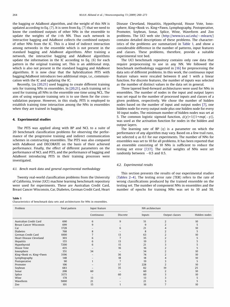
4.1. Bench mark data and general experimental methodology
Twenty real-world classification problems from the Universityof California, Irvine (UCI) machine learning benchmark repositorywere used for experiments. These are Australian Credit Card,Breast Cancer Wisconsin, Car, Diabetes, German Credit Card, Heart
Table 1Characteristics of benchmark data sets and architectures for NNs in ensembles.
Problem Total pattern Input feature
Continuous
Australian Credit Card 690 6
Breast Cancer Wisconsin 699 9
Car 1728 –
Diabetes 768 8
German Credit Card 1000 7
Heart Disease Cleveland 303 6
Hepatitis 155 6
Hypothyroid 7200 6
House Vote 435 –
Ionosphere 351 34
King+Rook vs. King+Pawn 3196 –
Lymphography 148 –
Postoperative 90 1
Promoter 106 –
Soybean 683 –
Sonar 208 60
Splice 3175 –
Wine 178 13
Waveform 5000 21
Zoo 101 15
Disease Cleveland, Hepatitis, Hypothyroid, House Vote, Iono-sphere, King+Rook vs. King+Pawn, Lymphography, Postoperative,Promoter, Soybean, Sonar, Splice, Wine, Waveform and Zooproblems. The UCI web site (http://www.ics.uci.edu/�mlearn/)contains detailed descriptions of these problems. The character-istics of the problems are summarized in Table 1, and show aconsiderable difference in the number of patterns, input featuresand classes. These problems, therefore, provide a suitableexperimental test bed.
The UCI benchmark repository contains only raw data thatrequire preprocessing to use in any NN. We followed thebenchmark methodology suggested in [16] for preprocessing thedata sets of different problems. In this work, the continuous inputfeature values were rescaled between 0 and 1 with a linearfunction. For discrete features, the number of inputs was selectedas the number of distinct values in the data set in general.
Three layered feed-forward architectures were used for NNs inensembles. The number of nodes in the input and output layerswas set equal to the number of processed inputs and classes of agiven problem, respectively. We chose the number of hiddennodes based on the number of input and output nodes [7], onehidden node for every output node plus one hidden node for every10 input nodes. The minimum number of hidden nodes was set at5. The common logistic sigmoid function, f(y)=1/(1+exp(�y)),was used as the activation function for nodes in the hidden andoutput layers.
The learning rate of BP (Z) is a parameter on which theperformance of any algorithm may vary. Based on a few trail runs,we selected Z as 0.1 for our experiments. The number of NNs forensembles was set to 10 for all problems. It has been reported thatan ensemble consisting of 10 NNs is sufficient to reduce thetesting set error [7,17]. The initial weights of NNs were setrandomly between �0.5 and 0.5.
4.2. Experimental results
This section presents the results of our experimental studies(Tables 2–4). The testing error rate (TER) refers to the rate ofwrong classifications produced by the trained ensemble on thetesting set. The number of component NNs in ensembles and thenumber of epochs for training NNs was set to 10 and 50,
The value in the bracket represents standard deviation. For statistical significance, single star (*) and double star (**) are for confidence interval 95% and 99%, respectively.
Table 3Testing error rate (TER) comparison among BP, NCL and PITS over five standard 10-fold cross validation runs.
Problem TER t-Test
BP NCL PITS BP vs. NCL BP vs. PITS NCL vs. PITS
Australian Card 0.1513(0.0415) 0.1449(0.0412) 0.1388(0.0444) *
Breast Cancer 0.0333(0.0286) 0.0322(0.0296) 0.0302(0.0275) * ** *
The value in the bracket represents standard deviation. For statistical significance, single star (*) and double star (**) are for confidence interval 95% and 99%, respectively.
M.A.H. Akhand et al. / Neurocomputing 73 (2009) 260–273 265
respectively. It was observed that a minimum TER was foundwith a particular value of l for both NCL and PITS. This value wasfound not to be the same for all problems. We, therefore, selectedthe value of l for a particular problem after some trial runs. Thisvalue was selected in the range of 0.25–0.75. It was done withthe hope that neither the performance of PITS nor NCL would beaffected by the value of l. The other parameters were chosen asdescribed in the experimental methodology section. For eachproblem, the best TER among the three methods is shown inbold-face type. Pair two tailed t-test was conducted to determinethe significance in the variation of results. If a result is foundsignificant by t-test, it is marked with a star (*). A single starmeans the TER difference is statistically significant with 95%confidence interval and a double star is for 99% confidenceinterval.
Table 2 represents the average results of ensembles producedby BP, NCL and PITS over 20 independent runs. In each run, two-thirds of the available examples were used for training and onethird for testing. The performance of ensembles trained by BP isthe worst when compared to the other two methods on 18 out of20 problems. Since we have used the same learning rate andinitial weights for BP, NCL and PITS, the performance differencebetween BP and NCL/PITS can be considered to be due to thetraining time interaction. This is because the basic differencebetween BP and NCL/PITS is the penalty term by which networkscan communicate with each other during training. In other words,the poor performance of BP is due to its independent trainingstrategy where component networks cannot communicate duringtraining [11,12]. However, the performance of BP, NCL and PITS isfound to be similar for Hepatitis and Postoperative problems that
ARTICLE IN PRESS
Table 4Testing error rate (TER) comparison among PITS, AdaBoost and DECORATE over five standard 10-fold cross validation runs.
Problem TER t-Test
PITS AdaBoost DECORATE PITS vs. AdaBoost PITS vs. DECORATE
Australian Card 0.1388(0.0444) 0.158(0.0426) 0.1406(0.0351) **
Breast Cancer 0.0302(0.0275) 0.0348(0.0284) 0.031(0.0284) **
The value in the bracket represents standard deviation. For statistical significance, single star (*) and double star (**) are for confidence interval 95% and 99%, respectively.
M.A.H. Akhand et al. / Neurocomputing 73 (2009) 260–273266
contain only 155 and 90 patterns, respectively. The training timeinteraction, which is used for producing diverse NNs, might nothelp for these problems. This is because each NN in the ensembleneeds a minimum amount of information to learn a problem. Thet-test indicated that the performance of ensembles trained by NCLand PITS is significantly better than that trained by BP on 9 and 15problems, respectively.
From Table 2 it can be seen that PITS performed better thanNCL on 14 out of 20 problems, while NCL outperformed PITS onthree problems. The two algorithms achieved similar performanceon three problems. The t-test shows that the performance of PITSwas significantly better than NCL on 11 problems. NCL, however,significantly outperformed PITS on two problems. These resultsindicate the essence of using the sequential training with trainingtime interaction for training NNs in ensembles.
A different arrangement of patterns in training and testing setsmay produce different performance, even when the number ofpatterns are kept the same for the training and testing sets. A newset of experiments has been carried out to observe performanceon the arrangement of patterns in the training and testing sets.Ten-fold cross validation was used for creating the training andtesting sets with different arrangement of patterns. In 10-foldcross validation, the patterns of the original data set were dividedinto 10 equal or nearly equal sets. By rotation, one set wasreserved for testing while the remaining nine sets were used fortraining.
Table 3 represents the average TERs of ensembles trained byBP, NCL and PITS for 20 problems over five standard 10-fold crossvalidation runs. According to Table 3, PITS is the best and BP is theworst among the three methods. BP achieved the same TER as NCLor PITS for only one problem (i.e., Postoperative), which consists ofa small number of patterns. PITS achieved the lowest TERs for 15problems, while NCL achieved the lowest TERs for three problems.The performance of NCL and PITS was found to be the same fortwo problems. t-test showed that NCL and PITS were significantlybetter than BP for six and 10 problems, respectively. PITS wasfound significantly better than NCL for five problems, while itwas not significantly outperformed by NCL for any problem. Inshort, PITS was found better or at least competitive with respect toNCL when applied to classification problems under differentconditions.
Although PITS is shown to achieve better performance overNCL, it is important to compare its performance with otherpopular or recently introduced ensemble method(s). Bagging andAdaBoost are among the most popular ensemble methods. Theproposed PITS has some similarities with AdaBoost in the sensethat both methods sequentially train networks for an ensemble.We therefore compare here PITS with AdaBoost. In addition, wecompare PITS with a recently introduced ensemble methodDECORATE.
Table 4 represents the average TERs of ensembles trained byPITS, AdaBoost and DECORATE over five standard 10-fold crossvalidation runs. The results for PITS are taken from Table 3. Tomake similarity, 10 networks were trained for an ensemble inAdaBoost. To be comparable to PITS and AdaBoost, the maximumnumber of networks per ensemble in DECORATE was defined as 10and maximum trial networks as 15. The performance ofDECORATE is also depends on its parameter value RSize, the ratioof diversity set to original training set. The results presented forDECORATE in Table 4 was the best result obtained by varying RSize
values from 0.5 to 1.0.According to Table 4, the overall performances of PITS are
better than AdaBoost and DECORATE as well. PITS achieved better(i.e., lower) TER than AdaBoost for 13 out of 20 problems, whileAdaBoost outperformed PITS on the remaining seven problems.The t-test shows that the performance of PITS was foundsignificantly better than AdaBoost on 10 problems, whileAdaBoost was found significantly better than PITS on fourproblems. On the other hand, PITS achieved better TER for 15problems when compared with DECORATE; among them forseven cases results were found significantly better by t-test. WhileDECORATE achieved lower TER than PITS for four problems. Theperformance of PITS and DECORATE was found to be the same forHeart Disease problem. It is now understood that PITS is better orat least competitive with respect to AdaBoost and DECORATE.
4.3. Experimental analyses
Since both NCL and PITS have maintained training timeinteraction, this section investigates the effect of differentparameters on the performance of NCL and PITS. We have
ARTICLE IN PRESS
M.A.H. Akhand et al. / Neurocomputing 73 (2009) 260–273 267
measured the competition among networks in ensembles andpresented effect of interaction styles of NCL and PITS on trainingtime of ensembles. In addition, we have shown the effect of noiseon the performance of PITS. We selected three problems, i.e.,Australian Card, Car and Waveform, for these analyses. Theseproblems were selected because they contain different types offeatures. For example, Australian Card problem contains bothcontinuous and discrete features, Car problem contains onlydiscrete features, and Waveform problem contains only contin-uous features.
Three parameters were varied to observe their effect on NCLand PITS. They were the size of the ensemble, the number ofiterations used for training NNs in ensembles and the penaltyterm factor l. For each data set, two-thirds of the examples wereused for training, while the remaining one-third was reserved fortesting.
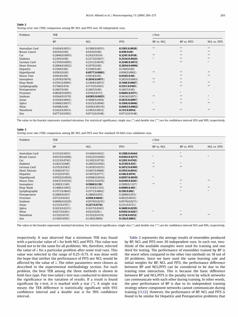
4.3.1. Effect of ensemble size
This section investigates empirically the effect of ensemblesize on its TER. For proper observation, the number of iterationsfor training each component NN was fixed at 50 and the value of lwas fixed at 0.5. The same parameter set was used for both NCLand PITS for a fair comparison.
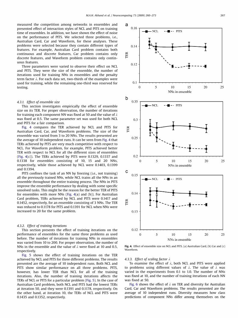
Fig. 4 compares the TER achieved by NCL and PITS forAustralian Card, Car, and Waveform problems. The size of theensemble was varied from 3 to 20 NNs. The results presented arethe average of 10 independent runs. It can be seen from Fig. 4 thatTERs achieved by PITS are very much competitive with respect toNCL. For Waveform problem, for example, PITS achieved betterTER with respect to NCL for all the different sizes of ensembles(Fig. 4(c)). The TERs achieved by PITS were 0.1329, 0.1337 and0.1338 for ensembles consisting of 10, 15 and 20 NNs,respectively, while those achieved by NCL were 0.1403, 0.1399and 0.1394.
PITS confines the task of an NN by freezing (i.e., not training)all the previously trained NNs, while NCL trains all the NNs in anensemble throughout the entire training process. The NNs in PITSimprove the ensemble performance by dealing with some specificunsolved tasks. This might be the reason for the better TER of PITSfor ensembles with more NNs (Fig. 4(a) and (b)). For AustralianCard problem, TERs achieved by NCL and PITS were 0.1417 and0.1452, respectively, for an ensemble consisting of 3 NNs. The TERwas reduced to 0.1178 for PITS and 0.1391 for NCL when NNs wereincreased to 20 for the same problem.
Fig. 4. Effect of ensemble size on NCL and PITS. (a) Australian Card, (b) Car and (c)
Waveform.
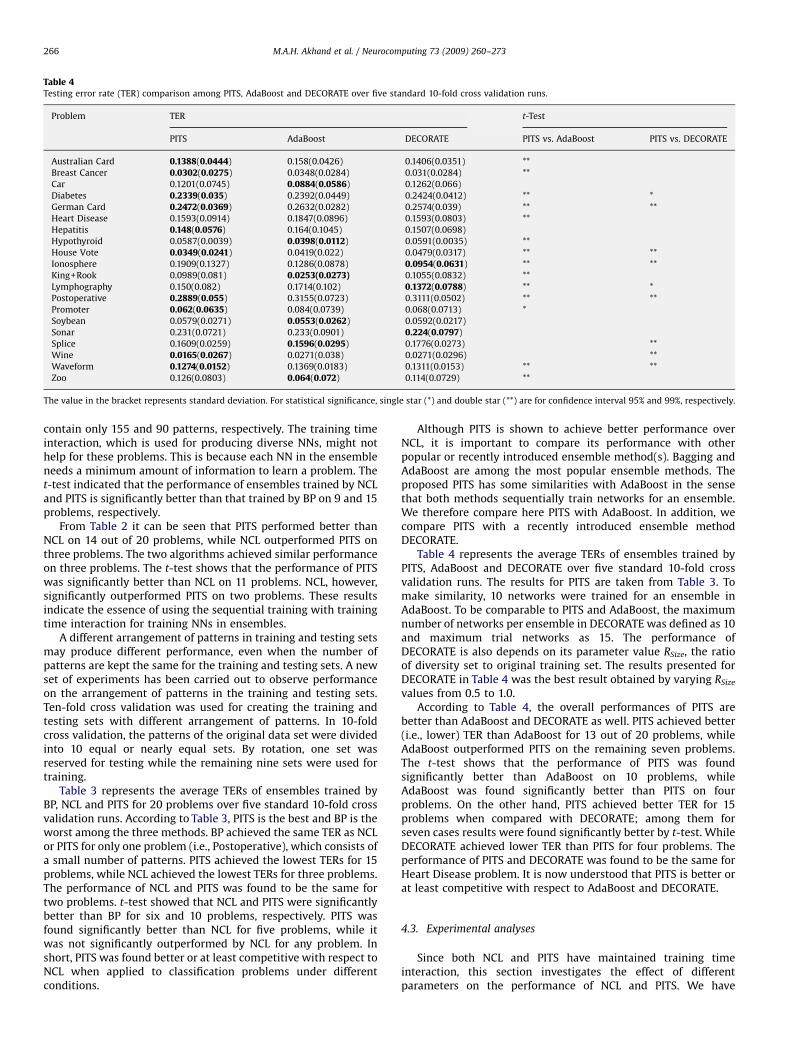
4.3.2. Effect of training iterations
This section presents the effect of training iterations on theperformance of ensembles for the same three problems as usedbefore. The number of iterations for training NNs in ensembleswas varied from 10 to 200. For proper observation, the number ofNNs in the ensemble and the value of l were fixed at 10 and 0.5,respectively.
Fig. 5 shows the effect of training iterations on the TERachieved by NCL and PITS for three different problems. The resultspresented are the average of 10 independent runs. Both NCL andPITS show similar performance on all three problems. PITS,however, has lower TER than NCL for all of the trainingiterations. Also, the number of training iterations affects theTERs of NCL or PITS for a particular problem (Fig. 5). In the case ofAustralian Card problem, both NCL and PITS had the lowest TERsat iteration 50, and they were 0.1391 and 0.1178, respectively. Onthe other hand, at iteration 10, the TERs of NCL and PITS were0.1435 and 0.1352, respectively.
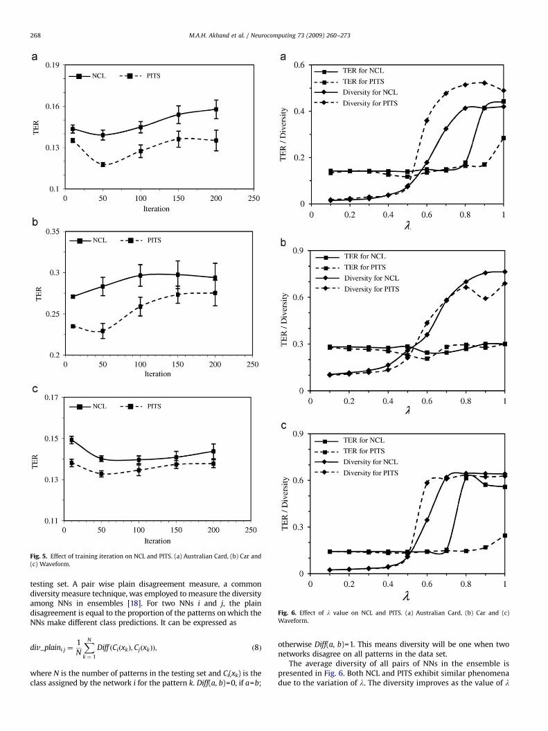
4.3.3. Effect of scaling factor lTo examine the effect of l, both NCL and PITS were applied
to problems using different values of l. The value of l wasvaried in the experiments from 0.1 to 1.0. The number of NNswas fixed at 10, and the number of training iterations of each NNwas fixed at 50.
Fig. 6 shows the effect of l on TER and diversity for AustralianCard, Car and Waveform problems. The results presented are theaverage of 10 independent runs. Diversity measures how classpredictions of component NNs differ among themselves on the
ARTICLE IN PRESS
Fig. 5. Effect of training iteration on NCL and PITS. (a) Australian Card, (b) Car and
(c) Waveform.
Fig. 6. Effect of l value on NCL and PITS. (a) Australian Card, (b) Car and (c)
Waveform.
M.A.H. Akhand et al. / Neurocomputing 73 (2009) 260–273268
testing set. A pair wise plain disagreement measure, a commondiversity measure technique, was employed to measure the diversityamong NNs in ensembles [18]. For two NNs i and j, the plaindisagreement is equal to the proportion of the patterns on which theNNs make different class predictions. It can be expressed as
div_plaini:j ¼1
N
XN
k ¼ 1
Diff ðCiðxkÞ;CjðxkÞÞ; ð8Þ
where N is the number of patterns in the testing set and Ci(xk) is theclass assigned by the network i for the pattern k. Diff(a, b)=0, if a=b;
otherwise Diff(a, b)=1. This means diversity will be one when twonetworks disagree on all patterns in the data set.
The average diversity of all pairs of NNs in the ensemble ispresented in Fig. 6. Both NCL and PITS exhibit similar phenomenadue to the variation of l. The diversity improves as the value of l
ARTICLE IN PRESS
M.A.H. Akhand et al. / Neurocomputing 73 (2009) 260–273 269
increases. The accuracy of the ensemble, however, is not alwaysimproved by improvement of diversity. For Waveform problem,the TER of NCL and PITS at l=1 was 0.5591 and 0.246,respectively. However, both NCL and PITS achieved the lowestTERs at l=0.5. In general, a trade-off between TER and diversity isobserved for both NCL and PITS. A similar observation was alsomade in some previous studies (e.g., [22,23]).
Notice that PITS exhibits more stable generalization than NCLon some problems due to the variation of l (Figs. 6(a) and (c)). Forexample, for the Australian Card problem, TERs achieved by PITSat l=0.1 and l=1.0 were 0.1339 and 0.2844, respectively, whilethose achieved by NCL at l=0.1 and l=1.0 were 0.1417 and 0.4426,respectively.
4.3.4. Competition in ensemble
The Latin root for the verb ‘‘to compete’’ is ‘‘competere’’, whichmeans ‘‘to seek together’’. Competition can have both beneficialand detrimental effects. Many evolutionary biologists view inter-species and intra-species competition as the driving force ofadaptation and ultimately, evolution. On the negative side,competition may also lead to wasted (duplicated) effort, andthereby may reduce the chance for solving a problem satisfacto-rily. For example, when networks in an ensemble do the same job,the unsolved parts of a given problem may increase. Ouralgorithm, PITS, is supposed to reduce competition by itssequential strategy for training networks in ensembles. In thecontext of NN ensembles, component networks can be consideredto be engaging in competition when they do the same task eventhough they are supposed to perform different tasks. Thisproduces ‘‘overlap’’ which indicates that the same predictionproduced by different NNs can be used as a measure ofcompetition. The enhancement of overlap may increase the‘‘uncover’’, i.e., the unsolved parts of a given problem, resultingin an unsatisfactory solution of the problem.
Table 5 presents rate of overlap and rate of uncover achievedby NCL and PITS on three different problems for different l values.The rate of overlap refers to the rate of correct classificationproduced by all NNs for a particular pattern in the training/testingset. On the other hand, rate of uncover refers to the rate of wrongclassification produced by all NNs for a particular pattern in thetraining/testing set. The number of NNs in an ensemble was fixedat 10, and each NN was trained for 50 epochs. The resultspresented are the average of 10 independent runs.
From Table 5 it can be seen that larger l values produce loweroverlap and uncover for both NCL and PITS. However, PITS seemsto achieve lower overlap and uncover with respect to NCL for any
Table 5Comparison between NCL and PITS based on overlap and uncover for training and test
Problem Penalty
factor (l)
Training
NCL PITS
Rate of
overlap
Rate of
uncover
Rate of
overlap
Australian Card 0.25 0.8659 0.0954 0.853
0.50 0.7309 0.0309 0.7591
0.75 0.0433 0.0022 0.00
Car 0.25 0.9163 0.0089 0.9044
0.50 0.7964 0.0025 0.7077
0.75 0.0004 0.0055 0.00
Waveform 0.25 0.8357 0.0894 0.8319
0.50 0.7163 0.032 0.6771
0.75 0.00 0.0352 0.00
l value on both training and testing sets. For example, for theAustralian Card problem, when the value of l was set to 0.75, therate of overlap and rate of uncover achieved by NCL on thetraining set were 0.0433 and 0.0022, respectively. In contrast,these two values were zero for PITS. A similar better performanceby PITS was also observed on the testing set. The results presentedin Table 5 indicate that PITS can reduce competition amongnetworks in an ensemble. When the value of l was set large, PITSremoved the competition among networks in the ensemble. It isimportant here to note that a large value of l is not suitable for theperformance of PITS (Fig. 6). Thus we can say that a small amountof competition is suitable for better performance.
4.3.5. Effect of interaction on training time
This section investigates the effect of different interactionstyles of NCL and PITS on training time of ensembles. Since PITS isdeveloped from NCL, like NCL, PITS is also an extension of BP.Therefore, training time of BP is also considered here for betterunderstanding. BP incurs time for generating actual response in aforward pass and time for correcting weight values in a backwardpass. In case of NCL and PITS, both have forward pass as similar toBP. In the backward pass, NCL and PITS use Eqs. (4) and (7),respectively, extensions of BP. Others are similar in both NCL andPITS in the backward pass also. The Eqs. (4) and (7) are responsiblefor different interaction styles in NCL and PITS, respectively.Therefore, training time of an ensemble by NCL or PITS mayconsider as the training time of BP plus the time for interactionamong the networks; and the time difference in between NCL andPITS may consider for the different interaction styles of thesemethods.
Table 6 compares the ensemble training time of BP, NCL andPITS for Australian Card, Car, and Waveform problems for differentensemble sizes. The size of the ensemble was varied from 3 to 20NNs. The results presented are the average of 10 independentruns. Actual training times for any method depend on severalfactors such as machine and environment. For consistency and faircomparison, experiments were done in the same machine, that is,Sony Vaio VGN-CR90S (CPU: Intel Core2Duo 2.40 GHz, RAM:2.00 GB). We implemented the algorithms on Visual C++ under MSVisual Studio 2005 and the operating system was Windows VistaHome edition.
It can be seen from Table 6 that BP required the least timeand NCL took the most time among the three methods (i.e., BP,NCL and PITS) for any problem for all the different sizes ofensembles. On the other hand, PITS took time in between BP andNCL. For example, BP, NCL and PITS took 12.399, 13.394, and
ing sets.
Testing
NCL PITS
Rate of
uncover
Rate of
overlap
Rate of
uncover
Rate of
overlap
Rate of
uncover
0.0685 0.8352 0.1278 0.8278 0.0996
0.0298 0.7604 0.07 0.7617 0.057
0.00 0.0483 0.0043 0.00 0.00
0.0062 0.6217 0.1816 0.6309 0.1773
0.0002 0.4589 0.1031 0.4884 0.0757
0.0001 0.0002 0.0077 0.00 0.003
0.0848 0.8167 0.1034 0.8117 0.0996
0.0243 0.6845 0.0439 0.6462 0.0332
0.0041 0.00 0.0361 0.00 0.0051
ARTICLE IN PRESS
Table 6Training time comparison among BP, NCL and PITS.
Problem NNs/ensemble Training time in seconds
BP NCL PITS
Australian Card 3 0.6754 0.7325 0.7193
5 1.1794 1.2151 1.2088
10 2.4147 2.5676 2.5118
15 3.4894 3.5287 3.5065
20 4.6724 4.8189 4.7455
Car 3 1.0608 1.1107 1.0857
5 1.7457 1.847 1.7972
10 3.5585 3.8249 3.702
15 5.3105 5.5225 5.4806
20 7.1431 7.4864 7.3008
Waveform 3 1.8096 1.9702 1.8719
5 3.0841 3.329 3.2152
10 6.1493 6.5691 6.5004
15 9.3133 9.9261 9.7405
20 12.399 13.3941 12.9947
Fig. 7. Effect of noise on the performance of PITS.
M.A.H. Akhand et al. / Neurocomputing 73 (2009) 260–273270
12.995 seconds, respectively, for Waveform problem whenensemble consisted of 20 NNs. Reason behind the less timerequirement by PITS than NCL is already explain Section 2, thatis, it trained first NN independently (like BP) and trained others,one after another, in conjunction with IC maintaining lessinteraction. On the other hand, in NCL all the NNs maintaineddirect interaction among themselves throughout the trainingprocess. In Table 6, the time difference between NCL and BP maybe considered as the interaction time for NCL, though time wasmeasured for different independent runs of NCL and BP.Similarly, PITS interaction time may be defined as the timedifference between PITS and BP. For the same Waveformproblem and ensemble of 20 networks, the interaction timefor NCL and PITS was then 0.995(=13.394–12.399) and0.596(=12.995–12.399) s, respectively.
From Table 6, it is found that time requirement of PITS was notmuch less than NCL, the reason is the common BP portion in bothcases that took more time than interaction. However, it isinteresting to observe the effect interaction style of PITS ontraining time of an ensemble when implemented in a machinewith one processor. Notice that the proposed PITS algorithm trainsall networks in an ensemble sequentially one after another, whileNCL trains them simultaneously pattern by pattern basis. There-fore, on a multi-processor machine NCL may get benefit fromparallel training of NNs and may perform faster than PITS. But insuch case synchronization among the NNs in the training schemeof NCL would be costly in terms of implementation and processingtime.
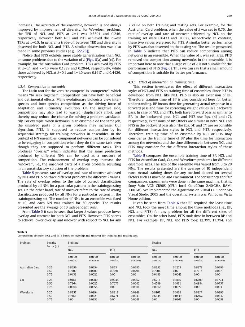
4.3.6. Effect of noise
The proposed PITS trains component networks in an ensemblesequentially as does the boosting algorithm. After training anetwork, the boosting algorithm changes the distribution oftraining patterns based on the trained network’s performanceowing to emphasize coming networks on previously misclassifiedpatterns. When a training set contains noise, boosting may focuson noise resulting in poor generalization [7,24]. Although PITSdoes not create different training sets by changing the distributionof training patterns, it is interesting to know the effect of noise onthe performance of PITS.
To observe the effect of noise on PITS, we first create a noisytraining set by adding Gaussian noise with a mean of zero and astandard deviation of one to the original training set. Then wetrained component networks in an ensemble on the noisy training
set using PITS. The noise is added to the input attributes or thetarget outputs of the training set. We also create a noisy trainingset by randomly altering the class labels of the patterns in thetraining set.
Fig. 7 presents the effect of noise on PITS for Waveformproblem where X% indicates the percent of training patternschanged by adding noise or switching class labels. It is worthmentioning here that 0% noise means a training set without noise,i.e., original training set. The presented results are the average of10 independent runs. For proper observation, the number of NNsin an ensemble was fixed at 10, each NN was trained for 50epochs, and the value of l was fixed at 0.5. From Fig. 7 it can beseen that the performance of PITS does not vary too much for asmall amount of noise in the input or output. After a certain limit,for example 30%, the effect of noise is found to be significant.These results indicate that PITS can tolerate a certain amount ofnoise.
4.4. Effect of PITS in bagging and AdaBoost
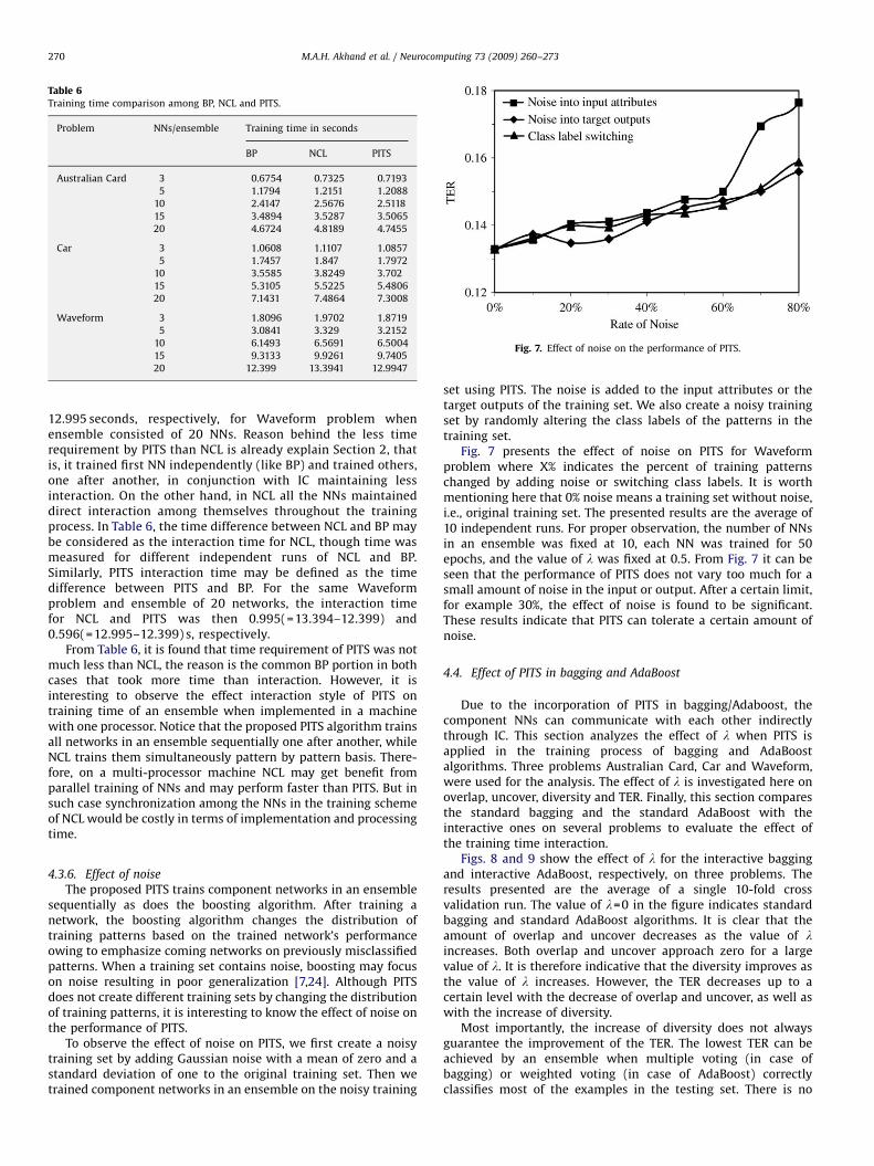
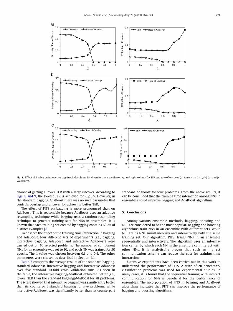
Due to the incorporation of PITS in bagging/Adaboost, thecomponent NNs can communicate with each other indirectlythrough IC. This section analyzes the effect of l when PITS isapplied in the training process of bagging and AdaBoostalgorithms. Three problems Australian Card, Car and Waveform,were used for the analysis. The effect of l is investigated here onoverlap, uncover, diversity and TER. Finally, this section comparesthe standard bagging and the standard AdaBoost with theinteractive ones on several problems to evaluate the effect ofthe training time interaction.
Figs. 8 and 9 show the effect of l for the interactive baggingand interactive AdaBoost, respectively, on three problems. Theresults presented are the average of a single 10-fold crossvalidation run. The value of l=0 in the figure indicates standardbagging and standard AdaBoost algorithms. It is clear that theamount of overlap and uncover decreases as the value of lincreases. Both overlap and uncover approach zero for a largevalue of l. It is therefore indicative that the diversity improves asthe value of l increases. However, the TER decreases up to acertain level with the decrease of overlap and uncover, as well aswith the increase of diversity.
Most importantly, the increase of diversity does not alwaysguarantee the improvement of the TER. The lowest TER can beachieved by an ensemble when multiple voting (in case ofbagging) or weighted voting (in case of AdaBoost) correctlyclassifies most of the examples in the testing set. There is no
ARTICLE IN PRESS
Fig. 8. Effect of l value on interactive bagging. Left column for diversity and rate of overlap, and right column for TER and rate of uncover. (a) Australian Card, (b) Car and (c)
Waveform.
M.A.H. Akhand et al. / Neurocomputing 73 (2009) 260–273 271
chance of getting a lower TER with a large uncover. According toFigs. 8 and 9, the lowest TER is achieved for lr0.5. However, inthe standard bagging/AdaBoost there was no such parameter thatcontrols overlap and uncover for achieving better TER.
The effect of PITS on bagging is more pronounced than onAdaBoost. This is reasonable because AdaBoost uses an adaptiveresampling technique while bagging uses a random resamplingtechnique to generate training sets for NNs in ensembles. It isknown that each training set created by bagging contains 63.2% ofdistinct examples [8].
To observe the effect of the training time interaction in baggingand AdaBoost, four different sets of experiments (i.e., bagging,interactive bagging, AdaBoost, and interactive AdaBoost) werecarried out on 10 selected problems. The number of componentNNs for an ensemble was set to 10, and each NN was trained for 50epochs. The l value was chosen between 0.1 and 0.4. The otherparameters were chosen as described in Section 4.1.
Table 7 compares the average results of the standard bagging,standard AdaBoost, interactive bagging and interactive AdaBoostover five standard 10-fold cross validation runs. As seen inthe table, the interactive bagging/AdaBoost exhibited better (i.e.,lower) TER than the standard bagging/AdaBoost for all problems.The t-test showed that interactive bagging was significantly betterthan its counterpart standard bagging for five problems, whileinteractive AdaBoost was significantly better than its counterpart
standard AdaBoost for four problems. From the above results, itcan be concluded that the training time interaction among NNs inensembles could improve bagging and AdaBoost algorithms.
5. Conclusions
Among various ensemble methods, bagging, boosting andNCL are considered to be the most popular. Bagging and boostingalgorithms train NNs in an ensemble with different sets, whileNCL trains NNs simultaneously and interactively with the sametraining set. Our algorithm, PITS, trains NNs in an ensemblesequentially and interactively. The algorithm uses an informa-tion center by which each NN in the ensemble can interact withother NNs. It is analytically proven that such an indirectcommunication scheme can reduce the cost for training timeinteraction.
Extensive experiments have been carried out in this work tounderstand the performance of PITS. A suite of 20 benchmarkclassification problems was used for experimental studies. Inmany cases, it is found that the sequential training with indirectcommunication for NNs is beneficial for the performance ofensembles. The incorporation of PITS in bagging and AdaBoostalgorithms indicates that PITS can improve the performance ofbagging and boosting algorithms.
ARTICLE IN PRESS
Fig. 9. Effect of l value on interactive AdaBoost. Left column for diversity and rate of overlap, and right column for TER and rate of uncover. (a) Australian Card, (b) Car and
(c) Waveform.
Table 7Comparison of testing error rate (TER) between the standard bagging (or standard AdaBoost) and the interactive bagging (or interactive AdaBoost) over five standard 10-fold
cross validation runs.
Problem Bagging AdaBoost
Standard Interactive (Bagging+PITS) Standard Interactive (AdaBoost+PITS)
Australian Card 0.1429(0.0404) 0.1313(0.0441)** 0.158(0.0426) 0.1406(0.0431)**
Car 0.1184(0.0663) 0.117(0.0645) 0.0884(0.0586) 0.0813(0.0525)
The value in the bracket represents standard deviation. For statistical significance, single star (*) and double star (**) are for confidence interval 95% and 99%, respectively.
M.A.H. Akhand et al. / Neurocomputing 73 (2009) 260–273272
There are several future potential directions that follow fromthis study. Firstly, though PITS trains NNs one after another,adjusting the parameter of coming NNs based on the combinedperformance of previously trained NNs might improve theperformance of PITS. Secondly, it is possible to determine thenumber of networks automatically for PITS. After training a
network and evaluating the current ensemble, it might be possibleto guess whether additional networks are necessary or not.Thirdly, since PITS is investigated for AdaBoost only in the presentstudy, the implementation of PITS as an element of interaction inother boosting algorithms, as well as other algorithms (e.g.,DECORATE), might be interesting.
ARTICLE IN PRESS
M.A.H. Akhand et al. / Neurocomputing 73 (2009) 260–273 273
Acknowledgments
This work was supported by Grants to KM from the JapaneseSociety for Promotion of Sciences (JSPS), the Yazaki MemorialFoundation for Science and Technology, and the University ofFukui. MMI was supported by the JSPS fellowship.
[3] G. Brown, J. Wyatt, R. Harris, X. Yao, Diversity creation methods: a survey andcategorization, Information Fusion 6 (2005) 99–111.
[4] L. Breiman, Bagging predictors, Machine Learning 24 (1996) 123–140.[5] Y. Freund, R.E. Schapire, Experiments with a new boosting algorithm, in:
Proceedings of the 13th International Conference on Machine Learning,Morgan Kaufmann, Los Altos, CA, 1996, pp. 148–156.
[6] J.R. Quinlan, Bagging, boosting, and C4.5, in: Proceedings of the 13th NationalConference on Artificial Intelligence and Eighth Innovative Applications ofArtificial Intelligence Conference, AAAI Press/MIT Press, Menlo Park, 1996,pp. 725–730.
[7] D.W. Opitz, R. Maclin, Popular ensemble methods: an empirical study, Journalof Artificial Intelligence Research 11 (1999) 169–198.
[8] E. Bauter, R. Kohavi, An empirical comparison of voting classificationalgorithms: bagging, boosting, and variants, Machine Learning 36 (1999)105–142.
[9] Md. Monirul Islam, X. Yao, K. Murase, A constructive algorithm for trainingcooperative neural network ensembles, IEEE Transactions on Neural Net-works 14 (2003) 820–834.
[10] G. Brown, Diversity in neural network ensembles, Ph.D. Thesis, School ofComputer Science, University of Birmingham, UK, 2003.
[11] Y. Liu, X. Yao, Simultaneous training of negatively correlated neural networksin an ensemble, IEEE Transactions on Systems, Man, and Cybernetics, Part B:Cybernetics 29 (6) (1999) 716–725.
[12] Y. Liu, X. Yao, Ensemble learning via negative correlation, Neural Networks 12(1999) 1399–1404.
[13] P. Melville, R.J. Mooney, Creating diversity in ensembles using artificial data,Information Fusion 6 (2005) 99–111.
[14] E. Bonabeau, M. Dorigo, G. Theraulaz, Swarm Intelligence: From Natural toArtificial Systems, Oxford University Press, Oxford, 1999.
[15] O. Cordon, F. Herrera, T. Stutzle, A review on the ant colony optimizationmetaheuristic: basis, models and new trends, Mathware and Soft Computing9 (2002) 141–175.
[16] L. Prechelt, Proben1—a set of benchmarks and benching rules for neuralnetwork training algorithms, Technical Report 21/94, Fakultat fur Informatik,University of Karlsruhe, Germany, 1994.
[17] K. Hansen, P. Salamon, Neural network ensembles, IEEE Transactions onPattern Analysis and Machine Intelligence 12 (10) (1990) 993–1001.
[18] A. Tsymbal, M. Pechenizkiy, P. Cunningham, Diversity in search strategies forensemble feature selection, Information Fusion 6 (2005) 83–98.
[19] S. Haykin, Neural Networks—A Comprehensive Foundation, third ed.,Prentice Hall, New York, 1999.
[20] Y. Liu, Generate different neural networks by negative correlation learning,Lecture Notes in Computer Science, vol. 3610, Springer, Berlin/Heidelberg,2005, pp. 149–156.
[21] Y. Liu, How to generate different neural networks, Studies in ComputationalIntelligence (SCI) 35 (2007) 225–240.
[22] A. Chandra, H. Chen, X. Yao, Trade-off between diversity and accuracy inensemble generation, Studies in Computational Intelligence (SCI) 16 (2006)429–464.
[23] L.I. Kuncheva, C.J. Whitaker, Measures of diversity in classifier ensembles,Machine Learning 51 (2003) 181–207.
[24] A. Vezhnevets, O. Barinova, Avoiding boosting overfitting by removingconfusing samples, Lecture Notes in Computer Science 4701 (2007) 430–441.
[25] T.K. Ho, The random subspace method for constructing decision forests, IEEETransactions on Pattern Analysis and Machine Intelligence 20 (1998)832–844.
M.A.H. Akhand received the B.E. degree in Electricaland Electronic Engineering from Khulna University ofEngineering and Technology (KUET), Bangladesh in1999, the M.E. degree in Human and Artificial Intelli-gence Systems in 2006, and the Doctoral degree inSystem Design Engineering in 2009 from University ofFukui, Japan. He joined as a lecturer at the Departmentof Computer Science and Engineering at KUET in 2001,and is now an Assistant Professor. He is a member ofthe Bangladesh Computer Society. His research interestincludes artificial neural networks and the applicationsto classification and on-line business systems.
Md. Monirul Islam received the B.E. degree inElectrical and Electronic Engineering from KhulnaUniversity of Engineering and Technology (KUET),Bangladesh, in 1989, the M.E. degree in ComputerScience and Engineering from Bangladesh University ofEngineering and Technology (BUET), Bangladesh, in1996, and the Doctoral degree in Evolutionary Roboticsfrom University of Fukui, Fukui, Japan, in 2002. From1989 to 2002, he was a Lecturer and Assistant Professorin the Department of Electrical and Electronic Engi-neering, KUET. In 2003, he moved to BUET as anAssistant Professor in the Department of Computer
Science and Engineering and now Associate Professor
of this department. Currently he is at the University of Fukui, Japan as a visitingAssociate Professor of Graduate School of Engineering, supported by the JapaneseSociety for the Promotion of Sciences. His research interests include evolutionaryrobotics, evolutionary computation, neural networks, and pattern recognition.
Kazuyuki Murase is a Professor at the Department ofHuman and Artificial Intelligence Systems, GraduateSchool of Engineering, University of Fukui, Fukui,Japan, since 1999. He received M.E. in ElectricalEngineering from Nagoya University in 1978, Ph.D. inBiomedical Engineering from Iowa State University in1983. He Joined as a Research Associate at Departmentof Information Science of Toyohashi University ofTechnology in 1984, as an Associate Professor at theDepartment of Information Science of Fukui Universityin 1988, and became the Professor in 1992. He is amember of The Institute of Electronics, Information
and Communication Engineers (IEICE), The Japanese
Society for Medical and Biological Engineering (JSMBE), The Japan NeuroscienceSociety (JSN), The International Neural Network Society (INNS), and The Society forNeuroscience (SFN). He serves as a Board of Directors in Japan Neural NetworkSociety (JNNS), a Councilor of Physiological Society of Japan (PSJ) and a Councilorof Japanese Association for the Study of Pain (JASP).