Project Final Report

EECE 5643 Simulation and Performance Evaluation Kaushik Padmanabhan, Chander Mohan, David Stewart

1

Analysis of Performance of Docker for

Varying I/O Intensive Workloads

(Project Report)

By,

Kaushik Padmanabhan

Chander Mohan

David Stewart


2

Table of Contents

Abstract………………………………………………………………………………………………………………………………………3 What is Docker?...............................................................................................................................3

Difference between VM-Ware and Docker…………………………………………………………...….3

Advantages…………………………………………………………………………………………...………4

Our Method…………………………………………………………………………………………………..4

Performance Analysis tools………………………………………………………………………………..5

Benchmarks…………………………………………………………………………,,,………......…….…..5

Considerations………………………………………………………………………………………………5

Process flow………………………………………………………………………………………..............6

Performance Metrics……………………………………………………………………………........…...6

Case 1: Total I/O Entries and Size comparison……………………….…………………….......6

Case 2: CPU Utilization…………………………………………………….………………………9

Case 3: Frequency of LBA Comparison………………………………….………………………10

Case 4: Sequential and Random Reads/Writes ratio variation……………………………… 11

Case 5: Read to Write ratio variation……………………………………………………………12

Conclusion…………………………………………………………………………………………………13

Future Work……………………………………………………………………………………………….13

Project Files……………………………………………………………………………………………….13

Acknowledgements………………………………………………………………………………………..13

Reference…………………………………………………………………………………………………..13

Table of Figures

Fig. 1: Docker illustration……………………………………………………………………………….…3

Fig. 2: Difference between VM and Docker.…………………………………………………………….4

Fig. 3: Total I/O entries in 1000 second time frame.....……………………………………………….7

Fig. 4: Total I/O size in 1000 second time frame……………………………………………………….7

Fig. 5: Total I/O size in 100 second time frame..…………………………………………………….…8

Fig. 6: Service Time in 100 second time frame...……………………………………………………….8

Fig. 7: Variation of tpmc for 3600 seconds…………………………………………………………….9

Fig. 8: CPU Utilization.………………………………………………………………………………….10

Fig. 9: Frequency of LBA Ratio..……………………………………………………………………….10

Fig. 10: Sequential I/O Access.…...…………………………………………………………………….11

Fig. 11: Random I/O Access...………………………………………………………………………….11

Fig. 12: Write Ratio Comparison...…………………………………………………………………….12

Fig. 13: Read Ratio Comparison...…………………………………………………………………….12

Fig. 14: Read/Write Ratio Comparison.……………………………………………………………….13


3

Abstract

Docker, an alternative for Virtual Machine, provides a way to run applications securely, isolated in

a container, packaged with all its dependencies and libraries. In this project, we are considering

homogenous instances of a particular application in Docker containers under that particular

application’s image, which can hold numerous records of data. Using this, we are going to evaluate

the optimum number of containers under the same application’s image which is adversely affected

by the number of records in numerous instances of an application within those containers.

Keywords – Docker Containers, Application, Performance Evaluation, Optimum Containers.

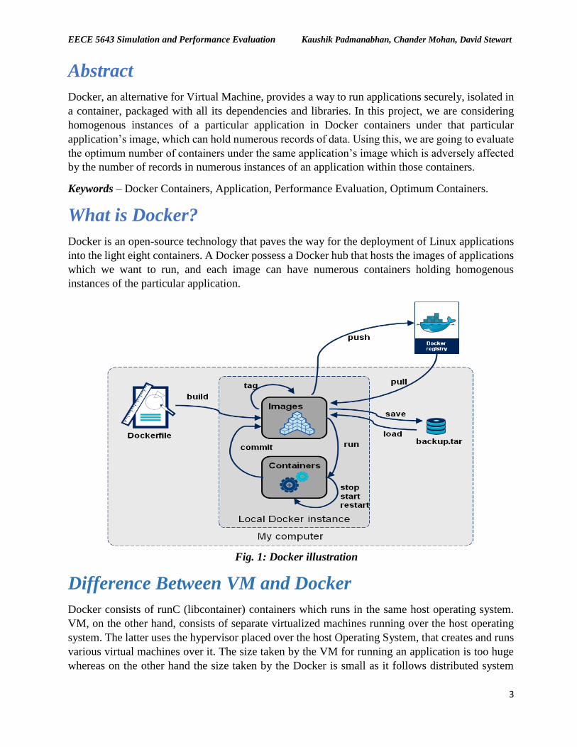
What is Docker?

Docker is an open-source technology that paves the way for the deployment of Linux applications

into the light eight containers. A Docker possess a Docker hub that hosts the images of applications

which we want to run, and each image can have numerous containers holding homogenous

instances of the particular application.

Fig. 1: Docker illustration

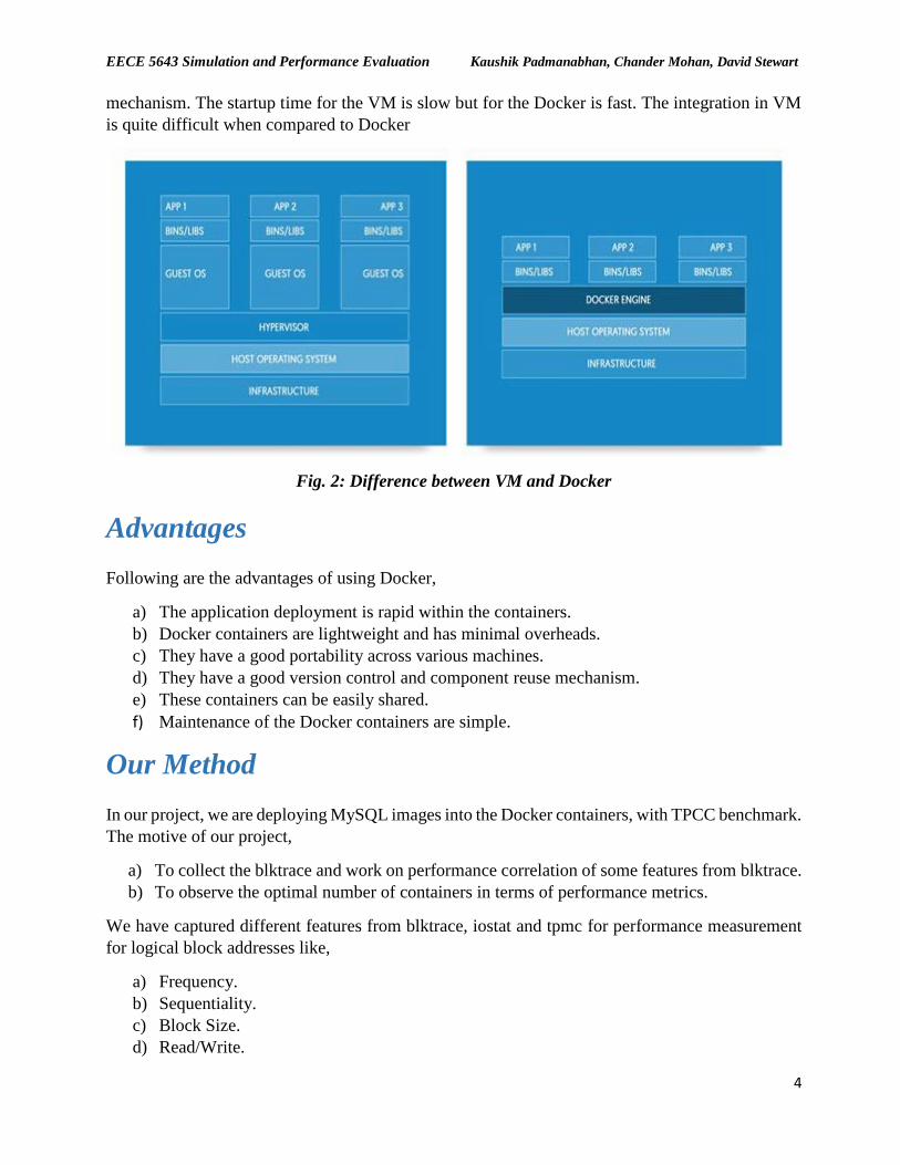
Difference Between VM and Docker

Docker consists of runC (libcontainer) containers which runs in the same host operating system.

VM, on the other hand, consists of separate virtualized machines running over the host operating

system. The latter uses the hypervisor placed over the host Operating System, that creates and runs

various virtual machines over it. The size taken by the VM for running an application is too huge

whereas on the other hand the size taken by the Docker is small as it follows distributed system


4

mechanism. The startup time for the VM is slow but for the Docker is fast. The integration in VM

is quite difficult when compared to Docker

Fig. 2: Difference between VM and Docker

Advantages

Following are the advantages of using Docker,

a) The application deployment is rapid within the containers.

b) Docker containers are lightweight and has minimal overheads.

c) They have a good portability across various machines.

d) They have a good version control and component reuse mechanism.

e) These containers can be easily shared.

f) Maintenance of the Docker containers are simple.

Our Method

In our project, we are deploying MySQL images into the Docker containers, with TPCC benchmark.

The motive of our project,

a) To collect the blktrace and work on performance correlation of some features from blktrace.

b) To observe the optimal number of containers in terms of performance metrics.

We have captured different features from blktrace, iostat and tpmc for performance measurement

for logical block addresses like,

a) Frequency.

b) Sequentiality.

c) Block Size.

d) Read/Write.


5

Performance Analysis Tools

In this project, we are analyzing the performance of Docker increasing containers. For measuring

this performance, we are using the following performance measuring tools which are then analyzed

to get the required result.

a) blktrace ‘blktrace’ is a block layer IO tracing mechanism which provides detailed information about

request queue operations up to user space. It is a utility which transfers event traces from

the kernel into either long-term on-disk storage, or provides direct formatted output (via

blkparse).

b) blkparse

‘blkparse’ is a utility which formats events stored in files, or when run in live mode directly

outputs data collected by blktrace.

c) iostat

‘iostat’ reports the Central Processing Unit (CPU) statistics and input/output statistics for

devices and partitions.

d) tpmc

‘tpmc’ gives details on the number of transactions taken place in a database per minute.

Benchmarks

The benchmark used to load automatically and analyze the performance of the MySQL databases

within the containers is TPC-C Benchmark. TPC-C is a write intensive test. We downloaded the

tpcc benchmark (tpcc_mysql_master) to load and measure the performance of MySQL. The two

operations that the TPC-C benchmark performs are,

a) tpcc_load – This will load the multiple records into the table without considering the

manual loading.

b) tpcc_start – This will start and run the database and measures the transactions happening

between the connections mentioned.

Considerations

For our project, we have considered 6 Containers and the major application image used is MySQL:

5.7. After importing the image and creating the containers, we ran the TPC-C benchmark in each

container for about,

Container1: ramp up time – 900 secs and measure time 3600 secs



6





While running the TPC-C start, we simultaneously ran the blktrace and got the results for 1000 secs

and ran iostat for about 100 secs.

Process Flow

We created containers and pulled MySQL images into the containers. Then we created the database

and imported ‘create_table.sql’ and ‘add_foreign_key.sql’ into the database. After importing the

tables into the database, we ran the tpcc_load command to load the data into the tables in each

container. We then ran the tpcc_start to start the execution of the tables which will measure the

number of transactions. Simultaneously, we measured the performance of the containers using

blktrace, blkparse and iostat commands.

Performance Metrics

The following performance metrics are considered for analyzing the optimum number of containers

required for running a Docker over the host Operating System,

a) Total I/O entries and size variation with respect to increasing Containers. Measured form

blktrace, blkparse and iostat.

b) CPU Utilization with respect to increasing Containers. Measured form iostat.

c) Frequency of Logical Block Addressing with respect to increasing Containers. Measured

form blktrace and blkparse.

d) Sequential and Random Reads/Writes percentage variation with respect to increasing

Containers. Measured form blktrace and blkparse.

e) Read to Write ratio variation with respect to increasing Containers. Measured form

blktrace and blkparse.

Case 1: Total I/O Entries and Size Comparison

After getting the blktrace, ran for 1000 seconds, and iostat results, ran for 100 seconds, we

developed an algorithm to measure the performance metrics. From these results ran for different

container, we got a result on number of I/O entries that happened within that 1000 second time

frame. We also analyzed the size of the I/O entries that happened within that 1000 second time

frame.


7

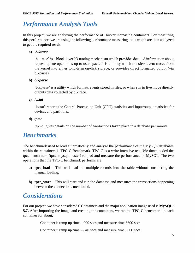
a) Using blktrace

Fig. 3: Total I/O entries in 1000 second time frame

From Fig.3, it is evident that the number of I/O entries increase with respect to increase in number

of containers and reach the peak for the number of containers to be equal to 3. Then after that, the

I/O entries obtained using blktrace for a time frame of 1000 seconds decrease and gets saturated

with the increase in containers.

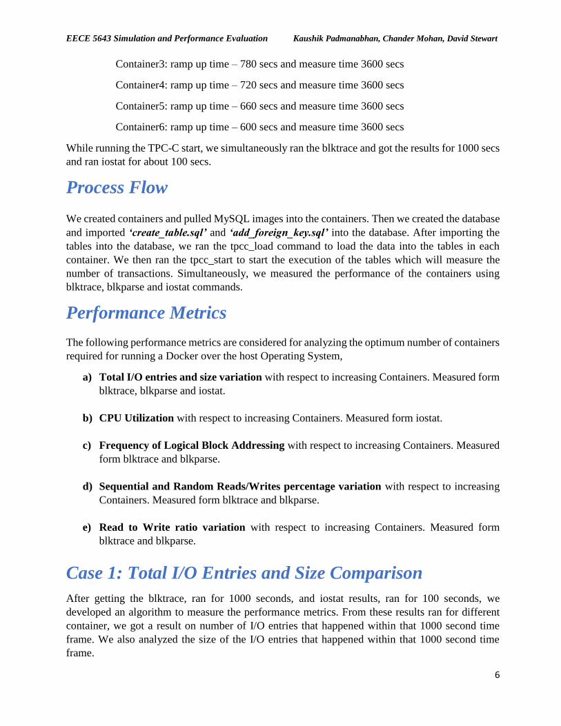
Fig. 4: Total I/O size in 1000 second time frame

The same happening, as in case of Fig. 3, is seen in Fig. 4, which reveals the I/O size variation with

respect to increase in the number of containers. As the containers increase, the I/O size varies and

increases and reach the peak for the number of containers to be equal to 3. It gets saturated after

that. The above happening can be analyzed using iostat results obtained. We considered the results

of iostat in order to get a detailed analysis on why the change happened at the CPU level, with

respect to the number of I/O entries as the number of containers increase

412859 440947 447577 431115 432504 431306

1

100001

200001

300001

400001

500001

1 2 3 4 5 6

Nu

mb

er o

f I/

O E

ntr

ies

No. of Containers

Total number of I/O Entries

2129176022986336 23130872 22681392 22737824 22608464

1

5000001

10000001

15000001

20000001

25000001

1 2 3 4 5 6

Size

in B

ytes

No. of Containers

Total I/O size


8

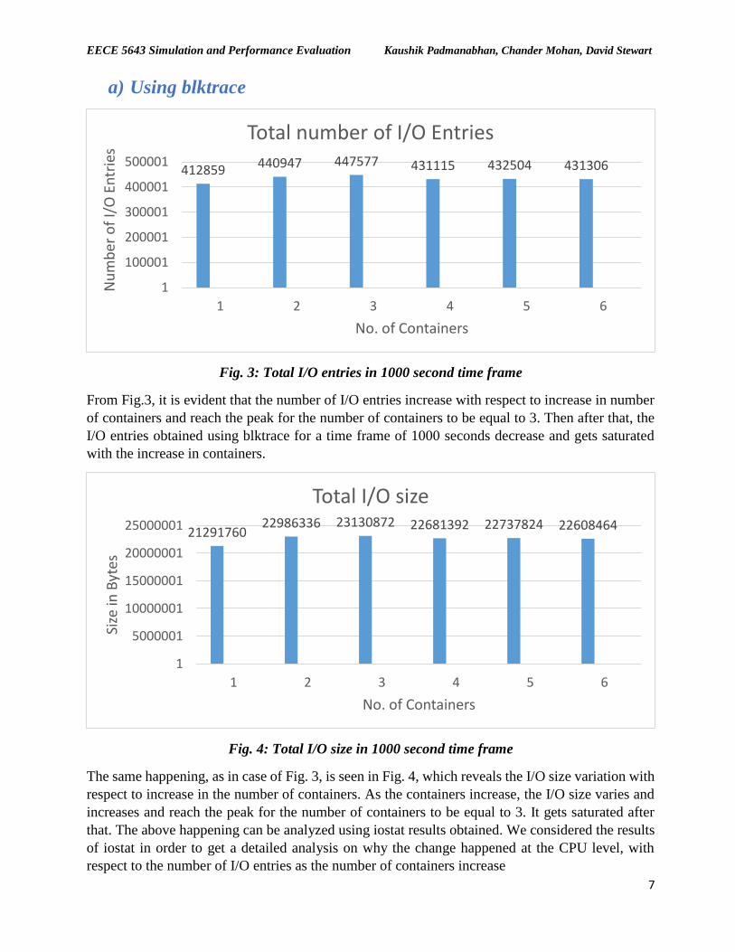
b) Using iostat

From Fig. 5, which refers to the size of the I/O entries calculated by iostat for 100 seconds, it is

evident that, the number of entries increase till the container size is 3 and gets saturated after that.

Fig. 5: Total I/O size in 100 second time frame

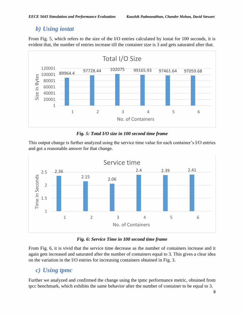
This output change is further analyzed using the service time value for each container’s I/O entries

and got a reasonable answer for that change.

Fig. 6: Service Time in 100 second time frame

From Fig. 6, it is vivid that the service time decrease as the number of containers increase and it

again gets increased and saturated after the number of containers equal to 3. This gives a clear idea

on the variation in the I/O entries for increasing containers obtained in Fig. 3.

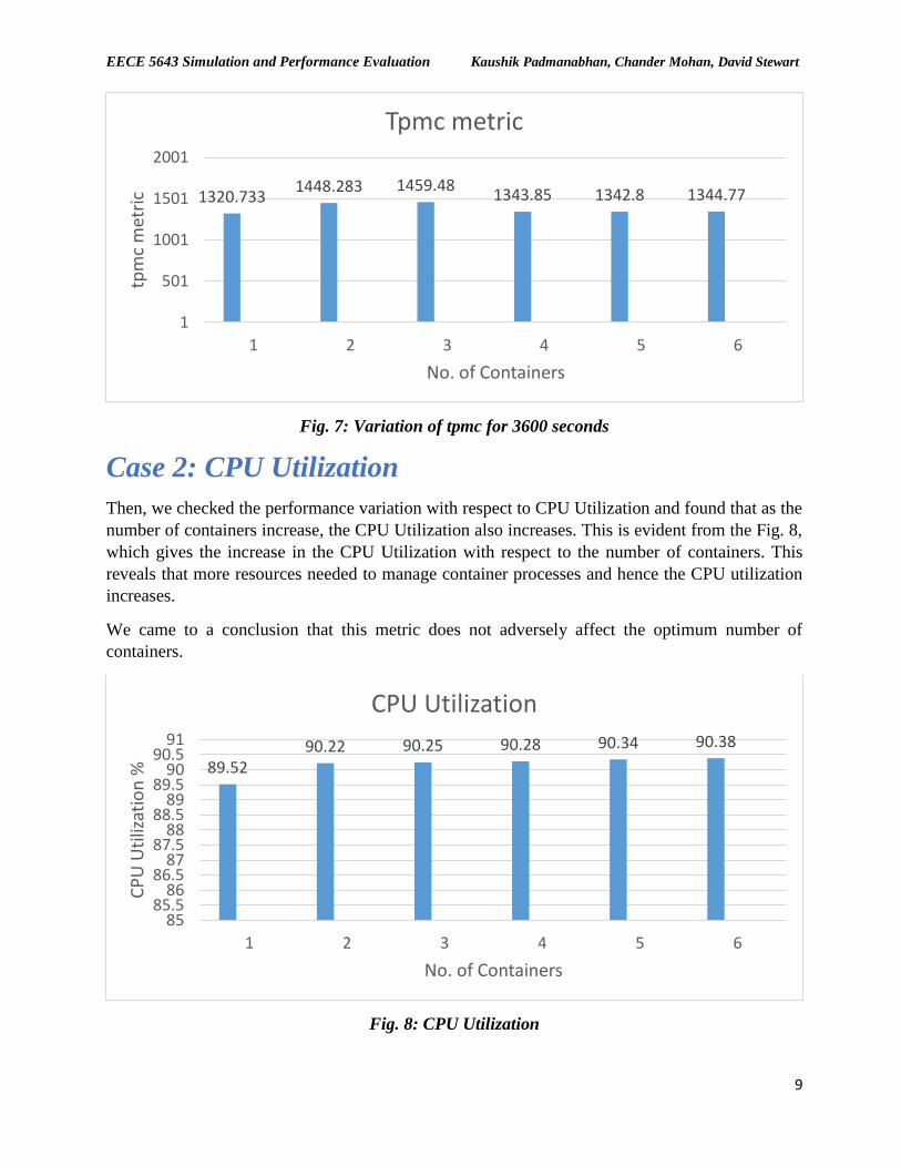
c) Using tpmc

Further we analyzed and confirmed the change using the tpmc performance metric, obtained from

tpcc benchmark, which exhibits the same behavior after the number of container to be equal to 3.

89964.497728.44 102075 99165.93 97461.64 97059.68

1

20001

40001

60001

80001

100001

120001

1 2 3 4 5 6

Size

in B

ytes

No. of Containers

Total I/O Size

2.362.15 2.06

2.4 2.39 2.41

1

1.5

2

2.5

1 2 3 4 5 6

Tim

e in

Sec

on

ds

No. of Containers

Service time


9

Fig. 7: Variation of tpmc for 3600 seconds

Case 2: CPU Utilization

Then, we checked the performance variation with respect to CPU Utilization and found that as the

number of containers increase, the CPU Utilization also increases. This is evident from the Fig. 8,

which gives the increase in the CPU Utilization with respect to the number of containers. This

reveals that more resources needed to manage container processes and hence the CPU utilization

increases.

We came to a conclusion that this metric does not adversely affect the optimum number of

containers.

Fig. 8: CPU Utilization

1320.7331448.283 1459.48

1343.85 1342.8 1344.77

1

501

1001

1501

2001

1 2 3 4 5 6

tpm

c m

etri

c

No. of Containers

Tpmc metric

89.5290.22 90.25 90.28 90.34 90.38

8585.5

8686.5

8787.5

8888.5

8989.5

9090.5

91

1 2 3 4 5 6

CP

U U

tiliz

atio

n %

No. of Containers

CPU Utilization


10

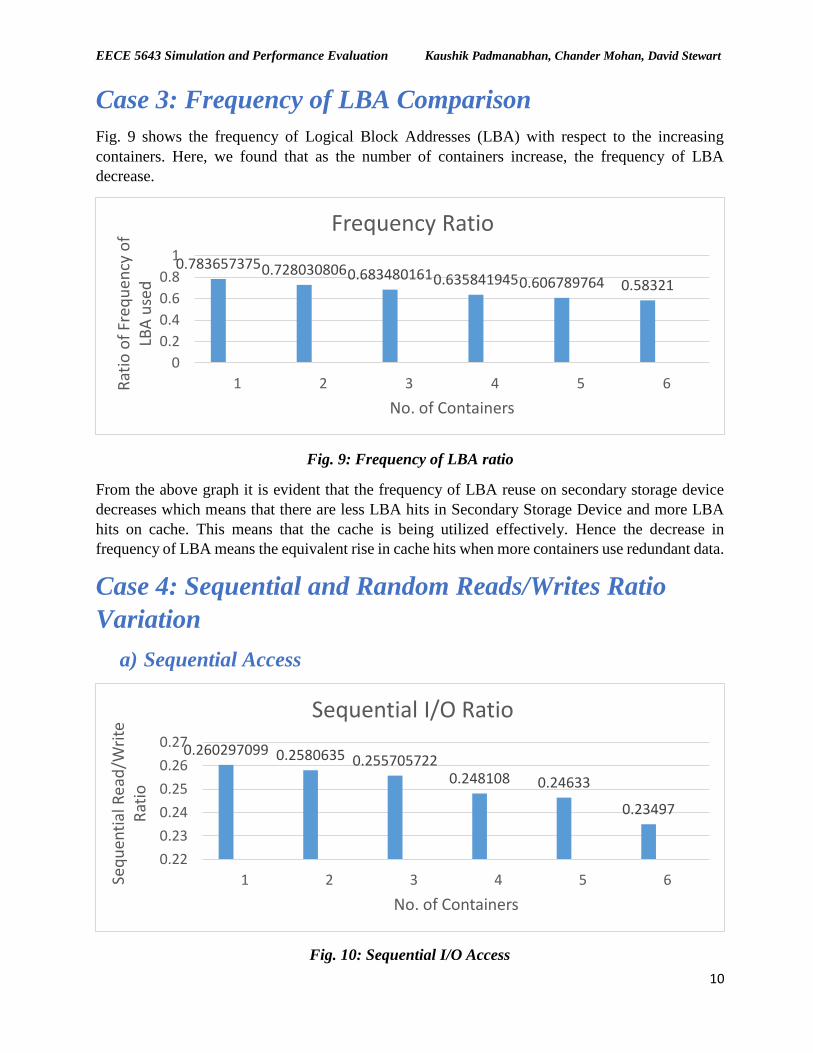
Case 3: Frequency of LBA Comparison

Fig. 9 shows the frequency of Logical Block Addresses (LBA) with respect to the increasing

containers. Here, we found that as the number of containers increase, the frequency of LBA

decrease.

Fig. 9: Frequency of LBA ratio

From the above graph it is evident that the frequency of LBA reuse on secondary storage device

decreases which means that there are less LBA hits in Secondary Storage Device and more LBA

hits on cache. This means that the cache is being utilized effectively. Hence the decrease in

frequency of LBA means the equivalent rise in cache hits when more containers use redundant data.

Case 4: Sequential and Random Reads/Writes Ratio

Variation

a) Sequential Access

Fig. 10: Sequential I/O Access

0.7836573750.7280308060.6834801610.6358419450.606789764 0.58321

0

0.2

0.4

0.6

0.8

1

1 2 3 4 5 6Rat

ioo

f Fr

equ

ency

of

LBA

use

d

No. of Containers

Frequency Ratio

0.260297099 0.2580635 0.2557057220.248108 0.24633

0.23497

0.22

0.23

0.24

0.25

0.26

0.27

1 2 3 4 5 6Seq

uen

tial

Rea

d/W

rite

R

atio

No. of Containers

Sequential I/O Ratio


11

Sequential access from the secondary devices memory storage decreases with the increase in

number of containers as seen from the blktrace charts, Fig. 10. This can be better explained with

the cache explanation. The cache employs the pre-fetch policy as frequently the data access in

devices is sequential and as a result the speed is benefitted from this anticipated data.

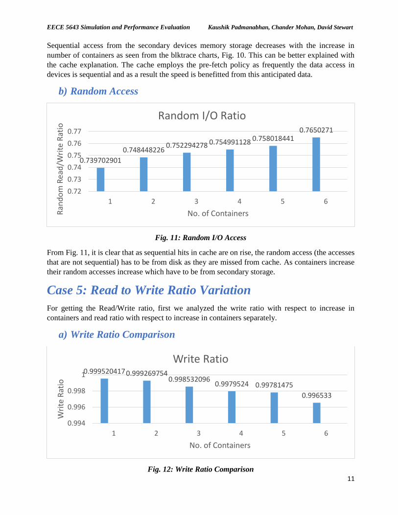
b) Random Access

Fig. 11: Random I/O Access

From Fig. 11, it is clear that as sequential hits in cache are on rise, the random access (the accesses

that are not sequential) has to be from disk as they are missed from cache. As containers increase

their random accesses increase which have to be from secondary storage.

Case 5: Read to Write Ratio Variation

For getting the Read/Write ratio, first we analyzed the write ratio with respect to increase in

containers and read ratio with respect to increase in containers separately.

a) Write Ratio Comparison

Fig. 12: Write Ratio Comparison

0.739702901

0.7484482260.752294278 0.754991128 0.758018441

0.7650271

0.72

0.73

0.74

0.75

0.76

0.77

1 2 3 4 5 6

Ran

do

m R

ead

/Wri

te R

atio

No. of Containers

Random I/O Ratio

0.9995204170.9992697540.998532096

0.9979524 0.99781475

0.996533

0.994

0.996

0.998

1

1 2 3 4 5 6

Wri

te R

atio

No. of Containers

Write Ratio


12

As the containers increase as per Fig. 12, there is an effective utilization of cache memory present

between mysql containers and hard drive when the write intensive tasks are carried out, resulting

in decrease of actual writes to secondary memory as tpcc is write intensive and writes are managed

by cache effectively.

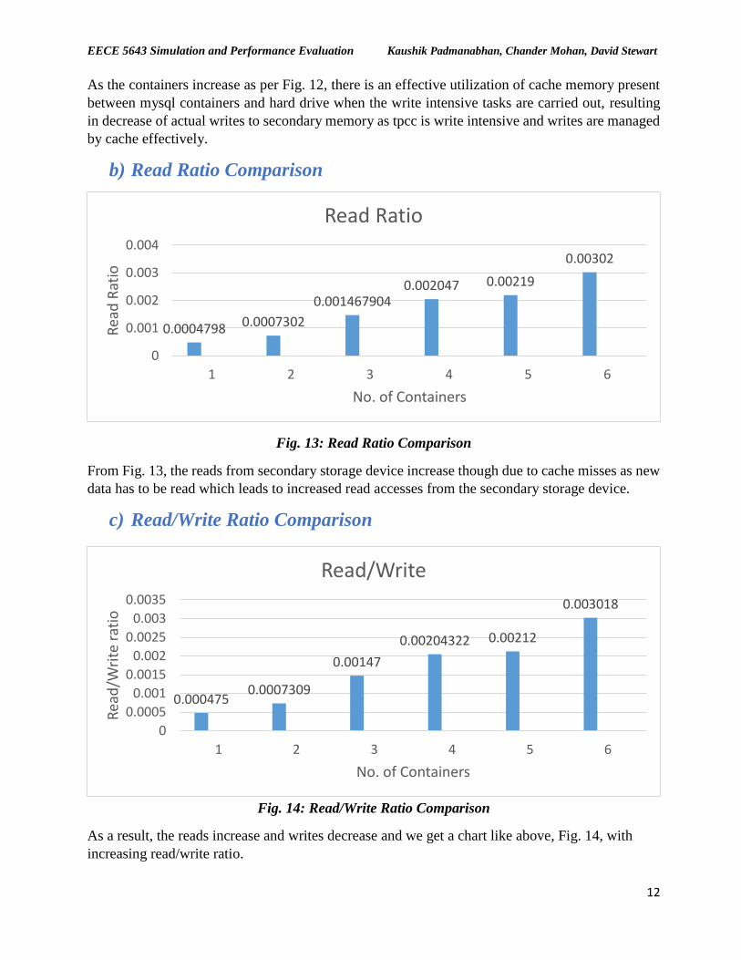
b) Read Ratio Comparison

Fig. 13: Read Ratio Comparison

From Fig. 13, the reads from secondary storage device increase though due to cache misses as new

data has to be read which leads to increased read accesses from the secondary storage device.

c) Read/Write Ratio Comparison

Fig. 14: Read/Write Ratio Comparison

As a result, the reads increase and writes decrease and we get a chart like above, Fig. 14, with

increasing read/write ratio.

0.0004798 0.0007302

0.0014679040.002047 0.00219

0.00302

0

0.001

0.002

0.003

0.004

1 2 3 4 5 6

Rea

d R

atio

No. of Containers

Read Ratio

0.0004750.0007309

0.00147

0.00204322 0.00212

0.003018

0

0.0005

0.001

0.0015

0.002

0.0025

0.003

0.0035

1 2 3 4 5 6

Rea

d/W

rite

rat

io

No. of Containers

Read/Write


13

Conclusion

The performance of containers starts degrading after 3 containers for the given system and workload

constraints. Thus, to get best performance the simultaneous running containers should be restricted

to 3 for the given specifications. Any increase results in slight degradation in performance.

The cache in the system provides an edge in system performance when containers are increased and

simultaneously the benchmark load is run in all the containers.

The performance of Docker containers is measured with increasing number of containers in terms

of different metrics and is found that different metrics are affected differently.

Future Work

Although the default system cache in the system boosts performance when containers are more. But

a cache driver designed especially for the given workload context as seen in slacker paper may

boost performance significantly especially if large number of containers with same images are run.

Project Files

Our project files (Algorithm, blktraces, iostat results, tpcc benchmark) are included in the GitHub.

GitHub: https://github.com/KaushikKPDARE/DockerPro

Acknowledgements

We wish to acknowledge each and every one who played a major or minor part which resulted in

the successful accomplishment of this project. We would especially like to thank our course

professor, Dr. Ningfang Mi and Janki Bhimani, a Ph.D. Candidate, who guided us throughout the

entire project, in each and every way possible.

Reference

a) https://docs.docker.com/engine/getstarted/

b) https://docs.docker.com/engine/installation/linux/ubuntulinux/

c) https://docs.docker.com/engine/userguide/

d) https://www.percona.com/blog/2013/07/01/tpcc-mysql-simple-usage-steps-and-how-to-

build-graphs-with-gnuplot/

https://github.com/KaushikKPDARE/DockerPro

Date post:	07-Jan-2017
Category:	Documents
Upload:	kaushik-padmanabhan
View:	81 times
Download:	0 times

Project Final Report

Documents