NASA -. sj \ NASA CONTRA REPORT CTOR PROJECT FOG DROPS Part I: Investigations of Warm Fog Properties by R. Pilie, W. Eddie, E. Muck, C. Rogers, und W, Kocmond Prepared by CORNELL AERONAUTICAL LABORATORY, INC. Buffalo, N.Y. 14221 for George C. Marshall Space Flight Center i . 1 NATIONAL AERONAUTICS AND SPACE ADMINISTRATION l WASHINGTON, D. C. . AUGUST 1972
Transcript
NASA
-. sj
\ NASA
CONTRA
REPORT
CTOR
PROJECT FOG DROPS
Part I: Investigations of Warm Fog Properties
by R. Pilie, W. Eddie, E. Muck,
C. Rogers, und W, Kocmond
Prepared by
CORNELL AERONAUTICAL LABORATORY, INC.
Buffalo, N.Y. 14221
for George C. Marshall Space Flight Center i
. 1
NATIONAL AERONAUTICS AND SPACE ADMINISTRATION l WASHINGTON, D. C. . AUGUST 1972
Part n is CR-2079, PROJECT FOG DROPS, Laboratory Investigations
6. 4ESTW4CT
A detailed study was made of the micrometeorological and microphysical characteris tics of eleven valley fogs occurring near ElmFra, New York. Observations were made of temperature, dew point, wind speed and direction, dew deposition, vertical wind velo- city, and net radiative flux. In fog, visibility was continuously recorded and peri- odic measurements were made of liquid water content and drop-size distribution. The observations were initFated in late evening and continued until the time of fog dissi- pation. The vertical distribution of temperature in the lowest 300 meters and cloud nucleus concentrations at several heights were measured from an aircraft before fog formation. The behavior of these parameters before and during fog are discussed.
A numerical model was developed to investigate the life cycle of radiation fogs. In the atmosphere, the model predicts the temporal evolution of the vertical distri- butions of temperature, water vapor, and liquid water as determined by the turbulent transfer of heat and moisture, The model includes the nocturnal cooling of the earth's surface, dew formation, fog drop sedimentation, and the absorption of infrared radia- tion by fog. The capabilities and limitations of the model are examined.
7. KEY WORDS (8. DISTRIBUTION STATEMENT
IS. SECURITY CLASSIF. (d thh rrport) 20. SECURITY CLASSIF. (Or thh c.~.e) 21. NO. OF PAGES 22. PRICE
Unclassified Unclassified 150 $3.00 --
l For sale by the National Technical Information Service, Springfield, Virginia 22151
TABLE OF CONTENTS
Section Page
LIST OF TABLES iii
LIST OF FIGURES iv
ABSTRACT
SUMMARY
ACKNOWLEDGEMENTS
I. INTRODUCTION
II. FIELD INVESTIGATIONS
Visual Observations and Visibility Data
l Surface Observations l Fog Top Altitude
Micrometeorological Data
l Low Level Temperature Data l Temperature Aloft l Summary of Temperature Data l Low Level Dew Point Data l Dew Deposition and Evaporation Rates l Wind Speed and Direction l Vertical Wind Speed and Direction l Radiation
Fog Microphysics Data
l Drop-Size Distributions l Liquid Water Content l Summary of Surface Microphysical Properties
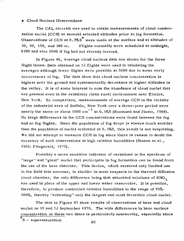
of the Fog l Drop-Size Distributions Aloft l Cloud Nucleus Observations
III. DISCUSSION OF EXPERIMENTAL RESULTS
l Fog Formation Processes at Elmira l The Role of Dew in the Fog Life Cycle l Evolution of Drop-Size Distributions and
Associated Implications
IV. NUMERICAL MODELING OF RADIATION FOG
Introduction
l Brief Description of Model l Previous Work
i
vii
viii
xi
1
3
7
7 15
16
16 29 35 40 49 50 55 59
- 60
!“5-
70 76 80
84
84 91
94
99
99
99 100
Section
Numerical Model 102
l Major Assumptions o Equations
List of Symbols Maj’or Equations Saturation Adjustment Radiation Exchange Coefficients Terminal Velocity of Fog Drops
l Boundary Conditions Upper and Lower Boundaries The Surface
l Computational Procedure Grid System Implicit Integration Summary of Computational Sequence Timing
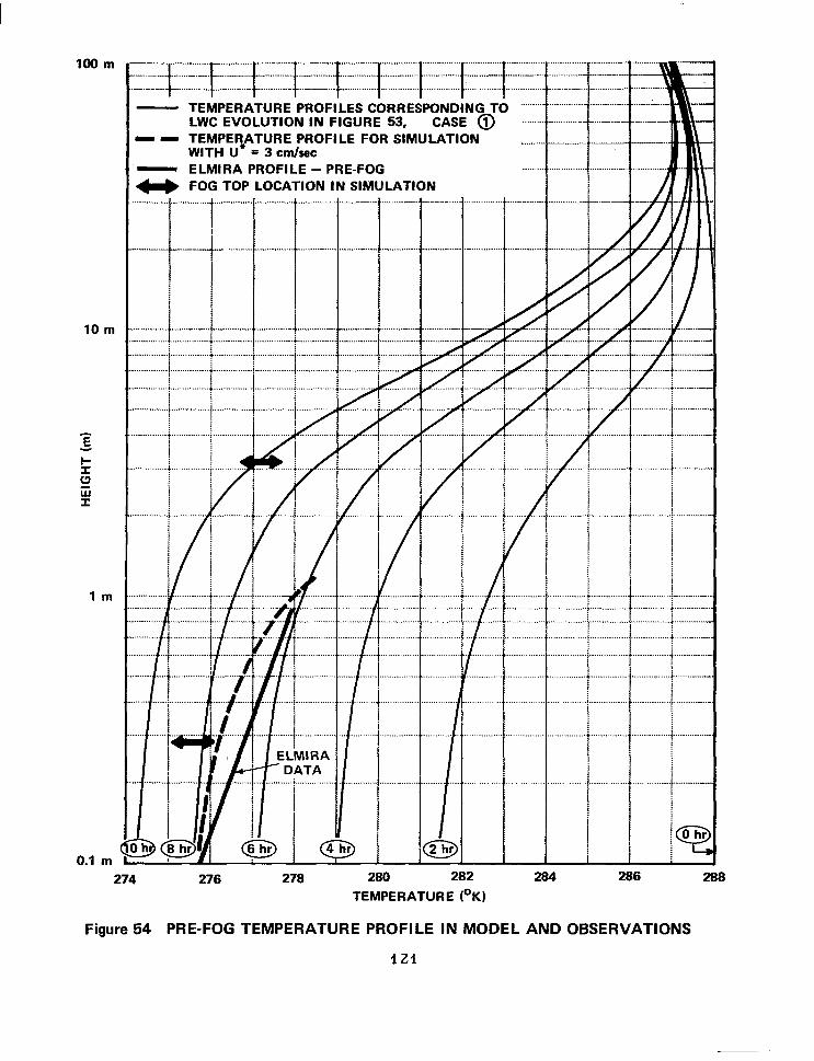
* General Characteristics of Model Fogs l Example of Model Fog Formation
Temperature Structure Prior to Fog Formation Temperature Structure After Fog Formation
l Exchange Coefficient as a Function of Thermal Stratification
# Model Behavior as a Function of Input Parameters l t Dew Formation 0 Summary
128 130 131 132
REFERENCES 135
Page
I
-
ii
LIST OF TABLES
Table No. Page
I
11
III
Instrumentation
Extremes of Deviation of Observed Temperature Relative to Average Temperature
Growth of Droplets at 0.3$@ on Nuclei of Different Activation Supersaturationa
4
24
97
IV
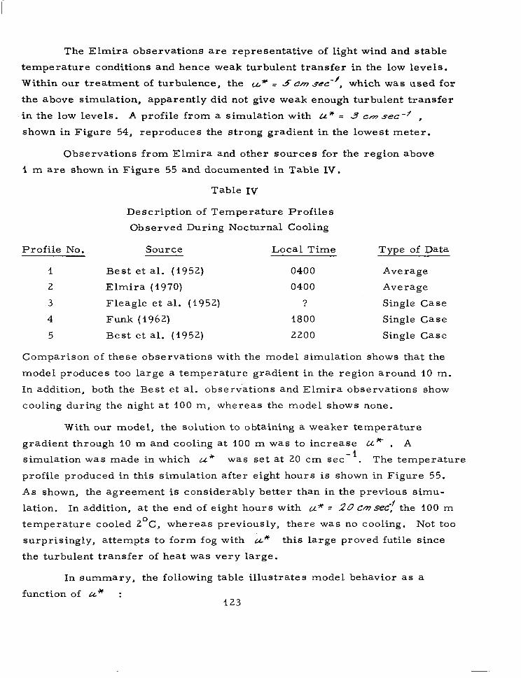
V
Description of Temperature Profiles Observed During Nocturnal Cooling
Model Behavior as a Function of u*
123
125
VI Stratification of Numerical Experiments by K -Value at the i0 m Level 130
iii
LIST OF FIGURES
Figure No.
1
2
10
11
12
13
14
15
16
17
18
19
Topography Near the Elmira Field Site
Schematic of Chemung County Airpo,rt Showing Instrumentation Sites
Visibility vs Time 8/22/70
Visibility vs Time 9/12/70
Visibility vs Time 9/2/70
Visibility vs Time 8/13/70
Visibility vs Time 8/ 26 J70
Fog Top Altitude as a Function of Time
Average Fog Top Altitude as a Function of Time After Formation
Temperatures and Dew as Functions of Time 8/22/70
Tempe?‘amres and Dew as .Functions of Time 9 Ji2 J70
Temperatures and Dew as Functions of Time 9/2/70
Model Fog Temperatures - Surface to 17 m
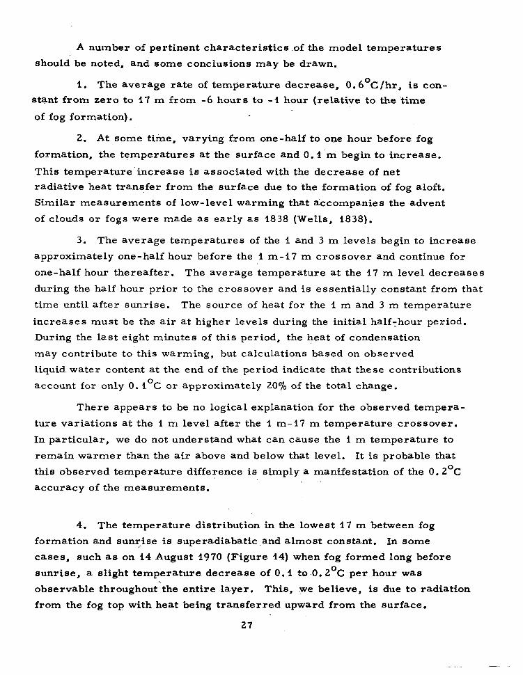
Temperature as a Function of Time 8 J 14 J70
Temperature Aloft 8/22/70 and q/2/70
Temperature Aloft 8/13/70
Summary of Temperatures at 30 and 60 m as a Function of Time (8 fogs) (C0rrecte.d for Sunrise Effect)
Summary of Temperatures at 90 and 120 m as a Function of Time (8 fogs) (Corrected for Sunrise Effect)
Vertical Distribution of Temperature Relative to Temperature of Fog Top
Page
5
6
9
10
11
12
13
17
18
20
21
22
25
28
31
32
33
34
36
iv
Figure No.
20
21
22
23
24
25
26
27
28
29
30
31
32
33
34
35
36
37
38
39
40
Model Temperature Profiles - Pre-Fog and Fog Formation Periods
Model Temperature Profiles in Fog, 38
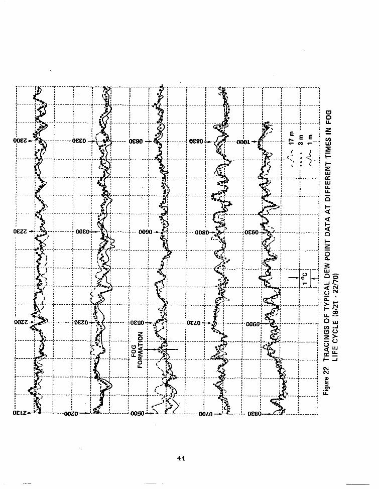
Tracings of Typical Dew Point Data at Different Times in Fog Life Cycle (8/21-8/22/70) 1,
Dew Points as Functions of Time 8 J22 J70
Dew Points as Functions of Time 9 J 12 J70
Dew Points as Functions of Time 9 J 2/70
Dew Point Model
Dew Point as Function of Time 8/14/70
Dew Formation-Evaporation Model- -Spread in Data Points is Shown
Wind Data 8 J22 J70
Wind Data 9 /2 J70
Vertical Wind Speed as Function of Time (9/11-12/70)
General Envelope.of Peaks in Vertical Wind Speed (Isolated Peaks Neglected) 9 J 12 J 70
, Drop-Size Distributions Obtained on 2 Sept 1970
Drop-Size Distributions Obtained on 8/ 25 J 70
Drop-Size Distributions Obtained on 8 J 22 J 70
Drop-Size Distributions Obtained on 9 J 12 J 70
Comparison of Liquid W,ater Content,Measurements Made with a Gelman High Volume Sampler and Simul- taneous Values Obtained by Integrating the Absolute Drop-Size Distribution / \
Visibility and Microphysics Data.0btaine.d on 8/22 J70
Visibility and Microphysics Data Obtained on 9 /I2 J70
Visibility and Microphysics Data Obtained on 9/2/70
Page
37
41
43
44
45
47
48
51
53
54
56-57
58
64
66
67
68
69
71
72
73
V
Page
74
75
Figure No.
41
42
43
Visibility and Microphysics Data for Seven Fogs
Mean Drop Sizes as Functions of Time for Seven Fogs
Normalized Drop-Size Distributions Obtained Aloft on 8/22/70 77
44 Normalized Drop-Size Distributions Obtained Aloft on 9/12/70 78
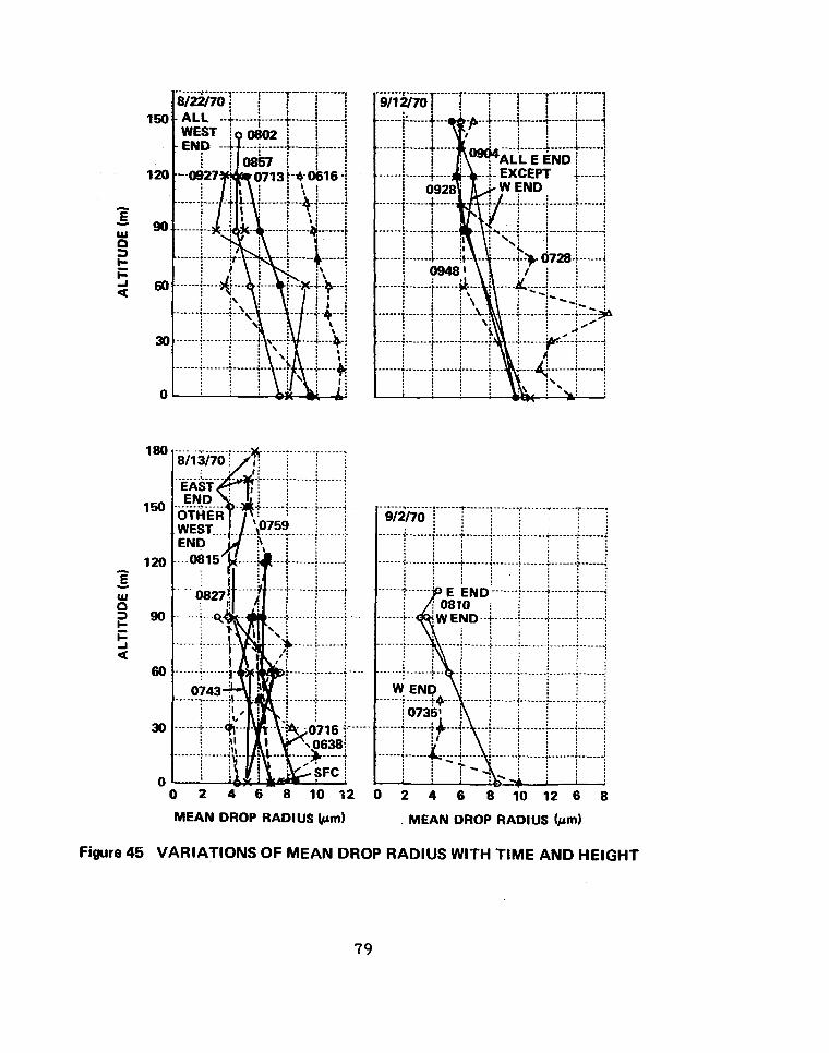
79 45
46
Variations of Mean Drop Radius with Time and Height
Vertical Profiles of Cloud Nucleus Concentration at Three Times - Average Data from 12 Flights at S = 0.37” 81
82
86
87
47
48
49
50
Haze Nuclei Data
Nocturnal Cross Valley Circulation (After Wagner)
The Nocturnal Mountain Wind
Calculated Dew Point Change between t = -6 Hours and t= -0.5 Hour Required to Produce Measured Dew Deposition in Same Time Interval 92
51 Model Fog Top Heights vs Time. Numbering Labels Particular Numerical Experiment for Which Data are also Shown in Figure 52 117
119 52 Model Fog Liquid Water Content vs Time
53 Example of Model Time-$Ieight Variation of Liquid Water Content (in mg/m )- Case (1) in Figures 51 and 52 120
121 54
55
Pre-Fog Temperature Profile in Model and Observations
Comparison of Model Temperature Profiles to Observed Profiles for Pre-Fog Conditions 124
Model Low-Level Temperature Profile Evolution in Fog After Surface Net Radiation Becomes Negligible
56
57
127
Evolution of Turbulent Exchange Coefficient Profile for Model Simulation in Which Low-Level Temperature Profile Becomes Lapsed 129
vi
SUMMARY
Extensive measurements were made of micrometeorological and
microphysical characteristics of eleven fogs in the Chemung River Valley
near Elmira, New York. Temperature was measured at five levels between
0 and 17 m, dew point at three levels, and wind speed and direction at two
levels. Net radiative flux and vertical wind velocity were measured at 17 m.
Visibility was observed at three locations at a height of four feet, and dew
deposition was measured at the surface. Observations began in late evening
and continued until the time of fog dissipation. After fog formed, drop
samples were collected.for size distribution analysis and liquid water content
was measured at 15-minute intervals or less. The vertical distribution of
temperature from 0 to 300 m and cloud nucleus concentrations were measured
from an aircraft at three-hour intervals before fog formation. Temperature
measurements and drop sample collections were made in fog at altitudes
above 60 m.
Remarkably consistent patterns of temperature, dew point, and dew
deposition behavior with time relative to fog formation were observed from
six hours before fog formed to fog dissipation. Radiative cooling of the
surface stimulated dew deposition and formation of temperature and dew
point inversions. After midnight, maximum cooling occurred at a level equal
to about two-thirds the eventual fog depth, apparently as a result of nocturnal
valley circulations. When the low level atmosphere became about isothermal,
fog formed aloft and’grew downward under the influence of an instability caused
by radia’tion from the fog top. Surface warming began when net radiation from
the surface was reduced by fog aloft. When fog was fully developed, the
temperature profile was approximately wet adiabatic in the lowest two-thirds
of the fog and inverted at higher levels. After sunrise, fog temperature
increased uniformly.
Dew deposition rate was uniform before fog formation and decreased
to near zero between fog formation and sunrise. Evaporation of dew began
at sunrise and continued until fog dissipation. The evaporation rate was
sufficient to maintain saturation for approximately 2.5 hours within the fog
as post sunrise temperatures increased. AS the heating rate increased,
evaporation was insuffxcient and the fog lifted.
vii
As long as ambient wind speeds were low, the mountain wind controlled
flow in the valley. Directional shear of 45-90° occurred frequently and
150 to 180° shear was occasionally observed between valley and hilltop winds.
Bursts of vertical air motions, both up and down, occurred throughout the
pre-fog period. Occasionally, persistent up- or downdrafts occurred for
intervals of several minutes-. Up and down motions of ‘short duration occurred
continuously after fog formation with typical velocities of 0. 5 to 1 m set -1
and occasionally as large as 2 m set -1 .
The microphysical properties of fog change in a manner that is almost
as consistent as the micrometeorological properties. Shallow ground fog
usually occurs prior to the formation of deep valley fog. The ground fog
consists of 100 to 200 droplets cm -3 distributed between 1 and 8 pm radius,
with a mode at 3 to 4 pm. As deep fog begins to form, the drop concentration
decreases to less than 5 cm -3 and the mode increases to 6 to 10 pm radius.
Droplets smaller than 3 to 4 pm radius disappear completely. Total droplet
concentration then increases slowly to a maximum at the first visibility
minimum at which time small droplets reappear. Thereafter, the distribution
contains droplets between 1 and 30 pm radius with a mode between 6 and
12 pm. In about half of the fogs, a second mode, at 3 or 4 pm also exists. It
appears that the initial visibility degradation at the surface occurs as a result
of droplets being physically transported downward from the fog aloft and that
new droplets are not generated in the very low levels until the first visibility
minimum.
A numerical model was developed to investigate the life cycle of fogs
which result both from the nocturnal cooling of the earth’s surface by infrared
radiation and from various vertical transfer processes. In the model, the
atmospheric exchange coefficients are functions of friction velocity, height,
and the predicted local thermal stability. After the earth’s surface is cooled to
the dew point, dew is allowed to form and water vapor is brought down to the
surface by turbulent transfer. Upon fog formation, the influences of infrared
absorption and radiation by fog, and fog drop sedimentation are included. The
model has a one-dimensional vertical grid system which extends from one
meter below the earth’s surface to approximately one kilometer above the
viii
surface. In the atmosphere, the model predicts the temporal evolution of the
vertical distributions of temperature, water vapor, and liquid water as deter-
mined by radiative and turbulent transfer of heat, and turbulent transfer of
moisture.
Because the temperature and dew point profiles decreased simultaneously
during a simulation, the model behavior was quite sensitive to the overall level
of turbulent transfer as controlled by the friction velocity. The mode 1 formed
radiation fog with tops in the 10-40 m range but could not duplicate all the
observed characteristics of the Elmira valley fog in a single simulation.
This result suggests that two- or three-dimensional processes, e. g., valley
circulations, may significantly influence the formation and properties of the
Elmira valley fogs. The liquid water content of the deeper fogs generated was
in the 300-500 mg/m3 range, 3 which is larger than the 150 mg/m frequently
observed in natural fogs. This discrepancy between observations and model
results appears to lie in the inability of the model to predict deep fogs with
realistic initial dew point spreads. The present model was able to reproduce
a characteristic feature which occurs after fog forms, i.e., a rise of surface
temperature and conversion of the low level temperature profile from inversion
to lapse conditions. In the model, this behavior occurred when downward radi-
ation emanating from the fog significantly reduced the net radiation from the
earth’s surface.
ix
ACKNOWLEDGEMENTS
The authors wish to express their gratitude to members of the
Atmospheric Sciences Section and Environmental Systems Department who
participated in this program and who contributed many extra hours of their
time during the performance of this project. In particular, special thanks
are due Mr. George A. Zigrossi for his assistance in data taking and for his
skillful maintenance of instrumentation and to Miss Christine R. Schurkus
for typing this manuscript and for participating in the tedious reduction of
drop-size data.
Thanks are due Mr. Ed Wronkowski, Airport Manager of the
Chemung County Airport, Elmira, New York for allowing us to use the
many airport facilities and services. We also wish to thank members of the
Elmira ground control, headed by Mr. Jim Mengus, Chief Air Traffic
Controller. Mr. William Garrecht, Chief of the Airways Facilities Section
of the FAA was particularly helpful in arranging needed clearances for
operating equipment in restricted areas of the airport.
We are indebted to Dr. Peter Kuhn, of the National Oceanic and
Atmospheric Administration, for providing US with net radiometers and
for assisting in the interpretation of the results.
Finally, our sincere appreciation is given to Mr. William A. McGowan,
Chief, Aircraft and Airport Operating Problems Branch at NASA Headquarters,
who has served as our project monitor for the past eight years and who has
given us his continued encouragement and support throughout the performance
of this project.
X
CHAPTER I
INTRODUCTION
During the summers of 1968 and 1969, Co.rnell Aeronautical Laboratory, Inc.
AL), under the sponsorship of the Aeronautical Vehicle Division of NASA,
erformed extensive valley fog seeding tests near Elmira, New York.
The seeding concept developed at CAL is one in which visibility is improved
by introduc.ing sized hygroscopic materials into the fog. The nuclei, upon
entering the fog, cause a favorable redistribution of dr.oplet size which
often results in substantial visibility improvements. In approximately half
‘of the airborne seeding experiments that were performed some visibility
tmprovement was -measured. These successful experiments were concen-
2rated in the second half of the fog life cycle. Experiments performed
shortly after fog formation were not successful. Similar relationships
yere observed in experiments performed by the Air Force ,Cambridge
esearch Laboratory and Meteorology Research, Inc., in Lakeport and
he Noyo River Valley, California.
n the character of fog that might be responsible for the observed differences
/
A review of the literature provided no explanation for the changes
seeding effectiveness . It was apparent that our lack of understanding of
he temporal variations of the physical and dynamic characteristics of fog
as beginning to limit progress in the development of fog dissipation
rocedures. To provide some of the needed information, therefore, the
970 field program was designed to gather information on the entire fog
life cycle. The field program was to be followed by an effort to formulate
a dynamic model of valley fog. The goal was to set initial boundary con-
$ itions and input parameters in the computer model according to measure-
ments obtained in the field and let the computer reproduce the variations
J ‘n fog characteristics that were observed through the natural life cycle.
In addition to these investigations of the properties of natural fog,
series of laboratory experiments were performed to complete the investi-
of the possibility of inhibiting fog formation through the use of
inhibitors and to begin to study the effects of some common
pollutants on the characteristics of fog and on the seedability of fog.
ests were also initiated to examine the photochemical production of
These experiments were conducted in anticipation of
i
our current study of coastai fogs at Vandenberg, California and in the
Los Angeles Basin. Results of the laboratory tests are presented under
separate cover.
Chapters II and III in this report cover the results of the field pro-
gram. Results obtained from the numerical modeling effort are presented
in Chapter IV.
CHAPTER II
FIELD INVESTIGATIONS
Field investigations were performed at the Chemung County Airport
near Elmira, New York from 5 August through 15 September 1970. The
general characteristics of the valley are illustrated in Figure 1, and
locations of our instrumentation on the airport are shown in Figure 2.
Transmissometers were located at the localizer, the tower site, and the
glide slope. All other instrumentation listed in Table I was located at the
tower site or on the Piper Aztec used for airborne observations.
Automatic instrumentation was usually turned on between 2100
and 0100 on the nights preceding the predicted fog formation. Manual
observations were usually made at half-hour intervals from that time
until fog dissipation and occa’sionally at much shorter intervals (as
small as 30 seconds) when a particular characteristic of the atmosphere was
being investigated in detail. Normally, aircraft observations were made at
three-hour intervals from midnight until fog formation. After fog forma-
tion, regular aircraft observations were suspended for safety reasons
until after daybreak. Shortly after sunrise, aircraft data were acquired
from the surface to several thousand feet on takeoff through the fog and at
approximately 45-minute intervals thereafter on ILS approaches to 60 m.
Measurements were made on 19 occasions when the probability of
fog formation was estimated to be 50% or greater. Fog formed on 12 of
these occasions and on two days for which the probability had been estimated
at less than 50%. On five of the seven nights for which fog was forecast
(probability > 50%) but did not form, thin clouds drifted over the valley and
inhibited surface cooling. On the other two nights, fog formed in other
parts of the valley but not at the airport.
The data presented in this report are based on eleven of the twelve
fogs sampled, Calibration of all equipment was not completed until
12 August 1970 so that only portions of the data pertaining to the fogs of
8 and 11 August are included in the summaries.
3
SURFACE
THREE TRANSMISSOMETERS (CAL)
DROP SAMPLER (CAL-GELATIN)
LIQUID WATER CONTENT (GELMAN)
DROP CONCENTRATION (CAL) l
TEMPERATURE (SURFACE AND. IO cm)
DEW WEIGHT (CAL)
HAZE NUCLEI (CAL)
TOWER
TEMPERATURE - 1 m, 3 m, 17 m DEW POINT - 1 m, 3 m, 17 m WIND SPEED & DIRECTION, 3 m, 17 m
VERTICAL WIND SPEED, 17 m NET RADIATION, ?7 m
AZTEC
CLOUD CONDENSATION NUCLEI (CAL)
TEMPERATURE (REVERSE FLOW)
DEW POINT (CAMB. INST.) DROP’SAMPLER (CAL)
Table I
INSTRUMENTATION
(FOXBORO)
(FOXBORO) (BEC & WHIT)
(GILL) (APCL)
RECORDING INTERVAL -
CONTINOUS
15 MIN
30 MIN 15 MIN
30 MIN
30 MIN
3 HR
CONTINUOUS CONTINUOUS
CONTINUOUS
CoNTlNUOUS 30 MIN
3 HR CONTINUOUS
CONTINUOUS 100 FT VERT. --.
T I
DATA QUALITY
GOOD
X
X
X
XI
X
X X
X
X
X
FAIR
X
X
X
X
POOR
X
X
-.?- -_
*TWO METHODS WERE USED.
4
Figure 1 TOPOGRAPHY NEAR THE ELMIRA FIELD SITE
JJ
-Fig
ure
2 SC
HEM
ATIC
O
F C
HEM
UN
G
CO
UN
TY
AIR
POR
T SH
OW
ING
IN
STR
UM
ENTA
TIO
N
SITE
S
Of the twelve fogs for which data were acquired, eight formed
within the two hours preceding sunrise, three formed within the half hour
after s&rise and one (14 August 1970) formed at 0015 EDT, an anomaly
caused by the saturation of the valley air after an early evening thunderstorm.
In the presentation of the data throughout this report, the two fogs of
22 August and 12 September are used as examples of typical persistent,
dense fogs that form prior to sunrise. Data from 2 September 1970 are
used to illustrate characteristics of fogs that form after sunrise. Other
examples are sometimes presented to illustrate specific features of a given
fog that do not fit the general patterns.
It should be recognized that all data were acquired,in one valley and
that attempts should be made to verify the findings at other locations.
VISUAL OBSERVATIONS AND VISIBILITY DATA
l Surface Observations
_ Visibility data were acquired from CAL-designed transmissometers
located at three sites on the airport as indicated in Figure 2. The trans-
missometers were operated over 100 ft path lengths at a height of 4 ft above
the surface. Each instrument was adjusted in situ to provide a measured
transmitter beam width of less than 1’ . Receiver beam width was
adjusted in the laboratory to be less than 1 o . Maximum overall error in the measurement of received light intensity was estimated to be *50/o,
with the greatest limitation being imposed by the accuracy of the recorder
(*I% full scale) at the lowest visibilities. This error is negligible in the
low visibility region; e. g., at 1000 ft visibility, an error of *50/o in the
measurement of received light produces an error of only k100 ft in
visibility. To minimize error due to drift in the transmissometers, a
calibrate-signal was generated with a prism inserted into the transmitted
beam to reflect a fixed fraction of the transmitted light into a second photo-
tube mounted in the transmitter. The calibrate-phototube was operated
from the same power supply as the receiver and its output was passed
through the receiver electronics. Calibrate+ignals were, recorded for
20-second intervals every three minutes.
7
Continuously recorded transmissometer data were converted to
meteorological visibility V in the standard manner. That is,
I = IOeBpX (1)
v = 3.912 P
(2)
where I and I are observed light intensities at the receiver after trans- 0 mission through the turbid and clear media respectively, x is the trans-
mission path length (100 ft in this case) and p is the extinction coefficient.
Conversions were made at discrete times determined by changes in trans-
mission characteristics or to coincide with the acquisition of drop samples.
Visibility data acquired during the three fogs used for illustrative
purposes throughout this report (22 August,and 2 and 12 September 1970) are
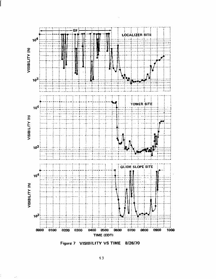
shown in Figures 3, 4, and 5, The data in Figures 3 and 4 are characteristic
of persistent, dense fogs in Elmira and the data in Figure 5 are typical of
fogs that formed shortly after sunrise. ,Figure 6, which shows data acquired
on 13 August 1970, illustrates typical visibility fluctuations associated with
patchy fog. Figure 7 illustrates the one case (26 August 1970) in which fog
was persistent at two of the instrumented sites and patchy at the third.
Several features of the illustrative curves require explanation.
The continuous curves show meteorological visibility obtained from trans-
missometer data. The x’s show visual range as determined by an observer
either by pacing off the appropriate distance or measuring it. with an
automobile odometer . The disagreement after daybreak is due to airlight
and illustrates why daytime and nighttime scales are different on RVR
equipment .
With the 100 ft baseline, the least count of the transmissometers was
such that visibility in excess of about ,13,000 ft was not distinguishable from
infinity. The dashed portions of the curves simply indicate that visibility
exceeded that value. Visual observations made during this period indicate
that haze usually formed in late evening and limited visibility to about three
.._ NOTE: DATA POINTS INDICATED BY ! DATE OF OBSERVATION
j
-4 ; : ;
TIME RELATIVE TO 1 - 17 m TEMPERATURE CROSSOVER (hr)
(b) MODEL FOG TEMPERATURE - 50 m LEVEL
Figure 17 SUMMARY OF TEMPERATURES AT 30 AND 60 m AS A FUNCTION OF TIME (8 FOGS) (CORRECTED FOR SUNRISE EFFECT)
33
. .-
DATES CIRCLED
TIME RELATIVE TO I’- 17 m TEMPERATURE CROSSOVER (hr)
(a) MODEL FOG TEMPERATURE - 60 m LEVEL
: : : : SUN% i ! , .
. . : i _ ;.. . .
+2 +3
:
:
i : .
+4 ‘.
TIME RELATIVE TO 1 - 17 m TEMPERATURE CROSSOVER (hr)
(b) MODEL FOG TEMPERATURE - 120 m LEVEL
Figure 18 SUMMARY OF TEMPERATURES AT 90 AND 120 m AS A FUNCTION OF TIME (8 FOGS) (CORRECTED FOR SUNRISE EFFECT)
34
It is apparent from Figure i7- that the consistent temperature behavior
noted in the low-leveLdata persists to at least the 60 m altitude. No data ^. point differs from the best mean fit by mor,e than 1. 5OC. Substantially
greater spreads are evident in the data for 90 and 120 m shown in Figure 18.
l%ere, the data are split into two groups, with normalized temperatures
for 11, 13,: and 22 August averaging more than a degree colder than those
of other dates ; Examination of other data shows that the temperature group-
ing is consistent with a grouping of the data in accordance with fog height.
With the exception of a single observation in one fog, the maximum height . of the fog on each of the circled dates in Figure 18, representing the warmer
group, was less than 120 m while the maximum height of the fog on each of
the uncircled dates, the colder group, exceed 150 m. Apparently, the
maximum pre-fog cooling rate occurs at a level which is slightly below
(about one-third of the eventual fog’ depth) the eventual fog top, and from
the convergence of the data, the atmosphere beneath that level is very
nearly isothermal at the time of fog formation.
Attempts to perform this kind of analysis for altitudes above 150 m
were fruitless because of the wide scatter in the data. In the belief that this
scatter may be associated with the wide distribution of height of the fog top,
we examined the temperature distribution about the fog top. Results are
presented in Figure 19. It is apparent that the distributions are all reversed
“S” shaped with the point of inflection within 15 m of the fog top. For a
given fog, the steepness of the inversion remains approximately constant with
time, but there is significant variability from fog to fog. The average strength
of the inversion at fog top is approximately 2. 5OC per 100 m.
l Summary of Temperature Data
The results of these various analyses of temperature distribution
with time are summarized in the family of temperature profiles presented
in Figures 20 and 21. The curves shown in Figure 20 were obtained by
replotting points taken from the curves in Figures 11, 27, and 18. In
Figure 21, the data for lower levels were obtained from Figures 11, 17,
and 18, and the data for upper levels were obtained by averaging the data at
each height in Figure 19 and faired into the lower curves.
35
L
; .-----mm i -_-mm- + -e---e $ m-e--_-
I :
:-------:-------*-------+-----------------~------~ I
, I
1 I I I
I
! I
:
I
: :
: : :
I I
I I I
, I I I
i 1 : , I +90~------:-------t-------:-------~-------~---
I IO i ~&~~~; ------- j --__--- /
- Y +a I------1
“I LL 8125
I I 1 I 8 I 6126
8 I i 6
: : I
I I I I I
I. I I I
I I I +a ;------i------:‘------;t-----:--;------- _-___- _-____; -
I 1 :
I I
: -----(.
I i I i
t
I
i
I
: , I 6 L , I I
I I
: i i :
: :
:
---:----*t-------i-------: I I I
: i
6 I 4
!
-4 -3 -2 -1 0 +1 +2 +3 +4
TEMPERATURE RELATIVETOTEMPERATUREOF FOGTOP
Figure 19 VERTICAL DISTRIBUTION OF TEMPERATURE RELATIVE TO TEMPERATURE OF FOG TOP
36
,&;
! ,i
i i
& ---
---j--
-.---~
------
-r---.
------
------
0: --
-_ Q
$ -4
-3
-2
-1
0 +1
+2
+3
t4
+5
+6
TEM
PER
ATU
RE
REL
ATIV
E To
l-1
7 III
CR
OSS
OVE
R T
EMtiE
RAT
UR
E
Figu
re
20 M
OD
EL T
EMPE
RAT
UR
E PR
OFI
LES
- PR
E-FO
P AN
D F
OG
FO
FjM
ATlO
N
PER
lbD
S
180
---.-:------+------i--- \ASSUi
-1 0 +1- +2 +3 +4 +5 -1 o +I +2 +3
TEMPERATURE RELATIVE TO 1-17 m CROSSOVER TEMPERATURE
Figure 21 MODEL TEMPERATURE PROFILES IN FOG
Average curve from Figure 19 adjusted in height to correspond to three possible fog top heights (arrows) and faired into curves obtained from Figures 13, 18 and 19.
38
The important information evident from this presentation is as follows:
I. The intensity of the pre-fog inversion gradually decreases between
30 and 9b m altitudes during the last six hours before fog formation. At
lower levels, the inversion intensity remains about constant until approxi-
mately one-half hour before fog formation. I
2. During the last half hour before fog, the low-level inversion
breaks. At the time of fog formation, the atmosphere is approximately
isothermal in the lowest two-thirds of the fog depth. The temperature is
inverted at higher levels.
3. Within 15 minutes after fog formation, temperature distribution
in the lowest 17 m becomes superadiabatic; and above that level, it is
approximately wet adiabatic through the lowest two-thirds of the fog depth.
An inversion, with maximum intensity slightly above the fog top, exists
at higher levels. This condition persists without significant change until
sunrise. Surface warming after sunrise causes the temperature lapse to
increase at Low levels until fog dissipation. Similar observations of the
existence of a near wet adiabatic lapse rate in fog have been reported by
Fleagle et al. (1952) and Heywood (1931).
4. The rate of temperature increase of the fog after sunrise increases
from 0.2OC/hr in the first hour, to 0.7 and 1.2OC/hr in the second and
third hours, respectively.
Other pertinent conclusions which are more evident in earlier
presentations are:
1. The surface and low-level temperatures decrease at a constant
average rate of 0.6OC/hr until one hour before fog formation. Between
one,-half and one hour before fog, the surface temperature begins to increase
rapidly. Shortly thereafter, warming begins in the lowest 3 m of atmos-
phere but cooling persists at higher altitudes until the atmosphere in the
center-valley region fs isothermal.
2. Between the time of fog formation and sunrise, the temperatures
at the surface and all levels of the fog remain constant or decrease at the
with tiine. Low-level temperatures follow with time lags that increase with
altitude.. Abovs 17 m, the ~temperature of the entire fog increases at the
same rate.
4. A substantial horizontal temperature gradient exists between the
center-valley region and the adjacent hills at the same level.
l Low Level Dew Point Data
Dew points were measured at the 4 m, 3 m, and 17 m levels and
the data recorded continuously using a Foxboro dew point measuring system. 9
Before entering discussions of the data validity, it is necessary to illustrate
certain characteristics of the records that are typical for different times
in the fog life cycle. These illustrations are presented in Figure 22.
A consistent pattern of short-period (Z- to IO-minute) fluctuations
in indicated dew point that is characteristic of all outdoor records is evident
in the samples shown in Figure 22. The fact that many of the indicated
fluctuations are correlated on the three separate instruments indicates that
in many cases at least the fluctuations are real. It is apparent, however,
that in order to obtain representative values for a given time interval, some
form of averaging is required. For ease in data reduction, we elected to do
the averaging over 7. 5-minute intervals by eye. With the care taken in the
data reduction, we believe that data point& presented in subsequent figures
represent the true average of recorded data to 310.25~C.
When the three dew cells are operated simultaneously in our 600 m3
experimental chamber, the records show none of the fluctuations that are
characteristic of the field environment. By altering the amount of ventilation
to the dew cells with a 48-inch fan, short-term fluctuations amounting to
approximately l/Z°C can be induced. The three dew cells always agree to
within 0. 25OC when operated sinl. ,aneously in the chamber. In a relative
sense, therefore, the data presented are quite accurate.
Model 270+ RG Dynalog Qewcel Element and associated electronics with ERB 6 Multipoint Recorder.
40
Figu
re 2
2 TR
ACIN
GS
OF
TYPI
CAL
D
EW P
OIN
T D
ATA
AT D
IFFE
REN
T TI
MES
IN
FO
G
LIFE
CYC
LE
(8/2
1 -
22/7
0)
The Foxboro system was factory calibrated about a year before going
into the field. Attempts to obtain absolute calibrations in the field using wet
and dry bulb thermometers usually resulted in agreement to within the
recorded dew point fluctuations that were occurring at the time. Because
of these fluctuations, and because of the inherent insensitivity of the wet
and dry bulb method at very high humidities, we suspect that the Foxboro
system provided the best measurement of humidity available to us in the
field. Perhaps the best indication of the absolute accuracy of this system
rests in the observation that the mean difference between indicated
temperature and indicated dew point at the time of fog formation was
0.3OC for the eleven cases available. The maximum indicated difference
was 1. O°C and in all other cases the difference was less than 0.6OC.
Purely on the basis of internal consistency of the data, it appears that the
dew points are accurate to -LO. 5OC in an absolute sense and probably better
in a relative sense.
Typical dew point data reduced in the manner described above are
presented in Figures 23, 24, and 25, which correspond to the temperature
data presented in Figures 10, 11, and 12, respectively. From these data
sets, it is apparent that there is a gradual decrease in dew point at low
levels in the first few hours after sunset, but no consistent change of dew
point with height is evident until near midnight. At about midnight, a rather
consistent dew point inversion forms and, with the exception of short-term
fluctuations that appear- to be associated with short-term wind fluctuations
and surface temperature increases, gradually increases in intensity until
approximately one-half hour before fog formation. At that time, probably
because of the sharp increase in surface temperature, the dew points at the
1 m and 3 m levels begin to increase rapidly.
As with the temperature inversion, the breakdown of the’dew point
inversion is complete at the time of the first visibility minimum. From that
time until sunrise, the dew point fluctuates about a constant value and
thereafter, until fog dissipation, the dew point increases gradually. As
evident in Figure 22, the period and magnitude of short-term fluctuations
42
rp
W
iloo
2200
23
00
0000
01
00
0200
03
00
0400
05
00
0600
07
00
0800
, o9
00
TIM
E (E
DT)
Figu
re 2
3 D
EW P
OIN
TS A
S FU
NC
TIO
NS
OF
TIM
E 8/
22/7
0
woo
06
00
0700
08
00
09w
TI
ME
(ED
T)
-figu
re 2
4 D
EW P
OIN
TS A
S FU
NC
TIO
NS
OF
TIM
E g/
12/7
0
coo
23liiI
W
OO
01
00
0200
03
00
0400
05
00
0600
07
00
OSW
09
00
1000
TI
ME
(ED
T)
Figu
re 2
5 D
EW P
OIN
TS A
S FU
NC
TIO
NS
OF
TIM
E g/
2/70
decrease significantly immediately after fog formation. With the gradual
increase in dew point that follows, these fluctuations also increase and
achieve maximum magnitude at about the time fog dissipates.
This typical behavior is summarized in the dew point model presented
in Figure 26, which was constructed according to the same rules used for
constructing the low-level temperature model; i. e., averages were computed
from six hours before actual fog formation to one hour after fog formation
for each half-hour interval. Thesk averages were arbitrarily assigned
times relative to a 0530 EDT fog formation. To account for the effect of
sunrise, the differences between dew point at 0630 and that at each sub-
sequent time were averaged to obtain the shape of the curves after sunrise.
The curves obtained for the first seven-hour interval were then extrapolated
according to these shapes.
The model indicates that on the average the dew point inversion is
already established in the lowest 3 m six hours before fog formation but that
dew points are nearly equal at 3 m and 17 m until three to four hours before
fog formation.
The deepening of the dew point inversion from four hours .to one-
half hour before fog formation appears to be due to a decrease in the rate
at which the net water vapor is lost at the 17 m level. Throughout the pre-fog
period (-6 to -1 hours), the rate of decrease in dew point below 3 m is approxi- -1 . mately 0.5OC hr , which is slightly less than the rate of temperature change.
It is readily apparent from the average data that the breakdown of the
low-level inversion in the last half hour before fog is due to an increase in
low-level humidity.
The average data indicate that to within the accuracy of the measure-
ments the low-level dew points remain constant and independent of altitude
from fog formation until sunrise. When fog forms many hours before sun-
rise, however, low-level dew point decreases at the same rate as tempera-
ture, i.e., about 0.2OC hr -1 between fog formation and sunrise. This is
illustrated in the data for 14 August 1970 presented in Figure 27, which
was not included in the model.
46
+4
+2 0 -2
4
11.5
0 (A
VG F
OR
8 C
ASES
USE
D) i
.
-6
4 -3
-2
-1
0
1 2
3 4
5 TI
ME
REL
ATIV
E TO
’+17
m
TEM
PER
ATU
RE
CR
OSS
OVE
R (h
rs)
Figu
re 2
6 D
EW P
OIN
T M
OD
EL
2100
22
00
2xJo
24
00
0100
02
00
0300
04
00
0800
08
00
0700
08
00
om
TIM
E (E
DT)
Figu
re 2
7 D
EW P
OIN
T AS
FU
NC
TIO
N
OF
TIM
E 8/
14/7
0
The low-.level dew point begins to increase shortly after sunrise and
within an hour is increasing,& a -near constant average rate of about
4L 8OC .hr -1 . This rate ‘is maintained until fog dissipation.
l Dew Deposition and Evaporation Rates
.During the first few fog nights, we became intrigued with the he.avy
deposition of dew on all vegetation on the valley floor. In an attempt to.
obtain a.quantitative estimate of the amount of d’ew on the ground, we mounted
a 0.. 1 m2 aluminum plate on a laboratory balance (0. i g least count), placed
the balance on the ground, and weighed the plate at :half-hour intervals.
Changes. in weight resulted from dew deposition on the plate.
To reproduce the long-wave radiation characteristics of grass, we
painted the plate black. This may not have been important since the surface
of the plate was usually coated with dew. within an hour after being placed in
the field; and the radiating surface of the plate, like that of the grass, was
usually water. Even so,, the exact relationship between the dew depasition
rates measured with this apparatus and deposition rates on the valley floor
are unknown. Important differences probably include &he six-inch height
of the plate above the ground and the ratio of surface area exposed to the atmosphere to unit area of valley floor. Grass on the airport ranged from
four to six inches high; in the meadows, however, which constitute most of the
valley .in the vicinity of the airport, weed height sometimes exceeded a foot.
The surface area of vegetation in a meadow is given by Geiger (1965,
Chapter V) as 20 to 40 times the area of the ground. ‘For the plate, of
conrs.e, this ratio was very nearly two..
Another source of error was dripping of water from the edges of the
plate when the amount of dew on the plate exceeded 15 g (150 g/m’). Since
we never o.bsarved more than a single drop at a time, e-rrors due to dripping
were probably quite small---certainly less than 10,$?&-and only occurred very
late. in the measurement period.
49
Our measurements of dew deposition and evaporation rates must be
interpreted with these uncertainties in mind. They are certainly indicative
of the processes that occur during the life cycle of fog. Quantitatively, our
measurements of total dew deposition through a night lie about midway in the
range of measured values discussed by Geiger (1965, Chapters, II, VI).
We suspect that they represent what happens on the valley floor to within a
factor of about two.
Typical dew deposition and evaporation data are presented in
Figures 10, 11, and 12. In general, dew was first observed on the grass
(and on the plate when it was out early enough) between 2030 and 2230 EDT
on all clear nights with low wind speed. Deposition rate on the plate was
consistently 25 -I 5 g m -2 -1
hr until one hour before fog formation. Within
the last hour before fog, deposition rates usually decreased to near zero.
From that time until sunrise f one-half hour, the amount of dew remained
constant. The total mass of dew deposited depended primarily on the time
of fog formation and ranged from 100 g m -2
, when fog formed at 0100 EDT,
to 220 g m -2 when fog formed at 0640 EDT. Once evaporation began, the
I average evaporation rate during the first half hour was 30 g m -2 hr-i and
for the next two hours was 55 g m -i? hr-l .
All available data were used to generate the dew cycle model
presented in Figure 28. To construct this model, it was assumed that the
fog formed at 0530 EDT when the dew mass was 200 g m -2 . Dew deposition
rates as a function of time prior to fog formation were averaged to generate
the curve prior to fog formation and evaporation rates after 0630 EDT were
averaged to generate the curve for post-sunrise periods. Mass of dew was assumed to be constant in fog prior to sunrise. ‘This model is consistent with the
temperature and dew point models presented earlier.
l Wind Speed and Direction
The primary measurements of wind speed and direction were made
at the 3 and 17 m levels at the tower site using Packard Bell W/S 100
(B series) wind systems. Factory performance characteristics for the
anemometers in these systems are 0.25 m set -1 threshold speed and
50
Q
1su
iij
3 z n 80
-8
-5
-4
-3
-2
-1
0 1
2 3
4
TIM
E R
ELAT
IVE
TO 1
-17
m T
EMPE
RAT
UR
E C
RO
SSO
VER
(hn)
Figu
re 2
8 D
EW F
OR
MAT
ION
-EVA
POR
ATIO
N
MO
DEL
-
SPR
EAD
IN
DAT
A PO
INTS
IS
SH
OW
N.
0.1 m set -1 accuracy. Quoted characteristics for the wind vanes are
0.35 m set -1 threshold and an accuracy of f3O. The vanes were field
bdjusted.to fiO ,’ relative to true north using a transit, with a runway
orientation as referenc.e.
Secondary measurements of wind speed and direction were made with
a Danforth wind system mounted on a 2 m mast on top of a hangar at the
Harris Hill Airport (see Figure 1). The instrumentation was approximately
250 m above the valley floor. Quoted characteristics for ,the system are
1 m set -1 threshold and f0.5 m set -1 at f5O. All of the above accuracies
apply only to the speed range of interest.
The data were reduced to half-hour averages estimated by eye to
the nearest half mile per hour (NO. 25 m set) and 22.5O. Typical results
are presented in Figures 29 and 30. Dgta from all fogs may be summarized
as follows:
Low-level winds on fog nights were always light. Speeds never exceeded
4 m set -1 at any of the three sites and averaged substantially less. Prtor
to fog formation, these averages were 1 m set -1 at the 3 m height, 1.6 m set -1
at 17 m and 2.2 m set -1 on Harris Hill. On the average, there is a slight
speed increase in the val1e.y (approximately 1 m set -1
) in the one -hour
period centered on fog formation. Harris Hill data, on the other hand, show no
change in average wind speed at that time.
Wind directions at the 3 and 17 m levels frequently fluctuated by as
much as 180’ prior to 0200 EDT. By that time, the WSW mountain wind
usually became well-established and half-hour averages at both levels did
not deviate by more than 22. 5O from that direction. On only one occasion
did the ambient winds maintain a NNE val1e.y wind direction (up the valley)
I until fog formation and on that occasion, a 180° wind shift occurred as fog
formed.
The wind direction on Harris Hill was controlled primarily ‘by the
relative location.8 of Larger-scale systems, with occasional 90 to 180°
shifts occurring gradually through the night. On the five fog nights for
which good data are available, there was a minimum directional shear
52
r
1
CAL
M kloo
21
00
2200
23
00
2400
01
00
0200
03
00
0400
05
00
0800
07
00
0800
o8
00
TIM
E (E
DT)
Figu
re 2
9 W
IND
D
ATA
8/22
/70
CAL
M:
: ;
: ;
; ;
; :
2100
22
00
2300
24
00
0100
02
00
0300
04
00
0500
08
00
0700
08
00
0900
TIM
E (E
DT)
Figu
re
30
WIN
D
DAT
A g/
2/70
of 45O between ambient and mountain wind before fog formation and 22.5O
thereafter. Maximum directional shear was 150° under both circumstances.
Maximum vector difference between the Harris Hill and the mountain wind -1 was 7 m set .
l Vertical Wind Speed and Direction
One of the unanticipated results from the Elmira investigations came
from our measurement of vertical wind velocity. As with the surface and
10 cm temperature measurements and dew weight measurements, these
measurements wqre not planned before the field trip. When the lightweight
propeller anemometer* (intended for spot measurements of drainage winds)
was mounted in the vertical position at 17 m on the tower, up- and downdrafts
of the order of 2 m set -1 were observed. A decision was then made to
adapt an existing strip chart recorder to the instrument so that continuous
data could be acquired for at least one fog.
The single record obtained on 12 September 1970 provides a vivid
description of the large-scale fluctuations (- 20-second period and greater)
in vertical air velocity. The data acquired are in agreement with spot
measurements made during other fog situations and are readily correlated
with other events that have been shown to affect the fog life cycle.
Segments of the record of vertical wind during the night are reproduced
in Figure 31. The general behavior.is illustrated by the envelope of vertical
speeds presented in Figure 32. To avoid overemphasis of isolated events,
such peaks were neglected when drawing the general contour.
Early in the evening, measurable vertical velocities occurred only
intermittently. With minor exceptions, peak recorded speeds were less
than 0.1 m set -1 in either direction. Measurable fluctuations occurred in
bursts of 20- to 30-minute durations separated by calm periods of 5 to
10 minutes. Peak velocities during these bursts of activity increased
gradually through the night until about 0100 EDT when gusts exckeding
0.25 m set -1 occurred frequently.
*Gill model No. 27100
55
. 2200 2220 2240 2300 2320 2340 0000
OliO 0140 0200 oi20 02.40 03bo 0320 EASTERN DAYLIGHT TIME
Figure 31A VERTICAL WIND SPEED AS FUNCTION OF TIME (g/11-12/70)
56
0700 0720 07’m &o o&l EASTERN DAYLIGHT TIME
Figure 37B VERTICAL WIND SPEED AS FUNCT!ON OF TIME #/12/70)
57
TIM
E (E
DT)
Figu
re 3
2 G
ENER
AL
ENVE
LOPE
O
F PE
AKS
IN V
ERTI
CAL
W
tND
SPE
ED
(ISO
LATE
D
PEAK
S N
EGLE
CTE
D)
g/12
/70
At 0120 EDT, a 6-minute long period of sustained updraft occurred
averaging approximately 0.35 m set -1 and with a peak speed of 0.9 m set -1 .
At the same time, the anemometers at:; m and 17 m indicated near calm
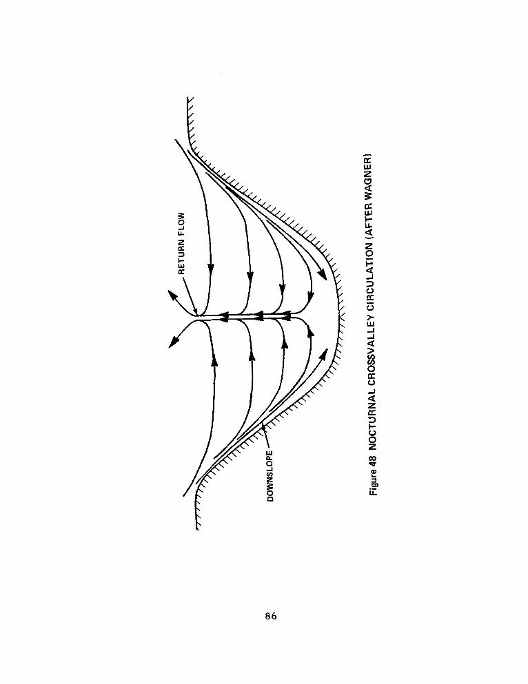
(c 1 m set’*) horizontal winds. A similar’, though.less pronounced, period i of persistent downdraft occurred at 0240 EDT..- Similar events had been
noted on previous nights before the recorder hali installed.
The bursts of vertical wind fluctuations and the persistent up- and
downdrafts are probably associated with a shifting pattern of the classical
nocturnal circulation in a valley, in .which the down slope wind stimulates
an upward return flow near the valley center before the mountain winds are / well-established (see Defant, 1951).
Between 0200 and 0400 EDT, the fluctuation rate of vertical winds
increased, but no significant changes in peak velocity occurred. Shortly
after 0400, during the period of pre-fog surface temperature rise, peak
vertical velocities decreased (with occasional exceptions) to less than -1 10 cm set . After reaching a minimum at 0430, no significant changes
occurred until fog formed at the surface.
A sharp increase in vertical gustiness occurred at 0500 EDT when
the inversion broke and fog formed. Maximum pre-sunrise gustiness was
noted at about 0600, when peak up and down motions exceeding 0.5 m set -1
occurred at intervals of less than a minute. This condition persisted until
shortly after sunrise when the frequency of the fluctuations began decreasing
and occasional peak velocities exceeding 1 m set -1 in either direction began
to occur. By the time of fog dissipation at 1000 EDT, typical maxima
exceeded 1 m set -1 and occasional peaks of 2 m set -1 occurred.
l Radiation
Radiative flux measurements were obtained at half -hourly intervals
on eleven fog days and seven no-fog days using a Suomi and Kuhn (1958) net
radiometer at the i7 m level. In addition, radiative flux measurements as
a function of altitude were &,cquired using a similar radiometer secured to a
tethered balloon (kytoon). 1 .i .:
.. ., . . .
I .
59
These radiation data were generally contaminated by the formation of
dew on the polyethylene windows of the raiaometer. Fur this reason, much
of the data cannot be interpreted quantitatively,? and are not presented here.
However, clear evening tower measurements before dew formation and kytoon
measurements before fog formation both show net upward fluxes of infrared
radiation on the order of 0.1 cal cm -2 min-i . tn. good agreement with values
in the literature.
The radiation data contaminated by dew formation show a strong
reversal in the direction of the net radiative flux about one hour after sun-
rise, even in dense fogs, supporting the sunrise effects noted in the
tempe’rature data, the dew point data, and the dew deposition data.
While the radiation data acquired from kytoon flights were generally
too noisy to analyze for radiative flux divergence, measurements obtained
in the 12 September 1970 fog at 0630 show a large radiative flux divergence
near the measured fog top at 120 m. This flux divergence corresponds to a
radiative cooling rate of approximately 4OC hr -1 in good agreement with
values computed from the recently developed dynamic fog model.
FOG MICROPHYSICS DATA
l Drop-size Distributions
Measurements of fog drop-size distribution were obtained using a
modified Bausch and Lomb slide projector to expose gelatin-coated slides
to a stream of foggy air. In operation, droplets in the air stream were
impacted on the treated slides to leave permanent, well-defined “r,eplicas”
that could be accurately measured under a microscope. Previous work
had established that true droplet diameter is very nearly equal to one-
half the diameter of the crater-like impressions left in the gelatin.
The apparatus used at the tower site was constructed to permit
control of exposure time from less than 0.1 set to periods of several
minutes and selection of air stream velocity (by a speed control on the blower
motor) between 10 and 70 m set -1
. To provide for greater accuracy in
applying collection efficiency corrections, air velocity was measured for
60
each exposure of the four millimeter wide slides. A similar drop sampler
was installed in the nose of the Aztec to permit collection of drop samples
aloft.
Data reduction was performed manually from photomicrographs obtained
with a phase contrast microscope. Where possible, a minimum of 20.0 drop-
lets was measured for each distribution. In some cases with very low drop-
let concentration, all replicas on the slide were measured directly through
the microscope. A total of approximately 200 surface (3 ft level) drop-
size distributions from eight fogs was analyzed. A similar number of
samples obtained aloft was analyzed.
Inspection of the drop-size distribution data obtained at Elmira
suggests that droplets smaller than 1 urn radius could not be detected in
the field even though smaller droplets can be detected in the laboratory.
The principal known sources of error in these measurements are statistical
in nature and imposed by the time required to measure larger numbers of
replicas for each distribution. These errors are particularly important for
small droplet sizes (< 3 urn radius) where the number of replicated droplets
is limited by small collection efficiencies and consequently collection
efficiency corrections are large (Langmuir and Blodgett, 1946). Similar
problems occur for large drop sizes where natural concentrations are
small. A second type of statistical error is due to the lack of “represen-
tativene s s ” of the sample. A fog that occupies several tens of cubic
kilometers is often characterized by a few tens of samples, each containing
the droplets from five to ten cubic centimeters.
While exposure time for a given sample is controllable, short
exposure times (CO. 5 set) are not reproducible to within a factor of about
three from slide to slide. Therefore, normalized drop-size distribution
data can be obtained directly but it is not feasible to obtain direct measure-
ments of drop concentration from the droplet samples. Drop concentrations
were obtained by combining the normalized distributions obtained at the
surface (3 ft) with simultaneous measurements of extinction coefficient
obtained from the tower transmissometer (at the 4 ft level N 100 ft away)
according to the following expression.
61
B transmissometer = 25rn g ~ i = o N(ri) ri2
where N(r) is the normalized distribution and n is the concentration. *
._ S..~ . In all cases in which drop samples were obtained from shallow ground
fog, the transmissometer was above the fog top. The visibility within the
ground fog was therefore always much less than the transmissometer
indicated. The size distributions are therefore presented only in normalized
form. Data for later periods in the fog life cycle are presented as absolute
size distributions.
If measured values for N(r) are used to compute n with typical
visibilities measured when GF exceeds the transmissometer height (4 ft),
values of n ranging from 100 to 200 cm -3 are obtained. These values are
in good agreement with the model for radiation fog developed on this pro-
gram (Jius to, 1964) which was based solely on published data. Measured
N(r) is also in agreement with model size distributions.
The surface drop-size distribution data obtained on fog nights between
the time of formation of shallow ground fog (GF) and the time of the first
visibility minimum after the formation of deep valley fog reveal a strikingly
consistent behavior. Normally, two or three GF samples were taken randomly
when GF was first observed. When deep fog began to form, samples were
usually acquired at 5- to 15-minute intervals. On 2 September 1970, however,
Attempts were made to obtain drop concentration data directly using a photographic technique similar to that used with the thermal diffusion cloud chamber. In this apparatus, a 70 u set long, 200 watt second pulse of light from a xenon flash tube was focused into a 2 mm wide ribbon in the camera field of view. The flash tube was triggered synchronously with the camera so that oint images were obtained’from light scattered by droplets in the 0.2 cm P sampling volume. Difficulty in maintaining operation of the instru- ment in the saturated atmosphere prevented acquisition of extensive data. Furthermore, with the small sampling volume, the number of images obtained per sample was so small (1 to 5) that the data were statistically poor. The data available were in general agreement with concentration data obtained in the above-described manner.
62
it was recognized from the real time display of temperature variations with
height and time that formation of deep fog was imminent and therefore a
sequence of closely-spaced drop sample collections were initiated before
substantial visibility changes were observable. As a res’ult, the most
complete data onthe evolution of the drop-size distribution in valley fog
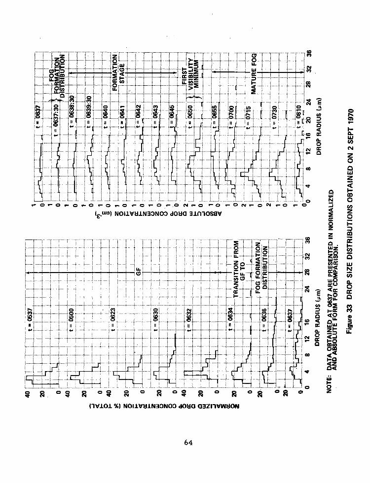
were obtained on that date. The results are presented in Figure 33. I
The drop-size distr,ibutions obtained prior to 0632 are characteristic
of all distributions obtained in shallow ground fog (i. e., a fairly large number
of very small droplets). At 0630, we observed the initial formation of fog
aloft and began sampling at 2-minute intervals. Seven minutes later, the
first decrease in surface visibility was noted and the sample interval was
decreased to one minute or 30 seconds when possible.
The distribution obtained at 0637:30 is characteristic of the distri-
butions obtained at the time of the initial surface visibility decrease on all
fog days. Data obtained between 0634 and 0637 show the transition from
characteristic GF distributions to what we have named the “fog formation
distribution”. On this date, the fog formation distribution persisted for
only a few minutes. On one occasion, 26 August 1970, however, that
distribution persisted for 45 minutes before dense fog formed.
Data obtained between 0638:30 and 0650 illustrate the changes in
drop-size distribution that occur between the initial visibility decrease and
the first visibility minimum. These changes include (1) the disappearance of
droplets smaller. than 3 or 4 pm radius, (2) the gradual increase in drop
concentration to maximum, and (3) an increase in the maximum drop size
to the largest values observed throughout the fog life cycle.
The very small droplets reappear shortly after the first visibility
minimum. From that time on, however, the behavior of the drop-size
distribution with time is not always complet.ely consistent. In three of the
eight fogs sampled, all distributions obtained at the surface after the first
minimum were similar to those shown for 2 September 1970 between 0700
and 0810. On three other occasions, surface drop-size distributions
obtained after the first minimum were predominantly bimodal, with a maxi-
mum near 2 to 3 urn radius and a second maximum in the 6 to 12 urn region.
63
. . .._
......
.... i .._
..
0 4
8 12
16
24
36
DR
OP
RAD
IUS
(pm
)
1 j__
f
. i . . . . .
. . I . . j ._
____
i . ..
__
j ____
__
j. .._.
__
i ..__.
. L _
.___
_:
____
__.
i ._._
._
j ____
._.
i . ..__
_ i..
. ..i . .._
__.
_....
. i
0:
e :_
p.. ..
__
~ i ..
_.
;... i
i t=
(-J&j
g..o
i !
;I; I
.; &i
- - :
-i yx
xy.y
. . .
. . . . .
i _
._._
i .___
__
i __.
__.. i .
. . . . i.
. :
: :
: :
: i
,..j.
. . . . .
j . . .
. . . f
= g = 4 _
_._.
4 ._
____
i _
____
_ 4 _
_....
i
j j
j : j
:-.
j i,
:. . . . .
.~
..~‘.&
.i.‘.
. . t
+ . . . .
I... ..
j ..__
__
I __.
....
( 2
” :
-:“--.
..!...
w
a
.I . . . . .
. . ‘.
F?+q
+..,i
. :
. .._.
I ___.
_,
i __.
.._
i ___
___j
__
____
I..
. . ..I .._
___
I___
_..
j !
j j
: :
7+-+
~ /
i :
/ :
DR
OP
RAD
IUS
(pm
)
NO
TE:
DAT
A O
BTAI
NED
AT
063
7 AR
E PR
ESEN
TED
IN
NO
RM
ALIZ
ED
AND
ABS
OLU
TE
FOR
M F
OR
CO
MPA
RIS
ON
.
Figu
re 3
3 D
RO
P SI
ZE D
ISTR
IBU
TIO
NS
OBT
AIN
ED
ON
2 S
EPT
1970
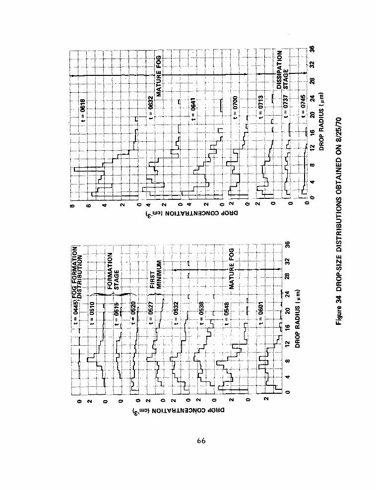
Typical distributions ofthis kind.are illustrated in Figure 34 (for times
after 0538). ‘On two*occasions, .distributions of both kinds seemed to occur
randomly through-the fog life .cycle.
The.re appear,ed to:be no consistent change in the shape of the surface
drop-size distribution as-sociated with fog dissipation. As indicated in
Figure 34, the concentration of droplets in each interval simply decre.ased
as visibility improved.. These characteristics are further illustrated in
Figures 35.and.36 which present data acquired on 22 August 1970 and
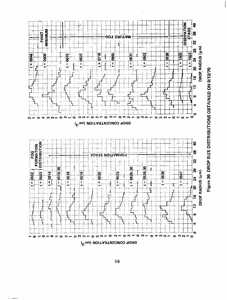
12 September 19.70,
0 Liqucd Water’ Content
-Liquid water content data were acquired by integrating the absolute
drop-s?-ze distribution (w = 4/3rrn FE i= 0
N(ri)ri3) for each drop sample and
* occasionally (5 to 10 times/fog) by direct measurement using a Gelman
high volume sampler for mechanical collection of the water from 8 m3
of fog. Cellulose filters were used in the Gelman so that liquid water was
absorbed into the fibers. To minimize the error due to absorption of water
vapor from the humid atmosphere by the cellulose, the filters were
moistened by collection of water and vapor from 2 m 3 of fog prior to the
first weight measurement. The increase in weight after exposure to an
additional 8 m3 of fog was used to determine LWC. Simultaneous measure -
ments of LWC by the two methods are compared in Figure 37. In general,
the two procedures agree to within f40 mg m -3 , which is quite good for
measurement of LWC. Variability appears to be random and is undoubtedly
associated in part with the fact that Gelman data were obtained from an
average of 8 m3 of fog acquired over a ‘I-minute interval while the drop-
.size distributions were acquired from a few cubic centimeters of fog
collected essentially instantaneously.
Complete summaries of the surface microphysics data, including drop
concentration, liquid water content and mean, mean squared, and mean volume
a( Gelman Model No. 16003
65
.... ..i
..
tS
._* ...
... j.. ...
.. . ....
.. . .....
.
n ...
......
......
... /
: ;
~:I~
:....:
~..~
::..::
::.:::
~::::
::~:::
::~:::
::~:::
::~
i .....
......
...
i .
/.~ __
_. i .._
___i
____
__
i.....
. i.
___.
._
i ___
... i ._
__.:
.i i
i j
i i
i ._...
. I . . .
. ..j
i j
0 4
8 12
16
20
24
28
32
36
DR
OP
RAD
IUS
(pm
)
0
0 4
8 D
RO
P R
ADIU
S (jd
Figu
re 3
4 D
RO
P-SI
ZE
DIS
TRIB
UTI
ON
S O
BTAI
NED
O
N 8
/25/
70
. ..~.
t’ f . .
. . . . .
: t
: i.
.I... ..
i r+
j
4 j
: :
-1
: :
: :
: :
: ..j
: ,. i
..i
? .;.
. .t
: i
i .
m
:
.’
: /
.i.
i t
._...
it &
m2&
. . .
. ~.
;.
FOG
_.
... T
. . . . .
:...
:. : +
i _ F
OR
MAT
ION
:
; DIS
TRIB
UTI
ON
-i
~~~~
~~
: :
: :
: :
. . _
. . . . .
: . . . . .
. . .
: ~
I..
/. i ..
___.
: .._._
.. ,..._
. ~ . . . .
. . . ..
_, h.
:
12
16
20
?4
28
32
DR
OP
RAD
IUS
(pri)
; /.
i . .
.+
+ :
: . .
. . .
.“‘t..
.” i
* j.,
.,...
i i
+.
~ . .
.“‘.
+A..+
:.
:
’
0.
4 8
12
16
20
24
28
32
._...
._
i ..__
__
I .._
kL!..
.?l k
iA:.L
.-Y-i-
i 1
12
16
20
24
28
32
DR
OP
RAD
IUS
l&m
) ‘D
RO
P R
ADIU
S (I.
tmk
Figu
re 3
5 D
RO
P SI
ZE D
ISTR
IBU
TIO
NS’
OBT
AIN
ED
C)N
8/2
2/70
1 0 1 0 1 0 1 0 2 1 0 3 +-
5 2 1
Go
0 3
t 2
K 1
s 0
E 8
2 E
’ *
0 8
2 E
’ 0 ;
i..
: :
: i
; i..
j
/ F
,. :
: :
j..
j /
y..+
f
i..
: :
: /
i----
--r-
i--
1--
i __.
...
4..
Ii 0 4
8 12
16
20
24
28
32
D
RO
P R
ADIU
S (IL
m)l
+.
i ;..
.t i
i :
: /
.( . . . .
. . . I
: :
..: .
.1...
...
j t
i i
: :
: ;
j /
/ .r.
. ..v.
..+ . . ..
-.....
( :
j j
i /
in
i j
i i
.+.. i
..j ._
i . .
. . ..t
( :
j .$
.. ; .
_....
; . . . . . .
. . . . .
._.
j !
..:..
_.f..
...i_
__..;
.
i j
; j
i j
/ j
: :
i i
i ,,,
I (q
----Y
- (
3P
46
DR
OFf
RAD
IUS
(pm
) ,
. .
Figu
re 3
6 D
RO
P SI
ZE D
ISTR
IBU
TIQ
NS
OBT
AIN
ED
QN
g/1
2/70
240 .-------,-------.-------~------.-------~-----~------:------,-------.------ c----T--- 1 I : I , I I I I : : 1 i 1 2 I I I I t I : I I I : ) : : 8 I i I : :
/q i. I ,------:------.-------:-------~------:--------I-------~-----. I Y-7 m’------- a I I : I I
i I i I I
: I I I : I 8 , /+( i/i i I I I I
200: I I
,-------:------~-------:------:-------i------’ I 1
; ; , ; , j-------i-------;------j ---. Y: I
I I I I I I I 8 I I I I , / I I I , I I *---,---L------:-------I id -__- I _-___- k..i _--_-. L----,-------:------~-------I I
16(y i --_^___; i ; ; ------,------:------.--------~------
I t I
; p----i ---- # ^--- j-;
LWC (mg mm31 GELMAN FILTER TECHNIQUE
Figure 37 COMPARISON OF LIQUID WATER CONTENT MEASUREMENTS MADE WITH A GELMAN HIGH VOLUME SAMPLER AND SIMULTANEOUS VALUES OBTAINED.BY INTEGRATING THE ABSOLUTE DROP-SIZE DISTRIBUTBOl-t!
69
._ - _-._ ~-- __-.---~ ---- I_~_
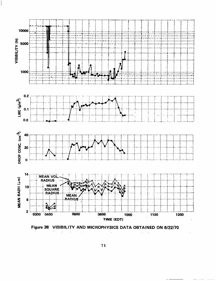
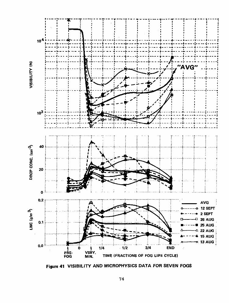
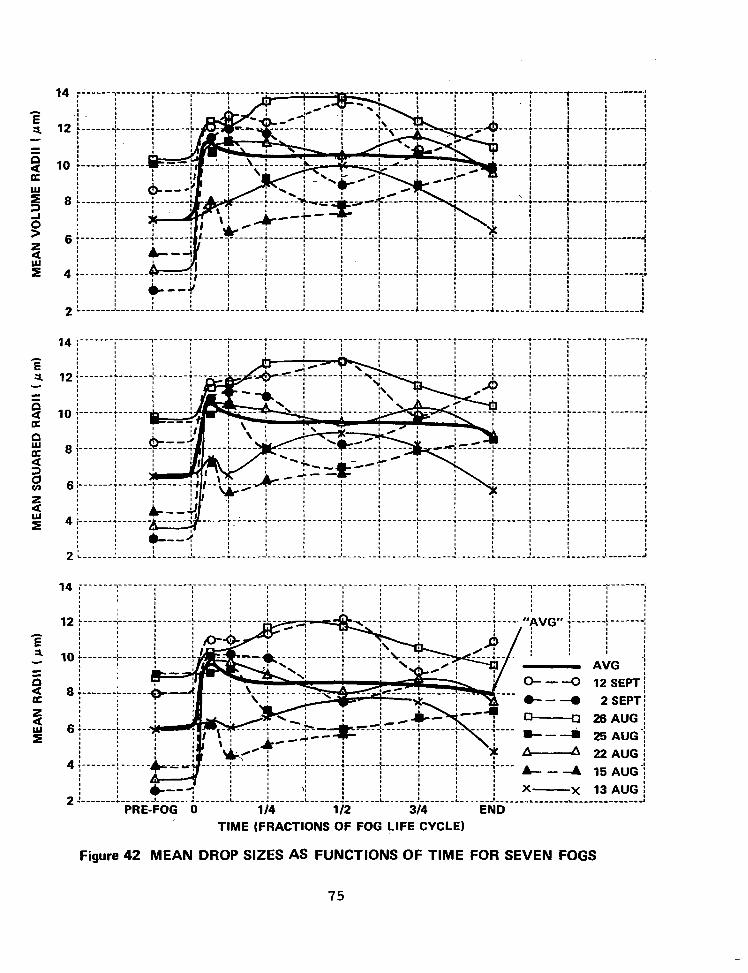
droplet radii with time are presented for the’three sample fogs in Figures 38,
39, and 40.,. The tower site visibility trace is reprinted on each figure. Note
that in Figure 40 (2 September 1970) the time scale has been expanded.
These three figures taken together illustrate the pertinent features that
are characteristic of the microphysical data throughout the life cyde of most
Elmira valley fogs. These may be summarized as follows:
i. Visibility decreases to a minimum during the first quarter of
the life cycle and then increases somewhat. Through the middle half of the
life cycle (the mature fog), visibility may remain nearly constant or undergo
large fluctuations. The dissipation stage accounts for the last quarter of
the life cycle.
2. Droplet concentration and liquid water content increase to a
maximum at the time of the first visibility minimum, fluctuate synchronously
with visibility during the mature stage and decrease drastically during the
dissipation stage.
3. The mean, mean square, and mean volume radii of the drop-size
distributions increase to a maximum approximately midway between the first
observable visibility decrease and the first visibility minimum. The mean
sizes then decrease slightly at the time of the first visibility minimum and
retain near constant values through the mature stage 0 There appear to be no
consistent changes associated with the dissipation stages.
l Summary of Surface Microphysical Properties of the Fog
Since the principal variations in fog microphysical characteristics
at the surface occur during the first and last quarters of the life cycle regard-
less of total fog duration, we attempted to model all microphysical data on a
time scale defined by fractions of total fog duration. Averages of all available
data from each fog were computed for each phase of the life cycle, with the
first visibility minimum placed at t = 1/8 total life, a reasonably representative
time. These data, together with the overall averages for all fogs are presented
in Figures 41 and 42. The figures therefore summarize all surface micro-
physical data obtained during the program with the exception of that for the
0 0 2 4 6 8 10 12 0 2 4 6 8 10 12 6 8 MEAN DROP RADIUS (ccm) MEAN DROP RADIUS (pm)
Figure 45 VARIATIONS OF MEAN DROP RADIUS WITH TIME AND HEIGHT
79
l Cloud Nucleus Observations
The CAL aircraft was used to obtain measurements of cloud conden-
sation nuclei (CCN) at several selected altitudes prior to fog formation.
Observations ‘of CCN at 0.3%S* were made at the surface and at altitudes of
30, 90, 150, and 300 m. Flights normally were scheduled at midnight,
0300 and also 0600 if fog had not already formed.
In Figure 46, average cloud nucleus data are shown for the three
flight times . Data obtained on 12 flights were used in tabulating the averages although fewer flights were possible at 0600 due to some early
occurrences of fog. The data show that cloud nucleus concentration is
highest near the ground and systematically decreases at higher altitudes in
the valley. It is of some interest to note the abundance of cloud nuclei that
are present even in the relatively clean rural environment near Elmira,
New York. By comparison, measurements of average CCN in the vicinity
of the industrial area of Buffalo, New York over a three-year period were
nearly the same or about 1000 cm -3 at 0.37~s (Kocmond and Jiusto, 1968).
No large differences in the CCN concentrations were found between the fog
and no fog flights. Since the population of fog drops ,is always much smaller
than the population of nuclei activated at 0. 37&S, this result is not surprising.
We did not attempt to measure CCN in fog since there is reason to doubt the
accuracy of such observations at high relative humidities (Saxena et al.,
1969; Fitzgerald, 1970).
Possibly a more sensitive indicator of variations in the spectrum of
“large” and “giant” nuclei that participate in fog formation can be found from
the use of the haze chamber. This device, which received only limited use
in the field this summer, is similar in most respects to the thermal diffusion
cloud chamber, the only difference being that saturated solutions of KNO3
are used in place of the upper and lower water reservoirs. It is possible,
therefore, to produce controlled relative humidities in the range of 95%-
loo%, thereby “activating” only the largest and most favorable cloud nuclei.
The data in Figure 47 show results of observations of haze and cloud
nuclei on 10 and 12 September 1970. The wide differences in haze nucleus
concentration on these two dates is particularly noteworthy, especially since *
S = supersaturation 80
$JofJ _______; ------ ~‘ !T - -- 7 ---- >;‘--:
: ---_; I I
___---
f I I
------ -----
1 I . ; : ------: :. I T : :- ,
CLOUD NUCLEI bn”)
Figure 46 VERTICAL PROFILES OF CLOUD NUCLEUS CONCENTRATION AT THREE TIMES - AVERAGE DATA FROM. 12 FLIGHTS AT S = 0.3%
a.1
0 -96 98 loo
SlS70 0260 EDT 412-70 0000 EDT
t 912-70 O!iOO EDT i
9-12-70 0700 EDT : :
102 104
RELATIVE HUMIDITY (%I
Figure 47 HAZE NUCLEI DATA
82
the CCN count at 0.370,s was nearly the same on both days. On one of the days,
12 September, .ground fog formed at about 0350 EDT and widespread dense
fog developed by 0500 EDT. Prior to fog formation, the haze. concentration
at 997’0 RH was about 40 cm -3 ; later, after fog had developed, the count fell -3 to<iCjcm . Still later in the period, after fog had persisted for several
hours, no haze nuclei at all were observed in the chamber. These data sug-
gest to us that many of the haze nuclei observed earlier in the day contri-
buted to the formation and persistence of droplets in the dense fog that later
developed at the airport. Unfortunately, no additional observations were
made after fog dissipation. In future field programs, we intend to examine
the haze nucleus concentration more carefully prior to, during, and after
fog formation. The hope is that, for the first time, measurements can be
made of the concentration of those nuclei that actually produce fog droplets.
83
CHAPTER III
DISCUSSION .OF EX-PERIMENTAL RESULTS
0 Fog Fo.rmaAion Processes at Elmira
Numerous authors have concluded that .deep fog cannot be produced
by cooling from below. Taylor (1917) concluded that turbulent transfe‘r ,df
he,at to a cold surfa.ce could not form fog and explained some advection’fogs . on the basis of. mixing of warm and cold air masses. Several authons, for
example Emmons and Montgomery (1947), Lyons et al (1962), concluded
that fog was formed as a result of radiational cooling of the moist air.
Rodhe (1962) emphasized the importance of turbulence in fog formation but
showed how radiation also contributes. He suggested that two or more pro-
cesses are usually involved in the formation of deep fog.
The observations made in Elmira and the -computer. model experiments
discussed in Chapter IV suggest that two or more processes are indeed in-
volved with the formation of deep fog in the Chemung River Valley. The
model and the data both s.uggest that the ground fog, ranging in depth from
a few centimeters to a few meters, results from caoling of the air by
diffusion of heat to the. cold -ground. The fact that the deep fog forms first
aloft, with its .base at-least..30 ,to 60m above th-e surface, indicates that
some process other than the-turbulent transport of heat to the surface is
involved.
Examination of the Elmira data, together with the model calculations
and previously-published information, provides some insight into what these
mechanisms may be. We can not describe these mechanisms in a pre-
cise manner, however.
Several authors who concluded that eddy diffusion could not produce
sufficient cooling to cause-deep fog have already been referenced. In Our
modeling experiments, we were unable to produce significant cooling. above
a few tens of meters without assuming unreasonably high transfer co-
efficients. In fact, those conditions which produced even slight cooling
at the 1OOm level produced unrealistic low-level temperature profiles
and never produced even a thin ground fog. The empirical data show,
however, that the maximum cooling rates during the last six hours before
fog formation occur in the vicinity of 100m. -Obviously, some other cooling
mechanism must be responsible.
84
:It seems most reasonable that the temperature distribution leading
to the”,formation of a valley fog is a result of the nocturnal valley circul-
ations described by Defant (1951) on the‘.basis of the work of Wagner (1931,
1932, .1938). Radiative coc,ling of the slopes stimulates. the downslope
wind and its upward return flow in the center valley region as illustrated
-*‘Figure ~48 . This proces.s, which begins within an hour after sunset
(Geiger., 1965, Chapter VII) certainly contributes to the formation of the
-deep nocturnal inversion. Several hours after sunset, the so-called
mountain wind is established by-drainage of the cool air in the direction
of the axis of,the valley. The- speed of the mountain wind is usually maxi-
mum (2 to .4 m set-‘) at 1 evels ranging from 40 to 200 m. As the mountain
wind is generated, the upward motion in the center of tl-e valley dies, but
the downslope .wind persists as shown in Figure 49. During the late night
hours , the downslope winds cease so that the mountain wind occupies thi
entire valley and persists until after sunrise.
It is attractive to speculate that the cooling at all levels within the
valley until approximately three hours before fog formation results from
the upward flow of cool surface air in the center valley region. At
ab.out that time, .the mountain wind is initiated (see Geiger, 1965, Chapter
VII) and retards the up.ward motion in the center valley region so that the
cooling rate. at higher levels is decreased without significantly affecting
-cooling at lower and mid levels. This is reasonable, since the downslope
wind must provide the most cold air at the altitude of maximum mountain
wind speeds. Qualitatively, therefore, the temperature-time relationships
depicted in Figures 17 and 18 should result.
If we postulate further that the dew point inversion extends to
,significantly higher altitudes than the highest measurements made in Elmira
(i. e., 17m), fog would form first aloft. Justification for this assumption
.is presented in the next subsection. Further justification was found by
Schuepp (1-945) in the only known simultaneous investigation of temperature
.and moisture distributions and valley circulations. He reported that on the
average, a tongue of moist air extended from the slopes to the center of the
;Davos Valley in Switzerland at an ‘average height of 40m, the same altitude
85
RET
UR
N
FLO
W
Figu
re
48
NO
CTU
RN
AL
CR
OSS
VALL
EY
CIR
CU
LATI
ON
(A
FTER
W
AGN
ER)
a b
a. DDWNSLOPE WIND BEGINS SHORTLY AFTER SUNSET BEFORE UP-VALLEY MOUNTAIN WIND DIES:
b. IN LATE EVENING UP-VALLEY WIND DIES AND ONLY DOWNSLOPE WIND AND RETURN FLOW AT CENTER OF VALLEY EXIST.
c. RETURN FLOW AT CENTER OF VALLEY CEASES AND DOWN- VALLEY MOUNTAIN WIND BECOMES ESTABLISHED.
d. LATE AT NIGHT THE DOWNSLOPE WIND CEASES AND THE DOWN-VALLEY MOUNTAIN WIND PERSISTS.
Figure 49 THE NOCTURNAL MOUNTAIN WIND (AFTER DEFANT)
87
as the maxima of the valley wind.;for-the experimental pe.riod. Schuepp%.
data are presented.in Geig:er @965; Chapter; VII)
Once fpg has formed:aloft,, the propagation o.f>‘its bas.e downward is
readily explained-by an extension of ‘the .ideas suggested-by:Fleagle: et a?.
(1952) concerning changes in stability that occur.as a result- of ra&ative
flux divergence at the fog- top. Assuming that na.heattransfer occurs at
the fog boundary, Korb and Zdunkowski (1970) calculated the cooling due to
the flux divergence of a 1’. 6 m thick fog layer with a LWC = 0.1 g/m3 to
be approximately 9OC /hr ; Such a cooling r.ate tends to increase the stability
at and immediately above the fog top and causes an unstable lapse to exist
within the fog. In the case of fog aloft, the instability must eventually extend.
beneath the fog base,. As -a result, -the cold foggy air mixes predominantly
with the clear, almost saturated air beneath to cause saturated conditions to
propagate downward.
As mixing causes the supersaturated region to grow d0wnwar.d and
fog forms at lower levels, condensation and evaporation that -accompany up and
down motions must cause the lapse rate beneath the level of maximum radiation
divergence to approach wet adiabatic.
To summarize, therefore, we believe that the mannerin which deep
valley fog forms is as follows: (1) Nocturnal radiation from the surface
and subsequent turbulent heat transfer from air to ground which produces
an initia 1 low- level temperature inversion stimulates. the downslope
wind and the upward return flow near the valley center. During this perrod,
dew deposition at the cold s.urface,creates the low level dewpoint inversion.
The upward motion at the valley center carries the cool and some-what dry
air aloft to cause the inversion to deepen. (2) Approximately three hours.
before fog formation, the mountain wind.forms and restricts the-upward
motion of air near the valley center. Cooling is therefore restricted to
low and mid-levels of the valley; i. e., those levels in which fog will event-
ually form . The continuing downslope wind, which provides cold air for
the mountain wind, mixes with existing, warmer air at mid-levels in the
valley and causes the cooling rate to,maximize in that region. Through
this period, the dewpoint inversion persists. Temperature and dewpoint,
88
therefore, converge at mid-levels, and two to three hours’ after formation
of the mountain wind, a thin layer of fog forms aloft. (3) The divergence
of radiation in the fog simultaneously increases the stability at the fog top
and promotes unstable’,conditions at the base of the thin fog layer aloft.
Cool, foggy air therefore mixes with the clear air immediately below and
causes supersaturation to propagate downward. This process continues
until the fog base reaches the surface.
When fog forms before sunrise, the surface warming that begins
between one half and one hour before sunrise is a result of a decrease in
net radiation from the surface caused by the fog forming aloft and the con-
tinued conduction of heat from subsurface levels. The warming is repro-
duced quite well by the computer model.
When fog has not yet formed by sunrise, the surface warming and’ ,
accompanying dew evaporation is caused by the sun. The instability that
results at low levels stimulates vertical motions which apparently cause
the now moist air from low levels to mix with cooler air aloft and produce
the supersaturation that results in fog formation. Apparently this process
produces fog after sunrise only when nocturnal processes have produced a
very delicately balanced set of atmospheric conditions in the valley,
since post sunrise fog formation occurred at the airport on three occasions
and formed in other parts of the valley but not at the airport on two other
seemingly identical occasions.
In reviewing the processes of fog formation, other ‘mechanisms
were examined in attempts to explain the observed temperature changes
that occur in the valley. The mechanisms include direct long-wave radiative
flux divergence from the upper atmosphere, horizontal eddy diffusion to
the valley walls, and advection of cool air over the vsilley from the adjacent
hilltops. As indicated in the subsequent paragraphs, these mechanisms are
either inadequate to explain the observed cooling rates or produce temper-
ature distributions that are in conflict with the data.
Kondo (1971) estimated the low-level cooling due to long-wave radi-
ation under atmospheric conditions similar to those encountered in Elmira,
89 -
__- ._-.~-I-. I - - - - - . . . - . . - - . -
~-- -
1. e., low wind speeds and high humidity at slightly warmer than freezing
temperatures. His results indicate that long-wave radiation is indeed i -
important to the heat budget in the lowest 100 m. Maximum cooling rates
( 1.2,: C hr”) occur in the fowest meter of air and cooling rates at the 100 m
level between midnight and 0600 are of the order of 0.2’ C hr -1 . The
observed vertical distribution of cooling at Elmira is therefore reversed
from that predicted on the basis of long-wave radiation.
Order of magnitude calc,ulationsshow that to produce the observed
cooling rates through horizontal eddy diffusion to the valley walls with the . . maximum observed temperature difference between hillside and center
valley would require horizontal.diffusion coefficients at least two orders of
magnitude greater than expected under the stable conditions that exist before
fog formation. Hence, horizontal diffusion must be eliminated as a cooling
mechanism.
Advection of cold air from near the hilltops with the cross valley
component of the ambient wind certainly contributes to cooling aloft. During . the early evening, this process may be viewed qualitatively as an eddy dif-
fusion process in which the ambient wind is blowing across an extremely
rough surface consisting of the Chemung’County hills. Such a mechanism
could be responsible for the deep inversions (illustrated in Figures 15 and
16) which form before midnight.
The hypothesis that this cooling mechanism is responsible for fog
formation breaks down upon consideration of the observed vertical’ temper-
ature distribution after midnight and the correlation of that distribution
with eventual fog height. Advection of cold air over the valley from the
hilltops would cause maximum cooling near the hilltop levels or 200 to 300 m .
above the valley base. The data show,. however, that the rate of cooling
decreases at these levels several hours before fog formation, while the
maximum cooling persists at or below 100 m in a manner that is correlated
with eventual fog height. The data indicate, therefore, that the air in
which the fog ‘will form becomes more and more isolated from the air
advecting over the valley from-the’ hills in the hours immediately preceding
fog formation.
90
0 The Role of Dew in the Fog Life Cycle
The downward transport of moisture on clear nights and the for-
mation of the nocturnal dew point inversion are attributed by numerous
authors to the deposition of dew at the surface’.’ ’ See Wells (1838) and
Geiger (1965, Chapter II). The first question he&ining to the role of dew
in the fog life cycle is whether or not sufficient moisture is extracted by
dew to produce the deep inversion postulated in the previous subsetition.
Geiger presents empirical and theoretical data from a number of
authors indicating that the nocturnal dew point inversion frequently extends
to between 40 and 200 meters. The dew point inversions observed by
Schuepp to extend to the 40 m level in a valley were already referenced.
On the basis of past work, therefore, the assumption seems reasonable.
Our numerical model predicts dew point inversions extending to 40 m only
with exchange coefficients too large. to permit formation of fog. It must
be recalled, however, that these same large exchange coefficients were
required to produce temperature inversions extending to the same levels.
Obviously, therefore, the numerical model does not simulate the valley situation
adequately.
Some direct evidence that the prefog dewpoint inversion extends to
upper levels in Elmira may be derived by combining our low-level dew
point and dew deposition data.
If the observed dew is formed entirely as a result of extraction of
water vapor in the atmosphere at the starting time and air mass changes
do not account for observe? dew point changes, conservation of mass may
be used to provide an order of magnitude estimate of the depth of the, dew .I. . . point inversion if it is assumed that the initial and final dew point profiles I are linear. The results of such a calculation based on the average data
presented in Figures 26 and 28 and illustrated in Figure 50 indicate an
inversion depth of 200 m. Even if 50% of the observed dew was formed
from water vapor evaporated from the relatively, warm soil (beneath the
cold upper surface of grass) during the observation period (see Geiger,
1965, Chapter II) the depth of the inve,rsion is more than adequate to explain
200
180
160
140
60
I 0 -.
I -. ------~------:-------:-------i-------.------i-------*------~--
-.
O- 0 w 4 8 10 12 14 16 18
DEWPDINT (‘Cl
Figure 50 CALCULATED DEW POINT CHANhE BETWEEN t = -6 HOURS AND t = -0.5 HOUR REQUIRED TO PRODUCE MEASURED DEW DEPOSITION IN SAME TIME INTERVAL 92
inversion heights in the 30 to 60 m range. With the temperature distribu-
tion approaching isothermal beneath these levels, fog forms first aloft.
Between the time of fog formation and sunrise, it appears that dew
serves no function-other than to provide a wet lower boundary for thevalley
fog. After sunrise, the role of dew is most important.
Shortly after sunrise, the surface temperature begins to increase
and stimulate dew evaporation. During the second hour after sunrise, the
temperature of the entire fog increases at an average. rate of 0.7” C hr -*. It
is necessary, therefore, to provide water vapor to the fog at a rate of
0.4 g m -3 hr-l simply to maintain saturation. During the same period, the
average dew evaporation rate is 55 g m -2 hr-l , which is sufficient to main- tain saturation in a fog 140 m thick. The fog, therefore, persists.
During the third hour after sunrise, the average rate of heating of
the fog gradually increases to the point where dew evaporation can no
longer maintain saturation. One should, therefore, expect fog dissipation
to begin between 0830 and 0930 local time. The average observed time of
the beginning of dissipation was very near 0900.
From these simple quantitative observations, it is apparent that dew
evaporation plays a major role in the persistence of valley fog after sunrise.
As indicated above, natural fog dissipation begins when dew evap-
oration is not adequate to maintain saturation at a rate consistent with the
rate of temperature increase. It is readily apparent from even casual
observations that dissipation occurs first at the surface and gradually pro-
ceeds upward; a fact which undoubtedly has resulted in the term “fog lifting. ”
For this sequence of events to occur, it is necessary for temperature to
increase most rapidly at low levels to establish a lapse rate that is steeper
than wet adiabatic beneath the persisting part of the fog. Under these con-
ditions, the fog can be maintained aloft by cooling due to the upward air
motions that occur at the time of fog dissipation (Figure 31).
Our tower temperature data indicate a superadiabatic lapse in the
lowest 17 meters through fog dissipation. Our aircraft temperature data
are not sufficiently accurate to distinguish between a wet adiabatic and the slightly greater lapse needed to explain ‘fog lifting. ”
93
l Evolution of Drop-Size Distributions and Associated Implications .
i The experimental data presented in Figures 33 and 35 show that the
drop-size distributions that exist prior to formation of deep fog are consistently
characterized by a mode, between 2 -and 4 pm radius and a maximum of about
8 pm. Between 65 and 95% of the droplets in each distribution have radii
larger than 2 pm, suggesting that the observed droplets were not simply
enlarged nuclei; i. e., the nuclei were fully activated to droplet growth.
As indicated in the data ,pre sentation, these droplets characterize the ground
fog which is usually below the level of the transmissometer. For this
reason, absolute concentration cannot be established. Calculations based
on transmissometer data obtained when the beam passes through the ground
fog indicate typical droplets concentrations of 100 to 200 cm -3 .
Qur notes do not include comments indicating the presence of ground
fog immediately preceding the formation of deep fog. Through the early
morning hours, we often observed GF to dissipate and reform. We were
usually distracted, however, from the ground fog by the formation of deep
fog aloft and consequently do not know if the dense ground fog dissipates prior
to deep fog formation. From the data presented in Figures 33 and 40 for
the fog of 2 September, it appears that the ground fog droplets did persist
&til deep fog formation but that drop concentration decreased before deep
fog formed.
Changes in drop concentration may be due to a combination of the
low-level warming that precedes fog formation and to the vertical mixing
that increases significantly during the formation period of deep fog. In any
case, it is apparent that the supersaturation present in the ground fog is
sufficient to support the presence of 60 to 200 droplets cm -3 and therefore
to produce full activation of those concentrations of cloud nuclei. These
concentrations are greater by a factor of 2 to 10 than droplet concentrations
observed in the deep fog. If it is assumed that the activation spectrum of
the nuclei in the region in which ground fog forms is the same as at higher
altitudes in the valley, which is certainly reasonable, it follows that
supersaturation at the time. of formation of ground fog is significantly
greater than during formation of the deep fog.
94
This conclusion seems quite reasonable upon consideration of the
temperature distribution through the two fqg depths. Figure 13 shows the
mean temperature difference to be approximately 2.5OC between the 1 m and _. 0.1 m levels during the sixPours before fog. As,equal air par’cels from ‘.
each of these .levtils are mixed, the supersaturation developed (before vapor
depletion by dropJet growth) is approximately 0.3%. Without vapor depletion,
our cloud nuclei data (Figure 46) show that approximately 1000 nuclei cm -3
would be activated. With the existing vapor Lo’sses, the supkrsaturation
attained is Less.and apparently just sufficient to’produce the observed 100 -3 to 200 droplets cm .
The data presented in Figure 20, on the other hand, indicate a
maximum temperature difference of about 1OC during the interval in which
deep fog forms (At = one-half hour). Mixing of the two saturate.d air parcels
at the temperature extremes would produce a supersaturation slightly
exceeding 0.1% if such mixing could occur. Considering the extreme
separation of these air parcels, it is obviously impossible for such mixing
to occur without thorough dilution by air from other levels. .
While the supersaturation at the time of ground fog formation exceeds
that for deep fog, the drop-size distribution in groutid fog remains narrow
throughout its life cycle. This is partially due to precipitation of the largest
drops (e.g., a 5 pm radius droplet falls through the 1 m depth in approxi-
mately five minutes) and is also associated with vapor depletion by the high
concentration of existing droplets. Available water must be distributed over
a higher concentration of nuclei so that no one droplet can grow rapidly. For
obvious reasons, these mechanisms are not as effective in deep fog and the
equilibrium drop-size distribution is significantly wider.
The consistent pattern of the evolution of the drop-size distribution
between the fog formation distribution and the first visibility minimum is
intriguing. The fact that droplets small’er th?n 3 to 4 pm radius are never
detected during this period in which the total concentration of droplets is
increasing deserves ‘explanation. There appears to be an internal conflict
in the data; i. e. , large droplets seem to form without going through the
small droplet stage.
95
One hypothesis which was cdnsidered in attempting to explain these .
observations is that the time required for growth of a n&w droplet from its
critical radius (i.e., its radius at the maximum of the relevant Kohler
curve) to 3 pm radius is so short and the concentration of drops in the 1
to 3 pm size range at any time is so small that the probability of detection
of one of these droplets with our sampling procedure is essentially zero.
Excluding the fog of 15 August 1970, the average maximum rate of
increase in drop concentration was 0.6 cm -3 -1 min . On 15 August 2970,
the only case in which small drops were observed during the formation
stage of deep fog, the rate was 2.6 drops cm -3 -1 min . Since droplets
smaller than 3 pm radius are seldom observed, the hypothesis stipulates
that the average concentration of droplets in this range must be smaller -‘3 thanO.l cm , which is the minimum concentration that is consistently
detected (probably about 50% of the time) with our sampling procedures.
If we consider the average concentration to be a time average, it is neces-
sary that the fraction of any long-time interval during which a given cubic
centimeter of air is occupied by at least one droplet smaller than 3 pm
radius is substantially less than 0.1. Otherwise, droplets in this size
range would be detected. This fraction of the time is given by the product
of the production rate of droplets and the time T required for a newly
activated droplet to grow to 3 pm radius. To go undetected, therefore:
0.1 < 0.6 cm-’ minute x T minutes
T < 0.17 minutes = 10 seconds
We may now ask whether or not the supersaturation required to pro-
duce such rapid growth can exist near the surface during fog formation. As
a test case, we computed the growth at 0.3% supersaturation of drops that form
on nuclei with different activation thresholds. The results are presented in
Table III.
96
Table III
Growth of ,Droplets at 0.3%S
on:Nucl& of Different Activation Supersaturations
‘Radius .of dry NaCl Par.ticle
Activation Thre sho1.d
Droplet Size at Indicated Time
5 Seconds 10 Seconds 20 Seconds
‘0.02‘0 pm 0.45% 0.12 pm 0.13 pm 0.14 pm
0. 0’2’5 0.32 0.20 0.20 0.20
.0..03.2 0.23 1.17 1.85 2.82
0.040 0.16 1.31 1.95 2.90
It is obvious from these values that the time required for droplet
growth on nuclei with even significantly Lower activation thresholds than the
existing supersaturation substantially exceeds the ten-second limit established
above. .Even larger supersaturation would therefore be required to explain
the observations on the basis of this hypothesis. Since the data presented in
Figure 46 show that the concentration of nuclei activated at 0.3% is of the -3 order of 1000 cm , we know that such supersaturations do not exist in the
region of the measurement.
We must conclude from this analysis that the increase in concentration
of droplets near the surface during deep fog formation is not due to activation
,of new nuclei in the region where the observations are made.
It’is conceivable under some fog conditions that sporadic supersaturations
exceeding 0,30/o could be produced in small regions by mixing of the two near-
saturate’d air parcels with different initial temperatures. The required
tem,perature differences exceed those which were observed within the fog
at Elmira, h0weve.r.
A more realistic hypothesis for explaining the increase in droplet
concentration at the surface during the fog formation stage is that the drop-
lets are transported to the surface by turbulent diffusion from aloft. Under
this assumption, the initial appearance of deep fog at the surface could occur
97
during a period in which the surface atmosphere is slightly unsaturated.
With the fog existing aloft for times ranging from one-quarter to one hour
before the first decrease in visibility, it is not necessari to postulate such
rapid droplet growth and high supersaturations in order to cause most of
the droplets to grow to radii exceeding 3.0 pm. The generation of new
droplets can proceed continuously at higher altitudes. Upon being trapped
in turbulent eddies, the droplets are carried downward. The associated
warming promotes evaporation which tends to produce a wet adiabatic lapse.
With the driving function for evaporation under a wet adiabatic lapse being
a 0.02% supersaturation reduction per meter of descent, evaporation of
newly formed small droplets can begin even before the eddy reaches the
existing fog base.
If this level is 20 m, for example, evaporation may proceed for
periods exceeding 100 seconds at the typical downward velocities observed
on 12 September 1970 (Figure 31B) during the fog formation period. With
the lower atmosphere already slightly subsaturated, the extremely small
droplets can disappear.
The evaporation of droplets in the lower atmosphere plus the
evaporation of dew from the warming surface must cause an increase in
dew point at lower levels. (Such an increase is evident in the data presented
in Figure 26. ) When the lower atmosphere becomes saturated, complete
evaporation of small droplets no longer occurs and the small droplets
reappear in the data,.
From the bimodal drop-size distributions in some fogs, it appears
that in some cases, the low Levels become supersaturated so that additional
nuclei are activated, At the very low supersaturations that can exist in the
presence of the high droplet concentration, the newly formed droplets grow
very slowly so that it is not necessary to postulate continuous activation
of nuclei to maintain the bimodal distribution.
98
CHAPTER IV
NUMERICAL MODELING OF RADLA‘TION FOG
INTRODUCTION
l Brief Description of Model
A numerical model has been developed to investigate the influences of
various vertical transfer processes in shaping ‘the life cycle of radiation fogs,
i.le. , fogs which result from the nocturnal cooling of the earth’s surface
by infrared radiation. The model has a one-dimensional vertical grid
system which extend,s from one meter below the earth’s surface to several
hundred meters above the surface. In the atmosphere, starting from various
initial conditions, the model predicts the temporal evolution of the vertical
distributions of potential temperature, water vapor, and liquid water as
determined by turbulent diffusiori. Prior to fog formation, radiative flux
divergence in the atmosphere is neglected. In the soil, the model predicts
the evolution of the vertical temperature distribution under the influence
of heat conduction.
The atmosphere and soil are coupled at the surface by maintaining
continuity of the temperature and heat flux. During nocturnal cooling, the
net upward flux of infrared radiation at the surface is balanced by an upward
heat flux from the soil and a downward eddy flux of heat from the atmosphere.
A no-flux boundary condition on water vapor content is maintained at the
surface until the dew point is reached. Aft&r the surface is cooled to the
dew point, the water vapor content at the surface is assumed to be saturated
at the surface temperature, and dew is allowed to form.
Fog is formed in the model by converting any water vapor content in
excess of saturation into liquid water, after accounting for the latent heat
of condensation released in the process. The model includes the influences
of infrared absorption and radiation by fogj and fog drop sedimentation upon
the development and maintenance of fog.
The most difficult area in the model development has proven to be the
necessity of providing atmosphere exchange coefficients for turbulent
transfer of he&t and moisture over wide variations of height and stability.
99
Some success has been achieved in using exchange coefficients tihich are
functions of friction-velocity, height, and the predicted local thermal
stability .
Numerical experi.ments with the fog model have been devoted-to
delipeating the roles of the turbulent transfer of heat -and moisture and the.
radiative transfer of heat in the formation and maintenance of fog. The
model has been fairly successful in simulating the formation of radiation
fogs (IO-40 meters in height) starting from conditions near sundown. It
appears, however, that a considerable improvement on the realism of the
modeling results might be effected by making the horizontal wind a prognostic
variable of the model, and including a dependence of the exchange coefficients
on the vertical wind shear.
The model has not been successful in producing the deep fogs
(100-150 meters in height) observed near Elmira, New York. It is believed
that a two- or three-dimensional model will be required to provide .a
satisfactory simulation of fog formation aloft and some other characteristic.
features of the deep valley fogs. The present model, however, constitutes.
a significant advance in the modeling of the processes which shape the Life
cycle of fog and provides a sound basis for the development of-multi-
dimensional models in the future.
l Previous Work
Although the development of the present model was based upon studies
of fog, nocturnal cooling, turbulence, and radiative transfer too numerous
to cite here, it is appropriate to mention certain studies which had a’
particularly important influence on the direction of the present modeling
investigation.
An investigation of the factors which contribute to the formation of
fog is not complete without a careful study of the classical paper by
Rodhe (1962) on “The effect of turbulence on fog formation. I’ Rodhe puts
the thermodynamics of unsaturated and saturated processes on a common
basis and delineates the key role in fog formation of the simultaneous turbulent
transfer of heat and moisture. His analytical treatment of the formation of
radiation fog, although based on a constant, height independent turbulent
exchange coefficient, offers important insights in the physical processes involved.
100
Fisher and Caplan (1.963) demonstrated the feasibiIity, of simulating ,the
formation.and dissipation- of radiation and advection fogs bymeans of a
numerical’ model.. The.pres-ent model employs to a large extent the computational
procedure .used by Fisher and Caplan to solve.their differential equations for
the changes in potential temperature, water vapor content, and liquid water
co$ent produced Ey,vertical turbulknt diffusion. Fisher and CapFan use
var.&Le turbulent exchange coefficients which depend upon height and local
stability, although in a somewhat crude manner. No radiation effects are
included in the model.
A study of the Fisher and Caplan results for radiation fogs shows
that the principal shortcoming of their model Ts a predetermined temperature
variation at the surface, which does not depend upon the computed variables.
Also, their no-flux condition on moisture at the surface precludes the
development of a dew point inversion as a result of dew deposition at the surface.
McDonald (1963) proposed a “saturation adjustment” procedure in the
numerical modeling of fog to treat condensation and evaporation in a thermo-
dynamically sound manner. This procedure is used in the present model.
Zdunkowski and Nielsen (1969) discuss a fairly sophisticated numerical
model of radiation fog. Their model provides a careful, unified treatment of
the atmosphere and the soil so that the surface temperature is a prognostic
variable of the model. In the Zdunkowski and Nielsen model, the radiative
flux divergences produced by water vapor and fog droplets are predicted
through. unified radiative transfer .caLculations at every time step. Their
turbulent exchange coefficients, on the other hand, are height dependent,
but do not vary with time as a function of prognostic variables of the model.
The surface boundary conditions on moisture employed by Zdunkowski
and Nielsen conserve the total moisture content of the atmosphere. This
again precludes the formation of a dew point inversion as a result of dew
deposition of the. surface, a phenomena which can significantly delay the
formation of fog (see Rodhe (1962) ). Nevertheless, the numerical results
obtained’by Zdtinkowski and Nielsen appear sufficiently realistic to indicate
the fundamental soundness of much of the model. As noted by the authors,
the principal improvement necessary in-the development of a satisfactory
radiation f’$ model is the internal generation of realistic exchange
coefficients as a function of the prognostic variables of the model.
The primary improvements attempted in the present numerical . fog model are internally generated exchange coefficients, dew formation
at the surface, and inclusion of the effects of fog drop sedimentation.
Only a crude treatment of radiative transfer is included. The numerical
model is described in some detail in the next section entitled Numerical
Model, and the results of numerical experiments with the model are
discussed in the section entitled Results.
NUMERICAL MODEL
l Major Asstimptions
The following assumptions are adopted in the numerical modeling
study of radiation fog:
a) The model is one-dimensional in the Z direction. All of the
quantities are uniform in an X, Y plane.
b) The turbulent exchange coefficients for heat, water vapor, and
liquid water are equal.
c) Prior to fog formation, radiative flux divergence in the atmos-
phere is neglected.
d) Supersaturated water vapor condenses instantaneously until
saturation is achieved. Liquid water in an unsaturated region evaporates
instantaneously until saturation is achieved or the liquid water is exhausted.
l Equations
List of Symbols
In order to avoid lengthy explanations in the text, a list of the most
important symbols employed will be given first:
102
temperature and potential temperature of air
soil temperature
water vapor mixing ratio
saturation mixing ratio
liquid water mixing ratio
height coordinate
kth vertical grid level
time
turbulent exchange coefficient for vertical transfer
thermal diffusivity of soil
density of air and soil
specific heat of air at constant pressure and of soil
net upward flux of infrared radiation
Stefan- Boltzmann constant
air pressure
latent heat of condensation
mean terminal velocity of fog drops
ass absorption coefficient of fog for infrared radiation ;zFg3)
gravitational constant
friction velocity
Von Karman constant = 0.4
denotes nth time step
Major Equations
The equations employed in the model for the time rate change of
potential temperature B , water vapor mixing ratio r , liquid water
mixing ratio U , and soil temperature G are:
(4)
(5)
103
(6)
Saturation Adjustment
The symbol C ,denotes a source function for condensation or
evaporation. In the actual model, the finite difference-.approximations to
Eqs. (4) through (7) are integrated for a time step, neglecting condensa.tion
or evaporation. ’ Then, the saturation .adjustment procedure develo,ped by
McDonald (1963) is applied to the new valueg of B , P , and .w .
Taking into account the heating of the air by the release of latent heat of
condensation, supersaturated water vapor at a grid Level is converted into
liquid water until saturation is achieved. Similarly, taking into account the
cooling of the .air, liquid wate.r at a grid level is evaporated into an unsaturated
vapor until saturation is achieved or the liquid water is exhausted.
Radiation
The treatment of radiation in the present model is designed to cap-.
ture the essence of physical processes while avoiding detailed radiative
transfer calculations. Prior to fog. formation, the radiative fll-x divergence
2Q3z in Eq. (4) is assumed to be everywhere zero. The net upward
flux of infrared radiation at the surface R(O) is assumed to be a constant
fraction p of the blackbody radiation at the surface temperature 7(O) i.e.,
R(0) = p o- T+m (8)
The constant ,5 is typically taken to be . 25 (Sutton, 1953), signifying that
the back radiation from atmosphere is assumed to be .75 of the full blackbody
radiation from the surface.
104
After fog formation, a radiative flux divergence JR/Jz resulting
from absorption and reradiation by the fog drops is introduced in Eq. (4).
Representing the ,influence of fog drops by a single spectrally-ave.raged
mass absorption coefficient k, and neglecting temperature gradients
in the fog, the radiative flux at a height t in the ,fog is given by
(9)
where zt is the top of the fog and the effect of the angular dependence
of the radiation field has been approximated by. using the diffusivity factor
1.6 (Goody, 1964). Differentiating with respect to e , the radiative flux
divergence at height z is given by
In the model, the integrals over UY are evaluated numerically.
In the Rayleigh limit r/3( < .c 1, the absorption cross section of
water drops is proportional to f3 (Batten, 4959). The results of Stephens
(1961) show that spectrally-averaged absorption cross sections for black-
body radiation are virtually independent of temperature in the temperature
range of interest to this study, and approximately proportional to r 3 for
drop sizes up to r = 5 pm. Based upon these results of Stephens, a mean
mass absorption coefficient k ur 7.5x 1u3cm$-~ was deduced and
was applied in the model.
This treatment of radiative transfer in a fog would not be a satis-
factory approximation for a fog which has a significant number of drops
with r > 10 pm, since the spectrally-averaged absorption cross sections
for large drops are approximately proportional to r+ (Zdunkowski and
Nielsen, 1969), and scattering becomes increasingly important in the radi-
ative transfer as the drop sizes increase. It also should be noted that use
of a spectrally-averaged absorption coefficient for blackbody radiation is
less than accurate for the back radiation from the atmosphere which is
deficient in water vapor window near il = 10 pm. In spite of these
105
shortcomings, this simple treatment provides a roughly quantitative simu-
lation of the reduction of the net upward radiation at the surface by fog and
of the accompanying radiative cooling of the fog.
Exchange Coefficients
The most difficult area in the development of the model proved to be
providing realistic turbulent exchange coefficients for the vertical transfer
of heat and moisture over wide ranges of height and stability. The
preponderance of useful information in the literature on vertical turbulent
transfer is restricted to a few tens of meters above. the surface in the
“constant flux’! iayer . Furthermore, during low wind nocturnal inversion
conditions, there is a paucity of observational data on turbulence and vertical
transfer.
Observational data from Elmira in mature fogs show a transition
from unstable conditions near the surface to a capping inversion at fog top,
even at night. To treat this situation, it appeared necessary that the
turbulent exchange coefficients in the model should be a function of the
local stability, not just the surface heat flux as in a constant flux layer.
On the other hand, since the horizontal wind is not a prognostic variable
in the present model, the friction velocity LC* = $7- z p , where Z is
the shear stress, is treated as an input parameter in the model.
It is assumed in the model that the exchange coefficients for heat,
water vapor, and liquid water are equal. The functional dependence of the
exchange coefficients upon local stability and height in the model is based
upon the so-called KEYPS formula (Lumley and Panofsky, 1964)
s”- y; s3 = 1,
for the dependence of non-dimensional wind shear
kz Btv s= -- u* de
upon height z and the scaling length *3
L= -lx. pc 7- :
kYH
(12)
(13)
106
Here, j-I is the vertical heat flux and 7 is an empirical constant which
is assumed to be 14 after Lumley and Panofsky.
The KEYPS formula is an interpolation between free and forced
convection and has been shown to be in reasonable agreement with obser-
vations in the constant flux layer extending 10-100 meters above the sur- I face, where z and H are approximately constant. Assuming that the
exchange coefficients for momentum and heat are equal and that H is the
local heat flux, the KEYPS formula yields an explicit relationship for the
exchange coefficients as a function of height and stability. In the present
fog model, this relationship is applied throughout the entire depth of the
model atmosphere.
By definition, of the exchange coefficient for momentum K/77 , the
non-dimensional wind shear can be written in the form
ku’z s= -y- m
(14)
By definition of the exchange coefficient for heat Kh , the vertical heat
flux is
(15)
Substituting this expression for // into Eq. (13), the scaling length
can be written
Now substituting Eq. (14) and Eq. (16) into KEYPS formula, Eq. (II), and
asserting Kh = K, = K , we obtain
Solving Eq. (17) for K , we obtain the expression
(17)
used in the model for K as a function of z , a&/22 , and the
parameter a* .
It can be verified that when I 7 7- dz 9 E lkz]‘(<.cZuf: Eq. (18) reduces
to the expression for a neutral atmosphere
K= ktc*z (19)
In the limit r+ g (AZ)2 >> 2a*% occurring under stable conditions,
it can be shown that
f/Z
independent of z .
(20)
In the limit - Y r gr q qiz)z>> AL*= occurring under unstable conditions, it
can be shown that
K= (21)
independent of a* .
To permit the incorporation of a dependence upon roughness length
=o into the values of K near the surface, the constant k LC* zO is
added to the computed values of K in the model. Since the K dependence
for neutral conditions (Eq. (19)) prevails near the surface, regardless of
stability, the K dependence near the surface now becomes K = ~u*(z+z~),
in agreement with velocity profiles under neutral conditions (Lumley and
Panofsky, 1964).
In a cloud or fog, a moist adiabatic lapse rate is neutrally stable
rather than a dry adiabatic lapse rate. Therefore, when K is evaluated
in fog, J@/aZ in Eq. (18) is replaced in the model by the expression
where fm is the local moist adiabatic lapse rate. In practice, the model
fogs are sufficiently close to surface so that the ratio 6!!7 can be replaced
by unity. 108
Terminal Velocity of Fog Drops
In the model, the sedimentation of the fog drops is simulated through
the mean terminal velocity Yt in Eq. (6). Preliminary experiments with
the model in which L’ti was maintained at a constant 1.2 cm/set corresponding
to a drop 10 pm in radius, showed that this value of V, served to
unrealistically inhibit the upward development of .a model fog after formation
at the surface. Consequently, V, in the mode.1 -was made -a .func,tion of the
local liquid water mixing ratio through the assumption that the drop concen-
tration remains constant. Under this assumption, V, k negligible until
the liquid water content approaches values observed in well-dev.eloped fogs.
The liquid water mixing ratio .~cr can be written
where n/ is the number of drops per unit volume, 1* is the mean volume
radius of the drop-size distribution, ,LY~ is the density of liquid water,
and p is the air density. Eq. (23) can be solved for r and the result
substituted in the Stokes relationship (Fletcher, 1966)
“?t = 1.2 x ro‘r2(cgs um2.5) ( 24)
for terminal velocity of water droplets under 20 pm in radius. The resulting
expression is
Yt = 5.3 x ,03 (5) z/3
(25)
where N -3 is number drops cm .
Assuming a constant drop concentration A/= 50 CK3 , Eq. (25)
reduces to the expression
(26)
employed in the model. For a liquid water mixing ratio ur = 7.22 x IO-#
corresponding to liquid water content of approximately 0.159~~ -3 , typical