1

Project no. GOCE-CT-2003-505539

Project acronym: ENSEMBLES

Project title: ENSEMBLE-based Predictions of Climate Changes and their Impacts

Instrument: Integrated Project Thematic Priority: Global Change and Ecosystems Deliverable 2B.35 Journal papers on the impacts application of methods for the

construction of probabilistic regional climate projections

Due date of deliverable: February 2009 Actual submission date: February 2010

Start date of project: 1 September 2004 Duration: 64 Months Organisation name of lead contractor for this deliverable: University of East Anglia

Revision [Final]

Project co-funded by the European Commission within the Sixth Framework Programme (2002-2006)

Dissemination Level PU Public PU PP Restricted to other programme participants (including the Commission Services) RE Restricted to a group specified by the consortium (including the Commission Services) CO Confidential, only for members of the Consortium (including the Commission Services)

2

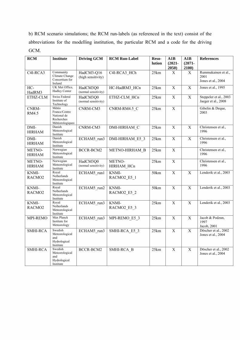
Deliverable 2B.35 Journal papers on the impacts application of methods for the construction of probabilistic regional climate projections At the time of writing (February 2010), four papers are published, or in press, and another three are in preparation. They are referenced below and represent the output from three partners: ULUND, NIHWM and FUB. Another partner, PAS, is expected to publish results of relevance to this deliverable at a later date, and a summary of some of the work they have done using probabilistic projections may be found in the ENSEMBLES final science summary report, downloadable at: http://ensembles-eu.metoffice.com/docs/Ensembles_final_report_Nov09.pdf Papers marked with an asterisk (*) are reproduced in this document. Donat M.G., Leckebusch G.C., Wild S., Ulbrich U., 2010: Future changes of European winter storm losses and extreme wind speeds in multi-model GCM and RCM simulations. Special Issue of Natural Hazards and Earth System Sciences (NHESS): Applying ensemble climate change projections for assessing risks of impacts in Europe, in press. * Jönsson, A.M., Appelberg, G., Harding, S. and Bärring, L. 2009: Spatio-temporal impact of climate change on the activity and voltinism of the spruce bark beetle, Ips typographus Global Change Biology 15:486-499. * Mares C., Mares I., Mihailescu M., Hübener M., Cubasch U., Stanciu P., 2009: 21st century discharge estimation in the Danube lower basin with predictors simulated through EGMAM model. Revue Roumaine de Géophysique, tom 52, 2009. Rammig, A., Jönsson, A.M., Hickler, T., Smith, B., Bärring, L., Sykes, M.T. 2010: Impacts of changing frost regimes on Swedish forests: Incorporating cold hardiness in a regional ecosystem model. Ecological Modelling 303-313. * In preparation: Jönsson, A.M., Harding, S., Krokene, P., Lange, H., Lindelöw, Å., Økland, B. and Schroeder, L.M. Modelling the potential impact of global warming on Ips typographus voltinism and reproductive diapause. Jönsson, A.M., Bärring, L. Ensemble-based analysis of climate impact on Norway spruce bark beetle swarming activity in northern and central Europe. Jönsson, A.M., Bärring, L. Warming up for spring backlashes in Norway spruce forests.

Future changes of European winter storm losses and extreme wind speeds in multi-model GCM and RCM simulations

M.G. Donat, G.C. Leckebusch, S. Wild, U. Ulbrich

Institute for Meteorology, Freie Universität Berlin, Germany

Correspondence to: M. G. Donat (markus.donat@met.fu-berlin.de)

Abstract

Extreme wind speeds and related storm loss potentials in Europe are investigated based on

multi-model simulations with global (GCM) and regional (RCM) climate models. Potential

future changes due to anthropogenic climate change are analysed from simulations according

to the IPCC SRES A1B scenario. The large number of considered simulations allows for an

estimation of the robustness of the identified climate change signals.

All models in general reproduce the observed spatial patterns of wind speeds, although partly

systematic biases are found for some models. A storm loss model is applied to the GCM and

RCM simulations. It is found that the resulting mean loss amounts calculated based on the

20th century climate simulations are realistic, whereas the inter-annual variability of losses is

generally underestimated. For the future scenario, most simulations as well as the ensemble

mean generate enhanced extreme wind speed values (up to 5% in the ensemble mean) over

northern parts of Central and Western Europe. As a consequence, also loss potentials are

increased in these regions, particularly in Central Europe. For Southern Europe decreased

extreme wind speeds and loss potentials are analysed. There is, however, a considerable

spread between the change signals of the individual ensemble members, with signatures

opposite to the ensemble mean signal analysed in some models. The downscaling of the large-

scale simulations with RCMs increases the range of computed change signals. Even RCMs

with identical large-scale driving show partly different change signals. The robustness of the

change signals is estimated by two different measures: First, the inter-model standard

deviation is considered which is, however, sensitive to outliers and thus reveals large

uncertainty ranges. Second, robustness is estimated by means of multi-model combinatorics,

considering all possible sub-ensembles from GCMs and RCMs and hence taking into account

the arbitrariness of model selection for multi-model studies. Based on all available GCM and

RCM simulations, e.g. for Germany an ensemble mean increase of loss potentials by +25% is

analysed for the end of the 21st century, and 90% of the possible results show increased loss

potentials in a range between +15% and +35%.

1 Introduction

Mid-latitude winter storms frequently hit Europe. Barring the risk of injury or even loss of

lives those events cause heavy damages, in particular to infrastructure. The related losses

often amount to several millions of Euros for single events and thus wind storms are the most

loss-intensive natural hazards in Central Europe. For example in Germany 53 percent of

economic losses due to natural hazards and even 64 percent of insured losses are caused by

winter storms (Munich Re, 1999; Munich Re, 2007). It is thus important for different

institutions involved in planning, rescue and insurance to gain information on how the risk of

those extreme events might change under anthropogenic climate change (ACC) conditions.

Considering changes of storminess during the recent past, a high inter-decadal variability

becomes obvious and often no clear trends can be identified during the last century (Bärring

and von Storch, 2004; Matulla et al., 2008). On the other hand, studies focussing on storms

during the winter season presented upward trends towards the end of the 20th century

(Leckebusch et al., 2008a; Wang et al., 2009). Time series of monetary storm losses show

clear upward trends during the recent decades. Barredo (2009) associates this trend, however,

mainly with societal factors, in particular with increasing values. For normalised losses no

clear trend is found. A number of studies have recently dealt with changes of storminess in

ACC scenario simulations using global climate models (GCMs) and found indication for

more frequent occurrence of intensive cyclones over eastern North-Atlantic (Bengtsson et al.,

2006; Lambert and Fyfe 2006, Leckebusch et al., 2006) and an eastward extension of the

North Atlantic storm track (Ulbrich et al., 2008). This is in line with findings of higher

extreme wind speeds over parts of Western and Central Europe (Knippertz et al., 2000,

Leckebusch and Ulbrich, 2004, Pinto et al., 2007; Gastineau and Soden, 2009). Based on

multi-model GCM simulations, Donat et al. (2010a) found increased frequencies of storm

days under future climate conditions as well as increased wind speeds during storm events.

Studies estimating changes of storm losses under ACC conditions found increased risk of

losses particularly in Western and Central Europe if no adaptation of buildings to higher wind

speeds takes place (Leckebusch et al., 2007; Pinto et al., 2007).

Such investigations based on GCMs can be complemented by applying dynamical

downscaling with regional climate models (RCMs). This way, atmospheric information at a

higher spatial resolution is obtained, in particular providing information on the influence of

regional orographic characteristics. Additionally, physical processes acting on scales resolved

by the RCMs (but not by the GCMs) might affect the simulated regional wind patterns. The

profit of dynamical downscaling with respect to wind fields over complex terrain was

demonstrated e.g. by Žagar et al. (2006), obtaining wind speeds in better accordance with

observations for mountainous regions compared to the driving large-scale reanalysis. An

improved representation of local wind speeds should allow for a higher accuracy of storm loss

calculations. The benefit of dynamical downscaling for storm loss calculations was

documented in a recent study using loss data for Germany (Donat et al., 2010b). Future

changes of extreme wind speeds in multi-model RCM simulations (all driven by the same

GCM) have been explored by Rockel and Woth (2007), finding increased speed values in

Central and Western Europe during winter. ACC signals of wind speed patterns in RCM

simulations driven by different GCMs were previously investigated in comparison to the

large-scale GCM signals e.g. by Leckebusch et al. (2006).

It is well known that results from numerical climate model simulations are affected by

different sources of uncertainty. The most important ones are sensitivity to the initial

conditions, to boundary conditions, model uncertainties and uncertainty due to internal

variability. Due to non-linear processes in the climate system, small variations in the initial

conditions of the simulations might lead to different solutions for the simulated state of the

atmosphere. This source is most relevant for shorter time scales like weather and seasonal

prediction applications, while climatological means computed from long-term climate

projections are largely insensitive to small variations in the initial state (cf. Tebaldi and

Knutti, 2007). However, recent studies (Pinto et al., 2007) showed that with respect to ACC

signals of extreme wind speeds over Europe, runs of the same model under the same climate

scenario, but started from different initial conditions, can produce a rather large range of

signals. Further, the climate system features a natural (internal) variability with periods from a

few years up to decades and climate models generally do not reproduce the observed

chronology of events. Thus, a sampling uncertainty is introduced by the fact that model

climate states are estimated from a finite number of years. The occurrence of wind storms is

of particularly high variability (Bärring and von Storch, 2004, Matulla et al., 2008), so for a

reliable estimation of trends large samples are desirable (which can also be produced by

ensemble simulations, see e.g. Della-Marta et al., 2009). Boundary condition uncertainty

includes the different possible future greenhouse gas (GHG) emission scenarios, based on

hypotheses about future developments which include assumptions about possible societal

changes, use of resources, global vs. regional development, etc. (e.g. Nakićenović et al.,

2000). Model uncertainty is due to inaccuracy arising from the computational representation

of the dynamic equations and the different parameterization of sub-grid processes. It is

generally larger than the other sources (Déqué et al., 2007) and thus, results of ACC studies

might be fundamentally dependent on the particular climate models taken into account.

Combining different models to a multi-model ensemble (MME) generally increases the skill,

reliability and consistency of model projections. The superiority of MMEs for weather and

seasonal prediction applications could be widely shown (see e.g. Hagedorn et al., 2005) and a

verification and quantification is relatively straight-forward e.g. by skill measures. Also for

climate-timescale simulations a MME can be favourable compared to a single model (cf.

Palmer and Räisänen, 2002; Räisänen, 2007, Collins, 2007). MMEs primarily sample initial

condition and model uncertainties (Tebaldi and Knutti, 2007) and by increasing the sample of

considered years also the uncertainty due to internal variability should be reduced. Donat et

al. (2010b) demonstrated the profit of MMEs for storm loss calculations, showing the

ensemble mean performance to be close to the best single model and an increased agreement

of the results for the more models are included in the ensemble.

Aim of this study is to estimate a range of possible future changes of extreme wind speeds

and related storm loss potentials, as well as the robustness of the change signals based on a

multi-model ensemble of GCM and RCM simulations. Further, the change signals in the

RCMs are compared to the signals in the driving GCM. The robustness of the change signals

can be estimated based on the differences between the signals from the different ensemble

members. The availability of a large ensemble of (GCM and RCM) simulations conduces to

an estimation of a possible range of change signals as well as of the signal (un-) certainties.

We follow two different approaches for estimating this uncertainty: In addition to considering

the inter-model standard deviation, the effect of different ensemble configurations on the loss

signals is examined systematically for all possible combinations of subsets of available

models. This allows for giving probabilistic information about the magnitude of possible

changes.

This work is part of the ENSEMBLES project (http://ensembles-eu.metoffice.com/index.html,

cf. Hewitt, 2005), where multi-model simulations with state-of-the-art global and regional

climate models are produced and investigated with respect to the assessment of uncertainties

in future climate projections.

2 Data and Methods

2.1 Meteorological Data

In total, 9 GCM simulations from 6 different GCMs are considered (ENSEMBLES project

setup, see table 1a). From each simulation, a period representing recent greenhouse gas

forcing conditions during the last decades of the 20th century (20C) and a projection of future

climate for the 21st century (21C) according to the SRES A1B scenario (A1B) are analysed.

Two future periods are regarded: one for the middle (2021-2050) and one for the end of 21C

(2071-2100 of most models).

All RCM simulations were carried out for a common domain including the whole continental

European area (from approximately 10°W to 40°E and 30°N to 65°N). Overall, a set of 14

RCM simulations was considered (table 1b), downscaling 7 different GCM runs. Most of

them are carried out at a resolution of 0.22° (approximately 25km), 2 simulations (KNMI-

RACMO2_E5_1/2; for an explanation of the nomenclature of the RCM run-labels please cf.

table 1b) were performed in a coarser resolution of 0.44° (approximately 50km). All scenario

simulations follow the SRES A1B scenario and are integrated until at least year 2050. A

smaller set of simulations continues until year 2100. Thus, we examine climate change signals

for the middle (of all models) as well as for the end (of the subset of models integrating until

2100) of the 21st century. For the 4 HadCM3-driven simulations (C4I-RCA3_HCh, HC-

HadRM3_HCn, ETHZ-CLM_HCn and METNO-HIRHAM_HCn) different realisations from

a perturbed parameter GCM-ensemble have been used for boundary forcing. Due to their

different sensitivities (detailed description in Collins et al., 2009) they must be considered as

simulations with different models. Unfortunately no daily maximum wind speeds were

available from these HadCM3 runs that would allow for an interpretation of the RCM signals

in context with the large-scale forcing. This is, however, possible for the remaining 10 RCM

simulations, driven by GCMs also analysed in this study (cf. section 3.1): each 2 driven by

CNRM-CM3 and BCCR-BCM2, in total 4 driven by MPI-ECHAM5_run3 and each 1 driven

by MPI-ECHAM5 run 1 and 2, respectively (cf. table 1b).

The investigated ensemble of GCM simulations is obviously dominated by the ECHAM5

model (in total 4 of the 9 simulations are based on this model), and the presented results could

thus potentially be biased due to the dominance of this particular model. As we prefer to

include as many simulations as possible in our ensemble, we generally considered all 9

available simulations to compute the GCM ensemble mean. This approach also seems to be

reasonable as the change signals from the individual realisations with ECHAM5 reveal a

considerable spread. Nevertheless, the results will also be discussed for the case that only one

of the ECHAM5 simulations contributes to the ensemble. Similarly, the RCM ensemble

consists of different models downscaling the same GCM simulation. As even RCMs with

identical large-scale forcing reveal considerably different results (cf. section 3.2) and given

the aim of this study to incorporate as many models as available, generally all simulations are

included in the ensemble mean calculations. Nevertheless, the impacts of alternative ensemble

constructions will be discussed.

ERA40-reanalysis (Uppala et al., 2005) is used for validation of the GCM and RCM 20C

climate period simulations. Further, these data are used for calibration of the loss model; the

obtained loss regression function is also used for loss calculations based on the GCM

simulations (see methods section 2.2).

Our analyses concentrate on the daily maximum 10-m wind speeds from all data sets. This

parameter is recorded as the daily maximum speed value, based on all time steps within a 24 h

period. It was derived for almost all GCMs and for all RCMs. Only 6-hourly instantaneous

values of wind speed were available for ERA40 and the GCM simulations with BCCR-

BCM2, CNRM-CM3 and DMI-ECHAM5. Hence, a daily maximum is calculated as the

maximum of the 4 instantaneous wind speeds stored at 00, 06, 12 and 18 UTC. This value is

expected to be slightly smaller than the maximum over all time steps (cf. Pinto et al., 2007,

their figure 3b,c), inducing a small inhomogeneity to our data basis. The daily maximum wind

speed data are hereafter referred to as WIMAX.

Five of the RCMs (used for in total 8 simulations) also feature a gust parameterisation: C4I-

RCA3_HCh, ETHZ-CLM_HCn, SMHI-RCA_B, MPI-REMO_E5_3, KNMI-

RACMO2_E5_1,2,3 and SMHI-RCA_E5_3. The respective daily maximum 10-m gust wind

speeds are hereafter referred to as GUST. For the ERA40 dataset the 10-m wind speed (6-

hourly, see above) and a 10-m wind gust is available. As in the RCMs, the latter is a model

diagnostic and hence calculated based on a parameterization. Note that different approaches

for calculating the gust wind speeds are used in the different models. The method used in the

RCA models (SMHI and C4I) assumes that surface gusts result from the deflection of air

parcels from the upper boundary layer, mixed down by turbulent eddies (Brasseur, 2001).

This method takes into account turbulent kinetic energy, the mean wind and the static stability

in the boundary layer. ERA40 and KNMI-RACMO2 make use of a scheme based on the

similarity relation by Panofsky et al. (1977). Here, a standard deviation of the near-surface

wind is calculated, again taking into account the static stability of the boundary layer. The

maximum gust speed in than estimated by adding a term including this standard deviation to

the 10m wind speed (cf. White et al., 2003). MPI-REMO and ETHZ-CLM calculate gusts

based on empirical assumptions taking into account the turbulent kinetic energy in the lowest

model layer (Schrodin, 1995).

Almost all severe damage causing storm events occur during boreal winter (Klawa and

Ulbrich, 2003; Munich Re, 2007). Hence, the analyses presented here focus on the extended

winter period October to March.

2.2 Calculation of storm induced losses

Storm losses are calculated by applying a linear regression model developed by Klawa and

Ulbrich (2003). In recent studies this model was applied to reanalysis and GCM data

(Leckebusch et al., 2007, Pinto et al., 2007) as well as to (reanalysis-driven) RCM simulations

(Donat et al., 2010b), revealing reasonable results. Annual loss ratios (giving the ratio of

insured values that is affected by storm losses) are calculated by the equation

BLLIareapopAlossGermany

area

Jahr

Tage+= ∑ ∑*)(*

with local loss index 3

98

max 1)(

),(⎟⎟⎠

⎞⎜⎜⎝

⎛−=

areavdayareav

LLI (for , else LLI=0) 98max vv >

In this function is the daily maximum wind speed (i.e. WIMAX or GUST) in a grid box and

is the local 98th percentile of daily maximum wind speeds. Thus, it is assumed that losses

occur locally during the 2% of days with strongest winds. Using a relative threshold, the loss

function takes into account model biases of simulated wind speeds. A is the obtained

regression coefficient from calibrating calculated losses with the insurance data and B is the

axis intercept; pop(area) is the population density. Population density is regarded as a proxy

for insured values, because information about spatial distribution of total insured values are

highly sensitive for insurance companies and thus difficult to assess. Particularly for Central

and Western Europe the assumption is reasonable that insured values are proportional to

population density. For the calculations in this study we use gridded population density data

for the year 2000, on a 0.25x0.25 degree raster (CIESIN 2005).

The loss index (calculated at each grid point) has to be calibrated with loss data from

historical storms. Therefore, annually accumulated loss data (including losses to residential

buildings due to storm and hail events) for Germany were provided by the Gesamtverband der

Deutschen Versicherungswirtschaft e.V. (German Insurance Association, hereafter GDV) for

the period 1970-2000. The large losses are usually caused by intense winter storm events

affecting a large area; losses due to hail can generally be neglected, as their percentage in the

total annual loss is small (Klawa and Ulbrich, 2003; pers comm. GDV, 2009). Annual loss

values are given as loss ratios, i.e. the ratio between insured claims and totally insured values

(unit: € per 1000€, i.e. in ‰). An advantage of this measure is that inflation can be neglected

as it is included in both, in insured values and in the loss. A linear regression is used to

calibrate “raw losses” as calculated by the loss function with the GDV loss ratios. We used

the regression derived for Germany also for the other considered countries. Leckebusch et al.

(2007) showed that similar results are obtained if damage data from the UK were used to

calibrate the calculated loss values. Thus, the calculated loss ratios for other countries than

Germany might not be fully realistic in terms of their absolute value, but estimates of future

changes will still be possible. Besides for Germany, in this study storm losses are estimated

for Poland, France, Belgium, Netherlands and Luxembourg (together “BeNeLux”), United

Kingdom and Ireland (together “UK+IRE”) and Spain and Portugal (together “IBERIA”).

This selection is motivated by former results with respect to future changes of loss potentials

and cyclone tracks (e.g. Leckebusch et al., 2006; 2007; Donat et al., 2010a) Population

densities used for the loss calculations for these considered regions are presented in figure 1.

For the calculation of losses from the GCM simulations the regression of “raw losses” and

insurance data determined for losses calculated from the ERA40-reanalysis is used. Because

the models simulate a specific realisation of climate and generally do not reproduce the

observed chronology of events, model years can not be assigned to observed annual loss data.

GCM wind biases against ERA40 are less relevant, as normalised wind speeds rather than

absolute model output values are used. For the RCM simulations model-specific regressions

were determined from simulations driven by ERA40-reanalysis, which are expected to depict

the observed chronology of storm events and related losses (cf. Donat et al., 2010b). Again,

deviations of a RCM wind climatology arising from driving the model with GCM data other

than ERA40 are largely removed by the percentile approach.

Loss potentials for the future climate periods are calculated in two ways: in the first, the local

98th percentile of daily maximum wind speeds calculated for the 20C period is maintained as

the threshold for the occurrence of losses also for the future climate simulations; in the second

approach the percentile of the future simulation is used as the loss threshold. The first

approach means that damage should occur at the same wind speed as presently. Thus, damage

to buildings occurs without adaptation to a new wind climatology. The second approach takes

adaptation into account. This means that e.g. the architecture of houses is adapted to higher or

lower local wind speeds, so that losses again occur only during the 2% of days with highest

wind speeds (also refer to Leckebusch et al., 2007; Pinto et al., 2007)

3 Extreme wind speeds and related losses estimated from GCM and RCM scenario simulations

3.1 Analysis of the GCM simulations

3.1.1 Extreme wind speeds

Regarding the ensemble average of all GCMs, there is a general agreement with the ERA40

reanalysis for both spatial patterns and absolute speed values (figure 3a/b), although

peculiarities are found in some individual models. The GCM ensemble reveals systematically

higher speed values in comparison to ERA40 over the Atlantic and the Mediterranean

(approximately 5%), whereas over land and parts of the Baltic region lower speed values are

found (up to 10%). Still, the typical patterns of extreme wind speeds (here: 98th percentile of

WIMAX) in the European region with maximum values over sea areas and lower values over

continental areas are also reproduced by all GCMs (figure 2a). Over land areas, highest wind

speeds are found over northern parts of Western (British Isles, northern France) and Central

Europe (Benelux, Denmark, northern Germany and northern Poland) and also over parts of

Scandinavia. Minimum speed values are over terrain with complex orography. FUB-EGMAM

reveals relatively high speed values also in the area of the Iberian Peninsula. Note that this is

the model with the coarsest spatial resolution and uses sea grid boxes in this area to keep the

Strait of Gibraltar opened. Thus, lower roughness allows for higher near-surface wind speeds,

disagreeing with the observation-based (reanalysis) data set.

Although the speed values in the individual models are in a similar scale, there are some

specific differences. For example, wind speeds in FUB-EGMAM are systematically higher

compared to ERA40 and the other models, while IPSL-CM4 and CNRM-CM3 reveal largely

lower speed values. These differences can only partly be assigned to the different calculation

of daily maxima. Remember that for some models daily maxima were calculated as maxima

of 6-hourly instantaneous values (ERA40, CNRM-CM3, BCCR-BCM2, DMI-ECHAM5, cf.

Section 2). The model-to-model differences of absolute wind speeds can be largely resolved

by the use of relative thresholds for loss calculations in subsequent parts of this paper.

The ensemble mean A1B scenario signal for the end of the 21st century (figure 3b) features a

significant increase of extreme wind speeds over northern parts of Central and Eastern Europe

and a decrease over the Mediterranean. Similar results are found in most of the individual

GCMs (figure 2b), whereas the exact position of the maximum change is shifted somewhat

east- or westwards in the individual ensemble members. The most different signal is found in

the IPSL-CM4 simulation: here, the zone of significantly increased wind speeds is shifted

north-eastwards towards the northern Baltic region, whereas over Western Europe a decrease

of extreme wind speeds is analysed. A decrease over Western Europe is similarly found in the

HadGEM1 simulation. At the same time, this simulation also reveals a particularly strong

increase of the 98th percentile of daily maximum wind speeds over Eastern Europe, up to

nearly a doubling. The third run of MPI-ECHAM5 produces the smallest signal of all

simulations; in particular the increase of extreme wind speed over Central Europe is not

significant in this realisation.

The characteristics of the ACC signals for the first half of the 21st century are similar as those

for the end of the 21st century in all individual models, though magnitude and significance are

mostly lower (not shown). In the ensemble mean there is even a small (non-significant)

decrease over the North Sea region for this early period which is mainly caused by the signals

from IPSL and HadGEM1.

3.1.2 Loss potentials

Insurance companies have to pay on average about 900 million € per year only in Germany as

a consequence of storm losses to residential buildings (GDV 2006; 2009). On the basis of the

German insurance data, for the recent decades a mean annual loss ratio of approximately

0.15‰ (±0.12‰ inter-annual standard deviation) is assumed (compare also Leckebusch et al.,

2007; Pinto et al., 2007; Donat et al., 2010b). Despite model-specific differences in the wind

climatologies and also specific decadal variabilities, realistic annual mean losses are

simulated on the basis of output from the 20C runs (cf. table 2), supporting the applicability of

the GCMs for loss estimates. From the simulations with ECHAM5 and HadGEM1, mean loss

ratios are closest to the insurance data (between 0.14 and 0.16‰); somewhat lower values are

obtained from the other models (e.g. 0.11‰ from CNRM-CM3). The inter-annual standard

deviation of annual losses is too low in all models except for DMI-ECHAM5. Based on this

model, the mean loss ratio as well as the standard deviation is closest to the insurance data.

Losses calculated from the other models reveal a too low inter-annual variability compared to

the observed insurance loss data.

Examining the storm losses in the ACC simulations for the end of the 21st century,

considerable differences between the individual ensemble members are apparent, particularly

for the case of no adaptation (Appendix table AT1a). Considering area averages for individual

countries, largest changes are found for Germany, with 8 out of 9 ensemble members showing

enhanced risk of mean loss, up to +87.1% (HadGEM1). Only losses calculated from the DMI-

ECHAM5 simulation show slightly decreased values (-6.2%). In the ensemble average (figure

4, upper row), the annual mean loss ratio for Germany is increased by 37.7 (±31.0)%. This

increase goes along with an increased standard deviation of the annual losses in 7 of the 9

simulations and also in the ensemble mean. The increase of inter-annual variability is

primarily caused by the occurrence of individual years with extremely high losses, partly

occurring during single exceptionally strong events (Leckebusch et al., 2008a), which do not

occur in the GCM control periods. Thus, the increase of the inter-annual standard deviation

might be even more relevant for impact assessments than changes in mean losses.

In the future climate simulations, France is affected by higher extreme wind speeds in its

northern parts and lower extreme wind speeds in the Mediterranean region (cf. figure 3b),

partly compensating each other in the country mean. Consequently the change signals for

France are relatively small. In the average of all simulations risk is increased by 9.0 (±13.2)%,

with slightly increased inter-annual variability (measured in terms of standard deviation of

annual loss values). 7 out of the 9 ensemble members reveal increased risk by up to +36.5%

(FUB-EGMAM), and in 2 ensemble members storm losses are slightly decreased (up to -

7.6% in HadGEM1).

For the BeNeLux area 7 of the 9 ensemble members reveal increased loss potential of up to

+50,4% (CNRM-CM3) and in the other 2 GCM simulations a slightly decrease of about -4%

is analysed. The ensemble mean indicates increased values of mean annual losses by +17.6

(±21.2) %. Also the inter-annual variability of loss is significantly increased in this area.

Cumulated losses of the United Kingdom and Ireland increase in 7 of the 9 ensemble

members (up to 67.6% in FUB-EGMAM). The 2 models revealing reduced extreme wind

speeds over Western Europe (cf. Fig. 2b) also feature considerably lower loss values

(HadGEM1: -22.1%, IPSL-CM4: -16.5%). In the ensemble average, mean annual losses are

enhanced by +17.4 (±32.3) %. Also the standard deviation of annual losses is considerably

enhanced (+27.8% in ensemble mean), although only 5 ensemble members feature increased

inter-annual variability, in the other 4 it is reduced.

For the Iberian Peninsula (where reduced extreme wind speeds were analysed) 7 ensemble

members reveal also decreased losses (HadGEM1 up to -24.2%). In 2 ensemble members a

light increase is found (BCCR up to +8.4%). The ensemble average of mean annual losses is

reduced by -10.1 (±10.0) % in this area.

A significant increase of extreme wind speed values was found over eastern Central Europe in

the ACC simulations (Fig 3b). Regarding now the change signals of loss potentials in Poland,

the majority of 7 ensemble members features enhanced risk of loss (HadGEM1 up to

+52.8%); 2 realisations feature small decreases (MPI-ECHAM5 run1 up to -7.6%).

Consequently, in ensemble mean an increase of mean annual losses by +12.1 (±18.3)% is

found.

The 4 simulations with the ECHAM5 model reveal considerably different loss changes (cf.

table A-1a). Although comparing the individual ECHAM5 signals with the other models does

not suggest any suspect that the ensemble results could be biased due to including multiple

runs of this particular model, we recalculated the ensemble mean loss changes including only

1 simulation of each GCM. Thus, 4 different ensembles of 6 different GCMs can be

constructed (each containing either realisation 1, 2 or 3 of MPI-ECHAM5 or the DMI-

ECHAM5 run). Indeed, considering only 1 of these simulations for the ensemble mean

calculation, the presented results remain largely valid, though there are some modifications

with respect to the ensemble mean signals’ magnitudes. For example, the modified ensemble

mean change signals for losses in Germany range between +41.4 % (including the DMI run)

and +51.2 % (including MPI run1). For UK and Ireland increased losses between 14.3 %

(including MPI run2) and 23.2 % (including MPI run1) are found; or e.g. for the BeNeLux

region the different ensemble mean signals range between +14.9 % (including MPI run3) and

+22.3 % (including MPI run1). Thus, the large spread of possible signals between the

different realisations of this particular model, comparable to the spread of signals based on the

different GCMs, justifies the inclusion of all available simulations. We find no evidence for a

bias due to including different realisations of the same model. Hence, including all

simulations enlarges the ensemble size and allows for a sound estimation of the change

signal’s robustness.

Future loss calculations for the case that adaptation takes place (i.e. the threshold for

occurrence of losses is adapted to future wind climate so that at each grid point again the 2%

strongest wind events cause losses) reveal distinctly smaller changes (Appendix table AT1b).

For example for Germany, the spread of changes in the different ensemble members is

between +16.8% (IPSL-CM4) and -22.6% (DMI-ECHAM5). In ensemble mean, change

signals for Germany, France, BeNeLux and UK with Ireland are small (up to 2%), though

increased inter-annual variability of losses is still found for Germany. For the Iberian

Peninsula and Poland changes of mean losses are about 6.5% increase (IBERIA) or decrease

(Poland), respectively. Increased losses for the Iberian Peninsula are also found in 8 of the 9

ensemble members. Please note that due to the reduction of extreme wind speed in this region

also the threshold for loss is reduced. Thus, the adaptation approach would correspond to an

adaptation to weaker structures of buildings here.

Change signals for the first half of the 21st century (considered 2021-2050) mostly show the

same characteristics as the signals for the end for the 21s century (upper row in figure 4b for

loss changes without adaptation), but largely a lower magnitude, although still a large

variability between the ensemble members is apparent (Appendix table A-1c). In ensemble

mean the magnitude of changes for Germany in the middle of the 21st century is about 50%

compared to the change signal at the end of the 21st century. For France and Poland the

difference between the two forcing periods is small; for United Kingdom and Ireland the

mean signal is about 33%, for the Iberian Peninsula 50% and for BeNeLux 40% of the mean

signal for the end of the 21st century. Regarding the ratio of change signals between the

earlier and the later future climate period in the individual ensemble members discloses a

large variability between the different realisations. Whereas in some cases even contrary

signals are found for the two periods (e.g. for Germany: IPSL-CM4, DMI-ECHAM5, MPI-

ECHAM5_run3; for France: FUB-EGMAM, HadGEM1, MPI-ECHAM5_run2; for Poland:

MPI-ECHAM5_run1), also examples with double or even higher magnitude of change in the

earlier period can be found.

These results demonstrate the high variability on a decadal scale in the occurrence of severe

wind storms in the different realisations. The analysed loss potential change signals partly do

not seem to scale proportional with the GHG forcing, as the identified signals include both,

internal variability and response to ACC. In the ensemble mean the pattern of the change

signals is comparable for both future periods, demonstrating the value of an ensemble by

enlarging the sample size and thus reducing the uncertainty due to internal variability. In the

case of adaptation of the loss threshold to the changed wind climate again only small changes

are found (not shown).

3.2 Analysis of the RCM scenario simulation

3.2.1 Extreme wind speeds

Patterns of the 98th percentile of WIMAX as produced by the GCM-driven RCM simulations

for the 20C period do not show major deviations from the reanalysis-driven runs (figure 5a,

compare to Donat et al., 2010b). The model-specific characteristics (such as systematic biases

in absolute speed values and anomalies over mountainous regions) discussed in the previous

study for the ERA40-driven simulations are almost identical with those originating from the

(GCM-driven) 20C scenario simulations.

For the RCM future scenario simulations (figures 5b and figure 6a,b), significantly increased

extreme wind speeds are found in the ensemble mean particularly over Western Europe and in

the North Sea and Baltic Sea regions; over the Mediterranean reduced wind speeds are

analysed. These are common features also in the majority of the RCMs. The C4I-RCA3_HCh

simulation (driven by HadCM3-Q16, i.e. high sensitivity) is the only one showing largely

decreased wind speed values also in the Central European region. Whereas relatively smooth

signals are found in the GCM simulations (cf. section 3.1), the signals in most individual

RCMs noticeably appear somewhat spotty over continental areas. Consequently they partly

seem to compensate in the ensemble mean and thus, the changes over Central Europe are

comparatively lower than in most of the individual models and also than in the GCM

ensemble. Although patterns of the change signals are similar when driven by the same GCM,

with respect to the signals’ magnitudes a considerable spread becomes obvious. Note e.g. the

differences between the 4 simulations driven by ECHAM5_run3 and also remember that the

driving run reveals only marginal change signals (cf. figure 2b).

The ensemble mean patterns of the change signals for the middle of the 21st century (figure

6a) correspond again well to the patterns for the end of 21C (figure 6b), whereas the

significance of the signals is considerably higher for the later period. Please note that in the

ensemble for the earlier period there are 3 more simulations included than in the ensemble

mean for the end of 21C, because CNRM-RM4.5_C, METNO-HIRHAM_B and METNO-

HIRHAM_HCn were only integrated until 2050. The picture is, however, similar if the

ensemble mean for the earlier period is calculated only from the 11 simulations which are also

available for the later period. Also regarding the individual ensemble members, for those

simulations integrated until 2100 generally the decrease over Mediterranean is more

significant for the latter period. Particularly the DMI-HIRHAM_E5_3 and KNMI-

RACMO2_E5_1/2/3 simulations reveal a considerably stronger increase over Western and

Central Europe for the later period, whereas for the other simulations signals in this region are

similar for both periods.

3.2.2 Loss potentials calculated from the RCM simulations

Regarding the RCM storm loss potentials, the change signals correspond in general to the

signals found from the GCM simulations, although for most regions the mean relative

changes are slightly smaller in the RCM ensemble (figure 4, bottom row, compare with top

row). Again there are considerable differences between the individual ensemble members

(Appendix table AT2). In the following paragraph the ensemble mean changes (± standard

deviation between the different simulations) and additionally the maximum spread (i.e. the

most extreme signals) are discussed.

Following the no-adaptation approach, storm losses in Germany could increase by +15.1

(±17.1) % in ensemble mean for the end of 21C (spread between +54.9 % (KNMI-

RACMO2_E5_3) and -4.5 % (SMHI-RCA_E5_3)). For France, the ensemble mean change

signal is +5.8 (±7.4) %, for UK together with Ireland +18.5 (±18.6) %, for BeNeLux +8.0

(±11.4) %, for Poland +6.1 (±9.9) % and for the Iberian Peninsula by -4.2 (±5.6) % decreased

losses are analysed. Again a noticeable increase of inter-annual variability of losses is

diagnosed, particularly for Germany, Poland, BeNeLux and UK+IRE.

Analysis of different RCMs driven by the same GCM simulation reveals that despite identical

large-scale driving, dynamical downscaling might increase the spread of possible results

considerably. Regarding e.g. the 4 RCM simulations driven by ECHAM5_run3, change

signals between +33.6% and -4.5% are obtained, whereas the change signal of the driving

ECHAM5_run3 is +17.0%: 1 RCM simulation reveals a considerably stronger change signal

(KNMI-RACMO2_E5_3), 2 realisations (MPI-REMO_E5_3 and SMHI-RCA_E5_3) show

only small changes of loss, and in the DMI-HIRHAM-E5_3 run the change signal is almost

identical with the GCM signal. Thus, with respect to the large spread, the average signal of

the 4 RCM runs is similar (+12.4%) to the GCM signal, but still about 30% too low. Further

analysis of the impact of regional downscaling related to the spread of climate change signals

seems thus to be motivated and of additional need, but is behind the scope of this study.

Note that the magnitude of mean change signals in the RCM ensemble is for all regions

except for UK and Ireland considerably smaller compared to the signal’s magnitude in the

GCM ensemble. This might partly be explained by the model setup, as e.g. the GCM

simulations showing the largest change signals were not used to drive RCM simulations (cf.

tables 1a,c and section 2). Further, 4 RCM scenario simulations were driven by different

perturbed-parameter experiments with the HadCM3 model; daily maximum wind speeds from

these experiments were not available for this study and could thus not be included in the

GCM ensemble. Nevertheless, the phenomenon of comparatively smaller signals in the RCM

ensemble is still present if only those GCM simulations that were used for downscaling are

considered in the GCM ensemble mean and only those RCM simulations where the driving

GCM simulation is available are considered in the RCM ensemble. However, in some cases

(e.g. KNMI_RACMO2_E5_3) also stronger RCM signals are found in comparison to the

driving GCM. Understanding the differences between the signals from the large-scale and

regional models makes further studies necessary.

Ensemble mean change signals for the first half of 21C (figure 4b, bottom row) are small

(below 5%) for most of the considered regions, only for UK+IRE a considerable signal is

found (+12.5 (±14.3) %). As already found for the GCM simulations, change signals are small

in the case that adaptation of the loss threshold to the future climate is taken into account (not

shown), demonstrating the value of in time initiation of adaptation strategies.

3.2.3 Does the use of RCM gust wind speeds modify the results?

From a subset of the RCM simulations also gust wind speeds estimations (as a model

diagnostic) are available. The heavy damages in the “real world” are generally caused by

severe wind gusts; Rockel and Woth (2007) documented that wind speeds exceeding 20m/s

(8Bft.) are in general not produced by RCMs without a gust parameterisation. However, as

the loss model applied here uses a relative threshold for the occurrence of losses, exceedance

of a specific absolute wind speed should not be necessary for a realistic calculation of losses,

assuming a correspondence of extreme sustained winds and gusts. With respect to the

reproduction of observed losses, Donat et al. (2010b) demonstrated that the temporal

correlation of losses calculated based on GUST is generally not higher than for losses

calculated based on WIMAX.

Also regarding the change signals of extreme wind speeds and loss potentials, the results

presented in the sections above remain largely valid when considering GUST. The patterns of

the ACC signals for the 98th percentile of GUST correspond well to the change patterns for

WIMAX, whereas the change magnitudes and significance levels tend to be stronger for some

simulations (C4I-RCA3_HCh, ETHZ-CLM_HCn and SMHI-RCA_B, not shown) when

regarding GUST. For the other 5 simulations providing GUST (KNMI-RACMO2_E5_1,2,3,

MPI-REMO_E5_3 and SMHI-RCA_E5_3) the change patterns and magnitudes for GUST are

very similar to WIMAX.

Also considering the losses calculated based on GUST, the changes of loss potentials are in

general comparable to loss changes calculated based on WIMAX. Again, C4I-RCA3_HCh

and ETHZ-CLM_HCn reveal somewhat larger signals for most regions compared to

WIMAX, whereas the signals of the other simulations are mostly similar to (or partly even

slightly smaller than) the corresponding WIMAX signals. It is remarkable that for MPI-

REMO_E5_3 the loss changes based on GUST are for all regions almost equal to the results

based on WIMAX. For all regions except for IBERIA this was also found for the SMHI-

RCA_E5_3 run. The ensemble mean loss changes are for most regions comparable to the

RCM mean signals based on WIMAX (compare figure 4). Non-negligible deviations are,

however, found for France and IBERIA. For France, the mean loss change for the end of 21C

is approximately twice (+10.4%) compared to the RCM signal based on WIMAX. For

IBERIA the decrease is by factor 4 smaller (-0.9%).

In summary, we find no systematically altered results if losses are calculated on the basis of

wind gusts instead of WIMAX.

3.3 Multi-model combinatorics: Uncertainty of ACC loss potentials considering all possible model combinations

MME studies are affected by a certain level of arbitrariness. The construction of an ensemble

is for exampled determined by the availability of model simulations. As the individual

simulations produce ACC signals with different magnitudes and even different sign (cf.

chapters 3.1 and 3.2), the MME change signals will depend on the models included. Here, the

influence of different model combinations on the loss potential change signal is for the first

time investigated systematically by considering all possible model combinations in a multi-

model combinatorics approach. The range of the resulting ACC signals allows for an

estimation of the signal’s (un-) certainty. The idea of this approach is to use all information

that are included in the MME. For this study, the composition of the MME was defined by the

models included in the ENSEMBLES project (tables 1a/b).

Based on the 9 available GCM simulations, there are in total 511 different possibilities of

calculating (sub-) ensembles including 1 up to 9 individual ensemble members (9 single

models, 36 combinations with each 2 and 7 models, 84 combinations considering 3 or 6

models, 126 considering each 4 or 5 models, 9 combinations of 8 models and exactly 1

ensemble containing all 9 simulations). Additionally, 14 RCM scenario simulations are

available until 2050 (and 11 until 2100), allowing for 16,383 (or respectively 2,047) different

RCM combinations. Thus, in total 23 individual (GCM or RCM) ACC signals for the first

half of 21C and 20 for the end of 21C are available, enabling 8,388,607 different model

combinations for the earlier period and 1,048,575 for the latter. The consideration all different

possible model combinations can be seen as an “ensemble of (sub-) ensembles”. In basic, this

idea of assessing the uncertainty of the ACC signals is related to the principle of

bootstrapping (Efron, 1979), which is applied to gain information about characteristics (e.g.

quantiles) of an unknown theoretical distribution. However, whereas bootstrapping generally

considers different limited samples to assess the characteristic of a basic population, the

approach presented here accounts for all possible solutions that can be constructed from the

ensemble of models. A limitation might arise from the fact that the different (sub-) ensembles

are not necessarily independent from each other. On the one hand, signals from each

simulation are included in several (sub-) ensembles and on the other hand some of the GCM

simulations are used for driving the RCM simulations (and are thus included in the RCM

results). Further, even different models are not completely independent, as they partly share

common components or modules. This all contributes to difficulties in a sound estimation e.g.

of the degrees of freedom of the sample of possible change signals. Nevertheless, these all are

possible results if only different subsets of simulations were available for this study and thus

have to be included into the considerations. Further, even different realisations with the same

model reveal different change signals (cf. section 3.1) and the RCMs have been shown to

increase the spread of possible results and reveal partly fundamentally different results, even

compared to their driving GCMs (cf. section 3.2). Still, following the suggested approach, a

complete sample based on the different sub-ensembles is gained, making use of all

information included in the ensemble of models. Assuming that the sample of signals

constructed from the available models that are included in the study is representative for a

sample based on all existing climate models, this methodology allows for an estimation of a

range of ACC signals that might be expected.

We focus on the ACC signals without adaptation of the loss threshold (cf. Appendix tables

AT1, AT2). The range of possible change signals on the basis of the GCM and RCM

simulations for the end of 21C is presented in figure 7 for the different regions. The signals of

the different sub-ensembles were counted for different ACC signal magnitudes (in 2%-steps)

and the relative frequency of the different magnitudes is displayed. Here, the green curve

summarizes the results of the 511 GCM combinations (of 9 GCM simulations), the blue curve

represents the 2,047 RCM sub-ensembles (of 11 RCM simulations integrated until 2100), and

the red curve comprises the results from the 1,048,575 combinations of all available GCM or

RCM simulations. For each region, the red shaded area indicates a confidence interval where

the inner 90% of the signals between the 5th and the 95th percentile are found. As each

individual simulation is included in the same number of model combinations, the average of

the ensemble of possible (sub-) ensembles is exactly the same value as for the simple

ensemble mean of all available models (compare also figure 4).

It becomes obvious that the largest spread of ACC signals is found for Germany and the

UK+IRE region. For Germany, the red curve comprising all combinations of available

simulations indicates a mean increase of loss potential of about 25.2%, with the confidence

interval of 90% of the possible solutions between +15.1% and +35.4%. Regarding again all

possible combinations of the GCM and RCM scenario simulations for UK+IRE, loss

potentials for the end of 21C show an increase of 18.1%, with 90% of the possible signals

between +8.4% (5th percentile) and +27.6% (95th percentile). Accordingly, for the BeNeLux

countries a mean increase of 12.3% (confidence interval between 5.7% and 18.8%) is

analysed and for Poland an increase of 8.8% (confidence interval between 3.4% and 14.2%).

The sharpest ranges of possible signals are found for France and the Iberian Peninsula. For

France, a mean increase of 7.2 (±3.9)% is found, and for IBERIA decreased risk of loss by 6,9

(±3.2)%. As already discussed in section 3.2, for most regions (except for UK+IRE) the

magnitude of the signals on the basis of the GCM ensemble (green curves in figure 7) is

larger than the RCM ensemble signal (blue curve). Furthermore, generally also the GCM

spread is larger compared to the spread of RCM simulations, resulting in a broader

distribution of possible results. Remember, though, that those GCMs revealing outlier signals

(and thus contributing to a large spread) were not used to drive RCMs. The phenomenon that

the mean magnitude of change signals for the GCM simulations is considerably larger than

for the RCM simulations is not only found when all available models are considered. If the

ensembles are restricted to those GCMs used for downscaling (and available for this study:

CNRM-CM3, BCCR-BCM2, ECHAM5) in comparison to the connected RCM runs, different

magnitudes are still obvious for the (reduced) GCM- and RCM-ensembles (not shown). The

uncertainty range of the GCM signals is, however, considerably reduced (and similar to the

RCM range) if only those GCMs used for driving the RCMs are considered.

The uncertainty range estimated from all model combinations is considerably smaller

compared to the inter-model standard deviation (compare figure 4), which is more affected by

outlier models. For example, considering only the change signals from the GCM simulations

and the respective confidence interval from the range covering 90% of all 511 possible

results, the mean change signal for Germany is 37.7 (±19.7)%. For comparison, using the

inter-model standard deviation as uncertainty measure (cf. section 3.1.2), the signal was 37.7

(±31.0)%. Accordingly, also for the other regions sharpened confidence intervals are

obtained: mean GCM signal for BeNeLux is +17.6 (±14.4)%, for France +9.0 (±8.1)%, for

Poland +12.1 (±11.5)%, for UK+IRE +14.4 (±21.6)% and for IBERIA -10.1 (±6.3)%.

Mean change signals for the period 2021 to 2050 are generally smaller compared to signals

for the end of 21C (Appendix figure AF1, in accordance with tables AT1c, AT2b). For this

earlier period, considering the 8,388,607 possible model combinations of all 23 ACC

simulations, the widest spreads are again found for Germany and UK+IRE, whereas the

change signals for France and IBERIA reveal the sharpest distributions. The magnitudes of

the mean change signals for this earlier period constitute between 40% (Germany, BeNeLux)

and 70% (France, Poland) compared to the signals for the end of 21C.

4 Summary, Discussion and Conclusion

Patterns of extreme wind speeds and related loss potentials due to severe wind storms are

investigated based on multi-model simulations with global and regional climate models.

Potential future changes are analysed for different European regions according to the IPCC

SRES A1B emission scenario. The considered GCMs and RCMs reproduce well the typical

spatial patterns of extreme wind speeds (98th percentile) over the European region in the

simulations of recent climate, even though some of the models reveal biases in the absolute

speed values. Considering loss potential calculations based on the 20C simulations, realistic

mean losses are obtained; the inter-annual variability of simulated losses is in ensemble mean

about 30% lower than that of observed insurance loss data for Germany. In the future climate

simulations most models and also the ensemble mean commonly feature an increase of

extreme wind speeds over northern Central Europe and a decrease over the Mediterranean

region. Assuming that no adaptation takes place (and the loss-wind relation remains thus

unaltered in a changing climate), also the mean loss ratios increase in the Western and Central

European regions. In ensemble mean, loss potentials in Germany at the end of 21C are

increased by 37.7% (15.1%) based on the considered GCM (RCM) simulations. Also over

eastern Central Europe (e.g. over the area of Poland) simulated losses increase significantly

by 12.1% (6.1%). Mean losses for UK+IRE are increased by 17.4% (18.5%) and respectively

for France by 9.0% (5.8%) and by 17.6% (8.0%) in the BeNeLux countries. Over Southern

Europe, in accordance with the reduction of extreme wind speeds, reduced risk of storm

losses is found (e.g. for the Iberian Peninsula -10.1% (-4.2%) in the GCM (RCM) ensemble).

There is, however, a large spread between the signals from the individual ensemble members,

pointing at the large variability in severe storm occurrence, even for different realisations with

the same climate model. The characteristic of the mean signals for the first half of 21C

corresponds in general to the signals found for the end of 21C, though in the individual

simulations again a large variability is obvious, revealing partly larger changes for the earlier

period than for the latter. Particularly for Central Europe also increased inter-annual

variability of losses is found, caused by single years with exceptionally high losses (cf. Pinto

et al., 2007); this phenomenon has to be investigated in future studies.

Concerning dynamical downscaling, Leckebusch et al. (2006) showed that the spatial patterns

of the extreme wind speeds change signal are close to the change pattern of the driving GCM.

The same behaviour is found in this study. However, with respect to the change signal

magnitudes, dynamical downscaling using RCMs is shown to increase the spread of possible

results compared to the signal from the driving GCM. For different RCMs driven by the same

GCM simulation, comparable spatial change patterns of extreme wind speeds are found,

though the magnitudes differ considerably. Consequently the changes of loss potentials reveal

strongly different magnitudes despite identical large-scale forcing. From an ensemble mean

perspective, for most regions the RCM ensemble loss signals are smaller than those from the

GCM ensemble. This effect might partly be explained by the rather spotty change signals of

extreme wind speed patterns in the individual RCMs: Hence, a smaller area is affected by

changed loss potentials in comparison to the relatively smooth change patterns of the GCM

wind fields. Further, the spotty RCM wind changes partly compensate each other in the

ensemble average. In detail, effects related with the RCM signals in comparison with the

large-scale results still have to be understood from future studies.

The most serious damages are generally caused by severe gusts. Consequently, the

assumption that gust wind speeds should be more suitable for the calculation of storm losses

than maximum wind speeds without gusts is often found. In a recent study using the same loss

function as applied here, however, no evidence could be found that losses calculated based on

GUST agree better with observed losses than losses calculated based on WIMAX (Donat et

al., 2010b). Considering now the climate change signals of loss potentials, there is a tendency

towards stronger changes using GUST in some models, whereas it is of a comparable

magnitude with WIMAX in others and also in ensemble mean.

The identified changes in the pattern of extreme wind speeds correspond to results from

previous studies where also significantly increased values over northern parts of Central and

Western Europe and decreased values over Southern Europe were found (Leckebusch and

Ulbrich 2004; Leckebusch et al., 2006; Pinto et al., 2007; Gastineau and Soden, 2009). The

increase of extreme wind speed values over Western and Central Europe is consistent with the

increased activity of extreme cyclones identified over the eastern Atlantic/western European

region in the future climate simulations with the considered GCM ensemble (Leckebusch et

al., 2008b).

The magnitude of the identified change signals of loss potentials is similar to results in recent

studies based on smaller MMEs (Leckebusch et al., 2007) or single model ensembles (Pinto et

al., 2007). They further also identified a large spread between the different GCMs or even

different realisations with the same GCM. Whereas the previous studies focus on loss changes

in Germany and partly in UK, here change of loss potentials is estimated for in total six

regions in Central and Western Europe. Further, compared to the previous studies, this study

is based on a relatively large MME, allowing for a more detailed estimation of the

uncertainties of expected change signals. Please note that the slightly different signals for the

3 ECHAM5 simulations in this study compared to Pinto et al. (2007) are due to different

population density datasets applied. In contrast to them, we used population data in a finer

resolution, also applicable for loss estimates based on RCMs.

Barredo (2009) suggests that observed recent upward trends of storm loss amounts are mainly

driven by societal factors and can thus be explained by increasing values. For the analysis of

future loss potentials in this study, societal factors on the change signal were explicitly

excluded by maintaining today’s population data (as a proxy for insured values) also for the

future periods. Further, the considered loss measure takes into account the ratio between

insured claims and totally insured values and thus inflation is normalised. Consequently,

assuming continuously increasing values for the next century, total monetary loss amounts

might increase considerably stronger than those analysed here. In this study only the “pure”

meteorological effect of anthropogenic induced climate changes are analysed, which has to be

recognised additionally to any societal trend. Considering only Germany, given today’s mean

annual loss amounts to residential buildings of about 900 million €, a meteorologically

induced increase of loss potentials of about 25% (as derived from the model combinations in

section 3.3) would account for additional 225 million € costs per year, approximately.

Increases in societal factors might lead to further considerably increased loss amounts.

Within the discussion of climate change impacts, this study further demonstrates that

relatively small changes of a meteorological parameter might cause considerably increases of

risk. For storm losses an exponential relationship between wind speeds and losses is assumed,

contributing to the partly significantly changed loss estimates: While the increase of the

absolute wind speed values is relatively low (e.g. up to 5% in the GCM ensemble for Central

Europe), conspicuously increased losses are expected (e.g. approximately 37% for Germany

in the GCM ensemble).

The magnitude of potential future changes in losses differs strongly between the different

ensemble members, even for different realisations with the same GCM. Further, comparing

the change signals for the first half and the end of the 21st century reveals for some ensemble

members fundamental differences. Both phenomena, the large spread of ACC signals in the

different simulations as well as the differences for the 2 future periods in some simulations

indicate the large long-term variability in severe storm occurrence, which is partly related to

decadal-scale atmospheric variabilities. Thus, ACC signals from individual models might be

influenced by effects connected to this high variability. This demonstrates that ACC studies

based on single models might be misleading. The increased sample size by using multi-model

simulations leads to considerably increased stability of the results. Uncertainties due to

internal variability but also due to individual model formulations should be cancelled out.

Regarding an ensemble of simulations further provides information allowing for an estimation

of the uncertainty of the results. The uncertainty range of loss potential change signals is

regarded by two different measures. On the one hand, the standard deviations between the

change signals in the different simulations are calculated (cf. figure 4), revealing values of the

same order as the mean changes for most considered regions. The standard deviation as

uncertainty measure is, however, strongly influenced by outliers. Thus, the fact that some

individual models reveal fundamentally different signals compared to most of the other

models (cf. Appendix Tables AT1, AT2) contributes to the large uncertainty ranges measured

in terms of standard deviation. Alternatively, the range (and the probability) of possible

signals is calculated by considering the signals from all sub-ensembles that can be constructed

from the available climate simulations. This results in a relatively symmetric distribution of

possible change signals around the ensemble mean and further allows for giving probabilistic

information about the range of expected changes. For example, combining the loss potential

change signals from all available GCM and RCM simulations for the end of 21C for

Germany, a mean increase of +25% is analysed, with a 90% confidence to be between +15%

and +35%.

Acknowledgements

This study was supported by the ENSEMBLES project, funded by the European

Commission's 6th Framework Programme through contract GOCE-CT-2003-505539. We

particularly thank the modelling groups for performing the simulations, DMI (Danish

Meteorological Institute) for archiving the RCM results and DKRZ (German Climate

Computing Centre) for archiving the GCM results. We further kindly thank ECMWF, DWD

(German Weather Service) and DKRZ for ERA40-data use and availability.

References

Bärring L, von Storch H. 2004. Scandinavian storminess since about 1800, Geophys. Res.

Lett. 31, L20202, doi:10.1029/2004GL020441

Bengtsson L, Hodges KI, Roeckner E. 2006. Storm Tracks and Climate Change. Journal of

Climate 19 : 3518-3543

Bubnova, R., G.Hello, P.Benard, J.F.Geleyn, 1995: Integration of the fully elastic equations

cast in the hydrostatic-pressure terrain-following coordinate in the framework

ARPEGE/ALADIN NWP System. Mon.Wea.Rev., 123, 515-535.

Center for International Earth Science Information Network (CIESIN), Columbia University;

and Centro Internacional de Agricultura Tropical (CIAT). 2005. Gridded Population of the

World Version 3 (GPWv3): Population Density Grids. Palisades, NY: Socioeconomic Data

and Applications Center (SEDAC), ColumbiaUniversity. Available at

http://sedac.ciesin.columbia.edu/gpw. (date of download 2006-08-14).

Christensen, J.H., O.B.Christensen, P.Lopez, E.van Meijgaard, M.Botzet, 1996: The

HIRHAM4: Regional atmospheric climate model. DMI Scienti c Report 96-4.

Christensen JH, Carter TR, Rummukainen M, Amanatidis G, 2007. Evaluating the

performance and utility of regional climate models: the PRUDENCE project, Climatic

Change (2007) 81:1–6, DOI 10.1007/s10584-006-9211-6

Collins M, Booth BBB, Bhaskaran B, Harris GR, Murphy JM, Sexton DMH, Webb MJ, 2009.

Climate model errors, feedbacks and forcings: A comparison of perturbed physics and multi-

model ensembles. Climate Dynamics (submitted).

Della-Marta PM, Liniger MA, Appenzeller C, Bresch DN, Koellner-Heck P, Muccione V.

2009. Improved estimates of the European winter wind storm climate and the risk of

reinsurance loss using climate model data. Journal of Applied Meteorology and Climatology,

(revised).

Déqué M, Rowell DP, Luthi D, Giorgi F, Christensen JH, Rockel B, Jacob D, Kjellstrom E,

de Castro M, van den Hurk B. 2007. An intercomparison of regional climate simulations for

Europe: assessing uncertainties in model projections, Climatic Change 81 : 53-70.

Donat MG, Leckebusch GC, Pinto JG, Uwe U. 2010a. European storminess and associated

circulation weather types: future changes deduced from a multi-model ensemble of GCM

simulations. Climate Research (submitted).

Donat MG, Leckebusch GC, Wild S, Uwe U. 2010b. Benefits and limitations of regional

multi-model ensembles for storm loss estimations. Climate Research (submitted).

Dorland, C., Tol, R. S. J., and Palutikof, J.: Vulnerability of the Netherlands and Northwest

Europe to storm damage under climate change, Clim. Change, 43, 513–535, 1999.

Döscher, R., U. Willén, C.Jones, A.Rutgerson, HEM. Meier U. Hansson LP. Graham, 2002:

The development of the coupled regional ocean-atmosphere model RCAO. Boreal

Environ.Res., 7, 183-192.

Efron B. 1979. Bootstrap Methods: Another Look at the Jackknife. The Annals of Statistics 7

(1), 1-26.

Furevik T, Bentsen M, Drange H, Kindem IKT, Kvamsto NG, Sorteberg A. 2003. Description

and evaluation of the Bergen climate model: ARPEGE coupled with MICOM. Clim. Dyn. 21

: 27-51.

Gastineau G, and Soden BJ, 2009. Model projected changes of extreme wind events in

response to global warming, Geophys. Res. Lett., 36, L10810, doi:10.1029/2009GL037500.

GDV, 2006. Yearbook 2006 – The German Insurance Industry, published by: Gesamtverband

der Deutschen Versicherungswirtschaft e.V. (German Insurance Association), www.gdv.de

GDV, 2009. Yearbook 2009 – The German Insurance Industry, published by: Gesamtverband

der Deutschen Versicherungswirtschaft e.V. (German Insurance Association), www.gdv.de

Gibelin, A.L. and M.Déqué, 2003: Anthropogenic climate change over the Mediterranean

region simulated by a global variable resolution model.Clim.Dyn, 20, 327-339.

Hagedorn R, Doblas-Reyes FJ, Palmer TN. 2005. The rationale behind the success of multi-

model ensembles in seasonal forecasting - I. Basic concept, Tellus 57 : 219-233, doi

10.1111/j.1600-0870.2005.00103.x

Heneka P, Hofherr T, Ruck B, Kottmeier C. 2006. Winter storm risk of residential structures-

model development and application to the German state of Baden-Württemberg, Natural

Hazards and Earth System Sciences, 6, 721-733

Hewitt, C.D., 2005: The ENSEMBLES Project: Providing ensemble-based predictions of

climate changes and their impacts. EGGS newsletter, 13, 22-25

Huebener H, Cubasch U, Langematz U, Spangehl T, Niehörster F, Fast I, Kunze M. 2007.

Ensemble climate simulations using a fully coupled ocean-troposphere-stratosphere GCM.

Phil. Trans. Royal Soc. Series A 365 : 2089-2101

Jacob, D. and R.Podzun, 1997: Sensitivity studies with the regional model REMO Meteor.

and Atmos. Phys., 63, 119-129.

Jacob D (2001) A note to the simulation of the annual and inter-annual variability of the water

budget over the Baltic Sea drainage basin. Meteorol Atmos Phys 77:61-73

Jaeger, E.B., I.Anders, D.Lüthi, B.Rockel, C.Schär, S.I.Seneviratne, 2008: Analysis of

ERA40-driven CLM simulations for Europe. Meteorologische Zeitschrift, 17, 349-367.

Johns TC, Durman CF, Banks HT, Roberts MJ, McLaren AJ, Ridley JK, Senior CA, Williams

KD, Jones A, Rickard GJ, Cusack S, Ingram WJ, Crucifix M, Sexton DMH, Joshi MM, Dong

BW, Spencer H, Hill RSR, Gregory JM, Keen AB, Pardaens AK, Lowe JA, Bodas-Salcedo A,

Stark S, Searl Y. 2006. The new Hadley Centre Climate Model (HadGEM1): Evaluation of

coupled simulations. J Climate 19 : 1327-1353

Jones, R.G., JM.Murphy, M.Noguer, 1995: Simulation of climate-change over Europe using a

nested regional-climate model. Part I: Assessment of control climate, including sensitivity to

location of lateral boundaries. Quart.J.Roy.Meteor.Soc., 121, 1413-1449.

Jungclaus JH, Keenlyside H, Botzet M, Haak H, Luo J-J, Latif M, Marotzke J, Mikolajewitcz

U, Roeckner E. 2006. Ocean Circulation and tropical variability in the coupled model

ECHAM5/MPI-OM. J Climate 19 : 3952-3972

Klawa M, Ulbrich, U. 2003. A model for the estimation of storm losses and the identification

of severe winter storms in Germany. Nat. Hazards Earth Syst. Sci. 3: 725– 732.

Knippertz P, Ulbrich U, Speth P. 2000. Changing cyclones and surface wind speeds over the

North Atlantic and Europe in a transient GHG experiment. Clim. Res. 15 : 109–122.

Lambert SJ, Fyfe JC. 2006. Changes in winter cyclone frequencies and strengths simulated in

enhanced greenhouse warming experiments: results from the models participating in the IPCC

diagnostic exercise. Clim Dyn 26:713-728

Leckebusch GC, Ulbrich U. 2004. On the relationship between cyclones and extreme

windstorm events over Europe under climate change. Global and Planetary Change 44: 181-

193, doi:10.1016/j.gloplacha.2004.06.011

Leckebusch GC, Koffi B, Ulbrich U, Pinto JG, Spangehl T, Zacharias S. 2006. Analysis of

frequency and intensity of winter storm events in Europe on synoptic and regional scales from

a multi-model perspective. Clim Res 31 : 59-74

Leckebusch GC, Ulbrich U, Fröhlich L, Pinto JG. 2007. Property loss potentials for European

midlatitude storms in a changing climate. Geophysical Research Letters Vol. 34, L05703,

doi:10.1029/2006GL027663

Leckebusch GC, Renggli D, Ulbrich U. 2008a. Development and Application of an Objective

Storm Severity Measure for the Northeast Atlantic Region. Accepted to Meteorol. Z.

Leckebusch GC, Donat MG, Ulbrich U, Pinto JG. 2008b. Mid-latitude Cyclones and Storms

in an Ensemble of European AOGCMs under ACC. CLIVAR Exchanges Vol. 13, No. 3, 3-5.

ISSN 1026 - 0471. http://eprints.soton.ac.uk/55670/01/Exch_46_final3.pdf

Legutke S, Voss R. 1999. The Hamburg Atmosphere-Ocean Coupled Circulation Model

ECHO-G, Technical report, No. 18, 62 pp., German Climate Computer Centre (DKRZ)

Lenderink, G., B.van den Hurk, E.van Meijgaard, A.van Ulden, H.Cujipers, 2003: Simulation

of present-day climate in RACMO2: rst results and model developments. KNMI Technical

Report 252:24.

Manzini E, McFarlane NA. 1998: The effect of varying the source spectrum of a gravity wave

parameterization in a middle atmosphere general circulation model. J. Geophys. Res. 103 :

31.523-31.539

Marti O, Braconnot P, Bellier J, Benshila R, Bony S, Brockmann P, Cadule P, Caubel A,

Denvil S, Dufresne JL, Fairhead L, Filiberti MA, Foujols M-A, Fichefet T, Friedlingstein P,

Goosse H, Grandpeix JY, Hourdin F, Krinner G, Lévy C, Madec G, Musat I, deNoblet N,

Polcher J, Talandier C. 2005. The new IPSL climate system model: IPSL-CM4. Note du Pôle

de Modélisation, 26, ISSN 1288-1619.

Martin GM, Ringer MA, Pope VD, Jones A, Dearden C, Hinton TJ. 2006. The Physical

Properties of the Atmosphere in the New Hadley Centre Global Environmental Model

(HadGEM1). Part I: Model Description and Global Climatology. J. Climate 19 : 1274–1301.

Matulla C, Schöner W, Alexandersson H, von Storch H, Wang XL. 2008. European

storminess: late nineteenth century to present. Clim Dyn 31:125–130

Munich Re. 1993. Winterstürme in Europa, Publication of the Munich Re, Order Number

2041-E-d, www.munichre.com

Munich Re 1999, Naturkatastrophen in Deutschland: Schadenerfahrungen und

Schadenpotentiale, Publication of the Munich Re, Order Number 2798-E-d

www.munichre.com

Munich Re. 2007. Zwischen Hoch und Tief – Wetterrisiken in Mitteleuropa, Eidition Wissen,

Publication of the Munich Re, Order Number 302-05481, www.munichre.com

Nakićenović N, Alcamo J, Davis G, de Vries B, Fenhann J, Gaffin S, Gregory K, Grübler A,

Jung TY, Kram T, La Rovere EL, Michaelis L, Mori S, Morita T, Pepper W, Pitcher H, Price

L, Raihi K, Roehrl A, Rogner H-H, Sankovski A, Schlesinger M, Shukla P, Smith S, Swart R,

van Rooijen S, Victor N, Dadi Z. 2000. Emission scenarios. A Special Report of Working

Group III of the Intergovernmental Panel on Climate Change. Cambridge University Press,

599 pp

Palmer TN, Räisänen J. 2002. Quantifying the risk of extreme seasonal precipitation events in

a changing climate, Nature 415 : 512-514

Palutikof, J. P. and Skellern, A. R.: Storm Severity over Britain, A Report to Commercial

Union General Insurance, Climatic Research Unit, School of Environmental Sciences,

University of East Anglia, Norwich (UK), 1991.

Pinto JG, Fröhlich EL, Leckebusch GC, Ulbrich U. 2007. Changing European storm loss

potentials under modified climate conditions according to ensemble simulations of the

ECHAM5/MPI-OM1 GCM. Nat Hazards Earth Syst Sci 7 : 165–175

Räisänen J. 2007. How reliable are climate models? Tellus 59A : 2–29

Ringer MA, Martin GM, Greeves CZ, Hinton TJ, James PM, Pope VD, Scaife AA, Stratton

RA, Inness PM, Slingo JM, Yang G-Y. 2006. The Physical Properties of the Atmosphere in

the New Hadley Centre Global Environmental Model (HadGEM1). Part II: Aspects of

Variability and Regional Climate. J Climate 19 : 1302–1326.

Rockel B and Woth K. 2007. Extremes of near-surface wind speed over Europe and their

future changes as estimated from an ensemble of RCM simulations. Climatic Change, 81,

267-280

Rummukainen, M., J.Raisanen, B.Bringfelt, A.Ullerstig, A.Omstedt, U.Willen, U.Hansson,

C.Jones, 2001: A regional climate model for northern Europe: model description and results

from the downscaling of two GCM control simulations Clim.Dyn., 17, 339-359.

Steppeler, J., G.Dom, U.Schättler, H.W.Bitzer, A.Grassmann, U.Damrath, G.Gregoric, 2003:

Mesogamma scale forecasts using the nonhydrostatic model LM. Meteor.Atmos.Phys., 82,

75-96.

Tebaldi C, Knutti R. 2007. The use of the multi-model ensemble in probabilistic climate

projections. Philosophical Transactions of the Royal Society A Volume 365, Number 1857 :

2053-2075, doi: 10.1098/rsta.2007.2076

Ulbrich U, Pinto JG, Kupfer H, Leckebusch GC, Spangehl T, Reyers M. 2008. Northern

Hemisphere Storm Tracks in an ensemble of IPCC climate change simulations. J Clim 21 :

1669-1679

Uppala SM, Allberg K, Simmons PW, Andrae AJ, Da Costa U, Bechtold V, Fiorino M,

Gibson JK, Haseler J, Hernandez A, Kelly GA, Li X, Onogi K, Saarinen S, Sokka N, Allan

RP, Andersson E, Arpe K, Balmaseda MA, Beljaars ACM, Van De Berg L, Bidlot J,

Bormann N, Caires S, Chevallier F, Dethof A, Dragosavac M, Fisher M, Fuentes M,

Hagemann S, Holm E, Hoskins BJ, Isaksen L, Janssen PA, Jenne R, Mcnally AP, Mahfouf J-

F, Morcrette J-J, Rayner NA, Saunders R, Simon P, Sterl A, Trenberth KE, Untch A,

Vasiljevic D, Viterbo P, Woollen J. 2005. The ERA-40 re-analysis. Quaternary Journal of the

Royal Meteorological Society 131 : 2961-3012.

Wang XL, Zwiers FW, Swail VR, Feng Y. 2009. Trends and Variability of Storminess in the

Northeast Atlantic Region, 1874-2007. Clim. Dyn., 33, 1179-1195 doi:10.1007/s00382-008-

0504-5

Žagar N, Žagar M, Cedilnik J, Gregorič G, Rakovec J. 2006.Validation of mesoscale low-

level winds obtained by dynamical downscaling of ERA40 over complex terrain. Tellus A,

58, 445-455. DOI: 10.1111/j.1600-0870.2006.00186.x.

Table 1. Climate models included in this study (ENSEMBLES setup)

a) GCM simulations

Model Institute Resolution atmosphere 20C. A1B (mid 21C) A1B (end 21C)

No. of considered runs

References

BCCR-BCM2 Bjerkness Centre for Climate Research

T63,L45 1960-1999 2021-2050 2080-2099 1 Furevik et al., 2003

CNRM-CM3

Météo France/Centre National de Recherches Météorologiques

T63,L31 1981-2000 2021-2050 2081-2100 1

D. Salas-Mélia et al., 2005 (personal communication)

DMI-ECHAM5 Danish Meteorological Institute

T63, L31 1961-2000 2021-2050 2071-2100 1 Jungclaus et al., 2006

FUB-EGMAM Freie Universität Berlin, Institut für Meteorologie

T30, L39 1961-2000 2021-2050 2081-2100 1 Manzini and McFarlane, 1998Legutke and Voss, 1999 Huebener et al., 2007

IPSL-CM4 Institut Pierre Simon Laplace 2,5°x3,75°, L19 1961-2000 2021-2050 2071-2100 1

Marti et al., 2005

MPI-ECHAM5 Max Planck Institute for Meteorology

T63, L31 1961-2000 2021-2050 2071-2100 3 Jungclaus et al., 2006

METO-HC-HadGEM1

UK Met Office, Hadley Center 1,25°x1,875°, L38 1960-1999 2021-2050 2070-2099 1

Johns et al., 2006 Martin et al., 2006 Ringer et al., 2006

b) RCM scenario simulations; the RCM run-labels (as referenced in the text) consist of the

abbreviations for the modelling institution, the particular RCM and a code for the driving

GCM. RCM Institute Driving GCM RCM Run-Label Reso-

lution A1B (2021-2050)

A1B (2071-2100)

References

C4I-RCA3 Community Climate Change Consortium for Ireland

HadCM3-Q16 (high sensitivity)

C4I-RCA3_HCh 25km X X Rummukainen et al., 2001 Jones et al., 2004

HC-HadRM3

UK Met Office, Hadley Center

HadCM3Q0 (normal sensitivity)

HC-HadRM3_HCn 25km X X Jones et al., 1995

ETHZ-CLM Swiss Federal Institute of Technology

HadCM3Q0 (normal sensitivity)

ETHZ-CLM_HCn 25km X X Steppeler et al., 2003 Jaeger et al., 2008

CNRM-RM4.5

Météo France/Centre National de Recherches Météorologiques

CNRM-CM3 CNRM-RM4.5_C 25km X Gibelin & Deque, 2003

DMI-HIRHAM

Danish Meteorological Institute

CNRM-CM3 DMI-HIRHAM_C 25km X X Christensen et al., 1996

DMI-HIRHAM

Danish Meteorological Institute

ECHAM5_run3 DMI-HIRHAM_E5_3 25km X X Christensen et al., 1996

METNO-HIRHAM

Norwegian Meteorological Institute

BCCR-BCM2 METNO-HIRHAM_B 25km X Christensen et al., 1996

METNO-HIRHAM

Norwegian Meteorological Institute

HadCM3Q0 (normal sensitivity)

METNO-HIRHAM_HCn

25km X Christensen et al., 1996

KNMI-RACMO2

Royal Netherlands Meteorological Institute

ECHAM5_run1 KNMI-RACMO2_E5_1

50km X X Lenderik et al., 2003

KNMI-RACMO2

Royal Netherlands Meteorological Institute

ECHAM5_run2 KNMI-RACMO2_E5_2

50km X X Lenderik et al., 2003

KNMI-RACMO2

Royal Netherlands Meteorological Institute

ECHAM5_run3 KNMI-RACMO2_E5_3

25km X X Lenderik et al., 2003

MPI-REMO Max Planck Institute for Meteorology

ECHAM5_run3 MPI-REMO_E5_3 25km X X Jacob & Podzun, 1997 Jacob, 2001

SMHI-RCA Swedish Meteorological and Hydrological Institute

ECHAM5_run3 SMHI-RCA_E5_3 25km X X Döscher et al., 2002 Jones et al., 2004

SMHI-RCA Swedish Meteorological and Hydrological Institute

BCCR-BCM2 SMHI-RCA_B 25km X X Döscher et al., 2002 Jones et al., 2004

Table 2. Mean and Standard deviation of annual loss ratios for Germany as provided by the

German Insurance Association GDV and calculated from the ERA40 reanalysis and the 20C

GCM simulations (unit: ‰). The ensemble mean is calculated as the average ± inter-model

standard deviation of the 9 GCM simulations. MEAN STD GDV 0.15 0.12 ERA40 WIMAX 0.15 0.10 ERA40 GUST 0.14 0.10 BCCR-BCM2 0.12 0.08 CNRM-CM3 0.11 0.04 DMI-ECHAM5 0.15 0.12 FUB-EGMAM 0.12 0.06 IPSL-CM4 0.12 0.07 MPI-ECHAM5 run1 0.15 0.09 MPI-ECHAM5 run2 0.16 0.10 MPI-ECHAM5 run3 0.14 0.09 METO-HC-HadGEM1 0.14 0.09 GCM-Ensemble mean 0,13 ± 0,02 0,08 ± 0,02

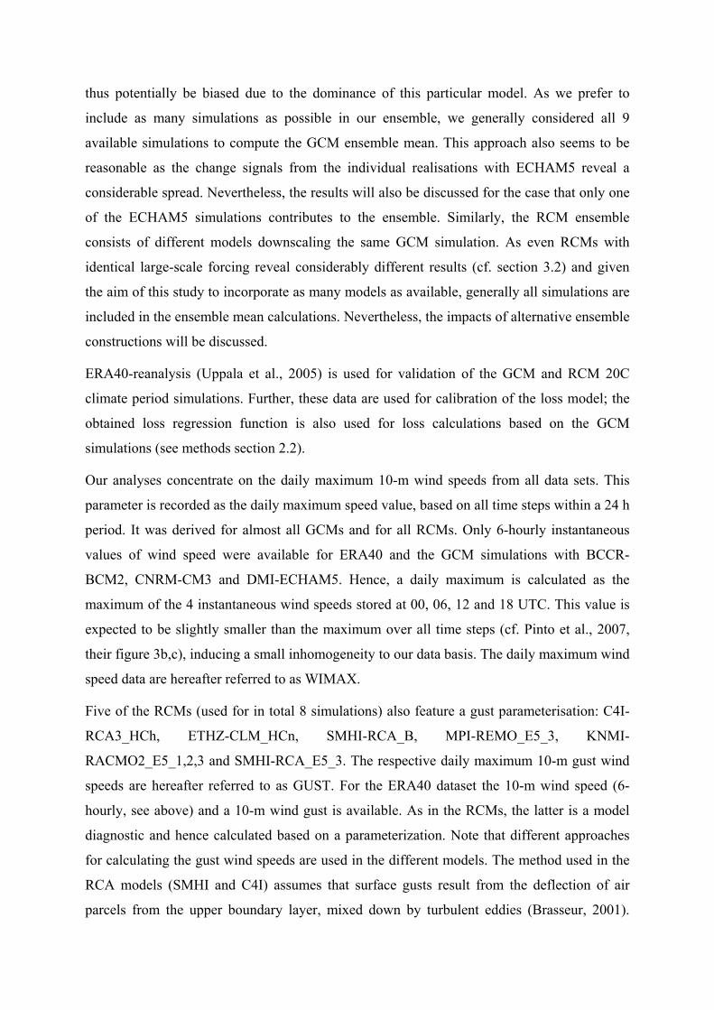
Figure 1. Population density on a 0.25°x0.25° grid is used as a proxy for insured values in the

considered regions for which loss calculations were performed (unit: inhabitants per km²).

Figure 2. Daily maximum wind speed (WIMAX), 98th percentile in the GCM simulations

a) absolute values for 20C (unit: m/s)

Figure 2. Daily maximum wind speed (WIMAX), 98th percentile in the GCM simulations

b) ACC signals A1B-20C: magnitude of changes is displayed by black iso-lines (unit: m/s), coloured areas indicate statistical significance above 0.9 (Student-T-test).

Figure 3. Ensemble Mean of 98th percentile of WIMAX in the GCM simulations

a) absolute values for 20C (unit: m/s)

b) anomaly GCM ensemble (20C) relative to ERA40 (unit: m/s)

c) ACC signal A1B-20C: magnitude of changes is displayed by black iso-lines (unit:

m/s), coloured areas indicate statistical significance above 0.9 (Student-T-test)

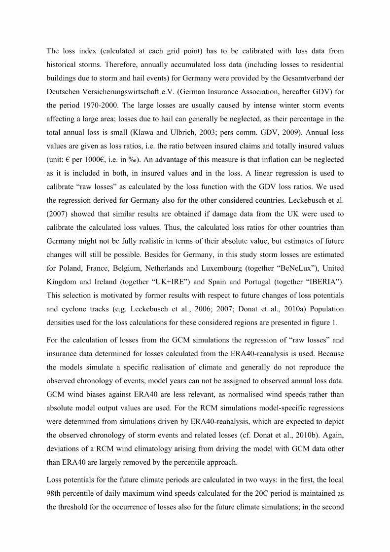
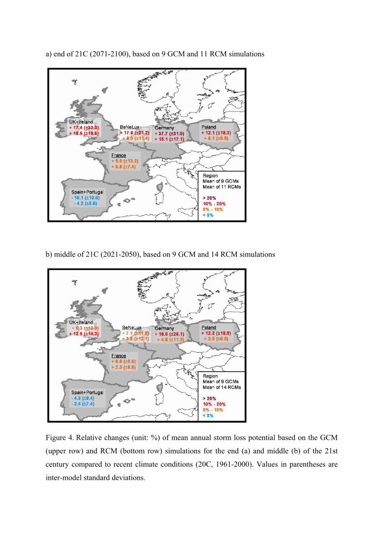
a) end of 21C (2071-2100), based on 9 GCM and 11 RCM simulations

b) middle of 21C (2021-2050), based on 9 GCM and 14 RCM simulations

Figure 4. Relative changes (unit: %) of mean annual storm loss potential based on the GCM

(upper row) and RCM (bottom row) simulations for the end (a) and middle (b) of the 21st

century compared to recent climate conditions (20C, 1961-2000). Values in parentheses are

inter-model standard deviations.

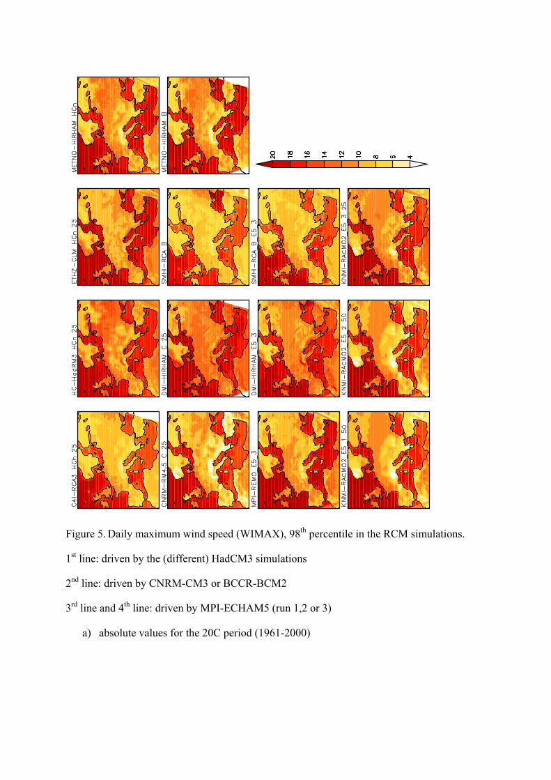
Figure 5. Daily maximum wind speed (WIMAX), 98th percentile in the RCM simulations.

1st line: driven by the (different) HadCM3 simulations

2nd line: driven by CNRM-CM3 or BCCR-BCM2

3rd line and 4th line: driven by MPI-ECHAM5 (run 1,2 or 3)

a) absolute values for the 20C period (1961-2000)

Figure 5. Daily maximum wind speed (WIMAX), 98th percentile in the RCM simulations.

1st line: driven by the (different) HadCM3 simulations, 2nd line: driven by CNRM-CM3 or

BCCR-BCM2, 3rd line and 4th line: driven by MPI-ECHAM5 (run 1,2 or 3)

b) ACC signals for 98th percentile of WIMAX in the RCM simulations, all results are for

the future period 2071-2100, except for METNO_HIRHAM_HCn*, METNO-

HIRHAM_B* and CNRM-RM4.5_C* (only integrated until 2050) signals for the

period 2021-2050 are presented. Magnitude of changes is displayed by black iso-lines

(unit: m/s), coloured areas indicate statistical significance above 0.9 (Student-T-test).

Figure 6. RCM-Ensemble Mean of ACC signal for 98th percentile of WIMAX in the future

scenario simulations. Magnitude of changes is displayed by black iso-lines (unit: m/s),

coloured areas indicate statistical significance above 0.9 (Student-T-test).

a) A1B (2021-2050) – 20C

b) A1B (2071-2100) – 20C

Figure 7. Probability of loss potential changes for the future climate period end of 21C (2071-

2100) compared to 20C (1961-2000) without adaptation of the loss threshold, based on all

possible model combinations of GCMs (green curve), RCMs (blue curve) and all available

GCM and RCM scenario (red curve) simulations. The red shaded areas mark the range where

90% of the change signals (between 5th and 95th percentile) based on all model combinations

are found.

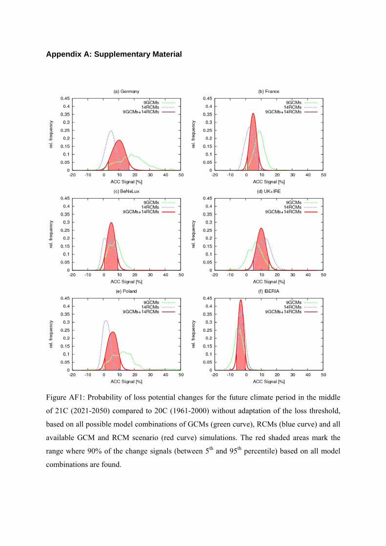
Appendix A: Supplementary Material

Figure AF1: Probability of loss potential changes for the future climate period in the middle

of 21C (2021-2050) compared to 20C (1961-2000) without adaptation of the loss threshold,

based on all possible model combinations of GCMs (green curve), RCMs (blue curve) and all

available GCM and RCM scenario (red curve) simulations. The red shaded areas mark the

range where 90% of the change signals (between 5th and 95th percentile) based on all model

combinations are found.

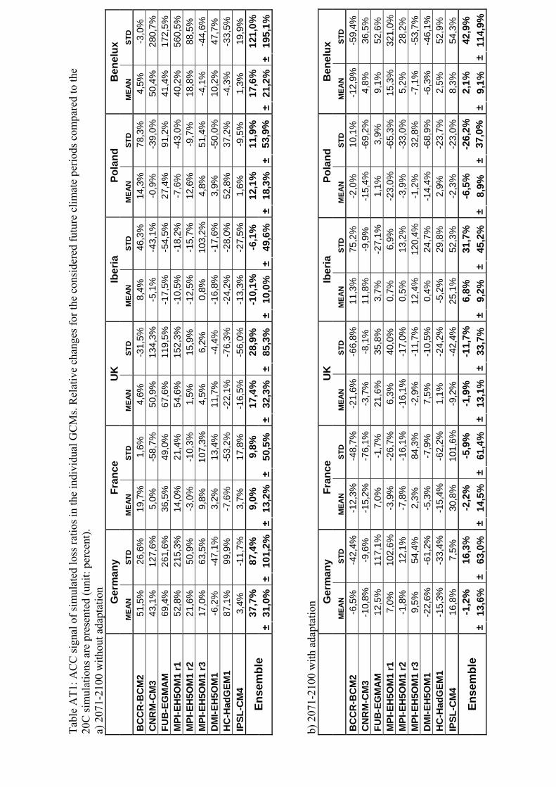
Tabl

e A

T1: A

CC

sign

al o

f sim

ulat

ed lo

ss ra

tios i

n th

e in

divi

dual

GC

Ms.

Rel

ativ

e ch

ange

s for

the

cons

ider

ed fu

ture

clim

ate

perio

ds c

ompa

red

to th

e 20

C si

mul

atio

ns a

re p

rese

nted

(uni

t: pe

rcen

t).

a) 2

071-

2100

with

out a

dapt

atio

n

Ger

man

y Fr

ance

U

K

Iber

ia

Pola

nd

Ben

elux

MEA

N

STD

M

EAN

ST

D

MEA

N

STD

M

EAN

ST

D

MEA

N

STD

M

EAN

ST

D

BC

CR

-BC

M2

51

,5%

26,6

%

19

,7%

1,6%

4,6%

-31,

5%

8,

4%

46

,3%

14,3

%

78

,3%

4,5%

-3,0

%

CN

RM

-CM

3

43,1

%

12

7,6%

5,0%

-58,

7%

50

,9%

134,

3%

-5,1

%

-4

3,1%

-0

,9%

-39,

0%

50,4

%

28

0,7%

FU

B-E

GM

AM

69,4

%

26

1,6%

36,5

%

49

,0%

67,6

%

11

9,5%

-1

7,5%

-5

4,5%

27

,4%

91,2

%

41

,4%

172,

5%

MPI

-EH

5OM

1 r1

52,8

%

21

5,3%

14,0

%

21

,4%

54,6

%

15

2,3%

-1

0,5%

-1

8,2%

-7

,6%

-43,

0%

40,2

%

56

0,5%

M

PI-E

H5O

M1

r2

21

,6%

50,9

%

-3

,0%

-10,

3%

1,

5%

15

,9%

-12,

5%

-15,

7%

12,6

%

-9

,7%

18,8

%

88

,5%

M

PI-E

H5O

M1

r3

17

,0%

63,5

%

9,

8%

10

7,3%

4,

5%

6,

2%

0,

8%

10

3,2%

4,

8%

51

,4%

-4,1

%

-4

4,6%

D

MI-E

H5O

M1

-6

,2%

-47,

1%

3,

2%

13

,4%

11,7

%

-4

,4%

-16,

8%

-17,

6%

3,9%

-50,

0%

10,2

%

47

,7%

H

C-H

adG

EM1

87

,1%

99,9

%

-7

,6%

-53,

2%

-2

2,1%

-7

6,3%

-24,

2%

-28,

0%

52,8

%

37

,2%

-4,3

%

-3

3,5%

IP

SL-C

M4

3,

4%

-1

1,7%

3,7%

17,8

%

-1

6,5%

-5

6,0%

-13,

3%

-27,

5%

1,6%

-9,5

%

1,

3%

19

,9%

37,7

%

87

,4%

9,0%

9,8%

17,4

%

28,9

%

-1

0,1%

-6

,1%

12,1

%

11,9

%

17

,6%

121,

0%

Ense

mbl

e ±

31,0

%

± 10

1,2%

±13

,2%

±50

,5%

±

32,3

%±

85,3

%

±10

,0%

±

49,6

%

±18

,3%

±53

,9%

±

21,2

%

± 19

5,1%

b)

207

1-21

00 w

ith a

dapt

atio

n

G

erm

any

Fran

ce

UK

Ib

eria

Po

land

B

enel

ux

M

EAN

ST

D

MEA

N

STD

M

EAN

ST

D

MEA

N

STD

M

EAN

ST

D

MEA

N

STD

B

CC

R-B

CM

2

-6,5

%

-4

2,4%

-12,

3%

-48,

7%

-2

1,6%

-6

6,8%

11,3

%

75,2

%

-2

,0%

10,1

%

-1

2,9%

-59,

4%

CN

RM

-CM

3

-10,

8%

-9

,6%

-15,

2%

-76,

1%

-3

,7%

-8,1

%

11

,8%

-9

,9%

-15,

4%

-69,

2%

4,

8%

36

,5%

FU

B-E

GM

AM

12,5

%

11

7,1%

7,

0%

-1

,7%

21,6

%

35

,8%

3,7%

-27,

1%

1,

1%

3,

9%

9,

1%

52

,6%

M

PI-E

H5O

M1

r1

7,

0%

10

2,6%

-3

,9%

-26,

7%

6,

3%

40

,0%

0,7%

6,9%

-23,

0%

-65,

3%

15

,3%

321,

0%

MPI

-EH

5OM

1 r2

-1,8

%

12

,1%

-7,8

%

-1

6,1%

-16,

1%

-17,

0%

0,

5%

13

,2%

-3,9

%

-3

3,0%

5,2%

28,2

%

MPI

-EH

5OM

1 r3

9,5%

54,4

%

2,

3%

84

,3%

-2,9

%

-1

1,7%

12,4

%

120,

4%

-1

,2%

32,8

%

-7

,1%

-53,

7%

DM

I-EH

5OM

1

-22,

6%

-6

1,2%

-5,3

%

-7

,9%

7,5%

-10,

5%

0,

4%

24

,7%

-14,

4%

-68,

9%

-6

,3%

-46,

1%

HC

-Had

GEM

1

-15,

3%

-3

3,4%

-15,

4%

-62,

2%

1,

1%

-2

4,2%

-5,2

%

29

,8%

2,9%

-23,

7%

2,

5%

52

,9%

IP

SL-C

M4

16

,8%

7,5%

30,8

%

10

1,6%

-9

,2%

-42,

4%

25

,1%

52

,3%

-2,3

%

-2

3,0%

8,3%

54,3

%

-1

,2%

16,3

%

-2

,2%

-5,9

%

-1

,9%

-11,

7%

6,8%

31,7

%

-6

,5%

-26,

2%

2,1%

42,9

%

Ense

mbl

e ±

13,6

%

± 63

,0%

±

14,5

%±

61,4

%

±13

,1%

±33

,7%

±

9,2%

±

45,2

%

±8,

9%

±37

,0%

±

9,1%

±

114,

9%

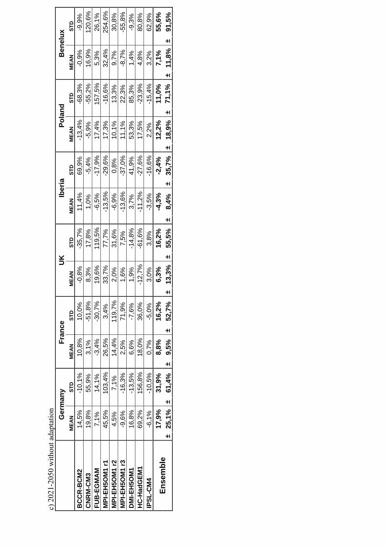
c) 2

021-

2050

with

out a

dapt

atio

n

Ger

man

y Fr

ance

U

K

Iber

ia

Pola

nd

Ben

elux

MEA

N

STD

M

EAN

ST

D

MEA

N

STD

M

EAN

ST

D

MEA

N

STD

M

EAN

ST

D

BC

CR

-BC

M2

14

,5%

-10,

1%

10

,8%

10

,0%

-0,8

%

-3

5,7%

11,4

%

69

,9%

-13,

4%

-68,

3%

-0

,9%

-9,9

%

CN

RM

-CM

3

19,8

%

55

,9%

3,1%

-51,

8%

8,

3%

17

,8%

1,0%

-5,4

%

-5

,9%

-55,

2%

16

,9%

120,

6%

FUB

-EG

MA

M

7,

1%

14

,1%

-3,4

%

-3

0,7%

19,6

%

11

9,5%

-6

,5%

-17,

9%

17,4

%

15

7,5%

5,

3%

26

,1%

M

PI-E

H5O

M1

r1

45

,5%

103,

4%

26,5

%

3,4%

33,7

%

77

,7%

-13,

5%

-29,

6%

17,3

%

-1

6,6%

32,4

%

25

4,6%

M

PI-E

H5O

M1

r2

4,

5%

7,

1%

14

,4%

11

9,7%

2,0%

31,6

%

-6

,9%

0,8%

10,1

%

13

,3%

9,7%

30,8

%

MPI

-EH

5OM

1 r3

-9,6

%

-1

6,3%

2,5%

71,9

%

1,

6%

7,

5%

-1

3,6%

-3

7,0%

11

,1%

22,3

%

-8

,7%

-55,

8%

DM

I-EH

5OM

1

16,8

%

-1

3,5%

6,6%

-7,6

%

1,

9%

-1

4,8%

3,7%

41,9

%

53

,3%

85,3

%

1,

4%

-9

,3%

H

C-H

adG

EM1

69

,2%

156,

8%

18,0

%

36,0

%

-1

2,7%

-6

1,6%

-11,

2%

-27,

6%

17,5

%

-2

3,9%

4,8%

80,8

%

IPSL

-CM

4

-6,1

%

-1

0,5%

0,7%

-5,0

%

3,

0%

3,

8%

-3

,5%

-16,

6%

2,2%

-15,

4%

3,

2%

62

,9%

17,9

%

31

,9%

8,8%

16,2

%

6,

3%

16

,2%

-4,3

%

-2

,4%

12,2

%

11,0

%

7,

1%

55

,6%

En

sem

ble

±25

,1%

±

61,4

%

±9,

5%

±52

,7%

±

13,3

%±

55,5

%

±8,

4%

±35

,7%

±

18,9

%±

71,1

%

±11

,8%

±

91,5

%

Tabl

e A

T2: A

CC

sign

al o

f los

ses c

alcu

late

d in

the

indi

vidu

al R

CM

scen

ario

sim

ulat

ions

. Cha

nge

sign

als A

1B-2

0C w

ithou

t ada

ptat

ion

of th

e lo

ss

thre

shol

d fo

r the

2 fu

ture

per

iods

in th

e m

iddl

e (2

021-

2050

) and

at t

he e

nd o

f 21C

(207

1-21

00).

a) 2

071-

2100

with

out a

dapt

atio

n

Ger

man

y Fr

ance

U

K

Iber

ia

Pola

nd

Ben

elux

MEA

N

STD

M

EAN

ST

D

MEA

N

STD

M

EAN

ST

D

MEA

N

STD

M

EAN

ST

D

C4I

-RC

A3_

HC

h

-2,8

%

3,

6%

-0

,4%

-19,

2%

7,

3%

50

,7%

-6,1

%

-5

9,2%

-8,6

%

-8

3,0%

3,7%

109,

4%

HC

-Had

RM

3_H

Cn

10

,5%

78,1

%

10

,5%

10

9,7%

12,3

%

99

,6%

0,8%

45,4

%

9,

4%

82

,9%

8,2%

281,

4%

ETH

Z-C

LM_H

Cn

19

,0%

65,6

%

9,

3%

16

,7%

27,1

%

20

2,3%

0,6%

32,3

%

8,

0%

10

1,5%

10,8

%

93

,6%

D

MI-H

IRH

AM

_C

2,

5%

-2

2,2%

-2,1

%

-2

1,5%

15,8

%

84

,9%

-7,8

%

-2

5,7%

10,4

%

67,2

%

-1

,7%

-23,

4%

SMH

I-RC

A_B

17,6

%

-6

,2%

15,9

%

99,1

%

23

,0%

57,3

%

7,

9%

12

5,7%

-1

,7%

-24,

0%

4,

4%

10

,6%

M

PI-R

EMO

_E5_

3

5,3%

55,7

%

0,

0%

67

,8%

0,9%

-24,

1%

-3

,5%

-34,

4%

2,

8%

13

,2%

1,8%

81,2

%

DM

I-HIR

HA

M_E

5_3

15

,2%

34,1

%

12

,1%

39

,0%

12,7

%

-3

1,8%

-3,5

%

-1

4,5%

19,6

%

351,

7%

9,

1%

72

,3%

K

NM

I-RA

CM

O2_

E5_1

54,8

%

11

4,0%

8,

7%

6,

2%

63

,6%

288,

0%

-1

1,8%

8,

3%

20

,4%

20

,0%

39,6

%

25

2,2%

K

NM

I-RA

CM

O2_

E5_2

14,3

%

26

,7%

14,8

%

37,8

%

35

,4%

10,2

%

-5

,1%

60,0

%

-3

,7%

-40,

3%

9,

9%

10

,2%

K

NM

I-RA

CM

O2_

E5_3

33,6

%

27

4,6%

-1

,7%

-13,

4%

8,

5%

36

,7%

-7,9

%

-0

,9%

14,1

%

128,

7%

4,

3%

35

,1%

SM

HI-R

CA

_E5_

3

-4,5

%

-9

,9%

-3,9

%

-3

8,4%

-2,6

%

-1

7,3%

-9,8

%

-3

0,5%

-4,3

%

-1

1,2%

-2,6

%

-1

4,2%

15,1

%

55

,8%

5,7%

25,8

%

18

,5%

68

,8%

-4,2

%

9,

7%

6,

1%

55

,2%

8,0%

82,6

%

Ense

mbl

e ±

17,1

%

± 83

,8%

±

7,4%

±

49,9

%

±18

,6%

±99

,1%

±

5,6%

±

53,0

%

±9,

9%

±11

7,6%

±11

,4%

±

101,

2%

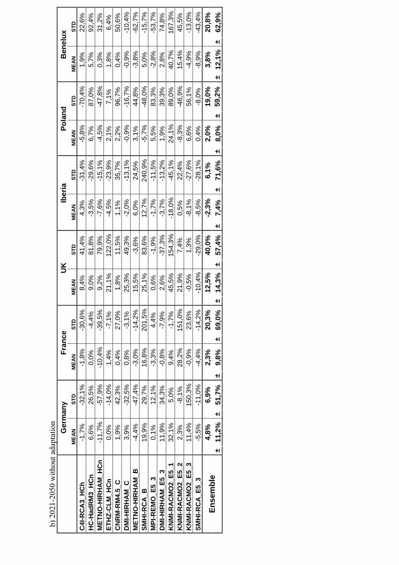
b) 2

021-

2050

with

out a

dapt

atio

n

Ger

man

y Fr

ance

U

K

Iber

ia

Pola

nd

Ben

elux

MEA

N

STD

M

EAN

ST

D

MEA

N

STD

M

EAN

ST

D

MEA

N

STD

M

EAN

ST

D

C4I

-RC

A3_

HC

h

-1,7

%

-3

2,1%

-1,8

%

-3

0,6%

8,4%

41,4

%

4,

3%

-3

1,4%

-5,8

%

-7

0,4%

1,9%

22,6

%

HC

-Had

RM

3_H

Cn

6,

6%

26

,5%

0,0%

-4,4

%

9,

0%

81

,8%

-3,5

%

-2

9,6%

6,7%

87,0

%

5,

7%

92

,4%

M

ETN

O-H

IRH

AM

_HC

n

-11,

7%

-5

7,9%

-10,

4%

-39,

5%

9,

2%

79

,9%

-7,6

%

-1

5,1%

-4,5

%

-4

7,8%

0,3%

31,2

%

ETH

Z-C

LM_H

Cn

0,

0%

-1

4,0%

1,4%

-7,1

%

21

,1%

122,

0%

-4,5

%

-2

3,9%

2,1%

7,1%

1,8%

6,4%

C

NR

M-R

M4.

5_C

1,9%

42,3

%

0,

4%

27

,0%

1,8%

11,5

%

1,

1%

35

,7%

2,2%

96,7

%

0,

4%

50

,6%

D

MI-H

IRH

AM

_C

3,

9%

-3

2,5%

0,8%

-3,1

%

25

,3%

49,3

%

-2

,0%

-13,

1%

-0

,9%

-16,

7%

-0

,9%

-10,

4%

MET

NO

-HIR

HA

M_B

-4,4

%

-4

7,4%

-3,0

%

-1

4,2%

15,5

%

-3

,6%

6,0%

24,5

%

3,

1%

44

,8%

-3,8

%

-6

2,7%

SM

HI-R

CA

_B

19

,9%

29,7

%

16

,8%

201,

5%

25,1

%

83

,6%

12,7

%

24

0,9%

-5

,7%

-48,

0%

5,

0%

-1

5,7%

M

PI-R

EMO

_E5_

3

0,1%

12,1

%

-3

,3%

4,4%

0,6%

-1,9

%

-1

,7%

-11,

5%

5,

5%

83

,3%

-2,8

%

-5

3,7%

D

MI-H

IRH

AM

_E5_

3

11,9

%

34

,3%

-0,8

%

-7

,9%

2,6%

-37,

3%

-3

,7%

-13,

2%

1,

9%

39

,3%

2,8%

74,8

%

KN

MI-R

AC

MO

2_E5

_1

32

,1%

5,0%

9,4%

-1,7

%

45

,5%

154,

3%

-18,

0%

-45,

1%

24

,1%

89,0

%

40

,7%

167,

3%

KN

MI-R

AC

MO

2_E5

_2

2,

3%

-8

,1%

28,2

%

15

1,0%

21

,9%

7,4%

0,5%

22,4

%

-8

,3%

-46,

9%

15

,4%

45,5

%

KN

MI-R

AC

MO

2_E5

_3

11

,4%

150,

3%

-0,9

%

23

,6%

-0,5

%

1,

3%

-8

,1%

-27,

6%

6,

6%

56

,1%

-4,9

%

-1

3,0%

SM

HI-R

CA

_E5_

3

-5,5

%

-1

1,0%

-4,4

%

-1

4,2%

-10,

4%

-29,

0%

-8

,5%

-28,

1%

0,

4%

-8

,0%

-8,9

%

-4

3,4%

4,8%

6,9%

2,3%

20,3

%

12

,5%

40

,0%

-2,3

%

6,

1%

2,

0%

19

,0%

3,8%

20,8

%

Ense

mbl

e ±

11,2

%

± 51

,7%

±

9,8%

±

69,0

%

±14

,3%

±57

,4%

±

7,4%

±

71,6

%

±8,

0%

±59

,2%

±

12,1

%

± 62

,9%

Spatio-temporal impact of climate change on the activityand voltinism of the spruce bark beetle, Ips typographus

A N N A M A R I A J O N S S O N *, G U S T A F A P P E L B E R G *, S U S A N N E H A R D I N G w and L A R S

B A R R I N G *, z*Department of Physical Geography and Ecosystems Analysis, Geobiosphere Science Centre, Lund University, Solvegatan 12, SE-

223 62 Lund, Sweden, wDepartment of Agriculture and Ecology, Faculty of Life Sciences, University of Copenhagen, Thorvaldsensvej

40, DK-1871 Frederiksberg C, Denmark, zRossby Centre, Swedish Meteorological and Hydrological Institute, SE-601 76

Norrkoping, Sweden

Abstract

The spruce bark beetle Ips typographus is one of the major insect pests of mature Norway

spruce forests. In this study, a model describing the temperature-dependent thresholds

for swarming activity and temperature requirement for development from egg to adult

was driven by transient regional climate scenario data for Sweden, covering the period of

1961–2100 for three future climate change scenarios (SRES A2, A1B and B2). During the

20th century, the weather supported the production of one bark beetle generation per

year, except in the north-western mountainous parts of Sweden where the climate

conditions were too harsh. A warmer climate may sustain a viable population also in

the mountainous part; however, the distributional range of I. typographus may be

restricted by the migration speed of Norway spruce. Modelling suggests that an earlier

timing of spring swarming and fulfilled development of the first generation will

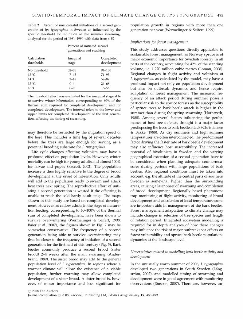
significantly increase the frequency of summer swarming. Model calculations suggest

that the spruce bark beetle will be able to initiate a second generation in South Sweden

during 50% of the years around the mid century. By the end of the century, when

temperatures during the bark beetle activity period are projected to have increased by

2.4–3.8 1C, a second generation will be initiated in South Sweden in 63–81% of the years.

The corresponding figures are 16–33% for Mid Sweden, and 1–6% for North Sweden.

During the next decades, one to two generations per year are predicted in response to

temperature, and the northern distribution limit for the second generation will vary. Our

study addresses questions applicable to sustainable forest management, suggesting that

adequate countermeasures require monitoring of regional differences in timing of

swarming and development of I. typographus, and planning of control operations during

summer periods with large populations of bark beetles.

Keywords: forest damage, impact modelling, Sweden, temperature

Received 31 March 2008; revised version received 12 July 2008 and accepted 18 July 2008

Introduction

A variety of biological effects of the recent climate

warming have been observed as phenological changes

of plant and animal species across Europe (Menzel et al.,

2006). Insects are highly sensitive to changes in climate.

Their metabolic rate is dictated by ambient temperature,

and their activity and development therefore respond

strongly to even minor changes in temperature. Hence,

phenology and developmental rate may change in

response to changes in temperature and, for multivol-

tine insect species, the number of generations per year

may be affected (Ayres & Lombardero, 2000; Volney &

Fleming, 2000). Also, mobility and geographical distri-

bution of insect species may change as a result of global

warming, some species increasing their geographical

range, others moving their limits of distribution

towards north or into higher elevations in mountainous

regions (Williams & Liebhold, 2002; Carroll et al., 2003).

Factors such as fragmentation of vegetation and migra-

tion speed of vegetation may prevent or delay theCorrespondence: Anna Maria Jonsson, tel. 1 46 46 222 94 10,

e-mail: Anna_Maria.Jonsson@nateko.lu.se

Global Change Biology (2009) 15, 486–499, doi: 10.1111/j.1365-2486.2008.01742.x

r 2008 The Authors486 Journal compilation r 2008 Blackwell Publishing Ltd

impact of climate change. The species-specific response

will depend on life-history pattern and interactions

with other species (Harrington & Stork, 1995). These

changes in life cycle and distribution may have pro-

found effects on the dynamics of ecosystems. Distur-

bances are principal driving factors in forest ecosystem

development and dynamics, and phytophagous insects

and pathogens may act as important agents in distur-

bance processes. Further, through their potential impact

on forest health and sustainability of forest manage-

ment, some herbivorous insects call for a specific con-

cern. Models simulating the impact of different climate

variables on insect performance, combined with data

from climate change scenarios, are valuable tools for

assessing how an insect species may be affected by

climate change (Strand, 2000; Bommarco, 2001; Wil-

liams & Liebhold, 2002; Logan et al., 2003).

The Eurasian spruce bark beetle Ips typographus

L. (Coleoptera, Scolytinae) is recognized as one of the

most destructive pests of mature Norway spruce [Picea

abies (L.) Karst.] forests, and periodic large-scale out-

breaks have killed millions of spruce trees in Central

and Northern Europe (Christiansen & Bakke, 1988;

Schelhaas et al., 2003). Damage from bark beetle attacks

has increased markedly during the last 15 years, partly

triggered by storm felling events, partly due to favour-

able climatic conditions (Seidl et al., 2007). When avail-

able breeding substrate is no limiting factor for

population growth, as is the case after huge storm

fellings, the populations of spruce bark beetles may

increase dramatically (Økland & Berryman, 2004). At

high population densities, I. typographus is able to

overcome the defence system of the spruce trees, lead-

ing to an increased risk of colonization of living trees.

Physiological stress following severe drought affects the

defensive system of spruce trees, making them more

susceptible to attack (Christiansen & Bakke, 1988).

Warm and dry summer periods may therefore add

significantly to the magnitude of breeding resources.

Swarming in search of suitable breeding material is

affected by two temperature-dependent factors: the

emergence from overwintering can be estimated by a

thermal sum and mass flight is initiated at daily max-

imum temperature above 20 1C (Annila, 1969; Werme-

linger, 2004). The developmental time from egg to

mature bark beetle is determined by the accumulation

of day degrees and can thus be estimated by a thermal

sum (Annila, 1969; Wermelinger & Seifert, 1998; Nether-

er & Pennerstorfer, 2003). In Central Europe, bivoltin-

ism is the rule except at high elevations (Christiansen &

Bakke, 1988). In Sweden, I. typographus is known to

develop one generation per year and only occasionally a

second generation has been initiated in the southern

parts of the country (Tragardh & Butovitch, 1935;

Butovitch, 1938; Jonsson, 2007), whereas two bark beetle

generations per year are common in Denmark (Harding

& Ravn, 1985).

A process model describing spruce bark beetle activ-

ity and development has been developed and tested

with two regional climate change scenarios covering the

two time-slices 1961–1990 and 2071–2100 for two sites in

the southern, boreo-nemoral part of Sweden (Jonsson

et al., 2007). The results indicated that two generations

per year may occur frequently at both sites by the end of

the 21st century. The results, however, do not tell when

bivoltinism will become frequent and do not indicate

how large the part of the country that will be affected by

the life-cycle changes. The aim of this study is therefore

to provide insights into the spatial and temporal impact

of a gradually changing climate on the swarming and

voltinism of I. typographus. We applied the process

model to new sets of climate model data covering the

transient period of 1961–2100 to simulate temperature-

dependent swarming and development of I. typogra-

phus. The impact of climate change was assessed for the

whole of Sweden, covering three forest vegetation zones

(boreo-nemoral, southern-boreal and boreal conditions).

Bark beetle model simulations were carried out for the

SRES (Special Report on Emission Scenarios) future

scenarios A2, A1B and B2 (Nakicenovic & Swart, 2000).

Material and methods

Modelling bark beetle activity and development

Here, we give the outline for the process model describ-

ing spruce bark beetle activity and development, a

detailed description and discussion of the scientific

background is given in Jonsson et al. (2007). Model

performance has been evaluated with data from Danish

(Jonsson et al., 2007) and Swedish monitoring (Jonsson,

2007). Daily mean temperature (Tmean) and daily max-

imum temperature (Tmax) at 2 m above ground were

used for model calculations. Thermal sums (TDD)

expressed as degree-days (dd) above a threshold (T0)

were calculated as TDD 5S(Tmean�T0), where T0 was set

to 1 5 1C (Annila, 1969). Spring swarming (A), com-

pleted development of first generation (B), summer

swarming (C) and thermal sum from initiation of sec-

ond generation (D) were calculated for each grid cell

(i.e. the spatial resolution of climate model data):

A) Two thermal requirements were specified for in-

itiation of spring swarming (mass flight in spring): (i) a

thermal sum of TDD 5 120 dd for emergence after hiber-

nation and (ii) a daily maximum temperature exceed-

ing 1 20 1C (Tmax41 20 1C) (The threshold of 20 1C

was, however, adjusted to 1 16 1C in the model calcula-

tions due to properties of climate data, see ‘Climate

S PAT I O - T E M P O R A L I M PA C T O F C L I M A T E C H A N G E O N I P S T Y P O G R A P H U S 487

r 2008 The AuthorsJournal compilation r 2008 Blackwell Publishing Ltd, Global Change Biology, 15, 486–499

model data’). Egg development was modelled to start

on the seventh day after swarming, accounting for

preoviposition period (Wermelinger & Seifert, 1999)

and time to produce half of the egg clutch (Anderbrant,

1990).

B) The development time from egg to adult bark

beetle was set to a temperature sum interval with the

lower limit of 625 dd and the upper limit of 750 dd,

accounting for natural variation in microclimate and

light exposure (Harding & Ravn, 1985). The lower limit

represents development in sunexposed trees and the

upper limit development in shaded trees. In nature, a

continuum of breeding conditions will result in an

extended period of time when the new generation of

bark beetles completes development, however, with a

skewed distribution towards the lower limit as the

spruce bark beetle prefers brood trees that are sunex-

posed. The date for completed development of the first

generation was calculated for both the lower and upper

limit of thermal sum.

C) Summer swarming of the first filial generation was

modelled to occur on the first day with Tmax41 20 1C

(adjusted to 16 1C, cf. A), with the additional require-

ment that the daily mean temperature had not yet fallen

below 15 1C during autumn (Annila, 1969). This addi-

tional requirement was set to account for scattered

unseasonally warm days.

D) The development of the second generation was

modelled to start on the seventh day after the onset of

summer swarming (cf. section A). As for the first

generation, two thermal sums (based on lower and

upper limits of thermal sum requirements) were calcu-

lated from two starting dates generated from both

upper and lower limit for completion of development

of the first generation.

Model sensitivity analysis

The swarming threshold value was evaluated in a

sensitivity analysis, calculating the effect of increasing

and decreasing the threshold with one degree, affecting

timing and frequency of both spring and summer

swarming. The impact of thermal sum for emergence

after hibernation on calculated frequency of summer

swarming was tested by increasing and decreasing the

parameter value with 20%. The specific threshold value

Tmean for inhibition of late summer swarming was

evaluated in a sensitivity analysis using no threshold,

13, 14, 15 and 16 1C for the period of 1961–1990, addres-

sing the issue of uncertainties in parameterization dis-

cussed in Jonsson et al. (2007). The threshold was

evaluated for completed development, and for 60% of

the thermal sum required for completed development

corresponding to the imaginal stage able to survive

overwintering (Wermelinger & Seifert, 1998; Baier

et al., 2007). Data from scenario B2 was used in the

sensitivity tests.

Climate model data

Daily climate data from three climate change runs with

the Rossby Centre Regional Climate Model RCA3 (Kjell-

strom et al., 2005) was used. At the lateral boundaries,

RCA3 was forced with output from three different

global climate model (GCM) runs: two runs with the

ECHAM4/OPYC3 (Roeckner et al., 1999) forced by

greenhouse gas concentrations from the SRES (Nakice-

novic & Swart, 2000) A2 and B2 scenarios and one run

with the ECHAM5/MPI-OM (Jungclaus et al., 2006)

forced by the SRES A1B scenario. The A2 and B2

scenarios were commonly used in the IPCC Third

Assessment Report (Cubasch et al., 2001), whereas the

A1B scenario was highlighted in the recent IPCC Fourth

Assessment Report (IPCC, 2007). The magnitude of

greenhouse gas forcing is higher in the A2 scenario

than in the B2 scenario, and the A1B scenario is inter-

mediate, which cause differences in modelled tempera-

ture development. In the present runs, the RCA3 output

data has a spatial resolution (grid cell size) of about

49 km. The data was split into 30-year periods that were

compared with each other. The periods were 1961–1990

(reference period), 1981–2010, 2011–2040, 2041–2070 and

2071–2100. The period of 1981–2010 represents present

day climate and overlaps the reference period by 10

years. The data for the A2 and B2 runs had a simplified

calendar of 360 days per year inherited from the EC-

HAM4/OPY3 global model, whereas the data for the

A1B run had a real calendar with 365 days per year plus

leap years originating from the ECHAM5/MPI-OM

global model. To simplify the bark beetle model com-

putations, the last day of the leap years was removed, as

this day does not affect the results.

The maximum temperature of a RCA3 grid cell is

modelled to represent an average for the whole area

(49� 49 km) and is therefore lower than the maximum

temperature of point measurements. In a study by

Kjellstrom et al. (2005), the model output was evaluated

with weather observations for the spring and summer

season, i.e. March–May and June–August, and the

simulated maximum temperature was found to be

approximately 4 1C lower than corresponding station

observations. The modelled temperature threshold for

mass swarming was therefore adjusted from 20 1C

(Jonsson et al., 2007) to 16 1C.

In this study, Sweden was divided into three regions:

South Sweden characterized by boreo-nemoral condi-

tions (latitude 55–58.71), Mid Sweden (latitude 58.7–

63.51) characterized by southern-boreal conditions and

488 A . M . J O N S S O N et al.

r 2008 The AuthorsJournal compilation r 2008 Blackwell Publishing Ltd, Global Change Biology, 15, 486–499

North Sweden (latitude 63.5–68.31) characterized by

boreal conditions (Ahti et al., 1968). The results were

analysed for each region.

Results

The projected temperature increase during the main

period of bark beetle activity, from the beginning of

April to the end of August (Fig. 1), was high enough in

all the three climate change scenarios to induce sub-

stantial changes in I. typographus development during

this century. The least temperature increase was pro-

jected for scenario A1b and the highest for scenario A2,

scenario B2 being in-between until the last period when

it was close to scenario A1b.

Spring swarming and development of the first generation

The model indicates that spring swarming can occur

earlier in the season (Fig. 2), due to a combination of an

earlier fulfilment of the temperature sum required for

emergence from overwintering sites and an earlier date

for exceeding the temperature threshold for swarming

activity. In most parts of Sweden, present day climate

sustains a completed development of the first genera-

tion almost every year, a warmer climate will, however,

sustain full development to mature adults also in the

mountainous areas of North Sweden (Fig. 3). A com-

parison between Figs 2 and 3 shows that even though

the climate of the reference period has allowed the

temperature requirements for swarming to be fulfilled

in most parts of Sweden, a viable population may be

established in the mountainous north-eastern part in

response to a warmer climate. In the mountains, spring

swarming is unlikely to occur on a regular basis until

summer temperatures support completed development

during most of the years, and this will not be the case

until the period of 2071–2100 with a projected tempera-

ture increase of 2.5–3.2 1C. Because of higher tempera-

tures, the temperature sums required for completion of

development will be obtained during a gradually short-

er period of days according to all three scenarios,

creating an even earlier completed development of the

first generation than induced by an earlier swarming

only (Fig. 3). The effect was thus calculated to be most

pronounced in the period of 2071–2100 (Table 1). The

lower limit for development (625 dd) is in general

fulfilled approximately 2 weeks earlier than the upper

limit (750 dd); however, the difference between sunex-

posed and shaded brood conditions can be up to a

month in the mountainous regions (Fig. 4). The varia-

tion among years, calculated as standard deviation, is

on average 10 days over the country for all scenarios

and 30-year periods, but reaches above 20 days in the

mountainous north-western part.

Summer swarming and development of the secondgeneration

The initiation of a second generation of I. typographus

depends on the fulfilled development of the first gen-

eration, in combination with temperatures sufficiently

high for swarming. Model calculations suggest that the

spruce bark beetle will be able to initiate a second

generation in South Sweden in up to 10% of the years

during the period of 2011–2040 and in 30–49% of the

years during the period of 2041–2070 with a projected

temperature increase of 0.4–1.5 and 1.4–2.2 1C, respec-

tively (Fig. 5). A second generation may also occur in

large parts of Mid Sweden and along the north-eastern

coast according to scenario A2. By the end of the

century, when temperatures during the bark beetle

activity period are projected to have increased by

2.4–3.8 1C according to the different emission scenarios,

a second generation will be initiated in South Sweden in

63–81% of the years. The corresponding figures for Mid

Sweden are 16–33%, and 1–6% for North Sweden (Fig.

5). The time of initiation will, however, not advance in a

continuous way with temperature increase (Fig. 6). This

is due to a more frequent occurrence of swarming at

later dates. The timing and frequency are affected by the

lower and upper limit used for calculating completed

development of the first generation, with an average

difference of 9.5 days within the 30-year periods. The

variation between years of each 30-year period in the

timing of initiation of the second generation was calcu-

lated to increase with temperature during the 21st

century in South Sweden, from a few days to � 8 days.

The timing was calculated to vary within 3–7 days at the

end of the century in North Sweden.

4

3.5

3

2.5

2

1.5

°C

1

0.5

01961–1990 1981–2010 2011–2040 2041–2070 2071–2100

Fig. 1 Changes in average mean temperature from the begin-

ning of April to the end of August. The future periods were

compared with the period of 1961–1990 for the southern (&),

middle (*) and northern (�) part of Sweden. For each period, the

stems show the temperature increase in the different parts of the

country according to scenario A2 (– –), A1b (—) and B2 (- - -).

S PAT I O - T E M P O R A L I M PA C T O F C L I M A T E C H A N G E O N I P S T Y P O G R A P H U S 489

r 2008 The AuthorsJournal compilation r 2008 Blackwell Publishing Ltd, Global Change Biology, 15, 486–499

1961–1990 1981–2010 2011–2040 2041–2070 2071–2100

A2

A1B

B2

August

July

June

May

April

Fig. 2 Modelled timing (mean of 30 years) of spring swarming of Ips typographus according to scenario A2, A1B and B2 for the period of

1961–2100.

October

September

August

July

June

2011–20401961–1990 1981–2010 2041–2070 2071–2100

A2

A1B

B2

Fig. 3 Modelled timing (mean of 30 years) of completed development of the first generation of Ips typographus, using the lower limit of

thermal sum (625 dd) reflecting sunexposed breeding sites, according to scenario A2, A1B and B2 for the period of 1961–2100.

490 A . M . J O N S S O N et al.

r 2008 The AuthorsJournal compilation r 2008 Blackwell Publishing Ltd, Global Change Biology, 15, 486–499

For the rare events in the late 20th century when

temperature was high enough to induce the initiation of

a second generation, the autumn temperature was in

general high enough for obtaining the lower, but not the

upper, temperature sum for completed development.

The larger the temperature increase, the higher the

probability that the accumulated temperature after

completed summer swarming will exceed both the

upper and lower limit for completed development

and thus sustain the production of a fully developed

second generation (Fig. 7). The scenario calculations for

the period of 2041–2071 suggest that the upper tem-

perature sum will be reached in 55–79% of the years in

which a second generation has been initiated in South

Sweden, and the corresponding figures for the end of

the 21st century is 93–98%.

Sensitivity tests

The calculated frequency of summer swarming was not

largely affected by the swarming threshold within the

range of 15–17 1C (Fig. 8), and a 20% increase or

decrease of the thermal sum required for emergence

after hibernation affected the outcome in less than 1% of

the grid cells regardless of geographical region and time

period. The frequency of summer swarming was, how-

ever, highly dependent on the daily mean temperature

threshold for inhibition of summer swarming (Fig. 9).

The threshold sensitivity test, performed with tempera-

ture data for scenario B2 for the period of 1961–1990,

showed that the calculated ratio of brood initiations that

did not reach the adult stage necessary for a successful

overwintering was close to zero using a threshold mean

temperature of 15 1C (Table 2). However, about 50% of

Table 1 Changes in modelled timing of spring swarming and

completed development of the first generation of Ips typogra-

phus in Sweden

Variable (unit)

Part of

Sweden

Scenario

B2

Scenario

A1B

Scenario

A2

Earlier spring

swarming (days)

South 16 17 24

Mid 16 20 20

North 13 15 19

Earlier completed

development (days)

South 26 26 33

Mid 26 30 32

North 20 22 26

The changes were calculated as the difference in average

timing for the period of 2071–2100 and 1961–1991 for three

climate change scenarios A2, A1B and B2.

30

25

20

15

10

5

0

A2

A1B

B2

1961–1990 1981–2010 2011–2040 2041–2070 2071–2100

Fig. 4 Difference in number of days between completed development of the first generation of Ips typographus in breeding material at

sunexposed sites (lower limit of temperature sum, 625 dd) and at shaded sites (upper limit, 750 dd) according to scenario A2, A1B and B2

for the period of 1961–2100.

S PAT I O - T E M P O R A L I M PA C T O F C L I M A T E C H A N G E O N I P S T Y P O G R A P H U S 491

r 2008 The AuthorsJournal compilation r 2008 Blackwell Publishing Ltd, Global Change Biology, 15, 486–499

100

1961–1990

A2

A1B

B2

1981–2010 2011–2040 2041–2070 2071–2100

80

60

40

20

0

Fig. 5 Frequency (% of years) of swarming and initiation of a second generation of Ips typographus, calculated from the lower limit of

thermal sum for completed development of the first generation, according to scenario A2, A1B and B2 for the period of 1961–2100.

1961–1990

A2

A1B

B2

1981–2010 2011–2040 2041–2070 2071–2100

August

July

June

Fig. 6 Modelled timing (mean of 30 years) of summer swarming of Ips typographus based on the lower limit of thermal sum for complete

development, according to scenario A2, A1B and B2 for the period of 1961–2100.

492 A . M . J O N S S O N et al.

r 2008 The AuthorsJournal compilation r 2008 Blackwell Publishing Ltd, Global Change Biology, 15, 486–499

the clutches initiated at late swarming events, corre-

sponding to the upper limit of completed development

of the first generation, would not have been able to

complete maturation feeding. In comparison, a thresh-

old of 16 1C had only marginal effect on further redu-

cing the calculated risk for unsuccessful brood

initiations, whereas the risk increased substantially

using thresholds of 13 and 14 1C. With no threshold,

up to 86% of initiated second generations were calcu-

lated as unsuccessful.

Discussion

Spatio-temporal changes in spruce bark beetle activity andvoltinism

The projected temperature increase varies among sea-

sons, being somewhat higher in winter than in summer

(Kjellstrom et al., 2005). The climate model data used in

this study indicated a temperature increase for Sweden

between 2.4 and 3.8 1C during the main period of bark

beetle activity, corresponding to an increase in annual

Lower limit

Upper limit

A2

A1B

B2

A2

A1B

B2

1961–1990 1981–2010 2011–2040 2041–2070 2071–2100

100

80

60

40

20

0

Fig. 7 Frequency (% of years) of completed development of a second generation of Ips typographus, calculated with a timing of initiation

of the second generation given the lower and upper thermal sum limits for completion of development of the first generation, according

to scenario A2, A1B and B2 for the period of 1961–2100.

S PAT I O - T E M P O R A L I M PA C T O F C L I M A T E C H A N G E O N I P S T Y P O G R A P H U S 493

r 2008 The AuthorsJournal compilation r 2008 Blackwell Publishing Ltd, Global Change Biology, 15, 486–499

mean temperature of 3.4–4.4 1C at the end of this

century. This modelling study showed that warmer

climate could drastically change activity, voltinism

and geographical range of I. typographus. Assessments

with all three scenarios indicated that the temperature

requirements for spring swarming will be fulfilled ear-

lier than at present day climate, the effect being most

pronounced in the mid and south part of Sweden. This,

in combination with raised temperatures during brood

development, will allow an increased frequency of

initiation of a second generation in summer in South

Sweden and, according to the temperature projections

of the warmer scenario A2, also in large parts of

Mid Sweden and along the eastern coast. All three

climate change scenarios indicated a higher frequency

of brood initiation than of completed development of

the second generation in South Sweden for the first half

of the 21st century, when the projected temperature

increase is less than 2.5 1C. In a warmer climate, the

discrepancy will gradually decrease. During the next

decades, inter-annual variations in weather conditions

will create opportunities for one or two generations

per year and the northern limit for a second generation

will vary between years in response to temperature

conditions.

I. typographus is present in North Sweden; however,

the current climate does not support a viable population

in the mountainous north-western part. Furthermore,

Norway spruce is currently not present at higher alti-

tudes in this area (Ahti et al., 1968). Although warmer

climate will allow colonization of I. typographus into this

region, the spread and population establishment will be

determined by the presence of the host tree, and the

expansion of the distributional range of I. typographus

1961–1990 1981–2010 2011–2040 2041–2070 2071–2100

10

8

6

4

2

0

–1°C

+1°C

Fig. 8 Sensitivity test of the temperature threshold for swarming, affecting the timing of both spring and summer swarming. The maps

in the upper row show the increase in modelled frequency (% of years) of a second generation when the threshold of 16 1C was reduced

by one degree, and the maps in the lower row show the decrease in modelled frequency when the swarming threshold was increased by

one degree. Calculations were based on the lower limit of completed development of the first generation, according to data from scenario

B2 for the period of 1961–2100.

No threshold 13°C

B2

14°C 15°C 16°C100

80

60

40

20

0

Fig. 9 Influence of temperature threshold for inhibition of summer swarming (13–16 1C) on modelled frequency (% of years) of

swarming and initiation of a second generation. Calculations were based on the lower limit of completed development of the first

generation according to data for the period of 1961–1990.

494 A . M . J O N S S O N et al.

r 2008 The AuthorsJournal compilation r 2008 Blackwell Publishing Ltd, Global Change Biology, 15, 486–499

may therefore be restricted by the migration speed of

the host. This includes a time lag of several decades

before the trees are large enough for serving as a

potential breeding substrate for I. typographus.

Life cycle changes affecting voltinism may have a

profound effect on population levels. However, winter

mortality can be high for young adults and almost 100%

for larvae and pupae (Faccoli, 2002). The population

increase is thus highly sensitive to the degree of brood

development at the onset of hibernation. Only adults

will add to the population ready to swarm and attack

host trees next spring. The reproductive effort of initi-

ating a second generation is wasted if the offspring is

unable to reach the cold hardy adult stage. The maps

shown in this study are based on completed develop-

ment. However, as callow adults in the stage of matura-

tion feeding, corresponding to 60–100% of the thermal

sum of completed development, have been shown to

survive overwintering (Wermelinger & Seifert, 1998;

Baier et al., 2007), the figures shown in Fig. 7 may be

somewhat conservative. The frequency of a second

generation being able to survive overwintering may

thus be closer to the frequency of initiation of a second

generation for the first half of this century (Fig. 5). Bark

beetles commonly produce a second brood (sister

brood) 2–4 weeks after the main swarming (Ander-

brant, 1989). The sister brood may add to the general

population level of I. typographus. In regions where a

warmer climate will allow the existence of a viable

population, further warming may allow completed

development of a sister brood. A sister brood is, how-

ever, of minor importance and less significant for

population growth in regions with more than one

generation per year (Wermelinger & Seifert, 1999).

Implications for forest management

This study addresses questions directly applicable to

sustainable forest management, as Norway spruce is of

major economic importance for Swedish forestry in all

parts of the country, accounting for 42% of the standing

volume, i.e. 1.270 million cubic metres (Loman, 2008).

Regional changes in flight activity and voltinism of

I. typographus, as calculated by the model, may have a

profound impact not only on population development

but also on outbreak dynamics and hence require

adaptation of forest management. The increased fre-

quency of an attack period during summer poses a

particular risk to the spruce forests as the susceptibility

of spruce trees to bark beetle attack is higher in the

summer than during the spring swarming (Horntvedt,

1988). Among several factors influencing the perfor-

mance of host tree defence, drought is a major factor

predisposing the trees to bark beetle attack (Christiansen

& Bakke, 1988). As dry summers and high summer

temperatures are often interconnected, the predominant

factor driving the faster rate of bark beetle development

may also influence host susceptibility. The increased

potential of bivoltinism in Sweden and the varying

geographical extension of a second generation have to

be considered when planning adequate countermea-

sures during periods with large populations of bark

beetles. Also regional conditions must be taken into

account; e.g. the altitude of the central parts of southern

Sweden is somewhat higher than the surrounding

areas, causing a later onset of swarming and completion

of brood development. Regionally based pheromone

trap monitoring of flight activity, monitoring of brood

development and calculation of local temperature sums

are important aids in management of the bark beetles.

Forest management adaptation to climate change may

include changes in selection of tree species and length

of rotation period. Integrated ecosystem modelling is

required for in depth analyses of how these changes

may influence the risk of major outbreaks via effects on

forest vulnerability and spruce bark beetle populations

dynamics at the landscape level.

Uncertainties related to modelling bark beetle activity anddevelopment

In the unusually warm summer of 2006, I. typographus

developed two generations in South Sweden (Lang-

strom, 2007), and modelled timing of swarming and

development were in good agreement with monitoring

observations (Jonsson, 2007). There are, however, un-

Table 2 Percent of unsuccessful initiations of a second gen-

eration of Ips typographus in Sweden as influenced by the

specific threshold for inhibition of late summer swarming,

analysed for the period of 1961–1990 with data from s B2

Calculation

thresholds

Percent of initiated second

generations not reaching

Imaginal

stage

Completed

development

No threshold 52–86 94–100

13 1C 7–45 71–95

14 1C 2–18 52–87

15 1C 0–4 24–68

16 1C 0–0 6–56

The threshold effect was evaluated for the imaginal stage able

to survive winter hibernation, corresponding to 60% of the

thermal sum required for completed development, and for

completed development. The interval refers to the lower and

upper limits for completed development of the first genera-

tion, affecting the timing of swarming.

S PAT I O - T E M P O R A L I M PA C T O F C L I M A T E C H A N G E O N I P S T Y P O G R A P H U S 495

r 2008 The AuthorsJournal compilation r 2008 Blackwell Publishing Ltd, Global Change Biology, 15, 486–499

certainties related to model parameterization, as

detailed experimental knowledge rarely covers the en-

tire range of environmental conditions and variations in

response, accounting for population-specific adapta-

tions to local climate conditions. In addition, experi-

mentally determined temperature thresholds have a

spatial and temporal context, such as a constant labora-

tory temperature or meteorological point data from a

station near the monitoring site, that may not perfectly

match the spatial and temporal context of climate

model output representing grid cell averages

(49 km� 49 km). In this study, the swarming threshold

had to be adjusted to match modelled grid cell daily

maximum temperature while at the same time account-

ing for existing model biases, as it was not possible to

make a complete and, from a climatological point of

view, correct adjustment of modelled temperature data.

The climate model biases vary somewhat between

months and regions (Kjellstrom et al., 2005); however,

the calculated frequency of a second generation was not

sensitive to swarming threshold parameterization with-

in the tested range of 15–171.

Different developmental thresholds (T0) have been

found and used in various studies. Annila (1969) ob-

served development at 5 1C for 38%, 42% and 9% of the

egg, larvae and pupae, respectively. Wermelinger &

Seifert (1998) determined the stage specific thresholds,

using curve-fitting methods to produce two sets of

extrapolated temperature threshold values. For model-

ling purposes, we used the threshold of 5 1C in combi-

nation with daily mean temperature, as this has been

used in several Scandinavian field studies, and data

from these studies were used in model parameteriza-

tion and evaluation (Jonsson et al., 2007). In addition,

the daily average temperature after spring swarming is

commonly above the highest suggested temperature

threshold; however, the use of higher temperature

thresholds would have increased the sensitivity to

biases in climate model data. For instance, with a daily

mean temperature of 12 1C and a model bias of 1 1 1C,

the error is 14% using a threshold of 5 1C, but with a

threshold of 8 1C, the error increases to 25%.

Temperatures above 30 1C are less optimal for devel-

opment of I. typographus (Wermelinger & Seifert, 1998,

1999) and prolonged exposure to temperatures above

45 1C can be lethal (Annila, 1969). Daily mean tempera-

ture, used in calculations of development, was not

projected in any scenario to reach above 30 1C. How-

ever, bark temperature can be much higher than air

temperature and differ largely even within a brood tree

dependent on sun exposure (Annila, 1969). It is influ-

enced by momentary changes in cloudiness and wind

in combination with bark-specific properties such as

albedo, insulation capacity and water content. Model-

ling of microclimatological conditions was outside the

scope of this study; however, microclimatological con-

ditions were taken into account using a temperature

sum interval for calculating completed development.

Today, the southern part of Sweden is ‘one bark beetle

generation ahead’ of northern Sweden, in the sense that

a large discrepancy exists between calculated frequen-

cies of fully developed first generation and initiation of

the second generation. The magnitude of this discre-

pancy is determined by the modelled inhibition of

summer swarming. The threshold of 15 1C is in agree-

ment with common knowledge of I. typographus being

univoltine in Sweden (Eidmann & Klingstrom, 1990),

and the balance between the risk of unsuccessful initia-

tions and chance of a completed second generation that

may have affected natural selection is optimal in com-

parison with the other temperature thresholds. How-

ever, in multivoltine populations of I. typographus in

Central Europe, the reproductive activity has been

shown to be restricted by short-day photoperiods

(Schopf, 1989; Dolezal & Sehnal, 2007). Therefore, mini-

mum temperatures in combination with a photoperio-

dic threshold are more likely to control the initiation of

a second generation of I. typographus than temperature

alone (Jonsson et al., 2007). In a laboratory study, Dole-

zal & Sehnal (2007) demonstrated that the onset of

diapause in I. typographus was influenced by day length

in combination with temperature conditions, where

high temperatures could offset the effect of short days

and low temperatures could enhance the onset of

diapause. Spruce bark beetles from Central Europe as

well as from Scandinavia were sensitive to the day

length conditions occurring in their natural habitats in

July and beginning of August. Field studies in Austria

found that only spruce bark beetles that had completed

total development at photoperiods before mid August

(� 14.5 h daylight) emerged from brood systems (Baier

et al., 2007). When using a temperature threshold of

15 1C in this study, the modelled northern limit of

summer swarming for the period of 1961–2100 coin-

cided with the end of July–beginning of August in all

climate scenarios. This indicates that the model out-

come is compatible with light influence. Nevertheless,

for more accurate climate change impact assessments

and modelling of weather impact on potential bark

beetle development, improved knowledge of factors

controlling inhibition of summer swarming is required.

A correct estimate is important for evaluation of popu-

lation growth potential.

Uncertainties related to climate model data

The results of this study are dependent on the repre-

sentativity and quality of the regional climate model

496 A . M . J O N S S O N et al.

r 2008 The AuthorsJournal compilation r 2008 Blackwell Publishing Ltd, Global Change Biology, 15, 486–499

data. However, modelled climate deviates from

observed climate due to properties of gridded data,

natural variability, model biases and uncertainties from

a range of sources. For example, for the period of 1961–

2040, the projected timing of swarming and fulfilled

development of the first generation is a few days later in

scenario A1B than in scenario A2 and B2 for the South

and Mid of Sweden, resulting in a lower calculated

frequency of summer swarming. Because the emission

scenarios do not differ much before the middle of this

century, the temperature difference between scenario

runs is mainly caused by natural variability injected by

different initial conditions in combination with differ-

ences between the two model generations ECHAM4

and ECHAM5. Comparing the multi-model ensemble

of the GCMs, van Ulden & van Oldenborgh (2006)

found that ECHAM5 shows skill in representing the

basic pressure patterns and large-scale atmospheric

flow over the north Atlantic–European region com-

pared with weather observations, i.e. ERA-40 dataset

(Uppala et al., 2005).

We have analysed in total three different regional

climate scenarios, downscaled by one regional climate

model from output of two versions (i.e. development

generations) of a coupled global modelling system.

There are, however, uncertainties associated with the

choice of climate model data. Scenario simulations

carried out by a multitude of climate models indicate

a best estimate in temperature increase in global mean

temperature of 2.4, 2.8 and 3.4 1C at the end of the

21st century, with a likely range of 1.4–3.8, 1.7–4.4

and 2.0–5.4 1C for scenario B2, A1B and A2, respectively

(IPCC, 2007). The forcing GCM has, in general, larger

influence on climate model uncertainty than the regio-

nal climate model or the choice of emission scenario

(Deque et al., 2007). Other combinations of regional and

GCMs would thus indicate different strength in the

regional climate change signal (Christensen & Christen-

sen, 2007), thus influencing model estimates of timing

and frequency of swarming and development of

I. typographus. The bark beetle model has been run by

climate data for scenario A2 and B2, from another

combination of regional and global climate models

(HadRM3H) (Jonsson et al., 2007) also showing a high

frequency of bivoltinism for the period of 2071–2100. It

is, however, not possible to compare any spatial and

temporal patterns as only two grid cells were analysed.

In a modelling study for Norway, using another impact

model and different sets of climate data, Lange et al.

(2006) showed that bivoltinism can move northwards

by 600 km by the end of the century according to

scenario B2. This corresponds to our findings of a

second generation being present in the central part of

Mid Sweden.

Conclusions

The modelling, with a projected temperature increase

by the end of this century of 2.4–3.8 1C during the bark

beetle activity period, suggested significant spatio-

temporal changes in the life cycle and voltinism of

I. typographus in a gradually changing climate. The

frequency of summer swarming and of completed

development of a second generation can increase due

to earlier spring swarming and faster development of

the first generation. The northern limit for a second

generation will vary between years in response to

temperature conditions. Model calculations indicated

that I. typographus will shift from univoltine to primarily

bivoltine in South Sweden and a viable population may

be established in the north-western mountainous parts.

The expansion of the distributional range of I. typogra-

phus may, however, be restricted by the migration speed

of Norway spruce. Changes in the timing of phenolo-

gical events will gradually affect the recommendations

for timely bark beetle management operations. For

adequate timing of countermeasures during periods

with large populations of bark beetles, regional mon-

itoring of swarming, development and probability of

bivoltinism will be required.

Acknowledgements

This work was carried out within the EU/FP6 ENSEMBLESproject (GOCE-CT-2003-505539). Anonymous reviewers arethanked for valuable comments to an earlier version of themanuscript.

References

Ahti T, Hamet-Ahti L, Jalas J (1968) Vegetation zones and their

sections in northwestern Europe. Annales Botanici Fennici, 5,

169–211.

Anderbrant O (1989) Reemergence and second brood in the bark

beetle Ips typographus. Holarctic Ecology, 12, 494–500.

Anderbrant O (1990) Gallery construction and oviposition of the

bark beetle Ips typographus (Coleoptera: Scolytidae) at different

breeding densities. Ecological Entomology, 15, 1–8.

Annila E (1969) Influence of temperature upon the development

and voltinism of Ips typographus L. (Coleoptera, Scolytidae).

Annales Zoologici Fennici, 6, 161–208.

Ayres MP, Lombardero MJ (2000) Assessing the consequences of

global change for forest disturbance from herbivores and

pathogens. The Science of the Total Environment, 262, 263–286.

Baier P, Pennerstorfer J, Schopf A (2007) PHENIPS – a compre-

hensive phenology model of Ips typographus (L.) (Col., Scoly-

tinae) as a tool for hazard rating of bark beetle infestation.

Forest Ecology and Management, 249, 171–186.

Bommarco R (2001) Using matrix models to explore the influence

of temperature on population growth of arthropod pests.

Agricultural and Forest Entomology, 3, 275–283.

S PAT I O - T E M P O R A L I M PA C T O F C L I M A T E C H A N G E O N I P S T Y P O G R A P H U S 497

r 2008 The AuthorsJournal compilation r 2008 Blackwell Publishing Ltd, Global Change Biology, 15, 486–499

Butovitch V (1938) Om granbarkborrens massforokning i sodra

Dalarna. Norrlands Skogvardsforbunds Tidskrift, 1938, 91–126.

Carroll A, Taylor SW, Regniere J, Safranyik L (2003) Effects of

climate change on range expansion by the mountain pine

beetle in British Columbia. In: Mountain Pine Beetle Symposium:

Challenges and Solutions (eds Shore TL, Brooks JE, Stone JE),

October 30–31, 2003, Kelowna, BC. Natural Resources Canada,

Canadian Forest Service, Pacific Forestry Centre, Information

Report BC-X-399, Victoria, BC, pp. 223–232.

Christensen JH, Christensen OB (2007) A summary of the

PRUDENCE model projections of changes in European cli-

mate by the end of this century. Climate Change, 81, 7–30.

Christiansen E, Bakke A (1988) The spruce bark beetle of Eurasia.

In: Dynamics of Forest Insect Populations (ed. Berryman AA), pp.

479–503. Plenum Publishing Corporation, New York and

London.

Cubasch U, Meehl GA, Boer GJ et al. (2001) Projections of future

climate change. In: Climate Change 2001: The Scientific Basis.

Contribution of Working Group I to the Third Assessment Report of

the Intergovernmental Panel on Climate Change (eds Houghton JT,

Ding Y, Griggs DJ, Noguer M, van der Linden PJ, Dai X,

Maskell K, Johnson CA), pp. 525–582. Cambridge University

Press, Cambridge, UK and New York, NY, USA.

Deque M, Rowell DP, Luthi D et al. (2007) An intercomparison of

regional climate simulations for Europe: assessing uncertain-

ties in model projection. Climate Change, 81, 53–70.

Dolezal P, Sehnal F (2007) Effects of photoperiod and tempera-

ture on the development and diapause of the bark beetle Ips

typographus. Journal of Applied Entomology, 131, 165–173.

Eidmann HH, Klingstrom A (1990) Skadegorare i skogen. LTs

forlag, Stockholm, pp. 303–307 (in Swedish).

Faccoli M (2002) Winter mortality in sub-corticolous popu-

lations of Ips typographus (Coleoptera, Scolytidae) and its para-

sitoids in the south-eastern Alps. Journal of Pest Science, 75,

62–68.

Harding S, Ravn HP (1985) Seasonal activity of Ips typographus L.

(Col., Scolytidae) in Denmark. Zeitschrift fur Angewandte

Entomologie, 99, 123–131.

Harrington R, Stork NE (eds) (1995) Insects in a Changing Envir-

onment. Academic Press, London.

Horntvedt R (1988) Resistance of Picea abies to Ips typographus:

tree response to monthly inoculations with Ophiostoma poloni-

cum, a beetle transmitted blue stain fungus. Scandinavian

Journal of Forest Research, 3, 107–114.

IPCC (2007) Climate change 2007: the physical science basis.

Contribution of working group I to the fourth assessment.

Report of the Intergovernmental Panel on Climate Change (eds

Solomon S, Qin D, Manning M, Chen Z, Marquis M, Averyt

KB, Tignor M, Miller HL), pp. 996. Cambridge University

Press, Cambridge, UK and New York, NY, USA.

Jonsson AM (2007) Berakning av den attatandade granbarkbor-

rens temperaturberoende svarmning och utveckling ar 2006.

In: Overvakning av Insektsangrepp – Slutrapport fran Skogsstyr-

elsens Regeringsuppdrag (ed. Svensson L), pp. 98–100 Skogsstyr-

elsen Meddelanden 1:2007. Skogsstyrelsen, Jonkoping,

Sweden.

Jonsson AM, Harding S, Barring L, Ravn HP (2007) Impact of the

climate change on the population dynamics of Ips typographus

in southern Sweden. Agricultural and Forest Meteorology, 146,

70–81.

Jungclaus JH, Keenlyside N, Botzet M et al. (2006) Ocean circula-

tion and tropical variability in the coupled model ECHAM5/

MPI-OM. Journal of Climate, 19, 3952–3972.

Kjellstrom E, Barring L, Gollvik S et al. (2005) A 140-year simula-

tion of European climate with the new version of the Rossby Centre

regional atmospheric climate model (RCA3). Reports on Meteor-

ology and Climatology, No. 108, December 2005, Swedish

Meteorological and Hydrological Institute, Norrkoping, Swe-

den, 54 pp.

Lange H, Økland B, Krokene P (2006) Thresholds in the life cycle

of the spruce bark beetle under climate change. Interjournal for

Complex Systems, 1648, 1–10.

Langstrom B (2007) Bilaga 5 Svarmningskontroll av barkborrar

pa Asa och Tonnersjohedens forsoksparker. In: Overvakning av

Insektsangrepp – Slutrapport fran Skogsstyrelsens Regeringsupp-

drag (ed. Svensson L), pp. 44–57, Skogsstyrelsen Meddelanden

1:2007. Skogsstyrelsen, Jonkoping, Sweden.

Logan JA, Regniere J, Powell JA (2003) Assessing the impact of

global warming on forest pest dynamics. Frontiers in Ecology

and Environment, 1, 130–137.

Loman JO (ed.) (2008) Statistical Yearbook of Forestry 2008. Official

Statistics of Sweden, Swedish Forest Agency, J o nk o ping.

Menzel A, Sparks TH, Estrella N et al. (2006) European pheno-

logical response to climate change matches the warming

pattern. Global Change Biology, 12, 1969–1976.

Nakicenovic N, Swart R (eds) (2000) Emission Scenarios, a

Special Report of Working Group III of the Intergovernmental Panel

on Climate Change. Cambridge University Press, Cambridge, UK.

Netherer S, Pennerstorfer J (2003) Parameters relevant for mod-

eling the potential development of Ips typographus (Coleoptera:

Scolytidae). Integrated Pest Management Reviews, 6, 177–184.

Økland B, Berryman A (2004) Ressource dynamics plays a key

role in regional fluctuations of the spruce bark beetles Ips

typographus. Agricultural and Forest Entomology, 6, 141–146.

Roeckner E, Bengtsson L, Feichter J, Lelieveld J, Rodhe H (1999)

Transient climate change simulations with a coupled atmo-

sphere-ocean GCM including the tropospheric sulfur cycle.

Journal of Climate, 12, 3004–3032.

Schelhaas MJ, Nabuurs GJ, Schuck A (2003) Natural distur-

bances in the European forests in the 19th and 20th centuries.

Global Change Biology, 9, 1620–1633.

Schopf A (1989) The effect of photoperiod on the induction of the

imaginal diapause of Ips typographus (L.) (Col., Scolytidae).

Journal of Applied Entomology, 107, 275–288.

Seidl R, Baier P, Rammer W, Schopf A, Lexer M (2007) Modelling

tree mortality by bark beetle infestation in Norway spruce

forests. Ecological Modelling, 206, 383–399.

Strand JF (2000) Some agrometeorological aspects of pest and

disease management for the 21st century. Agricultural and

Forest Meteorology, 103, 73–82.

Tragardh I, Butovitch V (1935) Redogorelse for barkborrekam-

panjen efter stormharjningarna 1931–1932. Meddelanden fran

Statens Skogsforsoksanstalt, 28, 1–268.

Uppala SM, Kallberg PW, Simmons AJ et al. (2005) The ERA-40

re-analysis. Quarterly Journal of the Royal Meteorological Society,

131, 2961–3012.

498 A . M . J O N S S O N et al.

r 2008 The AuthorsJournal compilation r 2008 Blackwell Publishing Ltd, Global Change Biology, 15, 486–499

van Ulden AP, van Oldenborgh GJ (2006) Large-scale atmo-

spheric circulation biases and changes in global climate model

simulations and their importance for climate change in

Central Europe. Atmospheric Chemistry and Physics, 6,

863–881.

Volney WJA, Fleming RA (2000) Climate change and impacts of

boreal forest insects. Agriculture, Ecosystems and Environment,

82, 283–294.

Wermelinger B (2004) Ecology and management of the spruce

bark beetle Ips typographus – a review of recent research. Forest

Ecology and Management, 202, 67–82.

Wermelinger B, Seifert M (1998) Analysis of the temperature

dependent development of the spruce bark beetle Ips typogra-

phus (L.) (Col., Scolytidae). Journal of Applied Entomology, 122,

185–191.

Wermelinger B, Seifert M (1999) Temperature-dependent repro-

duction of the spruce bark beetle Ips typographus, and analysis

of the potential population growth. Ecological Entomology, 24,

103–110.

Williams DW, Liebhold AM (2002) Climate change and the

outbreak ranges of two North American bark beetles. Agricul-

tural and Forest Entomology, 4, 87–99.

S PAT I O - T E M P O R A L I M PA C T O F C L I M A T E C H A N G E O N I P S T Y P O G R A P H U S 499

r 2008 The AuthorsJournal compilation r 2008 Blackwell Publishing Ltd, Global Change Biology, 15, 486–499

Ih

Aa

b

a

ARRAA

KNPLBPFHCC

1

tib7miwpc

S

0d

Ecological Modelling 221 (2010) 303–313

Contents lists available at ScienceDirect

Ecological Modelling

journa l homepage: www.e lsev ier .com/ locate /eco lmodel

mpacts of changing frost regimes on Swedish forests: Incorporating coldardiness in a regional ecosystem model

. Rammig a,∗, A.M. Jönsson a, T. Hickler a, B. Smith a, L. Bärring a,b, M.T. Sykes a

Geobiosphere Science Centre, Department of Physical Geography and Ecosystems Analysis, Lund University, Sölvegatan 12, SE-22362 Lund, SwedenSMHI Rossby Centre, Swedish Meteorological and Hydrological Institute, SE-60176 Norrköping, Sweden

r t i c l e i n f o

rticle history:eceived 27 October 2008eceived in revised form 5 May 2009ccepted 9 May 2009vailable online 21 June 2009

eywords:orway spruceicea abies (L. Karst.)PJ-GUESSoreal forest productionhysiological tolerancerost hardinessardening/dehardening cycleslimate changelimate extremes

a b s t r a c t

Understanding the effects of climate change on boreal forests which hold about 7% of the global terres-trial biomass carbon is a major issue. An important mechanism in boreal tree species is acclimatization toseasonal variations in temperature (cold hardiness) to withstand low temperatures during winter. Tem-perature drops below the hardiness level may cause frost damage. Increased climate variability underglobal and regional warming might lead to more severe frost damage events, with consequences fortree individuals, populations and ecosystems. We assessed the potential future impacts of changing frostregimes on Norway spruce (Picea abies L. Karst.) in Sweden. A cold hardiness and frost damage modelwere incorporated within a dynamic ecosystem model, LPJ-GUESS. The frost tolerance of Norway sprucewas calculated based on daily mean temperature fluctuations, corresponding to time and temperaturedependent chemical reactions and cellular adjustments. The severity of frost damage was calculated asa growth-reducing factor when the minimum temperature was below the frost tolerance. The hardinessmodel was linked to the ecosystem model by reducing needle biomass and thereby growth according tothe calculated severity of frost damage. A sensitivity analysis of the hardiness model revealed that theseverity of frost events was significantly altered by variations in the hardening rate and dehardening rateduring current climate conditions. The modelled occurrence and intensity of frost events was related to

observed crown defoliation, indicating that 6–12% of the needle loss could be attributed to frost dam-age. When driving the combined ecosystem-hardiness model with future climate from a regional climatemodel (RCM), the results suggest a decreasing number and strength of extreme frost events particularly innorthern Sweden and strongly increasing productivity for Norway spruce by the end of the 21st centuryas a result of longer growing seasons and increasing atmospheric CO2 concentrations. However, accord-ing to the model, frost damage might decrease the potential productivity by as much as 25% early in thecentury.

. Introduction

Boreal forests cover up to 14.7 Mio km2, which is about 11% ofhe earth’s land surface (Bonan and Shugart, 1989). They play anmportant role in global climate by storing about 42 Gt of Car-on in biomass and 200 Gt C in soil organic matter representing.5–10% of the global terrestrial amounts (Jarvis et al., 2001). Cli-ate change will affect these ecosystems not only through changes

n mean conditions – such as impacts of changing temperature,ater availability and atmospheric CO2 concentrations on plantroduction – but also via changes in the frequency and level oflimatic extremes (IPCC, 2007), such as changes in frost regimes,

∗ Corresponding author at: Potsdam Institute for Climate Impact Research, Earthystem Analysis, P.O. Box 60 12 03, 14412 Potsdam, Germany. Tel.: +49 331 288 2454.

E-mail address: Anja.Rammig@pik-potsdam.de (A. Rammig).

304-3800/$ – see front matter © 2009 Elsevier B.V. All rights reserved.oi:10.1016/j.ecolmodel.2009.05.014

© 2009 Elsevier B.V. All rights reserved.

prolonged water stress or drought, or damaging windstorms. Stud-ies with global models point to the likelihood of increased climaticvariability under future greenhouse forcing (IPCC, 2007). A hypoth-esis is that this could lead to an increased frequency of weatherevents beyond plant physiological tolerance thresholds, potentiallyresulting in stress, damage, mortality and changed biogeochemicalcycling in ecosystems.

Cannell and Smith (1986) presented the seemingly paradoxicalhypothesis that climatic warming in the boreal and temperate zoneswill cause increased frost damage due to dehardening or growthonset of trees during mild spells in winter and early spring, leadingto frost damage in subsequent cold periods. Increased frost dam-

age could reduce the positive effect of an extended growing periodand elevated atmospheric CO2 concentrations on forest growth(Woldendorp et al., 2008). In Norway spruce (Picea abies L. Karst.),frost is harmful when the ambient temperature falls below the“hardiness level” (Jönsson, 2005).

3 l Mod

acmLtp2tda

(eRtaBbeKecdSepe(tapb

hm(hcp1foefgcflnprpdne

thaelimurb

04 A. Rammig et al. / Ecologica

Hardiness is the ability of plant cells to tolerate cellular freezingnd occurs during the annual cycle of trees during acclimation toold temperatures. It is controlled by an additive effect of environ-ental factors, such as photoperiod and temperature (Chen and

i, 1978). During the active growth phase, the trees do not havehe potential for hardening. After growth cessation, the hardeningrocess is initiated (Kellomäki et al., 1995; Bigras and Colombo,000) and the trees use their energy resources to develop a freezeolerance (cf. Fuchigami et al., 1982; Harrison et al., 1978). Theehardening process starts with increasing temperatures (Bigrasnd Colombo, 2000).

Seedlings and newly developed shoots are particularly sensitiveCannell and Sheppard, 1982; Sakai and Larcher, 1987), but frostpisodes may also damage needles, bark and roots in mature trees.eversible damage of needles causes ion leakage due to disrup-ion of membrane transport functions and the recovery costs waternd energy (e.g. Sutinen et al., 2001; Linder and Flower-Ellis, 1992;urr et al., 2001). Damaged trees are prone to subsequent attacksy fungal pathogens, which may cause heavy crown defoliation orven kill the tree (Alden and Hermann, 1971; Schoeneweiss, 1975;arlman, 1986; Kowalski, 1991, 1996; Sieber et al., 1995). Jönssont al. (2004) showed that an earlier start of the vegetation periodaused by a warmer climate can increase the risk for spring frostamage on mature Norway spruce (P. abies L. Karst.) in southernweden. This hypothesis is also supported by electrolyte leakagexperiments (Repo et al., 1996) and model simulations for Scotsine (Pinus sylvestris L.) and other tree species in Finland (Kellomäkit al., 1995; Leinonen, 1996; Hänninen et al., 2001). However, Ögren2001) concluded from carbohydrate measurements after freezingreatments that the seasonal hardening and dehardening cyclesnd cold hardiness levels of Norway spruce, Scots pine and lodge-ole pine (Pinus contorta ssp. latifolia Loud.) would be unaffectedy global warming.

Most modelling studies of climate effects on tree frost hardinessave been very detailed in their description of the physiologicalechanisms of the investigated tree species over the annual cycle

e.g. Kellomäki et al., 1995; Leinonen, 1996). However, the modelsave to date only been applied at the site scale under simplifiedlimate change projections, such as a linear increase in mean tem-erature (Cannell and Smith, 1986; Kellomäki et al., 1995; Leinonen,996). Impacts of climate and atmospheric changes on ecosystemunctioning at regional scales may be investigated with the helpf process-based ecosystem models (e.g. Bergh et al., 2003; Kocat al., 2006; Morales et al., 2007). Current models include detailedormulations of physiological processes linking plant gas exchange,rowth, phenology, and neighbourhood interactions to gradualhanges in climate. Mechanisms of response to daily temperatureuctuations, including variations in frost hardiness, are, however,ot included in many current models, or are represented in sim-listic ways that are insufficient to capture the detailed ecosystemesponse. Many studies also use monthly mean values of climatearameters as input to the ecosystem model, so that thresholds foramage or reduced functioning, such as lethal temperatures, mayever be crossed (e.g. Hickler et al., 2004; Morales et al., 2007; Kocat al., 2006).

Thanks to developments in climate modelling, it is now possibleo obtain driving climate data for ecosystem model studies with aigh spatial resolution and realistic characterisation of diurnal vari-tion and extremes of temperature. Regional climate models (RCMs,.g. Christensen et al., 2007; Jacob et al., 2007) describe processeseading to seasonally and regionally non-uniform warming trends

n a more realistic manner compared to coarser-resolution global

odels (general circulation models, GCMs). For example, RCM sim-lations over northern Europe suggest that regional warming mayeduce the seasonal snow cover resulting in a positive albedo feed-ack that enhances the wintertime warming trend (Kjellström,

elling 221 (2010) 303–313

2004). The more limited spatial averaging that occurs in RCMs com-pared to GCMs may result in a better description of possible changesin extremes, such as low temperatures, under greenhouse forcingscenarios (Kjellström et al., 2005, 2007).

In this study, we aimed to address two hypotheses: (1) regionalclimate change will alter the risk for frost damage in mature Nor-way spruce, as a major dominant species of boreal forest in Sweden.(2) The productivity of spruce-dominated forests will be influencedby changes in the risk for frost damage under future climate con-ditions. In order to investigate these hypotheses, we incorporateda detailed physiological model of frost hardiness (Jönsson et al.,2004) and frost damage (Kellomäki et al., 1995; Leinonen, 1996) thataccounts for autumn, mid-winter and spring frost events within anexisting process-based ecosystem model, LPJ-GUESS (Smith et al.,2001). This is a step towards the development of tools for assess-ing the effects of changing frost regimes on forest productivity atthe regional scale. In this paper, we focus on model developmentand evaluation. The outcomes of our study provide first estimatesof changes in the risk of frost damage. We present model generatedhypotheses on the potential impacts of frost damage on the pro-ductivity of Norway spruce in different regions of Sweden underfuture climate conditions, based on RCM-generated high-resolutiontransient daily climate data.

2. Methods

An existing model to calculate the daily frost hardiness (Jönssonet al., 2004) and frost damage (Kellomäki et al., 1995; Leinonen,1996) accounting for autumn, mid-winter and spring frost eventsin Norway spruce was tested and incorporated within the process-based ecosystem model LPJ-GUESS (Smith et al., 2001; Koca et al.,2006). Model performance was evaluated by comparing simulationresults to observed data on needle loss and stand productivity.

2.1. Model descriptions

2.1.1. Ecosystem model (LPJ-GUESS)The generalized ecosystem model LPJ-GUESS (Smith et al., 2001)

combines the mechanistic representations of plant physiologicaland biogeochemical processes of the Lund-Potsdam-Jena DynamicGlobal Vegetation Model (LPJ-DGVM; Sitch et al., 2003) with adetailed description of vegetation structure and dynamics, simi-lar to forest gap models such as FORSKA2 (Prentice et al., 1993). Fortree individuals, the model simulates photosynthesis, respirationand allocation of annually accrued carbon (net primary production,NPP) to leaves, fine roots, sapwood, heartwood and reproductiveorgans, accounting for seasonal changes in needle phenology andadjustments in stomatal conductance. Neighbouring individualscompete for uptake of light and soil water. Population dynamics(establishment and mortality) are influenced by current resourcestatus, demography and the life history characteristics of each sim-ulated species or plant functional type (PFT). In this study, themodel was set up only to simulate growth and dynamics of even-aged stands of Norway spruce (parameters settings see Table 1, allother parameters were inherited from Smith et al. (2001), Sitchet al. (2003), Hickler et al. (2004) and Koca et al. (2006)). Inputdata to the model are daily or monthly mean values of climateparameters (temperature (◦C), precipitation (mm) and incomingshortwave radiation (Wm−2)), atmospheric CO2 concentrations anda soil texture class that governs soil hydrology and heat conduc-

tance. LPJ-GUESS has been applied to simulate north European orboreal vegetation in several previous studies (Badeck et al., 2001;Smith et al., 2001, 2008; Hickler et al., 2004; Koca et al., 2006;Morales et al., 2005, 2007; Zaehle et al., 2006) and has been evalu-ated, for example, using data on growth (Zaehle et al., 2006; Smith

A. Rammig et al. / Ecological Modelling 221 (2010) 303–313 305

Table 1Plant functional type and species parameter settings for simulations of Norwayspruce stands with LPJ-GUESS, all other parameters were inherited from Smith et al.(2001), Hickler et al. (2004) and Koca et al. (2006).

Parameter Unit Value Source

Tree specific parametersCarbon density of sapwood

and heartwood in treeskgC m−3 250 Jaakkola et al. (2006)

Fraction of roots in upper(0–50 cm) and lower(50–150 cm) soil layer

Dimensionless 0.9/0.1 Köstler et al. (1968)

Needleleaf specific parametersLeaf area to sapwood

cross-sectional area ratiom2 m−2 3500 Köstner et al. (2002)

Leaf longevity Years 4 Niinemets andLukjanova (2003)

Fine root turnover Year−1 0.7 Vogt et al. (1996), Li etal. (2003)

Shadetolerant specific parametersSapwood conversion rate Year−1 0.05 Bartelink (2000)

Norway spruce specific parametersExpected longevity under Years 500 Bugmann (1994)

ea

2

fbd“id

Table 2Parameters for the frost hardiness and frost damage model.

Parameters forstandard runs

Description Value and unit

Parameters for hardiness modelHmin Minimum hardiness levela −2 ◦CHmax Maximum hardiness levelc −30 ◦CSaut Start of autumn (start of

hardening)aJulian day 210

Sspr Start of spring (start ofdehardening) for SouthernSwedena

Julian day 1

H∗t Target hardiness levela F (daily mean temperature)

r∗h

Rate of hardeninga 0–1 ◦C/dayr∗

dhRate of dehardeninga 0–5 ◦C/day

Wd Winter dormancya From days 260 to 365

Parameters for calculation of the growth reducing factorb Slope parameterb 0.2 ◦C−1

LT50 “Lethal temperature”c 20 ◦C

where max(value 1, value 2) is a function that selects the maxi-

F(h

lifetime non-stressedconditions

t al., 2008) and carbon fluxes (Morales et al., 2005; Wramneby etl., 2008) for European forests.

.1.2. Hardiness modelCalculations of the hardiness level of Norway spruce were per-

ormed using an updated version of the hardiness model developedy Jönsson et al. (2004). In the hardiness model (Fig. 1B), the har-

◦

iness level Hday ( C) is adjusted on a daily basis, converging to atarget” hardiness level Ht (Fig. 1C, Table 2) according to a harden-ng or dehardening rate (rh or rdh; Fig. 1D and E, Table 2) based onaily mean temperature Tmean (◦C; Fig. 1B). Hday during the summer

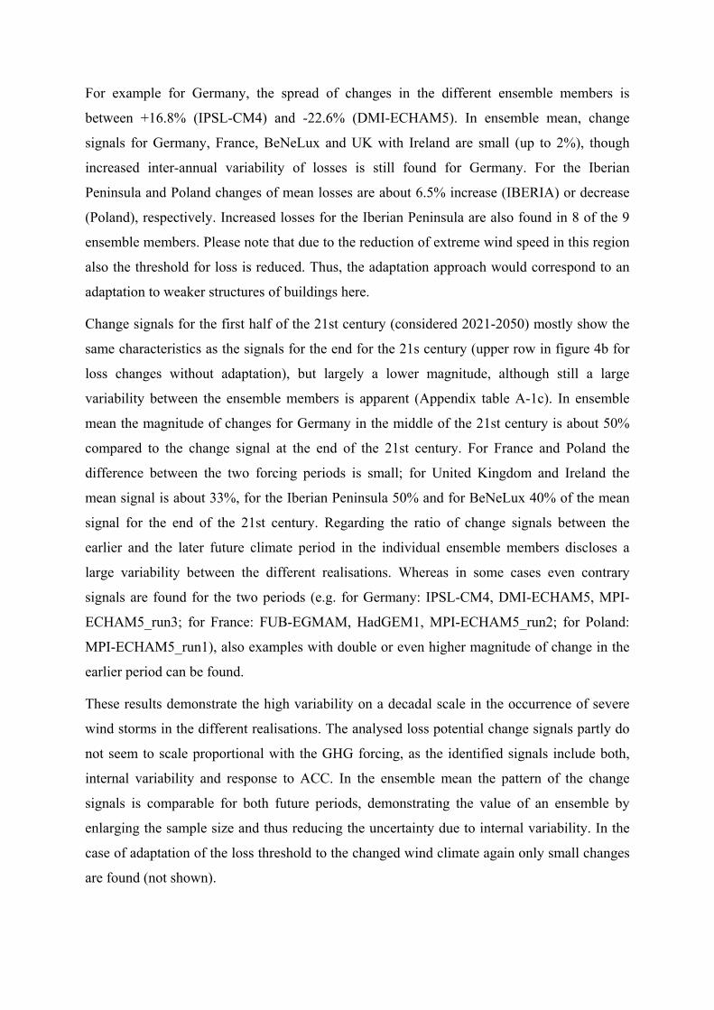
ig. 1. (A) Distribution of the study sites (black dots) over Sweden showing forestry adm55.6–57.9◦N), “Central” (58.0–61.8◦N) and “North” (62.2–67.8◦N) regions. (B) Example ofardiness level. (C–E) Target hardiness (in ◦C), hardening and dehardening rates (in ◦C day

a Values from Jönsson et al. (2004).b Values from Kellomäki et al. (1995).c Values from Bigras and Colombo (2000).

is calculated as

Hday(day + 1) = Hmin

{if Hday(day) + rdh < Hmin

if aggd5 ≥ 120◦C and if day ≤ Saut

(1)

where day is the day of year, Hmin is the minimum hardiness, Saut isthe day of start of autumn (Table 2) and aggd5 are the accumulatedgrowing degree days (◦C), calculated as

aggd5 = aggd5 + max(0, Tmean − 5 ◦C) (2)

mum from two values. Bud burst in Central Sweden occurs after120 degree-days above 5 ◦C (Hannerz, 1994). At the first day of theyear, aggd5 is set to 0 ◦C. During springtime (if day < Saut and if Eq.(1) is not true), then both, hardening and dehardening is possible

inistrative regions; for some analyses the study sites were grouped into “South”a 1-year mean and minimum temperature curve for one site and the corresponding−1) in relation to the ambient mean temperature.

3 l Mod

a

H

H

H

it

H

l

D

wdaDb

F

a

S

wt

2

rTat

g

wtttadaipowrwttakritL

g

b

06 A. Rammig et al. / Ecologica

nd the hardiness Hday is calculated as

day(day + 1) = Hmin if Hday(day) + rdh > Hmin (3)

day(day + 1) = Hday(day) − rh if Hday(day) ≥ Ht (4)

day(day + 1) = Hday(day) + rdh if Hday(day) ≤ Ht (5)

During winter (Wd, Table 2), only hardening is possible and Hdays calculated according to Eq. (4). The hardiness can not fall belowhe maximum hardiness (Hmax, Table 2) and thus

day(day + 1) = Hmax if Hday(day + 1) > Hmax (6)

The daily difference Dday (◦C) between the calculated hardinessevel Hday and the minimum temperature Tmin (◦C).

day = Hday − Tmin,day (7)

as taken to be the main factor determining the degree of frostamage to the trees (Fig. 1B). At a day with Dday > 0, the trees weressumed to experience a frost event. We counted the days whereday > 0 and defined this as the frequency of frost events FFE (num-er of days):

FEyear =365∑d=1

{1 if Dday > 00 if Dday ≤ 0

(8)

Additionally, the size of the frost event SFEday (◦C) was defineds

FEday = max(0, Dday) (9)

hich is the actual amount of the difference Dday if the minimumemperature falls below the hardiness level (Fig. 1B).

.1.3. Frost damage modelBased on the hardiness level and current temperature, a “growth

educing factor” (gfday) was calculated in LPJ-GUESS for each day.he growth reducing factor gives the relative effect of freeze dam-ge for each difference between the hardiness level and minimumemperature Dday (Eq. (1)) according to a logistic function:

fday = 11 + exp(b(Dday − LT50))

(10)

here b is the slope parameter, and Dday is the difference betweenhe hardiness level of the tree and the minimum temperature athe specified day. Thus, Dday was taken as a proxy for the length ofhe cold episode and thus determines the degree of the frost dam-ge. The parameter LT50 (◦C) is defined as the “lethal temperatureifference between the hardiness level and the minimum temper-ture” at which 50% of the trees are damaged, and determines thenflection-point of the curve, depending on the Dday. For the pur-oses of this study, we set LT50 to 20 ◦C, i.e. with Dday = 20 ◦C, 50%f the needles would be killed (Table 2). The slope parameter bas assumed to be 0.2 for the standard simulations. The growth

educing factor is dimensionless and ranges between 0.0 and 1.0,here values <0.1 signify strong damage and values >0.9 signify lit-

le damage (modified after Kellomäki et al., 1995). It was assumedhat frost damage primarily affects trees by causing needle necrosisnd a reduction in carbon assimilation in proportion to the needlesilled (Bigras and Colombo, 2000). The frost damage model thenelates needle loss to the growth reducing factor by using the min-mum daily value obtained for gfday during a simulation year, gfmin,o determine the annual amount of frost damage (modified after

einonen, 1996):

fmin = min(365d=1gfd) (11)

It was thus assumed that the maximum temperature differenceetween the daily minimum temperature and the daily hardiness

elling 221 (2010) 303–313

level on any particular day is an adequate predictor for the frostdamage for that year (Leinonen, 1996). Frost damage was imple-mented at the end of each simulation year based on the gfmin-value:the leaf carbon mass, sapwood mass and accrued NPP of eachaverage individual tree (representing average properties of the sim-ulated trees within a patch) were multiplied by gfmin. Killed needleswere transferred to the litter pool, and killed sapwood to heart-wood. It was assumed that roots were not affected by frost damage.

2.2. Data for model evaluation

Data on crown defoliation from 1999 to 2005 from 122 man-aged Norway spruce stands were obtained from the Swedish ForestAgency. These data were collected in accordance with ICP forestmonitoring (Eichhorn et al., 2006). The site locations range in lat-itude from 51.7 to 67.5◦N, spanning most forest areas in Sweden(Fig. 1A). In these data, crown defoliation is defined as the annualneedle loss, in 5% intervals, relative to a tree of the same type(species, age, size) with full foliage (Eichhorn et al., 2006), andranged between 0 and 35% for the observed forests. The observa-tions on crown defoliation were carried out annually by comparingthe selected tree to a “reference tree”, which is defined as “the besttree with full foliage that could grow at a particular site. . . [with]0% defoliation” (Eichhorn et al., 2006). The density of the observedstands was on average 740 trees ha−1 and average stand age 59years. Observed data of forest stand productivity in Sweden (mea-sured as mean annual stem volume increment, m3 ha−1 yr−1) wereobtained from the Swedish Forest Agency (2007) for the period2001–2005 for the 19 forestry administrative regions of Sweden.

2.3. Environmental driver data

Global atmospheric CO2 concentrations derived from ice-coremeasurements and atmospheric observations (Sitch et al., 2003)were used to drive the model for the historical period of the sim-ulations (see Section 4 below). For the period from 1999 to 2100,projections of CO2 concentrations were used (Joos et al., 2001).

Climate data for the ecosystem model runs were derived fromthree sources: (1) MESAN/ERA40, which is high-resolution (11 km)gridded meteorological data obtained from the mesoscale mete-orological analysis system MESAN (Häggmark et al., 2000) set upto use ERA-40 reanalysis data (Uppala et al., 2005) in combinationwith quality-controlled daily observations from weather stations(Jansson et al., 2007); (2) RCA3/ERA40 are output data from theSMHI Rossby Centre regional climate model RCA3 run for the cli-mate of Europe over the historical period 1961–2004 forced byERA-40 reanalysis data (Uppala et al., 2005) at the lateral bound-aries; and (3) RCA3/ECHAM4/A2 are output data from RCA3 froma simulation covering the period 1961–2100 (Kjellström et al.,2005) with lateral boundary conditions taken from an experimentwith the ECHAM4/OPYC3 general circulation model (Roeckner etal., 1999) forced by the SRES A2 emission scenario. The SRES A2assumes a “regional-economic” development of the future world(Nakicenovic et al., 2000). For both (2 and 3), RCA3 was configuredto have a spatial resolution of 0.5◦ (ca. 50 km) and it was operated ona time step of 30 min. The basic characteristics of RCA3 were eval-uated by Kjellström et al. (2005) and the new land surface schemeis presented by Samuelsson et al. (2006). For all three data sources,the data used were average daily values of temperature (◦C), precip-itation (mm) and total downward shortwave radiation at the landsurface (Wm−2) as well as daily minimum temperature (◦C), all on

a 0.5 × 0.5◦ regular grid covering Sweden.

Because the frost hardiness model is critically sensitive to theinput data for minimum daily temperature (Eq. (7)), it was impor-tant to correct for any bias in the mean and minimum temperaturedata. Three sources of bias were considered: bias that could arise

l Modelling 221 (2010) 303–313 307

fealdqambto‘Rptm(

2

pofaftaasf

2

icmwrutcp

2

upctRi

2

2

upv(eiHHi

Table 3Parameter variations in the hardiness and frost damage model for the sensitivityanalysis.

Simulation Parameter settings

Sensitivity analysis for the hardiness modelH1 StandardH2 Hardening rate +20%H3 Hardening rate −20%H4 Dehardening rate +20%H5 Dehardening rate −20%H6 “Target” hardiness level −50 ◦CH7 Start of autumn day 220 (∼August 8),

daylight ca. 15.2 (S)–16.5(N) hH8 Start of autumn day 230 (∼August 18),

daylight ca. 14.5 (S)–15.5(N) hH9 Start of autumn ca. day 237 (∼August 25;

S)–244 (∼September 1; N), daylight 14 h

Sensitivity analysis for the frost damage modelFNO No frost damageF1 Frost damage model, b = 0.2, LT50 = 20F2 Frost damage model, b = 0.1, LT50 = 20

A. Rammig et al. / Ecologica

rom RCA3, from ECHAM4/OPYC3, and from the up-scaling of mod-lled and observed data to the 0.5 × 0.5◦ grid. Dataset (1) wasssumed to be free from bias. Thus as a ‘Control Period I’, the over-apping period between the MESAN/ERA40 and the RCA3/ERA40atasets from 1998 to 2004 has been used. For this period we canuantify the bias in RCA3 versus observed climate conditions. Welso need to correct for the GCM bias, which is a combination ofodel bias (model imperfections) and natural variability induced

y the initial conditions and the fact that a climate scenario simula-ion is not constrained by observed weather conditions during thebserved reference period. For this purpose we use the overlapping

Control Period II’ from 1961 to 2004 between the RCA3/ERA40 andCA3/ECHAM4/A2 data has been used. To correct the mean tem-erature, a standardization method has been used. The minimumemperature has been corrected using the difference between the

ean and the minimum temperature, and an arithmetic methodSupplementary data).

.4. Modelling protocol

For our study, we applied the model to simulate even-aged,lanted Norway spruce stands at the 122 sites in Sweden for whichbserved frost damage data were available (Fig. 1). Climate dataor the grid cell encapsulating the observed site were used. Standge, density (trees ha−1) and disturbance history were prescribedor the simulation runs in order to get a realistic representation ofhe forest for the study period. For example, a stand with a recordedge of 75 years in 2005 was initialized (planted with spruce treest the density of the observed stand) in the simulation year corre-ponding to calendar year 1930. Tree regeneration was switched offor the remainder of the simulation.

.4.1. Model evaluation runsSimulations under current climate conditions were performed

n order to evaluate the performance of the model. The bias-orrected RCA3/ECHAM4/A2 climate data were used to drive theodel for the period 1930–1990. The simulations then continuedith input from the 8 years of MESAN-ERA40 data, which were

epeated twice. The first 8 years (1990–1998) were used as a “spinp” period in order to achieve an approximate steady state betweenhe simulated forest stand and the climate, the second 8 yearsorresponded to the actual period from 1998 to 2005 (evaluationeriod).

.4.2. Future scenario runsTo explore changes in frost damage and stand productivity

nder future climate conditions at each stand, simulations wereerformed with input from the bias-corrected RCA3/ECHAM4/A2limate data for the entire period 1961–2100. Climate data beforehis period were constructed by repeating the first 10 years of theCA3/ECHAM4/A2 climate dataset the number of times required to

nitialise each stand in the year it was actually planted.

.5. Analysis of model behaviour and performance

.5.1. Sensitivity of the simulated frost hardiness and frost damageTo test the sensitivity of the hardiness model, a range of sim-

lation experiments with different model configurations wereerformed for 1999–2005: simulation H1 corresponds to theersion with standard settings (Table 2). In simulations H2–H9Table 3), only one parameter at a time (OAT-experiments, Saltelli

t al., 2000) was varied. Hardening and dehardening rate was var-ed by +/−20% around the standard value (H2–H5). In simulation6, the maximum hardiness was set to −50 ◦C. In simulations7–H9, the start of autumn was retarded by 10–14 days. Accord-

ngly, changes in the main output variables of the hardiness model,

F3 Frost damage model, b = 0.3, LT50 = 20F4 Frost damage model, b = 0.2, LT50 = 10F5 Frost damage model, b = 0.2, LT50 = 30

namely derivates of FFE (frequency of frost events per year, whenminimum temperature drops below the hardiness level, Eq. (8)) andSFE (size of frost event, Eq. (9)) were analyzed over the simulationperiod (start = 1999, end = 2005, nyears = 6):

- The frequency of frost events over the simulation period.

SumFFE =end∑

y=start

FFEy (12)

- The average of the size of a maximum frost event.

AvSFEmax =∑end

y=startSFEmax,y

nyears(13)

where SFEmax is the largest value of SFE for any day in year y.The results of SumFFE and AvSFEmax were evaluated for the rangeof simulation experiments by ANOVA and pairwise comparisons(unpaired t-test; R statistical software).

The sensitivity of the frost damage model was also evaluatedby a range of simulation experiments, varying the parameters thatdetermine the growth reducing factor (gfday, Eq. (10)), and therebythe needle carbon mass, sapwood mass and accrued NPP of eachaverage individual tree: simulation F1 corresponds to the standardversion with b = 0.2 (Table 3, Kellomäki et al., 1995) and LT50 = 20 ◦C(Bigras and Colombo, 2000). The slope parameter b of the frost dam-age model (Eq. (10)) was varied between 0.1 and 0.3 (simulationsF2 and F3, Table 3). The parameter LT50, which denotes the pointwhere 50% of the needles are damaged, was varied between 10 and30 ◦C (simulation F4 and F5). To quantify the effect of the parametervariations, the “simulated crown defoliation” was used. To calculatesimulated crown defoliation we used the average simulated valuefor needle carbon biomass (kgC m−2) for the period 1999–2005. Theneedle carbon biomass of simulation FNO (no frost damage, Table 3)was set to 100%. Simulated crown defoliation was calculated forsimulations F1–F5 as the average needle carbon mass expressed asa percentage of the value from the FNO simulation.

2.5.2. Evaluation of the ecosystem model performanceIn order to evaluate the skill of the ecosystem model, we com-

pared simulated stem wood volume increments (m3 ha−1 yr−1)with average values for Swedish forestry administrative regions

308 A. Rammig et al. / Ecological Modelling 221 (2010) 303–313

F ., 200s reque( s the um uartil

baifww2at(1

uctoaiowddnsntdmduo

2c

o(a

ig. 2. Results of the sensitivity analysis of the frost hardiness model (Jönsson et alites. The simulation runs H1–H9 are described in Table 3. Given are the sum of the fAvSFEmax , Eq. (13)). The black line within the box denotes the median, the box give

inimum and maximum of the distribution within the range of 1.5 times the interq

y grouping the 122 sites into 21 forestry administrative regionsnd computing an average value for each region. Stem volumencrement was estimated from carbon mass increment obtainedrom LPJ-GUESS simulations. For conversion of carbon mass to stem

ood volume, it was assumed that 65% of the total carbon massould contribute to the actual stem wood volume (Koca et al.,

006). A wood density of 250 kgC m−3 was assumed (Jaakkola etl., 2006). Simulated and observed volume increments from 2001o 2005 were compared by linear regression, modelling efficiencyEF) and root mean square error (RMSE; after Mayer and Butler,993) among forestry regions.

Additionally, to estimate whether the ecosystem model sim-lates the appropriate magnitude of frost crown defoliation, weompared the simulated frost crown defoliation, as defined above,o the observed crown defoliation for each study site. Since thebserved crown defoliation may be related to several factors notccounted for in the frost damage model, such as tree age, acid-fication, and drought effects, we had to filter out the proportionf crown defoliation that is caused by extreme frost events. Thisas done by estimating the proportion of the total observed crownefoliation that can be explained by the average and the maximumifference between minimum daily temperatures and tree hardi-ess level during a frost event (AvSFEmax; see Eq. (13)) for eachite. This proportion was quantified as the coefficient of determi-ation for a simple linear regression model fitted to annual data onhe crown defoliation (dependent variable) and AvSFEmax (indepen-ent variable). Observed crown defoliation at each site was thenultiplied by this proportion to obtain an estimate of the crown

efoliation attributable to extreme frost events at that site. Sim-lated crown defoliation values were compared to these adjustedbservations to evaluate the model performance.

.6. Frost events and forest productivity under future climateonditions

Model output from the future scenario simulations was averagedver 30 year periods: 1976–2005 (current conditions), 1981–2010simulation period 1), 2011–2040 (period 2), 2041–2070 (period 3),nd 2071–2100 (period 4). Changes in frost regimes were charac-

4), driven by MESAN/ERA40 data for the period from 1999 to 2005 at all 122 studyncy of frost events (SumFFE, Eq. (12)) and the average size of a maximum frost eventpper and lower quartile, which contains 50% of the data and the whiskers give thee distance from the median. Outliers are marked with a circle.

terised by the average number of frost events per year

AvFFE = SumFFE

nyears(14)

(derived from Eq. (12)), and the average annual maximum size offrost events (AvSFEmax, Eq. (13)). Values of each of these indiceswere compared for simulation period 1–4. The frost damage model(Table 2) was characterised by comparing stand productivity forsimulation period 1–4 to productivity under current conditions.

3. Results

3.1. Evaluation of the hardiness model

The hardiness model was significantly sensitive to variationsin the hardening rate (Fig. 2, ANOVA: p < 0.001 for SumFFE andAvSFEmax). The frequency and the size of frost events (SumFFE andAvSFEmax, Fig. 2) were significantly lower with an increased hard-ening rate (simulation H2, Table 3, pairwise comparison: p < 0.001),and significantly higher with a decreased hardening rate (simula-tion H3) compared to the standard simulation runs (simulation H1,p < 0.001). The hardiness model showed only weak sensitivity for anincreased dehardening rate (H4; p = not significant). The hardinessmodel was not sensitive to changes in the “target” hardiness (H6)and in the start of autumn (H7–H9).

The average maximum frost event (AvSFEmax, Eq. (13)) explained12% of the variability in the observed average crown defoliationfrom 1999 to 2005 (R2 = 0.12, df = 120, F = 16.30, p < 0.001; otherexplanatory variables such as tree age, stand density, soil water con-tent and soil type were tested in multiple regression analysis butdid not significantly change the predictive power of the variableAvSFEmax).

3.2. Evaluation of the frost damage model

Observed crown defoliation for 1999–2005 was on average11.2% (Stdev: 5.9%). As described above, the simulated frost eventsexplained 12% of the variability in the observed crown defoliationover the period from 1999 to 2005. This result corresponded wellto Nihlgård (1990), who reported 5–15% of needle loss in Norway

A. Rammig et al. / Ecological Mod

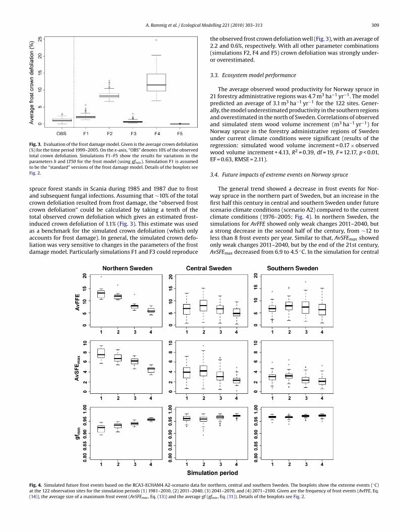
Fig. 3. Evaluation of the frost damage model. Given is the average crown defoliation(%) for the time period 1999–2005. On the x-axis, “OBS” denotes 10% of the observedtptF

sacctiaald

Fa(

otal crown defoliation. Simulations F1–F5 show the results for variations in thearameters b and LT50 for the frost model (using gfmin). Simulation F1 is assumedo be the “standard” versions of the frost damage model. Details of the boxplots seeig. 2.

pruce forest stands in Scania during 1985 and 1987 due to frostnd subsequent fungal infections. Assuming that ∼10% of the totalrown defoliation resulted from frost damage, the “observed frostrown defoliation” could be calculated by taking a tenth of theotal observed crown defoliation which gives an estimated frost-

nduced crown defoliation of 1.1% (Fig. 3). This estimate was useds a benchmark for the simulated crown defoliation (which onlyccounts for frost damage). In general, the simulated crown defo-iation was very sensitive to changes in the parameters of the frostamage model. Particularly simulations F1 and F3 could reproduce

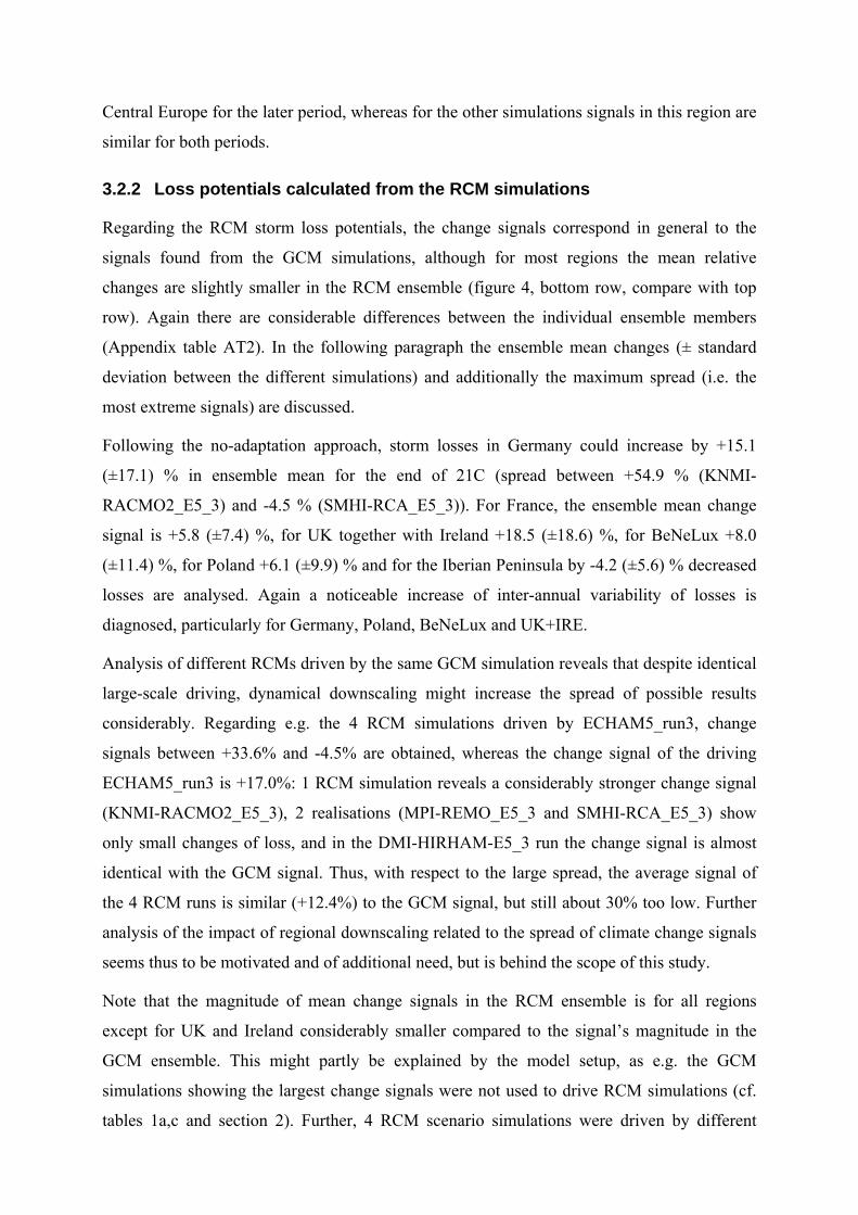
ig. 4. Simulated future frost events based on the RCA3-ECHAM4 A2-scenario data for nt the 122 observation sites for the simulation periods (1) 1981–2010, (2) 2011–2040, (3)14)), the average size of a maximum frost event (AvSFEmax , Eq. (13)) and the average gf (g

elling 221 (2010) 303–313 309

the observed frost crown defoliation well (Fig. 3), with an average of2.2 and 0.6%, respectively. With all other parameter combinations(simulations F2, F4 and F5) crown defoliation was strongly under-or overestimated.

3.3. Ecosystem model performance

The average observed wood productivity for Norway spruce in21 forestry administrative regions was 4.7 m3 ha−1 yr−1. The modelpredicted an average of 3.1 m3 ha−1 yr−1 for the 122 sites. Gener-ally, the model underestimated productivity in the southern regionsand overestimated in the north of Sweden. Correlations of observedand simulated stem wood volume increment (m3 ha−1 yr−1) forNorway spruce in the forestry administrative regions of Swedenunder current climate conditions were significant (results of theregression: simulated wood volume increment = 0.17 × observedwood volume increment + 4.13, R2 = 0.39, df = 19, F = 12.17, p < 0.01,EF = 0.63, RMSE = 2.11).

3.4. Future impacts of extreme events on Norway spruce

The general trend showed a decrease in frost events for Nor-way spruce in the northern part of Sweden, but an increase in thefirst half this century in central and southern Sweden under futurescenario climate conditions (scenario A2) compared to the currentclimate conditions (1976–2005; Fig. 4). In northern Sweden, the

simulations for AvFFE showed only weak changes 2011–2040, buta strong decrease in the second half of the century, from ∼12 toless than 8 frost events per year. Similar to that, AvSFEmax showedonly weak changes 2011–2040, but by the end of the 21st century,AvSFEmax decreased from 6.9 to 4.5 ◦C. In the simulation for central

orthern, central and southern Sweden. The boxplots show the extreme events (◦C)2041–2070, and (4) 2071–2100. Given are the frequency of frost events (AvFFE, Eq.fmin , Eq. (11)). Details of the boxplots see Fig. 2.

310 A. Rammig et al. / Ecological Modelling 221 (2010) 303–313

Table 4Evaluation of simulation results under future climate conditions (RCA3/ECHAM4/A2). The %-values in A) give the relative change of simulations where frost damage wasincluded in comparison to “No frost”-simulations.

(A) Average stem wood volume (m3 ha−1)a (B) Percentage of increase relative to 1976–2005 (%)

1976–2005 1981–2010 2011–2040 2041–2070 2071–2100 1981–2010 2011–2040 2041–2070 2071–2100

S. SwedenNo frost (FNO) 219.5 219.8 232.6 253.2 265.4 0.2 6.0 15.4 20.9Frost (F1) 207.3 207.4 220.2 241.9 255.2 0.1 6.2 16.7 23.1

−5.5% −5.6% −5.3% −4.5% −3.8%

C. SwedenNo frost (FNO) 221.0 222.9 241.2 262.4 276.8 0.9 9.1 18.7 25.2Frost (F1) 205.5 206.6 221.6 244.8 262.6 0.5 7.9 19.1 27.8

−7.0% −7.3% −8.1% −6.7% −5.1%

N. SwedenNo frost (FNO) 137.0 137.5 147.8 163.6 169.7 0.4 7.8 19.4 23.8Frost (F1) 102.0 102.5 123.0 140.3 149.3 0.4 20.5 37.5 46.3

nd agea f 740 t

aS3fpfsdtfId

3

sdadaf

a(mpd

cvmnsfdts(

4

saa

−25.5% −25.5% −16.8% −14.2%

a Norway spruce stands were prescribed in the simulations to have the same stage was on average 69 years (Stdev: 12, min: 36, max: 95) and an average density o

nd southern Sweden, a different pattern was observed. In centralweden, AvFFE increased from 6 to 8 and AvSFEmax increased from.9 to 4.6 ◦C in the first half of the century. In southern Sweden, therequency of frost events (AvFFE) increased for a longer transienteriod until 2071. In the end of the 21st century, the frequency of

rost events (AvFFE) decreased to 5 in central and 6 frost events inouthern Sweden. The average maximum frost events (AvSFEmax)ecreased to 2.4 and 2.1 ◦C, respectively. The growth reducing fac-or (gfmin) varies according to AvSFEmax (Fig. 4). In northern Sweden,rost events have less impact on growth by the end of the century.n central Sweden, there is a transient period with increased frostamage during the first half of the century (Fig. 4).

.5. Forest productivity under future climate conditions

In general, all model versions projected an increase in Norwaypruce stand wood volume under the SRES-A2 future climate con-itions for all regions in Sweden (Table 4A). The model projectedn increase in mean annual stem wood volume in southern Swe-en from 219 to 265 m3 ha−1 for the period 1976–2100. In centralnd northern Sweden, stem wood volume was projected to increaserom 221 to 277 m3 ha−1, and from 137 to 170 m3 ha−1, respectively.

Simulated stem wood volume of Norway spruce was gener-lly lower if frost damage was included in the ecosystem modelTable 4A). In southern Sweden, when including frost damage, the

odel projected ∼5% less stem wood volume for 1976–2100 in com-arison to the FNO-simulations. For this period, stem volume wasecreased by ∼7% in central and 19% in northern Sweden.

The percentage of increase in stem wood volume under futurelimate conditions relative to 1976–2005 was positive for all modelersions (Table 4B). Under current conditions, frost damages areore important than under future climate conditions. A higher

umber of frost damages lowered the productivity in the F1-imulations under current conditions. Under future conditions,rost damage is occurring less frequently, leading to a higher pro-uctivity in the F1-simulations relative to 1976–2005 and relativeo the FNO-simulations. The increase of wood volume in the F1-imulations was projected to be 23% (south), 28% (central) and 46%north) for 2071–2100 relative to 1976–2005.

. Discussion

Seasonal variations in physiological processes in plants aretrongly driven by climate variables such as temperature and watervailability (Lambers et al., 2000). Climate change can thereforeffect such processes. The risk of future weather events exceeding

−12.0%

and density as the observed sites. At the end of each simulation period, the standrees ha−1 (Stdev: 269, min: 111, max: 1147).

the physiological tolerance of different species and thus causingdamage and reduced functioning can be explored by driving mod-els that encapsulate the relevant processes with data from climatescenarios. Ours is an example of such a study for the case of frostdamage in boreal forests. The hardiness model used (Jönsson et al.,2004) includes the gradual change in the environmental responseof frost hardiness. It considers the effect of both temperature andphotoperiod on the level of frost hardiness. In combination withthe frost damage model, frost damage in autumn, mid-winter andspring are considered.

We found a strong decrease of frost events in northern and onlylittle changes in central and southern Sweden under the futureclimate scenario investigated. Results from Jönsson et al. (2004)indicated latitudinal differences in the risk for frost, with a highnumber of spring frost events and almost no autumn frost events inthe South of Sweden for the period 1961–1990. In northern Sweden,their simulations showed opposite results: a low number of springfrost, but a high number of autumn frost events. Using data for theIPCC A2 and B2 future climate scenario for the period of 2070–2099from another combination of global and regional climate models,i.e. data from the Hadley Centre regional climate model HadRM3H,their model simulations showed a marked increase in the num-ber of spring frost events in the south and a decreased numberof autumn frost events in the north of Sweden. We did not dis-tinguish between spring and autumn frost events in the presentstudy; the results do not reflect an increase of spring frost eventsdue to a simultaneous decrease in autumn frost events (results notshown). Interestingly, our results suggest an increase in frost eventsin southern Sweden during the period 2011–2040, while simulatedfrost events strongly decreased in Sweden 2041–2100. This sug-gests that the increased risk for damage may not be permanentbut a temporary effect of increased risk for frost damage during atransient period caused by premature dehardening and therefore ahigher probability of temperature backlashes below freezing. Witha further increase in winter temperatures, the risk for frost dam-age could be reduced. The frequency and severity of harmful frostevents will change over time, but trajectories may vary depend-ing on climate scenarios. Data from another combination of globaland regional climate models, or from the same model forced by adifferent GHG emissions scenario, may result in a differently mod-elled frost damage. With a lower temperature increase, e.g. under

the SRES B1 and B2 scenarios (Nakicenovic et al., 2000), the risk forfrost damage could be elevated for a longer period of time. In thediscussion of options to reduce the risk of frost-related damages,such as by the adaptive selection of species and provenances, it isnecessary to consider the outcome of a range of contrasting climate

l Mod

cz(

fiepeffofrNiatess

waiH2d1eFaovstmafcBsit

(mwCiertacmelpoigmWpsr

A. Rammig et al. / Ecologica

hange scenarios in relation to species-specific ability for acclimati-ation, local adaptation and genetic adaptation by natural selectionHänninen et al., 2001; Jönsson et al., 2004).

To introduce the effect of frost events into the ecosystem model,rst, a “growth reducing factor” (gf) was calculated after Kellomäkit al. (1995) and Leinonen (1996). Their frost damage model wasarameterised for Scots pine (P. sylvestris), but resulted in appar-ntly realistic estimates for crown defoliation in our simulationsor Norway spruce. However, both the observed and simulatedrost crown defoliation are uncertain. We estimated that 6–12%f the total observed crown defoliation may be associated withrost events (Fig. 3). This is within the same range as valueseported from monitoring observations in southern Sweden (e.g.ihlgård, 1990), but crown defoliation of a stand is additionally

nfluenced by latitude, stand age, precipitation and nitrogen avail-bility (Rosengren-Brinck, 1998). However, the correlation betweenhe simulated frost damage and crown defoliation is unlikely to bexplained by covariance with these variables: frost events were notignificantly correlated with stand age and soil water (results nothown). Nitrogen dynamics were not explicitly addressed.

Sensitivity analysis showed that the simulated crown defoliationas very sensitive to changes in the parameters of the frost dam-

ge model. While much effort has been put into evaluating andmproving parameters for various models of frost hardiness (e.g.annerz and Westin, 2005; Hänninen, 2006; Hänninen and Kramer,007), parameters for estimating the actual frost damage on nee-les or whole forests have rarely been derived (but see Leinonen,996; Leinonen et al., 1997). Observations of damage to whole for-st stands have been made in the U.S.A. (Hagle et al., 2003) andinland (Jalkanen and Närhi, 1992; Jalkanen, 1996), where temper-ture inversions on mountain slopes damage large forest areas. Inur study, the simulated crown defoliation resembled the naturalariation and the amount of frost crown defoliation best when thetandard parameters were used for the calculation of growth reduc-ion (Table 3, simulation F1; Fig. 3). This suggests that simulated

aximum frost events (largest difference between hardiness levelnd daily minimum temperature) are best predictors for potentialrost damages. Such events are likely to be particularly sensitive tohanges in the seasonality and variability in daily temperatures (e.g.igras and Colombo, 2000; IPCC, 2007; Woldendorp et al., 2008),uggesting that impact modelling, such as projecting frost damagento the future, requires improved climate data at high spatial andemporal resolution.

Our study takes advantage of the high temporal resolution30 min; see Section 2) of data generated by the regional climate

odel RCA3. The input to the ecosystem model thus reflected dailyeather variations including the diurnal cycle in a realistic way.ompared with monthly mean data as used in many previous stud-

es of regional vegetation changes (e.g. Koca et al., 2006; Moralest al., 2007), this enables more realistic simulation of non-linearesponses of physiological processes to variable weather condi-ions, including extremes. However, in the context of many plantnd ecosystem processes, the spatial resolution of the RCM is ratheroarse. In reality, each simulated 50 km × 50 km gridcell containsany different vegetation stands and landscape units that influ-

nce local climate via variation in topography, hydrology, roughnessength and surface exchange. This heterogeneity is absent or highlyarameterised in the RCM which merely distinguishes the fractionsf ‘open land’ and ‘forest’ (Samuelsson et al., 2006). The variation

n local climate conditions this results in is aggregated to a sin-le value for each grid cell. The coarser the grid resolution, the

ore smoothed the simulated climate will be in terms of extremes.hile the spatial resolution of RCMs are steadily improved in

arallel with introduction of more sophisticated land-surfacechemes, the need for gridcell-to-point (site) downscaling willemain.

elling 221 (2010) 303–313 311

LPJ-GUESS has been shown to reproduce observed variations inecosystem productivity along broad climatic gradients (Morales etal., 2005; Zaehle et al., 2006) such as in Fennoscandia (Koca et al.,2006; Smith et al., 2008) and in response to elevated CO2 (Hickler etal., 2008). LPJ-GUESS is a generalised model which is not expected touniformly reproduce site-specific productivity because it does notinclude site-specific information such as detailed soil propertiesand scaling parameters for plant physiological processes as inputdata, as such data are not available for spatially extensive (grid-based) studies. One result of the generalised parameterisation wasthat the model underestimated productivity in the south of Swedenand overestimated it in the north. In addition, nutrient limitations,which are regarded as significant in the northern boreal forest, arenot included in the model. Bias in the simulated productivity gra-dient is, however, not critical for the effects of frost damage. Underfutures climate conditions, our simulation results suggest a strongincrease in the total productivity of Norway spruce stands (Table 4).However, including the physiological process of hardening and thesubsequent risk of frost damage by reducing the growth of the trees,the model projects lower productivity. Our simulation results sug-gest that frost events reduce stand productivity much more stronglyunder current climate conditions (i.e. 5% in the south and 25% inthe north of Sweden) than might be expected under an A2 futureclimate scenario (i.e. only 4% in the south and 12% in the north;Table 4). However, this reduction in productivity may be under-estimated, since the growth reducing effect of frost damage, wasonly calculated once per year in LPJ-GUESS, frost events were aggre-gated from among seasons into one value. In reality, there are oftenlarge differences in damage potential between spring and autumnfrost events. During spring, new buds and shoots are very sensi-tive to frost, whereas older shoots are more tolerant (Cannell andSheppard, 1982; Bigras and Colombo, 2000).

Our results point to the importance of including representationsof hardening/dehardening cycles and frost damage in ecosystemmodels to correctly capture transient changes in productivity andcarbon cycling of high-latitude forest ecosystems under globalchange.

Acknowledgements

The Project “Climate extremes & Ecosystem modelling” wasfunded by the Swedish Research Council. Part of this work was donewithin the EU/FP6 ENSEMBLES project (GOCE-CT-2003-505539).

Appendix A. Supplementary data

Supplementary data associated with this article can be found, inthe online version, at doi:10.1016/j.ecolmodel.2009.05.014.

References

Alden, J., Hermann, R.K., 1971. Aspects of the cold-hardiness mechanism in plants.Botanical Review 37, 37–142.

Badeck, F.-W., Lischke, H., Bugmann, H., et al., 2001. Tree species composition in Euro-pean pristine forests. Comparison of stand data to model predictions. ClimaticChange 51, 307–347.

Bartelink, H.H., 2000. Effects of stand composition and thinning in mixed-speciesforests: a modeling approach applied to Douglas-fir and beech. Tree Physiology20, 399–406.

Bergh, J., Freeman, M., Sigurdsson, B., et al., 2003. Modelling the short-term effects ofclimate change on the productivity of selected tree species in Nordic countries.Forest Ecology and Management 183, 327–340.

Bigras, F.J., Colombo, S.J., 2000. Conifer Cold Hardiness. Kluwer Academic, Boston,596 pp.

Bonan, G.B., Shugart, H.H., 1989. Environmental factors and ecological processes inboreal forests. Annual Review of Ecology and Systematics 20, 1–28.

Burr, K.E., Hawkins, C.D.B., Hirondelle, S.J.L., Binder, W.D., George, M.F., Repo, T.,2001. Methods for measuring cold hardiness of conifers. In: Bigras, F.J., Colombo,S.J. (Eds.), Conifer Cold Hardiness. Kluwer Academic Publishers, Dordrecht, pp.369–401.

3 l Mod

B

C

C

C

C

E

F

H

H

H

H

H

H

H

H

H

H

I

J

J

J

J

J

J

J

J

J

12 A. Rammig et al. / Ecologica

ugmann, H., 1994. On the ecology of mountainous forests in a changing climate:a simulation study. Ph.D. Thesis. Swiss Federal Institute of Technology Zurich,Zurich, 258 pp.

annell, M.G.R., Sheppard, L.J., 1982. Seasonal changes in the frost hardiness of prove-nances of Picea sitchensis in Scotland. Forestry 55, 137–153.

annell, M.G.R., Smith, R.I., 1986. Climatic warming, spring budburst and forest dam-age on trees. Journal of Applied Ecology 23 (1), 177–191.

hen, H.-H., Li, P.H., 1978. Interactions of low temperature, water stress and shortdays in the induction of stem frost hardiness in red osier dogwood. Plant Physi-ology 62, 833–835.

hristensen, J.H., Hewitson, B., Busuioc, A., et al., 2007. Regional climate projections.In: Solomon, S., Qin, D., Manning, M., Chen, Z., Marquis, M., Averyt, K.B., Tignor, M.,Miller, H.L. (Eds.), Climate Change 2007: The Physical Science Basis. Contributionof Working Group I to the Fourth Assessment Report of the IntergovernmentalPanel on Climate Change. Cambridge University Press, pp. 847–940.

ichhorn, J., Szepesi, A., Ferretti, M., Durrant, D., Roskams, P., 2006. Manual on meth-ods and criteria for harmonized sampling, assessment, monitoring and analysisof the effects of air pollution on forests, Part II: visual assessment of crowncondition. In: ICP Forests Manual. United Nations Economic Commission forEurope, Convention on Long-Range Transboundary Air Pollution, InternationalCo-operative Programme on Assessment and Monitoring of Air Pollution Effectson Forests, Hamburg, Germany.

uchigami, L.H., Weiser, C.J., Kobayashi, K., Timmis, R., Gusta, L.V., 1982. A degreegrowth stage (◦GS) model and cold acclimation in temperate woody plants. In:Li, P.H., Sakai, A. (Eds.), Plant Cold Hardiness and Freezing Stress. Mechanismsand Crop Implications. Academic Press, New York, pp. 93–116.

äggmark, L., Ivarsson, K.-I., Olofsson, P.-O., Gollvik, S., 2000. Mesan, an operationalmesoscale analysis system. Tellus 52A, 2–20.

agle, S.K., Gibson, K.E., Tunnock, S., 2003. A Field Guide to Diseases and Insect Pestsof Northern and Central Rocky Mountain Conifers. United States Department ofAgriculture, Forest Service, Missoula, Montana.

annerz, M., 1994. Predicting the risk of frost occurrence after bud burst of Norwayspruce in Sweden. Silva Fennica 28, 243–249.

annerz, M., Westin, J., 2005. Autumn frost hardiness in Norway spruce plus treeprogeny and trees of the local and transferred provenances in central Sweden.Tree Physiology 25, 1181–1186.

änninen, H., 2006. Climate warming and the risk of frost damage to boreal for-est trees: identification of critical ecophysiological traits. Tree Physiology 26,889–898.

änninen, H., Beuker, E., Johnsen, O., Leinonen, I., Murray, M., Sheppard, L., Skroppa,T., 2001. Impacts of climate change on cold hardiness of conifers. In: Bigras,F.J., Colombo, S.J. (Eds.), Conifer Cold Hardiness. Kluwer Academic, Boston, pp.305–333.

änninen, H., Kramer, K., 2007. A framework for modelling the annual cycle of treesin boreal and temperate regions. Silva Fennica 41 (1), 167–205.

arrison, L.C., Weiser, C.J., Burke, M.J., 1978. Environmental and seasonal factorsaffecting the frost-induced stage of cold acclimation in Cornus stolonifera Michx.Plant Physiology 62, 894–898.

ickler, T., Smith, B., Sykes, M.T., Davis, M.B., Sugita, S., Walker, K., 2004. Using ageneralized vegetation model to simulate vegetation dynamics in northeasternUSA. Ecology 85 (2), 519–530.

ickler, T., Smith, B., Prentice, I.C., Mjöfors, K., Miller, P., Arneth, A., Sykes, M., 2008.CO2 fertilization in temperate FACE experiments not representative of borealand tropical forests. Global Change Biology 14, 1531–1542.

PCC, 2007. Climate Change 2007: The Physical Science Basis. Contribution of Work-ing Group I to the Fourth Assessment Report of the Intergovernmental Panel onClimate Change. Cambridge University Press, Cambridge, United Kingdom andNew York, NY, USA, 996 pp.

aakkola, T., Mäkinen, H., Saranpää, P., 2006. Wood density of Norway spruce:responses to timing and intensity of first commercial thinning and fertilisation.Forest Ecology & Management 237, 513–521.

acob, D., Barring, L., Christensen, O.B., Christensen, J.H., de Castro, M., Deque, M.,Giorgi, F., Hagemann, S., Lenderink, G., Rockel, B., Sanchez, E., Schar, C., Senevi-ratne, S.I., Somot, S., van Ulden, A., van den Hurk, B., 2007. An inter-comparison ofregional climate models for Europe: model performance in present-day climate.Climatic Change 81, 31–52.

alkanen, R., 1996. Repeated red belts at Lusmavaara, western Lapland. Pallas-Symposium 1996. Finnish Forest Research Institute, Research Papers 623, 91–95.

alkanen, R., Närhi P., 1992. Red Belt Phenomenon on the Slopes of the Levi fell inKittilä, Western Lapland. The Finnish Forest Research Institute, Research Papers,vol. 451, pp. 55–60.

ansson, A., Persson, C., Strandberg, G., 2007. 2D meso-scale re-analysis of precipita-tion, temperature and wind over Europe–ERAMESAN, Time period 1980–2004.SMHI Reports Meteorology and Climatology, No. 112, 28 pp.

arvis, P., Saugier, B., Schulze, E.-D., 2001. Productivity of boreal forests. In: Roy, J.,Saugier, B., Mooney, H.A. (Eds.), Terrestrial Global Productivity. Academic Press,San Diego, London, pp. 211–244.

önsson, A.M., Linderson, M.-L., Stjernquist, I., Schlyter, P., Bärring, L., 2004. Climatechange and the effect of temperature backlashes causing frost damage in Piceaabies. Global and Planetary Change 44, 195–207.

önsson, A.M., 2005. Tracing the impact of adverse environmental conditions on thefrost sensitivity in trees. Journal of Sustainable Forestry 21, 65–75.

oos, F., Prentice, I.C., Sitch, S., Meyer, R., Hooss, G., Plattner, G.K., Gerber, S., Hassel-mann, K., 2001. Global warming feedbacks on terrestrial carbon uptake under theIntergovernmental Panel on Climate Change (IPCC) emission scenarios. GlobalBiogeochemical Cycles 15, 891–907.

elling 221 (2010) 303–313

Karlman, M., 1986. Damage to Pinus contorta in northern Sweden with specialemphasis on pathogens. Stud. For. Sue, No. 176. Faculty of Forestry, SwedishUniv. of Agricultural Sciences, Uppsala, 42 pp.

Kellomäki, S., Hänninen, H., Kolström, M., 1995. Computations on frost damage toScots pine under climatic warming in boreal conditions. Ecological Applications5 (1), 42–52.

Kjellström, E., 2004. Recent and future signatures of climate change in Europe. Ambio33, 193–198.

Kjellström, E., Bärring, L., Gollvik, S., Hansson, U., Jones, C., Samuelsson, P., Rum-mukainen, M., Ullerstig, A., Willén, U., Wyser, K., 2005. A 140-year simulationof European climate with the new version of the Rossby Centre regional atmo-spheric climate model (RCA3). SMHI Reports Meteorology and Climatology 108,1–54.

Kjellström, E., Bärring, L., Jacob, D., Jones, R., Lenderink, G., Schär, C., 2007. Modellingdaily temperature extremes: recent climate and future changes over Europe.Climatic Change 81 (Suppl. 1), 249–265.

Koca, D., Smith, B., Sykes, M., 2006. Modelling regional climate change effects onpotential natural ecosystems in Sweden. Climatic Change 78, 381–406.

Köstler, J.N., Brückner, E., Biebelriether, H., 1968. Die Wurzeln der Waldbäume. PaulParey, Hamburg, 284 pp.

Köstner, B., Falge, E., Tenhunen, J.D., 2002. Age-related effects on leaf area/sapwoodarea relationships, canopy transpiration and carbon gain of Norway sprucestands (Picea abies) in the Fichtelgebirge, Germany. Tree Physiology 22, 567–574.

Kowalski, T., 1991. Oak decline: I. Fungi associated with various disease symptomson overground portions of middle-aged and old oak (Quercus robur L.). EuropeanJournal of Forest Pathology, 21.

Kowalski, T., 1996. Oak decline: II. Fungi associated with various types of lesions onstems and branches of young oaks (Quercus robur L.). Österr. Z. Pilzk. 5, 51–63.

Lambers, H., Chapin, F.S., Pons, T.L., 2000. Plant Physiological Ecology. Springer Ver-lag, New York, Berlin, Heidelberg, 540 pp.

Leinonen, I., 1996. A simulation model for the annual frost hardiness and freezedamage of Scots pine. Annals of Botany 78, 687–693.

Leinonen, I., Repo, T., Hänninen, H., 1997. Changing environmental effects onfrost hardiness of Scots pine during dehardening. Annals of Botany 79, 133–138.

Li, Z., Kurz, W.A., Apps, M.J., Beukema, S.J., 2003. Belowground biomass dynamics inthe Carbon Budget Model of the Canadian Forest Sector: recent improvementsand implications for the estimation of NPP and NEP. Canadian Journal of ForestResearch 33, 106–126.

Linder, S., Flower-Ellis, J.G.K., 1992. Environmental and physiological constraints toforest yield. In: Teller, A., Mathy, P., Jeffers, J.N.R. (Eds.), Responses of ForestEcosystems to Environmental Changes. Elsevier Applied Science, London, pp.149–164.

Mayer, D.G., Butler, D.G., 1993. Statistical validation. Ecological Modelling 68, 21–32.Morales, P., Sykes, M.T., Prentice, I.C., et al., 2005. Comparing and evaluating

process-based ecosystem model predictions of carbon and water fluxes in majorEuropean forest biomes. Global Change Biology 11, 2211–2233.

Morales, P., Hickler, T., Rowell, D., Smith, B., Sykes, M., 2007. Changes in Europeanecosystem productivity and carbon balance driven by regional climate modeloutput. Global Change Biology 13, 108–122.

Nakicenovic, N., Alcamo, J., Davis, G., et al., 2000. IPCC Special Report on EmissionScenarios. Cambridge University Press, Cambridge, 612 pp.

Nihlgård, B., 1990. Dynamik i barrkemi och barrstrukturer på Skånska gran-och tall-provytor åren 1985–1987. Skånes samrådesgrupp mot skogsskador Rapport, Nr.8, 91 pp.

Niinemets, Ü., Lukjanova, A., 2003. Total foliar area and average leaf age may bemore strongly associated with branching frequency than with leaf longevity intemperate conifers. New Phytologist 158, 75–89.

Ögren, E., 2001. Effects of climatic warming on cold hardiness of some northernwoody plants assessed from simulation experiments. Physiologia Plantarum 112,71–77.

Prentice, I.C., Sykes, M.T., Cramer, W., 1993. A simulation model for the transienteffects of climate change on forest landscapes. Ecological Modelling 65, 51–70.

Repo, T., Hänninen, H., Kellomäki, S., 1996. The effects of long-term elevation ofair temperature and CO2 on the frost hardiness of Scots pine. Plant, Cell andEnvironment 19, 209–216.

Roeckner, E., Bengtsson, L., Feichter, J., Lelieveld, J., Rodhe, H., 1999. Transient cli-mate change simulations with a coupled atmosphere-ocean GCM including thetropospheric sulfur cycle. Journal of Climate 12, 3004–3032.

Rosengren-Brinck, U., 1998. Barrförlust och luftföroreningar: Samband mellan kro-nutglesning och miljöfaktorer I barrskog. Naturvårdsverket Rapport, 4890 pp.

Sakai, A., Larcher, W., 1987. Frost Survival of Plants. Springer Verlag, Berlin, Germany,321 pp.

Saltelli, A., Chan, K., Scott, E.M., 2000. Sensitivity Analysis. John Wiley & Sons, Ltd.,Chichester, New York, Weinheim, 475 pp.

Samuelsson, P., Gollvik, S., Ullerstig, A., 2006. The land-surface scheme of the RossbyCentre regional atmospheric climate model (RCA3). SMHI Rapport Meteorologi,Nr. 122, 25 pp.

Schoeneweiss, D.F., 1975. Predisposition, stress and plant disease. In: Baker-Kenneth,F. (Ed.), Annual Review of Phytopathology. Illus Annual Reviews, Palo Alto, CA,

USA, pp. 193–211.

Sieber, T.N., Kowalski, T., Holdenrieder, O., 1995. Fungal assemblages in stem andtwig lesions of Quercus robur in Switzerland. Mycological Research 99, 534–538.

Sitch, S., Smith, B., Prentice, I.C., Arneth, A., Bondeau, A., Cramer, W., Kaplans, J.O.,Levis, S., Lucht, W., Sykes, M.T., Thonicke, K., Venevsky, S., 2003. Evaluation of

l Mod

S

S

S

S

U

and ecosystem functioning in European forest biomes. Ecological Modelling 216,

A. Rammig et al. / Ecologica

ecosystem dynamics, plant geography and terrestrial carbon cycling in the LPJdynamic global vegetation model. Global Change Biology 9, 161–185.

mith, B., Knorr, W., Widlowski, J.L., Pinty, B., Gobron, N., 2008. Combining remotesensing data with process modelling to monitor boreal conifer forest carbonbalances. Forest Ecology & Management 255, 3985–3994.

mith, B., Prentice, I.C., Sykes, M., 2001. Representation of vegetation dynamics inthe modelling of terrestrial ecosystems: comparing two contrasting approacheswithin European climate space. Global Ecology and Biogeography 10, 621–637.

utinen, M.-L., Arora, R., Wisniewski, M., Ashworth, E., Strimbeck, R., Palta, J.P.,2001. Mechanisms of frost survival and freeze-damage in nature. In: Bigras,

F.J., Colombo, S.J. (Eds.), Conifer Cold Hardiness. Kluwer Academic Publishers,Dordrecht, pp. 89–120.

wedish Forest Agency, 2007. Statistical Yearbook of Forestry 2007. Skogsstyrelsen,Jönköping, Sweden, 345 pp.

ppala, S.M., Kållberg, P.W., Simmons, A.J., et al., 2005. The ERA-40 re-analysis. Quar-terly Journal of the Royal Meteorological Society 131, 2961–3012.

elling 221 (2010) 303–313 313

Vogt, K.A., Vogt, D.J., Palmiotto, P.A., Boon, P., O’Hara, J., Asbjörnson, H., 1996. Reviewof root dynamics in forest ecosystems grouped by climate, climatic forest typeand species. Plant and Soil 187, 159–219.

Woldendorp, G., Hill, M.J., Doran, R., Ball, M.C., 2008. Frost in a future climate: mod-elling interactive effects of warmer temperatures and rising atmospheric [CO2]on the incidence and severity of frost damage in a temperate evergreen (Euca-lyptus pauciflora). Global Change Biology 14, 294–308.

Wramneby, A., Smith, B., Zaehle, S., Sykes, M.T., 2008. Parameter uncertainties inthe modelling of vegetation dynamics—effects on tree community structure

277–290.Zaehle, S., Sitch, S., Prentice, I.C., Liski, J., Cramer, W., Erhard, M., Hickler, T.,

Smith, B., 2006. The importance of representing age-related decline in forestNPP for modeling regional carbon balances. Ecological Applications 16, 1555–1574.