Projections of Future Climate Change -...

Projections of Future Climate Change

Co-ordinating Lead AuthorsU. Cubasch, G.A. Meehl

Lead AuthorsG.J. Boer, R.J. Stouffer, M. Dix, A. Noda, C.A. Senior, S. Raper, K.S. Yap

Contributing AuthorsA. Abe-Ouchi, S. Brinkop, M. Claussen, M. Collins, J. Evans, I. Fischer-Bruns, G. Flato, J.C. Fyfe,A. Ganopolski, J.M. Gregory, Z.-Z. Hu, F. Joos, T. Knutson, R. Knutti, C. Landsea, L. Mearns, C. Milly,J.F.B. Mitchell, T. Nozawa, H. Paeth, J. Räisänen, R. Sausen, S. Smith, T. Stocker, A. Timmermann,U. Ulbrich, A. Weaver, J. Wegner, P. Whetton, T. Wigley, M. Winton, F. Zwiers

Review EditorsJ.-W. Kim, J. Stone

9

Contents

Executive Summary 527

9.1 Introduction 5309.1.1 Background and Recap of Previous Reports 5309.1.2 New Types of Model Experiments since

1995 531

9.2 Climate and Climate Change 5329.2.1 Climate Forcing and Climate Response 5329.2.2 Simulating Forced Climate Change 534

9.2.2.1 Signal versus noise 5349.2.2.2 Ensembles and averaging 5349.2.2.3 Multi-model ensembles 5359.2.2.4 Uncertainty 536

9.3 Projections of Climate Change 5369.3.1 Global Mean Response 536

9.3.1.1 1%/yr CO2 increase (CMIP2) experiments 537

9.3.1.2 Projections of future climate from forcing scenario experiments (IS92a) 541

9.3.1.3 Marker scenario experiments (SRES) 541

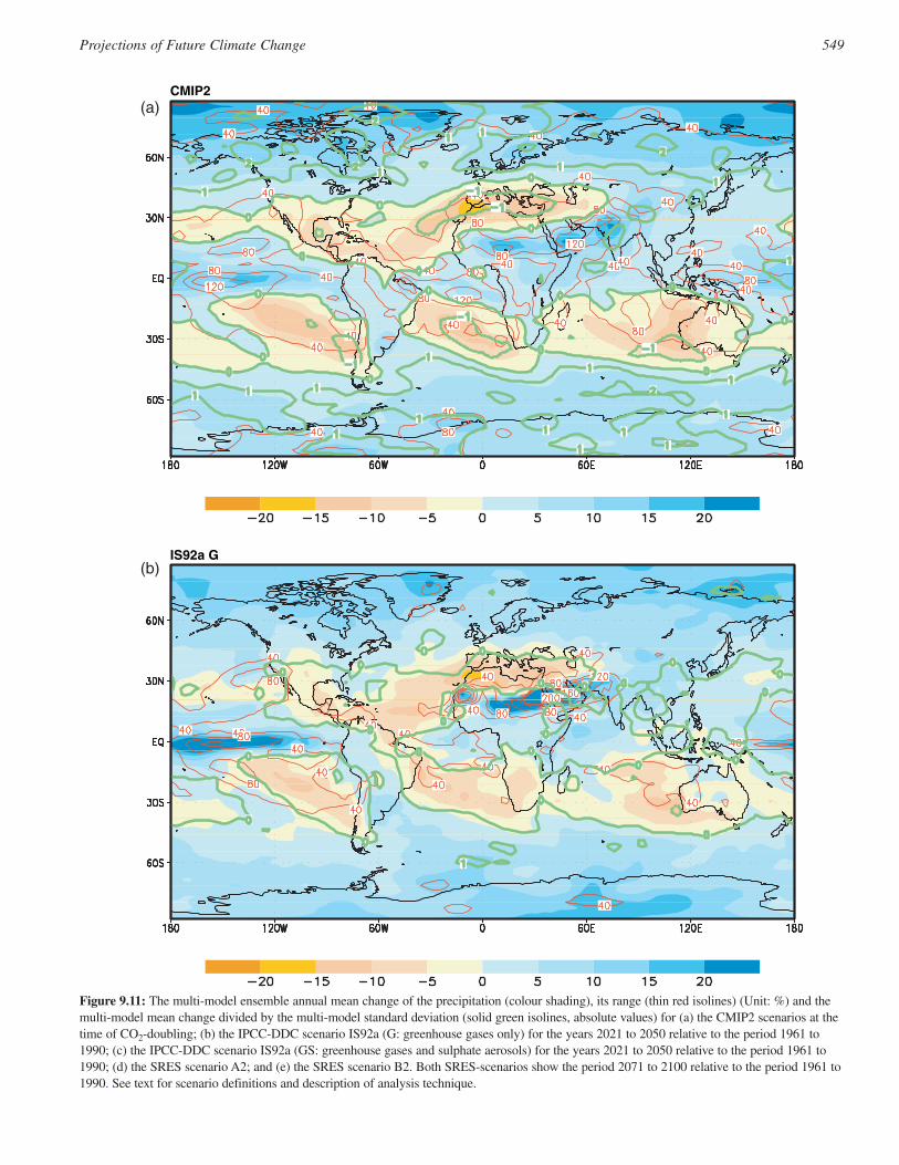
9.3.2 Patterns of Future Climate Change 5439.3.2.1 Summary 548

9.3.3 Range of Temperature Response to SRESEmission Scenarios 554

9.3.3.1 Implications for temperature of stabilisation of greenhouse gases 557

9.3.4 Factors that Contribute to the Response 5599.3.4.1 Climate sensitivity 5599.3.4.2 The role of climate sensitivity and

ocean heat uptake 5619.3.4.3 Thermohaline circulation changes 5629.3.4.4 Time-scales of response 563

9.3.5 Changes in Variability 5659.3.5.1 Intra-seasonal variability 5669.3.5.2 Interannual variability 5679.3.5.3 Decadal and longer time-scale

variability 5689.3.5.4 Summary 570

9.3.6 Changes of Extreme Events 5709.3.6.1 Temperature 5709.3.6.2 Precipitation and convection 5729.3.6.3 Extra-tropical storms 5739.3.6.4 Tropical cyclones 5749.3.6.5 Commentary on changes in

extremes of weather and climate 5749.3.6.6 Conclusions 575

9.4 General Summary 576

Appendix 9.1: Tuning of a Simple Climate Model toAOGCM Results 577

References 578

527Projections of Future Climate Change

Executive Summary

The results presented in this chapter are based on simulationsmade with global climate models and apply to spacial scales ofhundreds of kilometres and larger. Chapter 10 presents results forregional models which operate on smaller spatial scales. Climatechange simulations are assessed for the period 1990 to 2100 andare based on a range of scenarios for projected changes ingreenhouse gas concentrations and sulphate aerosol loadings(direct effect). A few Atmosphere-Ocean General CirculationModel (AOGCM) simulations include the effects of ozone and/orindirect effects of aerosols (see Table 9.1 for details). Mostintegrations1 do not include the less dominant or less wellunderstood forcings such as land-use changes, mineral dust,black carbon, etc. (see Chapter 6). No AOGCM simulationsinclude estimates of future changes in solar forcing or in volcanicaerosol concentrations.

There are many more AOGCM projections of future climateavailable than was the case for the IPCC Second AssessmentReport (IPCC, 1996) (hereafter SAR). We concentrate on theIS92a and draft SRES A2 and B2 scenarios. Some indication ofuncertainty in the projections can be obtained by comparing theresponses among models. The range and ensemble standarddeviation are used as a measure of uncertainty in modelledresponse. The simulations are a combination of a forced climatechange component together with internally generated naturalvariability. A number of modelling groups have producedensembles of simulations where the projected forcing is the samebut where variations in initial conditions result in differentevolutions of the natural variability. Averaging these integrationspreserves the forced climate change signal while averaging out thenatural variability noise, and so gives a better estimate of themodels’ projected climate change.

For the AOGCM experiments, the mean change and therange in global average surface air temperature (SAT) for the1961 to 1990 average to the mid-21st century (2021 to 2050) forIS92a is +1.3°C with a range from +0.8 to +1.7°C for greenhousegas plus sulphates (GS) as opposed to +1.6°C with a range from+1.0 to +2.1°C for greenhouse gas only (G). For SRES A2 themean is +1.1°C with a range from +0.5 to +1.4°C, and for B2, themean is +1.2°C with a range from +0.5 to +1.7°C.

For the end of the 21st century (2071 to 2100), for the draftSRES marker scenario A2, the global average SAT change fromAOGCMs compared with 1961 to 1990 is +3.0°C and the rangeis +1.3 to +4.5°C, and for B2 the mean SAT change is +2.2°C andthe range is +0.9 to +3.4°C.

AOGCMs can only be integrated for a limited number ofscenarios due to computational expense. Therefore, a simpleclimate model is used here for the projections of climate changefor the next century. The simple model is tuned to simulate theresponse found in several of the AOGCMs used here. Theforcings for the simple model are based on the radiative forcingestimates from Chapter 6, and are slightly different to theforcings used by the AOGCMs. The indirect aerosol forcing is

scaled assuming a value of −0.8 Wm−2 for 1990. Using the IS92scenarios, the SAR gives a range for the global mean temperaturechange for 2100, relative to 1990, of +1 to +3.5°C. The estimatedrange for the six final illustrative SRES scenarios using updatedmethods is +1.4 to +5.6°C. The range for the full set of SRESscenarios is +1.4 to +5.8°C.

These estimates are larger than in the SAR, partly as a resultof increases in the radiative forcing, especially the reducedestimated effects of sulphate aerosols in the second half of the21st century. By construction, the new range of temperatureresponses given above includes the climate model responseuncertainty and the uncertainty of the various future scenarios,but not the uncertainty associated with the radiative forcings,particularly aerosol. Note the AOGCM ranges above are 30-yearaverages for a period ending at the year 2100 compared to theaverage for the period 1961 to 1990, while the results for thesimple model are for temperature changes at the year 2100compared with the year 1990.

A traditional measure of climate response is equilibriumclimate sensitivity derived from 2×CO2 experiments with mixed-layer models, i.e., Atmospheric General Circulation Models(AGCMs) coupled to non-dynamic slab oceans, run to equilib-rium. It has been cited historically to provide a calibration formodels used in climate change experiments. The mean andstandard deviation of this quantity from seventeen mixed-layermodels used in the SAR are +3.8 and +0.8°C, respectively. Thesame quantities from fifteen models in active use are +3.5 and+0.9°C, not significantly different from the values in the SAR.These quantities are model dependent, and the previous estimatedrange for this quantity, widely cited as +1.5 to +4.5°C, stillencompasses the more recent model sensitivity estimates.

A more relevant measure of transient climate change is thetransient climate response (TCR). It is defined as the globallyaveraged surface air temperature change for AOGCMs at the timeof CO2 doubling in 1%/yr CO2 increase experiments. The TCRcombines elements of model sensitivity and factors that affectresponse (e.g., ocean heat uptake). It provides a useful measurefor understanding climate system response and allows directcomparison of global coupled models. The range of TCR forcurrent AOGCMs is +1.1 to +3.1°C with an average of 1.8°C.The 1%/yr CO2 increase represents the changes in radiativeforcing due to all greenhouse gases, hence this is a higher ratethan is projected for CO2 alone. This increase of radiative forcinglies on the high side of the SRES scenarios (note also that CO2

doubles around mid-21st century in most of the scenarios).However these experiments are valuable for promoting theunderstanding of differences in the model responses.

The following findings from the models analysed in thischapter corroborate results from the SAR (projections of regionalclimate change are given in Chapter 10) for all scenarios consid-ered. We assign these to be virtually certain to very likely(defined as agreement among most models, or, where only asmall number of models have been analysed and their results arephysically plausible, these have been assessed to characterisethose from a larger number of models). The more recent resultsare generally obtained from models with improved parametriza-tions (e.g., better land-surface process schemes).

1 In this report, the term “integration” is used to mean a climate modelrum.

528 Projections of Future Climate Change

• The troposphere warms, stratosphere cools, and near surfacetemperature warms.

• Generally, the land warms faster than the ocean, the landwarms more than the ocean after forcing stabilises, and there isgreater relative warming at high latitudes.

• The cooling effect of tropospheric aerosols moderates warmingboth globally and locally, which mitigates the increase in SAT.

• The SAT increase is smaller in the North Atlantic and circum-polar Southern Ocean regions relative to the global mean.

• As the climate warms, Northern Hemisphere snow cover andsea-ice extent decrease.

• The globally averaged mean water vapour, evaporation andprecipitation increase.

• Most tropical areas have increased mean precipitation, most ofthe sub-tropical areas have decreased mean precipitation, andin the high latitudes the mean precipitation increases.

• Intensity of rainfall events increases.

• There is a general drying of the mid-continental areas duringsummer (decreases in soil moisture). This is ascribed to acombination of increased temperature and potential evapora-tion that is not balanced by increases in precipitation.

• A majority of models show a mean El Niño-like response in thetropical Pacific, with the central and eastern equatorial Pacificsea surface temperatures warming more than the westernequatorial Pacific, with a corresponding mean eastward shift ofprecipitation.

• Available studies indicate enhanced interannual variability ofnorthern summer monsoon precipitation.

• With an increase in the mean surface air temperature, thereare more frequent extreme high maximum temperatures andless frequent extreme low minimum temperatures. There is adecrease in diurnal temperature range in many areas, withnight-time lows increasing more than daytime highs. Anumber of models show a general decrease in daily variabilityof surface air temperature in winter, and increased dailyvariability in summer in the Northern Hemisphere land areas.

• The multi-model ensemble signal to noise ratio is greater forsurface air temperature than for precipitation.

• Most models show weakening of the Northern Hemispherethermohaline circulation (THC), which contributes to areduction in the surface warming in the northern NorthAtlantic. Even in models where the THC weakens, there is stilla warming over Europe due to increased greenhouse gases.

• The deep ocean has a very long thermodynamic response timeto any changes in radiative forcing; over the next century, heatanomalies penetrate to depth mainly at high latitudes wheremixing is greatest.

A second category of results assessed here are those that are newsince the SAR, and we ascribe these to be very likely (as definedabove):

• The range of the TCR is limited by the compensation betweenthe effective climate sensitivity (ECS) and ocean heat uptake.For instance, a large ECS, implying a large temperaturechange, is offset by a comparatively large heat flux into theocean.

• Including the direct effect of sulphate aerosols (IS92a orsimilar) reduces global mean mid-21st century warming(though there are uncertainties involved with sulphate aerosolforcing – see Chapter 6).

• Projections of climate for the next 100 years have a large rangedue both to the differences of model responses and the range ofemission scenarios. Choice of model makes a differencecomparable to choice of scenario considered here.

• In experiments where the atmospheric greenhouse gas concen-tration is stabilised at twice its present day value, the NorthAtlantic THC recovers from initial weakening within one toseveral centuries.

• The increases in surface air temperature and surface absolutehumidity result in even larger increases in the heat index (ameasure of the combined effects of temperature and moisture).The increases in surface air temperature also result in anincrease in the annual cooling degree days and a decrease inheating degree days.

Additional new results since the SAR; these are assessed to belikely due to many (but not most) models showing a given result,or a small number of models showing a physically plausibleresult.

• Areas of increased 20 year return values of daily maximumtemperature events are largest mainly in areas where soilmoisture decreases; increases in return values of dailyminimum temperature especially occur over most land areasand are generally larger where snow and sea ice retreat.

• Precipitation extremes increase more than does the mean andthe return period for extreme precipitation events decreasesalmost everywhere.

Another category includes results from a limited number ofstudies which are new, less certain, or unresolved, and we assessthese to have medium likelihood, though they remain physicallyplausible:


• Although the North Atlantic THC weakens in most models, therelative roles of surface heat and freshwater fluxes vary frommodel to model. Wind stress changes appear to play only aminor role.

• It appears that a collapse in the THC by the year 2100 is lesslikely than previously discussed in the SAR, based on theAOGCM results to date.

• Beyond 2100, the THC could completely shut-down, possiblyirreversibly, in either hemisphere if the rate of change ofradiative forcing was large enough and applied long enough.The implications of a complete shut-down of the THC have notbeen fully explored.

• Although many models show an El Niño-like change in the meanstate of tropical Pacific SSTs, the cause is uncertain. It has beenrelated to changes in the cloud radiative forcing and/or evapora-tive damping of the east-west SST gradient in some models.

• Future changes in El Niño-Southern Oscillation (ENSO)interannual variability differ from model to model. In models

that show increases, this is related to an increase in thermoclineintensity, but other models show no significant change andthere are considerable uncertainties due to model limitations ofsimulating ENSO in the current generation of AOGCMs(Chapter 8).

• Several models produce less of the weak but more of the deepermid-latitude lows, meaning a reduced total number of storms.Techniques are being pioneered to study the mechanisms of thechanges and of variability, but general agreement amongmodels has not been reached.

• There is some evidence that shows only small changes in thefrequency of tropical cyclones derived from large-scaleparameters related to tropical cyclone genesis, though somemeasures of intensities show increases, and some theoreticaland modelling studies suggest that upper limit intensities couldincrease (for further discussion see Chapter 10).

• There is no clear agreement concerning the changes infrequency or structure of naturally occurring modes ofvariability such as the North Atlantic Oscillation.


9.1 Introduction

The purpose of this chapter is to assess and quantify projectionsof possible future climate change from climate models. Abackground of concepts used to assess climate change experi-ments is presented in Section 9.2, followed by Section 9.3 whichincludes results from ensembles of several categories of futureclimate change experiments, factors that contribute to theresponse of those models, changes in variability and changes inextremes. Section 9.4 is a synthesis of our assessment of modelprojections of climate change.

In a departure from the organisation of the SAR, the assess-ment of regional information derived in some way from globalmodels (including results from embedded regional high resolu-tion models, downscaling, etc.) now appears in Chapter 10.

9.1.1 Background and Recap of Previous Reports

Studies of projections of future climate change use a hierarchy ofcoupled ocean/atmosphere/sea-ice/land-surface models toprovide indicators of global response as well as possible regionalpatterns of climate change. One type of configuration in thisclimate model hierarchy is an Atmospheric General CirculationModel (AGCM), with equations describing the time evolution oftemperature, winds, precipitation, water vapour and pressure,coupled to a simple non-dynamic “slab” upper ocean, a layer ofwater usually around 50 m thick that calculates only temperature(sometimes referred to as a “mixed-layer model”). Such air-seacoupling allows those models to include a seasonal cycle of solarradiation. The sea surface temperatures (SSTs) respond toincreases in carbon dioxide (CO2), but there is no oceandynamical response to the changing climate. Since the full depthof the ocean is not included, computing requirements arerelatively modest so these models can be run to equilibrium witha doubling of atmospheric CO2. This model design was prevalentthrough the 1980s, and results from such equilibrium simulationswere an early basis of societal concern about the consequences ofincreasing CO2.

However, such equilibrium (steady-state) experimentsprovide no information on time-dependent climate change and noinformation on rates of climate change. In the late 1980s, morecomprehensive fully coupled global ocean/atmosphere/sea-ice/land-surface climate models (also referred to as Atmosphere-Ocean Global Climate Models, Atmosphere-Ocean GeneralCirculation Models or simply AOGCMs) began to be run withslowly increasing CO2, and preliminary results from two suchmodels appeared in the 1990 IPCC Assessment (IPCC, 1990).

In the 1992 IPCC update prior to the Earth Summit in Riode Janeiro (IPCC, 1992), there were results from four AOGCMsrun with CO2 increasing at 1%/yr to doubling around year 70 ofthe simulations (these were standardised sensitivity experiments,and consequently no actual dates were attached). Inclusion ofthe full ocean meant that warming at high latitudes was not asuniform as from the non-dynamic mixed-layer models. Inregions of deep ocean mixing in the North Atlantic and SouthernOceans, warming was less than at other high latitude locations.Three of those four models used some form of flux adjustment

whereby the fluxes of heat, fresh water and momentum wereeither singly or in some combination adjusted at the air-seainterface to account for incompatibilities in the componentmodels. However, the assessment of those models suggested thatthe main results concerning the patterns and magnitudes of theclimate changes in the model without flux adjustment wereessentially the same as in the flux-adjusted models.

The most recent IPCC Second Assessment Report (IPCC,1996) (hereafter SAR) included a much more extensive collec-tion of global coupled climate model results from models runwith what became a standard 1%/yr CO2-increase experiment.These models corroborated the results in the earlier assessmentregarding the time evolution of warming and the reducedwarming in regions of deep ocean mixing. There were additionalstudies of changes in variability in the models in addition tochanges in the mean, and there were more results concerningpossible changes in climate extremes. Information on possiblefuture changes of regional climate was included as well.

The SAR also included results from the first two globalcoupled models run with a combination of increasing CO2 andsulphate aerosols for the 20th and 21st centuries. Thus, for thefirst time, models were run with a more realistic forcing historyfor the 20th century and allowed the direct comparison of themodel’s response to the observations. The combination of thewarming effects on a global scale from increasing CO2 and theregional cooling from the direct effect of sulphate aerosolsproduced a better agreement with observations of the timeevolution of the globally averaged warming and the patterns of20th century climate change. Subsequent experiments haveattempted to quantify and include additional forcings for 20thcentury climate (Chapter 8), with projected outcomes for thoseforcings in scenario integrations into the 21st century discussedbelow.

In the SAR, the two global coupled model runs with thecombination of CO2 and direct effect of sulphate aerosols bothgave a warming at mid-21st century relative to 1990 of around1.5°C. To investigate more fully the range of forcing scenariosand uncertainty in climate sensitivity (defined as equilibriumglobally averaged surface air temperature increase due to adoubling of CO2, see discussion in Section 9.2 below) a simplerclimate model was used. Combining low emissions with lowsensitivity and high emissions with high sensitivity gave anextreme range of 1 to 4.5°C for the warming in the simple modelat the year 2100 (assuming aerosol concentrations constant at1990-levels). These projections were generally lower thancorresponding projections in IPCC (1990) because of theinclusion of aerosols in the pre-1990 radiative forcing history.When the possible effects of future changes of anthropogenicaerosol as prescribed in the IS92 scenarios were incorporated thisled to lower projections of temperature change of between 1°Cand 3.5°C with the simple model.

Spatial patterns of climate change simulated by the globalcoupled models in the SAR corroborated the IPCC (1990)results. With increasing greenhouse gases the land was projectedto warm generally more than the oceans, with a maximum annualmean warming in high latitudes associated with reduced snowcover and increased runoff in winter, with greatest warming at

high northern latitudes. Including the effects of aerosols led to asomewhat reduced warming in middle latitudes of the NorthernHemisphere and the maximum warming in northern highlatitudes was less extensive since most sulphate aerosols areproduced in the Northern Hemisphere. All models produced anincrease in global mean precipitation but at that time there waslittle agreement among models on changes in storminess in awarmer world and conclusions regarding extreme storm eventswere even more uncertain.

9.1.2 New Types of Model Experiments since 1995

The progression of experiments including additional forcings hascontinued and new experiments with additional greenhouse gases(such as ozone, CFCs, etc., as well as CO2) will be assessed inthis chapter.

In contrast to the two global coupled climate models in the1990 Assessment, the Coupled Model Intercomparison Project(CMIP) (Meehl et al., 2000a) includes output from about twentyAOGCMs worldwide, with roughly half of them using flux adjust-ment. Nineteen of them have been used to perform idealised 1%/yrCO2-increase climate change experiments suitable for directintercomparison and these are analysed here. Roughly half thatnumber have also been used in more detailed scenario experimentswith time evolutions of forcings including at least CO2 and sulphateaerosols for 20th and 21st century climate. Since there are somedifferences in the climate changes simulated by various modelseven if the same forcing scenario is used, the models are comparedto assess the uncertainties in the responses. The comparison of 20thcentury climate simulations with observations (see Chapter 8) hasgiven us more confidence in the abilities of the models to simulatepossible future climate changes in the 21st century and reduced theuncertainty in the model projections (see Chapter 14). The newermodel integrations without flux adjustment give us indications ofhow far we have come in removing biases in the modelcomponents. The results from CMIP confirm what was noted in theSAR in that the basic patterns of climate system response to externalforcing are relatively robust in models with and without flux adjust-ment (Gregory and Mitchell, 1997; Fanning and Weaver, 1997;Meehl et al., 2000a). This also gives us more confidence in theresults from the models still using flux adjustment.

The IPCC data distribution centre (DDC) has collectedresults from a number of transient scenario experiments. Theystart at an early time of industrialisation and most have been runwith and without the inclusion of the direct effect of sulphateaerosols. Note that most models do not use other forcingsdescribed in Chapter 6 such as soot, the indirect effect of sulphateaerosols, or land-use changes. Forcing estimates for the directeffect of sulphate aerosols and other trace gases included in theDDC models are given in Chapter 6. Several models also includeeffects of tropospheric and stratospheric ozone changes.

Additionally, multi-member ensemble integrations have beenrun with single models with the same forcing. So-called “stabili-sation” experiments have also been run with the atmosphericgreenhouse gas concentrations increasing by 1%/yr or followingan IPCC scenario, until CO2-doubling, tripling or quadrupling.The greenhouse gas concentration is then kept fixed and the model

integrations continue for several hundred years in order to studythe commitment to climate change. The 1%/yr rate of increase forfuture climate, although larger than actual CO2 increase observedto date, is meant to account for the radiative effects of CO2 andother trace gases in the future and is often referred to as “equiva-lent CO2” (see discussion in Section 9.2.1). This rate of increasein radiative forcing is often used in model intercomparison studiesto assess general features of model response to such forcing.

In 1996, the IPCC began the development of a new set ofemissions scenarios, effectively to update and replace the well-known IS92 scenarios. The approved new set of scenarios isdescribed in the IPCC Special Report on Emission Scenarios(SRES) (Nakicenovic et al., 2000; see more complete discussion ofSRES scenarios and forcing in Chapters 3, 4, 5 and 6). Fourdifferent narrative storylines were developed to describe consis-tently the relationships between emission driving forces and theirevolution and to add context for the scenario quantification (seeBox 9.1). The resulting set of forty scenarios (thirty-five of whichcontain data on the full range of gases required for climatemodelling) cover a wide range of the main demographic, economicand technological driving forces of future greenhouse gas andsulphur emissions. Each scenario represents a specific quantifica-tion of one of the four storylines. All the scenarios based on thesame storyline constitute a scenario “family”. (See Box 9.1, whichbriefly describes the main characteristics of the four SRESstorylines and scenario families.) The SRES scenarios do notinclude additional climate initiatives, which means that noscenarios are included that explicitly assume implementation of theUNFCCC or the emissions targets of the Kyoto Protocol. However,greenhouse gas emissions are directly affected by non-climatechange policies designed for a wide range of other purposes.Furthermore, government policies can, to varying degrees,influence the greenhouse gas emission drivers and this influence isbroadly reflected in the storylines and resulting scenarios.

Because SRES was not approved until 15 March 2000, it wastoo late for the modelling community to incorporate the scenariosinto their models and have the results available in time for this ThirdAssessment Report. Therefore, in accordance with a decision of theIPCC Bureau in 1998 to release draft scenarios to climate modellers(for their input to the Third Assessment Report) one markerscenario was chosen from each of four of the scenario groups basedon the storylines (A1B, A2, B1 and B2) (Box 9.1). The choice ofthe markers was based on which initial quantification best reflectedthe storyline, and features of specific models. Marker scenarios areno more or less likely than any other scenarios but these scenarioshave received the closest scrutiny. Scenarios were also selectedlater to illustrate the other two scenario groups (A1FI and A1T),hence there is an illustrative scenario for each of the six scenariogroups. These latter two illustrative scenarios were not selected intime for AOGCM models to utilise them in this report. In fact,time and computer resource limitations dictated that mostmodelling groups could run only A2 and B2, and results fromthose integrations are evaluated in this chapter. However, resultsfor all six illustrative scenarios are shown here using a simpleclimate model discussed below. The IS92a scenario is also used ina number of the results presented in this chapter in order toprovide direct comparison with the results in the SAR.


The final four marker scenarios contained in SRES differ inminor ways from the draft scenarios used for the AOGCMexperiments described in this report. In order to ascertain thelikely effect of differences in the draft and final SRES scenarioseach of the four draft and final marker scenarios were studiedusing a simple climate model tuned to the AOGCMs used in thisreport. For three of the four marker scenarios (A1B, A2 and B2)temperature change from the draft and final scenarios are verysimilar. The primary difference is a change to the standardisedvalues for 1990 to 2000, which is common to all these scenarios.This results in a higher forcing early in the period. There arefurther small differences in net forcing, but these decrease until,by 2100, differences in temperature change in the two versions ofthese scenarios are in the range 1 to 2%. For the B1 scenario,however, temperature change is significantly lower in the finalversion, leading to a difference in the temperature change in 2100of almost 20%, as a result of generally lower emissions across thefull range of greenhouse gases. For descriptions of the simula-tions, see Section 9.3.1.

9.2 Climate and Climate Change

Chapter 1 discusses the nature of the climate system and theclimate variability and change it may undergo, both naturally andas a consequence of human activity. The projections of futureclimate change discussed in this chapter are obtained usingclimate models in which changes in atmospheric composition arespecified. The models “translate” these changes in compositioninto changes in climate based on the physical processes

governing the climate system as represented in the models. Thesimulated climate change depends, therefore, on projectedchanges in emissions, the changes in atmospheric greenhouse gasand particulate (aerosol) concentrations that result, and themanner in which the models respond to these changes. Theresponse of the climate system to a given change in forcing isbroadly characterised by its “climate sensitivity”. Since theclimate system requires many years to come into equilibriumwith a change in forcing, there remains a “commitment” tofurther climate change even if the forcing itself ceases to change.

Observations of the climate system and the output of modelsare a combination of a forced climate change “signal” andinternally generated natural variability which, because it israndom and unpredictable on long climate time-scales, is charac-terised as climate “noise”. The availability of multiple simula-tions from a given model with the same forcing, and of simula-tions from many models with similar forcing, allows ensemblemethods to be used to better characterise projected climatechange and the agreement or disagreement (a measure ofreliability) of model results.

9.2.1 Climate Forcing and Climate Response

The heat balanceBroad aspects of global mean temperature change may beillustrated using a simple representation of the heat budget of theclimate system expressed as:

dH/dt = F − αT.


Box 9.1: The Emissions Scenarios of the Special Report on Emissions Scenarios (SRES)

A1. The A1 storyline and scenario family describe a future world of very rapid economic growth, global population that peaks inmid-century and declines thereafter, and the rapid introduction of new and more efficient technologies. Major underlying themes areconvergence among regions, capacity building and increased cultural and social interactions, with a substantial reduction in regionaldifferences in per capita income. The A1 scenario family develops into three groups that describe alternative directions of techno-logical change in the energy system. The three A1 groups are distinguished by their technological emphasis: fossil intensive (A1FI),non-fossil energy sources (A1T), or a balance across all sources (A1B) (where balanced is defined as not relying too heavily on oneparticular energy source, on the assumption that similar improvement rates apply to all energy supply and end use technologies).

A2. The A2 storyline and scenario family describe a very heterogeneous world. The underlying theme is self-reliance and preser-vation of local identities. Fertility patterns across regions converge very slowly, which results in continuously increasing popula-tion. Economic development is primarily regionally oriented and per capita economic growth and technological change are morefragmented and slower than in other storylines.

B1. The B1 storyline and scenario family describe a convergent world with the same global population, that peaks in mid-centuryand declines thereafter, as in the A1 storyline, but with rapid change in economic structures toward a service and informationeconomy, with reductions in material intensity and the introduction of clean and resource-efficient technologies. The emphasis ison global solutions to economic, social and environmental sustainability, including improved equity, but without additional climateinitiatives.

B2. The B2 storyline and scenario family describe a world in which the emphasis is on local solutions to economic, social andenvironmental sustainability. It is a world with continuously increasing global population, at a rate lower than A2, intermediatelevels of economic development, and less rapid and more diverse technological change than in the B1 and A1 storylines. While thescenario is also oriented towards environmental protection and social equity, it focuses on local and regional levels.

Here F is the radiative forcing change as discussed in Chapter 6;αT represents the net effect of processes acting to counteractchanges in mean surface temperature, and dH/dt is the rate of heatstorage in the system. All terms are differences from unperturbedequilibrium climate values. A positive forcing will act to increasethe surface temperature and the magnitude of the resultingincrease will depend on the strength of the feedbacks measured byαΤ. If α is large, the temperature change needed to balance agiven change in forcing is small and vice versa. The result willalso depend on the rate of heat storage which is dominated by theocean so that dH/dt = dHo/dt = Fo where Ho is the ocean heatcontent and Fo is the flux of heat into the ocean. With this approx-imation the heat budget becomes F = αT + Fo, indicating that boththe feedback term and the flux into the ocean act to balance theradiative forcing for non-equilibrium conditions.

Radiative forcing in climate modelsA radiative forcing change, symbolised by F above, can resultfrom changes in greenhouse gas concentrations and aerosolloading in the atmosphere. The calculation of F is discussed inChapter 6 where a new estimate of CO2 radiative forcing is givenwhich is smaller than the value in the SAR. According to Section6.3.1, the lower value is due mainly to the fact that stratospherictemperature adjustment was not included in the (previous)estimates given for the forcing change. It is important to note thatthis new radiative forcing estimate does not affect the climatechange and equilibrium climate sensitivity calculations made withgeneral circulation models. The effect of a change in greenhousegas concentration and/or aerosol loading in a general circulationmodel (GCM) is calculated internally and interactively based on,and in turn affecting, the three dimensional state of theatmosphere. In particular, the stratospheric temperature respondsto changes in radiative fluxes due to changes in CO2 concentrationand the GCM calculation includes this effect.

Equivalent CO2

The radiative effects of the major greenhouse gases which arewell-mixed throughout the atmosphere are often represented inGCMs by an “equivalent” CO2 concentration, namely the CO2

concentration that gives a radiative forcing equal to the sum of theforcings for the individual greenhouse gases. When used insimulations of forced climate change, the increase in “equivalentCO2” will be larger than that of CO2 by itself, since it alsoaccounts for the radiative effects of other gases.

1%/yr increasing CO2

A common standardised forcing scenario specifies atmosphericCO2 to increase at a rate of 1%/year compound until the concen-tration doubles (or quadruples) and is then held constant. The CO2

content of the atmosphere has not, and likely will not, increase atthis rate (let alone suddenly remain constant at twice or four timesan initial value). If regarded as a proxy for all greenhouse gases,however, an “equivalent CO2” increase of 1%/yr does give aforcing within the range of the SRES scenarios.

This forcing prescription is used to illustrate and to quantifyaspects of AOGCM behaviour and provides the basis for theanalysis and intercomparison of modelled responses to a specified

forcing change (e.g., in the SAR and the CMIP2 intercomparison).The resulting information is also used to calibrate simpler modelswhich may then be employed to investigate a broad range offorcing scenarios as is done in Section 9.3.3. Figure 9.1 illustratesthe global mean temperature evolution for this standardisedforcing in a simple illustrative example with no exchange with thedeep ocean (the green curves) and for a full coupled AOGCM (thered curves). The diagram also illustrates the transient climateresponse, climate sensitivity and warming commitment.

TCR − Transient climate responseThe temperature change at any time during a climate changeintegration depends on the competing effects of all of theprocesses that affect energy input, output, and storage in theocean. In particular, the global mean temperature change whichoccurs at the time of CO2 doubling for the specific case of a 1%/yrincrease of CO2 is termed the “transient climate response” (TCR)of the system. This temperature change, indicated in Figure 9.1,integrates all processes operating in the system, including thestrength of the feedbacks and the rate of heat storage in the ocean,to give a straightforward measure of model response to a changein forcing. The range of TCR values serves to illustrate andcalibrate differences in model response to the same standardisedforcing. Analogous TCR measures may be used, and comparedamong models, for other forcing scenarios.

Equilibrium climate sensitivityThe “equilibrium climate sensitivity” (IPCC 1990, 1996) isdefined as the change in global mean temperature, T2x , that resultswhen the climate system, or a climate model, attains a newequilibrium with the forcing change F2x resulting from a doublingof the atmospheric CO2 concentration. For this new equilibriumdH/dt = 0 in the simple heat budget equation and F2x = αT2x

indicating a balance between energy input and output. Theequilibrium climate sensitivity

T2x = F2x / α

is inversely proportional to α, which measures the strength of thefeedback processes in the system that act to counter a change inforcing. The equilibrium climate sensitivity is a straightforward,although averaged, measure of how the system responds to aspecific forcing change and may be used to compare modelresponses, calibrate simple climate models, and to scale tempera-ture changes in other circumstances.

In earlier assessments, the climate sensitivity was obtainedfrom calculations made with AGCMs coupled to mixed-layerupper ocean models (referred to as mixed-layer models). In thatcase there is no exchange of heat with the deep ocean and a modelcan be integrated to a new equilibrium in a few tens of years. For afull coupled atmosphere/ocean GCM, however, the heat exchangewith the deep ocean delays equilibration and several millennia,rather than several decades, are required to attain it. This differenceis illustrated in Figure 9.1 where the smooth green curve illustratesthe rapid approach to a new climate equilibrium in an idealisedmixed-layer case while the red curve is the result of a coupledmodel integration and indicates the much longer time needed toattain equilibrium when there is interaction with the deep ocean.


Effective climate sensitivityAlthough the definition of equilibrium climate sensitivity is

straightforward, it applies to the special case of equilibriumclimate change for doubled CO2 and requires very long simula-tions to evaluate with a coupled model. The “effective climatesensitivity” is a related measure that circumvents this require-ment. The inverse of the feedback term α is evaluated from modeloutput for evolving non-equilibrium conditions as

1/ αe = T / (F − dHo/dt) = T / (F − Fo)

and the effective climate sensitivity is calculated as

Te = F2x / αe

with units and magnitudes directly comparable to the equilibriumsensitivity. The effective sensitivity becomes the equilibriumsensitivity under equilibrium conditions with 2×CO2 forcing. Theeffective climate sensitivity is a measure of the strength of thefeedbacks at a particular time and it may vary with forcinghistory and climate state.

Warming commitmentAn increase in forcing implies a “commitment” to futurewarming even if the forcing stops increasing and is held at aconstant value. At any time, the “additional warming commit-ment” is the further increase in temperature, over and above the

increase that has already been experienced, that will occur beforethe system reaches a new equilibrium with radiative forcingstabilised at the current value. This behaviour is illustrated inFigure 9.1 for the idealised case of instantaneous stabilisation at2× and 4×CO2 . Analogous behaviour would be seen for morerealistic stabilisation scenarios.

9.2.2 Simulating Forced Climate Change

9.2.2.1 Signal versus noiseA climate change simulation produces a time evolving threedimensional distribution of temperature and other climatevariables. For the real system or for a model, and taking temper-ature as an example, this is expressed as T = T0 + T0' for pre-industrial equilibrium conditions. T is now the full temperaturefield rather than the global mean temperature change of Section9.2.1. T0 represents the temperature structure of the meanclimate, which is determined by the (pre-industrial) forcing, andT0' the internally generated random natural variability with zeromean. For climate which is changing as a consequence ofincreasing atmospheric greenhouse gas concentrations or otherforcing changes, T = T0 + Tf + T' where Tf is the deterministicclimate change caused by the changing forcing, and T' is thenatural variability under these changing conditions. Changes inthe statistics of the natural variability, that is in the statistics of T0'vs T', are of considerable interest and are discussed in Sections9.3.5 and 9.3.6 which treat changes in variability and extremes.

The difference in temperature between the control andclimate change simulations is written as ∆T = Tf + (T' − T0') = Tf

+ T'', and is a combination of the deterministic signal Tf and arandom component T'' = T' − T0' which has contributions fromthe natural variability of both simulations. A similar expressionarises when calculating climate change as the difference betweenan earlier and a later period in the observations or a simulation.Observed and simulated climate change are the sum of the forced“signal” and the natural variability “noise” and it is important tobe able to separate the two. The natural variability that obscuresthe forced signal may be at least partially reduced by averaging.

9.2.2.2 Ensembles and averagingAn ensemble consists of a number of simulations undertakenwith the same forcing scenario, so that the forced change Tf isthe same for each, but where small perturbations to remoteinitial conditions result in internally generated climatevariability that is different for each ensemble member. Smallensembles of simulations have been performed with a numberof models as indicated in the “number of simulations” columnin Table 9.1. Averaging over the ensemble of results, indicatedby braces, gives the ensemble mean climate change as {∆T} =Tf + {T''}. For independent realisations, the natural variabilitynoise is reduced by the ensemble averaging (averaging to zerofor a large enough ensemble) so that {∆T} is an improvedestimate of the model’s forced climate change Tf. This isillustrated in Figure 9.2, which shows the simulated temperaturedifferences from 1975 to 1995 to the first decade in the 21stcentury for three climate change simulations made with thesame model and the same forcing scenario but starting from


time of CO2 doubling

additional warmingcommitment:forcingstabilized at 4×CO2

additional warmingcommitment: forcingstabilized at 2×CO2

Tem

pera

ture

cha

nge

(°C

)

1%/year CO2 increasestabilization at 2× and 4×CO2

TCR transient climate response

time of CO2 quadrupling

2xT

3.5°C climate sensitivity

0 50 100 150 200 250Year

300 350 400 450 500

Figure 9.1: Global mean temperature change for 1%/yr CO2 increasewith subsequent stabilisation at 2×CO2 and 4×CO2. The red curves arefrom a coupled AOGCM simulation (GFDL_R15_a) while the greencurves are from a simple illustrative model with no exchange of energywith the deep ocean. The “transient climate response”, TCR, is thetemperature change at the time of CO2 doubling and the “equilibriumclimate sensitivity”, T2x, is the temperature change after the system hasreached a new equilibrium for doubled CO2, i.e., after the “additionalwarming commitment” has been realised.

slightly different initial conditions more than a century earlier.The differences between the simulations reflect differences inthe natural variability. The ensemble average over the threerealisations, also shown in the diagram, is an estimate of themodel’s forced climate change where some of this naturalvariability has been averaged out.

The ensemble variance for a particular model, assumingthere is no correlation between the forced component and thevariability, is σ2

∆T = {(∆T − {∆T})2} = {(T'' − {T''})2} = σ2N

which gives a measure of the natural variability noise. The“signal to noise ratio”, {∆T}/ σ∆T , compares the strength of theclimate change signal to this natural variability noise. The signalstands out against the noise when and where this ratio is large.The signal will be better represented by the ensemble mean asthe size of the ensemble grows and the noise is averaged outover more independent realisations. This is indicated by thewidth, {∆T} ± 2σ∆T /√n, of the approximate 95% confidenceinterval which decreases as the ensemble size n increases.

The natural variability may be further reduced by averagingover more realisations, over longer time intervals, and byaveraging in space, although averaging also affects the informa-tion content of the result. In what follows, the geographicaldistributions ∆T, zonal averages [∆T], and global averages<∆T> of temperature and other variables are discussed. As theamount of averaging increases, the climate change signal isbetter defined, since the noise is increasingly averaged out, butthe geographical information content is reduced.

9.2.2.3 Multi-model ensembles The collection of coupled climate model results that is availablefor this report permits a multi-model ensemble approach to thesynthesis of projected climate change. Multi-model ensembleapproaches are already used in short-range climate forecasting(e.g., Graham et al., 1999; Krishnamurti et al., 1999; Brankovicand Palmer, 2000; Doblas-Reyes et al., 2000; Derome et al.,2001). When applied to climate change, each model in theensemble produces a somewhat different projection and, if theserepresent plausible solutions to the governing equations, theymay be considered as different realisations of the climate changedrawn from the set of models in active use and produced withcurrent climate knowledge. In this case, temperature isrepresented as T = T0 + TF + Tm + T' where TF is the determin-istic forced climate change for the real system and Tm= Tf −TF isthe error in the model’s simulation of this forced response. T' nowalso includes errors in the statistical behaviour of the simulatednatural variability. The multi-model ensemble mean estimate offorced climate change is {∆T} = TF + {Tm} + {T''} where thenatural variability again averages to zero for a large enoughensemble. To the extent that unrelated model errors tend toaverage out, the ensemble mean or systematic error {Tm} will besmall, {∆T} will approach TF and the multi-model ensembleaverage will be a better estimate of the forced climate change ofthe real system than the result from a particular model.

As noted in Chapter 8, no one model can be chosen as “best”and it is important to use results from a range of models. Lambert


1 2

3 ENSEMBLE MEAN- 3.0 - 2.0 - 1.0 - 0.5 0 0.5 1.0 2.0 3.0

Figure 9.2: Three realisations of the geographical distribution of temperature differences from 1975 to 1995 to the first decade in the 21st centurymade with the same model (CCCma CGCM1) and the same IS92a greenhouse gas and aerosol forcing but with slightly different initial conditionsa century earlier. The ensemble mean is the average of the three realisations. (Unit: oC).

and Boer (2001) show that for the CMIP1 ensemble of simula-tions of current climate, the multi-model ensemble means oftemperature, pressure, and precipitation are generally closer tothe observed distributions, as measured by mean squared differ-ences, correlations, and variance ratios, than are the results of anyparticular model. The multi-model ensemble mean representsthose features of projected climate change that survive ensembleaveraging and so are common to models as a group. The multi-model ensemble variance, assuming no correlation between theforced and variability components, is σ2

∆T = σ2M + σ2

N, whereσ2

M = {(Tm − {Tm})2} measures the inter-model scatter of theforced component and σ2

N the natural variability. The commonsignal is again best discerned where the signal to noise ratio {∆T}/ σ∆T is largest.

Figure 9.3 illustrates some basic aspects of the multi-modelensemble approach for global mean temperature and precipita-tion. Each model result is the sum of a smooth forced signal, Tf,

and the accompanying natural variability noise. The naturalvariability is different for each model and tends to average out sothat the ensemble mean estimates the smooth forced signal. Thescatter of results about the ensemble mean (measured by theensemble variance) is an indication of uncertainty in the resultsand is seen to increase with time. Global mean temperature isseen to be a more robust climate change variable than precipita-tion in the sense that {∆T} / σ∆T is larger than {∆P} / σ∆P. Theseresults are discussed further in Section 9.3.2.

9.2.2.4 UncertaintyProjections of climate change are affected by a range ofuncertainties (see also Chapter 14) and there is a need to discussand to quantify uncertainty in so far as is possible. Uncertainty inprojected climate change arises from three main sources;uncertainty in forcing scenarios, uncertainty in modelledresponses to given forcing scenarios, and uncertainty due tomissing or misrepresented physical processes in models. Theseare discussed in turn below.

Forcing scenarios: The use of a range of forcing scenariosreflects uncertainties in future emissions and in the resultinggreenhouse gas concentrations and aerosol loadings in theatmosphere. The complexity and cost of full AOGCM simulationshas restricted these calculations to a subset of scenarios; these arelisted in Table 9.1 and discussed in Section 9.3.1. Climate projec-tions for the remaining scenarios are made with less general modelsand this introduces a further level of uncertainty. Section 9.3.2discusses global mean warming for a broad range of scenariosobtained with simple models calibrated with AOGCMs. Chapter13 discusses a number of techniques for scaling AOGCM resultsfrom a particular forcing scenario to apply to other scenarios.

Model response: The ensemble standard deviation and therange are used as available indications of uncertainty in modelresults for a given forcing, although they are by no means acomplete characterisation of the uncertainty. There are a numberof caveats associated with the ensemble approach. Common orsystematic errors in the simulation of current climate (e.g., Gateset al., 1999; Lambert and Boer, 2001; Chapter 8) surviveensemble averaging and contribute error to the ensemble meanwhile not contributing to the standard deviation. A tendency for

models to under-simulate the level of natural variability wouldresult in an underestimate of ensemble variance. There is also thepossibility of seriously flawed outliers in the ensemble corruptingthe results. The ensemble approach nevertheless represents one ofthe few methods currently available for deriving informationfrom the array of model results and it is used in this chapter tocharacterise projections of future climate.

Missing or misrepresented physics: No attempt has beenmade to quantify the uncertainty in model projections of climatechange due to missing or misrepresented physics. Current modelsattempt to include the dominant physical processes that governthe behaviour and the response of the climate system to specifiedforcing scenarios. Studies of “missing” processes are oftencarried out, for instance of the effect of aerosols on cloudlifetimes, but until the results are well-founded, of appreciablemagnitude, and robust in a range of models, they are consideredto be studies of sensitivity rather than projections of climatechange. Physical processes which are misrepresented in one ormore, but not all, models will give rise to differences which willbe reflected in the ensemble standard deviation.

The impact of uncertainty due to missing or misrepresentedprocesses can, however, be limited by requiring model simula-tions to reproduce recent observed climate change. To the extentthat errors are linear (i.e., they have proportionally the sameimpact on the past and future changes), it is argued in Chapter 12,Section 12.4.3.3 that the observed record provides a constraint onforecast anthropogenic warming rates over the coming decadesthat does not depend on any specific model’s climate sensitivity,rate of ocean heat uptake and (under some scenarios) magnitudeof sulphate forcing and response.

9.3 Projections of Climate Change

9.3.1 Global Mean Response

Since the SAR, there have been a number of new AOGCMclimate simulations with various forcings that can provideestimates of possible future climate change as discussed inSection 9.1.2. For the first time we now have a reasonablenumber of climate simulations with different forcings so we canbegin to quantify a mean climate response along with a range ofpossible outcomes. Here each model’s simulation of a futureclimate state is treated as a possible outcome for future climate asdiscussed in the previous section.

These simulations fall into three categories (Table 9.1):

• The first are integrations with idealised forcing, namely, a1%/yr compound increase of CO2. This 1% increase representsequivalent CO2, which includes other greenhouse gases likemethane, NOx etc. as discussed in Section 9.2.1. These runsextend at least to the time of effective CO2 doubling at year 70,and are useful for direct model intercomparisons since they useexactly the same forcing and thus are valuable to calibratemodel response. These experiments are collected in the CMIPexercise (Meehl et al., 2000a) and referred to as “CMIP2”(Table 9.1).


• A second category of AOGCM climate model simulationsuses specified time-evolving future forcing where the simula-tions start sometime in the 19th century, and are run withestimates of observed forcing through the 20th century (seeChapter 8). That state is subsequently used to begin simula-tions of the future climate with estimated forcings ofgreenhouse gases (“G”) or with the additional contributionfrom the direct effect of sulphate aerosols (“GS”) accordingto various scenarios, such as IS92a (see Chapter 1). Thesesimulations avoid the cold start problem (see SAR) present inthe CMIP experiments. They allow evaluation of the modelclimate and response to forcing changes that could be experi-enced over the 21st century. The experiments are collected inthe IPCC-DDC. These experiments are assessed for the mid-21st century when most of the DDC experiments withsulphate aerosols finished.

• A third category are AOGCM simulations using as an initialstate the end of the 20th century integrations, and thenfollowing the A2 and B2 (denoted as such in Table 9.1) draftmarker SRES forcing scenarios to the year 2100 (see Section9.1.2). These simulations are assessed to quantify possiblefuture climate change at the end of the 21st century, and alsoare treated as members of an ensemble to better assess andquantify consistent climate changes. A simple model is alsoused to provide estimates of global temperature change for theend of the 21st century from a greater number of the SRESforcing scenarios.

Table 9.1 gives a detailed overview of all experiments assessed inthis report.

9.3.1.1 1%/yr CO2 increase (CMIP2) experimentsFigure 9.3 shows the global average temperature and precipitationchanges for the nineteen CMIP2 simulations. At the time of CO2

doubling at year 70, the 20-year average (years 61 to 80) globalmean temperature change (the transient climate response TCR;see Section 9.2) for these models is 1.1 to 3.1°C with an averageof 1.8°C and a standard deviation of 0.4°C (Figure 9.7). This issimilar to the SAR results (Figure 6.4 in Kattenberg et al., 1996).

At the time of CO2 doubling at year 70, the 20-year average(years 61 to 80) percentage change of the global mean precipita-tion for these models ranges from −0.2 to 5.6% with an averageof 2.5% and a standard deviation of 1.5%. This is similar to theSAR results.

For a hypothetical, infinite ensemble of experiments, inwhich Tm and T'' are uncorrelated and both have zero means,

{∆T2} = Tf2 + {Tm

2} + {T''2} = Tf2+ σ2

M + σ2N.

The ensemble mean square climate change is thus the sum ofcontributions from the common forced component (Tf

2), modeldifferences (σ2

M), and internal variability (σ2N ). This framework

is applied to the CMIP2 experiments in Figure 9.4. Thesecomponents of the total change are estimated for each grid boxseparately, using formulas that allow for unbiased estimates ofthese when a limited number of experiments are available(Räisänen 2000, 2001). The variance associated with internal

variability σ2N is inferred from the temporal variability of

detrended CO2 run minus control run differences and the model-related variance σ2

M as a residual. Averaging the local statisticsover the world, the relative agreement between the CMIP2experiments is much higher for annual mean temperaturechanges (common signal makes up 86% of the total squaredamplitude) than for precipitation (24%) (Figure 9.4).

The relative agreement on seasonal climate changes isslightly lower, even though the absolute magnitude of thecommon signal is in some cases larger in the individual seasonsthan in the annual mean. Only 10 to 20% of the inter-experimentvariance in temperature changes is attributable to internalvariability, which indicates that most of this variance arises fromdifferences between the models themselves. The estimatedcontribution of internal variability to the inter-experimentvariance in precipitation changes is larger, from about a third in


0 20 40 60 80Years from start of experiment

0

1

2

3

4

Glo

bal t

empe

ratu

re c

hang

e (o C

)

ARPEGE/OPA2BMRCaCCSR/NIESCCSR/NIES2CGCM1CSIRO Mk2CSM 1.0DOE PCMECHAM3/LSGECHAM4/OPYCGFDL_R15_aGFDL_R30_cGISS2GOALSHadCM2HadCM3IPSL-CM2MRI1MRI2Mean

0 20 40 60 80Years from start of experiment

−2

0

2

4

6

8

Glo

bal p

reci

pita

tion

chan

ge (

%)

ARPEGE/OPA2BMRCaCCSR/NIESCCSR/NIES2CGCM1CSIRO Mk2CSM 1.0DOE PCMECHAM3/LSGECHAM4/OPYCGFDL_R15_aGFDL_R30_cGISS2GOALSHadCM2HadCM3IPSL-CM2MRI1MRI2Mean

(a)

(b)

Figure 9.3: The time evolution of the globally averaged (a) tempera-ture change relative to the control run of the CMIP2 simulations (Unit:°C). (b) ditto. for precipitation. (Unit: %). See Table 9.1 for moreinformation on the individual models used here.


Table 9.1: The climate change experiments assessed in this report.

ModelNumber

(see Chapter 8,Table 8.1)

Model Name andcentre in italics(see Chapter 8,

Table 8.1)

Scenario name Scenario description Number ofsimulations

Length ofsimulation orstarting andfinal year

TransientClimate

Response(TCR)

(Section9.2.1)

Equilibriumclimate

sensitivity(Section 9.2.1)(in bold used inFigure. 9.18 /

Table 9.4)

Effectiveclimate

sensitivity(Section

9.2.1) (fromCMIP2 yrs

61-80) in boldused in

Table A1

References Remarks

2 ARPEGE/OPA2CERFACS

CMIP2 1% CO2 1 80 1.64 Barthelet etal., 1998a

ML Equilibrium 2×CO2 in mixed-layerexperiment

2 60 2.23 BMRCaBMRC

CMIP2 1% CO2 1 100 1.63

Colman andMcAvaney,

1995; Colman,2001


1 40 3.6

CMIP2 1% CO2 1 80 1.8

G Historical equivalent CO2 to 1990 then1% CO2 (approx. IS92a)

1 1890-2099

GS As G but including direct effect ofsulphate aerosols

1 1890-2099

5 CCSR/NIESCCSR/NIES

GS2 1 % CO2 + direct effect of sulphateaerosols but with explicit representation

1 1890-2099

Emori et al.,1999


1 40 5.1

CMIP2 1% CO2 1 80 3.1 11.6

A1 SRES A1 scenario 1 1890-2100


B1 SRES B1 scenario 1 1890-2100

31 CCSR/NIES2CCSR/NIES


Nozawa et al.,2001


1 30 3.5 Boer et al.,1992

CMIP2 1% CO2 1 80 1.96 3.6G Historical equivalent CO2 to 1990 then

1% CO2 (approx. IS92a)1 1900-2100

GS As G but including direct effect ofsulphate aerosols

3 1900-2100

GS2050 As GS but all forcings stabilised inyear 2050

1 1000 afterstability

6 CGCM1CCCma

GS2100 As GS but all forcings stabilised inyear 2100


Boer et al.,2000a,b

1,000 yrcontrol

GS Historical equivalent CO2 to 1990 then1% CO2 (approx. IS92a) and directeffect of sulphate aerosols

3 1900-2100


7 CGCM2CCCma


Flato andBoer, 2001

1,000 yrcontrol


1 60 4.3 Watterson etal., 1998

CMIP2 1% CO2 1 80 2.00 3.7G Historical equivalent CO2 to 1990 then

1% CO2 (approx. IS92a)1 1881-2100

Gordon andO'Farrell,

1997

G2080 As G but forcing stabilised at 2080 (3×initial CO )2


Hirst, 1999

GS As G + direct effect of sulphateaerosols

1 1881-2100 Gordon andO'Farrell, 1997


10 CSIRO Mk2CSIRO

B2 SRES B2 scenario 1 1990-2100ML Equilibrium 2×CO2 in mixed-layer

experiment1 50 2.111 CSM 1.0

NCAR

CMIP2 1% CO2 1 80 1.43 1.9

Meehl et al.,2000a

GS Historical GHGs + direct effect of sulph-CO2 +

direct effect of sulphate aerosols includ-ing effects of pollution control policies

1 1870-2100

GS2150 Historical GHGs + direct effect of

except WRE550 scenario for CO2

until

it reaches 550 ppm in 2150

1 1870-2100

A1 SRES A1 scenario 1 1870-2100A2 SRES A2 scenario 1 1870-2100B2 SRES B2 scenario 1 1870-2100

12 CSM

CSM 1.3 was at the time of the printing of this report not archived completely in the DDC. It is therefore not considered in calculations and diagrams refering to the DDC experiments with the exception of Figure 9.5.

1.3NCAR

CMIP2 1% CO2 1 100 1.58 2.2

Boville et al.,2001;

Dai et al.,2001

G

a

a

Historical equiv CO2 to 1990 then 1%CO2 (approx. IS92a)

1 1881-2085



Cubasch et al.,1992, 1994,

1996



GS As G + direct effect of sulphate aerosols 2 1881-2050

Voss andMikolajewicz,

2001

Periodicallysynchronous

coupling

14 ECHAM3/LSGDKRZ


1 60 3.2 Cubasch et al.,1992, 1994, 1996b

ate aerosols to 1990 then BAU

sulphate to aerosols to 1990 then as GS


ModelNumber



Table 8.1)



TransientClimate

Response(TCR)

(Section9.2.1)

Equilibriumclimate


Table 9.4

Effectiveclimate

sensitivity(Section



Table A1

References Remarks

CMIP2 1% CO2 1 80 1.4 2.6G Historical GHGs to 1990 then IS92a 1 1860-2099

GS As G + direct effect of sulphateaerosol interactively calculated

1 1860-2049

GSIO As GS + indirect effect of sulphateaerosol + ozone

1 1860-2049


Roeckner etal., 1999

15 ECHAM4/OPYCMPI


Stendel et al.,2000


2 40 3.7(3.9)b

Manabe et al.,1991

CMIP2 1% CO 2 2 80 2.15 4.2

CMIP270 As CMIP2 but forcing stabilised atyear 70 (2 × initial CO2)

1 4000 (4.5)c


1 5000

Stouffer andManabe, 1999

G Historical equivalent CO2 to 1990 then1% CO2 (approximate IS92a)

1 1766-2065

16 GFDL_R15_aGFDL

GS As G + direct effect of sulphate aerosols 2 1766-2065

Haywood etal., 1997;

Sarmiento etal., 1998

15,000 yearcontrol

CMIP2 1% CO2 1 80 Dataunavailable

17 GFDL_R15_bGFDL

GS Historical equivalent CO2 to 1990 then1% CO2 (approximate IS92a) + direct effect of sulphate aerosols

1% CO (approximate IS92a) + direct effect of sulphate aerosols

333

1766-20651866-20651916-2065

Dixon andLanzante,

1999


1 40 3.4

CMIP2 1% CO2 2 80 1.96

2 ×1,000 yearcontrol runs with different oceanic dia-

pycnal mixing





Differentoceanic

diapycnalmixing

GS Historical equivalent CO2 to 1990 then 9 1866-2090 Knutson et al.,1999


18 GFDL_R30_cGFDL


b The equilibrium climate sensitivity if the control SSTs from the coupled model are used.c The equilibrium climate sensitivity calculated from the coupled model.


1 40 (3.1) d Yao and DelGenio, 1999

20 GISS2GISS

CMIP2 1% CO2 1 80 1.45 Russell et al.,1995; Russelland Rind, 1999

21 GOALSIAP/LASG

CMIP2 1% CO2 1 80 1.65

ML Equilibrium 2 × CO2 in mixed-layerexperiment

1 40 4.1 Senior andMitchell, 2000

CMIP2 1% CO2 1 80 1.7 2.5 Keen andMurphy, 1997



Senior andMitchell, 2000

G Historical equivalent CO2 to 1990then 1% CO2 (approximate IS92a)

4 1881-2085

G2150 As G but all forcings stabilised inyear 2150


Mitchell et al.,2000

22 HadCM2UKMO

GS As G + direct effect of sulphateaerosols

4 1860-2100 Mitchell et al.,1995; Mitchelland Johns, 1997

Mitchell et al.,1995; Mitchelland Johns, 1997

1,000 yearcontrol run


1 30 3.3 Williams et al.,2001

CMIP2 1% CO2 1 80 2.0 3.0

23 HadCM3UKMO

G Historical GHGs to 1990 then IS95a 1 1860-2100 Mitchell et al.,1998; Gregory

and Lowe, 2000

1,800 year control run

d The ML experiment used in Table 9.2 for the GISS model were performed with a different atmospheric model to that used in the coupled model listed here.

GSIO As G + direct and indirect effect ofsulphate aerosols + ozone changes

1 1860-2100



Johns et al.,2001

Table 9.1: Continuation.


ModelNumber



Table 8.1)



TransientClimate

Response(TCR)

(Section9.2.1)

Equilibriumclimate


Table 9.4

Effectiveclimate

sensitivity(Section



Table A1

References Remarks


1 25 (3.6)e Ramstein etal., 1998

CMIP2 1% CO2 1 140 1.96


1 50 afterstability

25 IPSL-CM2IPSL/LMD


1 60 afterstability

Barthelet etal., 1998b

ML Equilibrium 2×CO2 in mixed-layer

in mixed-layer exp.

experiment1 60 4.8 Noda et al.,

1999a

CMIP2 1% CO2 1 150 1.6 2.5 Tokioka et al.,1995, 1996

26 MRI1f

MRI

CMIP2S As CMIP2 + direct effect of sulphateaerosols

1 100 Japan Met.Agency, 1999

ML Equilibrium 2×CO2

Equilibrium 2×CO2

in mixed-layerexperiment

1 50 2.0

2.1

CMIP2 1% CO2 1 150 1.1 1.5

G Historical equivalent CO2 to 1990then 1% CO2 (approx IS92a)

1 1900-2100

GS As G + explicit representation ofdirect effect of sulphate aerosols

1 1900-2100


27 MRI2MRI

B2 SRES B2 scenario 1

1

1990-2100

Yukimoto etal., 2001;

Noda et al.,2001

e The ML experiment used in Table 9.2 for the IPSL-CM2 model were performed with a slightly earlier version of the atmospheric model than that used in the coupled model, but tests have suggested the changes would not affect the equilibrium climate sensitivity.

f Model MRI1 exists in two versions. At the time of writing, more complete assessment data was available for the earlier version, whose control run is in the CMIP1 database. This model is used in Chapter 8. The model used in Chapter 9 has two extra ocean levels and a modified ocean mixing scheme. Its control run is in the CMIP2 database. The equilibrium climate sensitivities and Transient Climate Responses (shown in this table) of the two models are the same.

Table 9.1: Continuation.

CMIP2ML

1% CO2 5 8050

1.27 1.7

G 1870-2100

GS 5 1870-2100

GS2150 Historical GHGs to 1990 then as GSexcept WRE550 scenario for CO2 untilit reaches 550 ppm in 2150.

5 1870-2100


30 DOE PCMNCAR


Washington etal., 2000

Meehl et al.,2001

Historical GHGs + direct effect of sulph-CO2 +

direct effect of sulphate aerosols includ-ing effects of pollution control policies

Historical GHGs + direct effect of

except WRE550 scenario for CO2

until

it reaches 550 ppm in 2150

ate aerosols to 1990 then BAU

sulphate to aerosols to 1990 then as GS

Figure 9.4: Intercomparison statistics for seasonal and annual (a) temperature and (b) precipitation changes in nineteen CMIP2 experiments at thedoubling of CO2 (years 61 to 80). The total length of the bars shows the mean squared amplitude of the simulated local temperature and precipita-tion changes averaged over all experiments and over the whole world. The lowermost part of each bar represents a nominally unbiased “commonsignal”, the mid-part directly model-related variance and the top part the inter-experiment variance attributed to internal variability. Precipitationchanges are defined as 100% × (PG−PCTRL) / Max(PCTRL, 0.25 mm/day), where the lower limit of 0.25 mm/day is used to reduce the sensitivity ofthe global statistics to areas with very little control run precipitation.

the annual mean to about 50% in individual seasons. Thus thereis more internal variability and model differences and lesscommon signal indicating lower reliability in the changes ofprecipitation compared to temperature.

9.3.1.2 Projections of future climate from forcing scenario experiments (IS92a)

Please note that the use of projections for forming climatescenarios to study the impacts of climate change is discussed inChapter 13.

These experiments include changes in greenhouse gases plusthe direct effect of sulphate aerosol using IS92a type forcing (seeChapter 6 for a complete discussion of direct and indirect effectforcing from sulphate aerosols). The temperature change(Figures 9.5a and 9.7a, top) for the 30-year average 2021 to 2050compared with 1961 to 1990 is +1.3°C with a range of +0.8 to+1.7°C as opposed to +1.6°C with a range of +1.0 to +2.1°C forgreenhouse gases only (Cubasch and Fischer-Bruns, 2000). Theexperiments including sulphate aerosols show a smaller temp-erature rise compared to experiments without sulphate aerosols

due to the negative radiative forcing of these aerosols.Additionally, in these simulations CO2 would double around year2060. Thus for the averaging period being considered, years 2021to 2050, the models are still short of the CO2 doubling point seenin the idealised 1%/yr CO2 increase simulations. Thesesensitivity ranges could be somewhat higher (about 30%) if thepositive feedback effects from the carbon cycle are includedinteractively but the magnitude of these feedbacks is uncertain(Cox et al., 2000; Friedlingstein, 2001). The globally averagedprecipitation response for 2021 to 2050 for greenhouse gases plussulphates is +1.5% with a range of +0.5 to +3.3% as opposed to+2.3% with a range of +0.9 to +4.4% for greenhouse gases only(Figures 9.5b and 9.7a, bottom).

9.3.1.3 Marker scenario experiments (SRES)As discussed in Section 9.1.2, only the draft marker SRESscenarios A2 and B2 have been integrated with more than oneAOGCM, because the scenarios were defined too late to haveexperiments ready from all the modelling groups in time for thisreport. Additionally, some new versions of models have been


(a)

G

-2

-1

0

1

2

3

4

5

6

1850

1870

1890

1910

1930

1950

1970

1990

2010

2030

2050

2070

2090

Year

CGCM1

CCSR / NIES

CSIRO Mk2

ECHAM3 / LSG

GFDL_R15_a

HadCM2

HadCM3

ECHAM4 / OPYC

DOE PCM

observed

Tem

pera

ture

cha

nge

(°C

)(b)

G

-3

0

3

6

9

1850

1870

1890

1910

1930

1950

1970

1990

2010

2030

2050

2070

2090

Year

Pre

cipi

tatio

n ch

ange

(%

)P

reci

pita

tion

chan

ge (

%)

CGM1

CCSR / NIES

CSIRO Mk2

ECHAM3 / LSG

GFDL_R15_a

HadCM2

HadCM3

ECHAM4 / OPYC

DOE PCM

GS

-3

0

3

6

9

1850

1870

1890

1910

1930

1950

1970

1990

2010

2030

2050

2070

2090

Year

CGM2

CCSR / NIES

CSIRO Mk2

ECHAM3 / LSG

GFDL_R15_a

HadCM2

HadCM3

ECHAM4 / OPYC

DOE PCM

GS

-1

0

1

2

3

4

5

6

1850

1870

1890

1910

1930

1950

1970

1990

2010

2030

2050

2070

2090

Year

CGCM2

CCSR / NIES

CSIRO Mk2

ECHAM3 / LSG

GFDL_R15_a

HadCM2

HadCM3

ECHAM4 / OPYC

DOE PCM

observed

Tem

pera

ture

cha

nge

(°C

)

CSM 1.3CSM 1.3

Figure 9.5: (a) The time evolution of the globally averaged temperature change relative to the years (1961 to 1990) of the DDC simulations(IS92a). G: greenhouse gas only (top), GS: greenhouse gas and sulphate aerosols (bottom). The observed temperature change (Jones, 1994) isindicated by the black line. (Unit: °C). See Table 9.1 for more information on the individual models used here. (b) The time evolution of theglobally averaged precipitation change relative to the years (1961 to 1990) of the DDC simulations. GHG: greenhouse gas only (top), GS:greenhouse gas and sulphate aerosols (bottom). (Unit: %). See Table 9.1 for more information on the individual models used here.

used to run the A2 and B2 scenarios that have not had time to beevaluated by Chapter 8. Therefore, we present results from all themodel simulations and consider them all as possible realisationsof future climate change, but their ranges are not directlycomparable to the simple model results in Section 9.3.3 (range:1.4 to 5.8°C), because in the simple model analysis sevensomewhat different versions of the nine models have beenconsidered. Additionally, for the AOGCMs the temperaturechanges are evaluated for an average of years 2071 to 2100compared with 1961 to 1990, while the simple model results aredifferences of the year 2100 minus 1990.

The average temperature response from nine AOGCMsusing the SRES A2 forcing (Figures 9.6a and 9.7b, top) for the30-year average 2071 to 2100 relative to 1961 to 1990 is +3.0°Cwith a range of +1.3 to +4.5°C, while using the SRES B2scenarios it amounts to +2.2°C with a range of +0.9 to +3.4°C.The B2 scenario produces a smaller warming which is consistentwith its lower positive radiative forcing at the end of the 21stcentury. For the 30-year average 2021 to 2050 using the A2

scenario, the globally averaged surface air temperature increasecompared to 1961 with 1990 is +1.1°C with a range of +0.5 to+1.4°C, while using the SRES B2 scenarios it amounts to +1.2°Cwith a range of +0.5 to +1.7°C. The values for the SRESscenarios for the mid-21st century are lower than for the IS92ascenarios for the corresponding period due to differences in theforcing.

The average precipitation response using the SRES A2forcing (Figures 9.6b and 9.7b, bottom) for the 30-year average2071 to 2100 compared with 1961 to 1990 is an increase of 3.9%with a range of 1.3 to 6.8% , while using the SRES B2 scenariosit amounts to an increase of 3.3% with a range of 1.2 to 6.1%.The lower precipitation increase values for the B2 scenario areconsistent with less globally averaged warming for that scenarioat the end of the 21st century compared with A2. For the 30-yearaverage 2021 to 2050 the globally averaged precipitationincreases 1.2% for the A2 scenario, and 1.6% for B2 which isagain consistent with the slightly greater global warming in B2for mid-21st century compared with A2. Globally averaged


(a)

A2

0

1

2

3

4

5

6

1990

2010

2030

2050

2070

2090

Year

HadCM3CCSR / NIES2MRI2CGCM2CSM 1.3DOE PCMGFDL_R30_cCSIRO Mk2ECHAM4 / OPYC

B2

0

1

2

3

4

5

6

1990

2010

2030

2050

2070

2090

Year

HadCM3

CCSR / NIES2

MRI2

CGCM2

CSM 1.3

DOE PCM

GFDL_R30_c

CSIRO Mk2

ECHAM4 / OPYC

(b)

A2

-3

0

3

6

9

1990

2010

2030

2050

2070

2090

Year

HadCM3CCSR / NIES2MRI2CGCM2CSM 1.3DOE PCMGFDL_R30_cCSIRO Mk2 ECHAM4 / OPYC

B2

-3

0

3

6

9

1990

2010

2030

2050

2070

2090

Year

HadCM3CCSR / NIES2MRI2CGCM2CSM 1.3DOE PCMGFDL_R30_cCSIRO Mk2ECHAM4 / OPYC

Tem

pera

ture

cha

nge

(°C

)

Pre

cipi

tatio

n ch

ange

(%

)

Tem

pera

ture

cha

nge

(°C

)

Pre

cipi

tatio

n ch

ange

(%

)

Figure 9.6: (a) The time evolution of the globally averaged temperature change relative to the years (1961 to 1990) of the SRES simulations A2(top) and B2 (bottom) (Unit: °C). See Table 9.1 for more information on the individual models used here. (b) The time evolution of the globallyaveraged precipitation change relative to the years (1961 to 1990) of the SRES simulations A2 (top) and B2 (bottom) (Unit: %). See Table 9.1 formore information on the individual models used here.

changes of temperature and precipitation are summarised inFigure 9.7b. A more extensive analysis of globally averagedtemperature changes for a wider range of SRES forcing scenariosusing a simple climate model is given in Section 9.3.3.

9.3.2 Patterns of Future Climate Change

For the change in annual mean surface air temperature in thevarious cases, the model experiments show the familiar patterndocumented in the SAR with a maximum warming in the highlatitudes of the Northern Hemisphere and a minimum in theSouthern Ocean (due to ocean heat uptake) evident in the zonalmean for the CMIP2 models (Figure 9.8) and the geographical

patterns for all categories of models (Figure 9.10). For the zonalmeans in Figure 9.8 there is consistent mid-tropospheric tropicalwarming and stratospheric cooling. The range tends to increasewith height (Figure 9.8, middle) partly due to the variation in thelevel of the tropopause among the models. Ocean heat uptakealso contributes to a minimum of warming in the North Atlantic,while land warms more rapidly than ocean almost everywhere(Figure 9.10). The large warming in high latitudes of theNorthern Hemisphere is connected with a reduction in the snow(not shown) and sea-ice cover (Figure 9.9).

The ensemble mean temperature divided by its standarddeviation {∆T} / σ{∆Τ} provides a measure of the consistency ofthe climate change patterns (Section 9.2). Different types and


(a)

G (IS92

a)

GS (IS92

a)

CMIP

2

StdDev

Min

MeanMax

0

1

2

3

4

5

Global temperature change (ºC)

StdDev

Min

Mean

Max

G (IS92

a)

GS (IS92

a)

CMIP

2

Std Dev

Min

MeanMax

−1

0

1

2

3

4

5

6

7

Global precipitation change (%)

Std Dev

Min

Mean

Max

(b)

A2(20

21-2

050)

B2(20

21-2

050)

A2(20

71-2

100)

B2(20

71-2

100)

StDev

MinMean

Max

0

1

2

3

4

5

Global temperature change (°C)

StDev

Min

Mean

Max

A2(20

21-2

050)

B2(20

21-2

050)

A2(20

71-2

100)

StdDev

MinMean

Max

−1

0

1

2

3

4

5

6

7

Global precipitation change (%)

B2(20

71-2

100)

StdDev

Min

Mean

Max

Figure 9.7: (a) The global mean, the maximum and minimum simulated by the respective models and the standard deviation for the CMIP2experiments at the time of CO2-doubling and for the DDC experiments during the years 2021 to 2050 relative to the years 1961 to 1990 fortemperature (top) (Unit: °C) and precipitation (bottom) (Unit: %). G: greenhouse gases only, GS: greenhouse gases and sulphate aerosols. SeeTable 9.1 for more information on the individual models used here. (b) The global mean, the maximum and minimum simulated by the respectivemodels and the standard deviation for the SRES scenario experiments A2 and B2 performed by the AOGCMs, for the years 2021 to 2050 and2071 to 2100 relative to the years 1961 to 1990 for temperature (top) (Unit: °C) and precipitation (bottom) (Unit: %). See Table 9.1 for moreinformation on the individual models used here.

different numbers of models enter the ensembles for the G, GSand SRES A2 and B2 cases and results will depend both on thisand on the difference in forcing. Values greater than 1.0 are aconservative estimate of areas of consistent model response, asnoted in Section 9.2.2 above.

There is relatively good agreement between the models forthe lower latitude response, with larger range and less certainresponse at higher latitudes (Figure 9.10). For example, mostmodels show a minimum of warming somewhere in the NorthAtlantic but the location is quite variable. There is a tendency formore warming (roughly a degree) in the tropical central and eastPacific than in the west, though this east-west difference inwarming is generally less than a degree in the multi-modelensemble and is not evident with the contour interval in Figure9.10 except in the B2 experiment in Figure 9.10e. This El Nino-like response is discussed further in Section 9.3.5.2.

The biggest difference between the CMIP2 G (Figure9.10a,b) and GS experiments (Figure 9.10c) is the regionalmoderating of the warming mainly over industrialised areas inGS where the negative forcing from sulphate aerosols isgreatest at mid-21st century (note the regional changes


(°C)

(°C)

(°C)

0.50

.10 0

−0.

−0.

10

50

−1.00

− 2.00

0.50

.10 0

−0.

−0.

10

50

−1.00

− 2.00

CGCM2 GFDL_R30_c

HadCM3 CSM 1.3

CGCM2 GFDL_R30_c

HadCM3 CSM 1.3Figure 9.8: Multi-model annual mean zonal temperature change (top),zonal mean temperature change range (middle) and the zonal meanchange divided by the multi-model standard deviation of the meanchange (bottom) for the CMIP2 simulations. See text for scenariodefinitions and description of analysis technique. (Unit: °C).

Figure 9.9: Change in annual mean sea-ice thickness between theperiods 1971 to 1990 and 2041 to 2060 as simulated by four of the mostrecent coupled models. The upper panels show thickness changes in theNorthern Hemisphere, the lower panels show changes in the SouthernHemisphere. All models were run with similar forcing scenarios:historical greenhouse gas and aerosol loading, then future forcing as perthe IS92a scenario. The colour bar indicates thickness change in metres− negative values indicate a decrease in future ice thickness.

discussed in Chapter 10). This regional effect was noted in theSAR for only two models, but Figure 9.10c shows this is aconsistent response across the greater number of more recentmodels. The GS experiments only include the direct effect ofsulphate aerosols, but two model studies have included thedirect and indirect effect of sulphate aerosols and show roughlythe same pattern (Meehl et al., 1996; Roeckner et al., 1999).The simulations performed with and without the direct sulphateeffect (GS and G, respectively) with the same model are moresimilar to each other than to the other models, indicating thatthe individual response characteristics of the various models aredominating the response pattern rather than differences in theforcing. With greater CO2 forcing, the simulated patterns aremore highly correlated in the G simulations than in the GSsimulations (Table 9.2, 26 of 36 possible model combinationsfor temperature, 22 of 36 for precipitation).

The SRES A2 and B2 integrations (Figure 9.10d,e) show asimilar pattern of temperature change as the CMIP2 and Gexperiments. Since the positive radiative forcing fromgreenhouse gases overwhelms the sulphate aerosol forcing at theend of the 21st century in A2 and B2 compared to the GS experi-ments at mid-21st century, the patterns resemble more closely theG simulations in Figure 9.10a,b. The amplitude of the climatechange patterns is weaker for the B2 than for the A2 simulationsat the end of the 21st century (Figure 9.10d,e).

The relative change in the mean precipitation (Figure 9.11)for all models in all categories shows a general increase in thetropics (particularly the tropical oceans and parts of northern

Africa and south Asia) and the mid- and high latitudes, while therainfall generally decreases in the sub-tropical belts. Thesechanges are more evident for larger positive radiative forcing inthe A2 and B2 scenario runs at the end of the 21st century(Figure 9.11d,e). This also applies to the areas of decrease thatshow a high inter-model variability and therefore little consis-tency among models, while in the tropics the change can exceedthe variability of the signal by a factor of 2. This is particularlyevident over the central and eastern tropical Pacific where the ElNiño-like surface temperature warming is associated with aneastward shift of positive precipitation anomalies. The A2 andB2 scenario experiments exhibit a relatively large increase inprecipitation over the Sahara and Arabia, but with large inter-model variability. This is partly an artefact of using percentagechange rather than absolute values, since in these regions theabsolute precipitation amount is very small.

Other manifestations of the changes in precipitation arereported by Noda and Tokioka (1989), Murphy and Mitchell(1995) and Royer et al. (1998) who found an increase in theglobal mean convective rain rate in the 2×CO2 climate comparedwith the 1×CO2 climate. Results from another model (Brinkop,2001; see also Cubasch et al., 1999) indicate a decrease in globalmean convective precipitation. Essentially the results of Brinkopare consistent with Murphy and Mitchell, because in bothtransient climate simulations the strongest reduction in convec-tive rain is found in the sub-tropics, and is most pronounced inthe Southern Hemisphere. The increase in convective rain rate inthe Northern Hemisphere is less strong in Brinkop compared to


Table 9.2: The pattern correlation of temperature and precipitation change for the years (2021 to 2050) relative to the years (1961 to 1990) for thesimulations in the IPCC DDC. Above the diagonal: G experiments, below the diagonal: GS experiments. The diagonal is the correlation between Gand GS patterns from the same model.

Temperature CGCM1

CCSR/NIES

CSIROMk2

ECHAM3/LSG

GFDL_R15_a

HadCM2 HadCM3 ECHAM4/OPYC

DOE PCM

CGCM1 0.96 0.74 0.65 0.47 0.65 0.72 0.67 0.65 0.31CCSR/NIES 0.75 0.97 0.77 0.45 0.72 0.77 0.73 0.80 0.49CSIRO Mk2 0.61 0.71 0.96 0.40 0.75 0.72 0.67 0.75 0.63

ECHAM3/LSG 0.58 0.50 0.44 0.46 0.40 0.53 0.60 0.53 0.35GFDL_R15_a 0.65 0.76 0.69 0.42 0.73 0.58 0.61 0.69 0.55

HadCM2 0.65 0.69 0.59 0.52 0.50 0.85 0.79 0.79 0.43HadCM3 0.60 0.65 0.60 0.49 0.47 0.63 0.90 0.75 0.47

ECHAM4/OPYC 0.67 0.78 0.66 0.37 0.71 0.61 0.69 0.89 0.41DOE PCM 0.30 0.38 0.63 0.24 0.36 0.40 0.44 0.37 0.91

Precipitation CGCM1

CCSR/NIES

CSIROMk2

ECHAM3/LSG

GFDL_R15_a

HadCM2 HadCM3 ECHAM4/OPYC

DOE PCM

CGCM1 0.88 0.14 0.08 0.05 0.05 0.23 − 0.16 − 0.03 0.02CCSR/NIES 0.14 0.91 0.13 0.21 0.34 0.36 0.29 0.33 0.18CSIRO Mk2 0.15 0.14 0.73 0.13 0.29 0.32 0.31 0.07 0.11

ECHAM3/LSG 0.20 0.23 0.13 0.39 0.28 0.19 0.11 0.11 0.29GFDL_R15_a 0.18 0.20 0.28 0.14 0.41 0.28 0.20 0.22 0.21

HadCM2 0.34 0.34 0.23 0.37 0.24 0.73 0.19 0.24 0.17HadCM3 − 0.20 0.06 0.31 − 0.05 0.11 −0.01 0.81 0.25 0.09

ECHAM4/OPYC 0.13 0.30 0.09 0.07 0.04 0.23 0.20 0.79 0.01DOE PCM 0.02 0.08 0.12 − 0.09 0.06 0.13 − 0.06 − 0.07 0.43


(a)

(b)

CMIP2

IS92a G

Figure 9.10: The multi-model ensemble annual mean change of the temperature (colour shading), its range (thin blue isolines) (Unit: °C) and themulti-model mean change divided by the multi-model standard deviation (solid green isolines, absolute values) for (a) the CMIP2 scenarios at thetime of CO2-doubling; (b) the IPCC-DDC scenario IS92a (G: greenhouse gases only) for the years 2021 to 2050 relative to the period 1961 to1990; (c) the IPCC-DDC scenario IS92a (GS: greenhouse gases and sulphate aerosols) for the years 2021 to 2050 relative to the period 1961 to1990; (d) the SRES scenario A2 and (e) the SRES scenario B2. Both SRES scenarios show the period 2071 to 2100 relative to the period 1961 to1990. See text for scenario definitions and description of analysis technique. In (b) and (d) the ratio mean change/standard deviation is increasingtowards the low latitudes as well as in (a), (c) and (e), while the high latitudes around Antarctica show a minimum.


(c)

(d)

IS92a GS

SRES A2

Figure 9.10: (c) and (d) Caption at Figure 9.10 (a).

Murphy and Mitchell, resulting in the decrease in global meanconvective rain rate. In both models the origin of the decrease inconvective precipitation is an increase in stability in thetroposphere in the warmer climate. In accordance with thereduction in convective precipitation, Brinkop analysed a strongdecrease (11% for JJA and 7.5% for DJF) of the global meanfrequency of deep convection in the warmer climate. However,the frequency of shallow convection slightly increases.

The most consistent feature in the ensemble mean sea levelpressure difference (Figure 9.12) is a decrease in the sea levelpressure at high latitudes and an increase at mid-latitudes. Instudies of the the Southern Hemisphere, this is related to acombination of changes in surface and mid-tropospheric temper-ature gradients (Räisänen, 1997; Fyfe et al., 1999; Kushner et al.,2001). Over wide regions of the Southern Hemisphere andNorthern Hemisphere high latitudes, the ensemble mean signalgenerally exceeds the ensemble standard deviation indicating aconsistent response across the models. For the A2 and B2scenarios this is also found. Additionally a lowering of pressurecan be found over the Sahara, probably due to thermal effects.The lowering of pressure is consistent across the A2 and B2simulations.

9.3.2.1 SummaryFirst we note results assessed here that reconfirm results fromthe SAR:• As the climate warms, Northern Hemisphere snow cover and

sea-ice extent decrease. The globally averaged precipitationincreases.

• As the radiative forcing of the climate system changes, theland warms faster than the ocean. The cooling effect of tropo-spheric aerosols moderates warming both globally and locally.

• The surface air temperature increase is smaller in the NorthAtlantic and circumpolar Southern Ocean regions.

• Most tropical areas, particularly over ocean, have increasedprecipitation, with decreases in most of the sub-tropics, andrelatively smaller precipitation increases in high latitudes.

• The signal to noise ratio (from the multi-model ensemble) isgreater for surface air temperature than for precipitation.

A second category of results assessed here are those that are newsince the SAR:• There are many more model projections for a given scenario,

and more scenarios. The greater number of model simulationsallows us to better quantify patterns of climate change for agiven forcing and develop a measure of consistency among themodels.

• Including the direct effect of sulphate aerosols according to anIS92a type estimate reduces global mean mid-21st centurywarming. The indirect effect, not included in most AOGCMexperiments to date, is acknowledged to be uncertain, asdiscussed in Chapter 6.

• The geographic details of various forcing patterns are lessimportant than differences among the models’ responses forthe scenarios considered here. This is the case for the globalmean as well as for patterns of climate response. Thus, thechoice of model and the choice of scenario are bothimportant.


(e)SRES B2

Figure 9.10: (e) Caption at Figure 9.10 (a).


(a)

(b)

CMIP2

IS92a G

Figure 9.11: The multi-model ensemble annual mean change of the precipitation (colour shading), its range (thin red isolines) (Unit: %) and themulti-model mean change divided by the multi-model standard deviation (solid green isolines, absolute values) for (a) the CMIP2 scenarios at thetime of CO2-doubling; (b) the IPCC-DDC scenario IS92a (G: greenhouse gases only) for the years 2021 to 2050 relative to the period 1961 to1990; (c) the IPCC-DDC scenario IS92a (GS: greenhouse gases and sulphate aerosols) for the years 2021 to 2050 relative to the period 1961 to1990; (d) the SRES scenario A2; and (e) the SRES scenario B2. Both SRES-scenarios show the period 2071 to 2100 relative to the period 1961 to1990. See text for scenario definitions and description of analysis technique.


(c)

(d)

IS92a GS

SRES A2

Figure 9.11: (c) and (d) Caption at Figure 9.11 (a).


(e)SRES B2

Figure 9.11: (e) Caption at Figure 9.11 (a).

(a)CMIP2

Figure 9.12: The multi-model ensemble annual mean change of the sea level pressure (colour shading), its range (thin red isolines) (Unit: hPa)and the multi-model mean change divided by the multi-model standard deviation (solid green isolines, absolute values) for (a) the CMIP2scenarios at the time of CO2-doubling; (b) the IPCC-DDC scenario IS92a (G: greenhouse gases only) for the years 2021 to 2050 relative to theperiod 1961 to 1990; (c) the IPCC-DDC scenario IS92a (GS: greenhouse gases and sulphate aerosols) for the years 2021 to 2050 relative to theperiod 1961 to 1990; (d) the SRES scenario A2 and (e) the SRES scenario B2. Both SRES-scenarios show the period 2071 to 2100 relative to theperiod 1961 to 1990. See text for scenario definitions and description of analysis technique.


(b)

(c)

IS92a G

IS92a GS

Figure 9.12: (b) and (c) Caption at Figure 9.12 (a).


(d)

(e)

SRES A2

SRES B2

Figure 9.12: (d) and (e) Caption at Figure 9.12 (a).

9.3.3 Range of Temperature Response to SRES Emission Scenarios

This section investigates the range of future global mean tempera-ture changes resulting from the thirty-five final SRES emissionsscenarios with complete greenhouse gas emissions (Nakicenovic etal., 2000). This range is compared to the expected range ofuncertainty due to the differences in the response of severalAOGCMs. Forcing uncertainties are not considered in thesecalculations. As well as envelope results that incorporate all theSRES scenarios, six specific SRES scenarios are considered. Theseare the four illustrative marker scenarios A1B, A2, B1 and B2 andtwo further illustrative scenarios from the A1 family representingdifferent energy technology options; A1FI and A1T (see Section9.3.1.3 and Box 9.1). For comparison, results are also shown forsome of the IS92 scenarios. As discussed in Section 9.3.1.3 someAOGCMs have run experiments with some or all of the four draftmarker scenarios. In order to investigate the temperature changeimplications of the full range of the final SRES scenarios, a simpleclimate model is used as a tool to simulate the AOGCM results(Wigley and Raper, 1992; Raper et al., 1996, 2001a). The tuning ofthe simple model to emulate the different AOGCM results isdescribed in Appendix 9.1. The original SRES MiniCAM (MiniClimate Assessment Model from the Pacific Northwest NationalLaboratory, USA) scenarios did not contain emissions for thereactive gases CO, NMVOCs, and NOx (Nakicenovic et al., 2000).To facilitate the calculations, the MiniCAM modelling teamprovided emissions paths for these gases.

For the six illustrative SRES scenarios, anthropogenicemissions are shown for CO2 in Chapter 3, Figure 3.12, tabulatedfor CH4 and N2O in Appendix II and shown in Nakicenovic et al.(2000), and shown for SO2 in Chapter 5, Figure 5.13. It is evidentthat these scenarios encompass a wide range of emissions. Notein particular the much lower future sulphur dioxide emissions forthe six SRES scenarios compared with the IS92a scenario.

The calculation of radiative forcing from the SRES emissionscenarios for the temperature projections presented here followsclosely that described in Chapters 3, 4, 5 and 6, with someexceptions as described below. Further details of the forcing forthe collective procedures (MAGICC model) are given by Wigley(2000). Atmospheric concentrations of the greenhouse gases arecalculated from the emissions using gas cycle models. For CO2,the model of Wigley (1993) is used and as described therein, theCO2 fertilisation factor is adjusted to give a balanced 1980s meanbudget. To be consistent with Chapter 3, climate feedbacks areincluded and the model has been tuned to give results that aresimilar to those of the Bern-CC and ISAM models for a climatesensitivity of 2.5oC (Chapter 3, Figure 3.12). The strength of theclimate feedbacks on the carbon cycle are very uncertain, butmodels show they are in the direction of greater temperaturechange giving greater atmospheric CO2 concentration. Theclimate feedbacks in the Bern-CC model are greater than those ofthe ISAM model and the feedback strength used here is abouthalf as big as that in the ISAM model. The gas cycle models forCH4 and N2O and the other trace gases are identical to those usedin Chapter 4. The concentrations for the main greenhouse gasesfor the six SRES scenarios are shown in Chapter 4, Figure 4.14.

Except for the treatment of organic carbon (OC), blackcarbon (BC) and indirect aerosol forcing, the method of calcula-tion for the radiative forcing follows closely that described inChapter 6 and includes tropospheric ozone, halocarbons, andstratospheric ozone. For OC and BC this report’s best estimateforcing values for the present day given in Chapter 6, Table 6.11are used. As pointed out in Chapter 5, past and future emissions ofOC and BC are uncertain. Here fossil OC and BC direct aerosol


1800 1900 2000 2100Year

0

1

2

3

4

5

6

7

8

9

10

For

cing

(W

m−2

)

A1FIA1BA1TA2B1B2IS92aIS92cIS92e

Model ensembleall SRESenvelope

(a)

1800 1900 2000 2100Year

0

1

2

3

4

5

6

7

Tem

pera

ture

Cha

nge

(°C

)

A1FIA1BA1TA2B1B2IS92a

Several modelsall SRESenvelope


Bars show therange in 2100produced by

several models

(b)

Figure 9.13: Simple model results. (a) Estimated historical anthro-pogenic radiative forcing followed by radiative forcing for the fourillustrative SRES marker scenarios and for two additional scenariosfrom the A1 family illustrating different energy technology options.The blue shading shows the envelope of forcing that encompasses thefull set of thirty-five SRES scenarios. The method of calculationclosely follows Chapter 6 except where explained in the text. Thevalues are based on the radiative forcing for a doubling of CO2 fromseven AOGCMs as given in Appendix 9.1, Table 9.A1. The IS92a,IS92c and IS92e forcing is also shown following the same method ofcalculation. (b) Historical anthropogenic global mean temperaturechange and future changes for the six illustrative SRES scenarios usinga simple climate model tuned to seven AOGCMs. Also for comparison,following the same method, results are shown for IS92a. The dark blueshading represents the envelope of the full set of thirty-five SRESscenarios using the simple model ensemble mean results. The lightblue envelope is based on the GFDL_R15_a and DOE PCM parametersettings. The bars show the range of simple model results in 2100 forthe seven AOGCM model tunings.

forcings are considered together and are scaled linearly with SO2

emissions. Biomass burning OC and BC aerosol direct forcingsare both scaled with gross deforestation. First (cloud albedo)indirect sulphate aerosol forcing components are included andscaled non-linearly with SO2 emissions as derived by Wigley(1991). A present day indirect sulphate aerosol forcing of –0.8Wm−2 is assumed. This is the same value as that employed in theSAR. It is well within the range of values recommended byChapter 6, and is also consistent with that deduced from modelsimulations and the observed temperature record (Chapter 12).

Estimated total historical anthropogenic radiative forcingfrom 1765 to 1990 followed by forcing resulting from the sixillustrative SRES scenarios are both shown in Figure 9.13a. It isevident that the six SRES scenarios considered cover nearly thefull range of forcing that results from the full set of SRESscenarios. The latter is shown on figure 9.13a as an envelopesince the forcing resulting from individual scenarios cross withtime. For comparison, radiative forcing is also shown for theIS92a, IS92c and IS92e scenarios. It is evident that the range inforcing for the new SRES scenarios is wider and higher than inthe IS92 scenarios. The range is wider due to more variation inemissions of non-CO2 greenhouse gases. The shift to higherforcing is mainly due to the reduced future sulphur dioxideemissions of the SRES scenarios compared to the IS92 scenarios.Secondary factors include generally greater tropospheric ozone

forcing, the inclusion of climate feedbacks in the carbon cycleand slightly larger cumulative carbon emissions featured in someSRES scenarios.

Figure 9.13b shows the simple climate model simulationsrepresenting AOGCM-calibrated global mean temperaturechange results for the six illustrative SRES scenarios and for thefull SRES scenario envelopes. The individual scenario time-series and inner envelope (darker shading) are the average resultsobtained from simulating the results of seven AOGCMs, denoted“ensemble”. The average of the effective climate sensitivity ofthese AOGCMs is 2.8°C (see Appendix 9.1). The range of globalmean temperature change from 1990 to 2100 given by the sixillustrative scenarios for the ensemble is 2.0 to 4.5°C (see Figure9.14). The range for the six illustrative scenarios encompassingthe results calibrated to the DOE PCM and GFDL_R15_aAOGCM parameter settings is 1.4 to 5.6°C. These two AOGCMshave effective climate sensitivities of 1.7 and 4.2°C, respectively(see Table 9.1). The range for these two parameter settings for thefull set of SRES scenarios is 1.4 to 5.8°C. Note that this is not theextreme range of possibilities, for two reasons. First, forcinguncertainties have not been considered. Second, some AOGCMshave effective climate sensitivities outside the range considered(see Table 9.1). For example, inclusion of the simple model’srepresentation of the CCSR/NIES2 AOGCM would increase thehigh end of the range by several degrees C.


2000 2020 2040 2060 2080 2100Year

0

1

2

3

4

5

6

Tem

pera

ture

cha

nge

(°C

)

A1FIA1BA1TA2B1B2IS92e highIS92a IS92c low

Several modelsall SRESenvelope


Bars show therange in 2100produced by

several models

(TAR method)

Figure 9.14: As for Figure 9.13b but results are relative to 1990 and shown for 1990 to 2100.

Since the AOGCM SRES results discussed in Section9.3.1.3 are based on the draft marker SRES scenarios, it isimportant to note differences that would result from the use of thefinal SRES scenarios. Based on a comparison using the simpleclimate model, the final scenarios for the three markers A1B, A2and B2 give temperature changes that are slightly smaller thanthose of the draft scenarios (Smith et al., 2001). The main differ-ence is a change in the standardised values for 1990 through2000, which are common to all these scenarios. This results inhigher forcing early in the period. There are further small differ-ences in net forcing, but these decrease until, by 2100, differencesin temperature change in the two versions of these scenarios areonly 1 to 2%. For the B1 scenario, however, temperature changesare significantly lower in the final version. The difference isalmost 20% in 2100, as a result of generally lower emissionsacross the whole range of greenhouse gases.

Temperature change results from the simple climate modeltuned to individual AOGCMs using the six illustrative SRESscenarios are shown in Figure 9.15. For comparison, analogousresults are shown for the IS92a scenario. For direct comparisonwith the SAR, results are also shown for some of the IS92scenarios using the SAR forcing and the SAR version of thesimple climate model (Kattenberg et al., 1996). The results giverise to conclusions similar to those of Wigley (1999) and Smith

et al. (2001), which were drawn from sensitivity studies using theSAR version of the simple climate model. First, note that therange of temperature change for the SRES scenarios is shiftedhigher than the range for the IS92 scenarios, primarily because ofthe higher forcing as described above.

A second feature of the illustrative SRES scenarios is thattheir relative ranking in terms of global mean temperaturechanges varies with time (Wigley, 1999; Smith et al. 2001). Thetemperature-change values of the scenarios cross in about mid-century because of links between the emissions of differentgases. In particular, for scenarios with higher fossil fuel use, andtherefore carbon dioxide emissions (for example A2), sulphurdioxide emissions are also higher. In the near term (to around2050) the cooling effect of higher sulphur dioxide emissionsmore than offsets the warming caused by increased emissions ofgreenhouse gases in scenarios such as A2. The effect of the highsulphur dioxide emissions in the IS92a scenario is similar. Itcauses IS92a to give rise to a lower 2030 temperature than any ofthe specific SRES scenarios considered (Figure 9.15a). Theopposite effect is seen for scenarios B1 and B2, which have lowerfossil fuel emissions, but also lower sulphur dioxide emissions.This leads to a larger near-term warming. In the longer term,however, the level of emissions of long-lived greenhouse gasessuch as carbon dioxide and nitrous oxide becomes the dominant


GFDL_R15

_a

CSIRO M

k2

HadCM

3

HadCM

2

ECHAM4/

OPYC

CSM1.

0

DOE PCM

SAR

0.3

0.4

0.5

0.6

0.7

0.8

0.9

1.0

1.1

1.2

1.3

Temperature change from 1990 to 2030

A1FIA1BA1TA2B1B2IS92aIS92a H/M/LIS92e HIS92c L

(a)

GFDL_R15

_a

CSIRO M

k2

HadCM

3

HadCM

2

ECHAM4/

OPYC

CSM1.

0

DOE PCM

SAR

0

1

2

3

4

5

6


A1FIA1BA1TA2B1B2IS92aIS92a H/M/LIS92e HIS92c L

(b)

Tem

pera

ture

cha

nge

(°C

)

Tem

pera

ture

cha

nge

(°C

)

Figure 9.15: Simple model results: Temperature changes from (a) 1990 to 2030 and from (b) 1990 to 2100 for the six illustrative SRES scenariosand IS92a. The bottom axis indicates the AOGCM to which the simple model is tuned. For comparison results are also shown for the SAR versionof the simple climate model using SAR forcing with some of the IS92 scenarios (see Kattenberg et al., 1996). IS92a H/M/L refers to the IS92ascenario with climate sensitivity of 1.5, 2.5 and 4.5°C respectively. Also shown are the IS92e scenario with a sensitivity of 4.5°C and the IS92cscenario with a sensitivity of 1.5°C.

determinant of the resulting global mean temperature changes.For example, by the latter part of the 21st century, the higheremissions of greenhouse gases in scenario A2 result in largerclimate changes than in the other three marker scenarios (A1B,B1 and B2) even though this scenario also has higher sulphurdioxide emissions.

Considering the six illustrative scenarios, the bars on theright-hand side of Figure 9.14 show that scenarios A1FI and B1alone, define the top and bottom of the range of projected temper-ature changes, respectively. Towards the middle of the range thescenario bars overlap, indicating that most of the projections fallwithin this region. In the corresponding sea level rise figure,because of the greater intertia in the ocean response, there is agreater overlap in the projected response to the various scenarios(see Chapter 11, Figure 11.12). In addition, the sea level range fora given scenario is broadened by inclusion of uncertainty in landice estimates.

By 2100, the differences in the surface air temperatureresponse across the group of climate models forced with a givenscenario is as large as the range obtained by a single model forcedwith the different SRES scenarios (Figure 9.15). Given the quasi-linear nature of the simple model, projections which go outsidethe range as yet explored by AOGCMs must be treated withcaution, since non-linear effects may come into play. Furtheruncertainties arise due to uncertainties in the radiative forcing.The uncertainty in sulphate aerosol forcing is generally charac-terised in terms of the 1990 radiative forcing. Wigley and Smith(1998) and Smith et al. (2001) examined the effect of thisuncertainty on future temperature change by varying the assumed1990 sulphate radiative forcing by 0.6 Wm−2 above and below acentral value of –1.1 Wm−2. Reducing the sulphate forcingincreased the 1990 to 2100 warming by 0 to 7% (depending onthe scenario), while increasing the sulphate forcing decreasedwarming over the next century by a similar amount. Thesensitivity to the uncertainty in sulphate forcing was found to besignificantly less in the new scenarios than in the IS92a scenario;in the latter the sensitivity to sulphate forcing was twice as largeas the largest value for the SRES marker scenarios. Therefore, thesmaller future emissions of sulphur dioxide in the new scenariossignificantly lowers the uncertainty in future global mean temper-ature change due to the uncertain value of present day sulphateaerosol forcing. The climate effects described here use the SRESscenarios as contained in Nakicenovic et al. (2000). Anyfeedbacks on the socio-economic development path, and henceon emissions, as a result of these climate changes have not beenincluded.

9.3.3.1 Implications for temperature of stabilisation of greenhouse gases

The objective of Article 2 of the United Nations FrameworkConvention on Climate Change (United Nations, 1992) is “toachieve stabilisation of greenhouse gas concentrations in theatmosphere at a level that would prevent dangerous anthro-pogenic interference with the climate system.” This sectiongives an example of the possible effect on future temperaturechange of the stabilisation of greenhouse gases at differentlevels using carbon dioxide stabilisation as a specific example.

The carbon dioxide concentration stabilisation profilesdeveloped by Wigley et al. (1996) (see also Wigley, 2000)commonly referred to as the WRE profiles, are used. Theseprofiles indirectly incorporate economic considerations. Theyare also in good agreement with observed carbon dioxideconcentrations up to 1999. Corresponding stabilisation profilesfor the other greenhouses gases have not yet been produced. Toillustrate the effect on temperature of earlier reductions incarbon dioxide emissions, results are also presented for theoriginal stabilisation profiles referred to as the S profiles(Enting et al., 1994). The S profiles are, however, unrealisticbecause, for example, they require emissions and concentrationvalues during the 1990s below those actually observed.

In order to define future radiative forcings fully, it isnecessary to make assumptions about how the emissions orconcentrations of the other gases may change in the future. Inaddition, it is necessary to have a base scenario against whichthe effect of the different stabilisation pathways may beassessed. The state of the science at present is such that it isonly possible to give illustrative examples of possible outcomes(Wigley et al., 1996; Schimel et al., 1997; Mitchell et al.,2000).

To produce these examples, the SRES scenario A1B is usedas the base scenario. CO2 concentrations for this scenario areclose to the WRE CO2 profiles in terms of their implied past andnear-future values, so our choice satisfies the underlying WREassumption that emissions should initially follow a baselinetrajectory. This is not the case for the S profiles, however,because as pointed out above, present day CO2 concentrationsalready exceed the values assumed for the S profiles. Note thatthe baseline scenario (A1B) is specified only out to 2100. Forstabilisation cases, emissions of non-CO2 gases are assumed tofollow the A1B scenario out to 2100 and are thereafter heldconstant at their year 2100 level. For scenario A1B, thisassumption of constant emissions from 2100 leads to stabilisa-tion of the other gas concentrations at values close to their 2100values. For gases with long lifetimes (such as N2O) it takescenturies to reach stabilisation. In all cases, however, the netradiative forcing changes for the non-CO2 gases are small after2100 and negligible after about 2200. Note that, in comparingthe baseline case with the various stabilisation cases, the onlygas that changes is CO2.

The models used to calculate the other gas concentrationsand to convert concentrations and sulphur dioxide emissions toradiative forcing are the same as those used in Section 9.3.3.The simple climate model used is again that based on Wigleyand Raper (1992) and Raper et al. (1996), tuned to the differentAOGCMs using the CMIP2 data set (see Appendix 9.1).

The temperature consequences of the five WRE stabilisa-tion profiles used, based on the assumptions described aboveand using the simple model ensemble (the average results fromtuning the simple model to several AOGCMs), are shown inFigure 9.16. The temperature results for the S profiles are alsoincluded for comparison. The simple climate model can beexpected to give results in good agreement to those that wouldbe produced by the AOGCMs up to 2100. Thereafter theagreement becomes increasingly less certain and this increasing


uncertainty is indicated on the graph by the graduated brokenlines. Indeed it has been shown in a comparison of results fromthe simple model and HadCM2 that the simple model under-estimates the temperature change compared to HadCM2 onlonger time-scales (Raper et al., 2001a). This is at least in partdue to the fact that the HadCM2 effective climate sensitivityincreases with time (see Section 9.3.4.1). The results in Figure9.16 are consistent with the assumption of time-constantclimate sensitivities, the average value being 2.8°C.

Since sulphur dioxide emissions stabilise at 2100, theforcing from sulphate aerosols is constant thereafter. CH4

concentrations stabilise before 2200, and the forcing changefrom N2O concentration changes after 2200 is less than 0.1Wm−2. The continued increase in temperature after the time ofCO2 stabilisation (Figure 9.16) is in part due to the later stabil-isation of the other gases but is primarily due to the inertia inthe climate system which requires several centuries to comeinto equilibrium with a particular forcing.

Temperature changes from 1990 to 2100 and from 1990 to2350, for the simple climate model tuned to seven AOGCMs,are shown in Figure 9.17. These Figures give some indication

of the range of uncertainty in the results due to differences inAOGCM response. Figure 9.17a also shows the temperaturechange for the baseline scenario, A1B. The percentagereductions in temperature change relative to the baselinescenario that the WRE profiles achieve by 2100 are given inTable 9.3. These range from 4 to 6% for the WRE1000 profileto 39 to 41% for the WRE450 profile. Note that thesereductions are for stabilisation of CO2 concentrations alone.

Although only CO2 stabilisation is explicitly consideredhere, it is important to note that the other gases also eventuallystabilise in these illustrations. The potential for furtherreductions in warming, both up to 2100 and beyond, throughnon-CO2 gases, depends on whether, in more comprehensivescenarios (when such become available), their stabilisationlevels are less than the levels assumed here.

Only one AOGCM study has considered the regionaleffects of stabilising CO2 concentrations (Mitchell et al., 2000).HadCM2, which has an effective climate sensitivity in themiddle of the IPCC range (Table 9.1), was run with the S550ppm and S750 ppm stabilisation profiles (“S profiles”; Enting etal., 1994; Schimel et al., 1997). Simulations with a simpleclimate model (Schimel et al., 1997) indicate that the globalmean temperature response in these profiles is likely to differ byno more than about 0.2°C from the equivalent WRE profiles(Wigley et al., 1996; see Figure 9.16), though the maximum rateof temperature change is likely to be lower with the S profiles.Global mean changes in the AOGCM experiments are similar tothose in Schimel et al. (1994). Note that the AOGCM experi-ments consider stabilisation of CO2 concentrations only, and donot take into account changes in other gases, effectivelyassuming that concentrations of other gases are stabilisedimmediately. To allow for ongoing increases in other greenhousegases, one would have in practice to reduce CO2 to even lowerlevels to obtain the same level of climate change. For example,in the IS92a scenario, other trace gases contribute 1.3 Wm−2 tothe radiative forcing by 2100. If the emissions of these gaseswere to continue to increase as in the IS92a scenario, then CO2

levels would have to be reduced by about 95 ppm to maintain thesame level of climate change in these experiments.

Changes in temperature and precipitation averaged overfive sub-continental regions at 2100 were compared to those ina baseline scenario based on 1%/yr increase in CO2 concentra-tions from 1990. With both stabilisation profiles, there weresignificant reductions in the regional temperature changes butthe significance of the regional precipitation changes dependedon location and season. The response of AOGCMs to idealisedstabilisation profiles is discussed in Section 9.3.4.4.


2000 2100 2200 2300Year

0

1

2

3

4

5

Tem

pera

ture

cha

nge

(°C

)

450ppm

550

650

750

1000

Figure 9.16: Simple model results: Projected global mean tempera-ture changes when the concentration of CO2 is stabilised followingthe WRE profiles. For comparison, results with the original S profilesare also shown in blue (S1000 not available). The results are ensemblemeans produced by a simple climate model tuned to seven AOGCMs(see Appendix 9.1). The baseline scenario is scenario A1B, this isspecified only to 2100. After 2100, the emissions of gases other thanCO2 are assumed to remain constant at their A1B 2100 values. Theprojections are labelled according to the level of CO2 stabilisation (inppm). The broken lines after 2100 indicate increased uncertainty inthe simple climate model results beyond 2100. The black dotsindicate the time of CO2 stabilisation. The stabilisation year for theWRE1000 profile is 2375.

Table 9.3: Reduction in 1990 to 2100 temperature change, relative to theA1B scenario, achieved by five WRE profiles across all seven simplemodel AOGCM model tunings. WRE1000 refers to stabilisation at a CO2

concentration of 1,000 ppm, etc.

Profile WRE1000 WRE750 WRE650 WRE550 WRE450

Percentage reduction in temperature 4 – 6% 9 – 10% 14 – 15% 23 – 25% 39 – 41% change relative to A1B

9.3.4 Factors that Contribute to the Response

9.3.4.1 Climate sensititivityA variety of feedback processes operate in the climate system(Chapter 7) to determine the response to changes in radiativeforcing. The climate sensitivity (see Section 9.2.1) is a broadmeasure of this response. Ideally, a coupled AOGCM’s climatesensitivity would be obtained by integrating the model to a newclimate equilibrium after doubling the CO2 concentration in themodel atmosphere. Since this requires a lengthy integration,climate sensitivities are usually estimated with atmosphericGCMs coupled to mixed-layer upper ocean models, for which thenew equilibrium is obtained in decades rather than millennia.Equilibrium climate sensitivities for models in current use arecompared with the results reported in the SAR. A relatedmeasure, the effective climate sensitivity, is obtained from non-equilibrium transient climate change experiments.

Equilibrium climate sensitivity from AGCMs coupled to mixed-layer upper ocean modelsThe blue diamonds in Figure 9.18 give the equilibrium climatesensitivity and the associated percentage change in global meanprecipitation rate (sometimes termed the hydrological sensitivity)for seventeen equilibrium mixed-layer model calculationsdocumented in Table 6.3 of the SAR (Kattenberg et al., 1996).Table 9.4 gives the average sensitivity of the seventeen models as3.8°C for temperature and 8.4% for precipitation, with a standarddeviation or “inter-model scatter” of 0.78°C and 2.9%, respec-tively. LeTreut and McAvaney (2000) provide a recent compila-tion of climate sensitivities for mixed-layer models and this

information has been updated in Table 9.1 under the columnheaded “equilibrium climate sensitivity”. These results, fromfifteen models in active use, are represented by the red trianglesin Figure 9.18. The associated statistics are given in Table 9.4where the mean and standard deviation for temperature are 3.5and 0.92°C, and for precipitation are 6.6 and 3.7%.

According to Table 9.4 and Figure 9.18, the average climatesensitivity, as estimated from AGCMs coupled to mixed-layerocean models, has decreased slightly from about 3.8 to 3.5°Csince the SAR. The inter-model standard deviation has increasedand the range has remained essentially the same. The associatedhydrological sensitivity has decreased from 8.4 to 6.6% but theinter-model standard deviation has increased. As explained inSection 9.2, these climate sensitivity values are not altered by thelower value for the radiative forcing change for doubled CO2

discussed in Chapter 6. These results indicate slightly lower average values of

sensitivity in models in current use compared with the SAR.Although more recent models attempt to incorporate improve-ments in our ability to simulate the climate system, these meanresults do not in themselves provide a clear indication thatmodelled climate sensitivity has decreased. In particular, theinter-model scatter has increased slightly, the range of results isnot much changed, the differences are not statistically significant,and the reasons for the modest decrease in average sensitivityhave not been identified.

Climate sensitivity from AGCMs coupled to full OGCMsBecause of the long time-scales associated with deep oceanequilibration, the direct calculation of coupled model equilibrium


GFDL_R15

_a

CSIRO M

k2

HadCM

3

HadCM

2

ECHAM4/

OPYC

CSM1.

0

DOE PCM

0

1

2

3

4


A1BWRE1000WRE750WRE650WRE550WRE450

(a)

GFDL_R15

_a

CSIRO M

k2

HadCM

3

HadCM

2

ECHAM4/

OPYC

CSM1.

0

DOE PCM

0

1

2

3

4

5

6

7


WRE1000WRE750WRE650WRE550WRE450

(b)

GFDL_R15

_a

CSIRO M

k2

HadCM

3

HadCM

2

ECHAM4/

OPYC

CSM1.

0

DOE PCM

0

1

2

3

4


A1BS750S650S550S450

(c)

GFDL_R15

_a

CSIRO M

k2

HadCM

3

HadCM

2

ECHAM4/

OPYC

CSM1.

0

DOE PCM

0

1

2

3

4

5

6

7


S750S650S550S450

(d)

Tem

pera

ture

cha

nge

(°C

)

Tem

pera

ture

cha

nge

(°C

)

Tem

pera

ture

cha

nge

(°C

)

Tem

pera

ture

cha

nge

(°C

)

Figure 9.17: Simple model results: Temperature change (a) from 1990 to 2100 and (b) from 1990 to 2350, resulting from the five WRE stabilisation profiles, using the simple climate model tuned to different AOGCMs as indicated on the bottom axis. (c) and (d) show the corresponding results for the four S profiles. The underlying assumptions are the same as those for Figure 9.15. For comparison, temperaturechanges for the base scenario A1B are also shown in (a) and (c).

temperature change for doubled CO2 requires an extendedsimulation and a considerable commitment of computerresources. One such calculation has been performed (Stoufferand Manabe, 1999, Table 9.1); a 4,000 year simulation with stabil-isation at 2×CO2, and a 5,000 year simulation with stabilisation at4×CO2. Figure 9.19 displays the temperature for the first 500years of these simulations (the red curves) together with stabilisa-tion results from other models discussed further below. Thecalculation shows that: (1) some 15 to 20 centuries are required forthe coupled model to attain a new equilibrium after the forcing isstabilised, (2) for the 2×CO2 case, the temperature changeultimately increases to 4.5°C for the GFDL_R15_a model, whichexceeds the 3.9°C value obtained when a mixed-layer ocean isused to estimate the climate sensitivity and, (3) the 4×CO2 equilib-rium temperature change is very nearly twice that of the 2×CO2

equilibrium temperature change for this model. In this case themixed-layer value of climate sensitivity is resonably close to thefull climate model value. The difference between coupled modeland mixed-layer sensitivities for other models is unknown.

Effective climate sensitivityThe term effective climate sensitivity (Murphy, 1995) as defined inSection 9.2.1 is a measure of the strength of the feedbacks at aparticular time in a transient experiment. It is a function of climate

state and may vary with time. Watterson (2000) calculates theeffective climate sensitivity from several experiments withdifferent versions of an AOGCM. The results show considerablevariability, particularly near the beginning of the integrations whenthe temperature change is small. That study neverthelessconcludes that the effective climate sensitivity is approximatelyconstant and close to the appropriate equilibrium result. However,estimates of effective climate sensitivity obtained from theHadCM2 model range from about 2.7°C at the time of stabilisa-tion at 2×CO2 to about 3.8°C after 900 years (Raper et al., 2001a).Senior and Mitchell (2000) implicate time-dependent cloud-feedbacks associated with the slower warming of the SouthernOcean in that model as the cause for this variation in time. Theeffective climate sensitivity of this climate model is initiallyconsiderably smaller than the equilibrium sensitivity obtained witha mixed-layer ocean. As the coupled model integration approachesa new equilibrium, the effective climate sensitivity increases andappears to be approaching the equilibrium climate sensitivity.

If effective climate sensitivity varies with climate state,estimates of climate sensitivity made from a transient simulationmay not reflect the ultimate warming the system will undergo. Theuse of a constant climate sensitivity in simple models will lead toinconsistencies which depend on the value of sensitivity chosen.This feature deserves further study.


0

2

4

6

8

10

12

14

16

0 1 2 3 4 5 6

Pre

cipi

tatio

n ch

ange

(%

)

Temperature change (°C)

Current models

SAR

Figure 9.18: Equilibrium climate and hydrological senstitivies from AGCMs coupled to mixed-layer ocean components; blue diamonds from theSAR, red triangles from models in current use (LeTreut and McAvaney, 2000 and Table 9.1).

Table 9.4: Statistics of climate and hydrological sensitivity for mixed-layer models

Source No. of models Temperature (°C) Precipitation (%)

Mean Standarddeviation

Range Mean Standarddeviation

Range

SAR 17 3.8 0.78 1.9 / 5.2 8.4 2.9 3 / 15

Current models 15 3.5 0.92 2.0 / 5.1 6.6 3.7 2 / 15

SummaryThe climate sensitivity is a basic measure of the response of theclimate system to a change in forcing. It may be measured inseveral ways as discussed above. The equilibrium climatesensitivity, that is, the range of the surface air temperatureresponse to a doubling of the atmospheric CO2 concentration,was estimated to be between 1.5 and 4.5°C in the SAR(Kattenberg et al., 1996). That range still encompasses theestimates from the current models in active use.

9.3.4.2 The role of climate sensitivity and ocean heat uptakeEarlier (Section 9.3.1), it was noted that the climate responsevaries from model to model even when the radiative forcing usedto drive the models is similar. This difference in the climatemodels’ response is mainly the result of differing climatesensitivities and differing rates of heat uptake by the oceans ineach model, although differences in the AOGCM radiativeforcing for a given CO2 concentration also have a small effect(see Chapter 6, Section 6.3).


Glo

bal m

ean

tem

pera

ture

cha

nge

( C

)o

Stabilisation simulations (1% /year)

Time of stabilisation at 2xCO2

Time of stabilisation at 4xCO2

DOE PCM CMIP270

GFDL GFDL_R15_a CMIP270GFDL GFDL_R15_a CMIP2140

HadCM2 CMIP270

GFDL GFDL_R30_c CMIP270GFDL GFDL_R15_c CMIP2140

IPSL-CM2 CMIP270IPSL-CM2 CMIP2140

Year

Year

3.0

2.5

2.0

1.5

1.0

0.5

0

−0.5

−1.0

3.0

3.5

4.0

2.5

2.0

1.5

1.0

0.5

0

−0.5

−1.0

Year

Year

Rate of change of temperature after forcing stabilisation

C p

er 1

00 y

ears

o

CGCM1 GS2050

CSIRO Mk2 G2080

GFDL GFDL_R15_a CMIP270

HadCM2 CMIP270

Glo

bal m

ean

tem

pera

ture

cha

nge

( C

)o

Post-stabilisation temperature evolution

1

HadCM2 G2150

CGCM1 GS2050CGCM1 GS21000



HadCM2 CMIP270

HadCM2 G2150

(a) (b)

12

4

4

5

5

6

3

3

26

1900 2000 2100 2200 2300 2400

Stabilisation scenario simulations

Glo

bal m

ean

tem

pera

ture

cha

nge

( C

)o

indicates time of forcing stabilisation

CSIRO Mk2 G2080

CGCM1 GS2050CGCM1 GS21000

HadCM2 G2150

Figure 9.19: (a) AOGCM stabilisation simulations. Upper panel: 1%/yr simulations to stabilisation at and near 2× and 3×CO2. Lower panel:stabilisation experiments starting with historical greenhouse gas forcing up to present day, then going up to 2× or 3×CO2 concentrations followingthe IS92a scenario, then stabilising in the years 2050 and 2100. (b) Post-stabilisation temperature evolution. Upper panel: Rate of change of thetemperature. Lower panel: Temperature evolution after the stabilisation of the greenhouse gas concentration.

The effective climate sensitivity and ocean heat uptake arecompared by Raper et al. (2001b) using the CMIP2 data set(1%/yr CO2 increase to doubling). The effective climate sensitiv-ities around the time of CO2 doubling (average for the years 61 to80), when the signal is strongest, agree reasonably well with themixed-layer equilibrium climate sensitivities given in Figure 9.20.Results are shown for various models in Figure 9.20 It is evidentthat the models with high effective climate sensitivity also tend tohave a large net heat flux into the ocean. This oceanic heat fluxcauses a delay in the climate response. The relationship betweenthe effective climate sensitivity and the oceanic heat uptake wasfirst described by Hansen et al. (1984, 1985) using a box diffusionmodel. Raper et al. (2001b) show that an additional ocean-feedback is possibly associated with the warming and fresheningof the high latitude surface waters that enhances this relationship.Details of the individual model’s sub-grid scale parametrizationsalso affect both the effective climate sensitivity and the oceanicheat uptake (Weaver and Wiebe, 1999). The evident relationshipbetween effective climate sensitivity and ocean heat uptake leadsto the transient climate response (TCR) having a smaller spreadamong the model results than the climate models’ climatesensitivity alone would suggest (see Section 9.3.1). Since theoceanic heat uptake is directly related to the thermal expansion,the range for thermal expansion is correspondingly increased dueto the compensation noted above (see Chapter 11 for a completediscussion of sea level rise).

9.3.4.3 Thermohaline circulation changesIn the SAR, it was noted that the thermohaline circulation (THC)weakens as CO2 increases in the atmosphere in most coupledclimate model integrations. The weakening of the THC is found inboth the Northern and Southern Hemispheres. The amount of

weakening varied from model to model, but in some cases it wasnoted that the THC in the North Atlantic stopped completely(Manabe and Stouffer, 1994; Hirst 1999). The weakening of theTHC in the Atlantic Ocean results in a reduction of the polewardheat transport that in turn leads to a minimum in the surfacewarming in the northern North Atlantic Ocean and/or in thecircumpolar Ocean (see Section 9.3.2). The reduction in thewarming in the North Atlantic region touches the extreme north-eastern part of North America and north-west Europe. Theshutting off of the THC in either hemisphere could have long-termimplications for climate. However, even in models where the THCweakens, there is still a warming over Europe. For example, in allAOGCM integrations where the radiative forcing is increasing,the sign of the temperature change over north-west Europe ispositive (see Figure 9.10).

Figure 9.21 shows a comparison of the strength of the THCthrough a number of transient experiments with various modelsand warming scenarios over the 21st century. The initial (controlstate) absolute strength of the Atlantic thermohaline circulation(THC) varies by more than a factor of 2 between the models,ranging from 10 to 30 Sv (1 Sv = 106 m3s−1). The cause of thiswide variation is unclear, but it must involve the sub-grid parame-trization schemes used for mixing in the oceans (Bryan, 1987) anddifferences in the changes of the surface fluxes. The sensitivity ofthe THC to changes in the radiative forcing is also quite differentbetween the models. Generally as the radiative forcing increases,most models show a reduction of THC. However, some modelsshow only a small weakening of the THC and one model(ECHAM4/OPYC; Latif et al., 2000) has no weakening inresponse to increasing greenhouse gases, as does the NCAR CSMas documented by Gent (2001). The exact reasons for the differ-ence in the THC responses are unknown, but the role of thesurface fluxes is certainly part of the reasons for the differences inthe response (see below).

Stocker and Schmittner (1997), using an intermediatecomplexity model, found that the North Atlantic THC shut-downwhen the rate of 1%/yr of CO2 increase was held fixed for approx-imately 100 years. This is in agreement with the earlier AOGCMstudy of Manabe and Stouffer (1994), where the THC shut-downin an integration where the CO2 concentration increased by 1%/yrto four times its initial value. In integrations where the CO2

stabilised at doubling, the THC did not shut-down in either study(Stocker and Schmittner 1997; Manabe and Stouffer 1994).Furthermore, in the Manabe and Stouffer (1994) AOGCM wherethe CO2 is stabilised at four times its normal value, the THCrecovers to the control integration value around model year 2300.A recent study (Stouffer and Manabe, 1999) found that theamount of weakening of the THC by the time of CO2 doubling isa function of the rate of CO2 increase and not the absolute increasein the radiative forcing. They found the slower the rate of increase,the more the weakening of the THC by the time of CO2 doubling.

The evolution of the THC in response to future forcingscenarios is a topic requiring further study. It should be noted inparticular that these climate model experiments do not currentlyinclude the possible effects of significant freshwater input arisingfrom changes in land ice sheets (Greenland and Antarctic ice caps)and mountain glaciers, which might well lead to bigger reductions


0

0.5

1

1.5

2

2.5

3

3.5

4

4.5

GFDL_R15

_a

CSIRO M

k2

CGCM1

HadCM

3

ECHAM4/

OPYC

HadCM

2

ECHAM3/

LSG

CSM 1

.0

DOE PCM

Model

Uni

ts °

C o

r W

m−2

Effective climate sensitivity (°C)Ocean heat flux (Wm-2)Temperature change (°C)

Figure 9.20: Comparison of CMIP2 model results for 20-year averagevalues centred on year 70, the time of CO2 doubling. Values are shownfor the effective climate sensitivity, the net heat flux across the oceansurface multiplied by the ocean fraction and the global mean tempera-ture change (TCR).

in the THC. It is too early to say with confidence whetherirreversible shut-down of the THC is likely or not, or at whatthreshold it might occur. Though no AOGCM to date has shown ashut-down of the THC by the year 2100, climate changes over thatperiod may increase the likelihood during subsequent centuries,though this is scenario-dependent. The realism of the representa-tion of oceanic mechanisms involved in the THC changes alsoneeds to be carefully evaluated in the models.

Role of the surface fluxesThe role of heat, fresh water and momentum fluxes in weakeningthe North Atlantic THC as a consequence of increasingatmospheric CO2 concentration has been studied in two differentAOGCMs (ECHAM3/LSG, Mikolajewicz and Voss, 2000; andGFDL_R15_b, Dixon et al., 1999). In both these studies (Figure9.22), two baseline integrations are performed; a control integra-tion in which the CO2 is held fixed, and a perturbation integrationin which the CO2 is increasing. The water fluxes from both of theseintegrations are archived and used as input in two new integrations.

In the first integration, the atmospheric CO2 concentration isheld fixed and the fresh water fluxes into the ocean are prescribedas those obtained from the perturbation integration. In the secondintegration, the CO2 increases as in the perturbation integrationand the water fluxes are prescribed to be the fluxes from thecontrol integration (see Table 9.5). In this way, the relative rolesof the fresh water and heat fluxes can be evaluated (Figure 9.22).

9.3.4.4 Time-scales of responseAs mentioned earlier, the basis of the experiments discussed in theSAR is a transient increase of greenhouse gases throughout theintegration. In the model integrations presented in this section, theCO2 concentration increases up to a certain value (e.g., a doublingof the CO2 concentration) and then remains constant for theremainder of the integration. Since this type of integration involvesintegrating the model for very long time periods (at least severalcenturies) only a few integrations have been performed usingAOGCMs. Furthermore, no standard emission scenarios have beenused for forcing these model runs and most have used idealisedstabilisation values (2×CO2 or 3×CO2 or 4×CO2 for example).Again, in these integrations, the CO2 changes represent theradiative forcing changes of all the greenhouse gases. Results fromthe models of intermediate complexity are used to help understandthe coupled model results, or in some cases, to explore areas where


−15

−10

−5

0

5

10

1850 1900 1950 2000 2050 2100Year

HadCM2

HadCM3

CCSR / NIES

GFDL_R15_a

ECHAM3 / LSG

CGCM2

CSIRO Mk2

DOE PCM

ECHAM4 / OPYC

Max

. Atla

ntic

ove

rtu

rnin

g (

Sv)

Figure 9.21: Simulated water-volume transport change of the Atlantic “conveyor belt” (Atlantic overturning) in a range of global warmingscenarios computed by different climate research centres. Shown is the annual mean relative to the mean of the years (1961 to 1990) (Unit: SV,106 m3s−1). The past forcings are only due to greenhouse gases and aerosols. The future-forcing scenario is the IS92a scenario. See Table 9.1 formore information on the individual models used here.

Table 9.5: The THC-sensitivity experiments.

Experiment CO2 concentration Freshwater flux Wind stressFSS fixed present day simulated simulatedISS increasing simulated simulatedIFS increasing from FSS simulatedFIS fixed present day from ISS simulatedFSI fixed present day simulated from ISSIFF increasing from FSS from FSS


FSSISSIFSFISIFF

016

18

20

22

24

26

28

30

Sv

30 60 90 120 150

FSSISSIFSFISFSI

1750 1800 1850 1900 1950 2000 2050 2100Time (a)Time (a)

18

6

8

10

12

14

16

Sv

(a) (b)

Figure 9.22: Time-series of the zonally integrated Atlantic mass transport stream function at 30°N and 1500 m depth, close to the maximum of thestream function simulated by the (a) ECHAM3/LSG model and the (b) GFDL_R15_b model. For a description of the experiments see Table 9.5.

Dep

th (

1,00

0 m

)D

epth

(1,

000

m)

Dep

th (

1,00

0 m

)D

epth

(1,

000

m)

Figure 9.23: Cross-sections of ocean temperature change in the CSIRO Mk2 model stabilisation (3×CO2) experiment (Hirst, 1999).

AOGCM integrations do not exist. Experiments where the coupledsystem is allowed time to reach equilibrium with the radiativeforcing clearly show the response times of its various components.

Even after the radiative forcing becomes constant, the surfaceair temperature continues to increase for many centuries (Figure9.19) as noted in Section 9.3.4.1. The rate of warming after stabil-isation is relatively small (<0.3°C per century, Figure 9.19b);however, the total warming after the radiative forcing stabilises canbe significant (more than 1°C) because the warming continues fora long time period (Figure 9.19b). From Figure 9.19, one notes thatthe rate of warming after stabilisation varies from model to model.

The slow rate of surface air temperature increase occurs asthe heat anomaly slowly penetrates to depth in the ocean (Figure9.23). The rate of penetration is dependent on the model’s verticalmixing both resolved by the model’s grid and by the sub-grid scaleparametrizations. The effect of the oceanic mixing parametriza-tions on the coupled model response has been investigated usingclimate models of intermediate complexity (Figure 9.24):CLIMBER − Ganopolski et al. (2001); Bern 2.5_gm, Bern 2.5_hor− Stocker et al. (1992); Uvic − Fanning and Weaver (1996), Weaveret al. (1998), Wiebe and Weaver (2000); Bern_25, Bern_37 −Siegenthaler and Joos (1992), Joos et al. (1996). The effect on theresponse of the global mean surface air temperature, thermalexpansion (see Chapter 11, Section 11.5.4.1 for a more completediscussion) and THC can be seen by comparing the resultsobtained from Stocker’s (Bern 2.5) models and the Uvic models(Weaver and Wiebe, 1999). The sub-grid scale mixing para-metrizations vary in the AOGCMs, accounting for much of thedifference in the rate of surface warming (as seen in Figure 9.19b).

The thermohaline circulation (THC) response is morecomplex than that of the surface air temperature in the stablisationintegrations (compare Figure 9.19a with Figure 9.25, for example).Typically the THC weakens as the radiative forcing increases(Section 9.3.4.3). After the radiative forcing stabilises, the THCrecovers to its control integration value. The initial weakening iscaused by the warming of the mixed layer in the ocean and theincrease in the freshwater flux in high latitudes. As the radiativeforcing stablises, the tendency for the surface fluxes to weaken theTHC is balanced by the changes in the ocean heat and watertransports and vertical structure. It is found that the time-scale forthis recovery varies from model to model (about a century to multi-centuries). Again it is likely that differences in the oceanic mixingare the cause for the differences in the recovery time.

The time rate of change in the radiative forcing also affectsboth the weakening and recovery of the THC (Figure 9.25). In theGFDL_R15_a model when the CO2 increased at a rate of 1%/yr todoubling, the THC continued to weaken for 70 years after the pointat which the CO2 was held constant at the doubled value (year 70).In a second integration, the CO2 increased at a rate of 0.25%/yr todoubling. In this integration, the THC does not weaken after thedoubling point (Manabe and Stouffer, 1994), indicating that thebehaviour of the THC response is highly dependent on the rate thatthe radiative forcing changes (Figure 9.25).

Finally, it is important to note that the transient THC response(i.e., the weakening) is quite different from the equilibriumresponse of the THC (i.e., little change). This fact makes theinterpretation of comparisons between palaeo-proxy data andcoupled model results presented here difficult, since one needs toknow the details of the changes in the radiative forcing and resolverelatively small time-scales in the proxy record.

9.3.5 Changes in Variability

The capability of models to simulate the large-scale variability ofclimate, such as the El Niño-Southern Oscillation (ENSO) (amajor source of global interannual variability) has improvedsubstantially in recent years, with an increase in the number andquality of coupled ocean-atmosphere models (Chapter 8) and


Global surface air temperature change

0

1

2

3

4

0 1000 2000 3000 4000

°C

CLIMBERBern 2.5_gmBern 2.5_horUVic_H UVic_HBLUVic_GMBern_25Bern_37

CLIMBERBern 2.5_gmBern 2.5_horUVic_H UVic_HBLUVic_GM

Bern_25Bern_37

Thermal expansion

0

50

100

150

200

250

0 1000 2000 3000 4000

cm

North Atlantic overturning

0

5

10

15

20

25

30

0 1000 2000 3000 4000

Sv

CLIMBERBern 2.5_gmBern 2.5_horUVic_HUVic_HBLUVic_GM

Figure 9.24: Global mean temperature change, thermal expansion andNorth Atlantic overturning for a number of models of intermediatecomplexity. The models have been forced by 1% increase of CO2 untildoubling, then the CO2 concentration has been kept constant.

with the running of multi-century experiments and multi-memberensembles of integrations for a given climate forcing (Section9.2). There have been a number of studies that have consideredchanges in interannual variability under climate change (e.g.,Knutson and Manabe, 1994; Knutson et al., 1997; Tett et al.1997; Timmermann et al. 1999; Boer et al. 2000b; Collins,2000a,b). Other studies have looked at intra-seasonal variabilityin coupled models and the simulation of changes in mid-latitudestorm tracks (e.g., Carnell et al. 1996; Lunkeit et al., 1996;Carnell and Senior, 1998; Ulbrich and Christoph, 1999), tropicalcyclones (Bengtsson et al., 1996; Henderson-Sellers et al., 1998;Knutson et al., 1998; Krishnamurti et al., 1998; Royer et al.,1998) or blocking anticyclones (Lupo et al., 1997; Zhang andWang, 1997; Carnell and Senior, 1998). The results from thesemodels must still be treated with caution as they cannot capturethe full complexity of these structures, due in part to the coarseresolution in both the atmosphere and oceans of the majority ofthe models used (Chapter 8).

An expanding area of research since the SAR is the consid-eration of whether climate change may be realised as preferredmodes of non-linear naturally occurring atmospheric circulationpatterns, or so-called weather regimes as proposed by Palmer(1999). Recent work (e.g., Hurrell 1995, 1996; Thompson andWallace 1998; Corti et al., 1999) has suggested that the observedwarming over the last few decades may be manifest as a changein frequency of these naturally preferred patterns (Chapters 2 and7) and there is now considerable interest in testing the ability ofclimate models to simulate such weather regimes (Chapter 8) andto see whether the greenhouse gas forced runs suggest shifts inthe residence time or transitions between such regimes on longtime-scales. There are now several multi-ensemble simulationsusing scenarios of time-evolving forcing and multi-centuryexperiments with stabilised forcing, which may help to separatethe noise of decadal variability from the signal of climate change.

In this section, changes in variability (defined as thedeviation from some mean value) will be considered on differenttime-scales (intra-seasonal, interannual, and decadal and longer).Particular attention will be given to changes in naturallyoccurring modes of variability such as ENSO, the ArcticOscillation (AO; and its more spatially restricted counterpart, theNorth Atlantic Oscillation, NAO) and the Antarctic Oscillation(AAO) etc.

9.3.5.1 Intra-seasonal variabilityDaily precipitation variabilityChanges in daily variability of temperature and rainfall are mostobviously manifest in changes in extreme events and much of thework in this area will be discussed in the extreme events section(Section 9.3.6). However, changes in short time-scale variability donot necessarily only imply changes in extreme weather. Moresubtle changes in daily variability, when integrated over time,could still have important socio-economic impacts. Hennessey etal. (1997) found that the simulated number of wet days (dayswhere the rainfall is non-zero) in two mixed-layer models wentdown in mid-latitudes and up in high latitudes when CO2 wasdoubled, whilst the mean precipitation increased in both areas. Theglobal mean precipitation also increased, by around 10% in bothmodels, typical of the changes in many mixed-layer models ondoubling CO2. An analysis of changes in daily precipitationvariability in a coupled model (Durman et al., 2001) suggests asimilar reduction in wet days over Europe where the increase inprecipitation efficiency exceeds the increase in mean precipitation.

Circulation patterns Kattenberg et al. (1996) reported research on changes in inter-monthly temperatures and precipitation variability from twocoupled models (Meehl et al, 1994; Parey, 1994). More recently,there have been several studies looking at changes in intra-seasonal circulation patterns using higher resolution atmosphere-only models with projected SSTs taken from coupled models atgiven time periods in the future (e.g., Beersma et al., 1997;Schubert et al., 1998). The effects of changes in extra-tropicalstorms on extreme wind and precipitation events are described inSection 9.3.6, but there has also been work on changes in lower-frequency variability such as persistent or “blocking” anti-cyclones. As discussed in the SAR, there still seems to be littleconsensus on the methodology for looking at changes in stormsand blocks and it is likely that this is partly the reason for the lackof consistency in results. In new studies, Lupo et al. (1997)looked at the effect of doubled CO2 on several of the characteris-tics of blocking. They found an increase in the number ofcontinental blocks and a general increase in the persistence ofblocks, but with weakened amplitude. In contrast, Carnell andSenior (1998) found the largest change was a decrease inblocking in the North Pacific Ocean in winter in their model.Earlier studies have pointed to the possible model dependency ofresults (Bates and Meehl, 1986) and Carnell and Senior (2000)suggest that the changes in blocking found in their earlier study(Carnell and Senior, 1998) may depend on the meridionalgradient of temperature change in the model, which may in turndepend on the simulation of cloud feedback in their model.


0 100 200 300 400 500Year

6

8

10

12

14

16

18

20

Sv

1%

0.25%

Control

Figure 9.25: Time-series of the maximum value of the stream function(Sv) between 40o N and 60o N in the Atlantic Ocean for the control(black line), 1% (green line) and 0.25% (red line) integrations with theGFDL_R15_a model. See text for integration definitions.

Zhang and Wang (1997) found a decrease in the total number ofNorthern Hemisphere winter anticyclones under increasedgreenhouse gases, although they did not specifically look atblocking anticyclones.

Fyfe (1999) has looked at changes in African easterly wavesdue to a doubling of CO2 in one model. Significant low-levelwarming and increases in atmospheric humidity over theNorthern Sahara lead to an increase in the easterly wave activity.Again, these results must be considered speculative given therelatively low resolution of the model (T32, about 3.5° res-olution), which leads to substantial systematic biases in thepresent day simulation of the low-level storm track in the region.

9.3.5.2 Interannual variabilityENSOENSO is associated with some of the most pronounced year-to-year variability in climate features in many parts of the world(Chapters 2 and 7). Since global climate models simulate someaspects of ENSO-like phenomena (Chapter 8), there have been anumber of studies that have attempted to use climate models toassess the changes that might occur in ENSO in connection withfuture climate warming and in particular, those aspects of ENSOthat may affect future climate extremes.

Firstly, will the long-term mean Pacific SSTs shift toward amore El Niño-like or La Niña-like regime? Since 1995, theanalyses of several global climate models indicate that as globaltemperatures increase due to increased greenhouse gases, thePacific climate will tend to resemble a more El Niño-like state(Knutson and Manabe, 1995; Mitchell et al., 1995; Meehl andWashington, 1996; Timmermann et al., 1999; Boer et al.,2000b). However, the reasons for such a response are varied, andcould depend on the model representation of cloud feedback(Senior, 1999; Meehl et al., 2000b); the quality of theunperturbed El Niño state in the models (Chapter 8) or thestronger evaporative damping of the warming in the warm poolregion, relative to the eastern Pacific due to the non-linearClausius-Clapeyron relationship between temperature andsaturation mixing ratios (e.g., Knutson and Manabe, 1995).Additionally, a different coupled model (Noda et al., 1999b)shows a La Niña-like response and yet another model shows aninitial La Niña-like pattern which becomes an El Niño-likepattern due to subducted warmed extra-tropical water thatpenetrates through the sub-tropics into the tropics (Cai andWhetton, 2000). A possible reason for the La Niña-like responsehas been suggested in a simple coupled model study where thedominant role of ocean dynamics in the heat balance over thetropical Pacific is seen for a specified uniform positive forcingacross the Pacific basin (Cane et al., 1997).

Secondly, will El Niño variability (the amplitude and/or thefrequency of temperature swings in the equatorial Pacific)increase or decrease? Attempts to address this question usingclimate models have again shown conflicting results, varyingfrom slight decreases or little change in amplitude (Tett 1995;Knutson et al., 1997; Noda et al., 1999b; Collins, 2000b;Washington et al., 2001; Figure 9.26b) to a small increase inamplitude (Timmermann et al., 1999; Collins, 2000a; Figure9.26a), which has been attributed to an increase in the intensity of

the thermocline in the tropical Pacific. Knutson et al. (1997) andHu et al. (2001) find that the largest changes in the amplitude ofENSO occur on decadal time-scales with increased multi-decadalmodulation of the ENSO amplitude. Several authors have alsofound changes in other statistics of variability related to ENSO.Timmermann et al. (1999) find that the interannual variability oftheir model becomes more skewed towards strong cold (La Niñatype) events relative to the warmer mean climate. Collins (2000a)finds an increased frequency of ENSO events and a shift in theseasonal cycle, so that the maximum occurs between August andOctober rather than around January as in the unperturbed modeland the observations. Some recent coupled models have achieved


Figure 9.26: Standard deviations of Niño-3 SST anomalies (Unit: °C)as a function of time during transient greenhouse warming simulations(black line) from 1860 to 2100 and for the same period of the controlrun (green line). Minimum and maximum standard deviations derivedfrom the control run are denoted by the dashed green lines. A low-passfilter in the form of a sliding window of 10 years width was used tocompute the standard deviations. (a) ECHAM4/OPYC model. Alsoshown is the time evolution of the standard deviation of the observedfrom 1860 to 1990 (red line). Both the simulated and observed SSTanomalies exhibit trends towards stronger interannual variability, withpronounced inter-decadal variability superimposed, (reproduced fromTimmermann et al., 1999), (b) HadCM3 (Collins, 2000b).

a stable climate without the use of flux adjustments and animportant question to ask is what is the effect of flux adjustmenton changes in variability. Collins (2000b) finds differentresponses in ENSO in two models, one of which has been runwithout the use of flux-adjustments. However, he concludesthat differences in response are most likely to be due to differ-ences in the response of the meridional temperature gradient inthe two models arising from different cloud feedbacks(Williams et al., 2001) rather than due to the presence orabsence of flux adjustment.

Finally, how will ENSO’s impact on weather in the PacificBasin and other parts of the world change? Meehl et al. (1993)and Meehl and Washington (1996) indicate that future seasonalprecipitation extremes associated with a given ENSO event arelikely to be more intense due to the warmer, more El Niño-like,mean base state in a future climate. That is, for the tropical Pacificand Indian Ocean regions, anomalously wet areas could becomewetter and anomalously dry areas become drier during futureENSO events. Also, in association with changes in the extra-tropical base state in a future warmer climate, the teleconnectionsto mid-latitudes, particularly over North America, may shiftsomewhat with an associated shift of precipitation and droughtconditions in future ENSO events (Meehl et al., 1993).

When assessing changes in ENSO, it must be recognisedthat an “El Niño-like” pattern can apparently occur at a variety oftime-scales ranging from interannual to inter-decadal (Zhang etal., 1997), either without any change in forcing or as a responseto external forcings such as increased CO2 (Meehl andWashington, 1996; Knutson and Manabe, 1998; Noda et al.,1999a,b; Boer et al., 2000b; Meehl et al., 2000b). Makingconclusions about “changes” in future ENSO events will becomplicated by these factors. Additionally, since substantialinternally generated variability of ENSO statistics on multi-decadal to century time-scales occurs in long unforced climatemodel simulations (Knutson et al., 1997), the attribution of pastand future changes in ENSO amplitude and frequency to externalforcing may be quite difficult, perhaps requiring extensive use ofensemble climate experiments or long experiments withstabilised forcing (e.g., Knutson et al., 1997).

Although there are now better ENSO simulations in globalcoupled climate models (Chapter 8), further model improve-ments are needed to simulate a more realistic Pacific climatologyand seasonal cycle as well as more realistic ENSO variability(e.g., Noda et al., 1999b). It is likely that such things as increasedocean resolution, atmospheric physics and possibly flux correc-tion can have an important effect on the response of the ENSO inmodels. Improvements in these areas will be necessary to gainfurther confidence in climate model projections.

MonsoonOne of the most significant aspects of regional interannualvariability is the Asian Monsoon. Several recent studies (Kitoh etal., 1997; Hu et al., 2000a; Lal et al., 2000) have corroboratedearlier results (Mitchell et al., 1990; Kattenberg et al., 1996) of anincrease in the interannual variability of daily precipitation in theAsian summer monsoon with increased greenhouse gases. Lal etal. (2000) find that there is also an increase in intra-seasonal

precipitation variability and that both intra-seasonal and inter-annual increases are associated with increased intra-seasonalconvective activity during the summer. Less well studied is theAsian winter monsoon, although Hu et al. (2000b) find reductionsin its intensity with a systematic weakening of the north-easterliesalong the Pacific coast of the Eurasian continent. However, theyfind no change in the interannual or inter-decadal variability.

The effect of sulphate aerosols on Indian summer monsoonprecipitation is to dampen the strength of the monsoon comparedto that seen with greenhouse gases only (Lal et al., 1995; Cubaschet al., 1996; Meehl et al., 1996; Mitchell and Johns 1997; Roeckneret al., 1999), reinforcing preliminary findings in the SAR. Thepattern of response to the combined forcing is at least partlydependent on the land-sea distribution of the aerosol forcing, whichin turn may depend upon the relative size of the direct and indirecteffects (e.g., Meehl et al., 1996; Roeckner et al., 1999). There isstill considerable uncertainty in these forcings (Chapter 6). Todate, the effect of aerosol forcing (direct and indirect) on thevariability of the monsoon has not been investigated.

In summary, an intensification of the Asian summer monsoonand an enhancement of summer monsoon precipitation variabilitywith increased greenhouse gases that was reported in the SAR hasbeen corroborated by new studies. The effect of sulphate aerosolsis to weaken the intensification of the mean precipitation foundwith increases in greenhouse gases, but the magnitude of thechange depends on the size and distribution of the forcing.

9.3.5.3 Decadal and longer time-scale variabilityA few studies have attempted to look at model-simulated changesin modes of low-frequency variability due to anthropogenicclimate change. Particular attention has focused on changes inENSO as reported in the SAR and in Section 9.3.5.2, and the AOor NAO and AAO which are prominent features of low-frequencyvariability in the Northern and Southern Hemispheres, respec-tively (e.g., Fyfe et al., 1999; Osborn et al., 1999; Paeth et al.,1999; Shindell et al., 1999; Ulbrich and Christoph, 1999; Zoritaand González-Rouco, 2000; Monahan et al., 2000). It should benoted that these studies have used a variety of methods foranalysing trends in these modes of variability, including indicesbased on pressure differentials and principal components (PCs)of hemispheric sea level pressure (SLP). In addition, theseindices are sensitive to changes in the SLP patterns with time orforcing and so trends must be treated with some caution. Wallace(2000) finds that in both observations and modelling studies ofincreased greenhouse gases, the trends are larger in the PC ofSLP than in the pressure differential indices. Meehl et al. (2000c)show that the changed base climate state in a future warmerclimate could affect the period of global ENSO-like decadal (10to 20-year period) variability such that there could be a shift tolonger periods.

Ulbrich and Christoph (1999) find that the NAO index,based on SLP fluctuations over the North Atlantic in the 300-yearcontrol run of their model, shows only a moderate increase overthe length of a 240-year scenario run with increasing greenhousegases. The long-term trend exceeds the variability of the controlclimate only at the end of the simulation in 2100. In contrast, thesteadily growing storm track activity over north-west Europe


already surpasses the standard deviation defined from the controlrun after about 160 years. This effect is associated with a changeof the NAO pattern. During the length of the scenario experiment,empirical orthogonal functions for sequential 10-year periodsshow a systematic north-eastward shift of the NAO’s northernvariability centre from a position close to the east coast ofGreenland, where it is also located in the control run, to theNorwegian Sea (Figure 9.27)

Osborn et al. (1999) show an initial small increase followedby a decrease in the NAO index in one model when forced withincreases in greenhouse gases or with greenhouse gases andsulphate aerosols. Paeth et al. (1999) have assessed changes inboth the mean and variance of the NAO on decadal time-scalesat quadrupled CO2-concentrations using an ensemble of fourintegrations of a single model. They find a statistically signifi-cant increase in the mean NAO index (at the 95% confidencelevel), especially during late summer/autumn and in winter,suggesting more westerly and typically milder weather overEurope during the cold season. However, the increase in themean NAO index is accompanied by a reduction in the low-frequency variability of the NAO (Figure 9.28) (significant at the5% significance level after 1910) suggesting that the NAOstabilises in the positive phase. Shindell et al. (1999) found atrend towards more positive values of the AO index withincreased greenhouse gases in a model which included arepresentation of the stratosphere, but not in troposphere-onlyversions of the same model. They attribute this to the highcorrelation of the stratospheric circulation with SLP in the Arctic(e.g., Kitoh et al., 1996; Kodera et al., 1996).

In an ensemble of 1900 to 2100 transient integrations withgreenhouse gas and aerosol forcing changes, Fyfe et al. (1999)find a positive trend in the mean AO and AAO indices. Theyargue that in their model this is as a result of essentially

unchanged AO/AAO patterns superimposed onto a forcedclimate change. The result of Fyfe et al. (1999) suggests thatsince the mean AO/AAO increases, it might imply a change tohigher-frequency variability, as the positive AO phase hasenhanced westerlies and is typically correlated with above-average storminess. In a subsequent non-linear analysis byMonahan et al. (2000) of a 1,000-year control and 500-yearstabilisation integration (with greenhouse gas and aerosol forcingfixed at their year 2100 levels) it is found that (1) in the controlintegration the AO is part of a more general non-linear mode oftropospheric variability which is strongly bimodal and partitionsthe variability into two distinct regimes, and (2) in the stabilisa-tion integration the occupancy statistics of these regimes changerather than the modes themselves.

In summary, there is not yet a consistent picture emergingfrom coupled models as to their ability to reproduce trends inclimate regimes such as the recently observed upward trend in theNAO/AO index (Chapters 2 and 12). In addition, whilst several


80ON

60ON

40ON

20ON80OW 60OW 40OW 20OW 0O 20OE

Figure 9.27: Locations of NAO centres (taken to be the position ofmaximum variance as computed from an EOF analysis of sea levelpressure fields) of ECHAM4/OPYC (Ulbrich and Christoph, 1999).The average positions from the entire control run (using winter means)are marked by black squares, those of consecutive decades in thescenario run (using all individual months) are marked by open circlesbefore year 2020 and by black dots thereafter.

−6

−5

−4

−3

−2

−1

01

23

4

NAO index

0.2

0.6

1.0

1.4

1.8

2.2

2.6

3.0

3.4

Rel

ativ

e fre

quen

cy in

%

1880 1900 1920 1940 1960 1980 2000 2020 2040

Decade

−7

−0.4−0.20.00.20.40.6

1.5

2.0

2.5

3.0

Decade1880 1900 1920 1940 1960 1980 2000 2020 2040

Dec

adal

var

iabi

lity D

ecadal mean

Figure 9.28: Decadal probability density functions (PDF) of theECHAM3/LSG transient greenhouse gas ensemble: each PDF(greyscale bars) consists of 160 NAO index realisations including themonthly means of November to February of the four simulations overone decade. The greyscale background indicates the relative frequencyof the classified NAO indices based on a kernel function (Matyasovszky,1998). The PDF’s width indicates the decadal variability. At the bottom,the time-series of the decadal mean (solid green line) and the variability(solid red line) of each PDF as well as the corresponding linear trends(dashed lines) are shown (from Paeth et al., 1999).

models show an increase in the NAO/AO index with increasedgreenhouse gases, this is not true for all models, and themagnitude and character of the changes vary across models. Suchresults do not necessarily suggest that the forced climate changeis manifest as a change in the occurrence of only one phase ofthese modes of variability.

9.3.5.4 SummaryThere are now a greater number of global coupled atmosphere-ocean models and a number of them have been run for multi-century time-scales. This has substantially improved the basis forestimating long time-scale natural unforced variability. There arestill severe limitations in the ability of such models to representthe full complexity of observed variability and the conclusionsdrawn here about changes in variability must be viewed in thelight of these shortcomings (Chapter 8).

Some new studies have reinforced results reported in theSAR. These are:

• The future mean Pacific climate base state could moreresemble an El Niño-like state (i.e., a slackened west to eastSST gradient with associated eastward shifts of precipitation).Whilst this is shown in several studies, it is not true of all.

• Enhanced interannual variability of daily precipitation in theAsian summer monsoon. The changes in monsoon strengthdepend on the details of the forcing scenario and model.

Some new results have challenged the conclusions drawn inearlier reports, such as:

• Little change or a decrease in ENSO variability. More recently,increases in ENSO variability have been found in some modelswhere it has been attributed to increases in the strength of thethermocline. Decadal and longer time-scale variability compli-cates assessment of future changes in individual ENSO eventamplitude and frequency. Assessment of such possible changesremains quite difficult. The changes in both the mean andvariability of ENSO are still model dependent.

Finally there are areas where there is no clear indication ofpossible changes or no consensus on model predictions:

• Although many models show an El Niño-like change in themean state of tropical Pacific SSTs, the cause is uncertain. Insome models it has been related to changes in cloud forcingand/or changes in the evaporative damping of the east-westSST gradient, but the result remains model-dependent. Forsuch an El Niño-like climate change, future seasonal precipita-tion extremes associated with a given ENSO would be moreintense due to the warmer mean base state.

• There is still a lack of consistency in the analysis techniquesused for studying circulation statistics (such as the AO, NAOand AAO) and it is likely that this is part of the reason for thelack of consensus from the models in predictions of changes insuch events.

• The possibility that climate change may be expressed as achange in the frequency or structure of naturally occuringmodes of low-frequency variability has been raised. If true, thisimplies that GCMs must be able to simulate such regime transi-tions to accurately predict the response of the system to climateforcing. This capability has not yet been widely tested inclimate models. A few studies have shown increasingly positivetrends in the indices of the NAO/AO or the AAO in simulationswith increased greenhouse gases, although this is not true in allmodels, and the magnitude and character of the changes variesacross models.

9.3.6 Changes of Extreme Events

In this section, possible future changes in extreme weather andclimate phenomena or events (discussed in Chapter 2) will beassessed from global models. Regional information derivedfrom global models concerning extremes will be discussed inChapter 10.

Although the global models have improved over time(Chapter 8), they still have limitations that affect the simulation ofextreme events in terms of spatial resolution, simulation errors, andparametrizations that must represent processes that cannot yet beincluded explicitly in the models, particularly dealing with cloudsand precipitation (Meehl et al., 2000d). Yet we have confidence inmany of the qualitative aspects of the model simulations since theyare able to reproduce reasonably well many of the features of theobserved climate system not only in terms of means but also ofvariability associated with extremes (Chapter 8). Simulations of20th century climate have shown that including known climateforcings (e.g., greenhouse gases, aerosols, solar) leads to improvedsimulations of the climate conditions we have already observed.Ensembles of climate change experiments are now beingperformed to enable us to better quantify changes of extremes.

9.3.6.1 TemperatureModels described in the IPCC First Assessment Report(Mitchell et al., 1990) showed that a warmer mean temperatureincreases the probability of extreme warm days and decreasesthe probability of extreme cold days. This result has appearedconsistently in a number of more recent different climate modelconfigurations (Dai et al., 2001; Yonetani and Gordon, 2001).There is also a decrease in diurnal temperature range (DTR)since the night-time temperature minima warm faster than thedaytime maxima in many locations (e.g., Dai et al., 2001).Although there is some regional variation as noted in Chapter10, some of these changes in DTR have also been seen over anumber of areas of the world in observations (see Chapter 2). Ingeneral, the pattern of change in return values for 20-yearextreme temperature events from an equilibrium simulation fordoubled CO2 with a global atmospheric model coupled to a non-dynamic slab ocean shows moderate increases over oceans andlarger increases over land masses (Zwiers and Kharin, 1998;Figure 9.29). This result from a slab ocean configuration withoutocean currents is illustrative and could vary from model tomodel, though it is similar to results from the fully coupledversion in a subsequent study (Kharin and Zwiers, 2000).



Figure 9.29: The change in 20-year return values for daily maximum (upper panel) and minimum (lower panel) surface air temperature (or screentemperature) simulated in a global coupled atmosphere-ocean model (CGCM1) in 2080 to 2100 relative to the reference period 1975 to 1995(from Kharin and Zwiers, 2000). Contour interval is 4°C. Zero line is omitted.

The greatest increase in the 20-year return values of dailymaximum temperature (Figure 9.29, top) is found in central andsoutheast North America, central and south-east Asia and tropicalAfrica, where there is a decrease in soil moisture content. Largeextreme temperature increases are also seen over the dry surfaceof North Africa. In contrast, the west coast of North America isaffected by increased precipitation resulting in moister soil andmore moderate increases in extreme temperature. There are smallareas of decrease in the Labrador Sea and Southern Ocean thatare associated with changes in ocean temperature. The changes inthe return values of daily minimum temperature (Figure 9.29,bottom) are larger than those of daily maximum temperature overland areas and high latitude oceans where snow and ice retreat.Somewhat larger changes are found over land masses and theArctic while smaller increases in extreme minimum temperaturesoccur at the margins of the polar oceans. Thus, there is someasymmetry between the change in the extremes of minimum andmaximum temperature (with a bigger increase for minima thanmaxima). This has to do with the change in the nature of thecontact between atmosphere and the surface (e.g., minimaincrease sharply where ice and snow cover have retreatedexposing either ocean or land, maxima increase more where theland surface has dried). Consequently there is a seasonal depend-ence related to changes in underlying surface conditions, whichindroduces uncertainties in some regions in some models(Chapter 10).

Simulations suggest that both the mean and standarddeviation of temperature are likely to change with a changedclimate, and the relative contribution of the mean and standarddeviation changes depends on how much each momentchanges. Increased temperature variance adds to the probabilityof extreme high temperature events over and above what couldbe expected simply from increases in the mean alone. Theincreased variance of daily temperature in summer in northernmid-continental areas noted above has also been seen in otherglobal models (Gregory and Mitchell, 1995). However, asnoted in Chapter 10, such changes can vary from region toregion and model to model (e.g., Buishand and Beersma(1996), who showed some small decreases over an area ofEurope). The change in the mean is usually larger than thechange in variance for most climate change simulations.Climate models have also projected decreased variability ofdaily temperature in winter over mid-continental Europe(Gregory and Mitchell, 1995). Such a decrease is partly relatedto a reduction of cold extremes, which are primarily associatedwith the increased mean of the daily minimum temperature.The detrimental effect of extreme summer heat is likely to befurther exacerbated by increased atmospheric moisture. Onemodel scenario shows an increase of about 5°C in July mean“heat index” (a measure which includes both the effects oftemperature and moisture, leading to changes in the heat indexwhich are larger than changes in temperature alone; it measureseffects on human comfort; see further discussion in Chapter 10)over the southeastern USA by the year 2050 (Delworth et al.,2000). Changes in the heating and cooling degree days areanother likely extreme temperature-related effect of futuregreenhouse warming. For example, analysis of these measures

shows a decrease in heating degree days for Canada and anincrease in cooling degree days in the southwest USA in modelsimulations of future climate with increased greenhouse gases(Zwiers and Kharin, 1998; Kharin and Zwiers, 2000), thoughthis can be considered a general feature associated with anincrease in temperature.

9.3.6.2 Precipitation and convectionIncreased intensity of precipitation events in a future climatewith increased greenhouse gases was one of the earliest modelresults regarding precipitation extremes, and remains a consis-tent result in a number of regions with improved, more detailedmodels (Hennessy et al., 1997; Kothavala, 1997; Durman et al.,2001; Yonetani and Gordon, 2001). There have been questionsregarding the relatively coarse spatial scale resolution inclimate models being able to represent essentially mesoscaleand smaller precipitation processes. However, the increase inthe ability of the atmosphere to hold more moisture, as well asassociated increased radiative cooling of the upper tropospherethat contributes to destabilisation of the atmosphere in somemodels, is physically consistent with increases in precipitationand, potentially, with increases in precipitation rate.

As with other changes, it is recognised that changes inprecipitation intensity have a geographical dependence. Forexample, Bhaskharan and Mitchell (1998) note that the range ofprecipitation intensity over the south Asian monsoon regionbroadens in a future climate experiment with increasedgreenhouse gases, with decreases prevalent in the west andincreases more widespread in the east (see further discussion inChapter 10). Another model experiment (Brinkop, 2001) showsthat extreme values of the convective rain rate and the maximumconvective height occur more frequently during the 2071 to 2080period than during the 1981 to 1990 period. The frequency ofhighest-reaching convective events increases, and the same holdsfor events with low cloud-top heights. In contrast, the frequencyof events with moderate-top heights decreases. On days when itrains, the frequency of the daily rates of convective rainfall largerthan 40 mm/day in JJA and greater than 50 mm/day for DJF,increases. Generally, one finds a strong increase in the rain rateper convective event over most of the land areas on the summerhemispheres and in the inter-tropical convergence zone (ITCZ).Between 10 and 30°S there are decreases in rain rate per eventover the ocean and parts of the continents.

In global simulations for future climate, the percentageincrease in extreme (high) rainfall is greater than the percentageincrease in mean rainfall (Kharin and Zwiers, 2000). The returnperiod of extreme precipitation events is shortened almosteverywhere (Zwiers and Kharin, 1998). For example, they showthat over North America the 20-year return periods are reducedby a factor of 2 indicating that extreme precipitation of that orderoccurs twice as often.

Another long-standing model result related to drought (areduction in soil moisture and general drying of the mid-continental areas during summer with increasing CO2) has beenreproduced with the latest generation of global coupled climatemodels (Gregory et al., 1997; Haywood et al., 1997; Kothavala,1999; Wetherald and Manabe, 1999). This summer drying is


generally ascribed to a combination of increased temperature andpotential evaporation not being balanced by precipitation. Toaddress this problem more quantitatively, a global climate modelwith increased CO2 was analysed to show large increases infrequency of low summer precipitation, the probability of drysoil, and the occurrence of long dry spells (Gregory et al., 1997).The latter was ascribed to the reduction of rainfall events in themodel rather than to decreases in mean precipitation. However,the magnitude of this summer drying response may be related tothe model’s simulation of net solar radiation at the surface, andmore accurate simulation of surface fluxes over land will increaseconfidence in the GCM climate changes.

Alhough of great importance to society for their potential forcausing destruction, as well as their human and economicimpacts, there is little guidance from AOGCMs concerning thefuture behaviour of tornadoes, hail or lightning. This is becausethese phenomena are not explicitly resolved in AOGCMs, andany studies that have been done have had to rely on empiricalrelationships between model features and the phenomenon ofinterest. For example, Price and Rind (1994a) derive a relation-ship between lightning activity and convective cloud-top heightto infer an increase of lightning with increasing CO2. They takethat relationship one step further to suggest a future increase inlightning-caused fires due to the increased lightning activity anddecreased effective precipitation (Price and Rind, 1994b). Usinganother empirical relationship between daily minimum tempera-ture and severe convective storm frequency for France, Dessens(1995) connects an increase in daily minimum temperature withgreater convective storm frequency and more hail damage in afuture climate with increased CO2. However, there have been norecent studies examining this problem with the current generationof global climate models. Due to the fact that these severeweather phenomena are sub-grid scale (even more so thandiscussed below for tropical cyclones), and that second and thirdorder linkages between model output and empirical relationshipsfor limited regions must be used to derive results, we cannotreach any definitive conclusions concerning possible futureincreases in hail and lightning, and there is no information fromAOGCMs concerning future changes in tornado activity.

9.3.6.3 Extra-tropical stormsStorms not only have obvious effects on extremes of tempera-ture and precipitation, but also have severe impacts associatedwith wind, ocean waves, etc. Due to model limitations inprevious generations of global climate models, until recentlythere have been few studies examining changes in extra-tropicalcyclones in a future climate. With the improved recent genera-tion of global climate models (see Chapter 8), such studies arenow becoming more credible. An analysis of an ensemble offour future climate change experiments using a global coupledmodel with increased CO2 and sulphate aerosols showed anincrease in the number of deep low pressure systems inNorthern Hemisphere winter, while the number of weakerstorms was reduced (Carnell and Senior, 1998). Studies usingdifferent models show a similar change for both hemispheres(Sinclair and Watterson, 1999) or for a study region limited tothe North Atlantic (Knippertz et al., 2000).

The reasons given for this common result are still underdiscussion. Carnell and Senior (1998) ascribe it to a decrease inthe mean meridional temperature gradient in the future climate,with high latitudes warming more than low latitudes (producingfewer storms), and greater latent heating in the moisteratmosphere (resulting in deeper lows). Sinclair and Watterson(1999) point to the reduced mean sea level pressure andemphasise that vorticity as a measure of cyclone strength doesnot increase. Knippertz et al.(2000) consider the increasing uppertropospheric baroclinicity to be an important indicator of thechange in surface cyclone activity. They also detect an increasingnumber of strong wind events in their simulation that can beassigned to the increasing number of deep lows. Upper air stormtrack activity (defined as the standard deviation of the band passfiltered 500 hPa height and related to the surface lows) has beenfound to increase over the East Atlantic and Western Europe withrising greenhouse gas forcing (such as seen in Figure 9.30 fromUlbrich and Christoph, 1999).

They related this increase to a change in the NAO (seediscussion of possible NAO changes in Section 9.3.5.3). Severalstudies have tried to look at mechanisms of changes (e.g., Lunkeitet al., 1998). For example, Christoph et al. (1997) identify a mid-winter suppression of the North Pacific storm track in present dayclimate which they attribute to very strong upper level winds atthat time of year. In a 3×CO2 climate model experiment, theynote that very intense upper level winds occur more often, thusproducing a more pronounced mid-winter suppression of thePacific storm track.

Longer time-series from models have made the statisticsmore robust (e.g., Carnell and Senior, 1998). High-resolutionmodels may improve the representation of storms, but the presentexperiments are mainly too short to provide indications of signif-icant changes (e.g., Beersma et al., 1997). As can be seen, thereare now a growing number of studies addressing possiblechanges in storm activity, but in spite of an emerging commonsignal there remains uncertainty with respect to the governingmechanisms.


1860 1890 1920 1950 1980 2010 2040 2070 2100

60

55

50

45

40

Act

ivity

(gp

m)

Year

Figure 9.30: Storm track activity averaged over north-west Europe(6oW to 20oE, 40o to 70oN) in the ECHAM4/OPYC greenhouse gasscenario run (Unit: gpm). A 4-year running mean is shown for smootherdisplay. The grey band indicates the variability of this index in thecontrol run as measured by one standard deviation. The non-linearclimate trend optimally obtained from quadratic curve fitting is markedby the dashed line; y-axis is activity in gpm (geopotential metres) andx-axis is time in calendar years. From Ulbrich and Christoph (1999).

9.3.6.4 Tropical cyclonesHere we assess only AOGCM-related results pertaining totropical cyclones. For further discussion of results fromembedded and mesoscale models regarding possible futurechanges in tropical cyclone activity, see Chapter 10 (also refer toBox 10.2 for a summary). The ability of global models toaccurately represent tropical cyclone phenomena, and theirpresent limitations in this regard, is important for understandingtheir projection of possible future changes. These capabilities arediscussed in detail in Chapter 8.

Some of the global climate models suggest an increase intropical storm intensities with CO2-induced warming(Krishnamurti et al., 1998), though a limitation of that study isthe short two year model run. However, the highest resolutionglobal climate model experiment reported to date (Bengtsson etal., 1996; see Chapter 10) still has a resolution too coarse (about1°) to simulate the most intense storms or realistically simulatestructures such as the hurricane eye.

Indices of tropical cyclone activity (Gray, 1979) summarisethe necessary large-scale conditions for tropical cyclone activityfrom coarse resolution GCMs (Evans and Kempisty, 1998; Royeret al., 1998). The latter study examined large-scale atmosphericand oceanic conditions (vertical shear, vorticity and thermo-dynamic stability), and suggested that only small changes in thetropical cyclone frequencies would occur (up to a 10% increasein the Northern Hemisphere primarily in the north-west Pacific,and up to a 5% decrease in the Southern Hemisphere). Climatechange studies to date show a great sensitivity to the measure ofconvective activity chosen, and depend less on the modelproduced fields. Additionally, the broad geographic regions ofcyclogenesis, and therefore also the regions affected by tropicalcyclones, are not expected to change significantly (Henderson-Sellers et al., 1998). This is because results from Holland’s(1997) Maximum Potential Intensity model show that even withsubstantial (1 to 2°C) SST increases in the tropics from globalwarming, one would also get a correspondingly much biggerwarming in the upper troposphere leading to very little change inthe moist static stability (Holland, 1997). Another study showsareas of deep convection that can be associated with tropicalcyclone formation would not expand with increases in CO2 dueto an increase of the SST threshold for occurrence of deepconvection (Dutton et al., 2000). Additionally, since tropicalstorm activity in most basins is modulated by El Niño/La Niñaconditions in the tropical Pacific, projections of future regionalchanges in tropical storm frequencies may depend on accurateprojections of future El Niño conditions, an area of considerableuncertainty for climate models (as noted in Section 9.3.5.2).

9.3.6.5 Commentary on changes in extremes of weather and climate

Although changes in weather and climate extremes are importantto society, ecosystems, and wildlife, it is only recently thatevidence for changes we have observed to date has been able tobe compared to similar changes that we see in model simulationsfor future climate (generally taken to be the end of the 21stcentury as shown in this chapter). Though several simulations of20th century climate with various estimates of observed forcings

now exist (see Chapter 8), few of these have been analysed forchanges in extremes over the 20th century. So far, virtually allstudies of simulated changes in extremes have been performedfor future climate. A number of studies are now under way forsimulated 20th century climate, but are not yet available forassessment. Additionally, in the 20th century climate integrationsthere is usually a significant signal/noise problem (especially forchanges in phenomena like storms). Therefore, here we assesschanges in extremes that have been observed during the 20thcentury (see Chapter 2), and compare these to simulated changesof extremes for the end of the 21st century from AOGCMs runwith increases in greenhouse gases and other constituents.Agreement between the observations and model results wouldsuggest that the changes in extremes we have already observedare qualitatively consistent in a very general way with thosechanges in climate model simulations of future climate,indicating these changes in extremes would be likely to continueinto the future.

The assessment of extremes here relies on very large-scalechanges that are physically plausible or representative of changesover many areas. There are some regions where the changes ofcertain extremes may not agree with the larger-scale changes (seeChapters 2 and 10). Therefore, the assessment here is a generalone where observed and model changes appear to be representa-tive and physically consistent with a majority of changesglobally. Additionally, certain changes in observed extremes maynot have been specifically itemised from model simulations, butare physically consistent with changes of related extremes in thefuture climate experiments and are denoted as such. Also notethat the information for tropical cyclones is drawn from Chapter10, and diurnal temperature range from Chapter 12. A furtherdiscussion of the synthesis of observed and modelled changes ofextremes, along with results on how extremes can affect humansociety, ecosystems and wildlife, appears in Easterling et al.(2000).

The qualitative consistency between the observations fromthe latter half of the 20th century and the models for the end ofthe 21st century in Table 9.6 suggests that at least some of thechanges we have observed to date are likely to be associated withchanges in forcing we have already experienced over the 20thcentury. The implication is that these could continue to increaseinto the 21st century with the ongoing rise in forcing from evergreater amounts of greenhouse gases in the atmosphere.

Table 9.6 depicts an assessment of confidence in observedchanges in extremes of weather and climate during the latterhalf of the 20th century (left column) and in projected changesduring the 21st century (right column). As noted above, thisassessment relies on observational and modelling studies, aswell as the physical plausibility of future projections across allcommonly used scenarios and is based on expert judgement.For more details, see Chapter 2 (observations) and Chapter 10(regional projections).

For the projected changes in the right-hand column, “verylikely” indicates that a number of models have been analysed forsuch a change, all those analysed show it in most regions, and itis physically plausible. No models have been analysed to showfewer frost days, but it is physically plausible, since most models


show an increase in night-time minimum temperatures, whichwould result in fewer frost days. The category “likely” indicatesthat theoretical studies and those models analysed show such achange, but only a few current climate models are configured insuch a way as to reasonably represent such changes. “Hot days”refers to a day whose maximum temperature reaches or exceedssome temperature that is considered a critical threshold forimpacts on human and natural systems. Actual thresholds varyregionally, but typical values include 32°C, 35°C or 40°C.

For some other extreme phenomena, many of which mayhave important impacts on the environment and society, there iscurrently insufficient information to assess recent trends, andclimate models currently lack the spatial detail required to makeconfident projections. For example, very small-scale phenomena,such as thunderstorms, tornadoes, hail and lightning, are notsimulated in climate models at present.

9.3.6.6 ConclusionsMuch of what climate model studies show could happen toweather and climate extremes in a future climate with increasedgreenhouse gases is what we would intuitively expect from ourunderstanding of how the climate system works. For example, awarming of the surface supplies more water vapour to theatmosphere, which is a greater source of moisture in storms andthus we would expect an increase in intense precipitation andmore rainfall from a given rainfall event, both results seen inclimate model simulations. There are competing effects of

decreased baroclinicity in some regions due to greater surfacewarming at high latitudes, and increasing mid-troposphericbaroclinicity due to greater mid-tropospheric low latitudewarming (Kushner et al., 2001). Additionally, a number ofchanges in weather and climate extremes from climate modelshave been seen in observations in various parts of the world(decreased diurnal temperature range, warmer mean tempera-tures associated with increased extreme warm days anddecreased extreme cold days, increased rainfall intensity, etc.).Though the climate models can simulate many aspects of climatevariability and extremes, they are still characterised by systematicsimulation errors and limitations in accurately simulatingregional climate such that appropriate caveats must accompanyany discussion of future changes in weather and climateextremes.

Recent studies have reproduced previous results in the SARand this gives us increased confidence in their credibility(although agreement between models does not guarantee thatthose changes will occur in the real climate system):

• An increase in mean temperatures leads to more frequentextreme high temperatures and less frequent extreme lowtemperatures.

• Night-time low temperatures in many regions increase morethan daytime highs, thus reducing the diurnal temperaturerange.


Table 9.6: Estimates of confidence in observed and projected changes in extreme weather and climate events.

Confidence in observed changes(latter half of the 20th century)

Changes in Phenomenon Confidence in projected changes (during the 21st century)

Likely Higher maximum temperatures and more hot days a over nearly all land areas

Very likely

Very likely Higher minimum temperatures, fewer cold days and frost days over nearly all land areas

Very likely

Very likely Reduced diurnal temperature range over most land areas

Very likely

Likely, over many areas Increase of heat indexb over land areas Very likely, over most areas

Likely, over many Northern Hemispheremid- to high latitude land areas

More intense precipitation events c Very likely, over many areas

Likely, in a few areas Increased summer continental dryingand associated risk of drought

Likely, over most mid-latitude continental interiors. (Lack of consistent projections in other areas)

Not observed in the few analyses available Increase in tropical cyclone peak windintensities d

Likely, over some areas

Insufficient data for assessment Increase in tropical cyclone mean andpeak precipitation intensities d

Likely, over some areas

aHot days refers to a day whose maximum temperature reaches or exceeds some temperature that is considered a critical thresholdfor impacts on human and natural systems. Actual thresholds vary regionally, but typical values include 32°C, 35°C or 40°C.

b Heat index refers to a combination of temperature and humidity that measures effects on human comfort.c For other areas, there are either insufficient data or conflicting analyses.d Past and future changes in tropical cyclone location and frequency are uncertain.

• Decreased daily variability of temperature in winter andincreased variability in summer in Northern Hemisphere mid-latitude areas.

• There is a general drying of the mid-continental areas duringsummer in terms of decreases in soil moisture, and this isascribed to a combination of increased temperature andpotential evaporation not being balanced by precipitation.

• Intensity of precipitation events increases.

Additional results since 1995 include:

• Changes in temperature extremes noted above have beenrelated to an increase in a heat index (leading to increaseddiscomfort and stress on the human body), an increase incooling degree days and a decrease in heating degree days.

• Additional statistics relating to extremes are now beingproduced. For example, in one model the greatest increase inthe 20-year return values of daily maximum temperature isfound in central and Southeast North America, central andSoutheast Asia and tropical Africa where there is a decreasein soil moisture content, and also over the dry surface ofNorth Africa. The west coast of North America is affected byincreased precipitation, resulting in moister soil and moremoderate increases in extreme temperature. The increases inthe return values of daily minimum temperature are largerthan those of daily maximum temperature mainly over landareas and where snow and sea ice retreat.

• Precipitation extremes increase more than the mean and thatmeans a decrease in return period for the extreme precipita-tion events almost everywhere (e.g., 20 to 10 years over NorthAmerica).

Aspects which have been addressed but remain unresolved atthis time include:

• There is no general agreement yet among models concerningfuture changes in mid-latitude storms (intensity, frequencyand variability), though there are now a number of studies thathave looked at such possible changes and some show fewerweak but greater numbers of deeper mid-latitude lows,meaning a reduced total number of cyclones.

• Due to the limitations of spatial resolution in currentAOGCMs, climate models do not provide any direct informa-tion at present regarding lightning, hail, and tornadoes.Results derived from earlier models used empirical relation-ships to infer a possible future increase in lightning and hail,though there have been no recent studies to corroborate thoseresults.

• There is some evidence that shows only small changes in thefrequency of tropical cyclones derived from large-scaleparameters related to tropical cyclone genesis, though some

measures of intensities show increases, and some theoreticaland modelling studies suggest that upper limit intensitiescould increase.

9.4 General Summary

Figure 9.31 summarises some of the model results for projectionsof future climate change for the end of the 21st century. Thisfigure can be compared to one for observations from the 20thcentury in Chapter 2 (Figure 2.37). A number of the observedchanges are qualitatively consistent with those projected forfuture climate changes from climate models. A confidence scaleis provided for the model projections in Figure 9.31, and is thesame as the one used in the Executive Summary. Since there isconsiderable agreement between the observations in Figure 2.37and the model results listed in Figure 9.31, we conclude thatmany of the larger observed climate changes to date are qualita-tively consistent with those changes in climate models for futureclimate with increases of greenhouse gases.


OCEAN OCEANLAND

*** sea surface temperature warms almost everywhere

** land night-time air temperatures rise faster than day-time temperatures *** sea ice retreats

** snow cover decreases

(a) Temperature indicators

** increase of tropical precip itation mostly over ocean areas

* increase in tropical storm frequency / in tensity

** mid to high latitude precip itation increases in winter

(b) Hydrological and s torm-related indicators

OCEAN OCEANLAND

*** troposphere water vapor increases

*** air temperature warms

LOWERSTRATOSPHERE *** lower stratosphere cools

TROPOSPHERE*** troposphere warms

NEAR SURFACE *** land warms faster than ocean

*** land air temperature increases

LOWERSTRATOSPHERE

TROPOSPHERE

NEAR SURFACE ? increase in extratropical s torm frequency / in tensity

** subtropical precip itation decreases

vir tually certain (many models analysed and all show it)very likely (a number of models analysed show it, or change is physically plausible and could readily be shown for other models)likely(some models analysed show it, or change is physically plausibleand could be shown for other models)medium likelihood(a few models show it, or results mixed)

***

**

*

?

Figure 9.31: Schematic of changes in the temperature and hydro-logical indicators from projections of future climate changes withAOGCMs. This figure can be compared with Figure 2.37 to noteclimate changes already observed, to provide a measure of qualitativeconsistency with what is projected from climate models.

Appendix 9.1: Tuning of a Simple Climate Model to AOGCM Results

The simple climate model MAGICC (Wigley and Raper; 1987,1992; updated in Raper et al., 1996) was used in the SAR to maketemperature projections for various forcing scenarios and forsensitivity analyses. The justification for using the simple modelfor this purpose was the model’s ability to simulate AOGCMresults in controlled comparisons spanning a wide range offorcing cases (for example SAR Figure 6.13). The approach usedin this report differs from that in the SAR. Thus the upwellingdiffusion-energy balance model (UD/EB) model is not used hereas a stand-alone model in its own right but instead it is tuned toindividual AOGCMs and is used only as a tool to emulate andextend their results. In this way, a range of results is producedreflecting the range of AOGCM results. The tuning is based on theCMIP2 data analysis of Raper et al. (2001b). The validity of thetuning is tested by comparisons with AOGCM results in the DDCdata set and, where available, with recent AOGCM results usingthe SRES scenarios. By using such simple models, differencesbetween different scenarios can easily be seen without theobscuring effects of natural variability, or the similar variabilitythat occurs in coupled AOGCMs (Harvey et al., 1997). Simplemodels also allow the effect of uncertainties in the climatesensitivity and the ocean heat uptake to be quantified. Potentially,other simple models (for example, Watterson (2000), Visser et al.(2000)) could be used in a similar way.

The first step in the tuning process is to select appropriatevalues for the radiative forcing for a CO2 doubling parameter, F2x,and the climate sensitivity parameter, T2x. In the SAR, F2x= 4.37Wm−2 was used, as given in the 1990 IPCC Assessment (Shine etal., 1990). This value, which did not account for stratosphericadjustment and solar absorption by CO2, is now considered to betoo high (Myhre et al., 1998). These authors suggest a bestestimate of 3.71 Wm−2; model-specific values are used here (seeTable 9.A1). The effect on global mean temperature and sea levelchange of using lower values of F2x has been investigated byWigley and Smith (1998). The lower F2x values result in slightlylower temperature projections. Different definitions and methodsof calculation of model climate sensitivity are discussed in Section9.3.4.1. Here the effective climate sensitivities based on the lasttwenty years of the CMIP2 data are used.

Having selected the value of F2x and T2x appropriate to aspecific AOGCM, the simple model tuning process consists ofmatching the AOGCM net heat flux across the ocean surface byadjusting the simple model ocean parameters following Raper etal. (2001a), using the CMIP2 results analysed in Raper et al.(2001b). Sokolov and Stone (1998) show that when using a purediffusion model to match the behaviour of different AOGCMs awide range of diffusion coefficients is needed. The range here ismuch smaller because a 1-D upwelling diffusion model is usedand changes in the strength of the thermohaline circulation arealso accounted for. A decrease in the strength of the thermohalinecirculation leads to an increased heat flux into the ocean. In theUD/EB model a weakening of the thermohaline circulation isrepresented by a decline in the upwelling rate (see SAR). The rateof sea level rise from thermal expansion for a collapse in the

thermohaline circulation in the UD/EB model is tuned to matchthat which occurs for an induced collapse in the GFDL model(GFDL_R15_a) control run. An instantaneous 30% decline in theUD/EB model upwelling rate gives rates of sea level risecomparable to that seen in the GFDL model over a period of 500years. Thus a 30% decline in the UD/EB model upwelling raterepresents a collapse in the thermohaline circulation. For theindividual models the rate of decline in the strength of the thermo-haline circulation relative to the global mean temperature changeis based on the CIMP2 data and is specified by the parameter ∆T+.It should be pointed out that the processes in the UD/EB modelthat determine the heat flux into the ocean are not necessarilyphysically realistic. Raper and Cubasch (1996) as well as Raper etal. (2001a) show that the net heat flux into the ocean in the UD/EBmodel can be tuned to match that in an AOGCM in several ways,using different sets of parameter values. Nevertheless, if theUD/EB model is carefully tuned to match the results of anAOGCM, and provided the extrapolations are not too far removedfrom the results used for tuning, the UD/EB model can be used togive reasonably reliable estimates of AOGCM temperaturechanges for different forcing scenarios. The thermal expansionresults are less reliably reproduced because thermal expansion isrelated to the integrated heat flux into the ocean. Errors thereforetend to accumulate. In addition, the expansion depends on thedistribution of warming in the ocean. Nonetheless, the simulationis adequate for comparison of scenarios.

Other parameters in the UD/EB model are adjusted in order tocorrectly simulate the greater surface temperature change over theland relative to the ocean as shown to a varying degree in differentAOGCM results. The land-ocean, Northern-Southern Hemispheretemperature change contrasts are adjusted by parameters thatgovern the contrast in the land-ocean climate sensitivity and theland-ocean exchange coefficients. The specific parameter valuesused for the different AOGCMs are given in Table 9.A1.


AOGCM F2x

(Wm−2)T2x

(oC)∆T+

(oC)k

(cm2s−1)RLO LO and NS

(Wm−2 °C−1)GFDL_R15_a 3.71* 4.2 8 2.3 1.2 1.0CSIRO Mk2 3.45 3.7 5 1.6 1.2 1.0HadCM3 3.74 3.0 25 1.9 1.4 0.5HadCM2 3.47 2.5 12 1.7 1.4 0.5ECHAM4/OPYC 3.8 2.6 20 9.0 1.4 0.5CSM 1.0 3.60 1.9 - 2.3 1.4 0.5DOE PCM 3.60 1.7 14 2.3 1.4 0.5

* Here the best estimate from Myhre et al. (1998) is used.F2x – the radiative forcing for double CO 2 concentrationT2x – climate sensitivityhm – mixed-layer depthCICE – sea ice parameter (see Raper et al., 2001a)∆T+ – magnitude of warming that would result in a collapse of the THCk – vertical diffusivityRLO – ratio of the equilibrium temperature changes over land versus oceanLO and NS – land/ocean and Northern Hemisphere/Southern Hemisphere

exchange coefficients

Table 9.A1: Simple climate model parameter values used to simulateAOGCM results. In all cases the mixed-layer depth hm=60m, the sea iceparameter CICE=1.25 and the proportion of the upwelling that is scaledfor a collapse of the thermohaline circulation is 0.3, otherwise parame-ters are as used in the SAR (Kattenberg et al., 1996; Raper et al., 1996).

References

Barthelet, P., L. Terray and S. Valcke, 1998a: Transient CO2 experimetsusing the ARPEGE/OPAICE non-flux corrected coupled model.Geophys. Res. Lett., 25, 2277-2280.

Barthelet, P., S. Bony, P. Braconnot, A. Braun, D. Cariolle, E. Cohen-Solal,J.-L. Dufresne, P. Delecluse, M. Déqué, L.Fairhead, M.-A., Filiberti,M. Forichon, J.-Y. Grandpeix, E. Guilyardi, M.-N. Houssais, M.Imbard, H. LeTreut, C. Lévy, Z. X. Li, G. Madec, P. Marquet, O. Marti,S. Planton, L. Terray, O. Thual and S. Valcke, 1998b: Simulationscouplées globales de changements climatiques associés à une augmen-tation de la teneur atmosphérique en CO2. C. R. Acad. Sci. Paris,Sciences de la terre et des planètes, 326, 677-684 (in French withEnglish summary).

Bates, G.T. and G.A. Meehl, 1986: Effect of CO2 concentration on thefrequency of blocking in a general circulation model coupled to asimple mixed layer ocean model. Mon. Wea. Rev., 114, 687-701.

Beersma, J.J., K.M. Rider, G.J. Komen, E. Kaas and V.V. Kharin, 1997: Ananalysis of extratropical storms in the North Atlantic region assimulated in a control and 2×CO2 time-slice experiment with a high-resolution atmospheric model. Tellus, 49A, 347-361.

Bengtsson, L., M. Botzet and M. Esch, 1996. Will greenhouse gas-inducedwarming over the next 50 years lead to a higher frequency and greaterintensity of hurricanes? Tellus, 48A, 175-196.

Bhaskharan B. and Mitchell J.F.B., 1998: Simulated changes in theintensity and variability of the southeast Asian monsoon in the twentyfirst century resulting from anthropogenic emissions scenarios. Int. J.Climatol., 18, 1455-1462.

Boer, G.J., K. Arpe, M. Blackburn, M. Deque, W.L. Gates, T.L. Hart, H. leTreut, H. E. Roeckner, D.A. Sheinin, I. Simmonds, R.N.B. Smith, T.Tokioka, R.T. Wetherald and D. Williamson, 1992: Some results froman intercomparison of climates simulated by 14 atmospheric generalcirculation models. J. Geophys. Res., 97, 12,771-12,786.

Boer, G.J., G. Flato, M. C. Reader and D. Ramsden, 2000a: A transientclimate change simulation with greenhouse gas and aerosol forcing:experimental design and comparison with the instrumental record forthe 20th century. Clim. Dyn. 16, 405-425.

Boer, G.J., G. Flato, and D. Ramsden, 2000b: A transient climate changesimulation with greenhouse gas and aerosol forcing: projected climatefor the 21st century. Clim. Dyn. 16, 427-450.

Boville, B.A., J.T. Kiehl, P.J. Rasch and F.O. Bryan, 2001: Improvementsto the NCAR-CSM-1 for transient climate simulations. J. Climate, 14,164-179.

Brankovic, C. and T. Palmer, 2000: Seasonal skill and predictability ofECMWF PROVOST ensemble, Quart. J. R. Met. Soc., 126, 2035-2069.

Brinkop, S., 2001: Change of convective activity and extreme events in atransient climate change simulation, DLR-Institut fuer Physik derAtmosphaere, Report No. 142, [Available from DLR-Oberpfaffenhofen, Institut fuer Physik der Atmosphaere, D-82234Wessling, Germany].

Bryan, F. 1987: Parameter sensitivity of primitive equation ocean generalcirculation model. J. Phys. Oceanogr., 17. 970-985.

Buishand, T.A. and J.J. Beersma, 1996: Statistical tests for comparison ofdaily variability in observed and simulated climates. J. Climate, 9,2538-2550.

Cai, W. and P.H. Whetton, 2000: Evidence for a time-varying pattern ofgreenhouse warming in the Pacific Ocean. Geophys. Res. Lett., 27,2577-2580.

Cane M.A, A.C. Clement, A. Kaplan, Y. Kushnir, D. Pozdnyakov, R.Seager, S.E. Zebiak and R. Murtugudde, 1997: Twentieth century seasurface temperature trends. Science, 275, 957-960.

Carnell, R.E., C.A. Senior and J.F.B. Mitchell, 1996: An assessment ofmeasures of storminess: simulated changes in Northern Hemispherewinter due to increasing CO2. Clim. Dyn., 12, 467-476.

Carnell, R.E. and C.A. Senior, 1998. Changes in mid-latitude variabilitydue to increasing greenhouse gases and sulphate aerosols. Clim. Dyn.,14, 369-383.

Carnell, R.E. and C.A. Senior, 2000: Mechanisms of changes in stormtracks with increased greenhouse gases. Hadley Centre Technical Note18. Available from Met Office, London Road Bracknell, RG12 2SZ,UK.

Christoph, M., U. Ulbrich and P. Speth, 1997: Midwinter suppression ofNorthern Hemisphere storm track activity in the real atmosphere and inGCM experiments. J. Atmos. Sci., 54, 1589-1599.

Collins, M., 2000a: The El-Niño Southern Oscillation in the second HadleyCentre coupled model and its response to greenhouse warming. J.Climate, 13, 1299-1312.

Collins, M., 2000b: Understanding uncertainties in the response of ENSOto greenhouse warming. Geophys. Res. Lett., 27, 3509-3512.

Colman, R.A. and B.J. McAvaney, 1995: Sensitivity of the climateresponse of an atmospheric general circulation model to changes inconvective parameterisation and horizontal resolution. J. Geophys. Res.100, 3155-3172.

Colman, R.A., 2001: On the vertical extent of GCM feedbacks. Clim. Dyn.,in press.

Corti, S., F. Molteni, T.N. Palmer, 1999: Signature of recent climate changein frequencies of natural atmospheric circulation regimes. Nature, 398,799-802.

Cox, P.M., R.A. Betts, C.D. Jones, S.A. Spall, and I.J. Totterdell, 2000:Acceleration of global warming by carbon cycle feedbacks in a 3Dcoupled model. Nature, 408, 184-187.

Cubasch, U., K. Hasselmann, H. Höck, E. Maier-Reimer, U. Mikolajewicz,B. D. Santer and R. Sausen, 1992: Time-dependent greenhousewarming - computations with a coupled ocean-atmosphere model.Clim. Dyn., 8, 55-69.

Cubasch, U., B. D. Santer, A. Hellbach, G. Hegerl, H. Höck, E. Maier-Reimer, U. Mikolajewicz, A. Stössel and R. Voss, 1994: Monte Carloclimate change forecasts with a global coupled ocean-atmospheremodel. Clim. Dyn., 10, 1-19.

Cubasch, U., G. C. Hegerl and J. Waszkewitz, 1996: Prediction, detectionand regional assessment of anthropogenic climate change. Geophysica,32, 77-96.

Cubasch, U., M. Allen, P. Barthelet, M. Beniston, C.Bertrand, S. Brinkop,J.-Y.Caneill, J.-L. Dufresne, L. Fairhead, M.-A. Filiberti, J. Gregory, G.Hegerl, G. Hoffmann, T. Johns, G. Jones, C. Laurent, R. McDonald, J.Mitchell, D. Parker, J. Oberhuber, C. Poncin, R. Sausen, U. Schlese, P.Stott, L. Terray, S. Tett, H. leTreut, U. Ulbrich, S. Valcke, R. Voss, M.Wild, J.-P. van Ypersele, 1999: Summary Report of the ProjectSimulation, Diagnosis and Detection of the Anthropogenic ClimateChange (SIDDACLICH), EU-Commission, Brussels, EUR 19310,ISBN 92-828-8864-9.

Cubasch, U. and I. Fischer-Bruns, 2000: An intercomparison of scenariosimulations performed with different AOGCMs, in: RegClim, GeneralTechnical Report No. 4, DNMI (Norwegian Meteorological Institute),eds. T. Iversen and B.A.K. Hoiskar.

Dai, A., T.M.L. Wigley, B. A. Boville, J.T. Kiehl, and L.E. Buja, 2001:Climates of the 20th and 21st centuries simulated by the NCAR climatesystem model. J. Climate, 14, 485-519.

Delworth, T.L., J.D. Mahlman, and T.R. Knutson: 2000: Changes in heatindex associated with CO2-induced global warming. Clim. Change, 43,369-386.

Derome, J., G. Brunet, A. Plante, N. Gagnon, G.J. Boer, F. Zwiers,S.Lambert, J. Sheng and H. Ritchie, 2001: Seasonal prediction basedon two dynamical models, Atmos.-Ocean, in press.

Dessens, J., 1995: Severe convective weather in the context of a night-timeglobal warming. Geophys. Res. Lett., 22, 1241-1244.

Dixon, K.W. and J.R. Lanzante, 1999: Global mean surface air temperatureand North Atlantic overturning in a suite of coupled GCM climatechange experiments. Geophys. Res. Lett., 26, 1885-1888.

Dixon, K. W., T. L. Delworth, M. J. Spelman and R. J. Stouffer, 1999: Theinfluence of transient surface fluxes on North Atlantic overturning in acoupled GCM climate change experiment, Geophys. Res. Lett., 26,2749-2752.

Doblas-Reyes, J., M. Deque and J.-P. Piedelievre, 2000: Multi-modelspread and probabilistic seasonal forecasts in PROVOST, Quart. J. R.


Met. Soc., 126, 2069 - 2089.Durman, C.F., J.M. Gregory, D.C. Hassell, R.G. Jones and J.M. Murphy,

2001: A comparison of extreme European daily precipitation simulatedby a global and a regional model for present and future climates. Quart.J. R. Met. Soc., in press.

Dutton, J.F., C.J. Poulsen, and J.L. Evans, 2000: The effect of globalclimate change on the regions of tropical convection in CSM1.Geophys. Res. Lett., 27, 3049-3052.

Easterling, D.R., G. A. Meehl, C. Parmesan, S.A. Changnon, T.R. Karl andL.O. Mearns, 2000: Climate extremes: observations, modelling andimpacts. Science, 289, 2068-2074.

Emori, S., T. Nozawa, A. Abe-Ouchi, A. Numaguti and M. Kimoto, 1999:Coupled ocean-atmosphere model experiments of future climatechange with an explicit representation of sulphate aerosol scattering. J.Met. Soc. Japan, 77, 1299-1307.

Enting, I.G., T.M.L. Wigley and M. Heimann, 1994: Future emissions andconcentrations of carbon dioxide: key ocean/atmosphere/land analyses,CSIRO Division of Atmospheric Research Technical Paper No. 31.

Evans, J.L. and T. Kempisty, 1998: Tropical cyclone signatures in theclimate. AMS Symposium on Tropical Cyclone Intensity Change, 11-16 January, 1998, Phoenix AZ.

Fanning, A.F. and A.J. Weaver, 1996: An atmospheric energy-moisturebalance model: climatology, interpentadal climate change, andcoupling to an ocean general circulation model. J. Geophys. Res., 101,15,111-15,128.

Fanning, A.F. and A.J. Weaver, 1997: On the role of flux adjustments in anidealised coupled climate model. Clim. Dyn., 13, 691-701.

Flato, G.M. and G.J. Boer, 2001: Warming asymmetry in climate changesimulations. Geophys. Res. Lett., 28, 195-198.

Friedlingstein, P., L. Bopp, P. Ciais, J.-L. Dufresne, L. Fairhead, H.LeTreut, P. Monfray, and J. Orr, 2001: Positive feedback of the carboncycle on future climate change. Geophys. Res. Lett., in press.

Fyfe, J.C., 1999: On climate simulations of African easterly waves. J.Climate, 12, 1747-1769.

Fyfe, J.C., G.J. Boer, and G.M. Flato, 1999: The Arctic and Antarcticoscillations and their projected changes under global warming,Geophys. Res. Lett., 26, 1601-1604.

Ganopolski, A., V. Petoukhov, S. Rahmstorf, V. Brovkin, M. Claussen, A.Eliseev and C. Kubatzki, 2001: CLIMBER-2: A climate system modelof intermediate complexity. Part II: validation and sensitivity tests.Clim. Dyn., in press.

Gates, W.L., J.S. Boyle, C.Covey, C.G. Dease, C.M. Doutriaux, R.S.Drach, M. Fiorino, P.J. Gleckler, J.J. Hnilo, S.M. Marlais, T.J. Phillips,G.L. Potter, B.D. Santer, K.R. Sperber, K.E.Taylor and D.N. Williams,1999: An overview of the results of the atmospheric model intercom-parison project (AMIP I). Bull. Am. Met. Soc., 80, 29-55.

Gent, P.R., 2001: Will the North Atlantic Ocean thermohaline circulationweaken during the 21st century? Geophys. Res. Lett., in press.

Gordon, H.B. and S.P. O´Farrell, 1997: Transient climate change in theCSIRO coupled model with dynamic sea ice. Mon. Wea. Rev., 125, 875-907.

Graham, R.J., A.D.L. Evans, K.R. Mylen, M.S.J. Harrison and K.B.Robertson, 1999: An assessment of seasonal predictability usingatmospheric general circulation models. Forecasting ResearchScientific Paper No. 54. UK Met Office, Bracknell Berkshire RG122SY, UK, 22 pp

Gray, W. M., 1979: Hurricanes: their formation, structure and likely rolein the tropical circulation, In: Meteorology Over the Tropical Oceans,D.B. Shaw (ed), Royal Meteorological Society, J. Glaisher House,Grenville Place, Bracknell, Berks, pp. 155-218.

Gregory, J. M. and J. F. B. Mitchell, 1995: Simulation of daily variabilityof surface temperature and precipitation over Europe in the current and2×CO2 climate using the UKMO high-resolution climate model.Quart. J. R. Met. Soc., 121, 1451-1476.

Gregory, J.M. and J.F.B. Mitchell, 1997: The climate response to CO2 ofthe Hadley Centre coupled AOGCM with and without flux adjustment.Geophys. Res. Lett., 24, 1943-1946.

Gregory, J.M., J.F.B. Mitchell and A.J. Brady, 1997: Summer drought in

Northern midlatitudes in a time-dependent CO2 climate experiment. J.Climate, 10, 662-686.

Gregory, J.M. and J.A. Lowe, 2000: Predictions of global and regional sea-level rise using AOGCMs with and without flux adjustment. Geophys.Res. Lett., 27, 3069-3072.

Hansen, J., A. Lacis, D. Rind, G. Russell, P. Stone, I. Fung, R. Ruedy andJ.Lerner, 1984: Climate sensitivity: analysis of feedback mechanisms,Met. Monograph, 29, 130-163.

Hansen, J., G. Russell, A. Lacis, I. Fung, D. Rind and P. Stone, 1985:Climate response times: dependence on climate sensitivity and oceanmixing. Science, 299, 857-859.

Harvey, D., J. Gregory, M. Hoffert, A. Jain, M. Lal, R. Leemans, S. RaperT. Wigley and J. de Wolde, 1997: An introduction to simple climatemodels used in the IPCC Second Assessment Report. [J.T. Houghton,L. G. Meira Filho, D. J. Griggs and K. Maskell (eds.)] IPCC TechnicalPaper II.

Haywood, J.M., R.J. Stouffer, R.T. Wetherald, S. Manabe and V.Ramaswamy, 1997: Transient response of a coupled model to estimatedchanges in greenhouse gas and sulphate concentrations. Geophys. Res.Lett., 24, 1335-1338.

Henderson-Sellers, A., H. Zhang, G. Berz, K. Emanuel, W. Gray, C.Landsea, G. Holland, J. Lighthill, S.-L. Shieh, P. Webster and K.McGuffie, 1998. Tropical cyclones and global climate change: a postIPCC assessment. Bull. Am. Met. Soc., 79, 19-38.

Hennessy, K.J., J.M. Gregory and J.F.B. Mitchell, 1997: Changes in dailyprecipitation under enhanced greenhouse conditions: comparison ofUKHI and CSIRO9 GCM. Clim. Dyn., 13, 667-680.

Hirst, A.C. 1999: The Southern Ocean response to global warming in theCSIRO coupled ocean-atmosphere model. Environmental Modellingand Software, 14, 227-241.

Holland, G.J., 1997: Maximum potential intensity of tropical cyclones. J.Atmos. Sci., 54, 2519-2541.

Hu, Z.-Z., M. Latif, E. Roeckner and L. Bengtsson, 2000a: IntensifiedAsian summer monsoon and its variability in a coupled model forcedby increasing greenhouse gas concentrations. Geophys. Res. Lett., 27,2681-2684.

Hu, Z.-Z., L. Bengtsson and K. Arpe, 2000b: Impact of the global warmingon the Asian winter monsoon in a coupled GCM. J. Geophys. Res., 105,4607-4624.

Hu, Z.-Z., L. Bengtsson, E. Roeckner, M. Christoph, A. Bacher and J.Oberhuber, 2001: Impact of global warming on the interannual andinterdecadal climate modes in a coupled GCM. Clim. Dyn., in press.

Hurrell J.W., 1995: Decadal trends in the North Atlantic Oscillation:regional temperatures and precipitation. Science, 269, 676-679.

Hurrell J.W., 1996: Influence of variations in extratropical wintertimeteleconnections on Northern Hemisphere temperature. Geophys. Res.Lett., 23, 1665-1668.

IPCC, 1990: Climate Change: The IPCC Scientific Assessment.Contribution of Working Group I to the First Assessment Report of theIntergovernmental Panel on Climate Change. [Houghton, J.T., G.J.Jenkins and J.J. Ephraums (eds.)]. Cambridge University Press,Cambridge, United Kingdom and New York, NY, USA, 365 pp.

IPCC, 1992: Climate Change 1992: The Supplementary Report to theIPCC Scientific Assessment. Report prepared for IPCC by WorkingGroup I. [Houghton, J.T., B.A.Callander and S.K.Varney (eds.)].Cambridge University Press, Cambridge, United Kingdom and NewYork, NY, USA, 200 pp.

IPCC, 1996: Climate Change 1995: The Science of Climate Change.Contribution of Working Group I to the Second Assessment Report ofthe Intergovernmental Panel on Climate Change. [Houghton, J.T., L.G.Meira Filho, B.A. Callander, N. Harris, A. Kattenberg, and K. Maskell(eds.)]. Cambridge University Press, Cambridge, United Kingdom andNew York, NY, USA, 572 pp.

Japan Meteorological Agency, 1999: Information of Global Warming, Vol.3 -Climate change due to increase of CO2 and sulphate aerosolprojected with a coupled atmosphere ocean model (in Japanese). 70pp.(CD-ROM data are available from JMA.)

Jones, P.D., 1994: Hemispheric surface air temperature variations: a


reanalysis and an update to 1993. J. Climate, 7, 1794-1802.Johns, T.C., J.M. Gregory, W.J. Ingram, C.E. Johnson, A. Jones, J.A. Lowe,

J.F.B. Mitchell, D.L. Roberts, D.M.H. Sexton, D.S. Stevenson, S.F.B.Tett and M.J. Woodge, 2001: Anthropogenic climate change for 1860 to2100 simulated with the HadCM3 model under updated emissionsscenarios. Hadley Centre Technical Note No. 22, available from TheHadley Centre for Climate Prediction and Research, The Met Office,London Road, Bracknell, RG12 2SY, UK.

Joos, F., M. Bruno, R. Fink, T.F.Stocker, U. Siegenthaler, C. Le Quéré andJ.L. Sarmiento, 1996: An efficient and accurate representation ofcomplex oceanic and biospheric models of anthropogenic carbonuptake. Tellus, 48B, 397-417.

Kattenberg, A., F. Giorgi , H. Grassl, G.A. Meehl, J.F.B. Mitchell, R.J.Stouffer, T. Tokioka, A.J. Weaver and T.M.L.Wigley, 1996. In: ClimateChange 1995: The Science of Climate Change. Contribution of WorkingGroup I to the Second Assessment Report of the IntergovernmentalPanel on Climate Change [Houghton, J.T., L.G. Meira Filho, B.A.Callander, N. Harris, A. Kattenberg, and K. Maskell (eds.)]. CambridgeUniversity Press, Cambridge, United Kingdom and New York, NY,USA, 572 pp.

Keen, A.B. and J.M. Murphy, 1997: Influence of natural variability and thecold start problem on the simulated transient response to increasingCO2. Clim. Dyn. , 13, 847-864.

Kharin, V.V. and F.W. Zwiers, 2000: Changes in the extremes in anensemble of transient climate simulations with a coupled atmosphere-ocean GCM. J. Climate, 13, 3760–3788.

Kitoh, A., H. Koide, K. Kodera, S. Yukimoto and A. Noda, 1996:Interannual variability in the stratospheric-tropospheric circulation in anocean-atmosphere coupled GCM. Geophys. Res. Lett., 23, 543-546.

Kitoh, A., S. Yukimoto, A. Noda and T. Motoi, 1997. Simulated changes inthe Asian summer monsoon at times of increased atmospheric CO2.Journal of the Meteorological Society of Japan, 75, 1019-1031.

Knippertz, P., U. Ulbrich and P. Speth, 2000: Changing cyclones andsurface wind speeds over the North Atlantic and Europe in a transientGHG experiment. Clim. Res., 15, 109-122.

Knutson T.R. and S. Manabe, 1994: Impact of increased CO2 on simulatedENSO-like phenomena. Geophys. Res. Lett., 21, 2295-2298.

Knutson, T.R., and S. Manabe, 1995: Time-mean response over the tropicalPacific to increased CO2 in a coupled ocean-atmosphere model. J.Climate, 8, 2181-2199.

Knutson, T.R., S. Manabe and D. Gu, 1997: Simulated ENSO in a globalcoupled ocean-atmosphere model: multidecadal amplitude modulationand CO2-sensitivity. J. Climate, 10, 138-161.

Knutson, T.R. and S. Manabe, 1998: Model assessment of decadalvariability and trends in the tropical Pacific ocean. J. Climate, 11, 2273-2296.

Knutson, T.R., R.E. Tuleya and Y. Kurihara, 1998: Simulated increase ofhurricane intensities in a CO2-warmed climate. Science, 279, 1018-1020.

Knutson, T.R., T.L. Delworth, K.W. Dixon and R.J. Stouffer, 1999: Modelassessment of regional surface temperature trends (1949-97). J.Geophys. Res., 104, 30,981-30,996.

Kodera, K., M. Chiba, H. Koide, A. Kitoh and Y. Nikaidou, 1996.Interannual variability of the winter stratosphere and troposphere in theNorthern Hemisphere. Journal of the Meteorological Society of Japan,74, 365-382.

Kothavala, Z., 1997: Extreme precipitation events and the applicability ofglobal climate models to study floods and droughts. Math. and Comp.in Simulation, 43, 261-268.

Kothavala, Z., 1999: The duration and severity of drought over easternAustralia simulated by a coupled ocean-atmosphere GCM with atransient increase in CO2. Environmental Modelling Software, 14, 243-252.

Krishnamurti, T.N., R. Correa-Torres, M. Latif and G. Daughenbaugh,1998. The impact of current and possibly future SST anomalies on thefrequency of Atlantic hurricanes. Tellus, 50A, 186-210.

Krishnamurti, T.N., C.M. Kishtawal, T.E. LaRow, D.R. Bachiochi, Z.Zhang, C.E. Williford, S. Gadgil and S. Surendran, 1999: Improved

weather and seasonal climate forecasts from multimodelsuperensemble. Science, 285, 1548-1550.

Kushner, P.J., I.M. Held and T.L. Delworth, 2001: Southern-hemisphereatmospheric circulation response to global warming. J. Climate, inpress.

Lal, M., U. Cubasch, R. Voss and J. Waszkewitz, 1995: The effect oftransient increase of greenhouse gases and sulphate aerosols onmonsoon climate. Curr. Sci., 69, 752-763.

Lal, M., G.A. Meehl and J.M. Arblaster, 2000: Simulation of Indiansummer monsoon rainfall and its intraseasonal variability. RegionalEnvironmental Change, in press.

Lambert, S.J. and G.J. Boer, 2001: CMIP1 evaluation and intercomparisonof coupled climate models. Clim. Dyn., 17, 83-106.

Latif, M., E. Roeckner, U. Mikolajewicz and R. Voss, 2000: Tropical stabil-isation of the thermohaline circulation in a greenhouse warming simula-tion. J.Climate, 13, 1809-1813.

LeTreut, H. and B.J. McAvaney, 2000:A model intercomparison of equilib-rium climate change in response to CO2 doubling. Note du Pole deModelisation de l’IPSL, Number 18, Institut Pierre Simon LaPlace,Paris, France.

Lunkeit, F., M. Ponater, R. Sausen, M. Sogalla, U. Ulbrich and M.Windelband, 1996: Cyclonic activity in a warmer climate. Contrib.Atmos. Phys., 69, 393-407.

Lunkeit, F., S.E. Bauer and K. Fraedrich, 1998: Storm tracks in a warmerclimate: sensitivity studies with a simplified global circulation model.Clim. Dyn., 14, 813-826.

Lupo, A.R., R.J. Oglesby and I.I. Mokhov, 1997: Climatological features ofblocking anticyclones: a study of Northern Hemisphere CCM1 modelblocking events in present-day and double CO2 concentrations. Clim.Dyn., 13, 181-195.

Manabe, S., R.J. Stouffer, M.J. Spelman and K. Bryan, 1991: Transientresponses of a coupled ocean-atmosphere model to gradual changes ofatmospheric CO2. Part I: annual mean response. J. Climate, 4, 785-818.

Manabe, S. and R.J. Stouffer, 1994: Multiple-century response of a coupledocean-atmosphere model to an increase of the atmospheric carbondioxide. J. Climate, 7, 5-23.

Matyasovszky,I., 1998: Non-parametric estimation of climate trends.Quarterly Journal of the Hungarian Meteorolgical Service, 102, 149-158.

Meehl, G.A., G.W. Branstator and W.M. Washington, 1993: TropicalPacific interannual variability and CO2 climate change. J. Climate, 6,42-63.

Meehl, G. A., M. Wheeler and W.M. Washington, 1994: Low-frequencyvariability and CO2 transient climate change. Part 3. Intermonthly andinterannual variability. Clim. Dyn. 10, 277-303.

Meehl, G.A., W.M. Washington, D.J. Erickson III, B.P. Briegleb and P.J.Jaumann, 1996: Climate change from increased CO2 and direct andindirect effects of sulphate aerosols. Geophys. Res. Lett., 23, 3755-3758.

Meehl, G.A. and W.M. Washington, 1996: El Nino-like climate change in amodel with increased atmospheric CO2-concentrations. Nature, 382,56-60.

Meehl, G.A., G.J. Boer, C. Covey, M. Latif and R.J. Stouffer, 2000a: TheCoupled Model Intercomparison Project (CMIP). Bull. Am. Met. Soc.,81, 313-318.

Meehl, G.A., W. Collins, B. Boville, J.T. Kiehl, T.M.L. Wigley and J.M.Arblaster, 2000b: Response of the NCAR Climate System Model toincreased CO2 and the role of physical processes. J. Climate, 13, 1879-1898.

Meehl, G.A., W.M. Washington, J.M. Arblaster, T.W. Bettge and W.G.Strand Jr., 2000c: Anthropogenic forcing and decadal climatevariability in sensitivity experiments of 20th and 21st century climate.J. Climate, 13, 3728-3744.

Meehl, G.A., F. Zwiers, J. Evans, T. Knutson, L. Mearns and P. Whetton,2000d: Trends in extreme weather and climate events: issues related tomodelling extremes in projections of future climate change. Bull. Am.Met. Soc., 81, 427-436.

Meehl, G.A., P. Gent, J.M. Arblaster, B. Otto-Bliesner, E. Brady and A.Craig, 2001: Factors that affect amplitude of El Nino in global coupled


climate models. Clim. Dyn., 17, 515-526.Mikolajewicz, U. and R. Voss, 2000: The role of the individual air-sea flux

components in CO2-induced changes of the ocean’s circulation andclimate. Clim. Dyn. 16, 627-642.

Mitchell, J.F.B., S. Manabe, V. Meleshko and T. Tokioka, 1990. Equilibriumclimate change – and its implications for the future. In Climate Change.The IPCC Scientific Assessment. Contribution of Working Group 1 tothe first assessment report of the Intergovernmental Panel on ClimateChange, [Houghton, J. L, G. J. Jenkins and J. J. Ephraums (eds)],Cambridge University Press, Cambridge, pp. 137-164.

Mitchell, J.F.B., T.C. Johns, J.M. Gregory and S.F.B. Tett, 1995: Climateresponse to increasing levels of greenhouse gases and sulphate aerosols.Nature, 376, 501-504.

Mitchell, J.F.B. and T.C. Johns, 1997: On the modification of globalwarming by sulphate aerosols. J. Climate, 10, 245-267.

Mitchell J.F.B., T.C. Johns and C.A. Senior, 1998: Transient response toincreasing greenhouse gases using models with and without flux adjust-ment. Hadley Centre Technical Note 2. Available from Met Office,London Road Bracknell, RG12 2SZ, UK.

Mitchell, J.F.B., T.C. Johns, W.J. Ingram and J.A. Lowe, 2000: The effectof stabilising atmospheric carbon dioxide concentrations on global andregional climate change. Geophys. Res. Lett. 27, 2977-2930.

Monahan, A.H., J.C. Fyfe and G.M. Flato, 2000: A regime view ofNorthern Hemisphere atmospheric variability and change under globalwarming. Geophys. Res. Lett, 27, 1139-1142.

Murphy, J.M., 1995: Transient response of the Hadley Centre coupledocean-atmosphere model to increasing carbon dioxide. Part III: analysisof global-mean response using simple models. J. Climate, 8, 496-514.

Murphy, J.M. and J.F.B. Mitchell, 1995: Transient response of the HadleyCentre coupled ocean-atmosphere model to increasing carbon dioxide.Part II: spatial and temporal structure of response. J. Climate, 8, 57-80.

Myhre, G., E.J. Highwood, K.P. Shine and F. Stordal, 1998: New estimatesof radiative forcing due to well mixed greenhouse gases. Geophys. Res.Lett., 25, 2715-2718.

Nakicenovic, N., J. Alcamo, G. Davis, B. de Vries, J. Fenhann, S. Gaffin,K. Gregory, A. Grübler, T. Y. Jung, T. Kram, E. L. La Rovere, L.Michaelis, S. Mori, T. Morita, W. Pepper, H. Pitcher, L. Price, K. Raihi,A. Roehrl, H.-H. Rogner, A. Sankovski, M. Schlesinger, P. Shukla, S.Smith, R. Swart, S. van Rooijen, N. Victor, Z. Dadi, 2000: IPCC SpecialReport on Emissions Scenarios, Cambridge University Press,Cambridge, United Kingdom and New York, NY, USA, 599 pp.

Noda, A. and T. Tokioka, 1989: The effect of doubling the CO2 concentra-tion on convective and non-convective precipitation in a general circula-tion model coupled with a simple mixed layer ocean model. J. Met. Soc.Japan, 67, 1057-1069.

Noda, A., K. Yoshimatsu, A. Kitoh and H. Koide, 1999a: Relationshipbetween natural variability and CO2-induced warming pattern: MRIcoupled atmosphere/mixed-layer (slab) ocean GCM (SGCM)Experiment. 10th Symposium on Global Change Studies , 10-15January 1999, Dallas, Texas. pp. 355-358, American MeteorologicalSociety, Boston. Mass.

Noda, A., K. Yoshimatsu, S. Yukimoto, K. Yamaguchi and S. Yamaki,1999b: Relationship between natural variability and CO2-inducedwarming pattern: MRI AOGCM Experiment. 10th Symposium onGlobal Change Studies, 10-15 January 1999, Dallas, Texas. AmericanMeteorological Society, Boston. Mass. pp. 359-362

Noda, A., S. Yukimoto, S. Maeda, T. Uchiyama, K. Shibata and S. Yamaki,2001: A new meteorological research institute coupled GCM (MRI-CGCM2): Transient response to greenhouse gas and aerosol scenarios.CGER’s supercomputer monograph report Vol. 7, National Institute forEnvironmental Studies, Tsukuba, Japan, 66pp (in press).

Nozawa, T., S. Emori, A. Numaguti, Y. Tsushima, T. Takemura, T.Nakajima, A. Abe-Ouchi and M. Kimoto, 2001: Projections of futureclimate change in the 21st century simulated by the CCSR/NIESCGCM under the IPCC SRES scenarios, In: Present and Future ofModelling Global Environmental Change – Toward IntegratedModelling, T. Matsuno (ed), Terra Scientific Publishing Company,Tokyo (in press).

Osborn, T.J., K.R. Briffa, S.F.B. Tett, P.D. Jones and R.M. Trigo, 1999.Evaluation of the North Atlantic Oscillation as simulated by a coupledclimate model. Clim. Dyn., 15, 685-702.

Paeth, H., A. Hense, R. Glowienka-Hense, R. Voss and U. Cubasch, 1999:The North Atlantic Oscillation as an indicator for greenhouse-gasinduced climate change. Clim. Dyn., 15, 953-960.

Palmer, T. N., 1999. A nonlinear dynamical perspective on climate predic-tion. J. Climate, 12, 575-591.

Parey, S, 1994: Simulations de Trente ans 1xCO2, 2xCO2, 3xCO2, avec lemodele du LMD (64x50x11) premiers resultata. EDF (Electricité deFrance), Direction des études et Recherches, HE-33/94/008.

Price, C., and D. Rind, 1994a: Possible implications of global climatechange on global lightning distributions and frequencies. J. Geophys.Res., 99, 10,823-10,831.

Price, C., and D. Rind, 1994b: The impact of a 2xCO2 climate on lightning-caused fires. J. Climate, 7, 1484-1494.

Räisänen, J., 1997: Objective comparison of patterns of CO2-inducedclimate change in coupled GCM experiments. Clim. Dyn., 13, 197-221.

Räisänen, J., 2000: CO2-induced climate change in Northern Europe:comparison of 12 CMIP2 experiments. Reports Meteorology andClimatology No. 87, SMHI, 59 pp.

Räisänen, J., 2001: CO2-induced climate change in CMIP2 experiments.Quantification of agreement and role of internal variability. J. Climate,in press.

Ramstein, G., Y. Serafini-Le Treut, H. Le Treut, M. Forichon and S.Joussaume, 1998. Cloud processes associated with past and futureclimate changes. Clim. Dyn., 14, 233-247.

Raper, S.C.B, T.M.L. Wigley and R.A. Warrick, 1996: Global sea-level rise:past and future, In: Sea-Level rise and Coastal Subsidence, J.D.Milliman and B.U. Haq (eds), Kluwer Academic Publishers, 11-46.

Raper, S.C.B. and U. Cubasch, 1996: Emulation of the results from acoupled general circulation model using a simple climate model.Geophys. Res. Lett., 23, 1107-1110.

Raper, S.C.B., J.M. Gregory and T.J. Osborn, 2001a: Use of an upwelling-diffusion energy balance climate model to simulate and diagnoseAOGCM results. Clim. Dyn., in press.

Raper, S.C.B., J.M. Gregory and R.J. Stouffer, 2001b: The role of climatesensitivity and ocean heat uptake on AOGCM transient temperature andthermal expansion response. J. Climate, in press.

Roeckner, E., L. Bengtsson, J. Feichter, J. Lelieveld and H. Rodhe, 1999:Transient climate change with a coupled atmosphere-ocean GCMincluding the tropospheric sulfur cycle. J. Climate, 12, 3004-3032.

Royer, J.-F., F. Chauvin, B. Timbal, P. Araspin and D. Grimal, 1998. AGCM study of the impact of greenhouse gas increase on the frequencyof occurrence of tropical cyclones. Clim. Change, 38, 307-343.

Russell, G.L., J.R. Miller and D. Rind, 1995: A coupled atmosphere-oceanmodel for transient climate change studies. Atmosphere-Ocean, 33,683-730.

Russell, G.L. and D. Rind, 1999. Response to CO2 transient increase in theGISS coupled model. Regional cooling in a warming climate. J.Climate, 12, 531-539.

Sarmiento, J.L., T.M.C. Hughes, R.J. Stouffer and S. Manabe, 1998:Simulated response of the ocean carbon cycle to anthropogenic climatewarming. Nature, 393, 245-249.

Schimel, D., I.G. Enting, M. Heimann, T.M.L. Wigley, D. Raynaud, D.Alves and U. Siegenthaler, 1994. CO2 and the carbon cycle. In: ClimateChange, 1994: Radiative Forcing of Climate Change and an Evaluationof the IPCC IS92 Emission Scenarios. [J.T. Houghton, L.G. MeiraFilho, J. Bruce, H Lee, B.A. Callander, E.F. Haites, N. Harris and K.Maskell (eds.)] Cambridge University Press, Cambridge, UK, 35-71.

Schimel, D., M. Grubb, F. Joos, R. Kufmann, R. Moss, W. Ogana, R.Richels, T. Wigley , 1997: Stabilisation of Atmospheric GreenhouseGases: Physical, Biological and Socio-economic Implications. [J.T.Houghton, L. Gylvan Meira Filho, D.J. Griggs and K. Maskell (eds.)]IPCC Technical Paper III.

Schubert, M., J. Perlwitz, R. Blender, K. Fraedrich, and F. Lunkeit, 1998:North Atlantic cyclones in CO2-induced warm climate simulations:Frequency, intensity, and tracks. Clim. Dyn. , 14, 827-837.


Senior, C.A., 1999: Comparison of mechanisms of cloud-climate feedbacksin a GCM. J. Clim., 12, 1480-1489.

Senior, C.A. and J.F.B. Mitchell, 2000: The time-dependence of climatesensitivity. Geophys. Res. Lett., 27, 2685-2688.

Shindell, D.T., R.L. Miller, G.A. Schmidt and L. Pandolfo, 1999.Simulation of recent northern winter climate trends by greenhouse gasforcing. Nature, 399, 452-455.

Shine, K.P., R.G. Derwent, D.J. Wuebbles and J.-J.Morcrette, 1990:Radiative forcing of climate. In: Climate Change: The IPCC ScientificAssessment. [Houghton, J.T., G.J. Jenkins and J.J. Ephraums (eds.)].Cambridge University Press, Cambridge, United Kingdom and NewYork, NY, USA, pp. 41-68.

Siegenthaler, U. and Joos, F., 1992: Use of a simple model for studyingoceanic tracer distributions and the global carbon cycle. Tellus, 44B,186-207.

Sinclair, M.R. and I.G. Watterson, 1999: Objective assessment of extrat-ropical weather systems in simulated climates. J. Climate, 12, 3467-3485.

Smith, S. J., T.M.L.Wigley, N. Nakicenovic and S.C.B. Raper, 2001:Climate implications of greenhouse gas emission scenarios.Technological Forecasting and Social Change, 65, 195-204.

Sokolov, A.P. and P.H. Stone 1998: A flexible climate model for use inintegrated assessments. Clim. Dyn., 14, 291-303.

Stendel, M., T. Schmith, E. Roeckner and U. Cubasch, 2000: The climateof the 21st century: transient simulations with a coupled atmosphere-ocean general circulation model. Danmarks Klimacenter Report 00-6,Danish Meteorological Institute, Lyngbyvej 100, DK-2100Copenhagen, Denmark, ISBN: 87-7478-427-7.

Stocker T.F., D.G. Wright and L.A. Mysak, 1992: A zonally averaged,coupled ocean-atmosphere model for paleoclimate studies. J. Climate,5, 773-797.

Stocker, T.F. and A. Schmittner, 1997: Influence of CO2 emission rates onthe stability of the thermohaline circulation. Nature, 388, 862-865.

Stouffer, R.J. and S. Manabe, 1999: Response of a coupled ocean-atmosphere model to increasing atmospheric carbon dioxide:Sensitivity to the rate of increase. J. Climate, 12, 2224-2237.

Tett, S.F.B., 1995: Simulation of El Niño-Southern Oscillation-likevariability in a global coupled AOGCM and its response to CO2-increase. J. Climate, 8, 1473-1502.

Tett, S.F.B., T.C. Johns and J.F.B. Mitchell, 1997: Global and regionalvariability in a coupled AOGCM. Clim. Dyn., 13, 303 –323.

Thompson, D.W.J. and J.M. Wallace, 1998: The Arctic Oscillationsignature in the wintertime geopotential height and temperature fields.Geophys. Res. Lett., 25, 1297-1300.

Timmermann, A., J. Oberhuber, A. Bacher, M. Esch, M. Latif and E.Roeckner, 1999: Increased El Niño frequency in a climate modelforced by future greenhouse warming. Nature, 398, 694-696.

Tokioka, T., A. Noda, A. Kitoh, Y. Nikaidou, S. Nakagawa, T. Motoi, Y.Yukimoto and K. Takata, 1995: Transient CO2 experiment with theMRI CGCM - Quick report. J. Met. Soc. Japan, 73, 817-826.

Tokioka, T., A. Noda, A. Kitoh, Y. Nikaidou, S. Nakagawa, T. Motoi, Y.Yukimoto and K. Takata, 1996: Transient CO2 experiment with theMRI CGCM - Annual mean response -. CGER’s SupercomputerMonograph Report Vol. 2, National Institute for EnvironmentalStudies, Tsukuba, Japan, 86 pp.

Ulbrich, U., and M. Christoph, 1999: A shift of the NAO and increasingstorm track activity over Europe due to anthropogenic greenhouse gasforcing. Clim. Dyn., 15, 551-559.

United Nations, 1992: United Nations framework convention on climatechange, UNFCCC. http://www.unfccc.int/

Visser, H., R.J.M. Folkert, J. Hoekstra and J.J.de Wolff, 2000: Identifyingkey sources of uncertainty in climate change projections. Clim.Change, 45, 421-457.

Voss, R. and U. Mikolajewicz, 2001: Long-term climate changes due toincreased CO2 concentration in the coupled atmosphere-ocean generalcirculation model ECHAM3/LSG. Clim. Dyn., 17, 45-60.

Wallace, J. M., 2000. North Atlantic Oscillation / annular mode: Two

paradigms – one phenomenon. Quart. J. R. Met. Soc, 126, 791-806.Washington, W.M., J.W. Weatherly, G.A. Meehl, A.J. Semtner Jr., T.W.

Bettge, A.P. Craig, W.G. Strand Jr., J.M. Arblaster, V.B. Wayland, R.James and Y. Zhang, 2000: Parallel climate model (PCM) control andtransient simulations. Clim. Dyn., 16, 755-774.

Watterson, I. G., M.R. Dix and R.A. Colman, 1998: A comparison ofpresent and doubled CO2 climates and feedbacks simulated by threegeneral circulation models. J. Geophys. Res., 104, 1943-1956.

Watterson, I. G. 2000: Interpretation of simulated global warming using asimple model. J. Climate, 13, 202-215.

Weaver, A.J., M. Eby, A.F. Fanning and E.C. Wiebe, 1998: Simulatedinfluence of carbon dioxide, orbital forcing and ice sheets on theclimate of the last glacial maximum. Nature, 394, 847-853.

Weaver, A.J. and E.C. Wiebe, 1999: On the sensitivity of projected oceanicthermal expansion to the parameterisation of sub-grid scale oceanmixing. Geophys. Res. Lett., 26, 3461-3464.

Wetherald, R. T. and S. Manabe, 1999: Detectability of summer drynesscaused by greenhouse warming. Climatic Change, 43, 495-511.

Wiebe, E.C. and A.J. Weaver, 2000: On the sensitivity of global warmingexperiments to the parameterisation of sub-grid scale ocean mixing.Clim. Dyn., 15, 875-893.

Wigley T.M.L. and Raper S.C.B., 1987: Thermal expansion of sea waterassociated with global warming. Nature, 330, 127-131.

Wigley, T.M.L., 1991: Could reducing fossil-fuel emissions cause globalwarming? Nature, 349, 503-506.

Wigley T.M.L. and S.C.B. Raper,1992: Implications for climate and sealevel of revised IPCC emissions scenarios. Nature, 357, 293-300.

Wigley, T.M.L. 1993: Balancing the carbon budget. Implications forprojections of future carbon dioxide concentration changes. Tellus,45B, 409-425.

Wigley, T.M.L, R. Richels and J.A. Edmonds, 1996: Economic andenvironmental choices in the stabilisation of atmospheric CO2 concen-trations. Nature, 379, 242-245.

Wigley, T.M.L. and S.J. Smith, 1998: Uncertainties in projections of futureglobal-mean temperature change. In: Do We Understand GlobalClimate change? Norwegian Academy of Technological Sciences(NTVA), Trondheim, Norway, 185-195.

Wigley, T.M.L., 1999: The science of climate change: global and U.S.perspectives. Pew Centre, 2101 Wilson Blvd., Arlington, VA, USA,48pp.

Wigley, T.M.L., 2000: TAR version of MAGICC forcing.http://www.acacia.ucar.edu

Williams, K. D., C.A. Senior and J.F.B. Mitchell, 2001. Transient climatechange in the Hadley Centre models: The roles of physical processes.J. Climate, in press.

Yao, M-S. and Del Genio, A., 1999. Effects of parameterisation on thesimulation of climate changes in the GISS GCM. J. Climate., 12, 761-779.

Yonetani, T. and H.B. Gordon, 2001: Simulated changes in the frequencyof extremes and regional features of seasonal/annual temperature andprecipitation when atmospheric CO2 is doubled. J.Climate, in press.

Yukimoto, S., A. Noda, A. Kitoh, M. Sugi, Y. Kitamura, M. Hosaka, K.Shibata, S. Maeda and T. Uchiyama, 2001: A new meteorologicalresearch institute coupled GCM (MRI-CGCM2) – model climate andits variability. Pap. Meteor. Geophys., 51, 47-88.

Zhang, Y. and W.-Ch. Wang, 1997: Model simulated northern wintercyclone and anti-cyclone activity under a greenhouse warmingscenario. J. Climate, 10, 1616-1634.

Zhang, Y., J.M. Wallace and D.S. Battisti, 1997: ENSO-like interdecadalvariability: 1900-93. J. Climate, 10, 1004-1020.

Zorita, E. and F. González-Rouco, 2000. Disagreement between predic-tions of the future Atrctic Oscillation as simulated in two differentclimate models: Implications for global warming. Geophys. Res. Lett.,27, 1755-1758

Zwiers, F.W. and V. V. Kharin, 1998: Changes in the extremes of theclimate simulated by CCC GCM2 under CO2-doubling. J. Climate, 11,2200-2222.


Date post:	10-May-2018
Category:	Documents
Upload:	doanphuc
View:	213 times
Download:	0 times

Projections of Future Climate Change -...

Documents