Promoting preventive mitigation of buildings against hurricanes

PROMOTING PREVENTIVE MITIGATIONS OF BUILDINGS AGAINST HURRICANES THROUGH ENHANCED RISK-ASSESSMENT AND DECISION

MAKING

FLORIDA SEA GRANT PROJECT R-CS-60

Sungmoon Jung (Principle Investigator)Arda Vanli (Co-Principle Investigator)Bejoy P. Alduse (Research Assistant)

Spandan Mishra (Research Assistant)

Overview

2FLORIDA SEA GRANT PROJECT R-CS-60

1. Background and Proposed Tasks2. Tasks Completed

A. Compile Experimental DataB. Deterministic Model for CapacityC. Capacity Prediction Model

Conventional capacity model Capacity Update Model ( Considering the deterministic model) Statistical Pooled Model (Without considering the deterministic model)

D. Fragility analysis Conventional Proposed

E. Comparison of Fragility Results3. Summary4. Future Tasks5. Questions and Comments

1. Background Proposed Tasks

Background

Insured value of coastal counties approach $3

trillion (AIR Worldwide 2013)

Mitigation (Ex: Improved Roof to Wall Connections) results in financial benefits

and improved resilience

However, uncertainties exist about cost-benefit

analysis of different RTW connections.

Motivation

Uncertainties exist in performance of the

common RTW connections - Hurricane clips.

Address uncertainties in capacities systematically

Improve cost-benefit knowledge by addressing

the uncertainties in performance.

a. Address uncertainties in building components before and

after mitigation

1. Develop Fragility formulations

2. Calibrate Fragilityformulations


4

A.Compile

Experimental Data

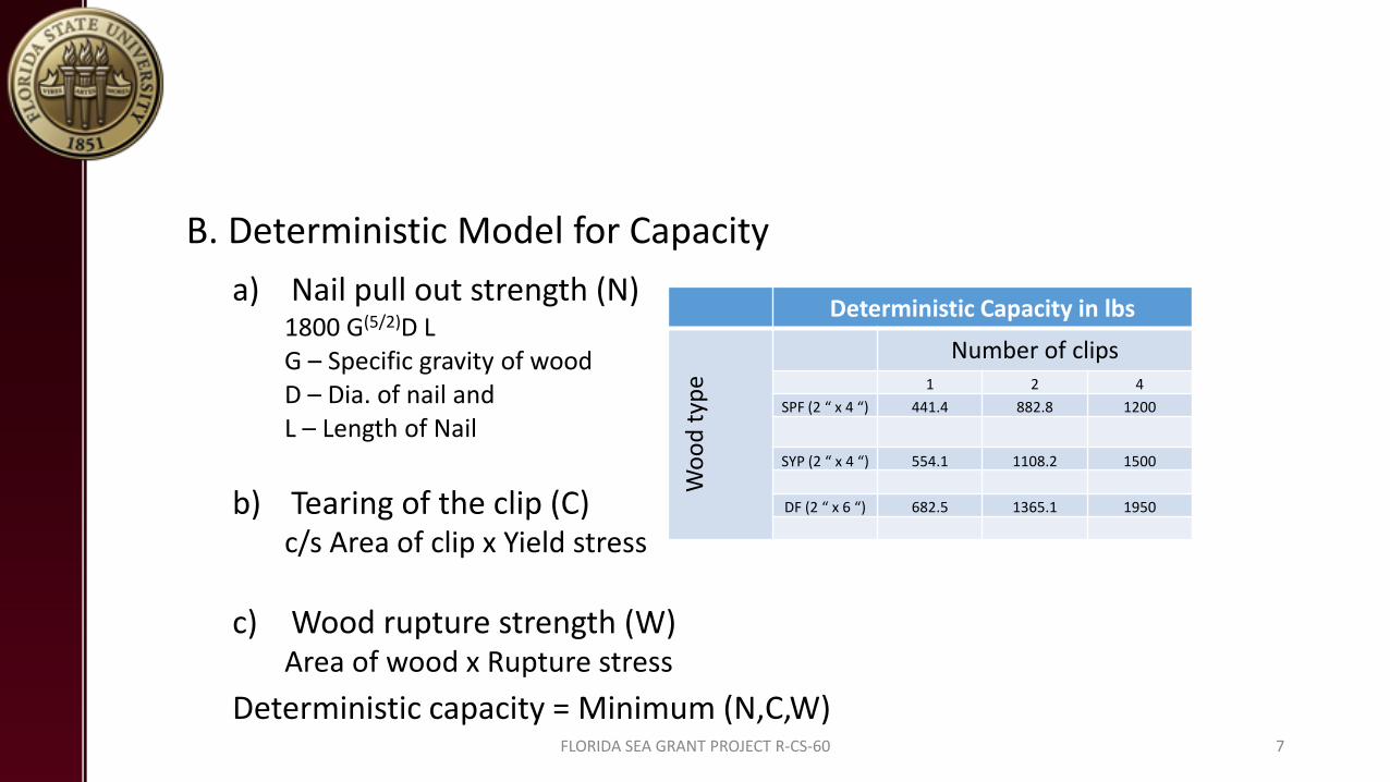
B.Deterministic

Model for Capacity

C.Capacity

Prediction Model

D.Fragility analysis

E.Comparison

of results

2. Tasks Completed

• 6 different sources - 1 PhD. Diss., 2 M. Thesis, 2 J. Publ., 1 T. Report

• Results of component level testing

• Categorized results based on number of clips and wood type Ex: Ahmed et al.(2011)

• Capacity depends on mode of failure which in turn depends on combination of number of clips and wood type.

FLORIDA SEA GRANT PROJECT R-CS-60 5

A. Compile Experimental Data

Ahmed et al. (2011) - H2.5A clips on (SPF,SYP and DF)

6

a) Nail pull out b) Clip tearing c) Wood splitting

A. Compile Experimental Data

Capacity in lbs – Mean and (Standard deviation)

Woo

d ty

pe

Number of clips1 2 4

SPF (2 “ x 4 “) 436.6 591.4 887.4(51.9) (68.3) (70.5)

SYP (2 “ x 4 “) 459 711.4 931.2(29.6) (65.8) (85.3)

DF (2 “ x 6 “) 640.2 753.2(53.1) (65.5)

Observed Modes of failure

Woo

d ty

pe


SPF (2 “ x 4 “) Nail pull out Wood split Wood split

SYP (2 “ x 4 “) Nail pull out Wood split Wood split

DF (2 “ x 6 “)Clip

deformation Clip tearing

a) Nail pull out strength (N)1800 G(5/2)D L G – Specific gravity of woodD – Dia. of nail andL – Length of Nail

b) Tearing of the clip (C)c/s Area of clip x Yield stress

c) Wood rupture strength (W)Area of wood x Rupture stress

Deterministic capacity = Minimum (N,C,W)FLORIDA SEA GRANT PROJECT R-CS-60 7

B. Deterministic Model for Capacity

Deterministic Capacity in lbs

Woo

d ty

pe


SPF (2 “ x 4 “) 441.4 882.8 1200

SYP (2 “ x 4 “) 554.1 1108.2 1500

DF (2 “ x 6 “) 682.5 1365.1 1950

C. Capacity Prediction Model→ Conventional Capacity Model

• The capacity follows a log-normal distribution

𝐶𝐶𝑐𝑐 = 𝐿𝐿𝐿𝐿(µ,σ)

• 𝐶𝐶𝑐𝑐 Conventional capacity value

• µ Mean value of capacity from experiments

• σ Standard deviation of capacity from experiments


C. Capacity Prediction Model→ Capacity Update Model

• The polynomial model for bias correction is as follows

𝐶𝐶𝑢𝑢 𝑥𝑥 = 𝜌𝜌 𝑥𝑥 𝐶𝐶𝑝𝑝 𝑥𝑥 + 𝛿𝛿 𝑥𝑥 + ε

• 𝐶𝐶𝑢𝑢 Updated capacity value

• 𝜌𝜌 Scale correction function

• 𝐶𝐶𝑝𝑝 Deterministic capacity

• 𝛿𝛿 Bias correction function (𝛿𝛿0+𝛿𝛿1 𝑥𝑥1+𝛿𝛿11 𝑥𝑥12+𝛿𝛿2 𝑥𝑥2+𝛿𝛿3 𝑥𝑥3)

• 𝑥𝑥1 Number of clips

• 𝑥𝑥2 , 𝑥𝑥3 Indicator variables for wood type.

• ε Random model error9FLORIDA SEA GRANT PROJECT R-CS-60

Statistical pooled model based on number of connection and wood type:

𝐶𝐶𝑒𝑒 𝑥𝑥 = 𝛿𝛿 𝑥𝑥 + ε

𝛿𝛿 Bias correction function (𝛿𝛿0+𝛿𝛿1 𝑥𝑥1+𝛿𝛿11 𝑥𝑥12+𝛿𝛿2 𝑥𝑥2+𝛿𝛿3 𝑥𝑥3)

𝑥𝑥1 Number of clips𝑥𝑥2 , 𝑥𝑥3 Indicator variables for wood type.ε Random model error


C. Capacity prediction model→ Statistical Pooled Model

Example • Residential building – Wood, Gable

roof (Cope, 2004)• Rigid, Fully enclosed, Exposure B• Length 56’, Breadth 44’, Wall height

10’, Roof slope 5:12 (θ =22.6°)• Eave overhang 2’, Truss spacing 2’• 1 and 2, H2.5A clips at each

connection.• SPF 2” x 4”

56’

44’

10’

9.2’

44’

Truss

Top plate

Column 11FLORIDA SEA GRANT PROJECT R-CS-60

D. Fragility Analysis


Example • Wind parallel to ridge• Region 3 and 4• Cpi = 0.18, Cp = -0.9, Cpov = 0.8• Force per connection=0.00256 x kz x kzt x kd x V2

x ( (Cp- Cpi)x(44/2)x2 + Cpov x 2 x 2 )

D. Fragility Analysis3

4


D. Fragility Analysis→ Conventional

• SPF, 1 H2.5A clip• Mean capacity = 436.6 lb• Std. deviation = 51.89 lb

• SPF, 2 H2.5A clip• Mean capacity = 591.4 lb• Std. deviation = 68.34 lb

Φ=

ζµ)/ln()( DvF𝐶𝐶𝑐𝑐 = 𝐿𝐿𝐿𝐿(µ,σ)

Log transformation• Quantile Quantile-plot of

regression model residuals and lognormal distribution

• Lognormal distribution is an adequate fit for model random errors

• Use logarithmic capacity values in the model


D. Fragility Analysis

-2.5 -2 -1.5 -1 -0.5 0 0.5 1 1.5 2 2.5-3

-2

-1

0

1

2

3

Quantiles of normal DistributionQ

uant

iles

of In

put S

ampl

e

QQ Plot of Sample Data versus Distribution

𝑃𝑃 𝐶𝐶𝑢𝑢 𝑋𝑋, 𝑥𝑥 = 𝑡𝑡𝜈𝜈 �𝑏𝑏′𝑥𝑥, 𝑠𝑠2(1 + 𝑥𝑥𝑥 𝑋𝑋𝑥𝑋𝑋 −1𝑥𝑥)

𝑥𝑥 Regressor vector 𝐶𝐶𝑝𝑝 1 𝑥𝑥1 𝑥𝑥2 𝑥𝑥12

𝐶𝐶𝑝𝑝 Computer prediction of capacity �𝑏𝑏 Coefficient vector 𝑋𝑋𝑥𝑋𝑋 −1𝑋𝑋′𝑦𝑦

𝑠𝑠2 Error variance 𝐿𝐿 − 𝑑𝑑 −1 𝐶𝐶𝑒𝑒 − 𝑋𝑋�𝑏𝑏′𝐶𝐶𝑒𝑒 − 𝑋𝑋�𝑏𝑏

𝜈𝜈 𝐿𝐿 − 𝑑𝑑𝐶𝐶𝑒𝑒 Vector of capacity observations

𝑋𝑋 Matrix of regressor observations 15

D. Fragility Analysis→ Proposed

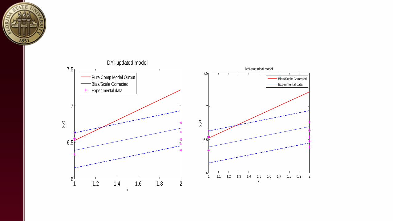
Posterior predictive distribution of updated capacity model


Updated capacity distribution• For a given number of clips

the predictive distribution of the capacity is a lognormal distribution.

• We calculate the probability of failure from these distributions.


17


Updated Model and Statistical Pooled Model

Assume 𝐷𝐷 is the wind-load effect, then the limit state due to wind failure is given

𝑔𝑔 𝛽𝛽, 𝑣𝑣 = 𝐶𝐶𝑢𝑢 𝑥𝑥,𝛽𝛽 − 𝐷𝐷(𝑣𝑣) ≤ 0The probability of failure at a given wind speed 𝑣𝑣 is found by integrating the predictive distribution:

𝑃𝑃𝑓𝑓𝑓𝑓 = 𝑃𝑃 𝑔𝑔 𝛽𝛽, 𝑣𝑣 ≤ 0 = �−∞

𝐷𝐷

𝑃𝑃 𝐶𝐶𝑢𝑢 𝑋𝑋, 𝑥𝑥



Failure Probability



Results

Proposed approach Conventional approach


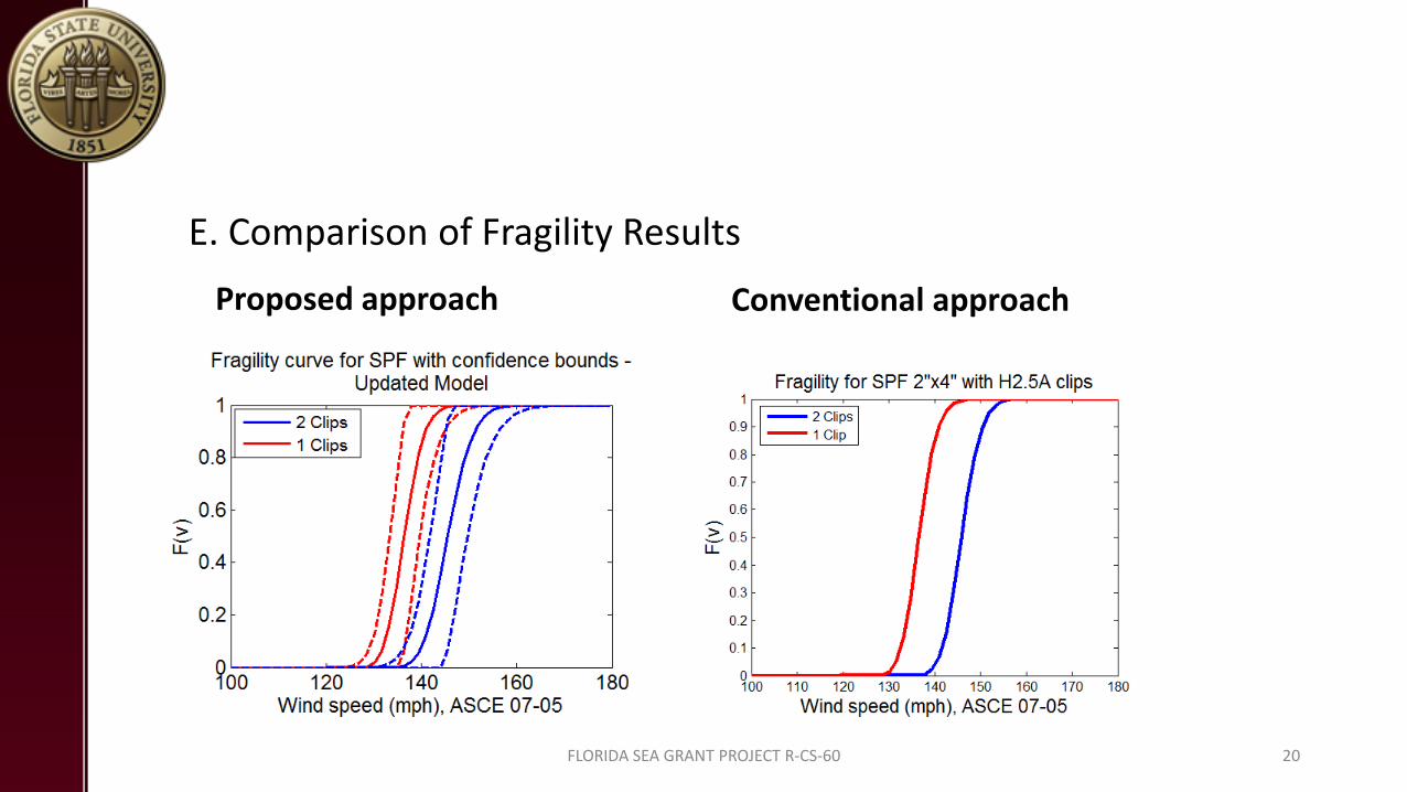
E. Comparison of Fragility Results

Bounds on wind speed at 0.50 failure probability • Bayesian approach allows us to

quantify the confidence in predictions of updated and statistical model.

• Computer updated model is not markedly improved than the statistical model for prediction uncertainty.


E. Comparison of fragility results

3. Summary

Bayesian based approaches in capacity prediction were studied

Fragility curves were obtained using predicted capacities.

Fragility curves from different approaches were compared


4. Future tasks

Demand uncertainty

Improve the deterministic capacity model

Improve the Bayesian model fit.

Improve bound estimation

Extreme value prediction

What EQECAT wants us to do ?23FLORIDA SEA GRANT PROJECT R-CS-60

Questions and Comments

?


References• S.S., Ahmed, I., Canino, A.G., Chowdhury, A., Mirmiran, N., Suksawang. (2011). “Study of the Capability of Multiple

Mechanical Fasteners in Roof-to-Wall Connections of Timber Residential Buildings.” Practice Periodical on Structural Design and Construction, 16, 2-9.

• K. G., Tyner, (1996).”Uplift capacity of rafter-to-wall connections in light-frame construction,” MS thesis, Dept. of Civil Engineering, Clemson University, Clemson, S.C.

• T.D., Reed (1997). “Wind resistance of roof systems in light-frame construction.” MS thesis, Dept. of Civil Engineering, Clemson University, Clemson, S.C.

• B., Shanmugam, (2011). “Probabilistic assessment of roof uplift capacities in low-rise residential construction” Doctoral dissertation, Dept. of Civil Engineering, Clemson University, Clemson, S.C.

• L.R., Canfield, S.H. Niu, H. Liu (1991). “Uplift resistance of various rafter-wall connections.” Forest Products Journal, 41, 27-34.

• J. Cheng (2004). “Testing and analysis of the toe-nail connection in the residential roof-to-wall system.” Forest Products Journal, 54, 58-65.

• P. Gardoni, A.D., Kiureghian, K. M. Mosalam (2002). “Probabilistic capacity models and fragility estimates for reinforced concrete columns based on experimental observations.” Journal of Engineering Mechanics, 128, 1024-1038.

• M. A. Riley, F., Sadek (2003). “Experimental testing roof to wall connections in wood frame houses.” Building and Fire Research Laboratory, National Institute of Standards and Technology, Gaithersburg, MD, USA.


Back up slides


Wind load estimation (Ch 27, ASCE - 07)

• V – Basic wind speed• Kz = 0.61 (velocity pressure

exposure coefficient)• Kzt = 1 (topographic constant)• Kd = 0.85 (Wind directionality

factor)


Wind load estimation – Parallel to ridge

• q = qi = 0.00256*Kz*Kzt*Kd*V2

• Self weight = 17 psf.• Cpi = +0.18,-0.18 (Internal pressure

coefficient) Figure 26.11-1• Cp (External pressure coefficient)

Figure 27.4-1.• Design wind pressure = qGCp - qiGCpi• Force on the sheathing = Area *(

Wind pressure – self wt. )• Fconnection =.00256 x kz x kzt x kd x V2 x

( (Cp- Cpi)x(44/2)x2 + Cpoverhang x 2 x2 )

34

56


1 1.5 2 2.5 3 3.5 4

6

6.2

6.4

6.6

6.8

7

7.2

7.4

x, Number of Connections

y(x

), C

ap

acity

SPF - updated model

Pure Model OutputExperimental dataPred of Updated95% PI of updated

1 1.5 2 2.5 3 3.5 4

6

6.2

6.4

6.6

6.8

7

7.2

7.4

x, Number of Connections

y(x)

, Ca

pa

city

SPF - statistical pooled model

Pure Comp ModelExperimental dataPred of Statistical95% PI of statistical

1 1.5 2 2.5 3 3.5 4

6

6.2

6.4

6.6

6.8

7

7.2

7.4

x

y(x)

SPY-updated model

Pure Comp Model OutputBias/Scale CorrectedExperimental data

1 1.5 2 2.5 3 3.5 4

6

6.2

6.4

6.6

6.8

7

7.2

7.4

x

y(x)

SPY - statistical model

Pure Comp ModelExperimental data95% PI of statistical

1 1.2 1.4 1.6 1.8 26

6.5

7

7.5

x

y(x

)DYI-updated model

Pure Comp Model OutputBias/Scale CorrectedExperimental data

1 1.1 1.2 1.3 1.4 1.5 1.6 1.7 1.8 1.9 26

6.5

7

7.5

x

y(x

)

DYI-statistical model

Bias/Scale CorrectedExperimental data

60 80 100 120 140 160 1800

0.2

0.4

0.6

0.8

1

wind speed (mph)

F(v

)

Fragility curve for SPF with confidence bounds- Updated Model

2 connection1 connection

60 80 100 120 140 160 1800

0.2

0.4

0.6

0.8

1

wind speed (mph)

F(v

)

Fragility curve for SPF with confidence bounds - Pooled Stat Mode


60 80 100 120 140 160 1800

0.2

0.4

0.6

0.8

1

wind speed (mph)

F(v

)Fragility curve for SPY with confidence bounds- Updated Model


60 80 100 120 140 160 1800

0.2

0.4

0.6

0.8

1

wind speed (mph)

F(v

)

Fragility curve for SPY with confidence bounds - Pooled Stat Mode


60 80 100 120 140 160 1800

0.2

0.4

0.6

0.8

1

wind speed (mph)

F(v

)Fragility curve for DYI with confidence bounds- Updated Model


60 80 100 120 140 160 1800

0.2

0.4

0.6

0.8

1

wind speed (mph)

F(v

)

Fragility curve for DYI with confidence bounds - Pooled Stat Mode


SPF

0.5 1 1.5 2 2.5130

140

150

160

170

180

model

win

d sp

eed,

mph

wind speed for 50% failure prob. 1: updated, 2: stat,

1 connect 2 connect 4 connect

SPY

0.5 1 1.5 2 2.5130

140

150

160

170

180

model

win

d sp

eed,

mph


1 connect 2 connect 4 connect

DYI

0.5 1 1.5 2 2.5140

145

150

155

160

165

model

win

d sp

eed,

mph


1 connect 2 connect

Date post:	11-Aug-2015
Category:	Documents
Upload:	bejoy-p-alduse-eit
View:	173 times
Download:	1 times

Promoting preventive mitigation of buildings against hurricanes

Documents