PROPAGATION OF ONE AND TWO-DIMENSIONAL DISCRETE WAVES UNDER FINITE DIFFERENCE APPROXIMATION UMBERTO BICCARI 1,2 , AURORA MARICA 3 , AND ENRIQUE ZUAZUA 1,2,4,5 Abstract. We analyze the propagation properties of the numerical versions of one and two-dimensional wave equations, semi-discretized in space by finite difference schemes. We focus on high-frequency solutions whose propagation can be described, both at the continuous and semi-discrete level, by micro-local tools. We do it both for uniform and non-uniform numerical grids and also for constant coefficients and variable ones. The energy of continuous and semi-discrete high-frequency solutions propagates along bi-characteristic rays, but their dynamics differ from the continuous to the semi-discrete setting, because of the different nature of the corresponding Hamiltonians. One of the main objectives of this paper is to illustrate through accurate numerical simulations that, in agreement with the micro-local theory, numerical high-frequency solutions can bend in an unexpected manner, as a result of the accumulation of the local effects introduced by the heterogeneity of the numerical grid. These effects are enhanced in the multi-dimensional case where the interaction and combination of such behaviors in the various space directions may produce, for instance, the rodeo effect, i. e. waves that are trapped by the numerical grid in closed loops, without ever getting to the exterior boundary. Our analysis allows explaining all such pathological behaviors. Moreover, the discussion in this paper also contributes to the existing theory about the necessity of filtering high-frequency numerical components when dealing with control and inversion problems for waves, which is based very much in the theory of rays and, in particular, on the fact that they can be observed when reaching the exterior boundary of the domain, a key property that can be lost through numerical discretization. 1. Introduction The analysis of propagation properties of numerical waves obtained through a finite difference discretization on uniform or non-uniform meshes is a topic which has been extensively investigated in the literature. Among other contributions, we mention the works [36, 37, 38, 39, 40, 41, 42]. In this paper, we are interested in discussing several aspects of wave propagation in a computational framework, and in the comparison with the usual behavior of the continuous models. In more detail, we consider here wave-like equations and their numerical approximation by a finite difference scheme, with the intent to illustrate theoretically and computationally the dynamics that this discretization introduces, and to comment the main differences with respect to the expected comportment of the original continuous PDE. Our analysis will address both constant and variable coefficients models, in one and two space dimensions. Moreover, our approach is based on the study of the propagation of high-frequency Gaussian beam solutions (that is, solutions originated from highly concentrated and oscillating initial data), both in continuous and discrete media. In a continuous setting, these kind of techniques date back to the works of H¨ormander ([21]), and they have been later extended by several authors, with the developments of tools like micro-local defect measures (introduced independently by G´ erard in [16] and by Tartar in [35], in the context of nonlinear partial differential equations and of homogenization, respectively) or Wigner measures ([24, 29, 44]) 2010 Mathematics Subject Classification. 35A21, 37C05, 65M06, 70K05. Key words and phrases. Wave equation, Finite difference approximation, Uniform and non-uniform meshes, Propagation of solutions. This project has received funding from the European Research Council (ERC) under the European Union’s Horizon 2020 research and innovation programme (grant agreement No. 694126-DyCon). The work of the first and of the third author was partially supported by the Grants MTM2014-52347 and MTM2017-92996 of MINECO (Spain) and by the Grant FA9550-18-1-0242 of AFOSR. The work of the second author was partially supported by CNCS-UEFISCDI Grant No. PN-III-P4-ID-PCE-2016-0035. The work of the third author was partially supported by the Grant ICON of the French ANR.. 1 arXiv:1806.09313v1 [math.AP] 25 Jun 2018
Transcript
PROPAGATION OF ONE AND TWO-DIMENSIONAL DISCRETE WAVES UNDER
FINITE DIFFERENCE APPROXIMATION
UMBERTO BICCARI1,2, AURORA MARICA3 , AND ENRIQUE ZUAZUA1,2,4,5
Abstract. We analyze the propagation properties of the numerical versions of one and two-dimensionalwave equations, semi-discretized in space by finite difference schemes. We focus on high-frequency solutions
whose propagation can be described, both at the continuous and semi-discrete level, by micro-local tools. Wedo it both for uniform and non-uniform numerical grids and also for constant coefficients and variable ones.The energy of continuous and semi-discrete high-frequency solutions propagates along bi-characteristic rays,but their dynamics differ from the continuous to the semi-discrete setting, because of the different nature of
the corresponding Hamiltonians. One of the main objectives of this paper is to illustrate through accuratenumerical simulations that, in agreement with the micro-local theory, numerical high-frequency solutionscan bend in an unexpected manner, as a result of the accumulation of the local effects introduced by the
heterogeneity of the numerical grid. These effects are enhanced in the multi-dimensional case where theinteraction and combination of such behaviors in the various space directions may produce, for instance, therodeo effect, i. e. waves that are trapped by the numerical grid in closed loops, without ever getting to theexterior boundary. Our analysis allows explaining all such pathological behaviors. Moreover, the discussion
in this paper also contributes to the existing theory about the necessity of filtering high-frequency numericalcomponents when dealing with control and inversion problems for waves, which is based very much in thetheory of rays and, in particular, on the fact that they can be observed when reaching the exterior boundaryof the domain, a key property that can be lost through numerical discretization.
1. Introduction
The analysis of propagation properties of numerical waves obtained through a finite difference discretizationon uniform or non-uniform meshes is a topic which has been extensively investigated in the literature. Amongother contributions, we mention the works [36, 37, 38, 39, 40, 41, 42].
In this paper, we are interested in discussing several aspects of wave propagation in a computationalframework, and in the comparison with the usual behavior of the continuous models. In more detail, weconsider here wave-like equations and their numerical approximation by a finite difference scheme, with theintent to illustrate theoretically and computationally the dynamics that this discretization introduces, and tocomment the main differences with respect to the expected comportment of the original continuous PDE.
Our analysis will address both constant and variable coefficients models, in one and two space dimensions.Moreover, our approach is based on the study of the propagation of high-frequency Gaussian beam solutions(that is, solutions originated from highly concentrated and oscillating initial data), both in continuous anddiscrete media.
In a continuous setting, these kind of techniques date back to the works of Hormander ([21]), and theyhave been later extended by several authors, with the developments of tools like micro-local defect measures(introduced independently by Gerard in [16] and by Tartar in [35], in the context of nonlinear partialdifferential equations and of homogenization, respectively) or Wigner measures ([24, 29, 44])
2010 Mathematics Subject Classification. 35A21, 37C05, 65M06, 70K05.Key words and phrases. Wave equation, Finite difference approximation, Uniform and non-uniform meshes, Propagation of
solutions.This project has received funding from the European Research Council (ERC) under the European Union’s Horizon 2020
research and innovation programme (grant agreement No. 694126-DyCon). The work of the first and of the third author was
partially supported by the Grants MTM2014-52347 and MTM2017-92996 of MINECO (Spain) and by the Grant FA9550-18-1-0242of AFOSR. The work of the second author was partially supported by CNCS-UEFISCDI Grant No. PN-III-P4-ID-PCE-2016-0035.The work of the third author was partially supported by the Grant ICON of the French ANR..
1
arX
iv:1
806.
0931
3v1
[m
ath.
AP]
25
Jun
2018
More recently, this same question has been addressed also at the numerical level, and we can nowadaysmention contributions on the extension of micro-local techniques to the study of the propagation propertiesfor discrete waves ([26, 28]).
Roughly speaking, the idea at the basis of this techniques is that the energy of Gaussian beam solutionspropagates along bi-characteristic rays, which are obtained from the Hamiltonian system associated to thesymbol of the operator under consideration. At the continuous level, if the coefficients of the equation areconstants, these mentioned rays are straight lines and travel with a uniform velocity. In the case of variablecoefficients, instead, the heterogeneity of the medium where waves propagate produces the bending of therays and, consequently, the increasing or the decreasing of their velocity.
On the other hand, the finite difference space semi-discretization of the equation may introduce differentdynamics, with a series of unexpected propagation properties at high frequencies, that substantially differ fromthe expected behavior of the continuous equation. For instance, one can generate spurious solutions travelingat arbitrarily small velocities ([37]) which, therefore, show lack of propagation in space. As we shall see, thisphenomenon is related with the particular nature of the discrete group velocity which, differently from thecontinuous equation, may vanish at certain frequencies. In addition, the introduction of a non-uniform meshfor the discretization of the equation makes the situation even more intricate. For instance, as indicated in[28, 41], for some numerical grids the rays of geometric optics may present internal reflections, meaning thatthe waves change direction without hitting the boundary.
All these pathologies are purely numerical, and they are related to changes in the Hamiltonian systemgiving the equations of the rays. Actually, as we will discuss with more details later, they can be rigorouslyexplained by the behavior of the corresponding phase portrait.
With this considerations in mind, our main goal in the present article is to exhibit the kind of spuriouseffects one may encounter when performing numerical approximations by means of finite difference schemes.Our principal contribution is the detection of these singular phenomena in the numerical propagation of thewaves.
More than on the presentation of the mathematical details, in this article we focus on a self containedreview of the propagation properties of the numerical solutions of discrete wave equations, with the support ofseveral numerical simulations showing the aforementioned pathologies. For a more complete and exhaustivediscussion on this topic, the interested reader may refer also to [26, 27, 28]. We start by considering thefollowing one-dimensional system
∂2t u− ∂2
xu = 0, (x, t) ∈ (−1, 1)× (0, T )
u(−1, t) = u(1, t) = 0, t ∈ (0, T )
u(x, 0) = u0(x), ∂tu(x, 0) = u1(x), x ∈ (−1, 1),
(1.1)
A classical property of the above equation is that its total energy, is conserved in time. In other words, ifwe define the energy associated to (1.1) as the quantity
E(u, ∂tu) :=1
2
∫ 1
−1
(|∂tu|2 + |∂xu|2
)dx, (1.2)
we then have
E(u, ∂tu) = E(u0, u1), ∀ t ∈ (0, T ).
Moreover, when x ∈ R, according to the d’Alembert formula
u(x, t) =1
2
(u0(x+ t) + u0(x− t)
)+
1
2
∫ x+t
x−tu1(z) dz (1.3)
the solution can be uniquely decomposed into two waves, each one of them propagating along one of thestraight characteristics x ± t. In addition, it is well-known (see [3, 6, 7, 26, 27, 33, 34]) that the energyof initial data presenting high-frequency oscillation and/or concentration effects propagates along thesecharacteristic rays.
As we mentioned, these concentration features can be observed also at the numerical level but, in thisframework, the high-frequency solutions exhibit several pathological behaviors. In order to detect and describe
2
these propagation properties, we are going to discretize (1.1) through a finite difference scheme for the spacevariable and a classical leapfrog method for the time integration.
Moreover, the analysis that we are going to present can be easily extended also to the case of variablecoefficients and to multi-dimensional problems. In fact, in the second part of this paper we will briefly discussthe following one-dimensional variable coefficients wave equation
ρ(x)∂2t u− ∂x
(σ(x)∂xu
)= 0, (x, t) ∈ (−1, 1)× (0, T )
u(−1, t) = u(1, t) = 0, t ∈ (0, T )
u(x, 0) = u0(x), ∂tu(x, 0) = u1(x), x ∈ (−1, 1),
(1.4)
where ρ and σ are chosen to be L∞(R)-functions with the strict hyperbolicity assumption ρ(x) ≥ ρ∗ > 0 andσ(x) ≥ σ∗ > 0.
Even if for (1.4) there is no explicit formula for the solutions analogous to (1.3), it still holds that highlyconcentrated and oscillatory initial data lead to Gaussian wave packet-type solutions concentrated alongone of the bi-characteristics (which are not straight lines anymore), and their energy localized outside anyneighborhood of the ray vanishes as the wavelength parameter tends to zero.
Once again, these concentration features can be observed also at the numerical level. Moreover, also inthis case the space semi-discretization of (1.4) may introduce dynamics different than the ones that we wouldexpect from the analysis of the continuous equation. We will present some of these phenomena later in themanuscript.
Lastly, the final part of the present work will be devoted to a brief discussion of the following two-dimensional system
ρ(z)∂2t u− divz
(σ(z)∇zu
)= 0, (z, t) ∈ Ω× (0,+∞)
u|∂Ω = 0, t ∈ (0,+∞)
u(z, 0) = u0(z), ∂tu(z, 0) = u1(z), z ∈ Ω,
(1.5)
where we indicate Ω := (−1, 1)2 and in which the same assumptions on the coefficients ρ and σ will beconsidered.
For the sake of completeness, let us conclude this introduction by mentioning that our study is motivatedby control and inverse problems. Indeed, it is well-known that boundary controllability and identifiabilityproperties of solutions of wave equations hold because of the fact that the energy is driven by characteristicsthat reach a subregion of the domain or of its boundary where the controllers or observers are placed. This,in particular, allows the observability of the solutions (namely, the possibility to obtain estimates of the totalenergy in terms of the energy concentrated on the support of the control along time), which is classicallyknown to be equivalent to control properties.
In the framework of wave-like processes, observability is guaranteed by the so-called geometric controlcondition (GCC), requiring all rays of geometric optics to enter the control region during the control time.This condition has been proved to be sufficient and almost necessary in [3] (see also [6, 7]). In particular, thenecessity of GCC is related to the fact that, around each ray that does not meet the observation/controlregion, one can always build concentrated Gaussian beams making the observability inequality impossible.
When the wave equation is approximated by finite difference methods on uniform meshes, the controlfor the discretized model does not necessarily yields a good approximation of the control for the originalcontinuous problem. Instead, observability/controllability may be lost under numerical discretization asthe mesh size tends to zero, due to the existence of high-frequency spurious solutions for which the groupvelocity vanishes. In particular, it is by now well-known that the discretization of the equation generateswave packets traveling with a group velocity which, at high frequencies, is of the order of 1/h, h being thespace mesh size. These high-frequency solutions are such that the energy concentrated in the control region isasymptotically smaller than the total energy, and they produce the exponential blow-up of the observabilityconstant as h→ 0. A deeper discussion on this topic is out of the scope of the present paper and, therefore, itwill not be considered here. The interested reader may refer to the well extended bibliography on the controlproperties for discrete waves [8, 13, 14, 15, 17, 18, 20, 22, 23, 25, 26, 27, 30, 31, 45, 46]).
This paper is organized as follows. In Section 2, we discuss the one-dimensional case. In more detail, inSection 2.1 we are going to introduce the finite difference discretization of the one-dimensional model (1.1). In
3
Section 2.2, we will present and discuss the Hamiltonian system, giving the equations for the bi-characteristicrays, while Section 2.3 will be devoted to show and comment the results of our numerical simulations. We willcomplete this first part of the paper with Section 2.5, which is devoted to the case of a variable-coefficientswave equation. Finally, in Section 3, we will briefly consider the extension of our analysis to two-dimensionalproblems.
2. One-dimensional wave equation
We discuss here the propagation properties of the finite difference approximation of the solution to theone-dimensional wave equation (1.1). We start by introducing the numerical scheme that we will employ.
2.1. Semi-discrete approximation of (1.1). Let us introduce the grid and the space semi-discrete ap-proximation of (1.1) that we will employ in our analysis.
Let g : [−1, 1]→ [−1, 1] be a diffeomorphism. For N ∈ N∗, we set h = 2/(N + 1) as the step size of theuniform mesh
Gh :=xj := −1 + jh, j = 0, . . . , N + 1
,
and we consider the non-uniform grid
Ghg :=gj := g(xj), xj ∈ Gh
obtained by transforming Gh through the map g.
• •• • • • • • • • •• • • • • • •xj gj
g
uniform mesh non-uniform mesh
−1 −11 1
Figure 1. The diffeomorphism g transform the nodes xj of the uniform mesh Gh into thenodes gj of the non-uniform one Ghg .
Along all this paper, we focus on the case in which g is regular. More precisely, we assume that g ∈ C2(R)with 0 < g−d ≤ |g′(x)| ≤ g+
d < +∞ and |g′′(x)| ≤ gdd < +∞ for some given constant g−d , g+d , gdd > 0 and for
all x ∈ R. We stress that this also includes the case of a uniform grid, that is g(x) = x.Notice that the above assumptions yield that 1/g′ belongs to the space C0,1(R) of the Lipschitz continuous
functions. As we will see in the next section, this Lipschitz regularity assumption will be important whenintroducing the Hamiltonian system for the bi-characteristic rays.
We set gj+1/2 := g(xj+1/2) to be the image through the map g of the midpoints xj+1/2 := −1 + (j + 1/2)h,and we denote by
hj+1/2 := gj+1 − gj , j = 0, . . . , N
hj−1/2 := gj − gj−1, j = 1, . . . , N + 1
hj :=hj+1/2 − hj−1/2
2, j = 1, . . . , N
the heterogeneous mesh sizes. The semi-discretization of the wave equation (2.13) on the non-uniform gridGhg is then given as follows:
hju′′j (t)−
(uj+1(t)− uj(t)
hj+1/2− uj(t)− uj−1(t)
hj−1/2
)= 0, j = 1, . . . , N, t ∈ (0, T )
u0(t) = uN+1(t) = 0, t ∈ (0, T )
uj(0) = u0j , u′j(0) = u1
j , j = 1, . . . , N.
(2.1)
4
Here we indicate uj(t) := u(gj , t). Moreover, to avoid possible confusions, when needed, we will denote
the solutions of (2.17) by uh,g(t) := (ugj (t))N+1j=0 for emphasizing the dependence from the diffeomorphic
transformation g. But, in general, we will simply write down uh(t) := (uj(t))N+1j=0 , u0,h := (u0
j)N+1j=0 and
u1,h := (u1j )N+1j=0 for the solutions and for the initial data.
It has been shown in [28, Proposition 3.4] that, under our regularity assumptions on the mesh function g,the numerical approximation (2.1) with initial data (u0,h,u1,h) is a convergent scheme of order O(h) for thewave equation (1.1) in the appropriate `2 setting. Moreover, it can be readily checked that, as it happens forthe continuous model, system (2.1) enjoys the property of energy conservation, that is,
Eh,g(uh,g(t), ∂tuh,g(t)) :=1
2
N∑j=1
hj |∂tugj (t)|2 +
1
2
N∑j=1
hj+1/2
∣∣∣∣∣ugj+1(t)− ugj (t)hj+1/2
∣∣∣∣∣2
= Eh,g(u0,h,u1,h).
2.2. The Hamiltonian system. As we mentioned in the introduction, it is classically known (see [3])that at the basis of the analysis of the observability properties of the continuous wave equation in anyspace dimension there are the propagation properties of bi-characteristic rays, leading to the so-calledGeometric Control Condition (GCC). This same analysis can be repeated also at the numerical level, and theobservability of the discrete wave equation (2.1) can be discussed through the study of the propagation ofdiscrete bi-characteristic rays.
Rays of geometric optics are defined as the projections on the physical space (x, t) of the bi-characteristicrays given by the Hamiltonian corresponding to the principal part of the operator. In the case of theone-dimensional wave equation (1.1), this Hamiltonian is given by
Hc(x, t, ξ, τ) = −τ2 + ξ2, (2.2)
and the bi-characteristic rays are the curves s 7→ (x(s), t(s), ξ(s), τ(s)) solving the first order ODE systemx(s) = ∂ξHc(x(s), t(s), ξ(s), τ(s)) = 2ξ(s)
t(s) = ∂τHc(x(s), t(s), ξ(s), τ(s)) = −2τ(s)
ξ(s) = −∂xHc(x(s), t(s), ξ(s), τ(s)) = 0
τ(s) = −∂tHc(x(s), t(s), ξ(s), τ(s)) = 0.
(2.3)
In (2.3), we indicate with x the time derivative of the variable x, for differentiating it from the notation′ that we are using for general derivatives. Moreover, to system (2.3) we associate an initial datum(x(0), t(0), ξ(0), τ(0)) = (x0, 0, ξ0, τ0) such that Hc(x0, 0, ξ0, τ0) = 0.
It is immediately seen that the above system can be explicitly solved, and we thus obtain that for any ξ0there are two characteristics starting from the point x0 which are given by the straight lines x±(t) = x0 ∓ t.Moreover, each one of these characteristics reaches the boundary of the interval (−1, 1) in a uniform timenot depending on the frequency ξ0. Then, when hitting the boundary, the ray reflects according to theDescartes-Snell’s law.
At the discrete level, the situation changes and it is more delicate. As a first thing, one needs to find asuitable counterpart of the Hamiltonian (2.2). This was done in [26] for the discrete wave equation in aninfinite lattice (i.e. with no boundary) and, more recently, the analysis was extended in [28] to non-uniformmeshes obtained by means of a C2 diffeomorphism.
To be more precise, in [28] the authors constructed solutions of (2.1) with frequencies of the order of1/h, localized around the rays of geometric optics given by the projection on the physical space of thebi-characteristic curves provided by the Hamiltonian
H(y, t, ξ, τ) = −g′(y)τ2 + 4 sin2
(ξ
2
)1
g′(y), y = g−1(x), (2.4)
or equivalently
H(y, t, ξ, τ) = −τ2 +1
g′(y)2ω(ξ)2, (2.5)
5
with
ω(ξ) := 2 sin
(ξ
2
).
We observe some changes in this discrete symbol with respect to the continuous one. Firstly, it dependson the space variable y = g−1(x) corresponding to the uniform grid. Note also the appearance of the factor1/g′(x) accompanying each space derivative, which is also due to the grid transformation. Moreover, theFourier symbol ξ2 of the second-order space derivative has been replaced by the corresponding symbol4 sin2(ξ/2) of the three-point finite difference approximation of the Laplacian. Lastly, observe that in thesymbol the parameter h disappears. This is due to the fact that we are analyzing the propagation of wavesof wavelength of the order of h.
Set cg := 1/g′. It is easy to see that from the discrete Hamiltonian (2.4) the ODE system for the rays thatone obtains is the following
y(s) = 2cg(y(s))2ω(ξ(s))∂ξω(ξ(s))
t(s) = −2τ(s)
ξ(s) = −2cg(y(s))∂ycg(y(s))ω(ξ(s))2
τ(s) = 0,
(2.6)
with an initial condition at s = 0 given by (y0, 0, ξ0, τ0) satisfying H(y0, 0, ξ0, τ0) = 0.In (2.6), ∂ξω(ξ) is the group velocity, i.e. the speed at which the energy associated with wave number ξ
moves. As it is natural to expect, this quantity has a fundamental role in the analysis of the propagation ofnumerical solutions.
To better understand the dynamics of the bi-characteristic rays remark that, for all s, τ(s) = τ0. Besides,H(y(s), t(s), ξ(s), τ(s)) = 0, so that for all s we encounter two different possible values for τ0, namely
τ±0 = ±cg(y(s))|ω(ξ(s))|.
Now, as dt/ds does not vanish, the Inverse Function Theorem allows to parametrize the curve s 7→(y(s), t(s), ξ(s), τ±0 ) by t 7→ (y(t), t, ξ(t), τ±0 ), hence obtaining
y±(t) = − 1
τ±0cg(y
±(t))2ω(ξ±(t))∂ξω(ξ±(t))
ξ±(t) =1
τ±0cg(y
±(t))∂ycg(y±(t))ω(ξ±(t))2
y±(0) = y0, ξ±(0) = ξ0,
(2.7)
or, equivalently, y±(t) = ∓cg(y±(t))∂ξω(ξ±(t))
ξ±(t) = ±∂ycg(y±(t))ω(ξ±(t))
y±(0) = y0, ξ±(0) = ξ0
(2.8)
Since by assumption cg(·) > 0, thanks to (2.8) we immediately see that
|y±(t)| = cg(y±(t))
∣∣∂ξω(ξ±(t))∣∣ .
In view of that, the velocity of the rays vanishes if, and only if, ∂ξ(ω) = 0 for some ξ. When ω(ξ) = ξ,corresponding to the continuous case, this cannot happen. Actually, in this case the rays travel with velocityone until they hit the boundary, where they are reflected. On the other hand, when ω(ξ) = 2 sin(ξ/2),corresponding to the finite difference discretization that we are considering, we immediately see that∂ξω(ξ) = cos(ξ/2) vanishes for ξ = (2k + 1)π, k ∈ Z. As our simulations will highlight, in this case we havethe phenomenon of non-propagating waves. Notice also that the possibility that the velocity of the discreterays is zero is independent of the choice of the mesh and of the variable coefficients. In other words, nomatter whether the coefficients are constant or variables, and no matter what mesh we select for solvingour problem, there will always be certain frequencies for which the group velocity of the numerical wavesvanishes.
6
2.3. Numerical results. We present several numerical simulations showing the propagation of the solutionsto (1.1) with highly concentrated and oscillating initial data.
Set xh to be the uniform mesh of size h = 2/(N + 1). We consider two non-uniform grids produced by thetransformations
g1 := tan(π
4x)
and g2(x) := 2 sin(π
6x), (2.9)
yielding a gradual refinement at the center x = 0 of the space interval and at the two endpoints x = ±1,respectively (see Figure 2). In what follows, we will indicate
gh,1 := g1(xh) = tan(π
4xh)
and gh,2 := g2(xh) = 2 sin(π
6xh).
Grid gh,1 Grid gh,2
Figure 2. Representation of the two non-uniform grids gh,1 and gh,2. By cross markerswe indicate the grid points and by solid line the application gi generating them.
The time discretization is done by means of a leap-frog scheme (un+1 − 2un + un−1)/(δt)2 with Courant-Fiedrichs-Lewy (CFL) condition δt = 0.1 · h (which is necessary since the method is explicit). Moreover, theinitial data are constructed starting from the following Gaussian profile
Gγ(x) = e−γ2
(g−1(x)−g−1(x0)
)2e i
ξ0h g−1(x), γ := h−0.9. (2.10)
In more detail, we will take u0,h = Gγ(gh,i), i = 1, 2, and u1,h = G′γ(gh,i). Moreover, in what follows wewill always assume ξ ∈ [0, 2π].
In our further discussion, it will be fundamental a deeper analysis of the Hamiltonian system associated to(2.1) which, we recall, is given by (see also (2.8))
y±(t) = ∓cg(y±(t)) cos
(ξ±(t)
2
)ξ±(t) = ±2∂ycg(y
±(t)) sin
(ξ±(t)
2
)y±(0) = y0, ξ±(0) = ξ0.
Recall also that in the above system the variable y = g−1(x) is the one corresponding to the refined mesh.In the original variable x = g(y) associated to the uniform partition of the space interval [−1, 1], (2.8) readsinstead as
x±(t) = ∓ag(x±(t)) cos
(ξ±(t)
2
)ξ±(t) = ±2bg(x
±(t)) sin
(ξ±(t)
2
)x±(0) = x0, ξ±(0) = ξ0.
7
with ag(·) := (g′cg)(g−1(·)), bg(·) := c′g(g
−1(·)) and, clearly, x0 = g(y0).Notice that, independently of the choice of the function g, we always have ag ≡ 1. Moreover, for each one
of the functions that we are considering for our mesh refinement also bg can be computed explicitly. In moredetail, we have
g(y) = tan(π
4y)
⇒ bg(x) = − 2x
x2 + 1
g(y) = 2 sin(π
6y)⇒ bg(x) =
x
4− x2,
and the Hamiltonian systems become
g(y) = tan(π
4y)⇒
x±(t) = ∓ cos
(ξ±(t)
2
)ξ±(t) = ∓ 4x±(t)
x±(t)2 + 1sin
(ξ±(t)
2
)x±(0) = x0, ξ±(0) = ξ0
(2.11)
and
g(y) = 2 sin(π
6y)⇒
x±(t) = ∓ cos
(ξ±(t)
2
)ξ±(t) = ± 2x±(t)
4− x±(t)2sin
(ξ±(t)
2
)x±(0) = x0, ξ±(0) = ξ0.
(2.12)
2.4. Discrete phase portraits and their interpretation. To help us in our further discussion, we includein Figure 3 the phase diagrams corresponding to (2.11) and (2.12), i.e. to the Hamiltonian system associatedto (2.1) on the two non-uniform meshes that we selected. The case of a uniform mesh is not displayed theresince, the related discrete symbol being independent of the variable x, the orbits would simply be straightlines parallel to the horizontal axis.
Figure 3. Phase portrait of the Hamiltonian system for the numerical wave equationand the grid transformations gh,1 (left) and gh,2 (right). We put x±(t), ξ±(t) on thehorizontal/vertical direction.
A couple of additional comments are needed here. First of all, in both phase diagrams we have a uniqueequilibrium in the point Pe := (xe, ξe) = (0, π) (the green one). Nevertheless, the nature of this equilibriumchanges when changing the mesh function. This is easily seen by considering the linearization of (2.11) and(2.12) around Pe, which is given by the linear systems(
x±
ξ±
)= Agi
(x±
ξ±
), i = 1, 2,
8
with
Ag1 :=
(0 1/2−4 0
)and Ag2 :=
(0 1/2
1/2 0
).
In the first case, it can be readily checked that the eigenvalues of Ag1 are λ1,2 = ±i√
2, i.e. they are purelyimaginary. In view of that, we can conclude that Pe is a center. On the other hand, for the other meshrefinement that we are considering, the eigenvalues of Ag2 are λ1,2 = ±1/2, that is, they are purely real withopposite signs. This implies that this times the fixed point is a saddle.
The second observation is related to the range of frequencies that we chose to include in our phase diagrams.In principle, the most suitable choice for the domain of the phase variable in this finite difference settingwould be ξ ∈ [−π, π] this being related essentially to the 2π-periodicity of the discrete Wigner transform andto the fact that the solutions of our semi-discrete wave equation may be written as linear combinations ofmonochromatic waves given by the complex exponentials
e±ij
(√λjjπ t−x
), j ∈ 1 . . . N,
λj := (4/h2) sin (jπh/2) being the eigenvalues of the one-dimensional finite difference Dirichlet Laplacian (see[26, 28, 46] and the references therein). In view of that, the relevant range of frequencies for the semi-discretewaves is ξ ∈ [0, π], and considering ξ ∈ [−π, π] in the phase portraits takes into account the two branches ofthe associated bi-characteristic rays.
Despite of these considerations, in Figure 3 we chose to take in to account a range of frequencies ξ ∈ [0, 2π],since we believe that in this way it is more visible the stable/unstable nature of the equilibrium points.Consequently, our phase diagrams have to be interpreted as showing in the upper part ξ ∈ [π, 2π] whatwould actually correspond to ξ ∈ [−π, 0]. To better understand this fact, let us follow, for instance, one ofthe blue orbits in the lower part of the portraits, corresponding to some given initial frequency ξ0 close tozero. The wave corresponding to this trajectory starts propagating to the left, until it hits the boundary ofthe physical domain (−1, 1) (indicated with the two black dotted lines) with a frequency ξ1 > ξ0. Then, itreflects according to the laws of geometric optics, and starts propagating to the right, along a trajectory inthe phase portrait whose initial frequency is ξ2 = 2π− ξ1. Notice that, if we were considering a phase portraiton [−π, π] instead of on [0, 2π], the initial frequency of the reflected trajectory would instead be ξ2 = −ξ1.
We now present and analyze the results of our simulations. In all this part, if not specified, we alwaysconsider a time horizon T = 5s. Moreover, since the solution to (2.1) starting from an initial datum as in(2.10) is complex, in our plots we decided to show its modulus.
We start by observing that, at low frequencies (that is, ξ ∈ [0, π] but not too close to ξ = π), the numericalsolutions of (2.1) behave basically like the solution of the continuous model (1.1): it starts traveling tothe left along the straight characteristic line x+ t and, after having hit the boundary, it reflects followingthe Descartes-Snell’s law and continues propagating, this time to the left along the other branch of thecharacteristic (x− t).
Figure 4. Propagation of a Gaussianwave packet for the finite differencescheme of equation (2.1) on the non-uniform mesh gh,1 at frequency ξ0 = π/4.We put on the horizontal axis the spacedomain (−1, 1) and on the vertical on thetime domain (0, T ).
Moreover, it can be seen in Figure 5 that an analogous but specular behavior is encountered also forfrequencies ξ ∈ [π, 2π] sufficiently close to ξ = 2π. This is in accordance with the discussion in the last partof Section 2.4.
9
Figure 5. Numerical solutions with x0 = 0, ξ0 = 7π/4 = 2π − π/4 and uniform mesh (left),non-uniform mesh gh,1 (middle) and non-uniform mesh gh,2 (right).
When increasing the frequency, instead, the situation changes and we encounter several interestingphenomena and pathologies:
• Non-propagating waves, corresponding to equilibrium (fixed) points on the phase diagram.• The so-called umklapp or U-process, also known as internal reflection (see [40]), consisting in the
reflection of waves without touching only one or both the endpoints of the space interval.
All these phenomena can be justified through the discussion that we introduced before and by looking atthe phase portrait of the rays.
2.4.1. Non-propagating waves. In Figure 6 we observe waves that do not propagate. As we can see from theplots, and as we were mentioning before, this happens both with uniform and non-uniform meshes.
Figure 6. Numerical solutions with x0 = 0, ξ0 = π and uniform mesh (left), non-uniformmesh gh,1 (middle) and non-uniform mesh gh,2 (right).
The justification to this fact is that, as we saw in the previous section, for ξ = π we have ∂ξω(ξ) = 0 and,therefore, the velocity of the rays vanishes.
However, we notice a big difference between the two plots corresponding to a non-uniform grid, concerningthe dispersion along the ray. When solving using the mesh gh,1, the wave remains concentrated along theray, while when using the mesh gh,2 the wave is very dispersive. This fact finds explanation in the analysisof the phase portrait associated to (2.11) and (2.12). In both cases the non propagating wave corresponds tothe only equilibrium point Pe := (xe, ξe) = (0, π) (the green one) on the corresponding phase diagrams inFigure 3. Nevertheless, as we observed in Section 2.4, the nature of this equilibrium changes when changingthe mesh function: for the grid gh,1, the point Pe is a center and, therefore, it produces a non-dispersivewave. On the other hand, for the other mesh refinement that we are considering, the fixed point is a saddleand, being this an unstable equilibrium, it generates the dispersion displayed in Figure 6.
2.4.2. Internal reflection. It is well known that, for the continuous case or for numerical waves on uniformmeshes concentrated on frequencies where the group velocity is not trivial, all the generalized rays are straightlines reflecting at both endpoints. Instead, when the mesh is non-uniform, we observe that certain solutions
10
to our wave equation do not preserve this behavior. In particular, our simulations show the following twopathologies:
(i) waves oscillating in the interior of the computational domain and reflecting without touching theboundary (see Figure 7);
(ii) waves that oscillate in the interior of the domain and reflect touching the boundary only at one ofthe endpoints (see Figure 8).
These trapped rays correspond to trajectories which remain always in the red area of the phase portraitsin Figure 3. More precisely, the situation (i) appears when employing the mesh gh,1, and it corresponds toperiodic orbits in the phase diagram which are completely included in the region between the two dottedblack vertical asymptotes indicating the computational domain [−1, 1].
Figure 7. Numerical solutions corresponding to the mesh gh,1 with x0 = 0 and ξ0 = 7π/15(left), ξ0 = 10π/15 (middle) and ξ0 = 13π/15 (right).
Notice that, as the frequency increases towards ξ = π, the amplitude of the oscillation decreases, the limitcase being the non-propagating wave of Figure 6.
Moreover, this phenomena can be explained if we consider that the mesh gh,1 is an expanding one, meaningthat the step size increases approaching the endpoints of the domain. Consequently, the group velocity 1/hof the high-frequency waves decreases while moving away from x = 0. If this group velocity vanishes beforethe wave has reached the boundary, then this results in a process of internal reflection.
Furthermore, the non-uniformity of the mesh size h is also responsible of the increasing and decreasing ofthe magnitude of the solution during its propagation (roughly speaking, the change of color from yellow tored in our plots). Indeed, the amplitude of the wave is the one of the Gaussian profile of the initial datum,which is given by the constant γ in (2.10) and depends on h. In particular, on the mesh gh,1 that we areusing in Figure 7, while approaching the boundary h increases. Therefore, the support of the ray shrinks and,due to energy conservation, the high of the corresponding wave has to increase since the same amount ofenergy is now concentrated in a smaller region. Then, when moving again towards the center of the physicaldomain, where h is smaller, the support of the ray increases again and the magnitude of the wave decreases.
Let us now conclude by briefly discussing the situation (ii), which appears when employing the mesh gh,2.Recall that in this case Pe is a saddle point, which is characterized by the fact that the space around it isdivided into four sectors by two curves (the separatrices) passing through the equilibrium. In view of that,the red curves always remain trapped either in the region x ∈ [0, 1] (Figure 8a) or x ∈ [−1, 0] (Figure 8b).Moreover, notice that this time the mesh is coarser around x = 0. On the one hand, this this implies thatthe velocity of high-frequency waves may vanish approaching the center of the domain, thus generatingagain some internal reflection phenomena. On the other hand, this reflects again on the increasing of themagnitude of the wave, according to the discussion that we presented above.
2.5. The case of variable coefficients. We discuss briefly here the case of the variable coefficients waveequation. In more detail, the model that we are going to consider is the following
ρ(x)∂2t u− ∂x
(σ(x)∂xu
)= 0, (x, t) ∈ (−1, 1)× (0, T )
u(−1, t) = u(1, t) = 0, t ∈ (0, T )
u(x, 0) = u0(x), ∂tu(x, 0) = u1(x), x ∈ (−1, 1),
(2.13)
11
(a) x0 = 1/2 (b) x0 = −1/2
Figure 8. Numerical solutions corresponding to the mesh gh,2 with x0 = ±1/2 and ξ0 = π.
where, we recall, ρ and σ are chosen to be L∞(R)-functions with the strict hyperbolicity assumptionρ(x) ≥ ρ∗ > 0 and σ(x) ≥ σ∗ > 0.
As for the constant-coefficients wave equation (1.1), also for (2.13) we have that the total energy given bythe quantity
Eρ,σ(u, ∂tu) :=1
2
∫ 1
−1
(ρ(x)|ut|2 + σ(x)|ux|2
)dxdt
is conserved in time, that is,
Eρ,σ(u, ∂tu) = Eρ,σ(u0, u1),∀ t ∈ (0, T ).
Moreover, even if solutions to (2.13) cannot be represented explicitly through a formula like (1.3), we knowthat wave packets originated by highly concentrated and oscillatory initial data remain concentrated alongone of the bi-characteristic lines, and their energy localized outside any neighborhood of the ray vanishes asthe wavelength parameter tends to zero.
We recall that the principal symbol associated to the one-dimensional variable coefficients wave equation(2.13) is given by
Hc(x, t, ξ, τ) = −ρ(x)τ2 + σ(x)ξ2, (2.14)
and that the bi-characteristic rays are the curves s 7→ (x(s), t(s), ξ(s), τ(s)) solving the first order ODEsystem
x(s) = 2σ(x(s))ξ(s)
t(s) = −2ρ(x(s))τ(s)
ξ(s) = ρ′(x(s))τ2(s)− σ′(x(s))ξ2(s)
τ(s) = 0.
(2.15)
Moreover, the initial datum (x(0), t(0), ξ(0), τ(0)) = (x0, 0, ξ0, τ0) associated to system (2.15) is chosen sothat Hc(x0, 0, ξ0, τ0) = 0. Then, we immediately see that τ(s) = τ±0 = ±c(x(s))ξ(s) for all s, where with c(·)we denote the function
c(·) :=
√σ(·)ρ(·)
. (2.16)
Notice that now the bi-characteristics are not straight lines anymore, since ξ(s) does not vanish.Once again, the concentration features of the solutions to (2.13) can be observed also at the numerical
level, and this will be the concern of the remaining of the present section. The space discretization thatwe are going to employ is totally analogous to the finite differences scheme on non-uniform mesh thatwe used in Section 2.1. In particular, we still focus on the case in which g is regular (g ∈ C2(R) with0 < g−d ≤ |g′(x)| ≤ g+
d < +∞ and |g′′(x)| ≤ gdd < +∞ for some given constant g−d , g+d , gdd > 0 and for all
x ∈ R). Notice that this, joint with the hypothesis on the coefficients ρ and σ, implies that cg := c(g)/g′
belongs to the space C0,1(R) of the Lipschitz continuous function. As we will see, this Lipschitz regularity12
assumption will be very important when introducing the Hamiltonian system for the bi-characteristic rays.Moreover, notice that when ρ = σ ≡ 1 the function cg becomes the one that we introduced in the case ofconstant coefficients.
Also the semi-discretization of the wave equation (2.13) on the non-uniform grid Ghg is analogous to theconstant coefficients one, and it is given as
hjρ(gj)u′′j (t)−
(σ(gj+1/2)
uj+1(t)− uj(t)hj+1/2
− σ(gj−1/2)uj(t)− uj−1(t)
hj−1/2
)= 0, j = 1, . . . , N, t ∈ (0, T )
u0(t) = uN+1(t) = 0, t ∈ (0, T )
uj(0) = u0j , u′j(0) = u1
j , j = 1, . . . , N.
(2.17)
Here, as before, we indicate uj(t) := u(gj , t). Moreover, to avoid possible confusions, when needed, we will
denote the solutions of (2.17) by uh,g(t) := (ugj (t))N+1j=0 for emphasizing the dependence from the diffeomorphic
transformation g. But, in general, we will simply write down uh(t) := (uj(t))N+1j=0 , u0,h := (u0
j)N+1j=0 and
u1,h := (u1j )N+1j=0 for the solutions and for the initial data.
It has been shown in [28, Proposition 3.4] that, under our regularity assumptions on the coefficients ρand σ and on the mesh function g, the numerical approximation (2.17) with initial data (u0,h,u1,h) is aconvergent scheme of order O(h) for the wave equation (2.13) in the appropriate `2 setting. Moreover, it canbe readily checked that, as it happens for the continuous model, system (2.17) enjoys the property of energyconservation, that is,
Eh,g(uh,g(t), ∂tuh,g(t)) :=1
2
N∑j=1
hjρ(gj)|∂tugj (t)|2 +
1
2
N∑j=1
hj+1/2σ(gj+1/2)
∣∣∣∣∣ugj+1(t)− ugj (t)hj+1/2
∣∣∣∣∣2
= Eh,g(u0,h,u1,h).
Concerning now the propagation of the discrete bi-characteristic rays, it has been shown again in [28] thatthe principal symbol associated to (2.17) is given by
H(y, t, ξ, τ) = −g′(y)ρ(g(y))τ2 + 4 sin2
(ξ
2
)σ(g(y))
g′(y), y = g−1(x), (2.18)
or equivalently
H(y, t, ξ, τ) = −τ2 + cg(y)2ω(ξ)2, (2.19)
with
ω(ξ) := 2 sin
(ξ
2
).
Then, proceeding as in Section 2.2 it is easy to obtain the following ODE system for the raysy±(t) = ∓cg(y±(t))∂ξω(ξ±(t))
ξ±(t) = ±∂ycg(y±(t))ω(ξ±(t))
y±(0) = y0, ξ±(0) = ξ0
(2.20)
At this level, the Lipschitz regularity of the function cg becomes fundamental in order to guaranteeexistence and uniqueness of solutions to the above Cauchy problem. Moreover, since by assumption cg(y) > 0,thanks to (2.20) we immediately see that
|y±(t)| = cg(y±(t))
∣∣∂ξω(ξ±(t))∣∣ .
In view of that, as it was for the constant coefficients case, the velocity of the rays vanishes for ξ = (2k+1)π,k ∈ Z, since these are the zeros of ∂ξω(ξ) = cos(ξ/2). Consequently, for these frequencies we will have againthe phenomenon of non-propagating waves.
13
Numerical results. We conclude this section presenting and discussing several simulations for equation (2.17).As before, we chose an initial datum as in (2.10), and we used a leapfrog scheme for the time integration.Moreover, we employed both a uniform mesh and the non-uniform ones that we already used in Section 2.3.
In what follows, for keeping our discussion lighter an more clear, we decided to consider only a specificcase of variable coefficients, namely
ρ(x) ≡ 1 and σ(x) = 1 +A cos2(κπx), A > 0, κ ∈ N∗. (2.21)
A complete dissertation with general coefficients would be, in our opinion, very lengthy and, possibly,difficult to follow. By focusing only on a particular election of ρ and σ, instead, we believe that we candescribe more clearly several phenomena in the propagation of the discrete rays. Actually, the pathologiesthat we discussed in the previous section are related to the mesh employed and to the trigonometric natureof the discrete group velocity, more than to the choice of the coefficients.
Let us start with the propagation at low frequencies. Here we will only consider simulations on a uniformmesh since, when the frequency of the initial datum is small enough, the effects associated to the change ofthe grid are very mild and cannot be really appreciated in the plots.
We can see in Figure 9 how the waves travel along characteristics and reach the boundary, where they arereflected according to the Descartes-Snell’s law. This behavior is consistent with what we already observedfor the constant coefficients equation, and it is totally expected since we know that at low frequency thediscretization does no introduce relevant pathologies.
Recall that this time the rays are not straight lines anymore, ξ±(t) in (2.20) being not zero. In fact, in ourplots it is possible to appreciate a slight bending, generated by the variable coefficient σ. For having a betterperception of that, in what follows we are plotting on the left the wave and on the right the ray, solution ofthe Hamiltonian system.
Moreover, we can observe that the parameters A and κ in the coefficient σ affect the shape of the rays.First of all, A measures the amplitude of the oscillation of the coefficient σ and, therefore, it is natural toexpect that increasing this parameter also the bending of the ray should increase. This fact can be clearlyseen in Figure 9.
Figure 9. Numerical solutions to (2.13) on a uniform mesh, corresponding to an initialdatum with x0 = 0 and ξ0 = π/7, and to a coefficient σ as in (2.21) with κ = 1 and A = 1(top) or A = 7 (bottom). On the left we plot the wave, while on the right we plot thecorresponding ray.
Moreover, a further justification of this phenomenon comes from an easy analysis of the Hamiltoniansystem giving the equations of the bi-characteristics (x±(t), ξ±(t)).
14
For simplifying the presentation, here we will only consider one branch of the ray, that we will denotesimply (x(t), ξ(t)). It can be readily checked that these curves can be obtained by solving the following ODEsystem:
x(t) = −√
1 +A cos2(κπx(t)) cos
(ξ(t)
2
)ξ(t) = −Aκπ sin(2κπx(t))√
1 +A cos2(κπx(t))sin
(ξ(t)
2
)x(0) = x0, ξ(0) = ξ0.
(2.22)
Now, from (2.22) we can obtain informations on the shape of the characteristic ray in terms of theparameters A and κ. In what follows, we will use the notation xA,κ(t) for the trajectory of the ray, forhighlighting its dependence on the two parameters.
Let us start by fixing a value for κ, say κ = 1, and by studying the behavior of xA,1(t) with respect to A.First of all, we notice that, according to (2.22), we have
A1 ≥ A2 ⇒ |xA1,1(t)| ≥ |xA2,1(t)|.In other words, the velocity of xA,1(t) is an increasing function of A. In view of that, the ray corresponding
to A2 has a lower inclination with respect to the one corresponding to A1 and it needs less time for reachingthe boundary. This can be observed in Figure 9.
As a second thing, from (2.22) we can also compute the curvature of the rays, which is measured from thesecond derivative xA,1(t). In particular, we have
xA,1(t) = −Aπ2
sin(2πx(t)).
Then, we immediately see that also the modulus of the curvature is an increasing function of A, that is,
A1 ≥ A2 ⇒ |xA1,1(t)| ≥ |xA2,1(t)|.As a consequence, when A grows the ray increases its bending while, for low values of A, it is almost a
straight line. Also this feature appears in our simulations.Let us now fix a value for A (say A = 2), and let us briefly analyze what happens when varying the
parameter κ ∈ N∗. Observe that the role of κ is only to modulate the frequency of the oscillations in thecoefficient, since it is evident that σ is a periodic function of period T = 2κ (see Figure 10).
−1 −0.5 0 0.5 1
1
2
(a) κ = 1
−1 −0.5 0 0.5 1
1
2
(b) κ = 5
Figure 10. Function σ(x) = 1 + 2 cos2(κπx) for different values of κ ∈ N∗.
This reflects also on the Hamiltonian system (2.22), in particular on the trajectory in the physical spacegiven by the curve x(t). Actually, it can be readily checked that, as κ grows, also the number of equilibriumpoints in the corresponding phase portrait raises, and this produces an increasing in the oscillations of theorbits. Consequently, we can observe in Figure 11 how, augmenting κ, also the number of oscillations of theray augments. Moreover, the high oscillation of the coefficient add also some numerical dispersion phenomenain our simulations.
15
Figure 11. Numerical solutions to (2.13) on a uniform mesh, corresponding to an initialdatum with x0 = 0 and ξ0 = π/7, and to a coefficient σ as in (2.21) with A = 2 and κ = 1(top) or κ = 5 (bottom). On the left we plot the wave, while on the right we plot thecorresponding ray.
Remark 2.1. In this phenomena of changing of oscillation in the rays when increasing or decreasing κ, wefind analogies with the works of Pjatnickiı and, later, Allaire on the homogenization of rapidly oscillatingcoefficients wave equations (see, e.g., [1, 2, 32] and the references therein). In particular, in [32] the limitbehavior of the domain of dependence of a hyperbolic equation with rapidly oscillating coefficients in the form
∂2
∂t2uε − ∂
∂xiai,j
(xε
) ∂
∂xjuε = 0, ε > 0 (2.23)
is analyzed through the study of the bi-characteristic flow. As a matter of fact, we know that this domain ofdependence is given by a conical region delimited by the rays.
It is shown there that the solutions to the Hamiltonian systems associated to (2.23) and to its homogenizedversion are at a distance of the order of ε and that, consequently, the domains of dependence for the twosystems are at a distance of the order of
√ε. Moreover, the cone for the non-homogenized equation is always
slightly wider than the cone for the homogenized one. Clearly, the shape of the domain of dependence of(2.23) is affected by the changing of the parameter ε and by the the effects that this produces in terms ofoscillations in the ray. Finally, we mention that these kind of phenomena are related to the behavior ofthe spectrum of the elliptic operator associated to (2.23), which has been studied by Castro and Zuazua in[9, 10, 11] with control purposes.
Let us now conclude this section by analyzing the behavior of the solutions to (2.17) for high frequencies,where the same kind of pathological behaviors that we detected in the simulations with constant coefficientsappear again. In what follows, we will always assume A = 1 and κ = 1 in the coefficient σ.
To help us in our presentation, we include in Figure 12 the phase portraits corresponding to the solutionof (2.17) obtained through the employment of the non-uniform meshes gh,1 and gh,2 that we introducedbefore.
We can notice how the introduction of an oscillating variable coefficient changes the dynamics of thesephase portraits by generating several equilibria (while, for the constant coefficient case, we had only one).Moreover, it can be easily seen through a linearization around those equilibria that the points marked ingreen are centers, while the other ones marked in pink are saddles.
16
Figure 12. Phase portrait of the Hamiltonian system for the numerical wave equationand the grid transformations gh,1 (top) and gh,2 (bottom). We put x±(t), ξ±(t) on thehorizontal/vertical direction.
The phenomena that we already detected in Section 2.3 show up also in this case of a variable coefficientwave equation. Actually, our simulations turn out to be quite similar in several aspects to the ones thatwe displayed for the constant coefficients case. Therefore, in order not to extend our discussion more thannecessary, in what follows we decided to include only the plots that we believe add something really new andinteresting. Nonetheless, we will still describe all the high-frequency pathologies taking as a reference thephase portraits in Figure 12.
First of all, we have that waves originated by an initial datum corresponding to one of the stable fixedpoints show a lack of propagation, similarly to what we already observed in Figure 6. The difference here isthat, this time, for the mesh gh,1 we have three stable fixed points inside the physical domain (−1, 1). In viewof that, we have three different initial positions which, at frequency ξ0 = π, generate non propagating waves.On the other hands, initial data corresponding to one of the unstable fixed point produce solutions that, apartfrom showing absence of propagation, present also a huge dispersion (see Figure 13). Moreover, we can noticedifferences with the nice symmetric shape of the dispersive wave observed in Figure 6. This because thesesolutions, as soon as they move away from the unstable equilibrium point, are quite immediately affected bythe orbits around the stable ones, thus generating the comeback effects that can be appreciated in the plots.
Figure 13. Numerical solutions to (2.13) on a the non-uniform mesh gh,1 (left) and gh,2
(right), with σ as in (2.21) with A = 1 and κ = 1 and with an initial datum correspondingto one unstable equilibrium (in pink) in the phase portrait.
17
As a second and last phenomenon, we can observe that around each one of the stable equilibria thereare several trajectories (the red ones) which are completely contained in the central regions of the phaseportraits, delimited by x = ±1. In view of that, solutions corresponding to these frequencies will show againthe pathology of internal reflection, related to the fact that their group velocity vanishes before reaching theboundary of the physical domain.
2.6. Conclusions. Summarizing, our analysis shows several interesting phenomena in the propagation ofnumerical solutions of one-dimensional wave equations obtained under finite difference discretizations.
At low frequencies, the discrete solutions behave similarly as the continuous one, propagating along thebi-characteristics with a positive velocity ω′(ξ). Nevertheless, the fact that this discrete velocity is given by atrigonometric function of the frequency yields pathological behaviors as ξ increases. Already when employinga uniform mesh for our approximation, we see non-propagating waves, obtained when ω′(ξ) = 0. In addition,the introduction of non-uniform meshes generates also phenomena of internal reflection, in which the discretewaves remain trapped in some region of the domain, without the possibility to reach either one or both theboundary points.
Finally, the aforementioned phenomena can be observed both for a constant coefficient wave equationand when considering the case of variable coefficients (in the simulations that we presented, ρ(x) ≡ 1 andσ(x) = 1 +A cos2(κπx), A > 0, κ ∈ N∗).
3. Two-dimensional wave equation
We briefly discuss here the two dimensional case. In more detail, the main model analyzed in this sectionis the following one
ρ(z)∂2t u− divz
(σ(z)∇zu
)= 0, (z, t) ∈ Ω× (0, T )
u|∂Ω = 0, t ∈ (0, T )
u(z, 0) = u0(z), ∂tu(z, 0) = u1(z), z ∈ Ω,
(3.1)
where we indicate z := (x, y) and Ω := (−1, 1)2. Moreover, as for the one-dimensional equation (2.13), wewill consider ρ, σ ∈ L∞(Ω) with the hyperbolicity conditions ρ(z) ≥ ρ∗ > 0 and σ(z) ≥ σ∗ > 0. The totalenergy of the solutions written below is conserved in time, i.e.
Eρ,σ(u, ∂tu) :=1
2
∫ 1
−1
∫ 1
−1
(ρ(z)|∂tu|2 + σ(z)|∇u|2
)dz = Eρ,σ(u0, u1). (3.2)
Furthermore, we still have that the energy of solutions originated from highly oscillating and/or concentratedinitial data propagates along the characteristic rays, obtained by solving the corresponding Hamiltoniansystem ([33, 34]). As we will see from our simulation, this concentration effect is preserved also at thenumerical level. Nevertheless, we will observe that the discrete solution to (3.1) not always propagates asone would expect from the continuous model. In certain cases, instead, similar phenomena to the ones thatwe already observed for the one-dimensional equation appear.
In what follows, we describe the numerical finite difference scheme that we shall employ for approximating(3.1), and we present the results of our simulations. Since there will be many similarities with the one-dimensional analysis of Section 2, we will keep our discussion as short as possible, giving only the essentialdetails.
3.1. Finite difference approximation of (3.1) and Hamiltonian system. Let us introduce the gridand the finite difference discretization of the 2-d wave equation (3.1). In the simulations that we will presentin the next section, we will focus only on the case of constant coefficients ρ = σ ≡ 1. Nevertheless, for thesake of completeness in what follows we are going to consider the general case of variable coefficients.
Let g1, g2 : Ω→ Ω be two diffeomorphisms of the domain Ω, and set g := (g1, g2). For M,N ∈ N∗ given,let hx := 2/(M + 1) and hy := 2/(N + 1), and set h = (hx, hy). Consider the uniform grid of Ω
Gh := zj,k := (xj , yk) = (−1 + jhx,−1 + khy), j = 0, . . . ,M + 1, k = 0, . . . , N + 1 ,and the non-uniform one
Ghg := ωj,k := (υj , ζk) = (g1(xj), g2(yk)) ,
18
obtained by transforming Gh through the map g.We denote ω := (υ, ζ), and we set υj+1/2 = g1(xj+1/2) and ζk+1/2 = g2(yk+1/2), with xj+1/2 = −1 + (j +
1/2)hx and yk+1/2 = −1 + (k + 1/2)hy. The finite difference approximation of (3.1) is then given in thefollowing form:
ρj,k∂2t uj,k − divg,h
ω
(σ∇g,h
ω u)j,k
= 0, j = 1, . . . ,M, k = 1, . . . , N, t ∈ (0, T )
u0,0 = uM+1,N+1 = 0, t ∈ (0, T )
uj,k(0) = u0j,k, ∂tuj,k(0) = u1
j,k, j = 1, . . . ,M, k = 1, . . . , N.
(3.3)
Here, ρj,k := ρ(υj , ζk), and divg,hω
(σ∇g,h
ω ·)
is the five-points finite difference approximation of the
divz(σ∇z·)-operator on the non-uniform grid Ghg, which is defined as
divg,hω
(σ∇g,h
ω u)j,k
:=σj+1/2, k
uj+1, k−uj, kυj+1−υj − σj−1/2, k
uj, k−uj−1, k
υj−υj−1
υj+1−υj−1
2
+σj, k+1/2
uj, k+1−uj, kζk+1−ζk − σj, k−1/2
uj, k−uj, k−1
ζk−ζk−1
ζk+1−ζk−1
2
.
Also, σj±1/2, k := σ(υj±1/2, ζk) and σj, k±1/2 := σ(υj , ζk±1/2). The total energy of the solutions of (3.3) isconserved in time:
Eg,hρ,σ (uh(t),∂tuh(t))
:=1
8
N∑j=1
M∑k=1
ρj,k(υj+1 − υj)(ζk+1 − ζk)|∂tuj,k|2
+1
4
N∑j=1
M∑k=1
(ζk+1 − ζkυj+1 − υj
σj+1/2, k |uj+1,k − uj,k|2 +ζj+1 − ζjυk+1 − υk
σj, k+1/2 |uj,k+1 − uj,k|2).
Moreover, as we mentioned, solutions originated from highly oscillating and/or concentrated initial datapropagates along the characteristic rays, and these localized solution can be employed for studying the motionof the discrete waves. Hence, before presenting our numerical results, let us quickly discuss the Hamiltoniansystem.
Following the Wigner measure approach, the principal symbol associated to the finite difference scheme(3.3) is (see, e.g., [26])
P(x, y, t, ξ, η, τ) := τ2 − Λ(x, y, ξ, η) (3.4)
with
Λ(x, y, ξ, η) :=σ(x, y)
ρ(x, y)
(4 sin2
(ξ
2
)1
g′1(x)2+ 4 sin2
(η2
) 1
g′2(y)2
). (3.5)
We note that, once again, this symbol depends on the space variable z = g−1(ω) corresponding to theuniform grid. As a consequence, the variable coefficients ρ and σ have to be composed with g. Note also theappearance of the factors 1/g′1(x) and 1/g′2(x) accompanying each space derivative, which is also due to thegrid transformation. Moreover, note that the Fourier symbols ξ2 and η2 of second-order space derivative havebeen replaced by the corresponding symbols 4 sin2(ξ/2) and 4 sin2(η/2) of the five-points finite differenceapproximation of the Laplacian.
Set ωe := (υ, ζ, t), θ := (ξ, η) and θe := (ξ, η, τ) (the subscript e stands for extended). The nullbi-characteristic rays (ze(s),θe(s)) are solutions of the following Hamiltonian system of non-linear ODEs:
ze(s) = ∇θeP(ze(s),θe(s))
θe(s) = −∇zeP(ze(s),θe(s)),(3.6)
with initial conditions ze(0) = z0e := (x0, y0, t0) and θe(0) = θ0
e := (ξ0, η0, τ0).Note that the principal symbol is conserved along these null bi-characteristic rays (i.e., P(ze(s),θe(s)) =
P(z0e,θ
0e) = 0 and that the τ component of the Hamiltonian system (3.6) does not depend on s (since the princi-
pal symbol P does not depend on t). Then, there are two solutions τ0 of the equation P(z(s), t(s),θ(s), τ0) = 0,19
τ±0 := ±√
Λ(z(s),θ(s)), and, correspondingly, two families of solutions of (3.6). By considering z and θ asfunctions of the time variable t instead of s (this can be done since dt/ds does not vanish), the two familiesof characteristic rays (z±(t),θ±(t)) solve the Hamiltonian systemz±(t) = ±∇θ
√Λ(z±(t),θ±(t))
θ±
(t) = ∓∇z
√Λ(z±(t),θ±(t)).
(3.7)
When σ/ρ is constant (assume σ = ρ ≡ 1 for simplicity), then (3.7) can be decoupled into two Hamiltoniansystems corresponding to the variables (x, ξ) and (y, η). Indeed, note firstly that the following quantities areconserved in time along the characteristics:
The two Hamiltonian systems corresponding to each direction are as follows:x±(t) = ±r1
r0∂ξλ1(x±(t), ξ±(t))
ξ±(t) = ±r1
r0∂xλ1(x±(t), ξ±(t))
and
y±(t) = ±r2
r0∂ηλ2(y±(t), η±(t))
η±(t) = ±r2
r0∂yλ2(y±(t), η±(t)).
Then, the original variables (x := g−11 (υ), ξ) and (y := g−1
2 (ζ), ξ) satisfy the following ODE systems:x±(t) = ∓r1
r0g′1(g−1
1 (x±(t)))∂ξλ1(g−11 (x±(t)), ξ±(t))
ξ±(t) = ∓r1
r0∂xλ1(g−1
1 (x±(t)), ξ±(t))(3.9)
and y±(t) = ∓r2
r0g′2(g−1
2 (y±(t)))∂ηλ2(g−12 (y±(t)), η±(t))
η±(t) = ∓r2
r0∂yλ2(g−1
2 (y±(t)), η±(t)).(3.10)
In (3.9) and (3.10), ∂ξλ1 and ∂ηλ2 are the two components of the group velocity. They describe the speedat which solutions associated with wave number (ξ, η) move in the corresponding direction. Notice that
∂ξλ1(x, ξ) = cos
(ξ
2
)1
g′1(x)= 0 iff ξ = (2k + 1)π, k ∈ Z
∂ηλ2(y, η) = cos(η
2
) 1
g′2(y)= 0 iff η = (2k + 1)π, k ∈ Z,
and that this is independent on the choice of g1 and g2. Therefore, no matter what mesh we select forour discretization, there are certain frequencies (ξ, η) at which the group velocity vanishes in at least onecomponent, thus producing a lack of propagation of the wave in the corresponding direction. This fact willbe pointed out by our simulations.
3.2. Numerical results. We present and discuss here several simulations for the two-dimensional waveequation (3.3). In what follows, analogously to the one-dimensional case that we discussed before, we aregoing to consider as mesh functions
g1(x) = g2(x) = tan(π
4x)
=: g(x), (3.11)
yielding a gradual refinement of the grid around the point (0, 0) (see Figure 14). Moreover, as we werementioning before, we focus here only on the case ρ = σ ≡ 1.
For the numerical resolution of our equation, instead of the leapfrog scheme that we used in the one-dimensional case, we are going to follow a different approach. Taking advantage of the fact that the equation
20
Figure 14. Uniform mesh on Ω and its refinement through the function g.
has constant coefficients, and that both the domain and the mesh are symmetric in the x and in the yvariables, we are going to compute the solution in Fourier series, that is,
uh =
M∑j=1
N∑k=1
βj,kΦj,k(ω) e it√λj,k . (3.12)
In (3.12), Φj,k, λj,k are the eigenvector and the eigenvalues of the discrete Laplacian −∆ω on the refined
mesh Ghg, i.e.,
−∆ωΦj,k = λj,kΦj,k, j = 1, . . . ,M, k = 1, . . . , N,
while βj,k are the corresponding Fourier coefficients of the initial datum u0,h. Moreover, due to symmetryreasons, we have that the eigenvectors Φj,k(ω) are, actually, in separated variables and that the eigenvaluesλj,k are given by the sum of the eigenvalues of the corresponding 1-D problems in the υ and in the ζ directions.In other words, we have Φj,k(ω) = Ψj(υ)Υk(ζ) and λj,k = µj + νk, with
−∆υΨj = µjΨj and −∆ζΥk = νkΥk, j = 1, . . . ,M, k = 1, . . . , N.
We stress that this approach that we just described can be adopted since we are limiting our analysis onlyto a very particular case (constant coefficients and square domain). If one would treat, instead, the variablecoefficients wave equation on (−1, 1)2, the discretization shall be done, for instance, joining the scheme thatwe presented in Section 3.1 and a leapfrog method for the time integration.
We present below several simulations obtained with the methodology just described. We considered anon-uniform mesh as in Figure 14, with an equal number of points in both directions (i.e. M = N) and, forsimplicity we denote hx = h = hy. Moreover, this time we show the plots in the space domain (−1, 1)2 (inthe one dimensional case, we were showing the space-time domain (−1, 1)× (0, T )). We will then indicate ineach case the time horizon of our simulations.
As for the one-dimensional case before, we choose an initial datum given by a Gaussian wave packetconcentrated at (x0, y0) and oscillating at the wave number (ξ0/h, η0/h), namely
u0(x, y) = exp
[− γ
((x− x0)2 + (y − y0)2
) ]exp
[i
(xξ0h
+yη0
h
)], (3.13)
where γ := h−0.9. Moreover, we will observe several analogies with what we showed in Section 2.3.It can be observed in Figure 15 that, at low frequencies, the solution remains concentrated and propagates
along straight characteristics which reach the boundary, where there is reflection according to the Descartes-Snell’s law. This independently on whether we use a uniform or a non-uniform mesh.
Nevertheless, increasing the frequencies similar phenomena as in the one-dimensional case show up. Firstof all, in Figures 16 and 17 we observe again waves that do not propagate. The justification to this fact isthat, for the frequency considered there, we have that either ∂ξλ1 or ∂ηλ2 (or even both) vanishes, i.e. thevelocity of propagation of the rays is zero in one or both spatial direction. Once again, this fact is not related
21
Figure 15. Numerical solutions with initial datum (3.13) and parameters (x0, y0, ξ0, η0) =(0, 1/2, π/4, π/4). The discretization is done on a uniform mesh (left) and on a non-uniformone obtained through the mesh function g (right). The time horizon is T = 5s in both cases.
to the particular mesh that we are employing. On the other hand, it is due to the changes in the Hamiltonianwhen passing from the continuous to the discrete setting, and to the trigonometric nature of the discretevelocity.
In Figure 16, we considered an initial datum with parameters such that ∂ξλ2 is zero, and this produces aloss o propagation in the vertical direction. Therefore, the wave remains trapped bouncing between the twosides x = −1 and x = 1.
Figure 16. Numerical solutions with initial datum (3.13) and parameters (x0, y0, ξ0, η0) =(1, 0, π/2, π). The discretization is done on a uniform mesh (left) and on a non-uniform oneobtained through the mesh function g (right). The time horizon is T = 10s in both cases.
Specularly, if one chooses parameters that annul ∂ξλ1, the resulting wave shows no propagation in thehorizontal direction. Finally, in Figure 17, we considered an initial datum with parameters such that both∂ξλ1 and ∂ξλ2 vanish. In view of that, a wave starting from such initial datum cannot move, and remainstrapped around the point (x, y) = (0, 0) for any time.
Figure 17. Numerical solutions with initial datum (3.13) and parameters (x0, y0, ξ0, η0) =(0, 0, π, π). The discretization is done on a uniform mesh (left) and on a non-uniform oneobtained through the mesh function g (right). The time horizon is T = 10s in both cases.
22
This phenomena has been already observed and discussed in [27, Chapter 4], using the approach of Wignermeasures. Furthermore, this lack of propagation finds explanation also in the analysis of the phase portraitassociated to (3.6). Indeed, consider for instance a discretization on non-uniform mesh obtained throughthe function in (3.11). It is easily seen that, in this particular case, the Hamiltonian systems for the rays(x±(t), ξ±(t)) and (y±(t), η±(t)) become, respectively,
x±(t) = ∓ 4
r0πsin(ξ±(t))
1
x±(t)2 + 1
ξ±(t) = ∓ 32
r0πsin2
(ξ±(t)
2
)x±(t)
(x±(t)2 + 1)2
(3.14)
and y±(t) = ∓ 4
r0πsin(η±(t))
1
y±(t)2 + 1
η±(t) = ∓ 32
r0πsin2
(η±(t)
2
)y±(t)
(y±(t)2 + 1)2.
(3.15)
Both (3.14) and (3.15) admit a unique equilibrium in the point Pe := (0, π). Moreover, a linearizationaround that point shows that it is a center. In view of that, as it is shown by our simulations:
• when considering the initial datum (x0, y0, ξ0, η0) = (0, y0, π, η0), the corresponding solution does notpropagates in the vertical direction.
• when considering the initial datum (x0, y0, ξ0, η0) = (x0, 0, ξ0, π), the corresponding solution does notpropagates in the horizontal direction.
• when considering the initial datum (x0, y0, ξ0, η0) = (0, 0, π, π), the corresponding solution does notpropagates neither in the vertical nor in the horizontal direction.
Finally, also in the two-dimensional case they appear phenomena of internal reflection, which are purelynumerical and are related to the employment of a non-uniform mesh.
In Figure 18, we consider an initial data with parameters (x0, y0, ξ0, η0) which are listed in Table 1.
Table 1. Initial data (x0, y0, ξ0, η0) used in the simulations.
The RGB surface represents the evolution of a Gaussian wave packet. Moreover, in order to betterappreciate the concentration along the rays (which is in part lost due to some numerical dispersion effect), inwhite we plot the component x(t) against y(t) for t ∈ [0, T ].
We note that the projection of the characteristic rays (x±(t), y±(t), ξ±(t), η±(t)) corresponding to theseinitial data on the physical space are Lissajous-type curves (see [43]), which means that in each direction thesolutions (x±(t), ξ±(t)) and (y±(t), η±(t)) of (3.14) and (3.15) are orbits around the fixed point (0, π). Theygive rise in the physical space to curves x±(t) and y±(t) presenting each the umklapp phenomenon and aoscillatory shapes with periodicity respectively (see [13, Section 3.2])
T1(x0) =2r0
r1
∫ x∗
−x∗
g′(z)√1−
(g′(z)g′(x∗)
)2dz and T2(y0) =
2r0
r1
∫ y∗
−y∗
g′(z)√1−
(g′(z)g′(y∗)
)2dz,
where x∗ and y∗ are such that g′(x0) = g′(x∗) sin(ξ0/2) and g′(y0) = g′(y∗) sin(η0/2). Lastly, this internalreflection phenomena are once again related to the coarseness of the mesh around the boundary, which makesthe velocity of the high-frequency waves decrease (until, eventually, change sign) in one ore both the spatialdirections while moving away from the center of the domain.
23
(a) (b)
(c) (d)
Figure 18. Numerical solutions corresponding to the initial datum (3.13) with parametersgiven in Table 1.
3.3. Conclusions. Summarizing, our analysis shows that, also in the two-dimensional case, the discretizationof (3.1) introduces several interesting phenomena in the propagation of numerical solutions. In more detail,the solutions of the discrete two-dimensional wave equation (3.3) can be classified essentially in three groups.On the one hand, we have low-frequency solutions that are able to travel freely until they reach the boundaryof the domain, where they are reflected (Figure 15). On the other hand, we also have high-frequency waveswhich either remain trapped bouncing indefinitely between two parallel sides of the domain (Figure 16) orare kept confined in the interior of the domain, without possibility of reaching the boundary (Figures 17 and18). Some of these pathologies appear both with uniform and non-uniform meshes, and are a consequence ofthe trigonometric nature of the discrete group velocity. In particular, when one or both the components ofthis group velocity become zero, the waves show lack of propagation either in the horizontal direction, in thevertical one or in both. Lastly, the phenomena of internal reflection are once again due to the introduction ofnon-uniform meshes, which generate fictitious numerical boundaries when the grid passes from fine to coarse.
4. Final comments and open problems
In this article, we analyzed the propagation properties of the finite difference approximation of one andtwo-dimensional wave equations, both on uniform and non-uniform numerical grids.
Starting from the observation that the energy of continuous and semi-discrete high-frequency solutionspropagates along bi-characteristic rays, we showed that the dynamics may change from the continuous to thesemi-discrete setting, because of the different nature of the corresponding Hamiltonians. In particular, as aresult of the accumulation of the local effects introduced by the heterogeneity of the employed grid, numericalhigh-frequency solutions can bend in a singular and unexpected manner. Moreover, this phenomenon has tobe added to the well known numerical dispersion effect, producing the high-frequency discrete group velocityto vanish, even in uniform grids.
Overall, in the one-dimensional case, the result of these pathologies are slowly propagating numericalhigh-frequency components that never get to the exterior boundary of the domain, a fact which is against thebehavior of the continuous solutions. Besides, these effects are enhanced in the multi-dimensional case where
24
the interaction and combination of such behaviors in the various space directions may produce, for instance,waves that are trapped by the numerical grid in closed loops, without ever getting to the exterior boundary.
Our analysis allows to explain all such unusual behaviors and illustrates that the effect of the non-uniformityof the numerical mesh is similar to the one that the heterogeneity of the coefficients introduces on thepropagation of continuous waves, making the bi-characteristic rays bend. One of the main objectives of thispaper has been to illustrate all these possible pathologies through accurate numerical simulations.
Furthermore, our results constitute a warning both for adaptivity and for the treating of control andinverse problems.
In broad terms, the goal of adaptivity is to refine a mesh on the support of the solution, keeping it coarsewhere the solution has little oscillations and energy. Our analysis shows that, in this context, adaptivityhas to be performed with some attention. Indeed, if one is not careful enough when refining the mesh, theycan be produced spurious effects due to the fact that waves feel the fictitious numerical boundaries that aregenerated when the grid passes from fine to coarse.
Finally, the results of this paper are also a signal that the dangers of uniform meshes in the study ofnumerical control and inverse problems may be enhanced when the mesh is non-uniform. In more details, weshowed that heterogeneity of the grid introduces added trapping effects, which need to be avoided in order toprove convergence in the context of controllability, stabilization or inversion algorithms.
We now conclude our discussion by introducing some suggestions of future research, which are relatedwith the topics addressed in the present paper.
(1) General analysis of non-uniform grids. In this paper, we limited our analysis only to theselection of some particular example of non-uniform mesh that may be employed for the spacesemi-discretization of a wave equation. On the other hand, it may be interesting to address a generaldiscussion on the link between the choice of a mesh and the effects that this produces in terms ofwave propagation. For our numerical implementation, we focused only on two classes of non-uniformgrids: one fine at the center of the computational domain and coarse at the extrema and, specularly,one fine at the extrema but coarse at the center. What would happen if, for instance, we used a meshgenerated by a periodic function, with repeated regions of coarseness and refinement? This periodicstructure of the grid would be reflected also on the propagation of the bi-characteristics? Let usmention also that, for the approximation of the two-dimensional wave equation, we employed thesame refining function in both the space directions, but we could instead have decided to combinetwo difference kind of refinement for the x and for the y axis. In that case, we can expect that newclasses of phenomena arise, as a consequence of the non uniformity of the mesh.
(2) Irregular meshes. The analysis addressed in this paper remains valid while the micro-localdescription of the phenomena we are interested in may be performed. For this, we need at least to makesure that the Hamiltonian system of bi-characteristic rays admits solutions, which requires a minimalregularity of the coefficients and of the grid. On the other hand, it would be certainly interesting toexplore the possibility of employing irregular non-uniform meshes, generated by the transformationof a uniform one through a singular map. It is natural to expect that other new phenomena andpathologies will appear, and a systematic analysis of this extra possible behaviors is worth to bedeveloped. To some extents, this is also related to the behavior of one-dimensional continuous wavesin the lack of C1-regularity of the coefficients, which exhibit unexpected concentration phenomena ofthe high-frequency that contradict all the well-known propagation and dispersion properties of wavesin homogeneous media (see [11]).
(3) Other numerical schemes. In this paper, we have considered only the case of finite differenceapproximations for the wave equation. On the other hand, it would be interesting to consider alsoother numerical schemes such as mixed finite element, which have been introduced, for instance, in[8, 12, 19] with control purposes. According to our analysis, the first step would be to identify theprincipal symbol associated to the FE discretization of the variable coefficients wave equation in oneand two space dimension and both on uniform and non-uniform meshes. From there, the study ofthe corresponding Hamiltonian system would again allow to describe the propagation properties ofthe numerical solutions. To the best of our knowledge, this is a topic that is yet to be addressed.
(4) Filtering mechanisms on non-uniform meshes. We mentioned that our analysis is motivatedby the study of control properties for discrete wave equations. As we discussed in the introduction
25
to this work, the presence of high-frequency spurious numerical solutions traveling at velocity ofthe order of h yields the exponential blow-up of the observability constant and, consequently, thedivergence of numerical controls. For overcoming this problem, several different approaches havebeen proposed, all brought together by the common idea of filtering the problematic high frequencies(see [14] and the references therein). In addition, we mention that the very same methodology appliesin the context of inverse problems for the discrete wave equation, as it has been discussed, e.g.,in [4, 5]. These filtering mechanisms have been fully analyzed in the context of a uniform meshdiscretization but, to the best of our knowledge, nothing is known concerning their extension to thenon-uniform mesh case. On the other hand, to address this kind of analysis also for non-uniformmeshes is a question worth to be considered.
(5) Fully discrete wave equations. The analysis of the principal symbol and of the correspondingHamiltonian system that we addressed in this article has been developed starting from semi-discretemodels. On the other hand, the same study can be performed also for fully discrete approximationsof the wave equation, both in one and two dimensions. The equation being second order in time, itis natural to expect that the changes that one would observe in the Hamiltonian are analogous tothe ones that already appeared when passing from the continuous to the semi-discrete system. Toanalyze how these changes affect the propagation of numerical waves, it is certainly an interestingissue.
References
[1] Allaire, G. Dispersive limits in the homogenization of the wave equation. In Ann. Fac. Sci. Toulouse Math. (2003),vol. 12, Universite Paul Sabatier, Institut de Mathematiques, pp. 415--431.
[2] Allaire, G., and Pjatnickiı, A. Homogenization of the Schrodinger equation and effective mass theorems. Commun.Math. Phys. 258, 1 (2005), 1--22.
[3] Bardos, C., Lebeau, G., and Rauch, J. Sharp sufficient conditions for the observation, control, and stabilization of waves
from the boundary. SIAM J. Control Optim. 30, 5 (1992), 1024--1065.[4] Baudouin, L., and Ervedoza, S. Convergence of an inverse problem for a 1-D discrete wave equation. SIAM J. Control
Optim. 51, 1 (2013), 556--598.
[5] Baudouin, L., Ervedoza, S., and Osses, A. Stability of an inverse problem for the discrete wave equation and convergenceresults. J. Math. Pures Appl. 103, 6 (2015), 1475--1522.
[6] Burq, N., and Gerard, P. Condition necessaire et suffisante pour la controlabilite exacte des ondes. C.R. Acad. Sci. ParisSer. I 325, 7 (1997), 749--752.
[7] Burq, N., and Schlenker, J.-M. Controle de l’equation des ondes dans des ouverts comportant des coins. Bull. Soc. Math.
France 126, 4 (1998), 601.[8] Castro, C., and Micu, S. Boundary controllability of a linear semi-discrete 1-D wave equation derived from a mixed finite
element method. Numer. Math. 102, 3 (2006), 413--462.
[9] Castro, C., and Zuazua, E. A remark on the spectral asymptotic analysis in homogenization. C. R. Acad. Sci. Ser. I 322,11 (1996), 1043--1047.
[10] Castro, C., and Zuazua, E. Low frequency asymptotic analysis of a string with rapidly oscillating density. SIAM J. Appl.
Math. 60, 4 (2000), 1205--1233.[11] Castro, C., and Zuazua, E. Concentration and lack of observability of waves in highly heterogeneous media. Arch. Rat.
Mech. Anal. 164, 1 (2002), 39--72.
[12] Ervedoza, S. Observability properties of a semi-discrete 1d wave equation derived from a mixed finite element method onnonuniform meshes. ESAIM: Control Optim. Calc. Var. 16, 2 (2010), 298--326.
[13] Ervedoza, S., Marica, A., and Zuazua, E. Numerical meshes ensuring uniform observability of one-dimensional waves:
construction and analysis. IMA J. Numer. Anal. 36, 2 (2015), 503--542.[14] Ervedoza, S., and Zuazua, E. The wave equation: control and numerics. Control and stabilization of PDEs, P.M.
Cannarsa and J.M. Coron eds., Lecture Notes in Mathematics 2048 (2012), 245--340.[15] Ervedoza, S., and Zuazua, E. On the numerical approximation of exact controls for waves. Springer Briefs in Mathematics
XVII (2013).
[16] Gerard, P. Microlocal defect measures. Comm. Partial Differential Equations 16, 11 (1991), 1761--1794.[17] Glowinski, R. Ensuring well-posedness by analogy; Stokes problem and boundary control for the wave equation. J. Comput.
Phys. 103, 2 (1992), 189--221.
[18] Glowinski, R., and Chin-Hsien, L. On the numerical implementation of the Hilbert uniqueness method for the exactboundary controllability of the wave equation. C. R. Acad. Sc. Ser. 1 Math. 311, 2 (1990), 135--142.
[19] Glowinski, R., Kinton, W., and Wheeler, M. F. A mixed finite element formulation for the boundary controllability of
the wave equation. Internat. J.Numer. Methods Engrg 27, 3 (1989), 623--635.[20] Glowinski, R., Li, C.-H., and Lions, J.-L. A numerical approach to the exact boundary controllability of the wave
equation (i) Dirichlet controls: Description of the numerical methods. Japan J. Appl. Math. 7, 1 (1990), 1--76.
26
[21] Hormander, L. The analysis of linear partial differential operators, Vols I, III, 1985.[22] Ignat, L. I., and Zuazua, E. Convergence of a two-grid algorithm for the control of the wave equation. J. Europ. Math.
Soc. 11, 2 (2009), 351--391.
[23] Infante, J. A., and Zuazua, E. Boundary observability for the space semi-discretizations of the 1-d wave equation. Math.Model. Numer. Anal. 33, 2 (1999), 407--438.
[24] Lions, P.-L., and Paul, T. Sur les mesures de Wigner. Rev. Mat. Iberoamericana 9, 3 (1993), 553--618.[25] Loreti, P., and Mehrenberger, M. An Ingham type proof for a two-grid observability theorem. ESAIM: Control Optim.
Calc. Var. 14, 3 (2008), 604--631.
[26] Macia, F. Propagacion y control de vibraciones en medios discretos y continuos. PhD thesis, PhD Thesis, UniversidadComplutense de Madrid, 2002.
[27] Macıa, F., and Zuazua, E. On the lack of observability for wave equations: a gaussian beam approach. Asympt. Anal. 32,
1 (2002), 1--26.[28] Marica, A., and Zuazua, E. Propagation of 1d waves in regular discrete heterogeneous media: a Wigner measure approach.
Found. Comp. Math. 15, 6 (2015), 1571--1636.
[29] Markowich, P., Mauser, N., and Poupaud, F. A Wigner-function approach to (semi) classical limits: Electrons in aperiodic potential. J. Math. Phys. 35, 3 (1994), 1066--1094.
[30] Micu, S. Uniform boundary controllability of a semi-discrete 1-D wave equation. Numer. Math. 91, 4 (2002), 723--768.
[31] Negreanu, M., and Zuazua, E. Convergence of a multigrid method for the controllability of a 1-d wave equation. C.R.Acad. Sci. Paris 338, 5 (2004), 413--418.
[32] Pjatnickiı. On the limit behavior of the domain of dependence of a hyperbolic equation with rapidly oscillating coefficients.[33] Ralston, J. Gaussian beams and the propagation of singularities. Studies in partial differential equations 23 (1982),
206--248.
[34] Rauch, J., Zhang, X., and Zuazua, E. Polynomial decay for a hyperbolic-parabolic coupled system. J. Math. Pures Appl.84, 4 (2005), 407--470.
[35] Tartar, L. H-measures, a new approach for studying homogenisation, oscillations and concentration effects in partialdifferential equations. Proc. Roy. Soc. Edinburgh Sec. A 115, 3-4 (1990), 193--230.
[36] Trefethen, L. N. Wave propagation and stability for finite difference schemes. PhD thesis, PhD Thesis.
[37] Trefethen, L. N. Group velocity in finite difference schemes. SIAM rev. 24, 2 (1982), 113--136.
[38] Vichnevetsky, R. Propagation properties of semi-discretizations of hyperbolic equations. Math. Comp. Simul. 22, 2 (1980),98--102.
[39] Vichnevetsky, R. Energy and group velocity in semi discretizations of hyperbolic equations. Math. Comp. Simul. 23, 4(1981), 333--343.
[40] Vichnevetsky, R. Propagation through numerical mesh refinement for hyperbolic equations. Math. Comp. Simul. 23, 4
(1981), 344--353.[41] Vichnevetsky, R. Wave propagation and reflection in irregular grids for hyperbolic equations. Appl. Numer. Math. 3
(1987), 133--166.
[42] Vichnevetsky, R., and Bowles, J. B. Fourier analysis of numerical approximations of hyperbolic equations, vol. 5. Siam,1982.
[43] Von Seggern, D. H. Practical handbook of curve design and generation. CRC Press, 1994.
[44] Wigner, E. On the quantum correction for thermodynamic equilibrium. Phys. Rev. 40, 5 (1932), 749.[45] Zuazua, E. Boundary observability for the finite-difference space semi-discretizations of the 2-D wave equation in the
square. J. Math. Pures Appl. 78, 5 (1999), 523--563.
[46] Zuazua, E. Propagation, observation, control and numerical approximation of waves. SIAM Rev. 47, 2 (2005), 197--243.
1 DeustoTech, University of Deusto, 48007 Bilbao, Basque Country, Spain.
2 Facultad de Ingenierıa, Universidad de Deusto, Avenida de las Universidades 24, 48007 Bilbao, Basque Country,
Spain, +34 944139003 - 3282.
3 Politehnica University of Bucharest, Faculty of Applied Sciences, Department of Mathematics and Computer


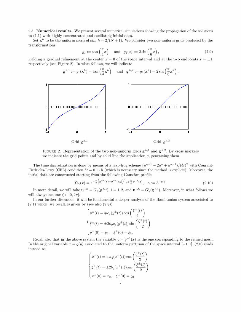


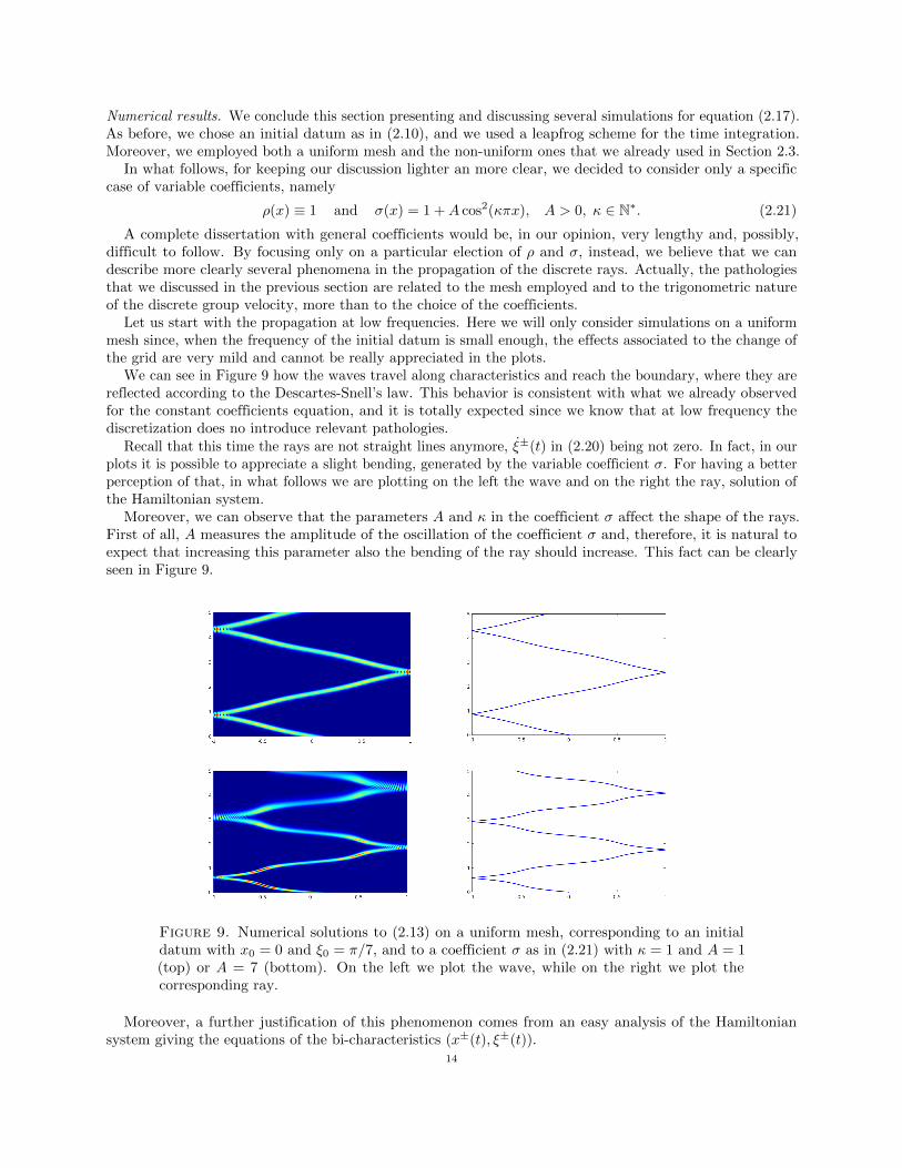


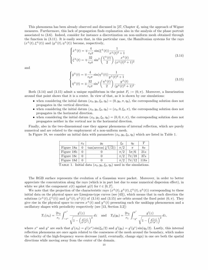


![Propagation of one and two-dimensional discrete waves …...upper part ˘2[ˇ;2ˇ] what would actually correspond to ˘2[ ˇ;0]. 15/42 Introduction One-dimensional wave equation Two-dimensional](https://static.documents.pub/doc/80x56/6119399ac713d9462912df7e/propagation-of-one-and-two-dimensional-discrete-waves-upper-part-22.jpg)


