Properties of a Family of Generalized NCP-Functions

and a Derivative Free Algorithm for Complementarity

Problems

Sheng-Long Hu

Department of Mathematics

School of Science, Tianjin University

Tianjin 300072, P.R. China

Zheng-Hai Huang ∗

Department of Mathematics

School of Science, Tianjin University

Tianjin 300072, P.R. China

Email: huangzhenghai@tju.edu.cn

Jein-Shan Chen †

Department of Mathematics

National Taiwan Normal University

Taipei, Taiwan 11677

Email: jschen@math.ntnu.edu.tw

September 7, 2008; Revised: October 24, 2008

∗Corresponding Author. The author’s work is partially supported by the National Natural ScienceFoundation of China (Grant No. 10571134 and No. 10871144) and the Natural Science Foundation ofTianjin (Grant No. 07JCYBJC05200).

†Member of Mathematics Division, National Center for Theoretical Sciences, Taipei Office. The author’swork is partially supported by National Science Council of Taiwan.

1

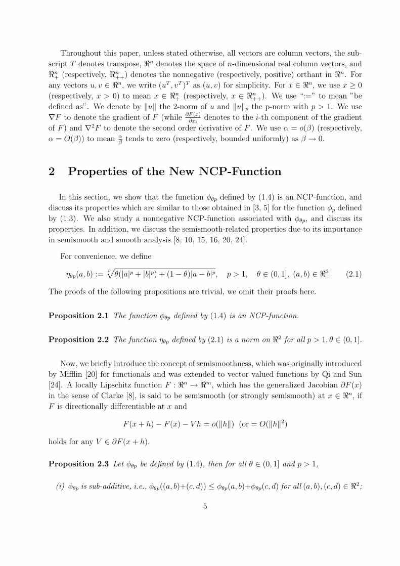
Abstract

In this paper, we propose a new family of NCP-functions and the corresponding meritfunctions, which are the generalization of some popular NCP-functions and the relatedmerit functions. We show that the new NCP-functions and the corresponding meritfunctions possess a system of favorite properties. Specially, we show that the newNCP-functions are strongly semismooth, Lipschitz continuous, and continuously dif-ferentiable; and that the corresponding merit functions have SC1 property (i.e., theyare continuously differentiable and their gradients are semismooth) and LC1 property(i.e., they are continuously differentiable and their gradients are Lipschitz continuous)under suitable assumptions. Based on the new NCP-functions and the correspondingmerit functions, we investigate a derivative free algorithm for the nonlinear comple-mentarity problem and discuss its global convergence. Some preliminary numericalresults are reported.

Key words: Complementarity problem, NCP-function, merit function, derivativefree algorithm.

AMS subject classifications (2000): 90C33, 90C56, 65K10.

2

1 Introduction

In the last decades, people have put a lot of their energy and attention on the com-

plementarity problem due to its various applications in operation research, economics, and

engineering (see, for examples, [10, 13, 23]). The nonlinear complementarity problem (NCP)

is to find a point x ∈ <n such that

x ≥ 0, F (x) ≥ 0, xT F (x) = 0, (1.1)

where F : <n → <n is a continuously differentiable mapping with F := (F1, F2, . . . , Fn)T .

Many solution methods have been developed to solve NCP (1.1), for examples, [3, 5, 13,

14, 15, 16, 17, 19, 23, 27, 28]. For more details, please refers to the excellent monograph

[9]. One of the most popular methods is to reformulate the NCP (1.1) as a unconstrained

optimization problem and then to solve the reformulated problem by the unconstrained

optimization technique. This kind of methods is called the merit function method, where

the merit function is generally constructed by some NCP-function.

Definition 1.1 A function φ : <2 → < is called an NCP-function [2, 18, 25, 26], if it

satisfies

φ(a, b) = 0 ⇐⇒ a ≥ 0, b ≥ 0, ab = 0.

Furthermore, if φ(a, b) ≥ 0 for all (a, b) ∈ <2 then the NCP-function φ is called a nonnegative

NCP-function. In addition, if a function Ψ : <n → < is nonnegative and Ψ(x) = 0 if and

only if x solves the NCP, then Ψ is called a merit function for the NCP.

If φ is an NCP-function, then it is easy to see that the function Ψ : <n → < defined

by Ψ(x) :=∑n

i=1 φ2(xi, Fi(x)) is a merit function for the NCP. Thus, finding a solution

of the NCP is equivalent to finding a global minimum of the unconstrained minimization

minx∈<nΨ(x) with optimal value 0.

Many NCP-functions have been proposed in the literature. Among them, the FB function

is one of the most popular NCP-functions, which is defined by

φ(a, b) :=√

a2 + b2 − a− b, ∀(a, b) ∈ <2.

One of the main generalization of FB function was given by Kanzow and Kleinmichel [18]:

φθ(a, b) :=√

(a− b)2 + θab− a− b, θ ∈ (0, 4), ∀(a, b) ∈ <2. (1.2)

Another main generalization was given by Chen and Pan [5]:

φp(a, b) :=p√|a|p + |b|p − a− b, p ∈ (1,∞), ∀(a, b) ∈ <2. (1.3)

3

It has been proved in [3, 4, 5, 6, 18, 22] that the functions φθ given in (1.2) and φp given

in (1.3) possess a system of favorite properties, such as, strong semismoothness, Lipschitz

continuity, and continuous differentiability. It has also been proved that the corresponding

merit functions of φθ and φp have SC1 property (i.e., they are continuously differentiable and

their gradients are semismooth) and LC1 property (i.e., they are continuously differentiable

and their gradients are Lipschitz continuous) under suitable assumptions.

Motivated by Kanzow and Kleinmichel [18] and Chen and Pan [5], we introduce in this

paper the following functions:

φθp(a, b) :=p√

θ(|a|p + |b|p) + (1− θ)|a− b|p − a− b, p > 1, θ ∈ (0, 1], (a, b) ∈ <2. (1.4)

and

Ψθp(x) :=1

2

n∑i=1

φ2θp(xi, Fi(x)). (1.5)

Is the function φθp an NCP-function? If it is, do the functions given by (1.4) and (1.5) have

the same properties as those known functions mentioned above? Furthermore, how is the

numerical behavior of the merit function methods based on the functions defined by (1.4) and

(1.5)?

In this paper, we will answer the questions mentioned above partly. Firstly, we show that

the function φθp defined by (1.4) is an NCP-function; and discuss some favorite properties of

the NCP-function (1.4) and its nonnegative NCP-function, including strong semismoothness,

Lipschitz continuity, and continuous differentiability. Since the function φθp defined by (1.4)

is an NCP-function, it follows that the function Ψθp defined by (1.5) is a merit function

associated to the NCP-function φθp. We also show that the merit function Ψθp has SC1

property and LC1 property. Secondly, we investigate a derivative free method based on

the functions defined by (1.4) and (1.5) and show its global convergence. (Note: usually

the nonsmooth Newton method is faster than the derivative free method for solving NCPs.

However, the derivative free algorithm may overcome the case where strong conditions are

sometimes needed to guarantee that the Jacobian of the merit function is nonsingular or

very expensive to compute.) Thirdly, we report the preliminary numerical results for test

problems from MCPLIB. The preliminary numerical results show, on the average, that the

algorithm works better when θ = 1 (according to the FB-type function), θ = 0.9 and

θ = 0.25, and when p = 1.1 or p = 2 or p = 20 generally.

The rest of this paper are organized as follows. Various properties of the new NCP-

function (1.4) and the nonnegative NCP-function associated to (1.4) are established in the

next section. In Section 3, some properties of the merit function defined by (1.5) are an-

alyzed. In Section 4, we investigate a derivative free algorithm for the NCP and show its

global convergence. Some preliminary numerical results are reported in Section 5 and final

conclusions are given in the last section.

4

Throughout this paper, unless stated otherwise, all vectors are column vectors, the sub-

script T denotes transpose, <n denotes the space of n-dimensional real column vectors, and

<n+ (respectively, <n

++) denotes the nonnegative (respectively, positive) orthant in <n. For

any vectors u, v ∈ <n, we write (uT , vT )T as (u, v) for simplicity. For x ∈ <n, we use x ≥ 0

(respectively, x > 0) to mean x ∈ <n+ (respectively, x ∈ <n

++). We use “:=” to mean ”be

defined as”. We denote by ‖u‖ the 2-norm of u and ‖u‖p the p-norm with p > 1. We use

∇F to denote the gradient of F (while ∂F (x)∂xi

denotes to the i-th component of the gradient

of F ) and ∇2F to denote the second order derivative of F . We use α = o(β) (respectively,

α = O(β)) to mean αβ

tends to zero (respectively, bounded uniformly) as β → 0.

2 Properties of the New NCP-Function

In this section, we show that the function φθp defined by (1.4) is an NCP-function, and

discuss its properties which are similar to those obtained in [3, 5] for the function φp defined

by (1.3). We also study a nonnegative NCP-function associated with φθp, and discuss its

properties. In addition, we discuss the semismooth-related properties due to its importance

in semismooth and smooth analysis [8, 10, 15, 16, 20, 24].

For convenience, we define

ηθp(a, b) :=p√

θ(|a|p + |b|p) + (1− θ)|a− b|p, p > 1, θ ∈ (0, 1], (a, b) ∈ <2. (2.1)

The proofs of the following propositions are trivial, we omit their proofs here.

Proposition 2.1 The function φθp defined by (1.4) is an NCP-function.

Proposition 2.2 The function ηθp defined by (2.1) is a norm on <2 for all p > 1, θ ∈ (0, 1].

Now, we briefly introduce the concept of semismoothness, which was originally introduced

by Mifflin [20] for functionals and was extended to vector valued functions by Qi and Sun

[24]. A locally Lipschitz function F : <n → <m, which has the generalized Jacobian ∂F (x)

in the sense of Clarke [8], is said to be semismooth (or strongly semismooth) at x ∈ <n, if

F is directionally differentiable at x and

F (x + h)− F (x)− V h = o(‖h‖) (or = O(‖h‖2)

holds for any V ∈ ∂F (x + h).

Proposition 2.3 Let φθp be defined by (1.4), then for all θ ∈ (0, 1] and p > 1,

(i) φθp is sub-additive, i.e., φθp((a, b)+(c, d)) ≤ φθp(a, b)+φθp(c, d) for all (a, b), (c, d) ∈ <2;

5

(ii) φθp is positive homogenous, i.e., φθp(α(a, b)) = αφθp(a, b) for all (a, b) ∈ <2 and α > 0;

(iii) φθp is a convex function on <2, i.e., φθp(α(a, b) + (1 − α)(c, d)) ≤ αφθp(a, b) + (1 −α)φθp(c, d) for all (a, b), (c, d) ∈ <2 and α ∈ [0, 1];

(iv) φθp is Lipschitz continuous on <2;

(v) φθp is continuously differentiable on <2\{(0, 0)};

(vi) φθp is strongly semismooth on <2.

Proof. By using φθp((a, b)) = ηθp(a, b) − (a + b) and Proposition 2.2, we can obtain that

the results (i), (ii), and (iii) hold.

Consider the result (iv). Since ηθp is a norm on <2 from Proposition 2.2 and any two

norms in finite dimensional space are equivalent, it follows that there exists a positive con-

stant κ such that

ηθp(a, b) ≤ κ‖(a, b)‖, ∀(a, b) ∈ <2,

where ‖ · ‖ represents the Euclidean norm on <2. Hence, for all (a, b), (c, d) ∈ <2,

|φθp(a, b)− φθp(c, d)| = |ηθp(a, b)− (a + b)− ηθp(c, d) + (c + d)|≤ |ηθp(a, b)− ηθp(c, d)|+ |a− c|+ |b− d|≤ ηθp(a− c, b− d) +

√2‖(a− c, b− d)‖

≤ κ‖(a− c, b− d)‖+√

2‖(a− c, b− d)‖= (κ +

√2)‖(a− c, b− d)‖.

Hence, φθp is Lipschitz continuous with Lipschitz constant κ+√

2, i.e., the result (iv) holds.

Consider the result (v). If (a, b) 6= (0, 0), then ηθp(a, b) 6= 0 by Proposition 2.2. By a

direct calculation, we get

∂φθp(a, b)

∂a=

θsgn(a)|a|p−1 + (1− θ)sgn(a− b)|a− b|p−1

ηθp(a, b)p−1− 1; (2.2)

∂φθp(a, b)

∂b=

θsgn(b)|b|p−1 − (1− θ)sgn(a− b)|a− b|p−1

ηθp(a, b)p−1− 1, (2.3)

where sgn(·) is the symbol function. It is easy to see from (2.2) and (2.3) that the result

(v) holds.

Consider the result (vi). Since φθp is a convex function by the result (iii), we get that it

is a semismooth function. Noticing that φθp is continuously differentiable except (0, 0), it is

6

sufficient to prove that it is strongly semismooth at (0, 0). For any (h, k) ∈ <2\{(0, 0)}, φθp

is differentiable at (h, k), and hence, ∇φθp(h, k) =(

∂φθp(h,k)

∂a,

∂φθp(h,k)

∂b

)T

. So,

φθp((0, 0) + (h, k))− φθp(0, 0)−(

∂φθp(h, k)

∂a,∂φθp(h, k)

∂b

)(h

k

)

=p√

θ(|h|p + |k|p) + (1− θ)|h− k|p − (h + k)

−(sgn(h)|h|p−1 + sgn(h− k)|h− k|p−1

ηθp(h, k)p−1− 1)h

−(sgn(k)|k|p−1 − sgn(h− k)|h− k|p−1

ηθp(h, k)p−1− 1)k

=p√

θ(|h|p + |k|p) + (1− θ)|h− k|p

−sgn(h)|h|p−1h + sgn(k)|k|p−1k + sgn(h− k)|h− k|p−1(h− k)

ηθp(h, k)p−1

=p√

θ(|h|p + |k|p) + (1− θ)|h− k|p − |h|p + |k|p + |h− k|pηθp(h, k)p−1

= ηθp(h, k)− |h|p + |k|p + |h− k|pηθp(h, k)p−1

=ηθp(h, k)p − (|h|p + |k|p + |h− k|p)

ηθp(h, k)p−1

= 0

= O(‖(h, k)‖2).

Thus, we obtain that φθp is strongly semismooth.

We complete the proof. 2

Proposition 2.4 Let φθp be defined by (1.4) and {(ak, bk)} ⊆ <2. Then, |φθp(ak, bk)| → ∞

if one of the following conditions is satisfied.

(i). ak → −∞; (ii). bk → −∞; (iii). ak →∞ and bk →∞.

Proof. (i) Suppose that ak → −∞. If {bk} is bounded from above, then the result holds

trivially. When bk →∞, we have −ak > 0 and bk > 0 for all k sufficiently large, and hence,

p√

θ(|ak|p + |bk|p) + (1− θ)|ak − bk|p − bk ≥ p√

θ|bk|p + (1− θ)|bk|p − bk = 0.

This, together with −ak →∞ and the definition of φθp, implies that the result holds.

(ii) For the case of bk → −∞, a similar analysis yields the result of the proposition.

(iii) Suppose that ak →∞ and bk →∞. Since p > 1 and θ ∈ (0, 1], we have (1− θ)|ak−bk|p ≤ (1− θ)(|ak|p + |bk|p) for all sufficiently large k. Thus, for all sufficiently large k,

p√

θ(|ak|p + |bk|p) + (1− θ)|ak − bk|p ≤ p√|ak|p + |bk|p,

7

and hence,

(ak + bk)− p√

θ(|ak|p + |bk|p) + (1− θ)|ak − bk|p ≥ (ak + bk)− p√|ak|p + |bk|p.

By [5, Lemma 3.1] we know that (ak + bk) − p√|ak|p + |bk|p → ∞ as k → ∞ when the

condition (iii) is satisfied. Thus, we obtain that

|φθp(ak, bk)| = (ak + bk)− p

√θ(|ak|p + |bk|p) + (1− θ)|ak − bk|p →∞

as k →∞, which completes the proof. 2

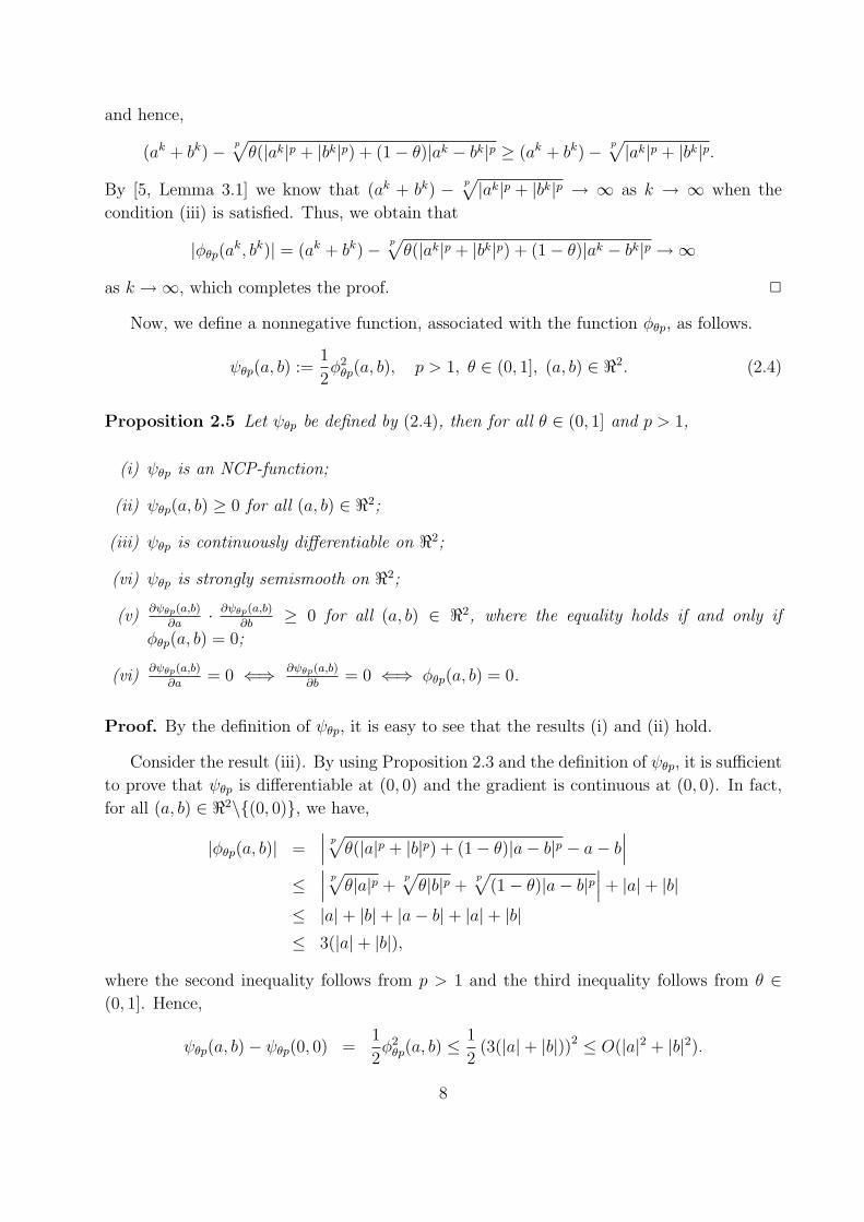
Now, we define a nonnegative function, associated with the function φθp, as follows.

ψθp(a, b) :=1

2φ2

θp(a, b), p > 1, θ ∈ (0, 1], (a, b) ∈ <2. (2.4)

Proposition 2.5 Let ψθp be defined by (2.4), then for all θ ∈ (0, 1] and p > 1,

(i) ψθp is an NCP-function;

(ii) ψθp(a, b) ≥ 0 for all (a, b) ∈ <2;

(iii) ψθp is continuously differentiable on <2;

(vi) ψθp is strongly semismooth on <2;

(v)∂ψθp(a,b)

∂a· ∂ψθp(a,b)

∂b≥ 0 for all (a, b) ∈ <2, where the equality holds if and only if

φθp(a, b) = 0;

(vi)∂ψθp(a,b)

∂a= 0 ⇐⇒ ∂ψθp(a,b)

∂b= 0 ⇐⇒ φθp(a, b) = 0.

Proof. By the definition of ψθp, it is easy to see that the results (i) and (ii) hold.

Consider the result (iii). By using Proposition 2.3 and the definition of ψθp, it is sufficient

to prove that ψθp is differentiable at (0, 0) and the gradient is continuous at (0, 0). In fact,

for all (a, b) ∈ <2\{(0, 0)}, we have,

|φθp(a, b)| =∣∣∣ p√

θ(|a|p + |b|p) + (1− θ)|a− b|p − a− b∣∣∣

≤∣∣∣ p√

θ|a|p +p√

θ|b|p +p√

(1− θ)|a− b|p∣∣∣ + |a|+ |b|

≤ |a|+ |b|+ |a− b|+ |a|+ |b|≤ 3(|a|+ |b|),

where the second inequality follows from p > 1 and the third inequality follows from θ ∈(0, 1]. Hence,

ψθp(a, b)− ψθp(0, 0) =1

2φ2

θp(a, b) ≤ 1

2(3(|a|+ |b|))2 ≤ O(|a|2 + |b|2).

8

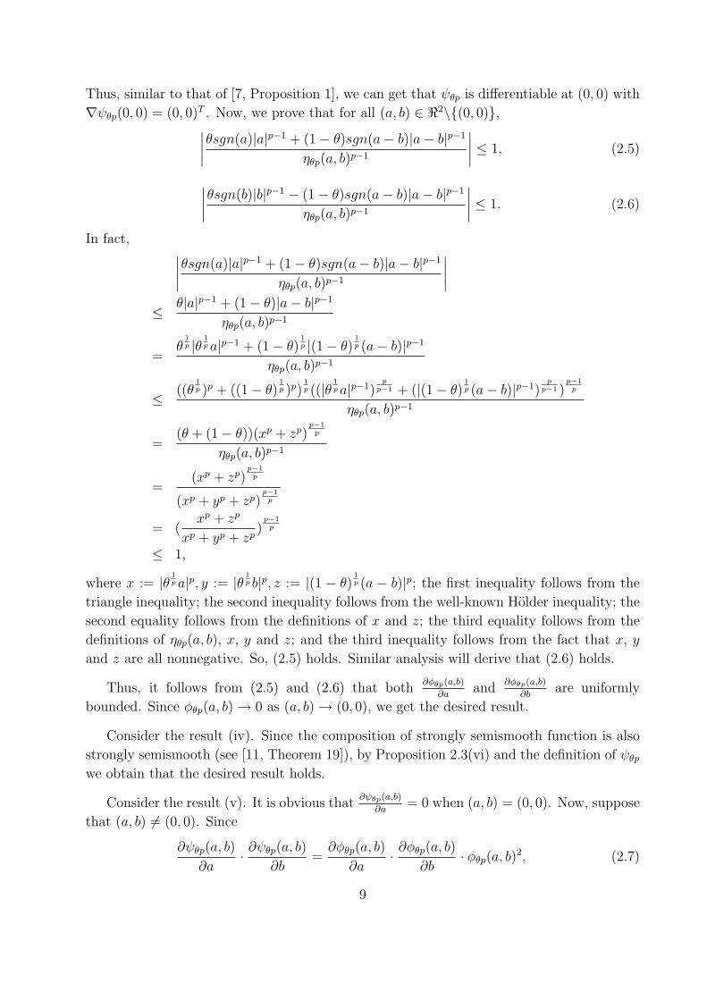
Thus, similar to that of [7, Proposition 1], we can get that ψθp is differentiable at (0, 0) with

∇ψθp(0, 0) = (0, 0)T . Now, we prove that for all (a, b) ∈ <2\{(0, 0)},∣∣∣∣θsgn(a)|a|p−1 + (1− θ)sgn(a− b)|a− b|p−1

ηθp(a, b)p−1

∣∣∣∣ ≤ 1, (2.5)

∣∣∣∣θsgn(b)|b|p−1 − (1− θ)sgn(a− b)|a− b|p−1

ηθp(a, b)p−1

∣∣∣∣ ≤ 1. (2.6)

In fact,∣∣∣∣θsgn(a)|a|p−1 + (1− θ)sgn(a− b)|a− b|p−1

ηθp(a, b)p−1

∣∣∣∣

≤ θ|a|p−1 + (1− θ)|a− b|p−1

ηθp(a, b)p−1

=θ

1p |θ 1

p a|p−1 + (1− θ)1p |(1− θ)

1p (a− b)|p−1

ηθp(a, b)p−1

≤ ((θ1p )p + ((1− θ)

1p )p)

1p ((|θ 1

p a|p−1)p

p−1 + (|(1− θ)1p (a− b)|p−1)

pp−1 )

p−1p

ηθp(a, b)p−1

=(θ + (1− θ))(xp + zp)

p−1p

ηθp(a, b)p−1

=(xp + zp)

p−1p

(xp + yp + zp)p−1

p

= (xp + zp

xp + yp + zp)

p−1p

≤ 1,

where x := |θ 1p a|p, y := |θ 1

p b|p, z := |(1 − θ)1p (a − b)|p; the first inequality follows from the

triangle inequality; the second inequality follows from the well-known Holder inequality; the

second equality follows from the definitions of x and z; the third equality follows from the

definitions of ηθp(a, b), x, y and z; and the third inequality follows from the fact that x, y

and z are all nonnegative. So, (2.5) holds. Similar analysis will derive that (2.6) holds.

Thus, it follows from (2.5) and (2.6) that both∂φθp(a,b)

∂aand

∂φθp(a,b)

∂bare uniformly

bounded. Since φθp(a, b) → 0 as (a, b) → (0, 0), we get the desired result.

Consider the result (iv). Since the composition of strongly semismooth function is also

strongly semismooth (see [11, Theorem 19]), by Proposition 2.3(vi) and the definition of ψθp

we obtain that the desired result holds.

Consider the result (v). It is obvious that∂ψθp(a,b)

∂a= 0 when (a, b) = (0, 0). Now, suppose

that (a, b) 6= (0, 0). Since

∂ψθp(a, b)

∂a· ∂ψθp(a, b)

∂b=

∂φθp(a, b)

∂a· ∂φθp(a, b)

∂b· φθp(a, b)2, (2.7)

9

by (2.2), (2.3), (2.5), and (2.6), we obtain that∂φθp(a,b)

∂a≤ 0 and

∂φθp(a,b)

∂b≤ 0 for all (a, b) ∈ <2,

that is, the first result of (v) holds. In addition, from (2.7) it is obvious that the sufficient

condition of the second result of (v) holds. Now, we suppose that∂ψθp(a,b)

∂a· ∂ψθp(a,b)

∂b= 0.

Then, it is sufficient to prove that φθp(a, b) = 0 when∂φθp(a,b)

∂a· ∂φθp(a,b)

∂b= 0. Suppose that

∂φθp(a,b)

∂a= 0 without loss of generality. From the proof of (iii) in this proposition, it is easy

to see that it must be y = 0, and hence, b = 0. After a simple symbol discussion for (2.2),

we may get a ≥ 0. Hence φθp(a, b) = 0 by Proposition 2.1. So, the result (v) holds.

Consider the result (vi). Since

∂ψθp(a, b)

∂a=

∂φθp(a, b)

∂aφθp(a, b),

∂ψθp(a, b)

∂b=

∂φθp(a, b)

∂bφθp(a, b),

the result (vi) is immediately satisfied from the above analysis.

We complete the proof. 2

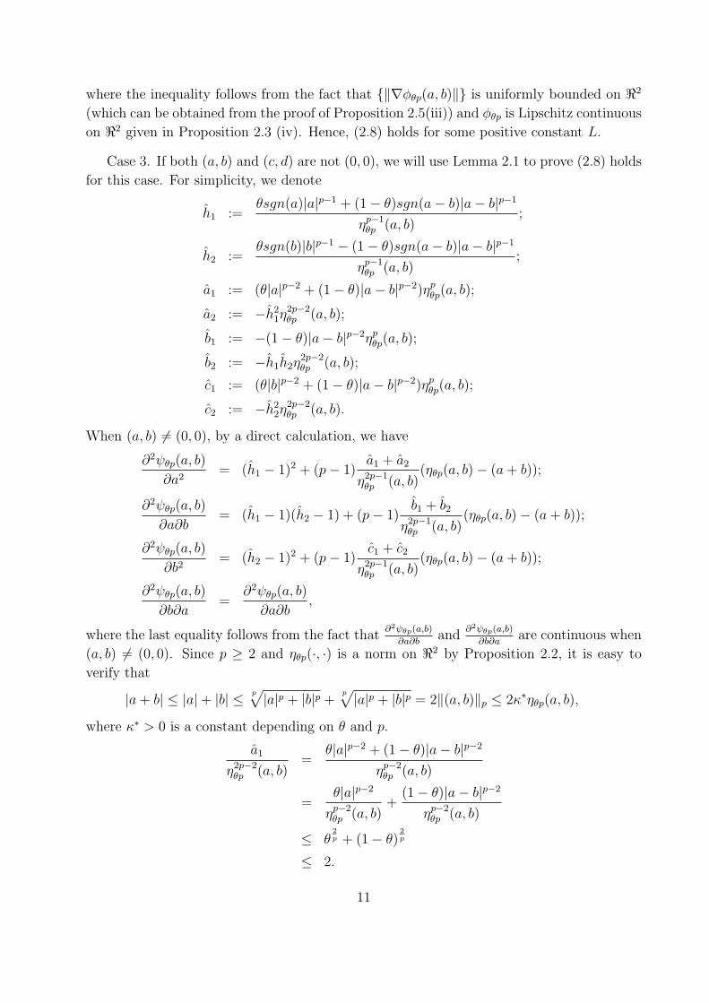
Lemma 2.1 [21, Theorem 3.3.5] If f : D ⊆ <n → <m has a second derivative at each point

of a convex set D0 ⊆ D, then ‖∇f(y)−∇f(x)‖ ≤ sup0≤t≤1 ‖∇2f(x + t(y − x))‖ · ‖y − x‖.

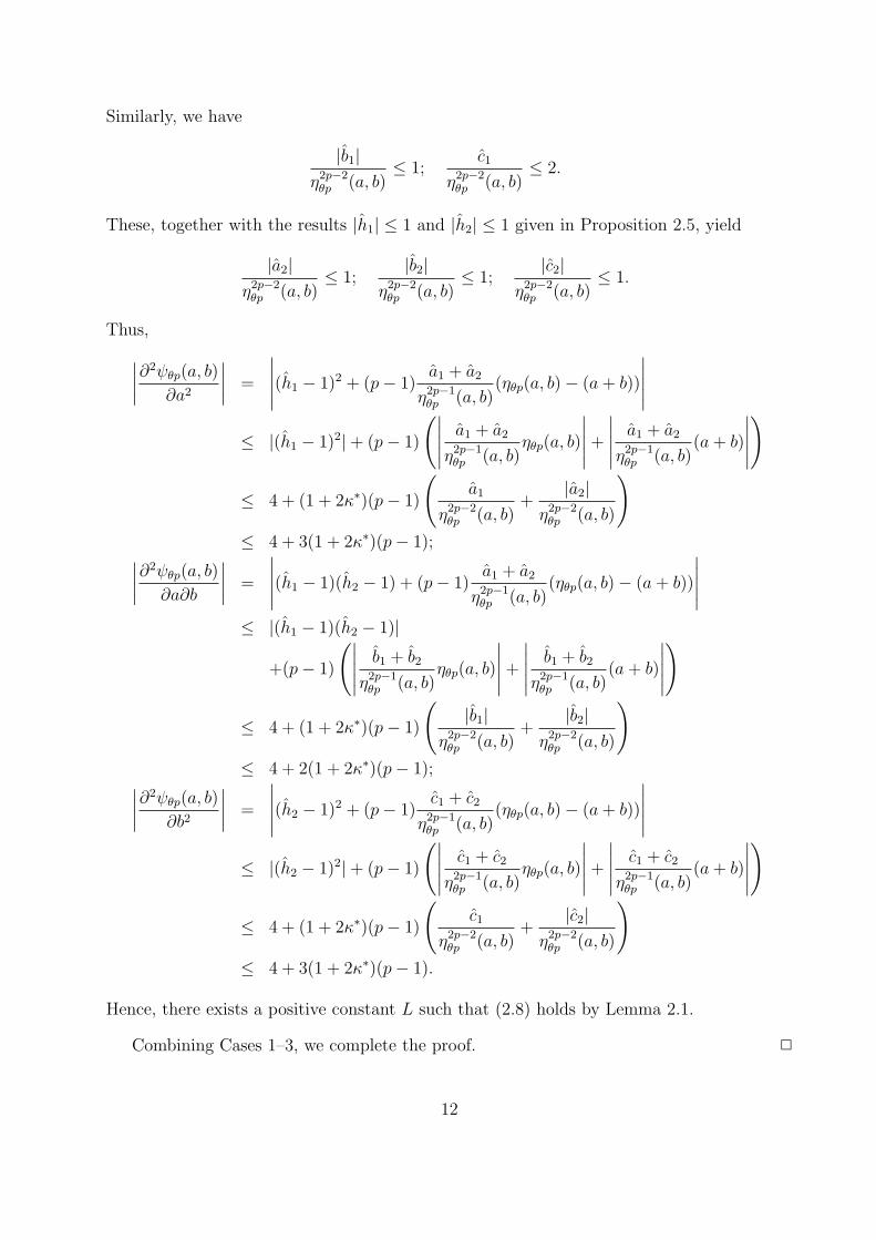
Theorem 2.1 The gradient function of the function ψθp defined by (2.4) with p ≥ 2, θ ∈(0, 1] is Lipschitz continuous, that is, there exists a positive constant L such that

‖∇ψθp(a, b)−∇ψθp(c, d)‖ ≤ L‖(a, b)− (c, d)‖ (2.8)

holds for all (a, b), (c, d) ∈ <2.

Proof. It follows from the definition of ψθp and the proof of Proposition 2.5(iii) that

∇ψθp(a, b) = ∇φθp(a, b)φθp(a, b) when (a, b) 6= (0, 0), and ∇ψθp(0, 0) = (0, 0)T . From Propo-

sition 2.5(iii) we know that ψθp is continuous differentiable. The proof is divided into the

following three cases.

Case 1. If (a, b) = (c, d) = (0, 0), it follows from Proposition 2.5 that ∇ψθp(0, 0) = (0, 0),

and hence, (2.8) holds for all positive number L.

Case 2. Consider the case that one of (a, b) and (c, d) is (0, 0), but not all. We assume

that (a, b) 6= (0, 0) and (c, d) = (0, 0) without loss of generality. Then,

‖∇ψθp(a, b)−∇ψθp(c, d)‖ = ‖∇ψθp(a, b)− (0, 0)‖= ‖∇φθp(a, b)φθp(a, b)− (0, 0)‖= ‖∇φθp(a, b)‖φθp(a, b)

= ‖∇φθp(a, b)‖|φθp(a, b)− φθp(0, 0)|≤ L‖(a, b)− (0, 0)‖,

10

where the inequality follows from the fact that {‖∇φθp(a, b)‖} is uniformly bounded on <2

(which can be obtained from the proof of Proposition 2.5(iii)) and φθp is Lipschitz continuous

on <2 given in Proposition 2.3 (iv). Hence, (2.8) holds for some positive constant L.

Case 3. If both (a, b) and (c, d) are not (0, 0), we will use Lemma 2.1 to prove (2.8) holds

for this case. For simplicity, we denote

h1 :=θsgn(a)|a|p−1 + (1− θ)sgn(a− b)|a− b|p−1

ηp−1θp (a, b)

;

h2 :=θsgn(b)|b|p−1 − (1− θ)sgn(a− b)|a− b|p−1

ηp−1θp (a, b)

;

a1 := (θ|a|p−2 + (1− θ)|a− b|p−2)ηpθp(a, b);

a2 := −h21η

2p−2θp (a, b);

b1 := −(1− θ)|a− b|p−2ηpθp(a, b);

b2 := −h1h2η2p−2θp (a, b);

c1 := (θ|b|p−2 + (1− θ)|a− b|p−2)ηpθp(a, b);

c2 := −h22η

2p−2θp (a, b).

When (a, b) 6= (0, 0), by a direct calculation, we have

∂2ψθp(a, b)

∂a2= (h1 − 1)2 + (p− 1)

a1 + a2

η2p−1θp (a, b)

(ηθp(a, b)− (a + b));

∂2ψθp(a, b)

∂a∂b= (h1 − 1)(h2 − 1) + (p− 1)

b1 + b2

η2p−1θp (a, b)

(ηθp(a, b)− (a + b));

∂2ψθp(a, b)

∂b2= (h2 − 1)2 + (p− 1)

c1 + c2

η2p−1θp (a, b)

(ηθp(a, b)− (a + b));

∂2ψθp(a, b)

∂b∂a=

∂2ψθp(a, b)

∂a∂b,

where the last equality follows from the fact that∂2ψθp(a,b)

∂a∂band

∂2ψθp(a,b)

∂b∂aare continuous when

(a, b) 6= (0, 0). Since p ≥ 2 and ηθp(·, ·) is a norm on <2 by Proposition 2.2, it is easy to

verify that

|a + b| ≤ |a|+ |b| ≤ p√|a|p + |b|p +

p√|a|p + |b|p = 2‖(a, b)‖p ≤ 2κ∗ηθp(a, b),

where κ∗ > 0 is a constant depending on θ and p.

a1

η2p−2θp (a, b)

=θ|a|p−2 + (1− θ)|a− b|p−2

ηp−2θp (a, b)

=θ|a|p−2

ηp−2θp (a, b)

+(1− θ)|a− b|p−2

ηp−2θp (a, b)

≤ θ2p + (1− θ)

2p

≤ 2.

11

Similarly, we have

|b1|η2p−2

θp (a, b)≤ 1;

c1

η2p−2θp (a, b)

≤ 2.

These, together with the results |h1| ≤ 1 and |h2| ≤ 1 given in Proposition 2.5, yield

|a2|η2p−2

θp (a, b)≤ 1;

|b2|η2p−2

θp (a, b)≤ 1;

|c2|η2p−2

θp (a, b)≤ 1.

Thus,

∣∣∣∣∂2ψθp(a, b)

∂a2

∣∣∣∣ =

∣∣∣∣∣(h1 − 1)2 + (p− 1)a1 + a2

η2p−1θp (a, b)

(ηθp(a, b)− (a + b))

∣∣∣∣∣

≤ |(h1 − 1)2|+ (p− 1)

(∣∣∣∣∣a1 + a2

η2p−1θp (a, b)

ηθp(a, b)

∣∣∣∣∣ +

∣∣∣∣∣a1 + a2

η2p−1θp (a, b)

(a + b)

∣∣∣∣∣

)

≤ 4 + (1 + 2κ∗)(p− 1)

(a1

η2p−2θp (a, b)

+|a2|

η2p−2θp (a, b)

)

≤ 4 + 3(1 + 2κ∗)(p− 1);∣∣∣∣∂2ψθp(a, b)

∂a∂b

∣∣∣∣ =

∣∣∣∣∣(h1 − 1)(h2 − 1) + (p− 1)a1 + a2

η2p−1θp (a, b)

(ηθp(a, b)− (a + b))

∣∣∣∣∣≤ |(h1 − 1)(h2 − 1)|

+(p− 1)

(∣∣∣∣∣b1 + b2

η2p−1θp (a, b)

ηθp(a, b)

∣∣∣∣∣ +

∣∣∣∣∣b1 + b2

η2p−1θp (a, b)

(a + b)

∣∣∣∣∣

)

≤ 4 + (1 + 2κ∗)(p− 1)

(|b1|

η2p−2θp (a, b)

+|b2|

η2p−2θp (a, b)

)

≤ 4 + 2(1 + 2κ∗)(p− 1);∣∣∣∣∂2ψθp(a, b)

∂b2

∣∣∣∣ =

∣∣∣∣∣(h2 − 1)2 + (p− 1)c1 + c2

η2p−1θp (a, b)

(ηθp(a, b)− (a + b))

∣∣∣∣∣

≤ |(h2 − 1)2|+ (p− 1)

(∣∣∣∣∣c1 + c2

η2p−1θp (a, b)

ηθp(a, b)

∣∣∣∣∣ +

∣∣∣∣∣c1 + c2

η2p−1θp (a, b)

(a + b)

∣∣∣∣∣

)

≤ 4 + (1 + 2κ∗)(p− 1)

(c1

η2p−2θp (a, b)

+|c2|

η2p−2θp (a, b)

)

≤ 4 + 3(1 + 2κ∗)(p− 1).

Hence, there exists a positive constant L such that (2.8) holds by Lemma 2.1.

Combining Cases 1–3, we complete the proof. 2

12

Remark 2.1 It should be noted that ∇ψθp is not Lipschitz continuous for all θ ∈ (0, 1] when

p ∈ (1, 2). In fact, if we fixed θ = 1. For (a, b) 6= (0, 0) and (c, d) 6= (0, 0), we have

‖∇ψ1p(a, b)−∇ψ1p(c, d)‖= ‖∇φ1p(a, b)φ1p(a, b)−∇φ1p(c, d)φ1p(c, d)‖≥

∣∣∣∣sgn(a)|a|p−1

‖(a, b)‖p−1p

φ1p(a, b)− sgn(c)|c|p−1

‖(c, d)‖p−1p

φ1p(c, d) + φ1p(c, d)− φ1p(a, b)

∣∣∣∣

≥∣∣∣∣sgn(a)|a|p−1

‖(a, b)‖p−1p

φ1p(a, b)− sgn(c)|c|p−1

‖(c, d)‖p−1p

φ1p(c, d)

∣∣∣∣− |φ1p(c, d)− φ1p(a, b)|

≥∣∣∣∣sgn(a)|a|p−1

‖(a, b)‖p−1p

φ1p(a, b)− sgn(c)|c|p−1

‖(c, d)‖p−1p

φ1p(c, d)

∣∣∣∣− (κ +√

2)‖(c, d)− (a, b)‖,

where κ +√

2 is given in Proposition 2.3(iv). If we let (a, b) = (1,−n), (c, d) = (−1,−n)

with n ∈ (1,∞), we have

∣∣∣∣sgn(a)|a|p−1

‖(a, b)‖p−1p

φ1p(a, b)− sgn(c)|c|p−1

‖(c, d)‖p−1p

φ1p(c, d)

∣∣∣∣

=

p√1 + np + (n− 1)

(1 + np)(p−1)/p+

p√1 + np + (n + 1)

(1 + np)(p−1)/p

= 2

p√1 + np + n

(1 + np)(p−1)/p

≥ 4n

(1 + np)(p−1)/p

=4n2−pnp−1

(1 + np)(p−1)/p

=4n2−p

(1 + (1/n)p)(p−1)/p

≥ n2−p,

where the first and the second inequalities follow from 2 > p > 1 and n > 1. Since ‖(a, b)−(c, d)‖ = 2 and n ∈ (1,∞), form the above inequalities it is easy to verify that ∇ψ1p is not

Lipschitz continuous.

3 Properties of Merit Function

In this section, we consider the merit function for the NCP defined by (1.5), and then

discuss its several important properties. These properties provide the theoretical basis for

the algorithm we discussed in the next section. In addition, we also discuss the semismooth-

related properties of the merit function.

13

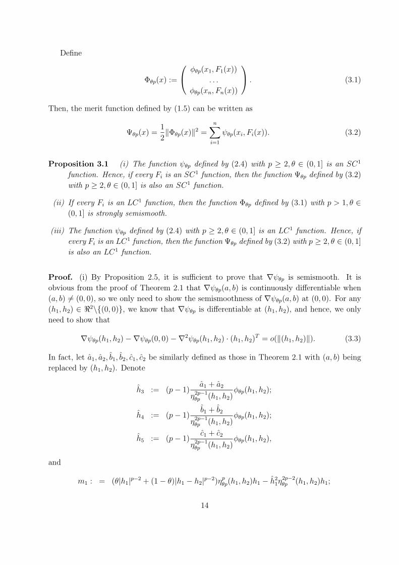
Define

Φθp(x) :=

φθp(x1, F1(x))

. . .

φθp(xn, Fn(x))

. (3.1)

Then, the merit function defined by (1.5) can be written as

Ψθp(x) =1

2‖Φθp(x)‖2 =

n∑i=1

ψθp(xi, Fi(x)). (3.2)

Proposition 3.1 (i) The function ψθp defined by (2.4) with p ≥ 2, θ ∈ (0, 1] is an SC1

function. Hence, if every Fi is an SC1 function, then the function Ψθp defined by (3.2)

with p ≥ 2, θ ∈ (0, 1] is also an SC1 function.

(ii) If every Fi is an LC1 function, then the function Φθp defined by (3.1) with p > 1, θ ∈(0, 1] is strongly semismooth.

(iii) The function ψθp defined by (2.4) with p ≥ 2, θ ∈ (0, 1] is an LC1 function. Hence, if

every Fi is an LC1 function, then the function Ψθp defined by (3.2) with p ≥ 2, θ ∈ (0, 1]

is also an LC1 function.

Proof. (i) By Proposition 2.5, it is sufficient to prove that ∇ψθp is semismooth. It is

obvious from the proof of Theorem 2.1 that ∇ψθp(a, b) is continuously differentiable when

(a, b) 6= (0, 0), so we only need to show the semismoothness of ∇ψθp(a, b) at (0, 0). For any

(h1, h2) ∈ <2\{(0, 0)}, we know that ∇ψθp is differentiable at (h1, h2), and hence, we only

need to show that

∇ψθp(h1, h2)−∇ψθp(0, 0)−∇2ψθp(h1, h2) · (h1, h2)T = o(‖(h1, h2)‖). (3.3)

In fact, let a1, a2, b1, b2, c1, c2 be similarly defined as those in Theorem 2.1 with (a, b) being

replaced by (h1, h2). Denote

h3 := (p− 1)a1 + a2

η2p−1θp (h1, h2)

φθp(h1, h2);

h4 := (p− 1)b1 + b2

η2p−1θp (h1, h2)

φθp(h1, h2);

h5 := (p− 1)c1 + c2

η2p−1θp (h1, h2)

φθp(h1, h2),

and

m1 : = (θ|h1|p−2 + (1− θ)|h1 − h2|p−2)ηpθp(h1, h2)h1 − h2

1η2p−2θp (h1, h2)h1;

14

m2 : = (1− θ)|h1 − h2|p−2ηpθp(h1, h2)h2 + h1h2η

2p−2θp (h1, h2)h2;

m3 : = (θ|h1|p−2 + (1− θ)|h1 − h2|p−2)ηpθp(h1, h2)h1

−(1− θ)|h1 − h2|p−2ηpθp(h1, h2)h2;

m4 : = h1h2η2p−2θp (h1, h2)h2 + h2

1η2p−2θp (h1, h2)h1;

m5 : = (θsgn(h1)|h1|p−1 + (1− θ)sgn(h1 − h2)|h1 − h2|p−1)ηpθp(h1, h2);

m6 : = h1h2η2p−2θp (h1, h2)h2 + h2

1η2p−2θp (h1, h2)h1.

Then,

(H1

H2

):=

(h1 − 1

h2 − 1

)· φθp(h1, h2)−

(0

0

)

−(

(h1 − 1)2 + h3 (h1 − 1)(h2 − 1) + h4

(h1 − 1)(h2 − 1) + h4 (h2 − 1)2 + h5

)·(

h1

h2

).

and hence,

H1 = (h1 − 1)φθp(h1, h2)− ((h1 − 1)2 + h3)h1 − ((h1 − 1)(h2 − 1) + h4)h2

= (h1 − 1)φθp(h1, h2)− h3h1 − h4h2 − (h1 − 1)((h1 − 1)h1 + (h2 − 1)h2)

= (h1 − 1)φθp(h1, h2)− h3h1 − h4h2 − (h1 − 1)φθp(h1, h2)

= −(p− 1)

(a1 + a2

η2p−1θp (h1, h2)

h1 +b1 + b2

η2p−1θp (h1, h2)

h2

)φθp(h1, h2)

= −(p− 1)φθp(h1, h2)

(m1 −m2

η2p−1θp (h1, h2)

)

= −(p− 1)φθp(h1, h2)

(m3 −m4

η2p−1θp (h1, h2)

)

= −(p− 1)φθp(h1, h2)

(m5 −m6

η2p−1θp (h1, h2)

)

= −(p− 1)φθp(h1, h2)

(h1 − h1

h1h1 + h2h2

ηθp(h1, h2)

)

= −(p− 1)φθp(h1, h2)(h1 − h1)

= 0,

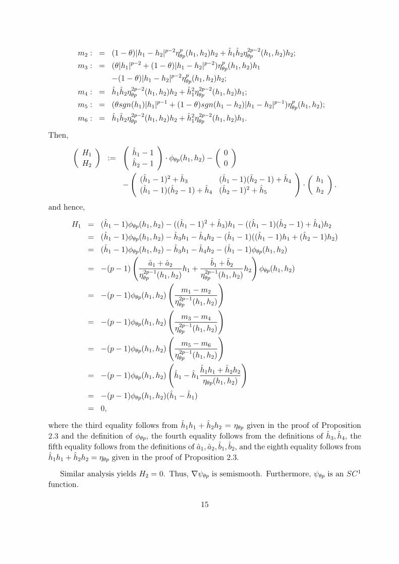
where the third equality follows from h1h1 + h2h2 = ηθp given in the proof of Proposition

2.3 and the definition of φθp, the fourth equality follows from the definitions of h3, h4, the

fifth equality follows from the definitions of a1, a2, b1, b2, and the eighth equality follows from

h1h1 + h2h2 = ηθp given in the proof of Proposition 2.3.

Similar analysis yields H2 = 0. Thus, ∇ψθp is semismooth. Furthermore, ψθp is an SC1

function.

15

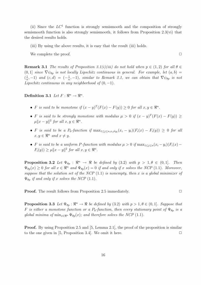
(ii) Since the LC1 function is strongly semismooth and the composition of strongly

semismooth function is also strongly semismooth, it follows from Proposition 2.3(vi) that

the desired results holds.

(iii) By using the above results, it is easy that the result (iii) holds.

We complete the proof. 2

Remark 3.1 The results of Proposition 3.1(i)(iii) do not hold when p ∈ (1, 2) for all θ ∈(0, 1] since ∇ψθp is not locally Lipschitz continuous in general. For example, let (a, b) =

( 1n,−1) and (c, d) = (− 1

n,−1), similar to Remark 2.1, we can obtain that ∇ψθp is not

Lipschitz continuous in any neighborhood of (0,−1).

Definition 3.1 Let F : <n → <n.

• F is said to be monotone if (x− y)T (F (x)− F (y)) ≥ 0 for all x, y ∈ <n.

• F is said to be strongly monotone with modulus µ > 0 if (x − y)T (F (x) − F (y)) ≥µ‖x− y‖2 for all x, y ∈ <n.

• F is said to be a P0-function if max1≤j≤n,xi 6=yi(xi − yi)(Fi(x) − Fi(y)) ≥ 0 for all

x, y ∈ <n and x 6= y.

• F is said to be a uniform P -function with modulus µ > 0 if max1≤j≤n(xi− yi)(Fi(x)−Fi(y)) ≥ µ‖x− y‖2 for all x, y ∈ <n.

Proposition 3.2 Let Ψθp : <n → < be defined by (3.2) with p > 1, θ ∈ (0, 1]. Then

Ψθp(x) ≥ 0 for all x ∈ <n and Ψθp(x) = 0 if and only if x solves the NCP (1.1). Moreover,

suppose that the solution set of the NCP (1.1) is nonempty, then x is a global minimizer of

Ψθp if and only if x solves the NCP (1.1).

Proof. The result follows from Proposition 2.5 immediately. 2

Proposition 3.3 Let Ψθp : <n → < be defined by (3.2) with p > 1, θ ∈ (0, 1]. Suppose that

F is either a monotone function or a P0-function, then every stationary point of Ψθp is a

global minima of minx∈<n Ψθp(x); and therefore solves the NCP (1.1).

Proof. By using Proposition 2.5 and [5, Lemma 2.1], the proof of the proposition is similar

to the one given in [5, Proposition 3.4]. We omit it here. 2

16

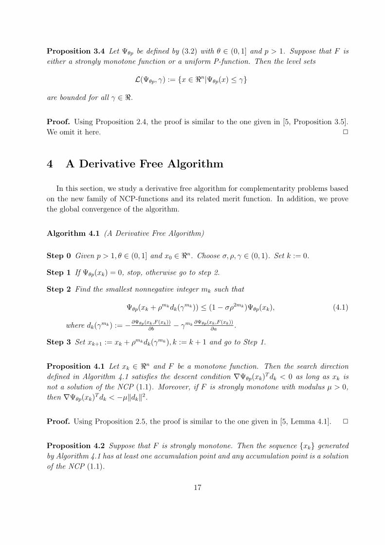
Proposition 3.4 Let Ψθp be defined by (3.2) with θ ∈ (0, 1] and p > 1. Suppose that F is

either a strongly monotone function or a uniform P-function. Then the level sets

L(Ψθp, γ) := {x ∈ <n|Ψθp(x) ≤ γ}

are bounded for all γ ∈ <.

Proof. Using Proposition 2.4, the proof is similar to the one given in [5, Proposition 3.5].

We omit it here. 2

4 A Derivative Free Algorithm

In this section, we study a derivative free algorithm for complementarity problems based

on the new family of NCP-functions and its related merit function. In addition, we prove

the global convergence of the algorithm.

Algorithm 4.1 (A Derivative Free Algorithm)

Step 0 Given p > 1, θ ∈ (0, 1] and x0 ∈ <n. Choose σ, ρ, γ ∈ (0, 1). Set k := 0.

Step 1 If Ψθp(xk) = 0, stop, otherwise go to step 2.

Step 2 Find the smallest nonnegative integer mk such that

Ψθp(xk + ρmkdk(γmk)) ≤ (1− σρ2mk)Ψθp(xk), (4.1)

where dk(γmk) := −∂Ψθp(xk,F (xk))

∂b− γmk

∂Ψθp(xk,F (xk))

∂a.

Step 3 Set xk+1 := xk + ρmkdk(γmk), k := k + 1 and go to Step 1.

Proposition 4.1 Let xk ∈ <n and F be a monotone function. Then the search direction

defined in Algorithm 4.1 satisfies the descent condition ∇Ψθp(xk)T dk < 0 as long as xk is

not a solution of the NCP (1.1). Moreover, if F is strongly monotone with modulus µ > 0,

then ∇Ψθp(xk)T dk < −µ‖dk‖2.

Proof. Using Proposition 2.5, the proof is similar to the one given in [5, Lemma 4.1]. 2

Proposition 4.2 Suppose that F is strongly monotone. Then the sequence {xk} generated

by Algorithm 4.1 has at least one accumulation point and any accumulation point is a solution

of the NCP (1.1).

17

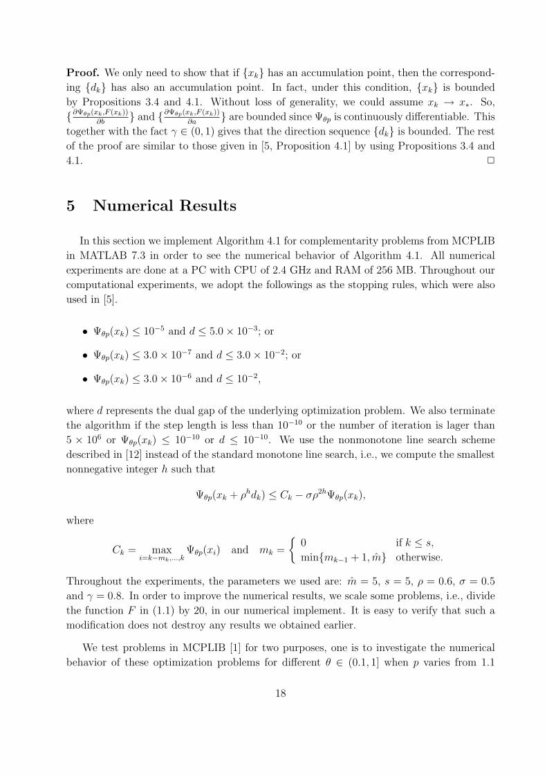
Proof. We only need to show that if {xk} has an accumulation point, then the correspond-

ing {dk} has also an accumulation point. In fact, under this condition, {xk} is bounded

by Propositions 3.4 and 4.1. Without loss of generality, we could assume xk → x∗. So,

{∂Ψθp(xk,F (xk))

∂b} and {∂Ψθp(xk,F (xk))

∂a} are bounded since Ψθp is continuously differentiable. This

together with the fact γ ∈ (0, 1) gives that the direction sequence {dk} is bounded. The rest

of the proof are similar to those given in [5, Proposition 4.1] by using Propositions 3.4 and

4.1. 2

5 Numerical Results

In this section we implement Algorithm 4.1 for complementarity problems from MCPLIB

in MATLAB 7.3 in order to see the numerical behavior of Algorithm 4.1. All numerical

experiments are done at a PC with CPU of 2.4 GHz and RAM of 256 MB. Throughout our

computational experiments, we adopt the followings as the stopping rules, which were also

used in [5].

• Ψθp(xk) ≤ 10−5 and d ≤ 5.0× 10−3; or

• Ψθp(xk) ≤ 3.0× 10−7 and d ≤ 3.0× 10−2; or

• Ψθp(xk) ≤ 3.0× 10−6 and d ≤ 10−2,

where d represents the dual gap of the underlying optimization problem. We also terminate

the algorithm if the step length is less than 10−10 or the number of iteration is lager than

5 × 106 or Ψθp(xk) ≤ 10−10 or d ≤ 10−10. We use the nonmonotone line search scheme

described in [12] instead of the standard monotone line search, i.e., we compute the smallest

nonnegative integer h such that

Ψθp(xk + ρhdk) ≤ Ck − σρ2hΨθp(xk),

where

Ck = maxi=k−mk,...,k

Ψθp(xi) and mk =

{0 if k ≤ s,

min{mk−1 + 1, m} otherwise.

Throughout the experiments, the parameters we used are: m = 5, s = 5, ρ = 0.6, σ = 0.5

and γ = 0.8. In order to improve the numerical results, we scale some problems, i.e., divide

the function F in (1.1) by 20, in our numerical implement. It is easy to verify that such a

modification does not destroy any results we obtained earlier.

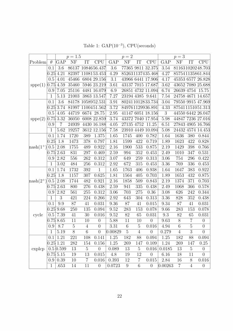
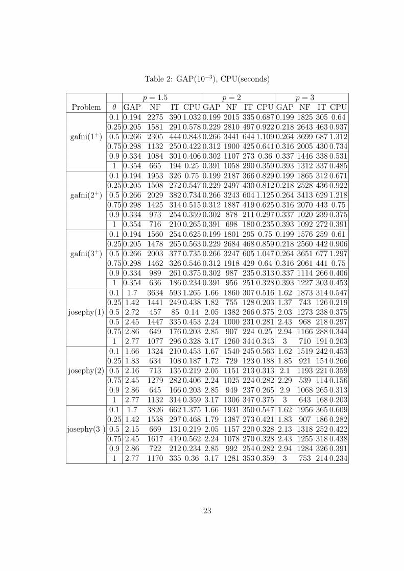
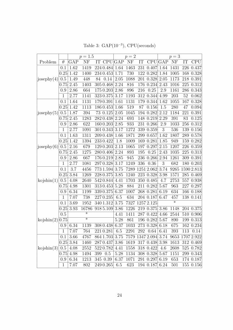
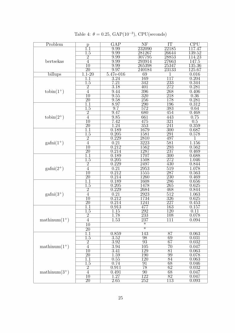
We test problems in MCPLIB [1] for two purposes, one is to investigate the numerical

behavior of these optimization problems for different θ ∈ (0.1, 1] when p varies from 1.1

18

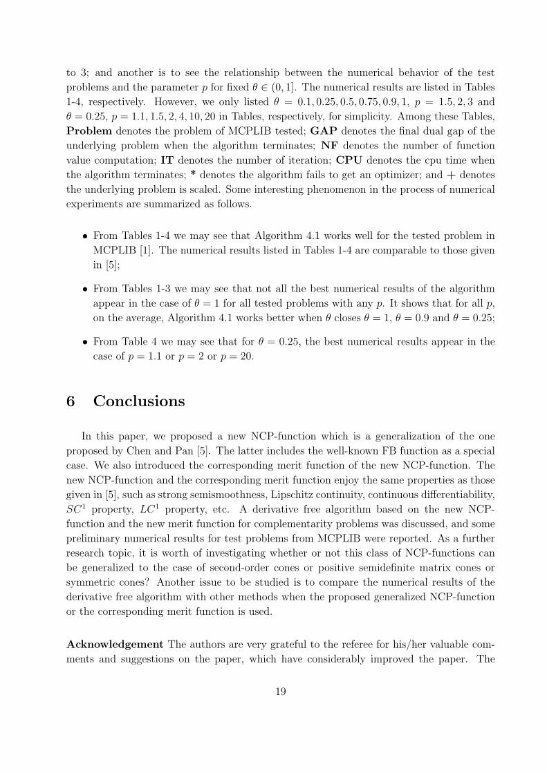
to 3; and another is to see the relationship between the numerical behavior of the test

problems and the parameter p for fixed θ ∈ (0, 1]. The numerical results are listed in Tables

1-4, respectively. However, we only listed θ = 0.1, 0.25, 0.5, 0.75, 0.9, 1, p = 1.5, 2, 3 and

θ = 0.25, p = 1.1, 1.5, 2, 4, 10, 20 in Tables, respectively, for simplicity. Among these Tables,

Problem denotes the problem of MCPLIB tested; GAP denotes the final dual gap of the

underlying problem when the algorithm terminates; NF denotes the number of function

value computation; IT denotes the number of iteration; CPU denotes the cpu time when

the algorithm terminates; * denotes the algorithm fails to get an optimizer; and + denotes

the underlying problem is scaled. Some interesting phenomenon in the process of numerical

experiments are summarized as follows.

• From Tables 1-4 we may see that Algorithm 4.1 works well for the tested problem in

MCPLIB [1]. The numerical results listed in Tables 1-4 are comparable to those given

in [5];

• From Tables 1-3 we may see that not all the best numerical results of the algorithm

appear in the case of θ = 1 for all tested problems with any p. It shows that for all p,

on the average, Algorithm 4.1 works better when θ closes θ = 1, θ = 0.9 and θ = 0.25;

• From Table 4 we may see that for θ = 0.25, the best numerical results appear in the

case of p = 1.1 or p = 2 or p = 20.

6 Conclusions

In this paper, we proposed a new NCP-function which is a generalization of the one

proposed by Chen and Pan [5]. The latter includes the well-known FB function as a special

case. We also introduced the corresponding merit function of the new NCP-function. The

new NCP-function and the corresponding merit function enjoy the same properties as those

given in [5], such as strong semismoothness, Lipschitz continuity, continuous differentiability,

SC1 property, LC1 property, etc. A derivative free algorithm based on the new NCP-

function and the new merit function for complementarity problems was discussed, and some

preliminary numerical results for test problems from MCPLIB were reported. As a further

research topic, it is worth of investigating whether or not this class of NCP-functions can

be generalized to the case of second-order cones or positive semidefinite matrix cones or

symmetric cones? Another issue to be studied is to compare the numerical results of the

derivative free algorithm with other methods when the proposed generalized NCP-function

or the corresponding merit function is used.

Acknowledgement The authors are very grateful to the referee for his/her valuable com-

ments and suggestions on the paper, which have considerably improved the paper. The

19

authors are also very grateful to Dr. Shaohua Pan (School of Mathematical Sciences, South

China University of Technology, P.R. China) for her help on implementing the algorithm

discussed in this paper.

References

[1] Billups S.C., Dirkse S.P., and Soares M.C., A comarison of algorithms for large scale

mixed complementarity problems, Comput. Optim. Appl., 7 (1977): 3–25.

[2] Chen B., Chen X., and Kanzow C., A penalized Fischer-Burmeister NCP-function. Math.

Program., 88 (2000): 211–216.

[3] Chen J.S., The semismooth-related properties of a merit function and a descent method

for the nonlinear complementarity problem. J. Global Optim., 36 (2006): 565–580.

[4] Chen J.S., On some NCP-function based on the generalized Fischer-Burmeister function.

Asia-Pac. J. Oper. Res., 24 (2007): 401–420.

[5] Chen J.S. and Pan S.H., A family of NCP functions and a desent method for the nonlinear

complementarity problem. Comput. Optim. Appl., 40 (2008): 389–404.

[6] Chen J.S. and Pan S.H., A regularization semismooth Newton method based on the gen-

eralized Fischer-Burmeister function for P0-NCPs. J. Comput. Appl. Math., 220 (2008):

464-479.

[7] Chen J.S. and Tseng P., An unconstrained smooth minimization reformulation of the

second-order cone complementarity problem. Math. Program., 104 (2005): 293–372.

[8] Clarke F.H., Optimization and Nonsmooth Analysis, Wiley, New York, 1983.

[9] Facchinei F. and Pang J.S., Finite-Dimensional Variational Inequalities and Complemen-

tarity Problems. Springer Verlag, New York, 2003.

[10] Ferris M.C. and Pang J.S., Engineering and economic applications of complementarity

problems. SIAM J. Rev., 39 (1997): 669–713.

[11] Fischer A., Solution of monotone complementarity problems with Lipschitzian func-

tions. Math. Program., 76 (1997): 513–532.

[12] Grippo L., Lampariello F., and Lucidi S., A nonmonotone line search technique for

Newton’s method. SIAM. J. Numer. Anal., 23 (1986): 707–716.

[13] Harker P.T. and Pang J.S., Finite dimensional variational inequality and nonlinear com-

plementarity problem: a survey of theory, algorithms and applications. Math. Program.,

48 (1990): 161–220.

20

[14] Huang Z.H., The global linear and local quadratic convergence of a non-interior con-

tinuation algorithm for the LCP. IMA J. Numer. Anal., 25 (2005): 670–684.

[15] Huang Z.H. and Gu W.Z., A smoothing-type algorithm for solving linear complemen-

tarity problems with strong convergence properties, Appl. Math. Optim., 57 (2008):

17–29.

[16] Huang Z.H., Qi L., and Sun D., Sub-quadratic convergence of a smoothing Newton

algorithm for the P0- and monotone LCP. Math. Program., 99 (2004): 423–441.

[17] Jiang H.Y., Fukushima M., Qi L. etal., A trust region method for solving generalized

complementarity problems. SIAM. J. Optim., 8 (1998): 140–157.

[18] Kanzow C. and Kleinmichel H., A new class of semismooth Newton method for nonlin-

ear complementarity problems. Comput. Optim. Appl., 11 (1998): 227–251.

[19] Kanzow C., Yamashita N., and Fukushima M., New NCP-functions and their properties.

J. Optim. Theory Appl., 94 (1997): 115–135.

[20] Mifflin R., Semismooth and semiconvex functions in constrained optimization. SIAM

J. Control Optim., 15 (1977): 957–972.

[21] Ortega J.M. and Rheinboldt W., Iterative Solution of Nonlinear Equations in Several

Variables. SIAM. Philadelphia. 2000.

[22] Pan, S.H. and Chen, J.S. A semismooth Newton method for the SOCCP based on

one-parametric class of SOC complementarity functions. To appear in Comput. Optim.

Appl., DOI: 10.1007/s10589-008-9166-9, 2008.

[23] Pang J.S., Complementarity problems. In: Horst, R., Pardalos, P. (eds.) Handbook

of Global Optimization. Kluwer Academic Publishers. Boston. Massachusetts. 1994, pp.

271–338.

[24] Qi L. and Sun J., A nonsmooth version of Newtons method. Math. Program., 58 (1993):

353–367.

[25] Sun D. and Qi L., On NCP-functions, Comput. Optim. Appl., 13 (1999) 201–220.

[26] Tseng P., Growth behaviour of a class of merit functions for the nonlinear complemen-

tarity problem. J. Optim. Theory Appl., 89 (1996): 17–37.

[27] Yamashita N. and Fukushima M., On stationary points of the implicit Lagrangian for

nonlinear complementarity problems. J. Optim. Theory Appl., 84 (1995): 653-663.

[28] Yamashita N. and Fukushima M., Modified Newton methods for solving a semismooth

reformulation of monotone complementarity problems. Math. Program., 76 (1997): 469-

491.

21

Table 1: GAP(10−3), CPU(seconds)

p = 1.5 p = 2 p = 3Problem θ GAP NF IT CPU GAP NF IT CPU GAP NF IT CPU

0.1 3.6 86137 1084656.437 3.6 77365 9811 32.375 3.54 811631020248.7030.25 4.21 82397 1108153.453 4.29 852631137435.468 4.27 857541135861.8440.5 4.01 45466 6804 29.156 3.1 43966 6441 17.906 4.17 45353 6577 26.828

sppe(1) 0.75 4.59 35460 5946 23.219 3.61 43137 7015 17.687 3.62 43652 7080 25.6880.9 7.05 25116 4481 16.079 6.9 26851 4732 11.094 6.74 26639 4754 15.751 5.13 21003 3863 13.547 7.27 23194 4385 9.641 7.54 24758 4671 14.657

0.1 3.6 84178 1058952.531 3.91 802411012833.734 3.04 79550 9915 47.9690.25 3.74 81997 1100451.562 3.72 849761129936.891 4.33 875411151051.3130.5 4.05 44719 6674 28.75 2.95 41147 6051 18.156 3 44550 6442 26.047

sppe(2) 0.75 3.32 36050 6008 22.859 3.74 43372 7040 17.954 5.98 44847 7236 27.0160.9 7 24939 4430 16.188 4.05 27135 4752 11.25 6.51 27843 4905 16.7661 5.62 19257 3612 12.156 7.58 23910 4449 10.094 5.08 24432 4574 14.453

0.1 1.74 1720 389 1.375 1.65 1745 400 0.782 1.64 1636 380 0.8440.25 1.8 1473 378 0.797 1.81 1599 422 0.719 1.89 1623 422 0.828

nash(1+) 0.5 2.08 1755 489 0.922 2.16 1900 533 0.875 2.19 1429 398 0.7660.75 2.63 831 297 0.469 2.59 994 352 0.453 2.49 1010 347 0.5310.9 2.82 556 262 0.312 3.07 649 259 0.313 3.06 754 296 0.4221 3.02 484 256 0.312 2.92 672 315 0.453 3.36 769 336 0.453

0.1 1.74 1732 392 1 1.65 1763 406 0.938 1.64 1647 383 0.9220.25 1.8 1157 307 0.625 1.81 1564 405 0.703 1.89 1653 432 0.875

nash(2+) 0.5 2.08 1744 482 0.921 2.16 1858 509 0.843 2.19 1374 371 0.7030.75 2.63 800 276 0.438 2.59 941 335 0.438 2.49 1068 366 0.5780.9 2.82 561 255 0.312 3.06 703 275 0.36 3.08 626 242 0.3441 3 421 224 0.266 2.92 643 304 0.313 3.36 828 352 0.438

0.1 9.9 87 41 0.031 9.36 87 41 0.015 9.34 87 41 0.0310.25 9.68 250 135 0.094 9.52 283 153 0.078 9.66 283 153 0.078

cycle 0.5 7.39 41 30 0.016 9.52 82 65 0.031 9.3 82 65 0.0310.75 8.65 11 10 0 5.88 11 10 0 9.63 8 7 00.9 8.7 5 4 0 3.31 6 5 0.016 4.94 6 5 01 5.19 8 6 0 0.00829 5 4 0 0.279 4 3 0

0.1 1.21 221 108 0.141 1.25 182 88 0.094 1.25 182 88 0.0940.25 1.21 282 154 0.156 1.25 269 147 0.109 1.24 269 147 0.25

explcp 0.5 0.599 13 5 0 0.089 13 5 0.016 0.0185 13 5 00.75 5.15 19 13 0.015 4.8 19 12 0 6.16 18 11 00.9 0.39 10 7 0.016 0.393 12 7 0.015 2.84 16 8 0.0161 .653 14 11 0 0.0723 9 6 0 0.00263 7 4 0

22

Table 2: GAP(10−3), CPU(seconds)

p = 1.5 p = 2 p = 3Problem θ GAP NF IT CPU GAP NF IT CPU GAP NF IT CPU

0.1 0.194 2275 390 1.032 0.199 2015 335 0.687 0.199 1825 305 0.640.25 0.205 1581 291 0.578 0.229 2810 497 0.922 0.218 2643 463 0.937

gafni(1+) 0.5 0.266 2305 444 0.843 0.266 3441 644 1.109 0.264 3699 687 1.3120.75 0.298 1132 250 0.422 0.312 1900 425 0.641 0.316 2005 430 0.7340.9 0.334 1084 301 0.406 0.302 1107 273 0.36 0.337 1446 338 0.5311 0.354 665 194 0.25 0.391 1058 290 0.359 0.393 1312 337 0.485

0.1 0.194 1953 326 0.75 0.199 2187 366 0.829 0.199 1865 312 0.6710.25 0.205 1508 272 0.547 0.229 2497 430 0.812 0.218 2528 436 0.922

gafni(2+) 0.5 0.266 2029 382 0.734 0.266 3243 604 1.125 0.264 3413 629 1.2180.75 0.298 1425 314 0.515 0.312 1887 419 0.625 0.316 2070 443 0.750.9 0.334 973 254 0.359 0.302 878 211 0.297 0.337 1020 239 0.3751 0.354 716 210 0.265 0.391 698 180 0.235 0.393 1092 272 0.391

0.1 0.194 1560 254 0.625 0.199 1801 295 0.75 0.199 1576 259 0.610.25 0.205 1478 265 0.563 0.229 2684 468 0.859 0.218 2560 442 0.906

gafni(3+) 0.5 0.266 2003 377 0.735 0.266 3247 605 1.047 0.264 3651 677 1.2970.75 0.298 1462 326 0.546 0.312 1918 429 0.64 0.316 2061 441 0.750.9 0.334 989 261 0.375 0.302 987 235 0.313 0.337 1114 266 0.4061 0.354 636 186 0.234 0.391 956 251 0.328 0.393 1227 303 0.453

0.1 1.7 3634 593 1.265 1.66 1860 307 0.516 1.62 1873 314 0.5470.25 1.42 1441 249 0.438 1.82 755 128 0.203 1.37 743 126 0.219

josephy(1) 0.5 2.72 457 85 0.14 2.05 1382 266 0.375 2.03 1273 238 0.3750.5 2.45 1447 335 0.453 2.24 1000 231 0.281 2.43 968 218 0.2970.75 2.86 649 176 0.203 2.85 907 224 0.25 2.94 1166 288 0.3441 2.77 1077 296 0.328 3.17 1260 344 0.343 3 710 191 0.203

0.1 1.66 1324 210 0.453 1.67 1540 245 0.563 1.62 1519 242 0.4530.25 1.83 634 108 0.187 1.72 729 123 0.188 1.85 921 154 0.266

josephy(2) 0.5 2.16 713 135 0.219 2.05 1151 213 0.313 2.1 1193 221 0.3590.75 2.45 1279 282 0.406 2.24 1025 224 0.282 2.29 539 114 0.1560.9 2.86 645 166 0.203 2.85 949 237 0.265 2.9 1068 265 0.3131 2.77 1132 314 0.359 3.17 1306 347 0.375 3 643 168 0.203

0.1 1.7 3826 662 1.375 1.66 1931 350 0.547 1.62 1956 365 0.6090.25 1.42 1538 297 0.468 1.79 1387 273 0.421 1.83 907 186 0.282

josephy(3 ) 0.5 2.15 669 131 0.219 2.05 1157 220 0.328 2.13 1318 252 0.4220.75 2.45 1617 419 0.562 2.24 1078 270 0.328 2.43 1255 318 0.4380.9 2.86 722 212 0.234 2.85 992 254 0.282 2.94 1284 326 0.3911 2.77 1170 335 0.36 3.17 1281 353 0.359 3 753 214 0.234

23

Table 3: GAP(10−3), CPU(seconds)

p = 1.5 p = 2 p = 3Problem θ GAP NF IT CPU GAP NF IT CPU GAP NF IT CPU

0.1 1.62 1419 224 0.484 1.64 1463 231 0.407 1.64 1431 226 0.4370.25 1.42 1400 234 0.453 1.71 730 122 0.282 1.84 1005 168 0.328

josephy(4) 0.5 1.49 448 84 0.14 2.05 1088 201 0.328 2.05 1173 218 0.3910.75 2.45 1403 305 0.468 2.24 816 176 0.234 2.43 1016 225 0.3120.9 2.86 664 175 0.203 2.86 896 216 0.25 2.9 1161 286 0.3431 2.77 1141 323 0.375 3.17 1193 312 0.344 4.99 203 52 0.062

0.1 1.64 1131 179 0.391 1.61 1131 179 0.344 1.62 1055 167 0.3280.25 1.42 1113 186 0.453 1.66 519 87 0.156 1.5 280 47 0.094

josephy(5) 0.5 1.87 394 73 0.125 2.05 1045 194 0.282 2.12 1184 221 0.3910.75 2.45 1283 282 0.438 2.24 693 148 0.219 2.29 391 83 0.1250.9 2.86 622 160 0.203 2.85 933 231 0.266 2.9 1033 256 0.3121 2.77 1091 301 0.343 3.17 1272 339 0.359 3 536 139 0.156

0.1 1.63 1311 209 0.438 1.66 1871 299 0.657 1.62 1807 289 0.5780.25 1.42 1394 233 0.422 1.8 1009 169 0.281 1.85 949 159 0.282

josephy(6) 0.5 2.16 679 129 0.203 2.13 1065 197 0.297 2.15 1207 226 0.3590.75 2.45 1275 280 0.406 2.24 893 195 0.25 2.43 1035 225 0.3130.9 2.86 667 176 0.219 2.85 945 236 0.266 2.94 1261 309 0.3911 2.77 1081 297 0.328 3.17 1249 336 0.36 3 682 180 0.203

0.1 3.7 4456 773 1.594 3.75 7289 1251 2.062 3.74 9265 1590 2.8130.25 3.84 1269 228 0.375 3.85 1240 223 0.328 3.98 1571 285 0.469

kojshin(1) 0.5 4.08 2640 542 0.844 4.41 1703 350 0.485 4.7 2753 557 0.9380.75 4.98 1301 313 0.453 5.28 884 211 0.282 5.67 963 227 0.2970.9 6.34 1199 339 0.375 6.37 1007 268 0.281 6.19 634 166 0.1881 7.07 738 227 0.235 6.5 634 204 0.187 6.47 457 138 0.141

0.1 3.69 1952 340 1.312 3.75 7327 1257 2.125 *0.25 3.93 16786 918 5.109 3.86 1226 219 0.375 3.86 1148 204 0.3750.5 * 4.41 1411 287 0.422 4.66 2544 510 0.906

kojshin(2) 0.75 * 5.28 861 196 0.282 5.67 890 199 0.3130.9 6.34 1139 308 0.438 6.37 1033 273 0.328 6.18 675 162 0.2341 7.07 764 221 0.281 6.5 2291 292 0.64 6.41 393 113 0.14

0.1 3.66 4767 864 1.703 3.75 7579 1347 2.094 3.74 9653 1707 2.9220.25 3.84 1460 287 0.437 3.86 1619 317 0.438 3.98 1613 312 0.469

kojshin(3) 0.5 4.08 2552 522 0.782 4.41 1558 318 0.422 4.6 2608 525 0.7820.75 4.98 1494 399 0.5 5.28 1134 308 0.328 5.67 1151 299 0.3430.9 6.34 1213 345 0.39 6.37 1071 291 0.297 6.19 653 174 0.1871 7.07 802 249 0.265 6.5 623 194 0.187 6.24 501 155 0.156

24

Table 4: θ = 0.25, GAP(10−3), CPU(seconds)

Problem p GAP NF IT CPU1.1 9.99 232090 22185 117.471.5 9.99 281267 26644 139.522 9.99 307795 28853 114.23

bertsekas 4 9.99 293914 27663 147.510 9.99 265398 25347 135.3620 9.97 240184 23133 125.67

billups 1.1-20 5.47e-016 69 1 0.0161.1 3.24 169 117 0.2041.5 7.21 342 233 0.3442 3.18 401 272 0.281

tobin(1+) 4 9.44 396 268 0.40610 9.55 320 218 0.3620 9.58 256 178 0.2811.1 8.97 290 196 0.3121.5 9.7 572 383 0.642 9.47 680 454 0.468

tobin(2+) 4 9.85 661 443 0.7510 7.42 475 321 0.520 1.24 353 241 0.3591.1 0.189 1679 300 0.6871.5 0.205 1581 291 0.5782 0.229 2810 497 1

gafni(1+) 4 0.21 3223 581 1.15610 0.212 1562 293 0.56220 0.214 1287 237 0.4691.1 0.189 1707 300 0.6881.5 0.205 1508 272 1.0462 0.229 2497 430 0.844

gafni(2+) 4 0.21 2953 519 1.07810 0.212 1555 287 0.56320 0.214 1260 230 0.4691.1 0.189 1608 286 0.6561.5 0.205 1478 265 0.6252 0.229 2684 468 0.844

gafni(3+) 4 0.21 2923 512 1.06310 0.212 1734 326 0.62520 0.214 1241 227 0.4531.1 0.913 477 163 0.1571.5 1.15 292 120 0.112 1.78 233 108 0.078

mathinum(1+) 4 1.53 237 111 0.09410 *20 *1.1 0.859 143 87 0.0631.5 3.52 98 69 0.0312 3.92 93 67 0.032

mathinum(1+) 4 3.94 105 70 0.04710 3.41 129 81 0.06320 1.59 190 99 0.0781.1 0.55 120 84 0.0631.5 0.74 91 68 0.0462 0.911 78 62 0.032

mathinum(3+) 4 0.491 90 68 0.04710 1.27 122 82 0.04720 2.65 252 113 0.093

25