Properties of Gauss digitized sets and digital surface ... · Properties of Gauss digitized sets...

Properties of Gauss digitized sets and digital surface

integration

Jacques-Olivier Lachaud, Boris Thibert

To cite this version:

Jacques-Olivier Lachaud, Boris Thibert. Properties of Gauss digitized sets and digital sur-face integration. [Research Report] Grenoble University; Universite de savoie. 2015. <hal-01070289v2>

HAL Id: hal-01070289

https://hal.archives-ouvertes.fr/hal-01070289v2

Submitted on 2 Oct 2015

HAL is a multi-disciplinary open accessarchive for the deposit and dissemination of sci-entific research documents, whether they are pub-lished or not. The documents may come fromteaching and research institutions in France orabroad, or from public or private research centers.

L’archive ouverte pluridisciplinaire HAL, estdestinee au depot et a la diffusion de documentsscientifiques de niveau recherche, publies ou non,emanant des etablissements d’enseignement et derecherche francais ou etrangers, des laboratoirespublics ou prives.

https://hal.archives-ouvertes.fr

https://hal.archives-ouvertes.fr/hal-01070289v2

PROPERTIES OF GAUSS DIGITIZED SHAPES AND DIGITAL SURFACE

INTEGRATION

JACQUES-OLIVIER LACHAUD AND BORIS THIBERT

October 2, 2015

Abstract. This paper presents new topological and geometric properties of Gauss digitizations ofEuclidean shapes, most of them holding in arbitrary dimension d. We focus on r-regular shapes sam-

pled by Gauss digitization at gridstep h. The digitized boundary is shown to be close to the Euclidean

boundary in the Hausdorff sense, the minimum distance√d2h being achieved by the projection map

ξ induced by the Euclidean distance. Although it is known that Gauss digitized boundaries may not

be manifold when d ≥ 3, we show that non-manifoldness may only occur in places where the normalvector is almost aligned with some digitization axis, and the limit angle decreases with h. We then

have a closer look at the projection of the digitized boundary onto the continuous boundary by ξ.

We show that the size of its non-injective part tends to zero with h. This leads us to study theclassical digital surface integration scheme, which allocates a measure to each surface element that

is proportional to the cosine of the angle between an estimated normal vector and the trivial surface

element normal vector. We show that digital integration is convergent whenever the normal estimatoris multigrid convergent, and we explicit the convergence speed. Since convergent estimators are now

available in the literature, digital integration provides a convergent measure for digitized objects.KeywordsGauss digitization and geometric inference and digital integral and multigrid convergence

and set with positive reach.

1. Introduction

Understanding what are the properties of real objects that can be extracted from their digitalrepresentation is a crucial task in knowledge representation and processing. In most applications, areal object or a scene is known only through some discrete finite representation, generally a digital imageproduced by some complex system, involving acquisition, sampling, quantization, and processing. Thisprocess is often called digitization or sampling and is realized by devices like CCD or CMOS cameras,document scanners, CT or MRI scanners. Since the digitization process aims to be as faithful aspossible to the real data, it is very natural to look at topological and geometric properties that canbe inferred from digital data for rather elementary digitization processes and classes of real Euclideanobjects.

This paper focuses on several global and local topological and geometric properties that are preservedby Gauss digitization.

Definition 1 (Gauss digitization). Let h > 0 be a sampling grid step. The Gauss digitization of anEuclidean shape X ⊂ Rd is defined as Dh(X) := X ∩ (hZ)d (see Fig. 1).

It is thus one of the simplest conceivable digitization scheme. We study here more specificallythe local connections between the boundary ∂X of the Euclidean shape and the boundary ∂hX ofits digitization (as an union of d − 1-dimensional cubic faces, see below). It is clear that one cannotexpect that many properties of real shapes be preserved by digitization for arbitrary digitization steph, just by some combinatorial argument. However one can expect that, as the grid step gets finer (hconverges to 0), we can recover most of the properties of the real shape from its digitization. Indeed,the literature shows that topological properties may be preserved for fine enough digitization grids

This work was partially supported by the ANR grants DigitalSnow ANR-11- BS02-009, KIDICO ANR-2010-BLAN-0205 and TopData ANR-13-BS01-0008.

This is an author version of the paper accepted in JMIV in 2015.

1

2 JACQUES-OLIVIER LACHAUD AND BORIS THIBERT

X ∂X DhX

h

QhDhX ∂hX

h

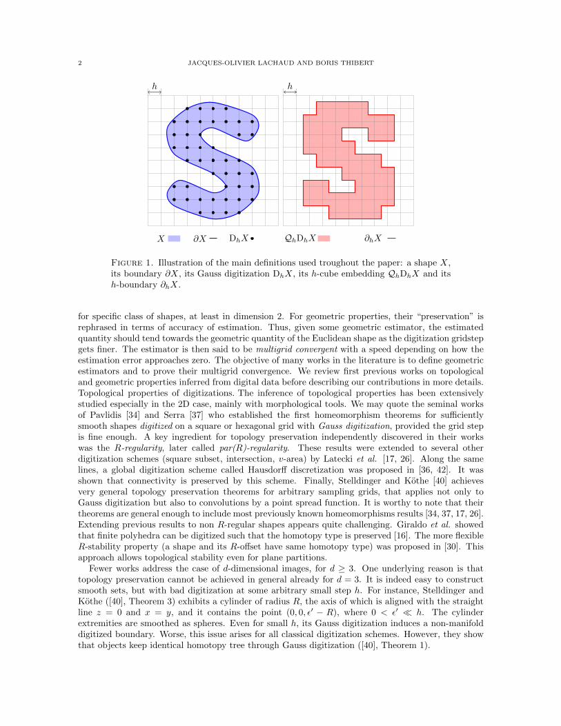
Figure 1. Illustration of the main definitions used troughout the paper: a shape X,its boundary ∂X, its Gauss digitization DhX, its h-cube embedding QhDhX and itsh-boundary ∂hX.

for specific class of shapes, at least in dimension 2. For geometric properties, their “preservation” isrephrased in terms of accuracy of estimation. Thus, given some geometric estimator, the estimatedquantity should tend towards the geometric quantity of the Euclidean shape as the digitization gridstepgets finer. The estimator is then said to be multigrid convergent with a speed depending on how theestimation error approaches zero. The objective of many works in the literature is to define geometricestimators and to prove their multigrid convergence. We review first previous works on topologicaland geometric properties inferred from digital data before describing our contributions in more details.Topological properties of digitizations. The inference of topological properties has been extensivelystudied especially in the 2D case, mainly with morphological tools. We may quote the seminal worksof Pavlidis [34] and Serra [37] who established the first homeomorphism theorems for sufficientlysmooth shapes digitized on a square or hexagonal grid with Gauss digitization, provided the grid stepis fine enough. A key ingredient for topology preservation independently discovered in their workswas the R-regularity, later called par(R)-regularity. These results were extended to several otherdigitization schemes (square subset, intersection, v-area) by Latecki et al. [17, 26]. Along the samelines, a global digitization scheme called Hausdorff discretization was proposed in [36, 42]. It wasshown that connectivity is preserved by this scheme. Finally, Stelldinger and Kothe [40] achievesvery general topology preservation theorems for arbitrary sampling grids, that applies not only toGauss digitization but also to convolutions by a point spread function. It is worthy to note that theirtheorems are general enough to include most previously known homeomorphisms results [34, 37, 17, 26].Extending previous results to non R-regular shapes appears quite challenging. Giraldo et al. showedthat finite polyhedra can be digitized such that the homotopy type is preserved [16]. The more flexibleR-stability property (a shape and its R-offset have same homotopy type) was proposed in [30]. Thisapproach allows topological stability even for plane partitions.

Fewer works address the case of d-dimensional images, for d ≥ 3. One underlying reason is thattopology preservation cannot be achieved in general already for d = 3. It is indeed easy to constructsmooth sets, but with bad digitization at some arbitrary small step h. For instance, Stelldinger andKothe ([40], Theorem 3) exhibits a cylinder of radius R, the axis of which is aligned with the straightline z = 0 and x = y, and it contains the point (0, 0, ε′ − R), where 0 < ε′ � h. The cylinderextremities are smoothed as spheres. Even for small h, its Gauss digitization induces a non-manifolddigitized boundary. Worse, this issue arises for all classical digitization schemes. However, they showthat objects keep identical homotopy tree through Gauss digitization ([40], Theorem 1).

PROPERTIES OF GAUSS DIGITIZED SHAPES AND DIGITAL SURFACE INTEGRATION 3

Several routes for solving the homeomorphism issue were proposed by Stelldinger et al. [41]. Afirst idea is to refine the digitized object on a twice finer grid by majority interpolation, and thisleads to a manifold digital surface close to the real object boundary (Theorem 19). They also proposeto recontruct from the digitized object an approximate surface based either on a union of ball, amodification of a marching-cubes algorithm, or a smoothing of the latter surface. Homeomorphism isachieved in all cases for fine enough grids.The projection map. Another path to handle topological or geometric inference problems is a morefunctional approach: the distance function to a shape and the associated projection map. It is a keytool since it encodes information on the shape and it is Hausdorff stable, whatever the dimension. Thedistance function of a compact set K is defined on Rd by dK(x) := min{‖x− y‖, y ∈ K}. The R-offsetof K, denoted by KR, is the set whose points x satisfy dK(x) ≤ R. The medial axis MA(K) of K isthe subset of Rd whose points have at least two closest points on K.

Definition 2 (Projection map). The projection map of a compact set K is the map

ξK : Rd \MA(K)→ K

that associates to any point x of Rd \MA(K) its unique closest point onto K.

The reach of K, denoted by reach(K), is the infimum of {dK(y), y ∈ MA(K)} [14]. The projectionmap ξK of a compact set K with positive reach is a useful tool because it allows to compare K withanother shape lying in its neighborhood.

Note that the R-offsets allow to recover stable topological (and geometric) properties. If the shapeK has positive reach and if a point cloud P is dense enough around K, then for some suitable valuesof R, the R-offsets of P are homotopy equivalent to K [5, 33]. This result has been extended fordigitizations close to K in the Hausdorff sense. They are shown to be homotopy equivalent to K, forsuitable values of digitization step size [1].Global geometric properties of digitizations. Infering geometric properties of Euclidean object fromtheir digitization has a long history. Until recently, most research efforts focused on global geometricproperties. For instance, The area (in 2D) or volume (in 3D) may indeed be estimated just by countingthe number of digital samples and this fact was known by Gauss and Dirichlet as reported for instancein [20]. Further results show that volumes and also moments may be estimated by appropriate countingwith even superlinear convergence for smooth enough classes of shapes [18, 22].

It is harder to define length/perimeter estimators in 2D or area estimators in 3D with provenconvergence. For length/perimeter, for specific classes of shapes, several approaches offer guaranteeslike segmentation into digital straight segments [22], ε-sausage approach [20], and minimum lengthpolygon [39]. A more local approach based on tangent estimation and integration leads also to multigrid

convergence with speed O(h13 ) [24, 23]. Few results exist for 3D area estimation. Most approaches

try to assign weights to local configurations in order to minimize the maximal error [28, 44], but suchapproaches cannot achieve multigrid convergence [19]. Polyhedrization with digital planes for areaestimation [21] is an interesting extension of 2D methods, but no theoretical guarantees have beenestablished.

Finally three methods offer (some) theoretical guarantees. Area estimation by integration of nor-mals, first proposed in [27] and more formalized in [6], has the advantage of defining an elementaryarea measure, which in turn can provide the global area measure but may also be used for integrationof other quantities. However their results rely on assumptions that are not satisfied by the Gaussdigitization boundary. A second approach estimates the volume of an appropriate thickened version ofthe surface, and deduced the area [41]. Their algorithm is not applicable as is on data since it requiresto loop over finer and finer digitizations of the continuous object. Besides it is in fact very similar toSteiner tube formula dating from 1840. A third approach relies on Cauchy-Crofton integral formulaand estimates area by statistical intersection of the volume with lines [29]. It it important to note thatall three methods do not provide an error bound. The speed of convergence of these estimators is thusunknown, even for specific classes of shapes.


Local geometric properties. It is often interesting to estimate more local geometric quantities likenormal vector or tangent planes, curvatures or principal directions. Since accuracy is ambiguous ata given sampling, the definition of multigrid convergence is adapted to local geometric quantities(e.g., see [9]). Several estimators are multigrid convergent: (i) digital straight segment recognitiondefines parameter-free convergent estimators of normal/tangent in 2D [11, 24, 23], (ii) polynomialfitting induces convergent estimators of derivatives of any order in 2D [35], (iii) binomial convolutionleads also to convergent estimators of derivatives in 2D [12, 13]; (iv) the recently introduced integralinvariants define multigrid convergent estimators of normals, 2D curvature, mean curvature [7], andalso 3D principal curvatures and principal directions [8].

Note that the distance function to a shape and its projection map also encode information on thenormals and on the curvatures. If K is a shape with positive µ-reach (a much less restrictive conditionthan positive reach), then the offset of point cloud approximating K provides estimation of the normals[2] and of the curvature measures [3, 4] of K at a given scale. Voronoi covariance measure [31] may alsobe adapted to digital data to define multigrid convergent normal estimators in arbitrary dimension[10].Contributions. We establish both topological preservation and multigrid convergence results. Afterrecalling useful notations and definitions in Section 2, Section 3 establishes elementary results onGauss digitized sets. We connect in Lemma 1 two notions: the R-regularity of shapes known indigital geometry [17, 26, 34, 37] and the reach of compact sets known in geometric measure theory [14]and computational geometry. Such shapes have a good behaviour with respect to digitization. Thenwe establish that ∂X and ∂hX are close to each other whatever the dimension (Theorem 1). Thisproximity is realized by the projection ξ of ∂hX onto ∂X induced by the Euclidean distance.

We then address the homeomorphism problem between these two sets, which is caused by thepossible non-manifoldness of the digitized boundary [40]. Although this problem is unavoidable startingfrom dimension 3, it is worth studying where non-manifoldness arises and if it is likely to arise often.With this information, it is then easier to take them into account, for instance to correct the digitaldataset [38]. In Section 4, we show local sufficient conditions which guarantee that the digitizedboundary is a manifold at this location (Theorem 2). They indicate that both sets ∂X and ∂hXare “almost” homeomorphic, and that the area of non-homeomorphic places reduces generally toward0 as the gridstep h gets finer and is reduced to 0. Furthermore, only places of ∂X with a normalvery close to some axis direction may induce a non-manifold place in ∂hX. This fact is illustratedon Fig. 2 as parts painted in dark grey on digitized boundary. Hence our approach is very differentfrom the one of Stelldinger et al. [41]. Instead of building a digitized surface different from the Gaussdigitized boundary to get a homeomorphism, we characterize the rare places where the Gauss digitizedboundary may not be a manifold.

Afterwards we establish in Section 5 several results related to the projection map between ∂Xand ∂hX. Even for smooth convex shapes, the projection map is not everywhere injective. HoweverTheorem 3 shows that the size of the non-injective part on ∂X decreases linearly in h. Fig. 2 shows inlight grey places where projection ξ might not be injective. Obviously, it includes zones in dark greywhere the digitized boundary is not even a manifold.

Finally, using results from geometric measure theory, Section 6 shows the conditions under whichdigital integration on ∂hX is multigrid convergent toward integration on ∂X, for an arbitrary inte-grable function from Rd to R. Given some digital normal estimator, digital integration is defined asproposed in [27, 6] by summation over digital d − 1-cells of the function value weighted by the innerproduct between trivial and estimated normal (see Definition 6). Theorem 4 demonstrates that digitalintegration is multigrid convergent toward usual integration as long as the normal estimator is multi-grid convergent. The convergence speed is also fully explicited and is upper bounded on the one handby the convergence speed of the normal estimator and on the other hand by the gridstep h. Sincemultigrid convergent normal estimators exist in arbitrary dimension [24, 8, 10], our theorem provesthat both local and global area estimation by digital integration is multigrid convergent, and it givesa well-defined measure on digitized boundary.


(a) h = 0.1 (b) h = 0.05 (c) h = 0.025Aξ = 58.40%, Anm = 1.57% Aξ = 30.71%, Anm = 0.38% Aξ = 15.88%, Anm = 0.09%

(a) h = 0.04 (b) h = 0.02 (c) h = 0.01Aξ = 62.22%, Anm = 0.88% Aξ = 30.54%, Anm = 0.12% Aξ = 16.67%, Anm = 0.03%

Figure 2. Illustration of Theorem 2 and Theorem 3 on several Gauss digitizationsof two polynomial surfaces (top row displays a Goursat’s smooth cube and bottomrow displays Goursat’s smooth icosahedron). Zones in dark grey indicates the surfaceparts where the Gauss digitization might be non manifold (Theorem 2); their relativearea is denoted by Anm. Zones in light grey (and dark grey) indicates the surfaceparts where projection ξ might not be an homeomorphism (Theorem 3); their relativearea is denoted by Aξ. Clearly, both zones tends to area zero as the gridstep gets finerand finer, while parts where digitization might not be manifold are much smaller thanparts where ξ might not be homeomorphic.

2. Preliminary notions and definitions

Given a compact shape X ⊂ Rd, we wish to compare the topological boundary of X, denoted by ∂X,with the boundary of its Gauss digitization. As defined in the introduction, the Gauss digitization ofX is a regular sampling of the characteristic function of X, with a parameterized sampling densityh. Digitized sets are defined as subsets of (hZ)d. Since they have peculiar coordinates (multiple ofh), points of such subsets will be called digital points. In order to define a digitized boundary, wehave to see the digitized set as a union of cubes with edge length h. For some z ∈ (hZ)d, the closedd-dimensional axis-aligned cube of Rd centered on z with edge length h is denoted by Qhz and calledh-cube. The h-cube embedding of a digital set Z is naturally defined as QhZ := ∪z∈ZQhz .


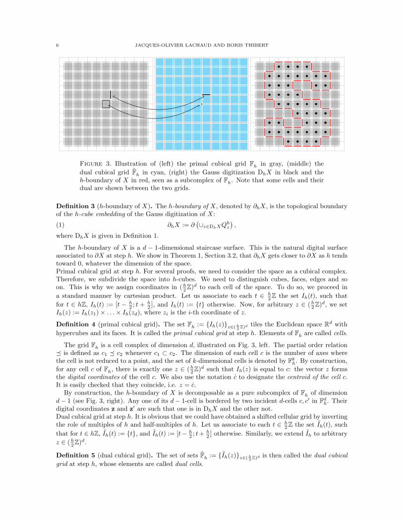
Figure 3. Illustration of (left) the primal cubical grid Fh in gray, (middle) the

dual cubical grid Fh in cyan, (right) the Gauss digitization DhX in black and theh-boundary of X in red, seen as a subcomplex of Fh. Note that some cells and theirdual are shown between the two grids.

Definition 3 (h-boundary of X). The h-boundary of X, denoted by ∂hX, is the topological boundaryof the h-cube embedding of the Gauss digitization of X:

(1) ∂hX := ∂(∪z∈DhXQ

hz

),

where DhX is given in Definition 1.

The h-boundary of X is a d − 1-dimensional staircase surface. This is the natural digital surfaceassociated to ∂X at step h. We show in Theorem 1, Section 3.2, that ∂hX gets closer to ∂X as h tendstoward 0, whatever the dimension of the space.Primal cubical grid at step h. For several proofs, we need to consider the space as a cubical complex.Therefore, we subdivide the space into h-cubes. We need to distinguish cubes, faces, edges and soon. This is why we assign coordinates in (h2Z)d to each cell of the space. To do so, we proceed in

a standard manner by cartesian product. Let us associate to each t ∈ h2Z the set Ih(t), such that

for t ∈ hZ, Ih(t) := [t − h2 ; t + h

2 ], and Ih(t) := {t} otherwise. Now, for arbitrary z ∈ (h2Z)d, we setIh(z) := Ih(z1)× . . .× Ih(zd), where zi is the i-th coordinate of z.

Definition 4 (primal cubical grid). The set Fh := {Ih(z)}z∈( h2 Z)d tiles the Euclidean space Rd with

hypercubes and its faces. It is called the primal cubical grid at step h. Elements of Fh are called cells.

The grid Fh is a cell complex of dimension d, illustrated on Fig. 3, left. The partial order relation� is defined as c1 � c2 whenever c1 ⊂ c2. The dimension of each cell c is the number of axes wherethe cell is not reduced to a point, and the set of k-dimensional cells is denoted by Fkh. By construction,

for any cell c of Fh, there is exactly one z ∈ (h2Z)d such that Ih(z) is equal to c: the vector z formsthe digital coordinates of the cell c. We also use the notation c to designate the centroid of the cell c.It is easily checked that they coincide, i.e. z = c.

By construction, the h-boundary of X is decomposable as a pure subcomplex of Fh of dimensiond− 1 (see Fig. 3, right). Any one of its d− 1-cell is bordered by two incident d-cells c, c′ in Fdh. Theirdigital coordinates z and z′ are such that one is in DhX and the other not.Dual cubical grid at step h. It is obvious that we could have obtained a shifted cellular grid by invertingthe role of multiples of h and half-multiples of h. Let us associate to each t ∈ h

2Z the set Ih(t), such

that for t ∈ hZ, Ih(t) := {t}, and Ih(t) := [t− h2 ; t+ h

2 ] otherwise. Similarly, we extend Ih to arbitrary

z ∈ (h2Z)d.

Definition 5 (dual cubical grid). The set of sets Fh := {Ih(z)}z∈( h2 Z)d is then called the dual cubical

grid at step h, whose elements are called dual cells.


It is clearly a cell complex, with the same definitions of partial order � and dimension. Digitalcoordinates and centroids are also defined similarly.

The sets Fkh and Fd−kh have a natural duality isomorphism induced between cells and dual cells withidentical coordinates. If we denote the duality operator on cells with the · operator, we clearly havefor c1, c2 ∈ Fh, c1 � c2 ⇔ c2 � c1. The dual cubical grid and its duality with the primal cubical gridare illustrated on Fig. 3, left and middle.Sets with positive reach and properties of projection map. The projection map ξ is continuous onRd \MA(K), and more precisely

Proposition 1 (Theorem 4.8 of [14]). Let K be a compact set with positive reach. Then for everyp ∈ K and every α ∈ [0, 1[, the projection ξK is 1

1−α Lipschitz in the ball centered on p with radius

α · reach(K).

In the particular case where K = ∂X is the boundary of a compact domain of Rd, we have thefollowing equivalence:

Proposition 2 ([14]). Let X be a compact domain of Rd. The reach of ∂X is strictly positive iff ∂Xis a hyper surface of class C1,1, which means that it is of class C1 and that the function that assignsthe normal to ∂X to each point x on ∂X is Lipschitz.

Remark that in Section 5 below, we will provide an explicit upper bound of the Lipschitz constantof the normal map (Lemma 5). Remark also that a manifold ∂X with strictly positive reach is thusof class C2 almost everywhere. This is a consequence of Rademacher Theorem (3.1.6 in [15]). In thefollowing, we will denote by ξ = ξ∂X the projection map on ∂X.R-regularity or par(R)-regularity. The R-regularity property was independently proposed by Pavlidis[34] and Serra [37]. Gross and Latecki introduced the similar definition of par(R)-regularity in [17],that is the shapes whose normal vectors do not intersect each other, when they are embedded assegments of length 2R. We prefer here to present the definition given in [26] with inside and outsideosculating balls. A closed ball iob(x,R) of radius R is an inside osculating ball of radius R to ∂X atpoint x ∈ ∂X if ∂X ∩ ∂iob(x,R) = {x} and iob(x,R) ⊆ X◦ ∪ {x}. A closed ball oob(x,R) of radiusR is an outside osculating ball of radius R to ∂X at point x ∈ ∂X if ∂X ∩ ∂oob(x,R) = {x} andoob(x,R) ⊆ (Rd \ X) ∪ {x}. A set X is then par(R,+)-regular if there exists an outside osculatingball of radius R at each x ∈ ∂X. A set X is par(R,−)-regular if there exists an inside osculating ballof radius R at each x ∈ ∂X. The par(R)-regularity is the conjunction of these two properties. Thisdefinition implies the other definition.

3. First properties of the boundary of Gauss digitized sets

In this section, we show that the notion of reach, which is classical in geometric measure theory,and the notion of par(R)-regularity, which is known in digital geometry, are related (Lemma 1). Wethen show that the boundary of X is close to its h-boundary in the Hausdorff sense, and we give tightbounds on the distance (Theorem 1) for arbitrary dimensions. Hence, digitized surfaces tends to theoriginal surface in the Hausdorff sense. Furthermore, the closest point is given by the projection map.

3.1. About R-regularity and positive reach. In the case where X is a d-dimensional object, thereach of ∂X and the R-regularity of X are related as follows.

Lemma 1. Let X be a d-dimensional compact domain of Rd. Then

reach(∂X) ≥ R ⇔ ∀R′ < R, X is par(R′)−regular.

Proof. Suppose that the reach of ∂X is strictly less than R. We want to show that there exists R′ < R,such that X is not par(R′)−regular. Since reach(∂X) < R, there exists a point x that has two closestpoints y1 and y2 on ∂X and such that d(x, ∂X) = R′′ < R. For simplicity, we assume that x ∈ X.(If x is outside X, then the proof is similar.) Let R′ be such that R′′ < R′ < R. We now proceedby contradiction: we assume that X is par(R′)−regular and we are going to show that there does not


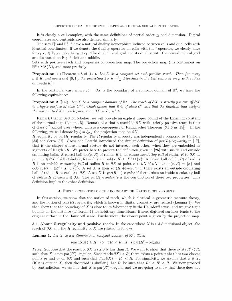
Figure 4. Illustration of the fact that the boundary of X and the h-boundary of X

are Hausdorff close, with distance no greater than√d

2 h. On the left, ∂hX lies in the√d

2 h-offset of ∂X (in gray). On the right, ∂X lies in the√d

2 h-offset of ∂hX (in gray).

exist any inside osculating ball to ∂X with center at x and radius R′, contradicting the hypothesisthat X is par(R′)−regular.

Note that the interior of the closed ball Bx(R′′) of center x and of radius R′′ = ‖x− y1‖ = ‖x− y2‖does not intersect ∂X, but Bx(R′′) intersects ∂X in at least the two points y1 and y2. Then, the ballBx(R′) of center x = y1 +R′ · (x− y1)/‖x− y1‖ and of radius R′ contains the point y2 in its interior,thus cannot be an inside osculating ball to ∂X at y1.

Consider now any other ball Bx(R′) of radius R′ whose center x does not belong to the straightline going through y1 and x and such that y1 ∈ ∂Bx(R′). We want to prove that Bx(R′) cannot bean inside osculating ball to ∂X at y1 either. Since X is assumed to be par(R′)-regular, there exists anoutside osculating ball Bx′(R

′) whose center x′ belongs to the straight line going through y1 and x, asthe two balls Bx(R′) and Bx′(R

′) are tangent at y1. But then the interior of the two balls Bx(R′) andBx′(R

′) must intersect, which implies that Bx(R′) does not belong entirely to the interior of X, sinceBx′(R

′) is an outside ball. So Bx(R′) cannot be an inside osculating ball to ∂X at y1. This contradictsthe fact that X is par(R′)-regular.

Let us show the reverse. We suppose that the reach of ∂X is larger than R and are going to showthat X is par(R′)-regular for every R′ < R. Since reach(∂X) ≥ R, we know that ∂X is a (d − 1)-manifold of class C1. Let y ∈ ∂X. There exists a unit normal ny to ∂X at y. Furthermore, for anyR′ < R, the point y+R′ ·ny is at a distance R′ from ∂X. Hence the ball By+R′·ny

(R′) only intersects∂X at the point y. Similarly, the ball By−R′·ny

(R′) also only intersects ∂X at the point y, whichimplies that X is par(R′)-regular. �

Remark 1. If X is a d-dimensional compact domain of Rd whose boundary ∂X has a reach greaterthan R, then for R′ < R, any point x ∈ ∂X has an inside osculating ball of radius R′ and an outsideosculating ball of radius R′.

3.2. Hausdorff distance between ∂X and its digital counterpart. We show in Theorem 1,below, that the boundary of X (in blue) and its digital counterpart ∂hX (in red) are close in theHausdorff sense, and this property is valid for arbitrary dimensions. This is illustrated on Fig. 4. Notethat a 2D version of this theorem was given in [23], Lemma B.9. For x ∈ ∂X, we denote by n(x, l) thesegment of length 2l, centered on x and aligned with the normal vector to ∂X at x.

Theorem 1. Let X be a compact domain of Rd such that the reach of ∂X is greater than R. Then,for any digitization step 0 < h < 2R/

√d, the Hausdorff distance between sets ∂X and ∂hX is less than


√dh/2. More precisely:

∀x ∈ ∂X,∃y ∈ ∂hX, ‖x− y‖ ≤√d

2 h and y ∈ n(x,√d

2 h),(2)

∀y ∈ ∂hX, ‖y − ξ(y)‖ ≤√d

2 h.(3)

Remark that this bound is tight.

Proof. We first prove (2). Let x ∈ ∂X. Since ∂X has reach greater than R, there is an inside osculating

ball of radius√d

2 h at x (from Remark 1 and h < 2R√d). There is also an outside osculating ball of same

radius at x. Let us denote by ci and ce their respective centers. Point ci (resp. ce) belongs to at least

one h-cube of center pi (resp. pe), i.e. some Qh. Since pi is at a distance less than or equal to√d

2 hfrom ci (half-diameter of h-cube), point pi belongs to the inside osculating ball at x and is thus a pointinside X◦ or is equal to x. Similarly point pe belongs to the complementary set of X or is equal to x.In the latter case, point ce is exactly in a corner of the h-cube Qhx and we choose for pe another h-cubecontaining ce, hence pe 6= x and pe ∈ Rd \X.

The straight segment [cice] is by definition the segment n(x,√d

2 h). We show by contradiction thatthis segment intersects ∂hX. Let D be the subset of h-cubes that intersect [cice]. We already knowthat D contains at least two h-cubes, one of center pi that is in X, one of center pe that is outsideX. By connectedness of segment [cice], there is a covering sequence (Pj)j=0..l of h-cubes included inD so that: (i) P0 has center pi, (ii) Pl has center pe, (iii) ∀j, with 0 ≤ j < l and Pj ∩ Pj+1 6= ∅. Sinceh-cubes are closed, it is easy to derive from (Pi) an enriched covering sequence (P ′j)j=0..l′ of sameextremeties such that any two consecutive h-cubes have a d− 1-dimensional intersection. Since P ′0 hascenter in X and P ′l′ has center outside X, there is an index k so that P ′k has center in X, and P ′k+1

has center outside X. By definition, P ′k ∩ P ′k+1 ⊂ ∂hX. Now, [cice] intersects both P ′k and P ′k+1 and,by convexity, their intersection. Let us denote by y this intersection. We have y ∈ P ′k ∩ P ′k+1 ⊂ ∂hX.

Since y ∈ [cice] = n(x,√d

2 h), y is at distance to x less than√d

2 h.We now prove (3). Let y ∈ ∂hX. By the definition of h-boundary (cf. (1)), there must exist two

h-cubes of center p1 and p2 such that p1 ∈ X and p2 6∈ X and they share a face (i.e. ‖p1 − p2‖1 = h).The closed straight segment [p1p2] thus intersects ∂X at least once, say at x′. By Pythagora’s theorem,

point x′ is at a distance less than√d

2 h from y. Since this distance is smaller than the reach of ∂X,

there is a unique point x onto ∂X that is closest to y. This implies that ‖y − x‖ ≤ ‖y − x′‖ ≤√d

2 h.

Furthermore, since ∂X is of class C1, the point y belongs to the line-segment normal to ∂X at x.

Putting these two facts together gives y ∈ n(x,√d

2 h). Clearly, this implies x = ξ(y) and (3). �

4. Manifoldness of the boundary of Gauss digitized sets

In the whole section, the set X is a compact domain of Rd, such that reach(∂X) is greater than somepositive constant R. Hence, X is par(R′)-regular for any 0 < R′ ≤ R (Lemma 1). Although Theorem 1states that the h-boundary of X tends to the boundary of X in the Hausdorff sense, starting fromd = 3 and as said in the introduction, the h-boundary of X may however not be a manifold. Focusingon d = 3, we thus exhibit local sufficient conditions which guarantee that the h-boundary is locally a2-manifold (see Theorem 2 below). These conditions indicates that only places of ∂X with a normalvery close to some axis direction may induce a non-manifold place in the h-boundary (dark grey zonesin Fig. 2). Even better, if the shape is not flat at these places, these zones tend to area zero with finerdigitization gridsteps.

Theorem 2 (Manifoldness sufficient condition). Let X be some compact domain of R3, with reach(∂X)greater than some positive constant R and h < 0.198R. Let y be a point of ∂hX.

i) If y does not belong to some 1-cell of ∂hX that intersect ∂X, then ∂hX is homeomorphic to a2-disk around y.

ii) If y belongs to some 1-cell s of ∂hX such that ∂X ∩ s contains a point P and if the angle αybetween s and the normal to ∂X at P satisfies αy ≥ 1.260h/R, then ∂hX is homeomorphic toa 2-disk around y.


The proof relies on the determination of necessary conditions for the presence of crossed configu-rations in the digitized set Dh(X). A digital set without crossed configuration has the property tobe well-composed [25]. And a well-composed set has a boundary that is a 2-manifold. The followingsubsections detail the steps of the proof of Theorem 2.

4.1. Terminology. Let 1X be the indicator function of X. Hence, for any z ∈ (hZ)3, z ∈ Dh(X) ⇔1X(z) = 1. Any dual 3-cell v of F3

h is a cube of side h and whose eight vertices (vi)0≤i≤7 arepoints of (hZ)3, numbered according to the lexicographic ordering of their z, y, x coordinates. The 8-configuration of X at v is the 8-tuple 1X(v) := (1X(v0), . . . , 1X(v7)). Let s be a dual 2-cell that is a faceof v. It is a square of side h whose four vertices s0, s1, s2, s3 are points of (hZ)3, numbered counterclock-wise when standing at the tip of the 1-cell s with maximal coordinate and looking at s. They form a sub-set of (vi)0≤i≤7. The 4-configuration of X at s is the 4-tuple 1X(s) := (1X(s0), 1X(s1), 1X(s2), 1X(s3)).

A crossed 8-configuration is any rotation or complementation of (1, 0, 0, 0, 0, 0, 0, 1) (there are 8 suchconfigurations). A crossed 8-configuration at a dual 3-cell v induces a non-manifold vertex in the h-boundary of X, precisely at the primal 0-cell v. It corresponds locally to two cubes glued together onlyat one vertex. A crossed 4-configuration is either the 4-configuration (1, 0, 1, 0) or the 4-configuration(0, 1, 0, 1). It is obvious that a crossed 4-configuration at a dual 2-cell s induce a non-manifold edgein the h-boundary of X, precisely at the primal 1-cell s. It corresponds locally to two cubes gluedtogether only along one edge. We recall (and adapt with our notations) Proposition 2.1 of [25].

Proposition 3 ([25]). The h-boundary of X is a 2-dimensional manifold if and only if X has no

crossed configurations in any dual 2-cell or 3-cell of Fh. (In this case, DhX is called a well-composedpicture.)

Non-manifoldness is thus determined by the presence of crossed configurations. We will thus exhibitsufficient conditions that prevent them to appear.

4.2. Relations between crossed configurations and grid step. We study the presence of crossedconfigurations depending on whether the boundary ∂X intersects or not cells of the cubical grid sampledat step h. The first lemma is straightforward.

Lemma 2. If ∂X does not intersect a dual 2-cell s of F2h, then the 4-configuration of X at s is not

crossed.

Proof. Then s ⊂ R3 \ ∂X = X◦ ∪ (R3 \X). Since s is connected while the previous union is disjoint,we have two cases, either s ⊂ X◦ and the 4-configuration is (1, 1, 1, 1), or s ⊂ R3 \ X and the 4-configuration is (0, 0, 0, 0). �

The second case tackled below is more involved. The idea is to look at how inner or outer osculatingballs contains vertices of s or s. It appears that crossed 4-configurations cannot arise when h is smallenough.

Lemma 3. Let h ≤ 0.198R. If ∂X intersects a dual 2-cell s of F2h but does not intersect the corre-

sponding primal 1-cell s, then the 4-configuration of X at s is not crossed.

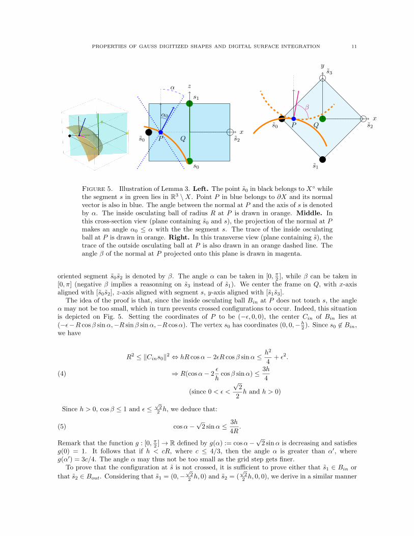
Proof. This lemma is illustrated on Fig. 5. If all vertices of s are in X, or all vertices of s are outsideX, then the 4-configuration of X at s is clearly not crossed and we are done. Hence at least one vertexof s, say s0, is in X (but may be on ∂X) and at least one other vertex of s is outside X. We assumehere that the primal 1-cell s (a segment of length h whose extremities are denoted by s0 and s1) liesoutside X. Should the 1-cell s be completely inside X◦, then we would reason on the vertex of sthat lies outside X, and the reasonning would be symetrical. Without loss of generality, let s0 be thisvertex in X, and let Q be the center of s0s2. The segment [s0Q] is a connected set that joins a pointin X to a point in R3 \X (since Q ∈ s). Hence, there exists a point P ∈ [s0Q] ∩ ∂X. According toRemark 1, there is thus an inside osculating ball Bin and an outside osculating ball Bout of radius Rat P . Let α be the angle between the normal n to ∂X at P and the segment s (oriented in the same

direction). Let n be the projection of n onto the plane Π supporting s. The angle between n and the


QPs0 s2

s0

s1

x

z

α0

α

QPs0

s1

s2

s3

x

y

β

Figure 5. Illustration of Lemma 3. Left. The point s0 in black belongs to X◦ whilethe segment s in green lies in R3 \X. Point P in blue belongs to ∂X and its normalvector is also in blue. The angle between the normal at P and the axis of s is denotedby α. The inside osculating ball of radius R at P is drawn in orange. Middle. Inthis cross-section view (plane containing s0 and s), the projection of the normal at Pmakes an angle α0 ≤ α with the the segment s. The trace of the inside osculatingball at P is drawn in orange. Right. In this transverse view (plane containing s), thetrace of the outside osculating ball at P is also drawn in an orange dashed line. Theangle β of the normal at P projected onto this plane is drawn in magenta.

oriented segment s0s2 is denoted by β. The angle α can be taken in [0, π2 ], while β can be taken in[0, π] (negative β implies a reasonning on s3 instead of s1). We center the frame on Q, with x-axisaligned with [s0s2], z-axis aligned with segment s, y-axis aligned with [s1s3].

The idea of the proof is that, since the inside osculating ball Bin at P does not touch s, the angleα may not be too small, which in turn prevents crossed configurations to occur. Indeed, this situationis depicted on Fig. 5. Setting the coordinates of P to be (−ε, 0, 0), the center Cin of Bin lies at(−ε−R cosβ sinα,−R sinβ sinα,−R cosα). The vertex s0 has coordinates (0, 0,−h2 ). Since s0 6∈ Bin,we have

R2 ≤ ‖Cins0‖2 ⇔ hR cosα− 2εR cosβ sinα ≤ h2

4+ ε2.

⇒ R(cosα− 2ε

hcosβ sinα) ≤ 3h

4(4)

(since 0 < ε <

√2

2h and h > 0)

Since h > 0, cosβ ≤ 1 and ε ≤√

22 h, we deduce that:

cosα−√

2 sinα ≤ 3h

4R.(5)

Remark that the function g : [0, π2 ]→ R defined by g(α) := cosα−√

2 sinα is decreasing and satisfiesg(0) = 1. It follows that if h < cR, where c ≤ 4/3, then the angle α is greater than α′, whereg(α′) = 3c/4. The angle α may thus not be too small as the grid step gets finer.

To prove that the configuration at s is not crossed, it is sufficient to prove either that s1 ∈ Bin or

that s2 ∈ Bout. Considering that s1 = (0,−√

22 h, 0) and s2 = (

√2

2 h, 0, 0), we derive in a similar manner


the following relations:

s1 ∈ Bin ⇔ ‖Cins1‖2 < R2

⇐ h

R sinα< (√

2 sinβ − 2ε

hcosβ)

⇐ h

R sinα<√

2 sinβ −√

2 cosβ,(6)

since ε < h/√

2, and

s2 ∈ Bout ⇔ ‖Couts2‖2 < R2

⇐ h

R sinα< (

√2

2cosβ +

ε

hcosβ)

⇐ h

R sinα<

√2

2cosβ,(7)

since 0 ≤ ε. It is thus enough for h/(R sinα) to be lower than the maximum of both bounds

a(β) :=√

2 sinβ−√

2 cosβ and b(β) :=√

22 cosβ of (6) and (7). One can show that there is a unique

value β′ ∈ [0, π] such that a(β′) = b(β′). This value is given by β′ = tan−1(3/2). It is easily seen that

for every β ∈ [0, π], one has a(β′) = b(β′) ≤ max(a(β), b(β)). Since a(β′) =√

2613 , it follows

h

R sinα<

√26

13=⇒ s1 ∈ Bin or s2 ∈ Bout.(8)

We now wish to find the best constant c such that, when h < cR, either s1 ∈ Bin or s2 ∈ Bout, and thus

the configuration is not crossed. We choose c such that 43c = g(α′) and α′ is given by c

sinα′ =√

2613 .

In that case, it follows from (5) that g(α) ≤ g(α′). Since g is decreasing, one has α ≥ α′, and thusc

sinα ≤c

sinα′ =√

2613 . This implies by (8) that either s1 ∈ Bin or s2 ∈ Bout. A simple computation

gives

tanα′ =52

3√

26 + 52√

2.

which implies that

c =4√

26√2704 + (52

√2 + 3

√26)2

Numerical approximation gives c ≈ 0.198. �

We turn ourselves to the last case, where we show that the direction of the normal to ∂X plays arole in the manifoldness of its digitized counterpart.

Lemma 4. Assume ∂X intersects a primal 1-cell s of F1h at some point P . Let α be the angle between

the normal n at P and the vector u aligned with direction s. Then the 4-configuration of X at s is notcrossed whenever 1.260 hR < α.

Proof. The idea is to measure the distance between vertices si (for i ∈ {0, 1, 2, 3}) and the center ofthe inside (resp. outside) osculating ball at P . Such osculating balls of radius R exist according toRemark 1. If this distance is smaller than R then we know that the value of 1X(si) is 1 (resp. 0).Indices i are taken modulo 4. The distance of P to s is denoted by ε. Without loss of generality,the angle α is taken in [0, π2 ]. Otherwise, a symmetric reasonning can be applied with the outsideosculating ball. The frame denoted Πi is centered on P with x-axis directed as [sisi+2] and with z-axisdirected as s, and oriented such that si has non positive z-coordinate. As in the proof of the previouslemma, let n be the projection of the outer normal at P onto the plane Π supporting s. The anglebetween n and the oriented segment [sisi+2] is denoted by βi.


Since α and βi represents the latitude and longitude of vector n, the center Cin of the insideosculating ball has coordinates −R (sinα cosβi, sinα sinβi, cosα) in frame Πi. Furthermore, point sihas coordinates (−

√2

2 h, 0,−ε). Since the inside osculating ball is in X◦, we deduce

1X(si) = 1⇐ ‖Cinsi‖2 < R2

⇔ h2

2+ ε2 <

√2Rh sinα cosβi + 2εR cosα

⇐ 3

4

h

R<√

2 sinα cosβi + 2ε

hcosα,(9)

since ε ≤ h2 . When angle βi ∈ [−π4 ,

π4 ], we have cosβi ≥

√2

2 . Inserting also ε ≥ 0 into (9) gives

1X(si) = 1⇐ 3

4

h

R< sinα

⇐ 1.179h

R< α,(10)

using απ/2 ≤ sinα and 3π

8 ≈ 1.1781.

Clearly there is at least one βj ∈ [−π4 ,π4 ]. Hence 1X(sj) = 1 for 1.179 hR < α. We prove either that

the opposite vertex to sj on s is outside X, i.e. 1X(sj+2) = 0, or that one of the neighboring vertex ofsj is inside X, i.e. 1X(sj+1) = 1 or 1X(sj−1) = 1. We prove the case βj ∈ [0, π4 ], hence we determinethe bounds for which either 1X(sj+2) = 0 or 1X(sj+1) = 1. Negative values of βj are tackled similarlywith 1X(sj−1) = 1.

One easily checks that, in the frame Πj , sj+1 = (0,−√

22 h,−ε), sj+2 = (

√2

2 h, 0,−ε) and the cen-ter Cout of the outside osculating ball has symmetric coordinates to Cin, i.e. Cout = −Cin. Withcomputations similar to (10), we derive

1X(sj+2) = 0⇐ ‖Coutsj+2‖2 < R2

⇐ 3

4

h

R<√

2 sinα cosβj − 2ε

hcosα.(11)

1X(sj+1) = 1⇐ ‖Cinsj+1‖2 < R2

⇐ 3

4

h

R<√

2 sinα sinβj + 2ε

hcosα.(12)

It is sufficient to have either (11) or (12) to get a non crossed configuration. We look therefore at the

maximum of both values. Denoting f(α, ν) :=√

2 sinα cosβj−2ν cosα and g(α, ν) :=√

2 sinα sinβj+2ν cosα, we rewrite those equations as:

1X(sj+2) = 0 or 1X(sj+1) = 1⇐ 3

4

h

R< max

(f(α,ε

h

), g(α,ε

h

))⇐ 3

4

h

R<

√2

2

√f2(α,ε

h

)+ g2

(α,ε

h

).(13)

The last implication comes from the property that√a2 + b2/

√2 ≤ max(a, b) holds not only for

positive values a and b but in the more general case where −min(a, b) ≤ max(a, b). Here f may takenegative values but, when negative, it is always smaller in absolute value than g. Simple calculationsgive:

f2(α, ν) + g2(α, ν) = 8 cos2 αν2 − 2√

2 sinα cosα(cosβj − sinβj)ν + 2 sin2 α

≥ 8 cos2 αν2 − 2√

2 sinα cosαν + 2 sin2 α,(14)


since βj ∈ [0, π4 ]. The last term is a degree 2 polynomial in ν that we denote hα(ν). It has discriminant

−56 sin2 α cos2 α, which is non positive for arbitrary α ≥ 0. Hence, hα(ν) takes minimum value at

να =√

28 tanα. Simple calculations lead to

f2(α, ν) + g2(α, ν) > hα(να) =7

4sin2 α >

7

π2α2,(15)

since sinα ≥ α/(π/2). Inserting inequality (15) into (13) implies:

1X(sj+2) = 0 or 1X(sj+1) = 1⇐ 3

4

h

R<

√2

2

√7

πα

⇐ 1.260h

R< α,(16)

since 3√

14π28 ≈ 1.2594. If both (10) and (16) hold, then the configuration at s is one of (1, 1, ?, ?),

(1, ?, 0, ?) and circular permutations. Hence the configuration is not crossed when 1.260 hR < α. �

To get an idea of the practical implication of previous Lemma, if one consider a shape with reach1, then there might be a non-manifold zone on its digitization at gridstep 1

10 only at places where thenormal makes an angle smaller than 7.5◦ with one axis. For instance, this is less than 2.57% of thearea on a sphere. We have now all the pieces to finish the proof of Theorem 2.

of Theorem 2. According to Proposition 3, the manifoldness of ∂hX is determined by the absence ofcrossed configurations. Non manifoldness at a primal vertex v occurs only if the 8-configuration of Xat v is crossed. Theorem 13 of [41] together with the equivalence of par-regularity and reach given byLemma 1 show that h < 0.5R implies that the the 8-configuration is not crossed. Non manifoldnessat a primal edge s occurs only if the 4-configuration of X at s is crossed. This case is fully studied inLemma 2, Lemma 3 and Lemma 4. Non manifoldness at a primal 2-cell is impossible by construction.This concludes the proof. �

5. Size of the non injective part

Here, the set X is a compact domain of Rd, whose boundary ∂X has reach strictly greater than R.We assume that h ≤ R/

√d, which implies by Theorem 1 that the Hausdorff distance between ∂X and

∂hX is less than R/2. Therefore the projection map ξ on ∂X is well defined on ∂hX. However, thismap is not one-to-one in general.

The aim of this section is to show that the subset of ∂X for which ξ is not injective from ∂hX,otherwise said the part of ∂X with multiplicity greater than one through projection, is small. Wedefine the following set

mult(∂X) := {x ∈ ∂X, s.t. ∃y1, y2 ∈ ∂hX, y1 6= y2 and ξ(y1) = ξ(y2) = x}.

Theorem 3. If h ≤ R/√d, then one has

Area (mult(∂X)) ≤ K1(h) Area (∂X) h,

where

K1(h) =4√

3 d2

R+O(h) ≤ 2

√3 d2 4d

R.

Here and in the sequel, the constant appearing in O(h) only involves the dimension d and the reachR. Furthermore, the (d− 1)-dimensional Hausdorff measure is denoted by Area and the d-dimensionalHausdorff measure is denoted by Vol.


5.1. Sketch of proof. The assumption h ≤ R/√d implies by Theorem 1 that the Hausdorff distance

between ∂hX and ∂X is less than√dh/2. In particular, one has for every y ∈ ∂hX, ‖y−ξ(y)‖ ≤

√dh/2.

Furthermore, Theorem 1 also implies that the restriction of the projection map to ∂hX is surjective.However, it may not be injective in general. We introduce the set mult(∂hX) = ξ−1(mult(∂X)).Clearly, the map

ξ : ∂hX \mult(∂hX)→ ∂X \mult(∂X)

is one-to-one. For any point x ∈ ∂X, we denote by n(x) the outward unit normal vector to ∂X atx and by nh(y) the outward unit normal vector to ∂hX at y. Remark that nh(y) is defined almosteverywhere for the (d− 1) Hausdorff measure. If y belongs to the intersection of two or more (d− 1)-dual cells, then we can choose for nh(y) the outward unit normal to any of those cells. The outline ofthe proof is the following:

i) We show that the scalar products between normals of ∂hX and ∂X is always greater than

−2√dh/R.

ii) We show that mult(∂X) ⊂ ξ(P (h)), where

P (h) := {y ∈ ∂hX, n(ξ(y)) · nh(y) ≤ 0}.

iii) We show that the jacobian of ξ at y is approximately |n(ξ(y)) · nh(y)|, hence the jacobian ofits restriction to P (h) is in O(h).

iv) We conclude that Area (mult(∂X)) is in O(h).

5.2. Angle relation between object boundary and its digitization. Let X be a compact domainof Rd, whose boundary ∂X has reach strictly greater than R. By Proposition 2, we know that ∂X isof class C1,1, meaning that the normal to ∂X is Lipschitz. We provide below an explicit upper boundof this Lipschitz constant.

Lemma 5. For any x1, x2 ∈ ∂X, one has

(17) ‖n(x1)− n(x2)‖ ≤√

3

R‖x1 − x2‖.

Proof. For i = 1, 2 we denote by ci the center of the outside osculating ball of radius R to ∂X at thepoint xi, by c′i the center of the inside osculating ball to ∂X at the point xi. Since the ball Bc1(R) isincluded in X and Bc′2(R) is included in the closure of Rd \X, their interior do not intersect and thus‖c1 − c′2‖ ≥ 2R. From the fact that ci − xi = R n(xi), one has

c1 − c′2 = (c1 − x1) + (x1 − x2) + (x2 − c′2)

= R n(x1) + (x1 − x2) +R n(x2),

which implies that

‖c1 − c′2‖2 = 2R2 + ‖x1 − x2‖2 + 2R2 n(x1) · n(x2)

+ 2R(x1 − x2) · [n(x1) + n(x2)] .

The condition ‖c1 − c′2‖2 ≥ 4R2 thus implies that

R2‖n(x1)− n(x2)‖2 = 2R2 [1− n(x1) · n(x2)]

≤ ‖x1 − x2‖2 + 2R (x1 − x2) · [n(x1) + n(x2)] .(18)

It remains to show that 2R (x1 − x2) · [n(x1) + n(x2)] is bounded by 2‖x1 − x2‖2, which will allowto conclude. Remark that the two points x1 and x1 + 2Rn(x1) belong to the sphere ∂Bc1(R) and arediametrally opposed. Thus, since x2 does not belong to the ball Bc1(R), one has

(x2 − x1) · (x2 − (x1 + 2R n(x1))) ≥ 0

⇔ (x2 − x1) · ((x2 − x1)− 2R n(x1)) ≥ 0

⇔ 2R (x2 − x1) · n(x1) ≤ ‖x2 − x1‖2


Similarly, since x2 does not belong to the ball Bc′1(R), the same inequality holds by replacing n(x1)with −n(x1) and thus

|2R (x2 − x1) · n(x1)| ≤ ‖x2 − x1‖2.Similarly, x1 does not belong to Bc2(R) ∪Bc′2(R), which implies

|2R (x2 − x1) · n(x2)| ≤ ‖x2 − x1‖2.Plugging these last two equations into (18) leads to

R2 ‖n(x1)− n(x2)‖2 ≤ 3 ‖x2 − x1‖2,which allows to conclude. �

Lemma 6. Let p ∈ X and q 6∈ X, then there exists x ∈ ∂X ∩ [pq] such that n(x) · −→pq ≥ 0.

Proof. First of all, X ∩ [pq] is not empty (it contains at least p) and is compact. In this compact set,we define x as the closest point to q. It is also clear that x ∈ ∂X. Assume that n(x) · −→pq < 0, then theinside osculating ball at x of radius R intersect of (xq]. This is a contradiction since x was the closestpoint of X to q along this segment. �

Lemma 7. For any y ∈ ∂hX, the angle between the normal nh(y) of any (d-1)-cell of ∂hX containingy and the normal of its projection x = ξ(y) onto ∂X satisfies:

n(x) · nh(y) ≥ −√

3d

Rh.

Proof. Let x = ξ(y). If n(x)·nh(y) is positive, the result is obvious. We suppose now that n(x)·nh(y) <0. Since y ∈ ∂hX, it belongs to a primal 2-cell c, whose dual 1-cell c is a segment [pq], where p ∈ X andq 6∈ X. Note that the normal nh(y) at y on ∂hX points in the same direction as the vector −→pq. Then weapply Lemma 6 for segment [pq], and we denote by x2 the point of ∂X∩[pq] such that n(x2)·nh(y) ≥ 0.

By Theorem 1, equation (3), we have that ‖x− y‖ ≤√d

2 h. Since y ∈ c and x2 ∈ [pq] = c, we also have

‖y− x2‖ ≤√d

2 h. We conclude by the triangle inequality that ‖x− x2‖ ≤√dh. Since h < R√

d, one has

‖x− x2‖ ≤ R, and one can apply Lemma 5

|n(x) · nh(y)| ≤ |(n(x)− n(x2)) · nh(y)|

≤ ‖n(x)− n(x2)‖ ≤√

3

R

√dh.

�

5.3. Parameterization of mult(∂X).

Lemma 8. For every x ∈ mult(∂X), there exists y ∈ ∂hX and a 2-cell c containing y, such that

ξ(y) = x and n(x) · nh(c) ≤ 0.

Proof. Let x ∈ mult(∂X) and [ab] = n(x,√dh/2) the segment centered in x of length

√dh and aligned

with the normal n(x). We suppose that this segment touches several (d− 1)-faces of ∂hX and is notin the tangent plane of one of these faces (otherwise, the conclusions holds directly). To get the proof,it is sufficient to show that there is an orthonormal axis-aligned frame (−→ej )j=1,...,d such that: (i) ∀j,with 1 ≤ j ≤ d,

−→ab · −→ej ≥ 0, (ii) some intersected face of ∂hX has a normal −−→ej2 .

Let σ1, σ2 be two d− 1-faces of ∂hX intersected by [ab]. We may consider the vector−→ab to be in the

first orthant of the space, with some choice of the reference frame (−→ej )j=1,...,d. The segment [ab] crossesseveral cubes of Fdh, from which one can extract a covering face-adjacent subsequence of cubes (ci)i=1..m.

Because−→ab is in the first orthant, we have that ∀i, with 1 ≤ i < m, ∃ki ∈ {1, . . . , d},

−−−−→cici+1

‖−−−−→cici+1‖= +−→eki .

The faces σ1 and σ2, being intersected by the segment, are the faces of some cubes ci1 and ci2 . Fur-thermore, the segment being not in their tangent planes, these faces are the intersection of consecutivecubes in the sequence (ci), and we have σ1 = ci1 ∩ ci1+1 and σ2 = ci2 ∩ ci2+1. We choose first i1 < i2.


Two cases arise, either ci1 ∈ X or not. In the first case, necessarily ci1+1 6∈ X and the normal atσ1 is then +−−→eki1 . Now since σ2 ⊂ ∂hX, either ci2 or ci2+1 belongs to X. Since i1 < i2, there must besome i3, i1 + 1 ≤ i3 ≤ i2, with ci3 6∈ X and ci3+1 ∈ X. The face ci3 ∩ ci3+1, which may be σ2, thusbelongs to ∂hX. Its normal vector is −−−→eki3 , which concludes this case.

The other cases are solved identically. �

5.4. Jacobian of the projection. We consider here the restriction ξ′ := ξ|∂hX of ξ to ∂hX. Recallthat the (d− 1)-jacobian Jξ′(y) of ξ′ at a point y measures the distortion of area induced by the mapξ′ near y, that is

Jξ′(y) := limε→0

Area (ξ′(B(y, ε)))

Area (B(y, ε)),

where B(y, ε) denotes the (d− 1)-dimensional ball of radius ε centered at y on ∂hX.

Lemma 9. For almost every y ∈ ∂hX (for the (d − 1)-Hausdorff measure), the (d − 1)-jacobian ofξ′ = ξ|∂hX is given by

Jξ′(y) = |n(ξ(y)) · nh(y)| K2(h)

where

K2(h) = 1 +O(h) ≤

(1

1−√d

2R h

)d−1

≤ 2d−1.

Proof. First remark that if n(ξ(y)) ·nh(y) = 0, then Jξ′(y) = 0 and the result holds. If y ∈ ∂hX is suchthat n(ξ(y)) ·nh(y) 6= 0, then the map ξ′ is injective in a neighborhood of y. Furthermore, since ∂X isof class C2 almost everywhere, we know that for almost every y ∈ ∂hX such that n(ξ(y)) · nh(y) 6= 0,∂X is of class C2 at the point ξ(y). Let us take such a point y. It is known that ξ is differentiable aty and one has [32, Lemma 3, section 13.2.2]

Dξ(y) = (Idξ(y) − ‖y − ξ(y)‖Dn(ξ(y)))−1 ◦ πξ(y),

where πξ(y) is the orthogonal projection onto the plane tangent to ∂X at the point ξ(y), Idξ(y) is theidentity on the plane tangent to ∂X at the point ξ(y), and Dn is the differential of the normal mapto ∂X. The same formula still holds if we replace ξ by its restriction ξ′. The absolute value of thedeterminant of the restriction of πξ(y) to the cell containing y is equal to |n(ξ(y)) ·nh(y)|. Furthermore,

since the curvatures (that are the eigenvalues of Dn) are bounded by 1/R and ‖y − ξ(y)‖ ≤√dh/2,

one has (1

1 +√dh

2R

)d−1

≤ |det((Idξ(y) − ‖y − ξ(y)‖Dn(ξ(y)))−1)| ≤

(1

1−√dh

2R

)d−1

.

Hence, knowing that Jξ′(y) = |det(Dξ′(y))|, we get

|n(ξ(y)) · nh(y)|

(1

1 +√dh

2R

)d−1

≤ Jξ′(y) ≤ |n(ξ(y)) · nh(y)|

(1

1−√dh

2R

)d−1

.

�

5.5. Relating areas of continuous and digitized boundaries. We determine an explicit upperbound for the area of the digitized boundary ∂hX with respect to the area of the continuous boundary∂X. We denote by ∂Xε the ε-offset of ∂X (i.e., the Minkowski sum of ∂X with the ball of radius ε),or equivalently

∂Xε :={x ∈ Rd, ‖x− ξ(x)‖ ≤ ε

}.

Lemma 10. Area (∂hX) ≤ Area (∂X) K3(h), where

K3(h) = 4d32 +O(h) ≤ 2d+2d

32 .


Proof. By Theorem 1, Equation (3), any point on ∂hX is at distance lower than√d

2 h from ∂X.

Therefore, all faces of ∂hX are included in the√d

2 h-offset of ∂X. To get a set of cubes that contains allthese faces, it suffices to take an offset twice bigger. Let us denote by F (h) the subset of the cellular

grid Fdh that lies in this offset ∂X√dh, and by N(h) the number of (hyper)cubes of F (h).

Every face of ∂hX is some face of a cube of F (h). Hence, you may not have more faces in ∂hX thanthey are faces of cubes of F (h). Since each cube has 2d faces, it follows that:

Area (∂hX) ≤ 2d× hd−1 ×N(h)

From the fact that F (h) ⊂ ∂X√dh, one has

hdN(h) = Vol (F (h)) ≤ Vol(∂X√dh),

which implies with the previous equation that

Area (∂hX) ≤ 2d× hd−1 ×Vol

(∂X√dh)

hd

≤ 2d

hVol

(∂X√dh).

We put ε =√dh. We are now going to bound the volume of ∂Xε. Weyl’s tube formula expresses

this volume as a polynomial in ε of degree d [43]. Since ∂X is of class C2 almost everywhere, thecoefficients are related to the principal curvatures but, here, every one of them can be upper boundedby 1/R. Hence, the volume is upper bounded as:

Vol (∂Xε) ≤ 2Area (∂X)

(ε+

(d

1

)1

Rε2 +

(d

2

)1

R2ε3 + . . .+

(d

d

)1

Rdεd+1

).

From this, we get that Vol (∂Xε) ≤ Area (∂X)× 2(ε+O(ε2)) and thus

Area (∂hX) ≤ 2d

h×[2×√dh+O(h2)

]Area (∂X)

≤[4d

32 +O(h)

]Area (∂X) .

One may also remark that since ε ≤ R, then we have an explicit upper bound Vol (∂Xε) ≤ 2d+1Area (∂X) ε,which implies

Area (∂hX) ≤ 2d

h2d+1Area (∂X)

√dh

≤ 2d+2d32 Area (∂X) .

�

5.6. End of proof of Theorem 3. From Lemma 8, one has mult(∂X) ⊂ ξ(P (h)), where

P (h) := {y ∈ ∂hX, n(ξ(y)) · nh(y) ≤ 0}.

Therefore Area (mult(∂X)) ≤ Area (ξ(P (h))). Let y ∈ P (h). By Lemma 7, one has

|n(ξ(y)) · nh(y)| ≤√

3d

Rh,

which implies by Lemma 9 that for almost every y ∈ P (h)

Jξ′(y) ≤√

3d

Rh K2(h).

Hence

Area (mult(∂X)) ≤√

3d

Rh K2(h) Area (P (h)) .


Now, since P (h) ⊂ ∂hX, one has by Lemma 10

Area (P (h)) ≤ Area (∂hX) ≤ K3(h) Area (∂X) .

Putting this all together, one gets

Area (mult(∂X)) ≤√

3d

Rh K2(h) K3(h) Area (∂X) .

We conclude by letting

K1(h) =

√3d

RK2(h) K3(h).

6. Digital surface integration

In this section, we prove the convergence of a digital surface integral. Given a function f : Rd → R,we let ‖f‖∞ := maxx∈Rd |f(x)| and denote Lipf := maxx 6=y |f(x)−f(y)|/‖x−y‖ its Lipschitz constant,which can be infinite. We define the bounded-Lipschitz norm by ‖f‖BL := ‖f‖∞ + Lip(f). Given anormal estimator n defined on ∂hX, we define the error of the normal estimation by

‖n− n‖est := supy∈∂hX

‖n(ξ(y))− n(y)‖.

We introduce the following digital surface integral.

Definition 6. Let Z ⊂ (hZ)d be a digital set, with gridstep h > 0 between samples. Let f : Rd → Rbe an integrable function and n be a digital normal estimator. We define the digital surface integralby

DIh(f, Z, n) :=∑

c∈Fd−1h ∩∂QhZ

hd−1f(c)|n(c) · n(c)|,

where c is the centroid of the (d− 1)-cell c and n(c) is its trivial normal as a point on the h-boundary∂hX. The latter notation is valid only for cells of the primal cubical grid belonging to ∂hX.

We prove the multigrid convergence of the digital surface integral toward the surface integral.

Theorem 4. Let X be a compact domain whose boundary has positive reach R. For h ≤ R√d

, the

digital integral is multigrid convergent toward the integral over ∂X. More precisely, for any integrablefunction f : Rd → R, one gets∣∣∣∣∫

∂X

f(x)dx−DIh(f,Dh(X), n)

∣∣∣∣ ≤ Area (∂X) ‖f‖BL

(O(h) +O(‖n− n‖est)

).

Note that as before, the constant involved in the notation O(.) only depends on the dimension dand the reach R.

6.1. Multiplicity of the projection. We show in the section that the multiplicity of ξ′ is boundedalmost everywhere for the (d− 1)-Hausdorff measure. One introduces the subset C of ∂X as

C := {ξ(y), s.t. y ∈ ∂hX, n(ξ(y)) · nh(y) = 0}.

Lemma 11. One has the following properties

• For every x ∈ ∂X \ C, the multiplicity µx is less than µ := db√d+ 1c.

• For almost every point y ∈ ξ′−1(C) one has Jξ′(y) = 0.• The area of C is equal to 0.

Proof. Let x ∈ ∂X \C and y ∈ ξ′−1(x). Then y belongs to the segment n(x,√dh/2) centered in x, of

length√dh and aligned with the normal to ∂X at x. Since x /∈ C, this segment is not contained in a

plane orthogonal to nh(y). Since its length is less than√dh, it cannot cross more than b

√d+ 1c cells

of Fd−1h orthogonal to nh(y). The same bound holds for (d − 1) other directions of the cells of Fd−1

h .

Hence µx ≤ db√d+ 1c.


Let now x ∈ C. Then there exists y ∈ ξ′−1(x) such that the segment n(x,√dh/2) is contained in a

hyperplane Py orthogonal to nh(y). The number of intersections of n(x,√dh/2) with the cells of Fd−1

h

that are not parallel to Py are bounded as previously by (d− 1)b√d+ 1c. For every y′ ∈ Py ∩ ξ′−1(x),

one has n(ξ(y′)) · nh(y′) = 0, hence the jacobian of ξ′ vanishes. Furthermore, in a neighborhood of x,C is included in ∂X ∩ Py which is a curve. Hence the area of C is equal to 0. �

6.2. Proof of Theorem 4.Step 1. We first show that∫

∂X

f(x)dx =

∫∂X\mult(∂X)

f(x)dx+K1(h)Area (∂X) ‖f‖∞h.(19)

We start by writing the integral of f as the sum of two other integrals:∫∂X

f(x)dx =

∫∂X\mult(∂X)

f(x)dx+

∫mult(∂X)

f(x)dx.

According to Theorem 3 (Section 5), the second term is bounded by∣∣∣∣∣∫

mult(∂X)

f(x)dx

∣∣∣∣∣ ≤ Area (mult(∂X)) ‖f‖∞

≤ K1(h)Area (∂X) ‖f‖∞h.

Step 2. The map ξ induces a bijection from ∂hX \ mult(∂hX) to ∂X \ mult(∂X). It is also adiffeomorphism since ∂hX is within the reach of ∂X by Theorem 1. By the change of variable formula,one obtains:

(20)

∫∂X\mult(∂X)

f(x)dx =

∫∂hX\mult(∂hX)

f(ξ(y))Jξ(y)dy.

Step 3. We now want to show that∫∂hX\mult(∂hX)

f(ξ(y))Jξ(y)dy =

∫∂hX

f(ξ(y))Jξ(y)dy + Area (∂X) µ ‖f‖∞O(h).(21)

By Lemma 11 and the general coarea formula, one gets∣∣∣∣∣∫

mult(∂hX)

f(ξ(y))Jξ(y)dy

∣∣∣∣∣ =

∣∣∣∣∣∫

mult(∂hX)\ξ′−1(C)

f(ξ(y))Jξ(y)dy

∣∣∣∣∣=

∣∣∣∣∣∫

mult(∂X)\Cµxf(x)dx

∣∣∣∣∣≤ Area (mult(∂X)) µ ‖f‖∞≤ K1(h)Area (∂X) µ ‖f‖∞h.

Step 4. We now show that∫∂hX

f(ξ(y))Jξ(y)dy =

∫∂hX

f(ξ(y))|n(ξ(y)) · nh(y)|dy + ‖f‖∞Area (∂X)O(h).(22)

Lemma 9 implies that

|Jξ′(y)− |n(ξ(y)) · nh(y)| | = O(h).

We then have (with Lemma 10)∫∂hX

|f(ξ(y))| |Jξ′(y)− |n(ξ(y)) · nh(y)| | dy ≤ ‖f‖∞Area (∂hX) O(h)

≤ ‖f‖∞K3(h)Area (∂X) O(h).


Step 5. We now show that∫∂hX

f(ξ(y))|n(ξ(y)) · nh(y)|dy −DIh(f,Dh(X), n)

= Area (∂X)(

Lip(f)O(h) + ‖f‖∞O(‖n− n‖est)).(23)

We write the integral as a sum of integrals on each face of ∂hX.∫∂hX

f(ξ(y))|n(ξ(y)) · nh(y)|dy =∑

c∈Fd−1h ∩∂hX

∫c

f(ξ(y))|n(ξ(y)) · nh(y)|dy.

For every square face c of ∂hX (a d− 1-cell of Fd−1h ), one has

hd−1f(c)|n(c) · n(c)| =∫c

f(c)|n(c) · n(c)|dy.

For every y ∈ c, one has nh(y) = n(c), and then

f(ξ(y))|n(ξ(y)) · nh(y)| − f(c)|n(c) · n(c)|= f(ξ(y))|n(ξ(y)) · n(c)| − f(c)|n(ξ(y)) · n(c)|

+ f(c)|n(ξ(y)) · n(c)| − f(c)|n(c) · n(c)|

≤∣∣∣f(ξ(y))− f(c)

∣∣∣∣∣∣n(ξ(y)) · n(c)∣∣∣

+∣∣∣f(c)

∣∣∣∣∣∣|n(ξ(y)) · n(c)| − |n(c) · n(c)|∣∣∣

≤∣∣∣f(ξ(y))− f(c)

∣∣∣+∣∣∣f(c)

∣∣∣∥∥∥n(ξ(y))− n(c)∥∥∥

≤ Lip(f)‖ξ(y)− c‖+ ‖f‖∞‖n− n‖est

≤ Lip(f)√dh+ ‖f‖∞‖n− n‖est.

Above, we use the relation that, for vectors a,b,u, ||a ·u| − |b ·u|| ≤ |(a−b) ·u|. This relation comesfrom triangle inequalities. We deduce that (using also Lemma 10)∣∣∣∣∫

∂hX

f(ξ(y))|n(ξ(y)) · nh(y)|dy −DIh(f,Dh(X), n)

∣∣∣∣≤ Area (∂hX)

(Lip(f)

√dh+ ‖f‖∞‖n− n‖∞

)≤ Area (∂X) K3(h)

(Lip(f)

√dh+ ‖f‖∞‖n− n‖est

).

End of proof. Putting together the equations (19), (20), (21), (22), (23) of Steps 1-5, one gets∣∣∣∣∫∂X

f(x)dx−DIh(f,Dh(X), n)

∣∣∣∣ ≤ Area (∂X)(

(Lip(f) + ‖f‖∞)O(h) + ‖f‖∞O(‖n− n‖est)).

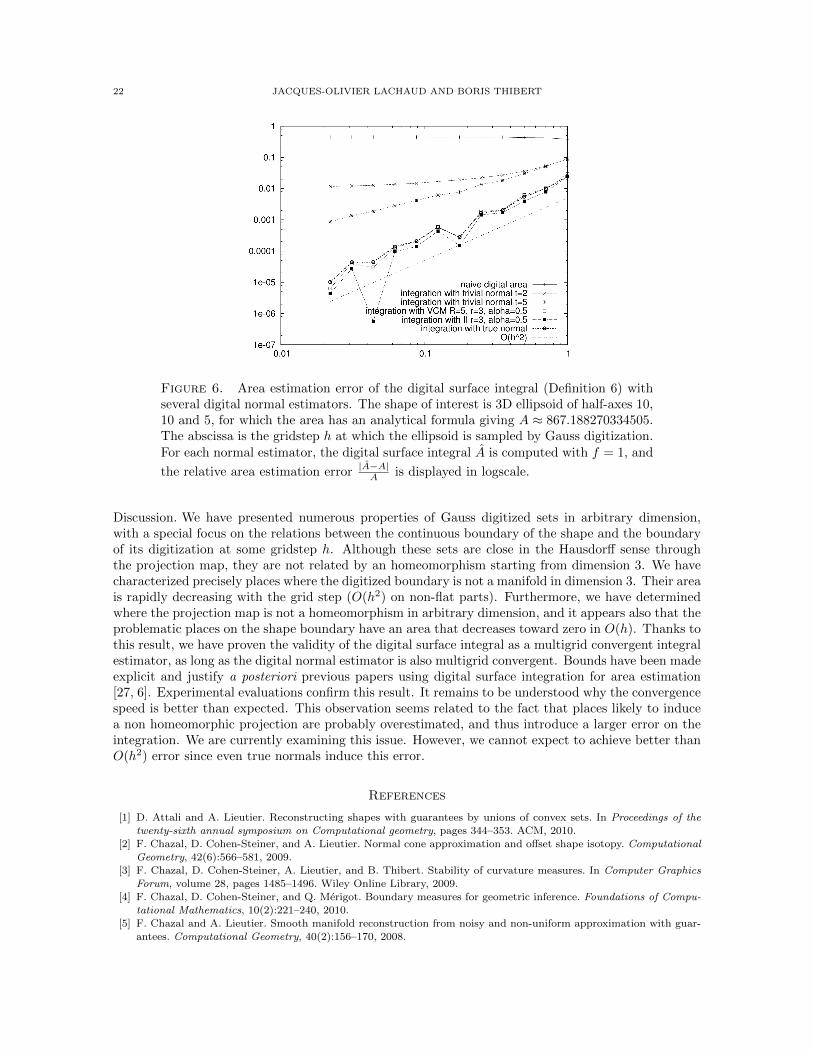
Experimental evaluation. We briefly evaluate numerically the digital surface integral formula for thepurpose of area estimation of a 3D digital shape. Fig. 6 illustrates the area estimation error of digitalsurface integration for several digital normal estimators. Of course, the naive summation of the areasof each 2-cell leads to a non-convergent estimation that overestimates the true area by almost 45%(naive digital area). If the normal is estimated by averaging the trivial cell normals of cells at distanceat most t (called trivial normal of radius t), then better area estimations are obtained (around 1% fort = 2). Still they are not convergent. If we use the exact ellipsoid normals (true normal) or convergentnormal estimators like integral invariants (II, [7, 8]) or Voronoi Covariance Measure (VCM, [10]),then the digital surface integral appears convergent toward the true area. Even better, experimentalconvergence speed looks like O(h2).


Figure 6. Area estimation error of the digital surface integral (Definition 6) withseveral digital normal estimators. The shape of interest is 3D ellipsoid of half-axes 10,10 and 5, for which the area has an analytical formula giving A ≈ 867.188270334505.The abscissa is the gridstep h at which the ellipsoid is sampled by Gauss digitization.For each normal estimator, the digital surface integral A is computed with f = 1, and

the relative area estimation error |A−A|A is displayed in logscale.

Discussion. We have presented numerous properties of Gauss digitized sets in arbitrary dimension,with a special focus on the relations between the continuous boundary of the shape and the boundaryof its digitization at some gridstep h. Although these sets are close in the Hausdorff sense throughthe projection map, they are not related by an homeomorphism starting from dimension 3. We havecharacterized precisely places where the digitized boundary is not a manifold in dimension 3. Their areais rapidly decreasing with the grid step (O(h2) on non-flat parts). Furthermore, we have determinedwhere the projection map is not a homeomorphism in arbitrary dimension, and it appears also that theproblematic places on the shape boundary have an area that decreases toward zero in O(h). Thanks tothis result, we have proven the validity of the digital surface integral as a multigrid convergent integralestimator, as long as the digital normal estimator is also multigrid convergent. Bounds have been madeexplicit and justify a posteriori previous papers using digital surface integration for area estimation[27, 6]. Experimental evaluations confirm this result. It remains to be understood why the convergencespeed is better than expected. This observation seems related to the fact that places likely to inducea non homeomorphic projection are probably overestimated, and thus introduce a larger error on theintegration. We are currently examining this issue. However, we cannot expect to achieve better thanO(h2) error since even true normals induce this error.

References

[1] D. Attali and A. Lieutier. Reconstructing shapes with guarantees by unions of convex sets. In Proceedings of the

twenty-sixth annual symposium on Computational geometry, pages 344–353. ACM, 2010.[2] F. Chazal, D. Cohen-Steiner, and A. Lieutier. Normal cone approximation and offset shape isotopy. Computational

Geometry, 42(6):566–581, 2009.[3] F. Chazal, D. Cohen-Steiner, A. Lieutier, and B. Thibert. Stability of curvature measures. In Computer Graphics

Forum, volume 28, pages 1485–1496. Wiley Online Library, 2009.

[4] F. Chazal, D. Cohen-Steiner, and Q. Merigot. Boundary measures for geometric inference. Foundations of Compu-tational Mathematics, 10(2):221–240, 2010.

[5] F. Chazal and A. Lieutier. Smooth manifold reconstruction from noisy and non-uniform approximation with guar-antees. Computational Geometry, 40(2):156–170, 2008.


[6] D. Coeurjolly, F. Flin, O. Teytaud, and L. Tougne. Multigrid convergence and surface area estimation. In Geometry,

morphology, and computational imaging, pages 101–119. Springer, 2003.[7] D. Coeurjolly, J.-O. Lachaud, and J. Levallois. Integral based curvature estimators in digital geometry. In Discrete

Geometry for Computer Imagery, number 7749 in LNCS, pages 215–227. Springer, 2013.

[8] D. Coeurjolly, J.-O. Lachaud, and J. Levallois. Multigrid convergent principal curvature estimators in digital geom-etry. Computer Vision and Image Understanding, (0):–, 2014. In Press, Corrected Proof, Available online 9 May

2014.

[9] D. Coeurjolly, J.-O. Lachaud, and T. Roussillon. Multigrid convergence of discrete geometric estimators. InValentin E. Brimkov and Reneta P. Barneva, editors, Digital Geometry Algorithms, volume 2 of Lecture Notes

in Computational Vision and Biomechanics, pages 395–424. Springer Netherlands, 2012.[10] L. Cuel, J.-O. Lachaud, and B. Thibert. Voronoi-based geometry estimator for 3d digital surfaces. In Proc. Discrete

Geometry for Computer Imagery (DGCI’2014), Sienna, Italy, Lecture Notes in Computer Science. Springer, 2014.

Accepted. To appear.[11] F. de Vieilleville, J.-O. Lachaud, and F. Feschet. Maximal digital straight segments and convergence of discrete

geometric estimators. Journal of Mathematical Image and Vision, 27(2):471–502, February 2007.

[12] H.-A. Esbelin and R. Malgouyres. Convergence of binomial-based derivative estimation for c2-noisy discretizedcurves. In Proc. 15th DGCI, volume 5810 of LNCS, pages 57–66. 2009.

[13] H.-A. Esbelin, R. Malgouyres, and C. Cartade. Convergence of binomial-based derivative estimation for c2 noisy

discretized curves. Theoretical Computer Science, 412(36):4805–4813, 2011.[14] H. Federer. Curvature measures. Trans. Amer. Math. Soc, 93(3):418–491, 1959.

[15] H. Federer Geometric measure theory. Springer, 1969.

[16] A. Giraldo, A. Gross, and L. J. Latecki. Digitizations preserving shape. Pattern Recognition, 32(3):365–376, 1999.[17] A. Gross and L. Latecki. Digitizations preserving topological and differential geometric properties. Comput. Vis.

Image Underst., 62(3):370–381, 1995.

[18] M. N. Huxley. Exponential sums and lattice points. Proc. London Math. Soc., 60:471–502, 1990.[19] Y. Kenmochi and R. Klette. Surface area estimation for digitized regular solids. In International Symposium on

Optical Science and Technology, pages 100–111. International Society for Optics and Photonics, 2000.[20] R. Klette and A. Rosenfeld. Digital Geometry: Geometric Methods for Digital Picture Analysis. Morgan Kaufmann

Publishers Inc., San Francisco, CA, USA, 2004.

[21] R. Klette and H. J. Sun. Digital planar segment based polyhedrization for surface area estimation. In Visual form2001, pages 356–366. Springer, 2001.

[22] R. Klette and J. Zunic. Multigrid convergence of calculated features in image analysis. Journal of Mathematical

Imaging and Vision, 13(3):173–191, 2000.[23] J.-O. Lachaud. Espaces non-euclidiens et analyse d’image : modeles deformables riemanniens et discrets, topologie

et geometrie discrete. Habilitation a diriger des recherches, Universite Bordeaux 1, Talence, France, 2006.

[24] J.-O. Lachaud, A. Vialard, and F. de Vieilleville. Fast, accurate and convergent tangent estimation on digitalcontours. Image and Vision Computing, 25(10):1572 – 1587, 2007.

[25] L. J. Latecki. 3D well-composed pictures. Graphical Models and Image Processing, 59(3):164–172, May 1997.

[26] L. J. Latecki, C. Conrad, and A. Gross. Preserving topology by a digitization process. Journal of MathematicalImaging and Vision, 8(2):131–159, mar 1998.

[27] A. Lenoir, R. Malgouyres, and M. Revenu. Fast computation of the normal vector field of the surface of a 3-ddiscrete object. In Discrete Geometry for Computer Imagery, pages 101–112. Springer, 1996.

[28] J. Lindblad. Surface area estimation of digitized 3d objects using weighted local configurations. Image and Vision

Computing, 23(2):111–122, 2005.[29] Y.-S. Liu, J. Yi, H. Zhang, G.-Q. Zheng, and J.-C. Paul. Surface area estimation of digitized 3d objects using

quasi-monte carlo methods. Pattern Recognition, 43(11):3900 – 3909, 2010.[30] H. Meine, U. Kothe, and P. Stelldinger. A topological sampling theorem for robust boundary reconstruction and

image segmentation. Discrete Applied Mathematics, 157(3):524–541, 2009.

[31] Q. Merigot, M. Ovsjanikov, and L. Guibas. Voronoi-based curvature and feature estimation from point clouds. IEEE

Transactions on Visualization and Computer Graphics, 17(6):743–756, 2011.[32] J.-M. Morvan. Generalized curvatures, volume 2. Springer, 2008.

[33] P. Niyogi, S. Smale, and S. Weinberger. Finding the homology of submanifolds with high confidence from randomsamples. Discrete & Computational Geometry, 39(1-3):419–441, 2008.

[34] T. Pavlidis. Algorithms for graphics and image processing. Computer science press, 1982.

[35] L. Provot and Y. Gerard. Estimation of the derivatives of a digital function with a convergent bounded error. InDiscrete Geometry for Computer Imagery, pages 284–295. Springer, 2011.

[36] C. Ronse and M. Tajine. Discretization in hausdorff space. Journal of Mathematical Imaging and Vision, 12(3):219–

242, 2000.[37] J. Serra. Image analysis and mathematical morphology. Academic Press, 1982.

[38] M. Siqueira, L. J. Latecki, N. Tustison, J. Gallier, and J. Gee. Topological repairing of 3d digital images. Journal

of Mathematical Imaging and Vision, 30(3):249–274, 2008.


[39] F. Sloboda and J. Stoer. On piecewise linear approximation of planar Jordan curves. J. Comput. Appl. Math.,

55(3):369–383, 1994.[40] P. Stelldinger and U. Kothe. Towards a general sampling theory for shape preservation. Image and Vision Com-

puting, 23(2):237–248, 2005.

[41] P. Stelldinger, L. J. Latecki, and M. Siqueira. Topological equivalence between a 3d object and the reconstructionof its digital image. IEEE Transactions on Pattern Analysis and Machine Intelligence, 29(1):126–140, 2007.

[42] M. Tajine and C. Ronse. Topological properties of hausdorff discretization, and comparison to other discretization

schemes. Theoretical Computer Science, 283(1):243–268, 2002.[43] H. Weyl. On the volume of tubes, American Journal of Mathematics, 61(2):461–472, 1939.

[44] J. Ziegel and M. Kiderlen. Estimation of surface area and surface area measure of three-dimensional sets fromdigitizations. Image and Vision Computing, 28(1):64–77, 2010.

Laboratoire de Mathematiques (LAMA), UMR 5127 CNRS, Universite de Savoie, France

Laboratoire Jean Kuntzmann (LJK), Universite de Grenoble, France

Date post:	10-Nov-2018
Category:	Documents
Upload:	docong
View:	238 times
Download:	0 times

Properties of Gauss digitized sets and digital surface ... · Properties of Gauss digitized sets...

Documents