Emerging market bond spreads: the role of world financial-market conditions and country-specific factors 1 PROSPECTS PAPER A product of the World Bank Development Prospects Group designed to monitor and analyze global economic and financial trends and their implications for developing countries. Emerging market bond spreads: the role of world financial-market conditions and country- specific factors Mike Kennedy and Angel Palerm 1 Introduction and conclusions Emerging market economies have enjoyed increased access to world capital markets over the past few decades, with their borrowing costs in these markets constituting important determinants of their economic development. 2 Since the late 1990’s, these costs (measured as their spreads over US Treasury bonds calculated from JP Morgan’s Emerging Market Bond Index (EMBI + )), while generally trending down, have fluctuated widely (Figure 1). In this paper, for a subset of 18 emerging-market economies, 3 two broad questions will be addressed: To what extent have fluctuations in EMBI + spreads for these economies over the past 8 years been due to the influence of world financial-market conditions compared with home-country developments; and What is the outlook for these EMBI + spreads going forward. 1. The authors’ affiliations are Department of Economics, Queen’s University, Kingston, Ontario and OECD, Paris, respectively. They would like to thank the World Bank for financial support and Andrew Burns, in particular, for first suggesting the topic and for valuable comments as well as Paul Atkinson and Harry Baumann. We would also like to thank Nadia Spivak and Oana Luca of the World Bank for assistance in putting together the database. The OECD also generously provided data on their measure of global risk up to April 2009. The findings, interpretations, and conclusions expressed in this volume do not necessarily reflect the views of the Executive Directors of The World Bank or the governments they represent. The World Bank does not guarantee the accuracy of the data included in this work. Any errors and omissions are attributable to the authors only. 2. See World Bank (2009). 3. The countries to be examined are: Argentina, Brazil, Bulgaria, Chile, China, Colombia, Ecuador, Hungary, Malaysia, Mexico, Panama, Peru, Philippines, Poland, Russia, South Africa, Turkey and Venezuela.
Transcript
Emerging market bond spreads: the role of world financial-market conditions and country-specific factors
1
PROSPECTS PAPER A product of the World Bank Development Prospects Group designed to monitor and analyze global economic and financial trends and their implications for developing countries.
Emerging market bond spreads: the role of world financial-market conditions and country-specific factors
Mike Kennedy and Angel Palerm1
Introduction and conclusions
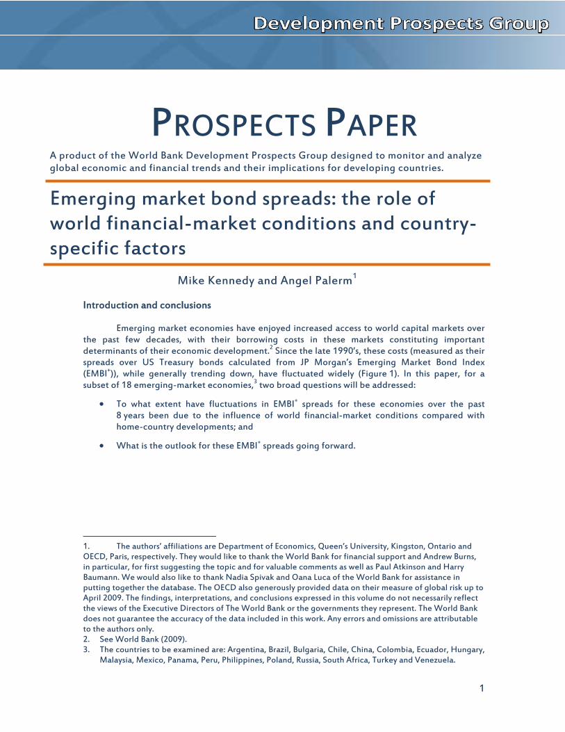
Emerging market economies have enjoyed increased access to world capital markets over the past few decades, with their borrowing costs in these markets constituting important determinants of their economic development.2 Since the late 1990’s, these costs (measured as their spreads over US Treasury bonds calculated from JP Morgan’s Emerging Market Bond Index (EMBI+)), while generally trending down, have fluctuated widely (Figure 1). In this paper, for a subset of 18 emerging-market economies,3 two broad questions will be addressed:
To what extent have fluctuations in EMBI+ spreads for these economies over the past 8 years been due to the influence of world financial-market conditions compared with home-country developments; and
What is the outlook for these EMBI+ spreads going forward.
1. The authors’ affiliations are Department of Economics, Queen’s University, Kingston, Ontario and OECD, Paris, respectively. They would like to thank the World Bank for financial support and Andrew Burns, in particular, for first suggesting the topic and for valuable comments as well as Paul Atkinson and Harry Baumann. We would also like to thank Nadia Spivak and Oana Luca of the World Bank for assistance in putting together the database. The OECD also generously provided data on their measure of global risk up to April 2009. The findings, interpretations, and conclusions expressed in this volume do not necessarily reflect the views of the Executive Directors of The World Bank or the governments they represent. The World Bank does not guarantee the accuracy of the data included in this work. Any errors and omissions are attributable to the authors only. 2. See World Bank (2009). 3. The countries to be examined are: Argentina, Brazil, Bulgaria, Chile, China, Colombia, Ecuador, Hungary,
Malaysia, Mexico, Panama, Peru, Philippines, Poland, Russia, South Africa, Turkey and Venezuela.
Emerging market bond spreads: the role of world financial-market conditions and country-specific factors
2
0
200
400
600
800
1000
1200
1400
1600
1800
Figure 1. Movements in EMBI plus spreads
The approach used here and the main conclusions are:
To address these issues, we follow the literature in assuming that EMBI+ spreads embody the probability of default, which can arise from combinations of market, liquidity and credit risk. In our framework, a single measure of global financial market risk conditions is used to capture both market and liquidity risk faced by emerging markets. Following work at the OECD, global financial market risk conditions are assumed to be captured by the first principal component calculated from a set of yield spreads on assets (bonds and equities) of varying risk in the United States and the euro area, as well as a representative EMBI+ spread.
The resulting variable mirrors quite well what we know about developments in risk conditions (or better still, risk aversion) over the past decade or so in major markets. It, in turn, is well explained by the stance of monetary policy in the United States and the euro area, the outlook for the OECD economy as a whole and a proxy for expected global default rates on corporate bonds. This measure of risk, in turn, was found to be a highly significant determinant of EMBI+ spreads.
To capture credit risk, which reflects an economy’s ability to service its debt, we experimented with a variety of macroeconomic variables for the group of economies under review. Those found to be significant and with the correct sign in an error correction model (estimated using pooled-time series techniques) were a country’s: foreign debt-to-GDP, nominal US dollar GDP growth, CPI inflation and an index of political stability.
Based on simulations using the estimated model for EMBI+ spreads, it is world financial-market risk conditions that play the more important role in accounting for changes in these spreads over the period under study.
While recognising the importance of world risk conditions, the rise in EMBI+ spreads from late 2007 to December 2008 for a majority of the countries studied was actually less than what would have been expected based on past relationships, in many cases significantly so. This could be the result of financial markets giving more weight to domestic developments and/or giving more recognition to the fact that the recent crisis had more to do with developed-country markets. In any event, it can be argued
Emerging market bond spreads: the role of world financial-market conditions and country-specific factors
3
that global financial markets in the most recent episode of deteriorating risk conditions were more discriminating regarding emerging-market economies than in the past, although this does not imply that these economies have de-coupled from global financial markets.
Going forward, the model suggests that EMBI+ spreads for a number of countries could remain low, although they are unlikely to reach past lows seen in January 2007.
The inevitable return of US and euro area policy interest rates towards levels closer to historical averages, as for instance suggested by a Taylor rule, would put upward pressure on these spreads but for a number of emerging market economies, spreads could remain low, especially when compared with recent peaks.
The plan of the rest of the paper is as follows. The next section briefly outlines the basic modelling strategy employed and that section will be followed by a discussion of the proposed measure of world financial-market risk conditions and the factors affecting it. Following that discussion, we present our empirical results on modelling EMBI+ spreads. The subsequent section will use the EMBI+ model to examine what has happened to spreads in these countries over two time periods defined by the decline in world risk conditions starting in late 2002 until mid-2007 and the sharp increase from then to yearend 2008. A final section will use the model to trace developments in EMBI+ spreads over the first half of 2009 for the purposes of providing some estimates of their possible levels going forward. There are as well five appendices (A to E), laying out: the calculation of the global risk measure; a version of the EMBI+ model with country specific coefficients on the risk measure; the short-run constant terms for the model of EMBI+ spreads; how well the model tracks actual spreads; and more details on the simulations discussed in the penultimate section.
The approach to studying EMBI+ spreads
The framework to be used here follows the literature4 and assumes that a particular country’s EMBI+ spread has to be high enough to compensate investors for the probability of default.5 That probability depends on the country’s exposure to market, liquidity and credit risks. Because we are assuming that the economies are small in relation to the world, market risk in our framework is the possibility that the global appetite for risk turns sour, with negative consequences for these economies. Liquidity risk occurs when it becomes difficult to liquidate assets without affecting prices and here again we will assume that this is also related to conditions in global financial markets where emerging-market bonds are traded. Credit risk, on the other hand, is directly related to the ability of a country to service its debts and this is a function of its fundamentals. Putting this together, we assume that investors evaluate the EMBI+ spread for a particular country “i” at time “t” (EMBI+
it) with reference to global financial market risk conditions (to capture the first two types of risk) as well as developments particular to that country (to capture credit risk). Thus:
(1) EMBI+it = f(t, Xij,t),
where t represents global financial-market risk conditions (for simplicity, risk or risk measure hereafter) at time “t”; and Xij,t is a set of “j“ variables for each country “i” also at time “t” that could affect its ability to service its debt.6
4. The seminal work is Edwards (1984). 5. See Cunningham et al. (2001) for a discussion. 6. Another way of thinking about equation (1) is that t represents factors “pushing” funds to emerging
markets while Xij,t captures “pull” effects; see Ferrucci et al. (2004) for a discussion and references to the literature.
Emerging market bond spreads: the role of world financial-market conditions and country-specific factors
4
A feature that differentiates our work from that of others is the definition of t. This variable is meant to represent market and liquidity risks external to emerging market economies. In most work, various separate risk measures are used in regression-analysis, as often as not representing the US markets.7 In contrast, we develop a single risk measure that incorporates these various risks for the US and euro area markets as well as a representative EMBI spread and then we model it. In particular:
(2) t = g(Ykt),
where Ykt represents the various factors that influence global risk conditions.
With this as our framework, the modelling will proceed in two steps, described in the following two sections: in the first, an indicator of t is calculated and then a model of it is estimated; while in the second, the model for EMBI+
it is set out and estimated.
Measuring and modelling global risk
Our first task is to develop a measure of global risk. We start by relying on work done at the OECD where such risk conditions were assumed to be captured by the first principal component computed from a set of spreads on corporate bonds (high grade and high yield) for the United States and the euro area versus their respective government bonds, the implied risk premium on equities for each economy and a representative global EMBI+ spread (shown in Figure 1).8 Using factor analysis to compute a single risk measure has the advantage of measuring the shared movements in these various sub-categories of risky returns and accordingly it captures the broad general directions in world risk conditions.9 While individual movements in various risk subcomponents are missed, their effect has often been hard to identify because of high co-linearity among these asset returns.
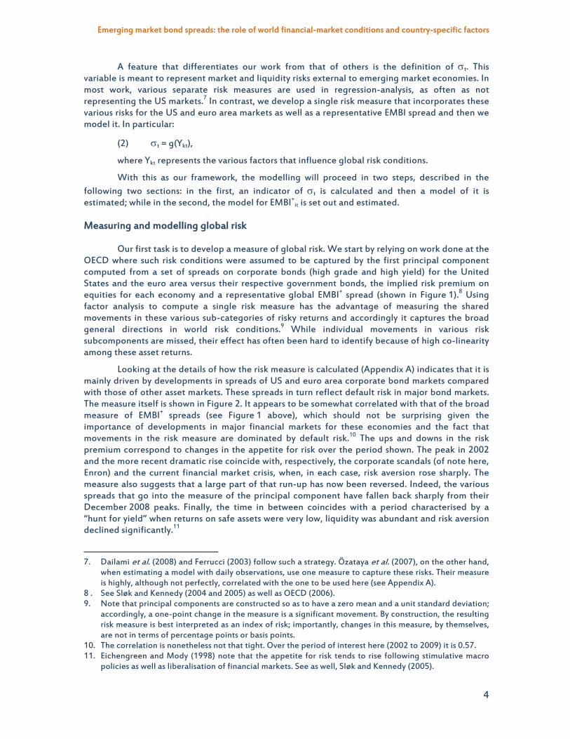
Looking at the details of how the risk measure is calculated (Appendix A) indicates that it is mainly driven by developments in spreads of US and euro area corporate bond markets compared with those of other asset markets. These spreads in turn reflect default risk in major bond markets. The measure itself is shown in Figure 2. It appears to be somewhat correlated with that of the broad measure of EMBI+ spreads (see Figure 1 above), which should not be surprising given the importance of developments in major financial markets for these economies and the fact that movements in the risk measure are dominated by default risk.10 The ups and downs in the risk premium correspond to changes in the appetite for risk over the period shown. The peak in 2002 and the more recent dramatic rise coincide with, respectively, the corporate scandals (of note here, Enron) and the current financial market crisis, when, in each case, risk aversion rose sharply. The measure also suggests that a large part of that run-up has now been reversed. Indeed, the various spreads that go into the measure of the principal component have fallen back sharply from their December 2008 peaks. Finally, the time in between coincides with a period characterised by a “hunt for yield” when returns on safe assets were very low, liquidity was abundant and risk aversion declined significantly.11
7. Dailami et al. (2008) and Ferrucci (2003) follow such a strategy. Özataya et al. (2007), on the other hand,
when estimating a model with daily observations, use one measure to capture these risks. Their measure is highly, although not perfectly, correlated with the one to be used here (see Appendix A).
8 . See Sløk and Kennedy (2004 and 2005) as well as OECD (2006). 9. Note that principal components are constructed so as to have a zero mean and a unit standard deviation;
accordingly, a one-point change in the measure is a significant movement. By construction, the resulting risk measure is best interpreted as an index of risk; importantly, changes in this measure, by themselves, are not in terms of percentage points or basis points.
10. The correlation is nonetheless not that tight. Over the period of interest here (2002 to 2009) it is 0.57. 11. Eichengreen and Mody (1998) note that the appetite for risk tends to rise following stimulative macro
policies as well as liberalisation of financial markets. See as well, Sløk and Kennedy (2005).
Emerging market bond spreads: the role of world financial-market conditions and country-specific factors
5
-2
-1
0
1
2
3
4
5
6
Figure 2. The synthetic measure of the risk premium
To model the risk measure we again follow the OECD, by employing an error correction
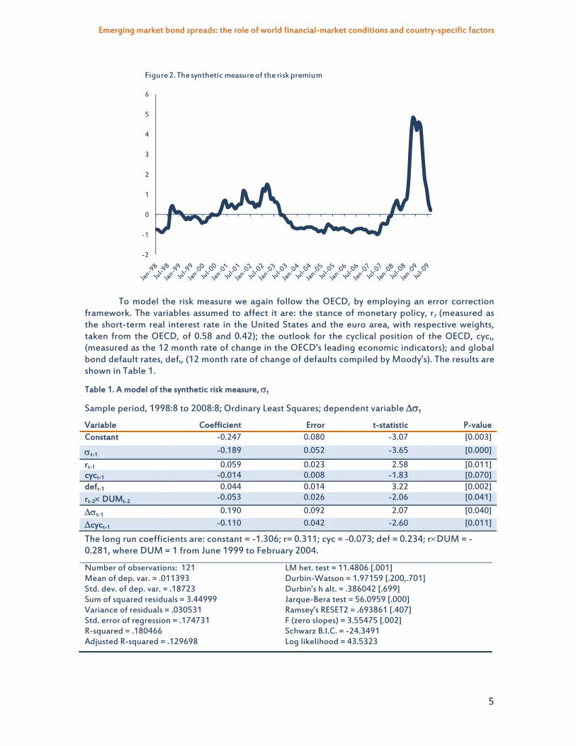
framework. The variables assumed to affect it are: the stance of monetary policy, rt (measured as the short-term real interest rate in the United States and the euro area, with respective weights, taken from the OECD, of 0.58 and 0.42); the outlook for the cyclical position of the OECD, cyct, (measured as the 12 month rate of change in the OECD’s leading economic indicators); and global bond default rates, deft, (12 month rate of change of defaults compiled by Moody’s). The results are shown in Table 1.
Table 1. A model of the synthetic risk measure, t
Sample period, 1998:8 to 2008:8; Ordinary Least Squares; dependent variable t
The long run coefficients are: constant = -1.306; r= 0.311; cyc = -0.073; def = 0.234; rDUM = -0.281, where DUM = 1 from June 1999 to February 2004.
Number of observations: 121 Mean of dep. var. = .011393 Std. dev. of dep. var. = .18723 Sum of squared residuals = 3.44999 Variance of residuals = .030531 Std. error of regression = .174731 R-squared = .180466 Adjusted R-squared = .129698
LM het. test = 11.4806 [.001] Durbin-Watson = 1.97159 [.200,.701] Durbin’s h alt. = .386042 [.699] Jarque-Bera test = 56.0959 [.000] Ramsey’s RESET2 = .693861 [.407] F (zero slopes) = 3.55475 [.002] Schwarz B.I.C. = -24.3491 Log likelihood = 43.5323
Emerging market bond spreads: the role of world financial-market conditions and country-specific factors
6
The short-term real interest rate captures the stance of monetary policy and can be thought of as a proxy for global liquidity risk. The variable cyct, which measures the prospects for the outlook, is included to capture global market risk; any deterioration in the outlook for OECD economies will sour the investment climate. Finally the rate of defaults is a direct measure of what we want and is here used as a proxy for the market’s expectations of default rates; when they rise so does risk aversion and market risk.
A rise in defaults rates, deft, is expected to increase risk while an improvement in the outlook for OECD economies should lower it. The size of the effect of rt proved to be somewhat more difficult to identify statistically. A priori, a tightening of the stance of monetary policy should increase the risk measure; however, over this sample period, there were two periods (around the 2000 recession and more recently) when the relationship between monetary policy and overall risk conditions seemed to break down. Indeed during these periods the correlation between each becomes negative. One possible explanation is that, in an environment of heightened uncertainty, the rapid loosening of monetary policy by the authorities caused financial markets to revise upward sharply their assessment of risk conditions, possibly in recognition that the monetary authorities had better, more timely information. While the inclusion of defaults and the cyclical variable in the equation should in principle go some way to account for such situations, in the work here we found it necessary to include, as a separate variable, the interest rate interacted with a dummy variable to capture such periods.12 Without this variable (which is significant), the coefficient on rt was noticeably smaller and insignificant (although it had the right sign). Note as well that when the two coefficients are taken together, monetary policy appears to be ineffective. This latter variable was not part of the OECD’s work.
In the short-run, changes in the risk measure are also driven by lagged changes in risk as well as lagged changes in the cyclical variable, both of which contribute to the short-run dynamics. We also experimented with different observation periods and found that the relationship was stable up to August 2008. Including the most recent set of observations resulted in a doubling of the SSRs, which is suggestive of a structural break or an end point problem with OLS estimators. In general the fit of the model is good with all variables correctly signed and significant at the 95 per cent level or higher. The exception is the cyclical variable, which is significant at the somewhat lower 93 per cent level. As well the various test statistics suggest no major issues with the equation.
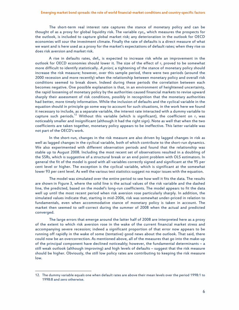
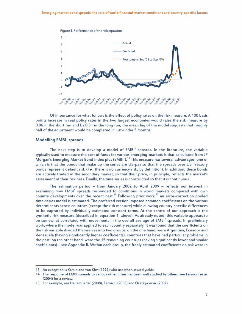
The model was simulated over the entire period to see how well it fits the data. The results are shown in Figure 3, where the solid line is the actual values of the risk variable and the dashed line, the predicted, based on the model’s long-run coefficients. The model appears to fit the data well up until the most recent period when risk aversion rose particularly sharply. In addition, the simulated values indicate that, starting in mid-2006, risk was somewhat under-priced in relation to fundamentals, even when accommodative stance of monetary policy is taken in account. The market then seemed to self-correct during the summer of 2008 when the actual and predicted converged.
The large errors that emerge around the latter half of 2008 are interpreted here as a proxy of the extent to which risk aversion rose in the wake of the current financial market stress and accompanying severe recession; indeed a significant proportion of that error now appears to be running off rapidly in the wake of some (tentative) good news about the outlook. That said, there could now be an overcorrection. As mentioned above, all of the measures that go into the make-up of the principal component have declined noticeably; however, the fundamental determinants – a still weak outlook (although improving) and high levels of defaults – suggest that the risk measure should be higher. Obviously, the still low policy rates are contributing to keeping the risk measure low.
12. The dummy variable equals one when default rates are above their mean levels over the period 1998:1 to
1998:8 and zero otherwise.
Emerging market bond spreads: the role of world financial-market conditions and country-specific factors
7
-2
-1
0
1
2
3
4
5
6
Figure 3. Performance of the risk equation
Actual
Predicted
Post sample (Sep '08 to Sep '09)
Of importance for what follows is the effect of policy rates on the risk measure. A 100 basis points increase in real policy rates in the two largest economies would raise the risk measure by 0.06 in the short run and by 0.31 in the long run; the mean lag of the model suggests that roughly half of the adjustment would be completed in just-under 5 months.
Modelling EMBI+ spreads
The next step is to develop a model of EMBI+ spreads. In the literature, the variable typically used to measure the cost of funds for various emerging-markets is that calculated from JP Morgan’s Emerging Market Bond Index plus (EMBI+).13 This measure has several advantages, one of which is that the bonds that make up the series are US-pay so that the spreads over US Treasury bonds represent default risk (i.e., there is no currency risk, by definition). In addition, these bonds are actively traded in the secondary market, so that their price, in principle, reflects the market’s assessment of their riskiness. Finally, the time series is constructed so that it is continuous.
The estimation period – from January 2002 to April 2009 – reflects our interest in examining how EMBI+ spreads responded to conditions in world markets compared with own country developments over the recent past.14 Following prior work,15 an error-correction pooled time-series model is estimated. The preferred version imposed common coefficients on the various determinants across countries (except the risk measure) while allowing country-specific differences to be captured by individually estimated constant terms. At the centre of our approach is the synthetic risk measure (described in equation 1, above). As already noted, this variable appears to be somewhat correlated with movements in the overall average of EMBI+ spreads. In preliminary work, where the model was applied to each country separately, it was found that the coefficients on the risk variable divided themselves into two groups: on the one hand, were Argentina, Ecuador and Venezuela (having significantly higher coefficients), countries that have had particular problems in the past; on the other hand, were the 15 remaining countries (having significantly lower and similar coefficients) – see Appendix B. Within each group, the freely estimated coefficients on risk were in
13. An exception is Kamin and von Klist (1999) who use when-issued yields. 14. The response of EMBI spreads to various other crises has been well studied by others, see Ferrucci et al.
(2004) for a review. 15. For example, see Dailami et al. (2008), Ferrucci (2003) and Özataya et al. (2007).
Emerging market bond spreads: the role of world financial-market conditions and country-specific factors
8
general not significantly different from each other. Accordingly in what follows, separate coefficients were estimated, one for each group and the data did not reject this restriction.16
To get at credit risk we experimented with a number of domestic country macroeconomic variables, with different lag lengths and in various forms. Country fundamentals tend to move more slowly than the risk measure, especially over the sample period chosen. Here we can profit from pooled estimation methods, which exploit cross-country variation to provide more efficient estimation of coefficients. Then using a general-to-specific approach, in which variables with the lowest levels of significance were eliminated first, the model was whittled down to a set of significant determinants.
Table 2 shows the set of long-run variables found to be significant as well as other variables representing short-run dynamics.17 The long-run coefficients were, in addition to the two risk measures (t-1 and *t-1), a country’s: foreign debt-to-GDP ratio (debt); nominal US dollar growth rate (g); inflation (); and an index of political stability, taken from the International Country Risk Guide database (pol), in which a higher value indicates a more favourable situation.18
In our work, fiscal balances (fis) and import cover (mc) only entered as first differences, implying that they have only a short-run effect.19 It is possible that the long-run effect from fiscal policy is also captured by the debt variable; however, a more likely explanation is that our measure is based on annual data, interpolated to a monthly frequency. A dummy variable to capture the period after Argentina’s default was also included for that country. Perhaps surprisingly, we were unable to find a relationship for the terms of trade. It is possible that its effect is being captured by other variables, like growth and inflation.
16. That a subset of countries have a higher coefficient on the risk variable could reflect non-linearities in
the relationship. Thus, a version of the model was estimated in which the risk measure was interacted with the foreign debt-to-GDP ratio but the coefficients were insignificant. In contrast, Dailami et al. (2008) found a significant relationship when the debt measure was interacted with interest rates.
17. Appendix C contains the values of the short-run coefficients, all of which are significant. 18. On their website, the variable is described as follows: “A means of assessing the political stability of a
country on a comparable basis with other countries by assessing risk points for each of the component factors of government stability, socioeconomic conditions, investment profile, internal conflict, external conflict, corruption, military in politics, religious tensions, law and order, ethnic tensions, democratic accountability, and bureaucracy quality. Risk ratings range from a high of 100 (least risk) to a low of 0 (highest risk), though lowest de facto ratings generally range in the 30s and 40s.”
19. In Ferrucci (2003) the fiscal balance was also found to be insignificant, while Dailami et al. (2008) do not report a fiscal variable.
Emerging market bond spreads: the role of world financial-market conditions and country-specific factors
9
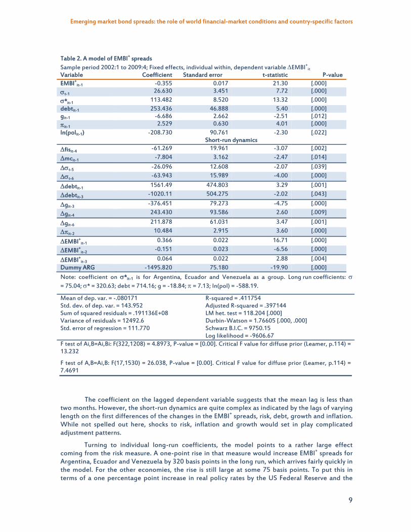
Table 2. A model of EMBI+ spreads Sample period 2002:1 to 2009:4; Fixed effects, individual within, dependent variable EMBI+
it Variable Coefficient Standard error t-statistic P-value EMBI+
Note: coefficient on *it-1 is for Argentina, Ecuador and Venezuela as a group. Long run coefficients: = 75.04; * = 320.63; debt = 714.16; g = -18.84; = 7.13; ln(pol) = -588.19.
Mean of dep. var. = -.080171 Std. dev. of dep. var. = 143.952 Sum of squared residuals = .191136E+08 Variance of residuals = 12492.6 Std. error of regression = 111.770
F test of Ai,B=Ai,Bi: F(322,1208) = 4.8973, P-value = [0.00]. Critical F value for diffuse prior (Leamer, p.114) = 13.232
F test of A,B=Ai,B: F(17,1530) = 26.038, P-value = [0.00]. Critical F value for diffuse prior (Leamer, p.114) = 7.4691
The coefficient on the lagged dependent variable suggests that the mean lag is less than two months. However, the short-run dynamics are quite complex as indicated by the lags of varying length on the first differences of the changes in the EMBI+ spreads, risk, debt, growth and inflation. While not spelled out here, shocks to risk, inflation and growth would set in play complicated adjustment patterns.
Turning to individual long-run coefficients, the model points to a rather large effect coming from the risk measure. A one-point rise in that measure would increase EMBI+ spreads for Argentina, Ecuador and Venezuela by 320 basis points in the long run, which arrives fairly quickly in the model. For the other economies, the rise is still large at some 75 basis points. To put this in terms of a one percentage point increase in real policy rates by the US Federal Reserve and the
Emerging market bond spreads: the role of world financial-market conditions and country-specific factors
10
ECB, based on the risk model (Table 1, above), EMBI+ spreads for the two groups would rise by 100 and 23 basis points respectively. For both groups of countries, this increase is significantly larger than that found by some other authors.20
Foreign indebtedness (debt in Table 2) proved to be very robust to various specifications of the model.21 The higher is a country’s foreign debt level, the more vulnerable it appears to be to a default in the eyes of the market. While a percentage point rise in indebtedness would raise EMBI+ spreads by only 7 basis points (the variable enters as a ratio so that one percentage point is 0.01), the variation in indebtedness has typically been large. The un-weighted average of the 15 countries’ standard deviation of their foreign indebtedness is 0.09, with values ranging from a high of 0.33 for Argentina to a low of 0.007 for China. For the majority of the economies, foreign indebtedness as a ratio of GDP has fallen over the past decade, with most of them having levels of indebtedness in early 2009 at or below their sample means. Exceptions are Hungary and Bulgaria – both have seen increases in their levels of foreign indebtedness to elevated levels.
Growth (g) is an important determinant of EMBI+ spreads, with a higher rate being associated with a better ability to service debt and hence a lower cost of funds. The figures here are interpolated annual US dollar nominal values.22 The actual variable used is a 5-year moving geometric average of annual growth rates so as to capture the underlying performance of the economy. US dollar values are a good measure of a country’s ability to service its obligations. A number of these economies have witnessed significant improvements in growth rates so measured over the past decade or so, notably Argentina, Panama and Peru. Of the group, China has had the best performance while activity in Venezuela has virtually stalled and that of Ecuador has slowed significantly. The remaining countries in the sample have recorded improvements at the end of the sample period, compared with their means over this period.
Inflation is often interpreted as a proxy for macroeconomic policy management as well as an indicator of balance of payment risk. The declines in inflation registered by a large number of emerging market economies has been one the success stories for this group of economies and this has improved their access to international debt markets over the past two decades. Over the sample period, inflation has stayed close to its mean level for most of these economies with notable improvements seen by Argentina and Turkey. On the other hand, Venezuela and Russia have more recently experienced important increases in inflation rates.
The political variable captures such aspects as good governance and corruption or the lack thereof (see footnote 18). It is helpful in determining cross-country differences in risk perception on the part of investors. Particular high scores are recorded for Chile, Hungary and Poland while Venezuela, followed by Ecuador and Colombia have relatively low scores on this measure. Indeed, using Chile and Venezuela as examples, in April 2009, differences in their political scores meant that Chile’s EMBI+ spreads were 290 basis points lower than Venezuela’s.
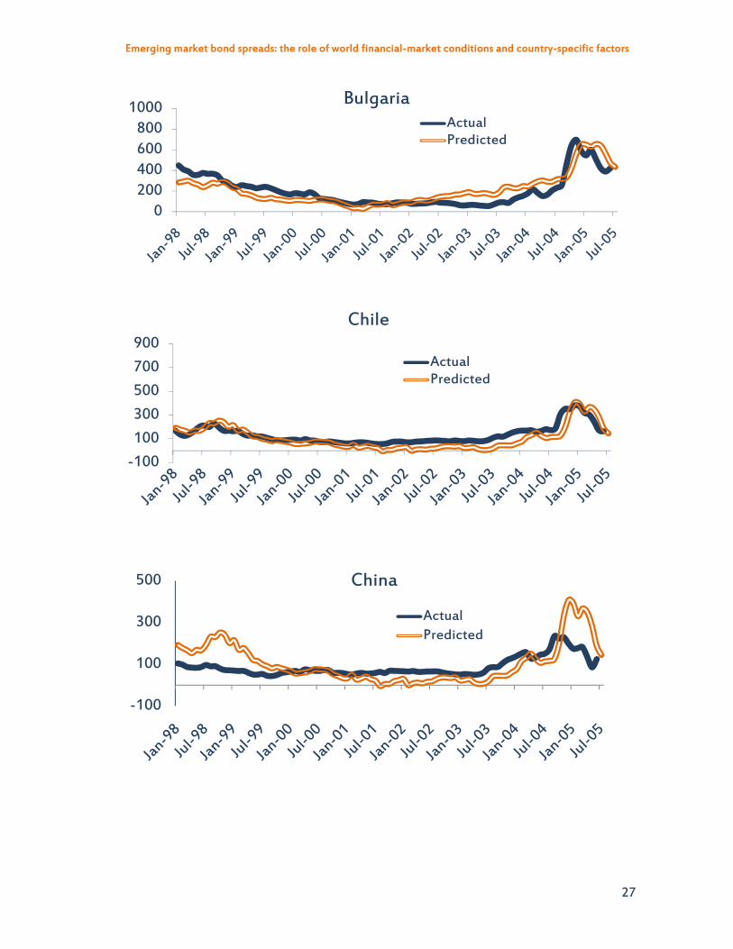
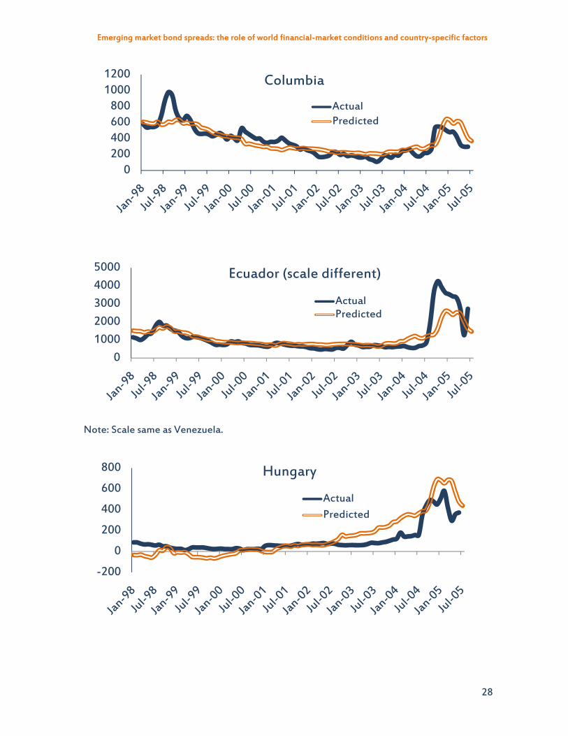
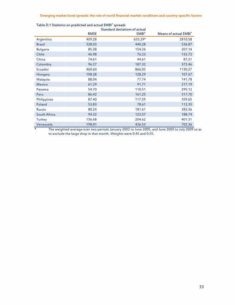
How well the model tracks actual spreads is shown graphically for each country in Appendix D. Table D.1 in that Appendix shows the root mean squared errors (RMSE) of the model’s predictions along with the individual standard deviations and means of the EMBI+ spreads. With the exception of China and Malaysia, the RMSE is less than the standard deviation. In general the overall performance is quite good. For most countries the model follows actual movements fairly closely. Exceptions are Brazil, Hungary and to lesser extents, Bulgaria and Malaysia. There is as well a tendency to over-predict the recent run up in spreads in several cases. Exceptions are Ecuador,
20. For instance, Dailami et al. (2008), estimated increases of 32 basis points for highly indebted economies
following a 100 basis point increase in US policy rates. Ferrucci (2003) estimates a somewhat larger effect while Kamin and von Klist (1999), using a different data set find very little effect coming from major country policy rates.
21. Data are from the World Bank except for Hungary, which are cumulated current account balances. 22. Using interpolated data does impose some linearity on the model.
Emerging market bond spreads: the role of world financial-market conditions and country-specific factors
11
Russia and South Africa where spreads where higher than what would have been suggested by the model.
Explaining movements in EMBI+ spreads over the recent past
A recurring theme in the literature is the extent to which EMBI+ spreads are sensitive to movements in financial conditions in major markets compared with fundamentals.23 The past 8 years, during which the risk measure has seen large changes, provides a good test as these largely originated in major countries. After reaching a near-term peak in late 2002, in the wake of the corporate scandals that seemed to affect a large number of risky asset classes, the risk measure declined sharply up until mid-2007. A year or so after that, as the recession took hold and the financial crisis deepened, it backed up very sharply as a general climate of heightened risk aversion became more and more pervasive. In the following subsections we use the model to calculate how much of the movements in the risk measure and other factors affected EMBI+ spreads during these two periods.
Factors driving the declines: October 2002 to July 2007
Figure 4 provides an overview of what happened to EMBI+ spreads over the period from October 2002, when many of them had hit peaks, to their trough in mid 2007. Argentina, followed by Brazil, Ecuador and Colombia, witnessed the largest drops in spreads, while Hungary and China, whose EMBI+ spread were very low in late 2002, saw the smallest declines. Several of these countries witnessed drops of between 500 and 1000 basis points.
Note: data is in terms of basis points.
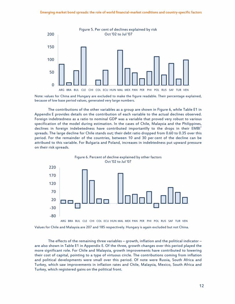
Figure 5 presents the percentage amount of the actual decline explained by movements in the risk measure alone. To make the Figure readable, it was necessary to exclude China and Hungary; the model suggests a decline of 180 basis points for China and Hungary compared with actual drop of 38 basis points for China and a tiny increase of 6 basis point for Hungary, which results in a huge percentage explained. Turning to the other countries, in the case of Argentina, a large part of the decline is attributable to the dummy variable (see Table 2) which captures their improved access to financial markets following their default in 2002. Here it is implicitly assumed that this is a reduction in their riskiness. For eleven of the remaining countries, 50 per cent or more of the decline can be accounted for by changes in the risk measure and for a few countries – Poland, South Africa and Venezuela – most of the declines. The declines in spreads are over-explained, for Chile and Malaysia by a margin of 51 and 38 per cent, respectively.
23 . See Calvo (2005) for a review as well as a discussion of a number of policy issues.
0
2000
4000
6000
8000
ARG BRA BUL CLE CHI COL ECU HUN MAL MEX PAN PER PHI POL RUS SAF TUR VEN
Figure 4. Actual declines in EMBI spreads Oct '02 to Jul '07 (absolute values)
Emerging market bond spreads: the role of world financial-market conditions and country-specific factors
12
Note: values for China and Hungary are excluded to make the figure readable. Their percentage explained, because of low base period values, generated very large numbers.
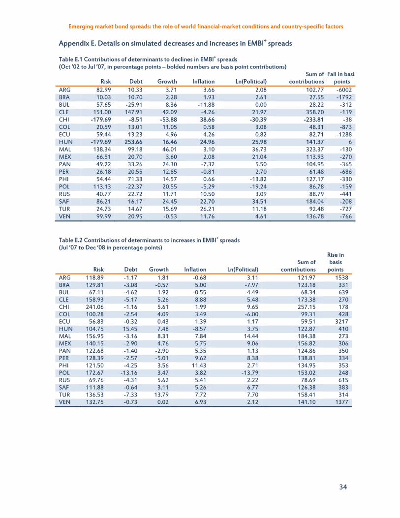
The contributions of the other variables as a group are shown in Figure 6, while Table E1 in Appendix E provides details on the contribution of each variable to the actual declines observed. Foreign indebtedness as a ratio to nominal GDP was a variable that proved very robust to various specification of the model during estimation. In the cases of Chile, Malaysia and the Philippines, declines in foreign indebetedness have contributed importantlly to the drops in their EMBI+
spreads. The large decline for Chile stands out; their debt ratio dropped from 0.60 to 0.35 over this period. For the remainder of the countries, between 10 and 30 per cent of the decline can be attribued to this variable. For Bulgaria and Poland, increases in indebtedness put upward pressure on their risk spreads.
Values for Chile and Malaysia are 207 and 185 respectively. Hungary is again excluded but not China.
The effects of the remaining three variables – growth, inflation and the political indicator – are also shown in Table E1 in Appendix E. Of the three, growth changes over this period played the more significant role. For Chile and Malaysia, growth improvements have contributed to lowering their cost of capital, pointing to a type of virtuous circle. The contributions coming from inflation and political developments were small over this period. Of note were Russia, South Africa and Turkey, which saw improvements in inflation rates and Chile, Malaysia, Mexico, South Africa and Turkey, which registered gains on the political front.
0
50
100
150
200
ARG BRA BUL CLE CHI COL ECU HUN MAL MEX PAN PER PHI POL RUS SAF TUR VEN
Figure 5. Per cent of declines explained by riskOct '02 to Jul '07
-80
-30
20
70
120
170
220
ARG BRA BUL CLE CHI COL ECU HUN MAL MEX PAN PER PHI POL RUS SAF TUR VEN
Figure 6. Percent of decline explained by other factors Oct '02 to Jul '07
Emerging market bond spreads: the role of world financial-market conditions and country-specific factors
13
One key message to take away from the above is the important role that risk and, to a certain extent, foreign indebtedness play in determining EMBI+ spreads. In the majority of cases these two variables, which are obviously related, play the dominant role in explaining movements in EMBI+ spreads over this period, with South Africa and Turkey being exceptions. The other message is that in several cases the model over-explains the declines in spreads; that is, based on the handful of determinants used here, spreads should have fallen by more. This is true for Chile, Malaysia, the Philippines, South Africa and Venezuela. One explanation is that the financial markets are using additional information to that included here in evaluating spreads.24 The other explanation is that emerging markets were not being given enough credit for fundamental developments.
Factors behind the increases: July 2007 to December 2008
From mid- to late 2007, the financial-market risk measure started to adjust upward from its very low levels but from late 2008 the rise accelerated sharply as the financial crisis deepened, finally peaking in December of that year. EMBI+ spreads were not spared and some countries (Argentina, Ecuador and Venezuela) saw particularly sharp increases (Figure 7). This subsection will mirror the preceding, using the model’s parameters to account for the changes over this period.
Note: data is in terms of basis points.
As above, we start by calculating the effect that changes in the risk measure had on various
EMBI+ spreads. The results are shown in Figure 8. Even more than in the previous case, changes in the risk measure play the dominant role, in several countries explaining all or even more than all of the change. Even in the case of Ecuador and Russia, the measure accounts for more than 50 per cent of the run-up in spreads. Of interest here is that the model suggests, based on past relationship, that changes in global risk conditions should have increased EMBI+ spreads by much more in the majority of countries studied here (Argentina, Brazil, Chile, China, Malaysia, Mexico, Panama, Peru, the Philipinnes, Poland and Venezuela).
24. For a similar argument see Ferrucci (2003).
0
500
1000
1500
2000
2500
3000
3500
ARG BRA BUL CLE CHI COL ECU HUNMAL MEX PAN PER PHI POL RUS SAF TUR VEN
Figure 7. Actual increases in EMBI spreads Jul '07 to Dec '08(absolute values)
Emerging market bond spreads: the role of world financial-market conditions and country-specific factors
14
Note: Values for China and Poland are 241 and 173 respectively.
The effects of all the other determinants (excluding risk) of EMBI+ spreads are shown as a group in Figure 9. The next important determinant is foreign debt and here, while improvements in debt positions helped to soften the blow coming from deteriorating financial market conditions, the effect was marginal, on the order of 5 basis points or less (Table E2, Appendix E). Poland’s improved debt position helped to restrain increases in its spreads by 13 basis points. Hungary on the other hand saw a deterioration in its debt position, which pushed up yields by some 15 basis points. Part of the reason for the small effect is that the debt-to-GDP measure is a more slow-moving variable and the period under consideration is short.
Comparing Figures 8 and 9, the role of risk is again dominant, explaining (sometimes over-
explaining) changes in the spreads. This should not be too surprising given that the time period, at 18 months, is short and the risk measure moved the most. Nevertheless, combined with the results obtained when looking at declines, it does point to the key role that the risk measure pays.25
25. This result is consistent with those of others, with the exception of Kamin and von Klist (1999) and has
been labelled at the “globalisation hazard” by Calvo (2002).
0
50
100
150
200
250
ARG BRA BUL CLE CHI COL ECU HUN MAL MEX PAN PER PHI POL RUS SAF TUR VEN
Figure 8. Per cent of increase explained by risk Jul '07 to Dec '08
-30
-20
-10
0
10
20
30
ARG BRA BUL CLE CHI COL ECU HUN MAL MEX PAN PER PHI POL RUS SAF TUR VEN
Figure 9. Percent of increase explained by other factors Jul '07 to Dec '08
Emerging market bond spreads: the role of world financial-market conditions and country-specific factors
15
Another conclusion from this exercise is that the overall increases in EMBI+ spreads for a majority of these countries were less than what would have occurred based on past relations with the global risk measure. In this regard, many emerging market avoided some part of the worst of the run-up in risk aversion that occurred in developed countries (comparing Figures 1 and 2, the run-up in the risk meaure is much sharper than that of total EMBI+ spreads). A possible conclusion is that, as in the case of the declines, financial markets may have been using more information than contained in the model to assess spreads. This could include the fact that the recent crisis was for the most part due to developments particular to developed market economies. In general, credit risk proxies in emerging markets performed well in the circumstances, and markets may have placed more weight on them than suggested by past relationships. What is interesting is that this seems to represent a break with the past when emerging markets typcially developed pneumonia when the major economies caught a cold. This is not meant to imply that these markets have de-coupled from developments in major financial markets. In fact, quite the opposite is case given the importance of the risk measure as an explanitory variable, which is largely driven by developments in major financial markets.
The role of risk and its implications going forward
In this section, we wish to shed some light on the question of where various countries’ EMBI+ spreads are going. To establish points of departure we will use the model to trace developments in the level of EMBI+ spreads for December 2008, the point when the global risk measure reached a peak (as did several EMBI+ spreads); April 2009, the last point for which we have a complete set for the various determinants; and July 2009, where we have information only on spreads and the risk measure. The purpose is to develop an idea as to where actual spreads are in relation to fundamentals and what level they might converge to going forward. While we will not be describing the role of each determinant, it is changes in risk that account for most of the movements in EMBI+ spreads seen over this period and movements in it are likely to be the most important factor going forward in the short term.
Developments in EMBI+ from December 2008 to July 2009
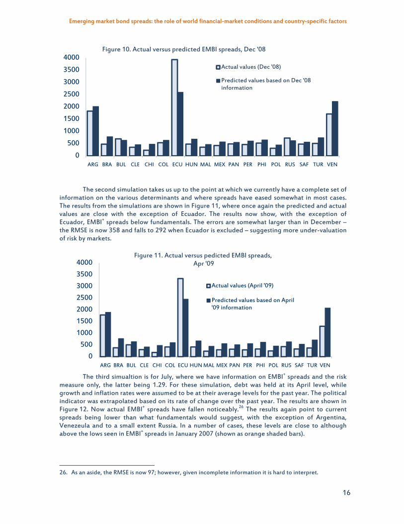
The results of using the model to estimate the December levels for the various countries compared with their actual values are shown in Figure 10. The model performs reasonably well for all countries, considering that a rather rich set of dynamics is excluded. The exception is Ecuador, which registers a very large error. The overall RMSE, calculated across countries at this point in time, is 370, but it falls to 194 when Ecuador is excluded from the sample. For comparison the SER is 111.8. In most cases, the model over-predicts actual levels, which, taken at face value, suggests that markets under-priced risk at that point, a fact that is consistent with what we found in the previous section. The results suggest that markets are pricing in a substantial amount of extra risk in the case of Ecuador and a small amount in the cases of Bulgaria and Russia.
Emerging market bond spreads: the role of world financial-market conditions and country-specific factors
16
The second simulation takes us up to the point at which we currently have a complete set of information on the various determinants and where spreads have eased somewhat in most cases. The results from the simulations are shown in Figure 11, where once again the predicted and actual values are close with the exception of Ecuador. The results now show, with the exception of Ecuador, EMBI+ spreads below fundamentals. The errors are somewhat larger than in December – the RMSE is now 358 and falls to 292 when Ecuador is excluded – suggesting more under-valuation of risk by markets.
The third simualtion is for July, where we have information on EMBI+ spreads and the risk
measure only, the latter being 1.29. For these simulation, debt was held at its April level, while growth and inflation rates were assumed to be at their average levels for the past year. The political indicator was extrapolated based on its rate of change over the past year. The results are shown in Figure 12. Now actual EMBI+ spreads have fallen noticeably.26 The results again point to current spreads being lower than what fundamentals would suggest, with the exception of Argentina, Venezeula and to a small extent Russia. In a number of cases, these levels are close to although above the lows seen in EMBI+ spreads in January 2007 (shown as orange shaded bars).
26. As an aside, the RMSE is now 97; however, given incomplete information it is hard to interpret.
0
500
1000
1500
2000
2500
3000
3500
4000
ARG BRA BUL CLE CHI COL ECU HUN MAL MEX PAN PER PHI POL RUS SAF TUR VEN
Figure 10. Actual versus predicted EMBI spreads, Dec '08
Actual values (Dec '08)
Predicted values based on Dec '08 information
0
500
1000
1500
2000
2500
3000
3500
4000
ARG BRA BUL CLE CHI COL ECU HUN MAL MEX PAN PER PHI POL RUS SAF TUR VEN
Figure 11. Actual versus pedicted EMBI spreads,Apr '09
Actual values (April '09)
Predicted values based on April '09 information
Emerging market bond spreads: the role of world financial-market conditions and country-specific factors
17
Developments in EMBI+ spreads over the near term
As a final exercise, we will concentrate on the values to which EMBI+ spreads may converge over the near term based on where the risk premium may settle and close by speculating on the levels to which the 18 countries’ interest rates may end up. According to the risk model in Table 1, its long-run value would depend upon the equilibrium values of policy rates, the OECD’s cyclical position and default rates. The easiest way forward is to assume that these variables revert back to their mean levels from January 1998 to August 2008. Excluded here are the most recent observations, which are assumed to be outliers. These values are: for the 12-month rate of change of the OECD’s leading economic indicators, 1.7; and for defaults, 4.4. For policy rates, the average was taken from 1997 to mid 2001, yielding a rate of 2.9, which seems more in line with what a Taylor rule might predict. This yielded an equilibrium value for the risk measure of 0.488, which lies between it’s September estimated level of 0.216 and the July level of 1.29. In this simulation we assume the same values for the other determinants as shown in Figures 12 above. Reference points are again the July levels (shown as light blue bars) and the lows EMBI+ spreads reached in January 2007 (shown as orange bars) while the scale remains the same as in the previous two figures.
The results are shown in Figure 13. For all countries, the model suggests that spreads would stay above their previous lows seen in late 2007 (in the cases of Argentina, Ecuador and Venezuela, substantially above those lows, reflecting their sensitivity to the global risk measure) and for the most part remain close to their July levels. For Argentina and Venezuela, spreads could ease from recent levels.
0
1000
2000
3000
4000
ARG BRA BUL CLE CHI COL ECU HUN MAL MEX PAN PER PHI POL RUS SAF TUR VEN
Figure 12. Actual versus predicted EMBI spreads, Jul '09
Actual values (Jul '09)
Predicted values based on Jul '09 information
EMBI lows Jan '07
0
1000
2000
3000
4000
ARG BRA BUL CLE CHI COL ECU HUNMAL MEX PAN PER PHI POL RUS SAF TUR VEN
Figure 13. EMBI spreads when risk moves back to its equilibrium level
EMBI recent Jul '09Predicted based on Jul '09 information and risk spread of 0.488EMBI lows Jan '07
Emerging market bond spreads: the role of world financial-market conditions and country-specific factors
18
All of these countries are at risk of a backup in risk conditions. Indeed, the actual (September) level of the risk measure is significantly lower than estimated by the risk equation suggesting that it may have overshot its near-term value. As already discussed, a one-point rise in this measure would have the largest effect on Argentina, Ecuador and Venezuela (320 basis points). The other countries would see a rise of 75 basis points and, in general, they could weather such an increase.
There are three identified factors that could cause the risk premium to backup, including, a rise in policy rates, a deterioration in the outlook and an increase in default rates. With the major economies now showing signs of exiting from the current recession, the monetary authorities will have to begin the process of withdrawing the large amount of stimulus that was put in place to combat the recession. Provided that process proceeds smoothly, risk conditions should continue to improve. However, if there was a need to tighten the stance of monetary policy sharply, risk conditions would as well rise sharply, possibly overshooting fundamentals with consequences for EMBI+ spreads, particularly for the three countries already noted. Any deterioration in the outlook or a rise in defaults would affect all spreads.
The question as to the level of interest rates these countries may converge depends ultimately on the equilibrium level of US 10 year Treasury rates, on which EMBI+ spreads are based. In Figure 14, two levels are shown. In the first, we have applied the spreads shown in Figure 13 to the current (October) level of US 10-year Treasuries of 3½ per cent. The results are shown as the solid bars.
Such levels are of course unrealistic as they assume that US long rates stay at current levels. They are shown simply to provide a benchmark. The second calculation assumes a US long-term interest rate of 5.2%, based on a potential growth rate of 2½ per cent, an inflation rate of 2 per cent and a yield curve premium of 0.7 per cent. These levels are shown as the clear bars in Figure 14. The differences between each is a rough and ready measure of the amount by which long-term borrowing costs could rise in each country (170 basis points, by construction) and the levels to which they would converge, assuming no change in the various fundamentals underlying the spreads calculated in Figure 13, above. In a number of cases – Argentina, Brazil, Ecuador and Venezuela – borrowing rates could be close to or exceed 10 per cent.
0
5
10
15
20
ARG BRA BUL CLE CHI COL ECU HUN MAL MEX PAN PER PHI POL RUS SAF TUR VEN
Figure 14. Levels of emerging market bond interest rates under two assumptions
US 10 year rate = 3.5% US 10 year rate = 5.2%
Emerging market bond spreads: the role of world financial-market conditions and country-specific factors
19
References: Calvo, G (2002), “Globalization hazard and delayed reform in emerging markets”, Economica 2(2).
Calvo, G (2005), “Crisis in emerging market economies: A global perspective”, NBER Working Paper no. 11305.
Cunningham, A, L Dixon and S Hayes (2001), “Analysing yield spreads on emerging market sovereign bonds”, Bank of England Financial Stability Review.
Dailami, M, P R Masson and J J Padou (2008), “Global monetary conditions versus country-specific factors in the determination of emerging market debt spreads”, Journal of International Money and Finance, Vol 20(1).
Edwards, S (1984), “LDC foreign borrowing and default risk: An empirical investigation, 1976-80”, American Economic Review Vol 74, no 4.
Eichengreen, B and A Mody (1998), “ What explains changing spreads on EM debt: Fundamentals or market sentiment?” NBER Working Paper, no. 6408.
Ferrucci, G, V Herzberg, F Soussa and A Taylor (2004), “Understanding capital flows to emerging market economies”, Bank of England Financial Stability Review.
Ferrucci, G (2003), “Empirical determinants of emerging market economies’ bond spreads”, Bank of England Working Paper, no. 205.
Kamin, S and K von Klist (1999), “The evolution and determinants of emerging market credit spreads in the 1990s”, BIS Working Papers, no. 68.
OECD (2006), “The OECD’s indicator of risk premiums”, Appendix I.2, OECD Economic Outlook No. 80, December 2006.
Özataya, F, E Özmenb and G Şahinbeyoğluc (2007), “Emerging market sovereign spreads, global financial conditions and US macroeconomic news”, ERC Working Papers in Economics, Economic Research Center, Middle East Technical University, Ankara, Turkey.
Sløk, T and M Kennedy (2004), “Factors driving risk premia”, OECD Economics Department Working Papers, no. 385.
Sløk, T and M Kennedy (2005), “Explaining risk premia on bonds and equities”, OECD Economic Studies, no. 40.
World Bank (2009), “Longer-term implications of the financial crisis for growth in developing countries “, Chapter 2, Global Economic Prospects.
Emerging market bond spreads: the role of world financial-market conditions and country-specific factors
20
Appendix A: Calculating and updating the OECD’s risk measure
The method
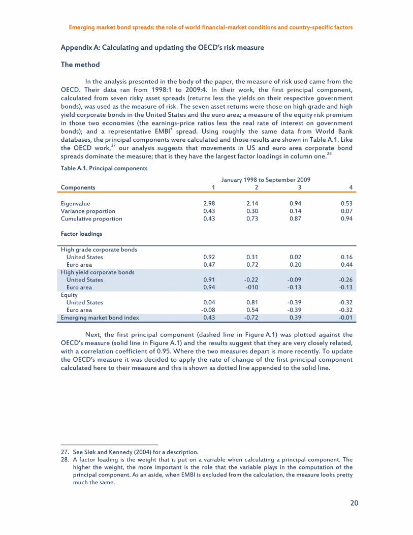
In the analysis presented in the body of the paper, the measure of risk used came from the OECD. Their data ran from 1998:1 to 2009:4. In their work, the first principal component, calculated from seven risky asset spreads (returns less the yields on their respective government bonds), was used as the measure of risk. The seven asset returns were those on high grade and high yield corporate bonds in the United States and the euro area; a measure of the equity risk premium in those two economies (the earnings-price ratios less the real rate of interest on government bonds); and a representative EMBI+ spread. Using roughly the same data from World Bank databases, the principal components were calculated and those results are shown in Table A.1. Like the OECD work,27 our analysis suggests that movements in US and euro area corporate bond spreads dominate the measure; that is they have the largest factor loadings in column one.28
Table A.1. Principal components
January 1998 to September 2009 Components 1 2 3 4 Eigenvalue 2.98 2.14 0.94 0.53 Variance proportion 0.43 0.30 0.14 0.07 Cumulative proportion
0.43 0.73 0.87 0.94
Factor loadings
High grade corporate bonds United States 0.92 0.31 0.02 0.16 Euro area 0.47 0.72 0.20 0.44 High yield corporate bonds United States 0.91 -0.22 -0.09 -0.26 Euro area 0.94 -010 -0.13 -0.13 Equity United States 0.04 0.81 -0.39 -0.32 Euro area -0.08 0.54 -0.39 -0.32 Emerging market bond index 0.43 -0.72 0.39 -0.01
Next, the first principal component (dashed line in Figure A.1) was plotted against the OECD’s measure (solid line in Figure A.1) and the results suggest that they are very closely related, with a correlation coefficient of 0.95. Where the two measures depart is more recently. To update the OECD’s measure it was decided to apply the rate of change of the first principal component calculated here to their measure and this is shown as dotted line appended to the solid line.
27. See Sløk and Kennedy (2004) for a description. 28. A factor loading is the weight that is put on a variable when calculating a principal component. The
higher the weight, the more important is the role that the variable plays in the computation of the principal component. As an aside, when EMBI is excluded from the calculation, the measure looks pretty much the same.
Emerging market bond spreads: the role of world financial-market conditions and country-specific factors
21
Some authors have proposed other measures of global risk, one of which is the use of the Chicago Board of Trade’s index of implied volatilities taken from options on the S&P index (VIX).29 Figure A.2 shows that measure with the one used here. As can been seen, the risk measure developed here has a lot of the same information as the VIX (the correlation coefficient is .74 over the period) but in addition it does incorporate more information that is directly related to bond spreads, which are more closely related to EMBI+ spreads.
29. In a regression using daily data, Özataya, et al. (2006) employ the VIX as a measure of global financial
market conditions and found it to be a significant determinant of EMBI+ spreads.
-2
-1
0
1
2
3
4
5
6 Figure A.1 Updating the risk measure
OECD series
Estimated with 7 risk measures
Updated series
-2
-1
0
1
2
3
4
5
6
0
10
20
30
40
50
60
70Figure A.2 The risk measure versus implied volatility
Implied volaility index (left scale)
Risk measure
Emerging market bond spreads: the role of world financial-market conditions and country-specific factors
22
Appendix B. The model with country specific coefficients on the risk measure
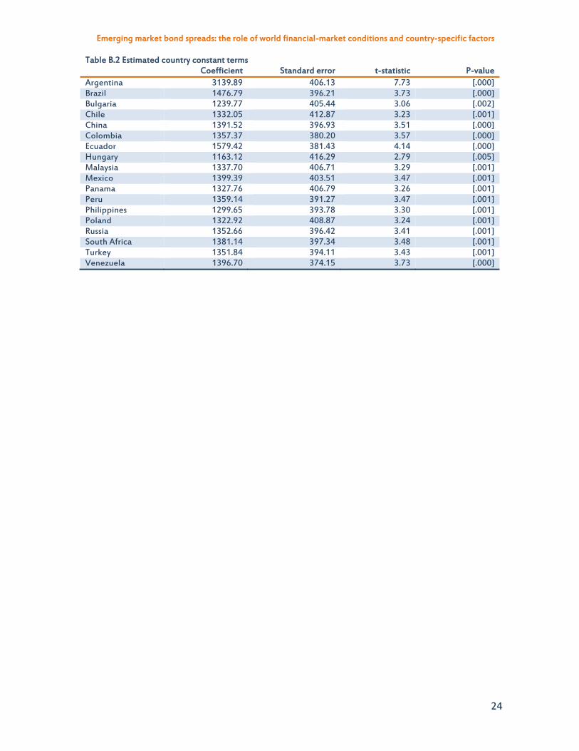
In this Appendix we show the model in Table 2 of the main text except that now we allow for country-specific coefficients on the risk measure (Table B.1). For completeness, Table B.2 contains the individual constant terms for each country.
Looking at the results in Table B.1, it can be seen that the coefficients on the risk measure divide themselves into two groups consisting of, on the one hand, Argentina, Ecuador and Venezuela with significantly higher coefficients and, on the other hand, the remaining 15 countries, with lower coefficients that are not significantly different from each other. These are presented in Figure B.1 below. Looking at the high risk coefficients, a case can be made for treating Ecuador separate from Argentina and Venezuela, although interesting the data seems to have accepted the constaint imposed in the Table 2 version.
Of interest is that fact the F-test does not reject the constraint imposed by having common coefficients on all variables other than the risk measure. That said, in this version of the model, the coefficients on growth and the fiscal variable are now insignificant, although they retain the correct signs. As for foreign debt, inflation and the political risk variable, they are not only significant but have magnitudes similar to those shown in Table 2. This suggests that the version presented here is a viable alternative to the one shown in Table 2.
0
50
100
150
200
250
05
101520253035404550
BRA BUL CLE CHI COL HUN MAL MEX PAN PER PHI POL RUS SAF TUR Risk ARG ECU VEN Risk high
High risk coefficientsRisk coefficients
Figure B.1. Freely estimated (light blue bars) versus constrained risk (dark blue bars) coefficients
Emerging market bond spreads: the role of world financial-market conditions and country-specific factors
23
Table B.1 A model of EMBI+ spreads with country specific risk coefficients Sample period 2002:1 to 2009:4; Fixed effects, individual within, dependent variable EMBI+
it Variable Coefficient Standard error t-statistic p-value EMBI+
it-1 -0.408 0.017 -23.70 [.000] it-1 ARG 113.892 11.854 9.61 [.000] BRA 42.030 9.525 4.41 [.000] BUL 37.824 9.552 3.96 [.000] CLE 19.196 9.619 2.00 [.046] CHI 22.682 9.500 2.39 [.017] COL 32.890 9.486 3.47 [.001] ECU 230.117 13.345 17.24 [.000] HUN 32.328 9.438 3.42 [.001] MAL 25.816 9.535 2.71 [.007] MEX 25.301 9.410 2.69 [.007] PAN 29.524 9.689 3.05 [.002] PER 28.467 9.438 3.02 [.003] PHI 24.071 9.473 2.54 [.011] POL 31.819 9.563 3.33 [.001] RUS 39.160 9.701 4.04 [.000] SAF 22.252 9.542 2.33 [.020] TUR 18.648 10.184 1.83 [.067] VEN 102.283 12.276 8.33 [.000] debtit-1 312.380 47.174 6.62 [.000] git-1 -2.847 2.683 -1.06 [.289] it-1 2.798 0.627 4.46 [.000] ln(polit-1) -322.690 93.989 -3.43 [.001] Short-run dynamics
fisit-4 -25.396 20.671 -1.23 [.219]
mcit-1 -6.901 3.096 -2.23 [.026]
t-5 -30.538 12.316 -2.48 [.013]
t-6 -71.100 15.614 -4.55 [.000]
debtit-1 1305.670 464.920 2.81 [.005]
debtit-3 -581.985 500.053 -1.16 [.245]
git-3 -385.556 77.559 -4.97 [.000]
git-4 193.683 91.539 2.11 [.035]
git-6 158.305 60.066 2.63 [.008]
it-2 11.596 2.873 4.04 [.000]
EMBI+it-1 0.350 0.021 16.31 [.000]
EMBI+it-2 -0.144 0.022 -6.39 [.000]
EMBI+it-3 0.049 0.022 2.25 [.025]
Dummy ARG -1711.160 76.866 -22.26 [.000]
Mean of dep. var. = -.080171 Std. dev. of dep. var. = 144 Sum of squared residuals = .179888E+08 Variance of residuals =11882 Std. error of regression=109
F test of Ai,B=Ai,Bi: F(306,1208) = 4.6178, P-value = [.0000] Critical F value for diffuse prior (Leamer, p.114) = 12.632 F test of A,B=Ai,B: F(17,1514) = 32.597, P-value = [.0000] Critical F value for diffuse prior (Leamer, p.114) = 7.3910
Emerging market bond spreads: the role of world financial-market conditions and country-specific factors
24
Table B.2 Estimated country constant terms Coefficient Standard error t-statistic P-value
Emerging market bond spreads: the role of world financial-market conditions and country-specific factors
25
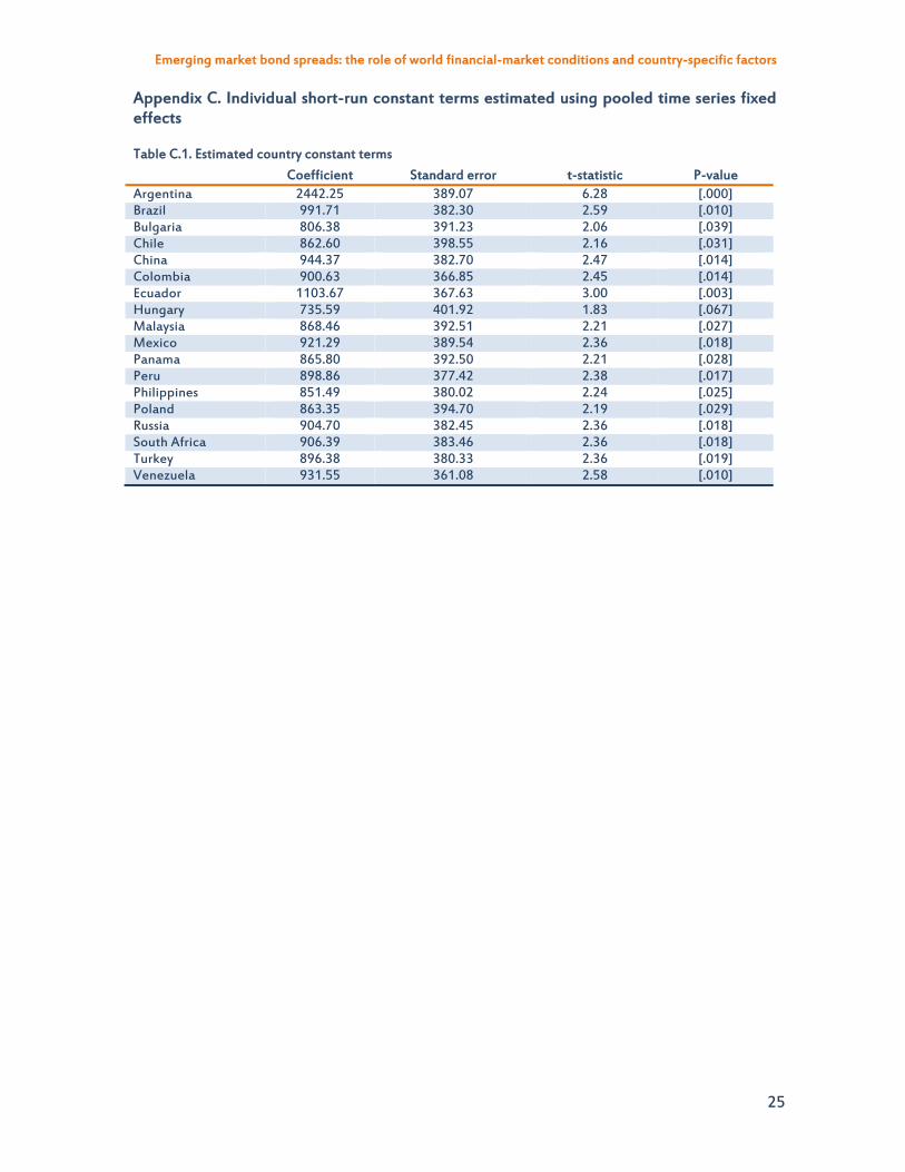
Appendix C. Individual short-run constant terms estimated using pooled time series fixed effects
Table C.1. Estimated country constant terms
Coefficient Standard error t-statistic P-value Argentina 2442.25 389.07 6.28 [.000] Brazil 991.71 382.30 2.59 [.010] Bulgaria 806.38 391.23 2.06 [.039] Chile 862.60 398.55 2.16 [.031] China 944.37 382.70 2.47 [.014] Colombia 900.63 366.85 2.45 [.014] Ecuador 1103.67 367.63 3.00 [.003] Hungary 735.59 401.92 1.83 [.067] Malaysia 868.46 392.51 2.21 [.027] Mexico 921.29 389.54 2.36 [.018] Panama 865.80 392.50 2.21 [.028] Peru 898.86 377.42 2.38 [.017] Philippines 851.49 380.02 2.24 [.025] Poland 863.35 394.70 2.19 [.029] Russia 904.70 382.45 2.36 [.018] South Africa 906.39 383.46 2.36 [.018] Turkey 896.38 380.33 2.36 [.019] Venezuela 931.55 361.08 2.58 [.010]
Emerging market bond spreads: the role of world financial-market conditions and country-specific factors
26
Appendix D. Actual versus predicted EMBI+ spreads
To facilitate comparisons, the range for all countries, except Argentina, Ecuador and Venezuela, is 1000 basis points in units of 100 basis points. Table D.1 (at the end) shows RMSE as well as sample standard deviations and means of EMBI+ spreads. The RMSEs of the model is less than the standard deviations of EMBI+ spreads, except for China and Malaysia.
Note: Brazil’s actual EMBI spreads peaked at 2001 basis points in August 2002.
0
2000
4000
6000
8000Argentina (scale different)
ActualPredicted
0
500
1000
1500
2000
2500Brazil
Actual
Predicted
Emerging market bond spreads: the role of world financial-market conditions and country-specific factors
27
0200400600800
1000 BulgariaActualPredicted
-100
100
300
500
700
900Chile
ActualPredicted
-100
100
300
500 China
ActualPredicted
Emerging market bond spreads: the role of world financial-market conditions and country-specific factors
28
Note: Scale same as Venezuela.
0200400600800
10001200 Columbia
ActualPredicted
010002000300040005000 Ecuador (scale different)
ActualPredicted
-200
0
200
400
600
800 Hungary
ActualPredicted
Emerging market bond spreads: the role of world financial-market conditions and country-specific factors
29
-100
100
300
500
700
900 Malaysia
Actual
Predicted
0200400600800
1000 Mexico
Actual
Predicted
0200400600800
1000 Panama
ActualPredicted
Emerging market bond spreads: the role of world financial-market conditions and country-specific factors
30
0
200
400
600
800
1000Peru
Actual
Predicted
100
300
500
700
900
1100 Philippines
ActualPredicted
0200400600800
1000 Poland
ActualPredicted
Emerging market bond spreads: the role of world financial-market conditions and country-specific factors
31
0200400600800
1000 Russia
ActualPredicted
0
200
400
600
800
1000 South Africa
ActualPredicted
0200400600800
10001200 Turkey
ActualPredicted
Emerging market bond spreads: the role of world financial-market conditions and country-specific factors
32
Note: same scale as Ecuador.
-500
500
1500
2500
3500
4500 Venezuela (scale diffferent)
Actual
Predicted
Emerging market bond spreads: the role of world financial-market conditions and country-specific factors
33
Table D.1 Statistics on predicted and actual EMBI+ spreads
RMSE Standard deviations of actual
EMBI+ Means of actual EMBI+
Argentina 409.28 655.29* 2810.58 Brazil 328.03 440.28 536.87 Bulgaria 85.38 154.26 207.14 Chile 46.98 76.23 132.72 China 74.61 44.61 87.21 Colombia 96.27 187.32 372.46 Ecuador 460.60 866.03 1130.27 Hungary 108.28 128.29 107.67 Malaysia 88.04 77.74 141.78 Mexico 61.29 91.71 217.19 Panama 54.70 110.51 295.12 Peru 86.42 161.25 317.70 Philippines 87.40 117.59 359.65 Poland 53.83 78.61 112.35 Russia 80.24 181.61 283.36 South Africa 94.32 123.57 188.74 Turkey 136.68 204.62 401.31 Venezuela 198.01 426.53 702.36
* The weighted average over two periods January 2002 to June 2005, and June 2005 to July 2009 so as to exclude the large drop in that month. Weights were 0.45 and 0.55.
Emerging market bond spreads: the role of world financial-market conditions and country-specific factors
34
Appendix E. Details on simulated decreases and increases in EMBI+ spreads
Table E.1 Contributions of determinants to declines in EMBI+ spreads (Oct ’02 to Jul ’07, in percentage points – bolded numbers are basis point contributions)