__________________________________________________________________ CREDIT Research Paper

No. 10/03 _____________________________________________________________________

Protection and the Determinants of Household Income in Tanzania 1991-2007

by

Vincent Leyaro and Oliver Morrissey Abstract

This paper analyses the association between household characteristics – in particular size and location, and for the household head age, sector of employment (and the tariff applicable to that sector) and education - and household income using data from the Tanzania Household Budget Survey for the years 1991/92, 2000/01 and 2007. The static analysis of the determinants of household income is based on the full sample and is complemented by a dynamic analysis using a pseudo-panel (representative households). Larger households have lower income; living in urban areas is associated with income around one quarter higher than rural households; and location in the Coastal zone, which includes Dar es Salaam, increases household income by about 15% compared to the poorest region (Central). Years of education of the household head is associated with higher income: each additional year of education adds about 4.5%. Average incomes of agriculture households are lower than for manufacturing households, but within each broad sector incomes appear to be higher in sub-sectors with higher tariffs. Household income tends to increase in both tariffs and education, but the effect of tariffs diminishes or becomes negative for household heads with secondary education and alters over time. Observing that tariffs offer less protection to the incomes of more educated workers compared to less educated (less skilled) workers is consistent with better educated workers being more productive and therefore in firms, or sectors, better able to compete with imports. Given data limitations it would be incorrect to infer a causal effect of tariffs on household incomes. Nevertheless, the analysis is informative about the effect of the cross-sector pattern of tariff protection on household incomes allowing for other determinants.

JEL Classification: D10, H31, O55

Keywords: Household Income, Sector Tariffs, Education, Tanzania

_____________________________________________________________________ Centre for Research in Economic Development and International Trade, University of Nottingham

_____________________________________________________________________ CREDIT Research Paper

No. 10/03

Protection and the Determinants of Household Income in Tanzania 1991-2007

by

Vincent Leyaro and Oliver Morrissey

Outline

1. Introduction

2. Empirical Model and Methods

3. Data Description and Discussion

4. Econometric Results

5. Conclusions and Discussion

References

Appendices

The Authors

Vincent Leyaro is a Lecturer in the Department of Economics, University of Dar-es-Salaam. Oliver Morrissey is Professor in Development Economics and Director of CREDIT, School of Economics, University of Nottingham.

Corresponding Author: oliver.morrissey@nottingham.ac.uk.

Acknowledgements

Useful comments on an earlier version were provided by Simon Appleton. _____________________________________________________________________ Research Papers at www.nottingham.ac.uk/economics/credit/

1

1 Introduction

The prediction that changes in exposure to international trade alter the demand for

and returns to factors and the distribution of incomes within a country is one of the

accepted tenets of trade theory. In developing countries, where the majority of the

population are employed in the informal or household self-employment (business or

farm) sectors and devote a substantial amount of time to production for own

consumption (Winters, 2002), effects on labour demand and income earning

opportunities rather than on relative wages are likely to be the mechanism through

which trade affects income distribution and poverty. This is captured in the Stolper-

Samuelson theorem, which in its simplest form suggests that trade liberalisation

should help the less skilled (the relatively if not absolutely poor), the relatively

abundant factor in developing countries, by increasing demand for the products they

produce thereby raising their incomes. According to this framework, the poor can

gain more from trade openness as it decreases income inequalities. Krueger (1983)

and Bhagwati and Srinivasan (2002) argue that, as developing countries are likely to

have a comparative advantage in goods made with unskilled labour, tariff reduction

should be pro-poor as it raises the wages of unskilled labour in poor (unskilled-labour

abundant) countries. Thus, expanding trade opportunities should cut poverty and

reduce inequality within poor countries.

According to the comprehensive review by Goldberg and Pavcnik (2007)

on the distribution effects of globalization in developing countries, there is no direct

evidence on Stolper-Samuelson (SS) effects; evidence suggests that the unskilled in

developing countries are generally not better off following more than two decades of

trade liberalisation. Distributional change has gone in an opposite direction from that

suggested by conventional wisdom, i.e. even in developing countries, the skilled have

benefitted more than the unskilled. Faced with this puzzling result, various

researchers have challenged the Heckscher-Ohlin (HO) theory, which is the basis of

the SS theorem. Researchers have considered various extensions of the HO-SS model

to explain income (wage) inequality by suggesting other mechanisms through which

trade (openness) affects income distribution (Davis and Mishra, 2007; Easterly, 2007;

Prasad et al, 2007; Kraay and Dollar, 2004; Sala-i-Martin, 2002). The key question

2

remains: do tariffs affect household income and are the effects similar across

households?

The paper addresses this question for Tanzania, employing three waves of

household survey data and applying a pseudo panel technique from repeated cross-

sections (RCS) to econometrically estimate the effects of trade barriers (tariffs) and

tariff reductions on household income in the 1990s and 2000s. Although the method

does not yield precise estimates, as it is not possible to clearly identify the effect of

tariffs on household income and tariff changes are not a treatment effect (there is no

untreated control group), it does permit an informative analysis of the relationship

between household income and household characteristics that may be affected (albeit

indirectly) by trade policy. Tanzania is a relevant case study as it is a low income

country, with around 45 per cent of the population below the poverty line in the early

1990s, with three rounds of survey data spanning 1991 to 2007 during which the trade

regime was reformed.1

The cross-sector tariff reductions that occurred during the period are

exploited to establish a link between trade policy and household income. Average

sector tariffs have fallen from a maximum of 50 per cent in 1991 to 25 per cent in

2000 and 12.5 per cent in 2007 (see Appendix Table A1). Sector average tariffs (at

two digit HS code level) are matched to household data by allocating to a household

the tariff corresponding to the principal sector of employment of the household head.

As the three survey waves do not constitute a panel, the repeated cross-section data is

exploited to form a pseudo panel to track a variety of ‘representative’ households.

While there has been substantial work on incomes (and inequality) and descriptive

analysis of the characteristics of the poor and changes over time (National Bureau of

Statistics, 2002 and 2008; Treichel, 2005), to our knowledge there is no multivariate

econometric analysis of the effects of tariffs on household income (measured as

consumption expenditure, earnings or wages) in Tanzania.

The empirical literature on the effects of trade policy change on incomes

can be categorised into two broad approaches, cross country studies (typically ex post

1 Identifying the effects of trade is confounded as many other reforms were implemented in addition to tariff reductions: price decontrol; rationalization of tariffs and taxes; dismantling of import restrictions (non-tariff barriers); devaluation of the local currency, introducing a market-determined exchange rate and incentives to promote exports; reform of fiscal and monetary policies.

3

econometric analysis) and country case studies (usually ex ante simulation).2 Most

cross-country studies are based on aggregate (macro) data and are limited: problems

of data quality; difficulty of distinguishing the effects of trade reforms from other

contemporaneous effects and policy changes; and aggregate data do not capture

distributional effects. Even if researchers attempt to test for the direct effect of trade

on income distribution in aggregate data, there may be significant underlying

heterogeneity (Harrison, 2006; Ravallion, 2004). The case studies focus exclusively

on the experiences of particular developing countries, often ‘predicting’ or simulating

the likely effects using techniques such as computable general equilibrium (CGE)

models (e.g., Hertel and Jeffrey, 2004). Although they can be linked to household

data for microsimulation of distribution effects, CGE models have been criticised for

using very restrictive assumptions (Kirkpatrick and Scrieciu 2007).

To address limitations of these approaches, researchers have called for the

use of micro (highly disaggregated) data, such as at the level of the household or firm,

to identify the impact of trade (liberalization) on income (distribution). Micro level

data studies are able to allow for (household) heterogeneity, although there are

difficulties in addressing endogeneity (even if panel data are available) and

disentangling the effects of trade reforms from other contemporaneous policies.

Despite the increasing availability of survey data in developing countries, there are

few studies examining the effects of trade (policy) on household income (welfare),

especially for Africa.3 To fill this gap, this paper is in the ‘micro data’ tradition and

focuses on the income effect channel.

The remainder of this paper is organized as follows. Section 2 describes

the empirical strategy employed in the context of the literature. The data sources and

variables are discussed in Section 3, which provides a descriptive analysis. Section 4

presents and discusses the empirical estimates. A concluding discussion is provided

in Section 5.

2 See Goldberg and Pavcnik (2007), McCullogh et al (2002), Harrison (2006), Reimer (2002), Winters (2002) and Winters et al (2004). 3 Studies include Ackah et al (2007), Barraud and Calfat (2008), Deaton (1989), Edmonds and Pavcnik (2002), Friedman and Levinsohn (2002), Nicita (2004), Porto (2006), Seshan (2005) and Topalova (2004).

4

2 Empirical Model and Methods

Going beyond the predictions of the SS theorem and macro-based analysis to micro

level analysis that allows for heterogeneity is important in understanding the

mechanisms through which trade affects earnings of households in low income

countries.4 The effect of trade on incomes of the poor (or poverty) has received less

attention than effects on labour (wage) income, and the literature on wage effects is

mostly on middle income countries in Asia and Latin America (Goldberg and

Pavcnik, 2007). Winters et al. (2004) note that trade affects poverty directly through

changes in relative prices faced by households as consumers and producers, the

market for labour (i.e. employment and wage adjustments) and public spending (as

influenced by changes in government revenue). The analysis here only considers the

first of these. To estimate the overall impact of trade reforms on household welfare

requires assessing the effects of trade reforms on prices, and then the effects of price

changes on household welfare. The welfare impacts of changes in the consumer

prices of traded and non-traded goods are called consumption effects, as analysed in

Leyaro et al (2010). This paper concentrates on effects on household earnings, the

income effects, especially labour income for workers with different levels of

education (a proxy for skill differences).

In addition to consumption and income effects, there are other effects as

increased incomes generate demand for services and non-traded goods (McCulloch et

al 2002). These spillover effects are difficult to estimate in partial equilibrium and

only a few studies have adopted this approach, such as Nicita (2004) for Mexico,

Seshan (2005) for Vietnam, Porto (2006) for Argentina. Unlike these studies, the

empirical method used in this study is the reduced form specification where the

relationship between various household characteristics and household income are

examined. We investigate the association of household incomes with tariffs (for the

sector in which the household head is employed) and household characteristics, in

particular sector of employment and level of education of the household head. To the

4 The basic intuition behind the SS theorem applied to labour markets is that an increase in the price of a commodity increases the demand for, and hence returns to, the factors used intensively in production. For example an increase in the prices of labour intensive products will increase wage rate. However, the impact on wages is constrained in developing country with surplus labour (underemployment). As surplus labour is a feature of rural areas and informal sectors it is important to consider other sources of income and employment opportunities in addition to wage income.

5

extent that education is an indication of skills, this allows us to consider the

differential effects of tariff changes on skilled and unskilled labour.

Panel data, where the same households are followed in successive

surveys, facilitates estimation of parameters capturing the dynamic relationship in a

linear dynamic model given as:

itititit xww εβα +′+= −1 (1)

for i = 1, …, N households (denoting the cross-section dimension) over t = 1, … , T

time periods (denoting the time series dimension), where itw is an endogenous

variable of interest, itx′ is a vector of exogenous explanatory variables (including age,

age squared, household size, education, and location variables), α and β are

unknown parameters to be estimated. The error term has the usual error components

structure:

itiit vf +=ε (2)

where itv is idiosyncratic error term with zero mean and assumed to be uncorrelated

over time, and if represents a fixed effect. If panel data are available one can

estimate α and β using GMM estimators by first differencing (1) and then using

lagged values of 1−itw as instruments.

Suitable data are not available for Tanzania as the household surveys do

not have a panel dimension, i.e. different households are surveyed in each wave.

Following the seminal work by Deaton (1985) and extensions, one can exploit the

repeated cross-section (RCS) data to form a pseudo-panel to group (or aggregate) the

individual observations into cohorts comprising households with some similar

observed time invariant characteristic(s), such as location or year of birth and sex of

household head. Estimating parameters from pseudo panels has spawned a literature.

To capture the dynamics, Moffit (1993), Collado (1998), Girma (2000) and

McKenzie (2004) predict the lagged dependent variable from an auxiliary regression

and use this to estimate the dynamic model. Verbeek and Vella (2005) criticized these

estimators where the lagged dependent variable is replaced by a predicted value as

inconsistent unless strong, and often unrealistic, conditions are imposed on the

6

exogenous variables. They proposed that inconsistent results can be overcome by

instrumenting other explanatory variables using the standard within estimator applied

to a dynamic model in terms of cohort averages rather than individual observations.

We consider these issues in our estimation.

We exploit the availability of three rounds of household surveys in

Tanzania to construct a pseudo panel and track household cohorts through the three

cross-sections. Cohorts are constructed by grouping households based on three

characteristics: age of head, gender of head and region in which the household is

located. As there are only two values for gender (male or female) and 20 regions, the

discretion relates to the span for age of household head. To capture the working

population we consider only households with heads between the ages of 18 and 62

initially. As the three surveys are nine and seven years apart, for the first cross-

section (1991/92) the sample only includes households whose heads are aged 18 to

62, the second cross-section (2000/01) only includes households with heads aged 27

to 72 (i.e. adding nine years) and the third cross-section (2007) only includes

households whose heads are aged 34 to 78 (adding seven years). Thus, most heads of

household are in the normal working age span in all surveys and households ‘age’

over time. We use 5-year bands in defining the generational cohorts resulting in nine

birth cohorts; for example, the first age cohort studied was aged 18-22 in 1991/92,

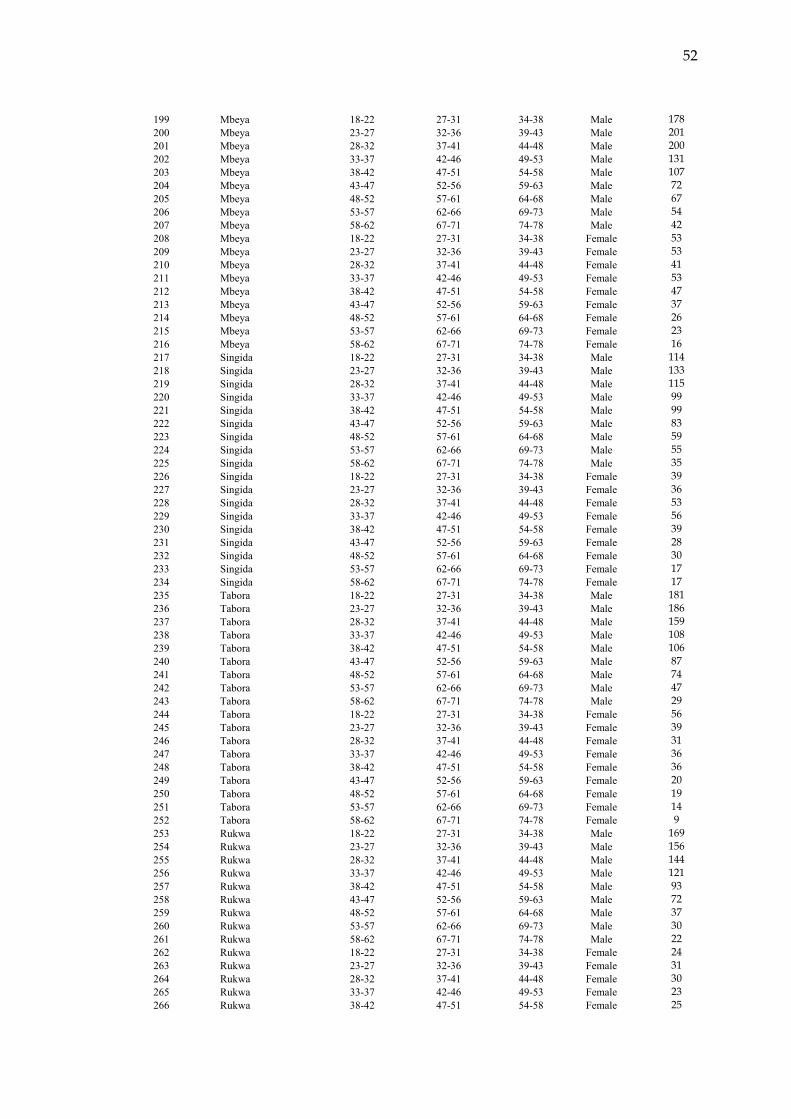
27-31 in 2000/1 and 34-38 in 2007. This gives 360 (9 age x 2 gender x 20 regions)

‘representative households’ in the pseudo panel (see Appendix Table A12); Ackah et

al (2007), apply a similar approach to Ghana.

There is a trade-off between the size and number of ‘representative

households’ or cohorts (e.g. male heads of a particular age in Dar-es-Salaam): if the

cohort cells contain a large number of households, the number of cohorts (the cross-

section dimension of the pseudo-panel) will be small. On the other hand, if we aim

for a large cross-section dimension (some of) the cohorts may contain relatively few

households (and hence may not be representative of the ‘household type’). In fact

many of our 360 ‘representative household’ cohorts are quite small; about 25% of the

cells, mostly female-headed cohorts in rural locations, comprise 30 or fewer

households (Appendix Table A12). On the other hand, as there are three waves of the

survey we have a total of 1080 observations in the pseudo-panel, and even using

7

lagged income the sample size is 720. Thus, even for the pseudo-panel the sample is

reasonably large (although we do lose a number of cells than have no households in

one of the three surveys).

Given the large proportion of cells of small size, the pseudo-panel may

not provide robust estimates and we only use it to complement the analysis using data

on all households (although when we want to allow for lagged income, the pseudo-

panel is our only option). For consistency, we estimate a ‘cohort panel’ when using

all the households, i.e. for each survey, the households are allocated to the relevant

cohort (of the 360) and the data are organized by these cohorts which are tracked over

the surveys. Thus, although we do not have a panel of the same households, we have

a panel of cohorts of similar households according to the stated criteria (age of head,

gender of head and region in which the household is located). Results are reported for

both the cohort and pseudo panel where both can be used. We also estimated the

models by simply pooling the households and some of these results are reported for

comparison.

After matching each household with the relevant sector tariff (i.e. the

tariff for the sector in which the head gets the majority of income), we examine how

household income (or welfare, measured as real expenditure) relates to trade reforms

(as captured by tariffs). The approach is based on modelling the natural logarithm of

per adult equivalent consumption expenditure of households, adjusted for variations

in prices between localities and over time (using the Fisher index as in Leyaro et al,

2010). Household welfare ( w , i.e. real per adult expenditure) is specified as:

21 2 3 4 5

6 1

ln it it it it it i

i jt it

w age age hsize educ urbanecoz tariff

α β β β β ββ δ μ

= + + + + ++ + + (3)

Subscripts i and t index households and survey years respectively: age is the age of

household head at the time of the survey, 2age is squared age, hsize is the size of the

household, educ is education of the household head, urban is a 0/1 dummy (1 for

households in urban localities and zero otherwise), ecoz is four climatic zones

8

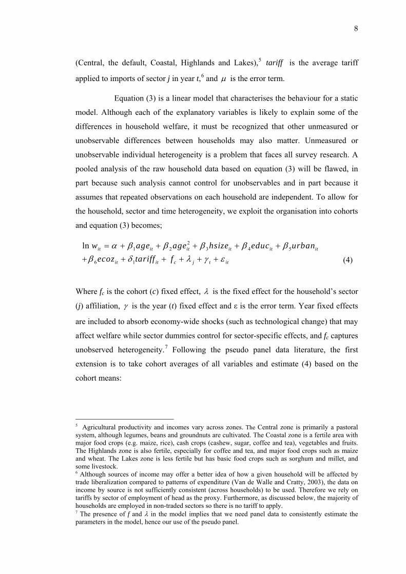
(Central, the default, Coastal, Highlands and Lakes),5 tariff is the average tariff

applied to imports of sector j in year t,6 and μ is the error term.

Equation (3) is a linear model that characterises the behaviour for a static

model. Although each of the explanatory variables is likely to explain some of the

differences in household welfare, it must be recognized that other unmeasured or

unobservable differences between households may also matter. Unmeasured or

unobservable individual heterogeneity is a problem that faces all survey research. A

pooled analysis of the raw household data based on equation (3) will be flawed, in

part because such analysis cannot control for unobservables and in part because it

assumes that repeated observations on each household are independent. To allow for

the household, sector and time heterogeneity, we exploit the organisation into cohorts

and equation (3) becomes;

21 2 3 4 5

6 1

ln it it it it it it

it it c j t it

w age age hsize educ urbanecoz tariff f

α β β β β ββ δ λ γ ε

= + + + + ++ + + + + + (4)

Where fc is the cohort (c) fixed effect, λ is the fixed effect for the household’s sector

(j) affiliation, γ is the year (t) fixed effect and ε is the error term. Year fixed effects

are included to absorb economy-wide shocks (such as technological change) that may

affect welfare while sector dummies control for sector-specific effects, and fc captures

unobserved heterogeneity.7 Following the pseudo panel data literature, the first

extension is to take cohort averages of all variables and estimate (4) based on the

cohort means:

5 Agricultural productivity and incomes vary across zones. The Central zone is primarily a pastoral system, although legumes, beans and groundnuts are cultivated. The Coastal zone is a fertile area with major food crops (e.g. maize, rice), cash crops (cashew, sugar, coffee and tea), vegetables and fruits. The Highlands zone is also fertile, especially for coffee and tea, and major food crops such as maize and wheat. The Lakes zone is less fertile but has basic food crops such as sorghum and millet, and some livestock. 6 Although sources of income may offer a better idea of how a given household will be affected by trade liberalization compared to patterns of expenditure (Van de Walle and Cratty, 2003), the data on income by source is not sufficiently consistent (across households) to be used. Therefore we rely on tariffs by sector of employment of head as the proxy. Furthermore, as discussed below, the majority of households are employed in non-traded sectors so there is no tariff to apply. 7 The presence of f and λ in the model implies that we need panel data to consistently estimate the parameters in the model, hence our use of the pseudo panel.

9

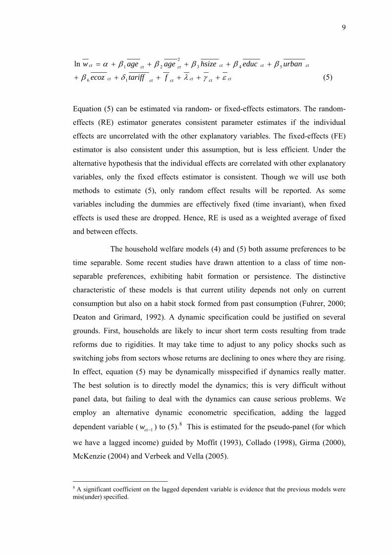
ctctctctctct

ctctctctctct

ftariffecoz

urbaneduchsizeageagew

εγλδβ

βββββα

++++++

+++++=

16

5432

21ln

(5)

Equation (5) can be estimated via random- or fixed-effects estimators. The random-

effects (RE) estimator generates consistent parameter estimates if the individual

effects are uncorrelated with the other explanatory variables. The fixed-effects (FE)

estimator is also consistent under this assumption, but is less efficient. Under the

alternative hypothesis that the individual effects are correlated with other explanatory

variables, only the fixed effects estimator is consistent. Though we will use both

methods to estimate (5), only random effect results will be reported. As some

variables including the dummies are effectively fixed (time invariant), when fixed

effects is used these are dropped. Hence, RE is used as a weighted average of fixed

and between effects.

The household welfare models (4) and (5) both assume preferences to be

time separable. Some recent studies have drawn attention to a class of time non-

separable preferences, exhibiting habit formation or persistence. The distinctive

characteristic of these models is that current utility depends not only on current

consumption but also on a habit stock formed from past consumption (Fuhrer, 2000;

Deaton and Grimard, 1992). A dynamic specification could be justified on several

grounds. First, households are likely to incur short term costs resulting from trade

reforms due to rigidities. It may take time to adjust to any policy shocks such as

switching jobs from sectors whose returns are declining to ones where they are rising.

In effect, equation (5) may be dynamically misspecified if dynamics really matter.

The best solution is to directly model the dynamics; this is very difficult without

panel data, but failing to deal with the dynamics can cause serious problems. We

employ an alternative dynamic econometric specification, adding the lagged

dependent variable ( 1ctw − ) to (5).8 This is estimated for the pseudo-panel (for which

we have a lagged income) guided by Moffit (1993), Collado (1998), Girma (2000),

McKenzie (2004) and Verbeek and Vella (2005).

8 A significant coefficient on the lagged dependent variable is evidence that the previous models were mis(under) specified.

10

Equation (5) imposes a uniform and linear restriction on the parameter 1δ

(and also in the linear dynamic model), the effect of tariff on welfare. The implicit

assumption that all households would experience the same effects from tariffs is

unlikely. Equation (6) introduces interaction terms to explicitly allow the effect of

tariffs on households to differ. We hypothesize that differences can, at least partially,

be attributed to different education qualifications and sector of employment of the

household head. Equation (4) becomes (with similar addition to the dynamic

specification in (5)):

21 2 3 4 5 6

1 2 2

ln it it it it it it it

jt it it it it j t it

w age age hsize educ urban ecoztariff tariff educ tariff sctr

α β β β β β βδ δ δ λ γ ε

= + + + + + ++ + ∗ + ∗ + + + (6)

where educ is three mutually exclusive educational dummies (primary, secondary and

tertiary) denoting the education qualification category of the household head where

‘no education’ is the omitted category. Primary is where the household head has at

least primary or below primary, including adult education (i.e. better than no

education); secondary is household heads with secondary or post-secondary

education; and tertiary is household heads with graduate level education. The sctr

dummies for the thirteen traded sectors of household head employment (listed in

Table A1) are interacted with tariffs. Households employed in non-traded sectors are

assumed to face a zero tariff, so any effects of tariffs can be interpreted relative to

such households.9

The mediating variable (household head years of education) is

transformed by mean centring to create new scales, i.e. by subtracting the sample

mean of household head years of education from the value for each household, to

give deviation from the mean. We estimate the product term of (6) with the

transformed variables such that our coefficient of interest 1δ can be interpreted as the

predicted effect of tariff on income when education is at the sample mean for

primary, secondary or tertiary education. This is the marginal impact of tariff on

9 Topalova (2004:16) argued that all households employed in non-tradable sectors should be assigned a tariff of zero as there are no imports to tax. One could argue for an infinite tariff; as there are no imports there is no competition from imports hence no downward pressure on domestic prices that a tariff could offset. It is not obvious how to incorporate an infinite tariff, and the zero tariff implies only that tariff interaction terms are omitted for these households (other characteristics are included).

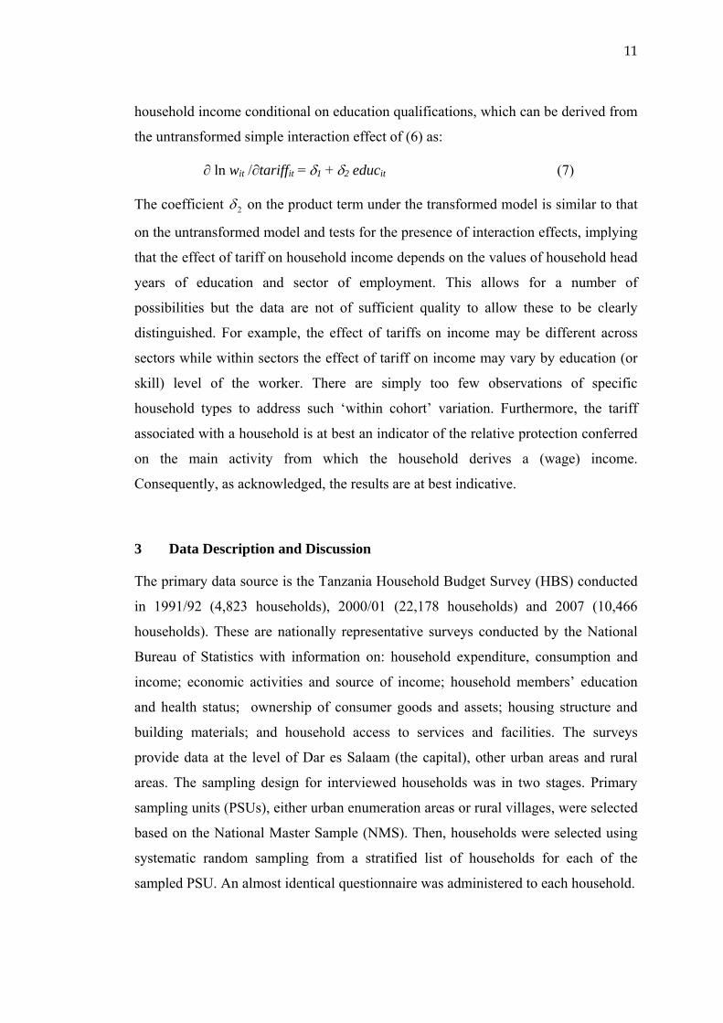
11

household income conditional on education qualifications, which can be derived from

the untransformed simple interaction effect of (6) as:

∂ ln wit /∂tariffit = δ1 + δ2 educit (7)

The coefficient 2δ on the product term under the transformed model is similar to that

on the untransformed model and tests for the presence of interaction effects, implying

that the effect of tariff on household income depends on the values of household head

years of education and sector of employment. This allows for a number of

possibilities but the data are not of sufficient quality to allow these to be clearly

distinguished. For example, the effect of tariffs on income may be different across

sectors while within sectors the effect of tariff on income may vary by education (or

skill) level of the worker. There are simply too few observations of specific

household types to address such ‘within cohort’ variation. Furthermore, the tariff

associated with a household is at best an indicator of the relative protection conferred

on the main activity from which the household derives a (wage) income.

Consequently, as acknowledged, the results are at best indicative.

3 Data Description and Discussion

The primary data source is the Tanzania Household Budget Survey (HBS) conducted

in 1991/92 (4,823 households), 2000/01 (22,178 households) and 2007 (10,466

households). These are nationally representative surveys conducted by the National

Bureau of Statistics with information on: household expenditure, consumption and

income; economic activities and source of income; household members’ education

and health status; ownership of consumer goods and assets; housing structure and

building materials; and household access to services and facilities. The surveys

provide data at the level of Dar es Salaam (the capital), other urban areas and rural

areas. The sampling design for interviewed households was in two stages. Primary

sampling units (PSUs), either urban enumeration areas or rural villages, were selected

based on the National Master Sample (NMS). Then, households were selected using

systematic random sampling from a stratified list of households for each of the

sampled PSU. An almost identical questionnaire was administered to each household.

12

The tariff data is aggregated to the two digit Harmonized System (HS)

level for the survey years using both ad valorem scheduled (published MFN) and

implicit (collected import duty relative to CIF import value) tariffs from the Tanzania

Revenue Authority, Customs Department. Given the matching of tariffs at the two

digit HS level we have 19 sectors, 13 are in the traded goods sector and six in the

non-traded sector. The sample is selected conditional on household head working

(and so having a main source of income) and aged between 18 and 78 years; any

other households are excluded. Each selected household is mapped to the sector of

either main employment or source of income of the household head. This leaves a

sample of 4,262 in 1991/92, 18,241 in 2000/01 and 6,534 in 2007.

Table 1 Summary Statistics on Household Characteristics

Variable

1991/92 2000/01 2007

Mean Std. Dev. Mean Std. Dev. Mean Std. Dev.

Welfare (Tshs) 12,393 10,081 13,024 10,692 14,351 13,410

Log Welfare 9.19 0.68 9.25 0.66 9.32 0.68

Age Head 39.91 10.96 42.96 12.10 49.89 11.36

AgeHead2 1,7123 911 1,993 1,133 2,618 1,213

Hh Size 5.72 3.52 5.09 3.04 5.27 3.08

Years Education 5.91 4.96 10.88 0.41 11.32 7.23

No Education (%) 0.22 0.41 0.22 7.04 0.26 0.44

Basic (%) 0.70 0.46 0.68 0.42 0.64 0.48

Secondary (%) 0.05 0.22 0.06 0.47 0.06 0.23

Post Secondary (%) 0.01 0.11 0.02 0.24 0.02 0.14

Tertiary (%) 0.01 0.11 0.02 0.13 0.02 0.14

1991-2001 2000-2007 1991-2007 Real Welfare Change (%) 5.09 10.18 15.79

Source: Calculated from Tanzania Household Budget Surveys for 1991/92, 2000/01 and 2007. Notes: The reported figures are weighted using survey weights.

This section describes the data on household head main source of income, economic

activities, education and poverty status to illustrate the variation across households

and over time. We start by looking at the key household-level variables specified in

equation (3): a set of demographic variables that relate to linear and quadratic terms

in the age of the head of household to capture possible life cycle effects, educational

attainment and household size. Agro-climatic zones are important for households

13

engaged in agriculture as noted above. Although the skill classification above is based

on three education levels we here consider four: Basic Education (equivalent to

primary); Secondary and Post-Secondary Education (treated separately) and Tertiary

Education.

The summary statics in Table 1 show that there has been a marginal

improvement in almost all of the indicators, particularly education and household

welfare. The categories ‘no education’ and ‘basic education’ account for almost 90

per cent of all heads in each survey, although there has evidently been a gradual

increase over time in years of education and the share of household heads completing

education beyond the primary level.

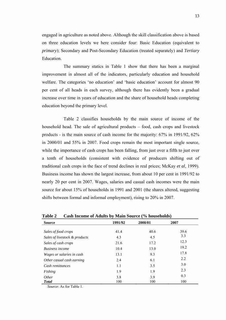
Table 2 classifies households by the main source of income of the

household head. The sale of agricultural products – food, cash crops and livestock

products - is the main source of cash income for the majority: 67% in 1991/92, 62%

in 2000/01 and 55% in 2007. Food crops remain the most important single source,

while the importance of cash crops has been falling, from just over a fifth to just over

a tenth of households (consistent with evidence of producers shifting out of

traditional cash crops in the face of trend declines in real prices; McKay et al, 1999).

Business income has shown the largest increase, from about 10 per cent in 1991/92 to

nearly 20 per cent in 2007. Wages, salaries and casual cash incomes were the main

source for about 15% of households in 1991 and 2001 (the shares altered, suggesting

shifts between formal and informal employment), rising to 20% in 2007.

Table 2 Cash Income of Adults by Main Source (% households) Source 1991/92 2000/01 2007

Sales of food crops 41.4 40.6

39.6 Sales of livestock & products 4.3 4.5 3.3

Sales of cash crops 21.6 17.2 12.3

Business income 10.4 13.0 19.2

Wages or salaries in cash 13.1 9.3 17.8

Other casual cash earning 2.4 6.1 2.2

Cash remittances 1.1 3.5 3.0

Fishing 1.9 1.9 2.3

Other 3.8 3.9 0.3 Total 100 100 100

Source: As for Table 1.

14

In general, there has been a decline in agriculture as a source of income

(mostly due to cash crops) offset by an increasing share of business and employment

income. Although a low share, cash remittances have increased in importance, with a

comparable decline in ‘other’ sources. The latter includes gifts received in cash, cash

from sale of possessions, withdrawal from savings and loans obtained so may be related

to periods of adverse shocks to income. The declining importance of other sources is

consistent with general increases in household welfare.

As shown in Table 1, household income increased only modestly in real

terms: by five per cent between 1991 and 2001, and by 10 per cent between 2001 and

2007 (thus by 15 per cent between 1991 and 2007). However, this is against the

backdrop of large increases in prices of food commodities during the same period

(Leyaro et al 2010). To explore this further we calculate the real change in income for

each source between the survey years using the Fisher index to allow for regional

variations in price changes. The calculations in Table 3 apply the Fisher Index within

periods to give the first and end year constant prices (showing the real change

within the period). For 1991-2001 (and 2001 – 2007), the 1991 (2001) values are

deflated by the relevant Fisher Index to be expressed in 2001 (2007) prices for

comparison with the 2001 (2007) values. For the period 1991 – 2007, there are two

options which yield the same result, either express all incomes in 2001 prices (as in

Table 3) or in 2007 prices.

Table 3 reports changes in household real total expenditure across the

surveys according to the main source of household income. As sales of food crops

are the main income source for the largest number of households (about 40% as

shown in Table 2) this is the main contributor to the modest improvement in average

household income over the period. Real household income from sales of food crops

increased by 5% between 1991 and 2001, by 10% between 2001 and 2007, and thus by

15% over the whole period; this is almost identical to changes in total household

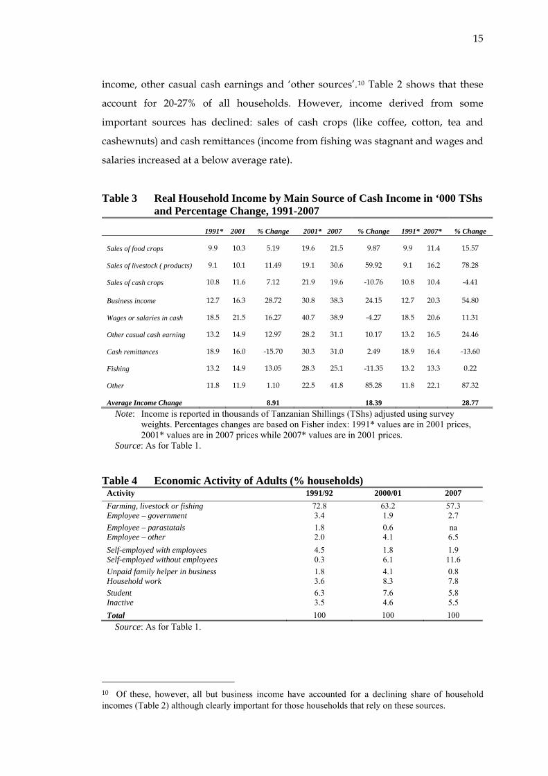
welfare (Table 1). Household income derived from certain sources has seen a much

higher (above average) increase: sales of livestock and livestock products, business

15

income, other casual cash earnings and ‘other sources’.10 Table 2 shows that these

account for 20-27% of all households. However, income derived from some

important sources has declined: sales of cash crops (like coffee, cotton, tea and

cashewnuts) and cash remittances (income from fishing was stagnant and wages and

salaries increased at a below average rate).

Table 3 Real Household Income by Main Source of Cash Income in ‘000 TShs and Percentage Change, 1991-2007

1991* 2001 % Change 2001* 2007 % Change 1991* 2007* % Change Sales of food crops 9.9 10.3 5.19 19.6 21.5 9.87 9.9 11.4 15.57 Sales of livestock ( products) 9.1 10.1 11.49 19.1 30.6 59.92 9.1 16.2 78.28 Sales of cash crops 10.8 11.6 7.12 21.9 19.6 -10.76 10.8 10.4 -4.41 Business income

12.7 16.3 28.72 30.8 38.3 24.15 12.7 20.3 54.80

Wages or salaries in cash 18.5 21.5 16.27 40.7 38.9 -4.27 18.5 20.6 11.31 Other casual cash earning 13.2 14.9 12.97 28.2 31.1 10.17 13.2 16.5 24.46 Cash remittances 18.9 16.0 -15.70 30.3 31.0 2.49 18.9 16.4 -13.60 Fishing 13.2 14.9 13.05 28.3 25.1 -11.35 13.2 13.3 0.22 Other 11.8 11.9 1.10 22.5 41.8 85.28 11.8 22.1 87.32 Average Income Change 8.91 18.39 28.77

Note: Income is reported in thousands of Tanzanian Shillings (TShs) adjusted using survey weights. Percentages changes are based on Fisher index: 1991* values are in 2001 prices, 2001* values are in 2007 prices while 2007* values are in 2001 prices.

Source: As for Table 1.

Table 4 Economic Activity of Adults (% households)

Activity 1991/92 2000/01 2007 Farming, livestock or fishing 72.8 63.2 57.3 Employee – government 3.4 1.9 2.7 Employee – parastatals 1.8 0.6 na Employee – other 2.0 4.1 6.5 Self-employed with employees 4.5 1.8 1.9 Self-employed without employees 0.3 6.1 11.6 Unpaid family helper in business 1.8 4.1 0.8 Household work 3.6 8.3 7.8 Student 6.3 7.6 5.8 Inactive 3.5 4.6 5.5 Total 100 100 100

Source: As for Table 1.

10 Of these, however, all but business income have accounted for a declining share of household incomes (Table 2) although clearly important for those households that rely on these sources.

16

This is consistent with other evidence for Tanzania. Overall (headcount)

poverty declined marginally, from 39 per cent in 1991/92 to 36 per cent in 2000/01

and 33 per cent in 2007. Analysis of the household budget surveys indicates increased

income inequality in Tanzania (National Bureau of Statistics, 2002; 2008), which

explains why poverty has not declined in line with the increase in average incomes.

The growth in incomes from food and livestock products and formal and informal

(casual cash earnings) business may partly be explained by removal of trade barriers

generating increased output of tradables and demand for trade services.

As shown in Table 4, almost two-thirds of the labour force (declining

over 1991-2007) are employed in the agriculture and fisheries sector, and most of

these live outside Dar es Salaam. Informal sector activities such as self employment,

unpaid family business and housewife have been rising, accounting for 20 per cent on

average over the period. Government employment, particularly in parastatals, has

been falling following structural reforms, privatisation and retrenchment. Economic

activities vary by region as well as between urban and rural dwellers. Households in

arid and semi-arid areas are largely involved in grazing (hence sales of livestock

products), those found by larger rivers, lakes or the ocean are involved in fishing,

those found in arable land and valleys are involved in farming, while most people in

urban areas are either employed (government or private sector) or engaged in self

employment or the informal sector. Those classified as unemployed and inactive has

risen from 3.5 per cent in 1991/92 to 5.5 per cent in 2007.

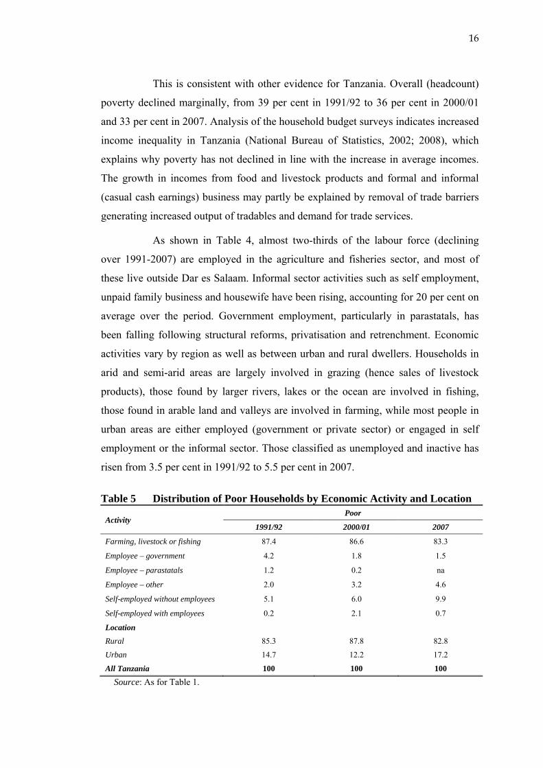
Table 5 Distribution of Poor Households by Economic Activity and Location

Activity Poor

1991/92 2000/01 2007

Farming, livestock or fishing 87.4 86.6 83.3

Employee – government 4.2 1.8 1.5

Employee – parastatals 1.2 0.2 na

Employee – other 2.0 3.2 4.6

Self-employed without employees 5.1 6.0 9.9

Self-employed with employees 0.2 2.1 0.7

Location

Rural 85.3 87.8 82.8

Urban 14.7 12.2 17.2

All Tanzania 100 100 100

Source: As for Table 1.

17

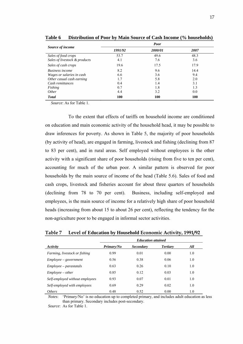
Table 6 Distribution of Poor by Main Source of Cash Income (% households)

Source of income Poor

1991/92 2000/01 2007 Sales of food crops 53.7 49.6 48.3 Sales of livestock & products 4.1 7.6 3.6 Sales of cash crops 19.6 17.5 17.9 Business income 8.2 9.6 14.4 Wages or salaries in cash 6.6 3.6 9.4 Other casual cash earning 1.7 5.8 2.0 Cash remittances 0.4 1.4 3.1 Fishing 0.7 1.8 1.3 Other 4.4 3.2 0.0 Total 100 100 100

Source: As for Table 1.

To the extent that effects of tariffs on household income are conditioned

on education and main economic activity of the household head, it may be possible to

draw inferences for poverty. As shown in Table 5, the majority of poor households

(by activity of head), are engaged in farming, livestock and fishing (declining from 87

to 83 per cent), and in rural areas. Self employed without employees is the other

activity with a significant share of poor households (rising from five to ten per cent),

accounting for much of the urban poor. A similar pattern is observed for poor

households by the main source of income of the head (Table 5.6). Sales of food and

cash crops, livestock and fisheries account for about three quarters of households

(declining from 78 to 70 per cent). Business, including self-employed and

employees, is the main source of income for a relatively high share of poor household

heads (increasing from about 15 to about 26 per cent), reflecting the tendency for the

non-agriculture poor to be engaged in informal sector activities.

Table 7 Level of Education by Household Economic Activity, 1991/92

Activity

Education attained

Primary/No Secondary Tertiary All

Farming, livestock or fishing 0.99 0.01 0.00 1.0

Employee – government 0.56 0.38 0.06 1.0

Employee – parastatals 0.63 0.26 0.10 1.0

Employee – other 0.85 0.12 0.03 1.0

Self-employed without employees 0.93 0.07 0.01 1.0

Self-employed with employees 0.69 0.29 0.02 1.0

Others 0.48 0.52 0.00 1.0 Notes: ‘Primary/No’ is no education up to completed primary, and includes adult education as less

than primary. Secondary includes post-secondary. Source: As for Table 1.

18

Table 8 Level of Education by Household Source of Income, 1991/92

Source of income

Education attained

Primary/No Secondary Tertiary All

Sales of food crops 0.98 0.02 0.00 1.0

Sales of livestock & products 0.96 0.04 0.00 1.0

Sales of cash crops 0.98 0.02 0.00 1.0

Business income 0.92 0.07 0.01 1.0

Wages or salaries in cash 0.63 0.31 0.06 1.0

Other casual cash earning 0.95 0.04 0.01 1.0

Cash remittances 0.95 0.02 0.03 1.0

Fishing 0.99 0.00 0.01 1.0

Other 0.96 0.03 0.00 1.0 Notes: As for Table 7. Source: As for Table 1.

Table 9 Household Poverty Status and Location by Level of Education

Skills/Years Not-Poor Poor Rural Urban

1991/92 Primary/No 0.69 0.31 0.81 0.19 Secondary 0.92 0.08 0.47 0.53 Tertiary 0.95 0.05 0.32 0.68

2000/01 Primary/No 0.71 0.29 0.83 0.17

Secondary 0.91 0.09 0.43 0.57

Tertiary 0.97 0.03 0.41 0.59 2007

Primary/No 0.68 0.32 0.78 0.22 Secondary 0.91 0.09 0.37 0.63 Tertiary 0.93 0.07 0.30 0.70

Notes: As for Table 7. Source: As for Table 1.

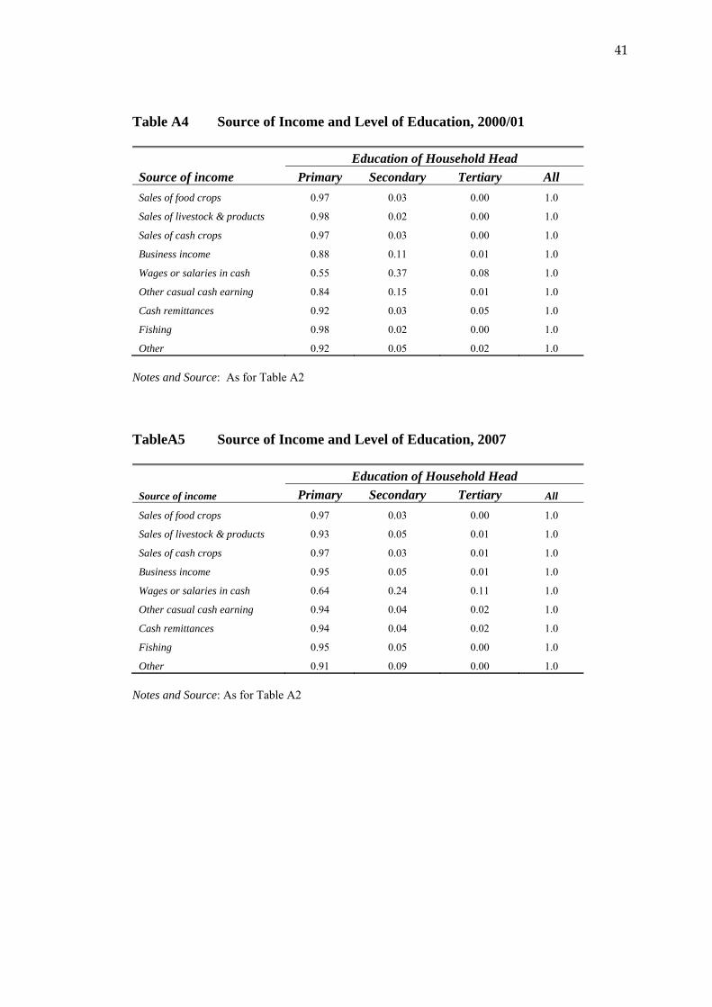
Tables 7 and 8 show the education qualifications (highest educational

level attained) of household heads by economic activity and main source of income

respectively for the 1991/92 survey (see Appendix Tables A2-A5 for the 2000/01 and

2007 surveys respectively). However defined, almost all agriculture households have

only primary education at best (96-99% on different classifications). Education levels

are also very low in the informal sector, whether classified as self-employed without

employees (93% primary in Table 7) or business/casual cash income (92-95%

primary in Table 8). The highest education levels are associated with

19

government/parastatal employment (38%/26% secondary and 6%/10% tertiary in

Table 7), self-employed with employees (29% secondary and 2% tertiary in Table 7),

or wages and salaries (31% secondary and 6% tertiary in Table 8).

Table 9 shows that around 30 per cent of the household heads with no

more than primary education are poor compared and about 80 per cent are in rural

areas. In contrast, only eight per cent of those with secondary and five per cent with

tertiary education are poor, and over 50 and 60 per cent respectively are in urban

areas. In general, household heads with lower education (primary and below) are

most likely to be poor, in rural areas and engaged in farming or other casual

(informal) cash earnings. Household heads with above primary education are most

likely to be in formal sectors, as government or private sector employees or running a

business. As international trade and tariffs will affect sectors in different ways,

especially manufacturing (private sector) and agriculture (with difference between

food and cash crops), these effects may differ by education levels. Consequently, as

effects differ by sector of activity and education, there may be indirect effects on

poverty status.

4 Econometric Results

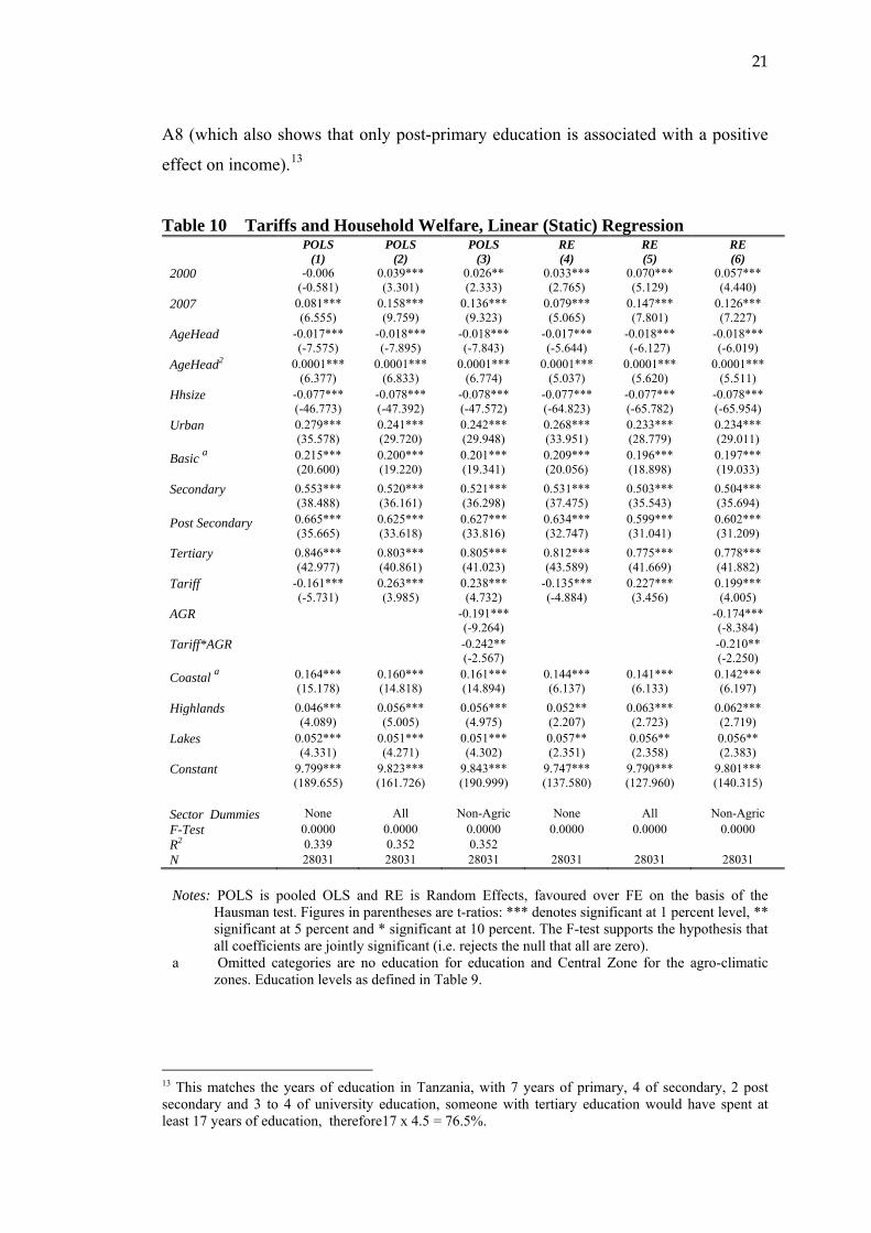
Table 10 reports estimates for the cross-section of all households using pooled OLS

(POLS) based on equation (3) and cohort panel using Random Effects (RE) based on

equation (4).11 The dependent variable is defined as natural logarithm of per adult

equivalent consumption expenditure of the household. Columns 1 and 4 report the

results initially without controlling for sector specific effects; the coefficients on

tariffs are negative and statistically significant in both cases. By assumption non-

traded sector are coded as a zero tariff so incomes in traded sectors appear to be lower

ceteris paribus (as implied by assuming tariffs were infinite in non-traded sectors).

As the coefficient estimates reflect the cross-sector variation in tariffs (relative

protection) they should be interpreted as capturing any association at the sector level

between tariffs and incomes. This implies that sector differences should be allowed

11 Recall that the cohort panel uses all households but organized into the relevant cohorts; although RE and FE yield similar results, RE is preferred due to the inclusion of time invariant explanatory variables in most of our specifications.

20

for, as in the other columns. Note that inferences on the effect of tariff reductions are

not warranted as we cannot identify the effect of tariff changes on income for any

household and have no ‘control group’ for which tariffs did not change.

The results in Columns 2 and 5 allow for unobserved sector heterogeneity

by including sector dummies for the thirteen traded sectors.12 The coefficients on

tariff now have a positive sign and are significant, which suggests that unobserved

sector heterogeneity was responsible for the negative estimate and that within traded

sectors higher tariffs are associated with higher incomes. As agriculture sectors

provide the main income for more than half of households, and average incomes of

agriculture households are lower than for manufacturing households, it might be that

the tariff captures an agriculture effect. To allow for general sector differences we

introduce a dummy AGR = 1 if the head of household is in agriculture and zero

otherwise (manufacturing) in Columns 3 and 6 in Table 10, with tariff*AGR in

addition to tariff. The coefficient on tariff refers to manufactures and remains positive

and significant, but agriculture is that coefficient plus the coefficient on tariff*AGR,

which is negative and significant (but with a much smaller combined coefficient than

on tariff alone). Most other coefficients are largely unaffected in the alternative

specifications.

The effects of protection (the coefficient on tariff), controlling for the

sectors of head main source of income, are positive and statically significant,

implying that higher protection is associated with higher incomes (i.e. incomes are

higher in sectors with higher tariffs, ceteris paribus), except for agriculture compared

to manufacturing as shown in Columns 3 and 6 (but see further discussion below). As

expected from the discussion above, higher education is associated with higher

income. The results in Table 10 indicate that this effect is quite linear: compared to

no education, primary education is associated with a 20% increase in household

income, secondary education around 50%, post-secondary over 60% and tertiary

education with a more than 75% increase in income. This is equivalent to an

increment of 4.5% for each additional year of education as shown in Appendix Table

12 These include (listed in Table A1): food crops; livestock and livestock products; cash crops; fishing; food manufactures; dairy, textile; timber and wood; paper, chemicals; other manufactures; sports goods and building materials. These traded sectors account for about half of the households in the surveys according to recorded sector of employment (Table A1a), suggesting some problems with this variable (informal labour appears to be excluded).

21

A8 (which also shows that only post-primary education is associated with a positive

effect on income).13

Table 10 Tariffs and Household Welfare, Linear (Static) Regression POLS

(1) POLS

(2) POLS

(3) RE (4)

RE (5)

RE (6)

2000

-0.006 (-0.581)

0.039*** (3.301)

0.026** (2.333)

0.033*** (2.765)

0.070*** (5.129)

0.057*** (4.440)

2007

0.081*** (6.555)

0.158*** (9.759)

0.136*** (9.323)

0.079*** (5.065)

0.147*** (7.801)

0.126*** (7.227)

AgeHead

-0.017*** (-7.575)

-0.018*** (-7.895)

-0.018*** (-7.843)

-0.017*** (-5.644)

-0.018*** (-6.127)

-0.018*** (-6.019)

AgeHead2

0.0001***

(6.377) 0.0001***

(6.833) 0.0001***

(6.774) 0.0001***

(5.037) 0.0001***

(5.620) 0.0001***

(5.511) Hhsize

-0.077*** (-46.773)

-0.078*** (-47.392)

-0.078*** (-47.572)

-0.077*** (-64.823)

-0.077*** (-65.782)

-0.078*** (-65.954)

Urban

0.279*** (35.578)

0.241*** (29.720)

0.242*** (29.948)

0.268*** (33.951)

0.233*** (28.779)

0.234*** (29.011)

Basic a

0.215*** (20.600)

0.200*** (19.220)

0.201*** (19.341)

0.209*** (20.056)

0.196*** (18.898)

0.197*** (19.033)

Secondary

0.553*** (38.488)

0.520*** (36.161)

0.521*** (36.298)

0.531*** (37.475)

0.503*** (35.543)

0.504*** (35.694)

Post Secondary

0.665*** (35.665)

0.625*** (33.618)

0.627*** (33.816)

0.634*** (32.747)

0.599*** (31.041)

0.602*** (31.209)

Tertiary

0.846*** (42.977)

0.803*** (40.861)

0.805*** (41.023)

0.812*** (43.589)

0.775*** (41.669)

0.778*** (41.882)

Tariff

-0.161*** (-5.731)

0.263*** (3.985)

0.238*** (4.732)

-0.135*** (-4.884)

0.227*** (3.456)

0.199*** (4.005)

AGR

-0.191*** (-9.264)

-0.174*** (-8.384)

Tariff*AGR

-0.242** (-2.567)

-0.210** (-2.250)

Coastal a

0.164*** (15.178)

0.160*** (14.818)

0.161*** (14.894)

0.144*** (6.137)

0.141*** (6.133)

0.142*** (6.197)

Highlands

0.046*** (4.089)

0.056*** (5.005)

0.056*** (4.975)

0.052** (2.207)

0.063*** (2.723)

0.062*** (2.719)

Lakes

0.052*** (4.331)

0.051*** (4.271)

0.051*** (4.302)

0.057** (2.351)

0.056** (2.358)

0.056** (2.383)

Constant

9.799*** (189.655)

9.823*** (161.726)

9.843*** (190.999)

9.747*** (137.580)

9.790*** (127.960)

9.801*** (140.315)

Sector Dummies

None

All

Non-Agric

None

All

Non-Agric

F-Test 0.0000 0.0000 0.0000 0.0000 0.0000 0.0000 R2 0.339 0.352 0.352 N 28031 28031 28031 28031 28031 28031 Notes: POLS is pooled OLS and RE is Random Effects, favoured over FE on the basis of the

Hausman test. Figures in parentheses are t-ratios: *** denotes significant at 1 percent level, ** significant at 5 percent and * significant at 10 percent. The F-test supports the hypothesis that all coefficients are jointly significant (i.e. rejects the null that all are zero).

a Omitted categories are no education for education and Central Zone for the agro-climatic zones. Education levels as defined in Table 9.

13 This matches the years of education in Tanzania, with 7 years of primary, 4 of secondary, 2 post secondary and 3 to 4 of university education, someone with tertiary education would have spent at least 17 years of education, therefore17 x 4.5 = 76.5%.

22

As commonly observed in the literature, larger households have lower

(per adult equivalent) income (income falls by about 7% for each additional family

member); living in urban areas is associated with higher income (23-28% higher than

rural households). For Tanzania, location in different ecological zones is important

(results are relative to the Central zone, the poorest of the ecological regions and

primarily pastoral). Being in the Coastal zone, which includes Dar es Salaam (the

business capital) but is also a major area for food and cash crop production, increases

household income by about 15% (similar to being in urban areas), whereas being in

either the Highlands (an area for major food grains, and coffee and tea) or Lakes

zones (staple foods and cotton) increases income by around five per cent.

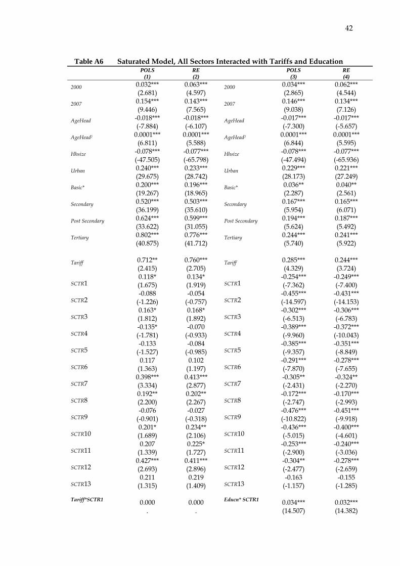
To explore sector-specific effects in more detail we ‘saturated’ the model

with the 13 traded sector dummies and 13 sector*tariff (as well as with 13

sector*education) interaction terms and report all estimates in Appendix Table A6.

Two points are worth emphasizing as we do not want to consider sectors in detail

(although all sector*tariff interaction terms are negative the effect is this combined

with the coefficient on the sector dummy, and just over half of both are significant).

First, the negative tariff*AGR term seems to be attributable to Livestock and

especially (given its importance as a source of income) cash crops (sectors 2 and 3);14

food crop production, the single largest employment sector, emerges as the ‘baseline’.

In general, tariffs are lower (Table A1) and incomes are higher for food producers

within agriculture, which explains the negative coefficient on tariff*AGR in Table 10.

Second, when significant the effect for six manufacturing sectors is also negative: one

is agriculture-related (dairy), textiles and wood (sectors 7 and 8) are among the main

manufacturing sectors, and sectors 11-13 are small in terms of employment.

Appendix Table A7 differentiates between broad agriculture and manufacturing

14 There is an anomaly regarding data on cash crops (sector 3) in the 2000/01 survey as although cash crops appear to be the main source of income for 17% of households (Table 2), only some three per cent of household heads report this as their sector of employment (Table A1b). We are using answers to different questions, one where the head declares their main sector of employment (to match to tariffs) and another giving information on income from different sources (presumably including own production for food). There are a number of possible reasons for a discrepancy, related to the likelihood that households producing cash crops also have other (multiple) sources of income (in particular food crops or off-farm), so they could view these as other sources of employment. Table 3 shows a significant decline in cash crop income so a possibility is that the head engaged in some other activity to earn extra income, although cash crops were still the main source of income (involving other members). We acknowledge this as another limitation of the data (specifically in trying to identify the effect of tariffs).

23

sectors. The results demonstrate that incomes in agriculture households tend to be

lower than for manufacturing households, and overall tariffs tend to be positively

associated with income, but within each broad sector tariffs are negatively associated

with income. In other words, households employed in manufacturing sectors tend to

have higher incomes than households employed in agriculture but within agriculture

incomes are lower in sectors with higher tariffs and similarly within manufacturing.

These leave the result of a positive coefficient on tariff itself something of a mystery,

so we now explore this further. Sector of employment tends to be an important

determinant of income, and one possibility is that it is sectors for which the dummy

and interaction terms are insignificant (the most important of which, in terms of

employment, is manufactured foods, which has relatively high tariffs) account for the

positive coefficient on tariff itself.

The influence of agriculture sectors against other sectors is apparent. As

envisaged, households in agriculture sectors tend to have lower income compared to

those employed in manufacturing. Within agriculture, household incomes tend to be

higher for producers of cash crops (which face the highest tariffs) up to the early

2000s; by the 2007 survey, incomes were higher for households selling food crops

(the lowest tariffs and largest employment share) or livestock products (Table 3).

Thus, the results in Table 10 capture cross-sector effects and how these change over

time. Furthermore, in general tariffs (and incomes) are higher for manufactured

sectors than food crops; this offers an explanation for the finding of a positive

significant coefficient on tariffs. The negative interaction between agriculture and

tariffs may be because tariffs on cash crops remained relatively high while incomes

fell significantly. A similar point may hold within manufacturing, i.e. incomes may

have been higher but fell faster or grew slower in sectors with relatively high tariffs.

As Tanzania has implemented substantial tariff reductions for the past two decades

these distinctions must be considered (and later we estimate a dynamic model): across

sectors tariffs may be positively associated with income but this need not hold over

time. Indeed, there is some tendency for incomes to have risen faster in sectors with

lower tariffs or where tariffs were reduced more. This is a correlation, driven largely

by food crops, so no causal inferences can be drawn. The estimation and analysis in

the rest of the chapter uses dummies to control for sector heterogeneity, especially the

agriculture sector (tariff*AGR).

24

Table 11 Marginal Impacts of Household Head Education on Income, Cohort Panel Static Regression RE

(1) RE (2)

RE (3)

RE (4)

2000

0.048*** (3.760)

0.063*** (4.906)

0.064*** (4.868)

0.062*** (4.667)

2007

0.107*** (6.110)

0.141*** (8.020)

0.136*** (7.609)

0.131*** (7.255)

AgeHead

-0.016*** (-5.516)

-0.017*** (-5.862)

-0.015*** (-4.817)

-0.016*** (-5.363)

AgeHead2

0.000*** (5.754)

0.000*** (4.779)

0.000*** (3.652)

0.000*** (3.945)

Hhsize

-0.078*** (-66.600)

-0.076*** (-64.241)

-0.076*** (-62.633)

-0.076*** (-62.662)

Urban

0.218*** (27.146)

0.255*** (31.528)

0.271*** (32.949)

0.293*** (35.919)

Tariff

0.202*** (4.077)

0.189*** (3.755)

0.612*** (8.769)

0.103** (2.015)

AGR

-0.171*** (-8.287)

-0.191*** (-9.133)

-0.232*** (-10.894)

-0.221*** (-10.350)

Tariff*AGR

-0.226** (-2.427)

-0.183* (-1.936)

-0.099 (-1.625)

-0.166* (-1.726)

Education

0.047*** (49.723)

Educ*Tariff

-0.028*** (-4.840)

Primary

-0.409*** (-40.479)

Primary*Tariff

0.060 (0.848)

Secondary

0.256*** (23.870)

Secondary*Tariff

-0.645*** (-9.311)

Tertiary

0.505*** (27.592)

Tertiary*Tariff

0.097 (0.655)

Coastal*

0.138*** (5.912)

0.149*** (6.487)

0.152*** (6.570)

0.145*** (6.060)

Highlands

0.060** (2.538)

0.077*** (3.356)

0.082*** (3.536)

0.086*** (3.559)

Lakes

0.055** (2.245)

0.065*** (2.728)

0.069*** (2.899)

0.070*** (2.825)

Constant

9.677*** (138.668)

10.360*** (147.088)

9.931*** (140.319)

9.998*** (139.283)

Sector Dummies Non-Agric Non-Agric Non-Agric Non-Agric F-Test 0.0000 0.0000 0.0000 0.0000 N 27976 28031 28031 28031

Notes: As for RE in Table 10; Education is measured as number of years but each level of

education variable is transformed as indicated in text. Estimates with the education variables but without the education*tariff interactions are in Table A8; the signs and significance of other variables are unaltered and the magnitudes are very similar.

25

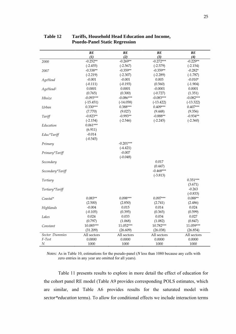
Table 12 Tariffs, Household Head Education and Income, Psuedo-Panel Static Regression

RE (1)

RE (2)

RE (3)

RE (4)

2000

-0.252** (-2.455)

-0.269** (-2.567)

-0.272*** (-2.579)

-0.229** (-2.154)

2007

-0.338** (-2.219)

-0.359** (-2.307)

-0.359** (-2.289)

-0.282* (-1.787)

AgeHead

-0.001 (-0.111)

-0.001 (-0.193)

0.003 (0.560)

-0.010* (-1.904)

AgeHead2

0.0001 (0.765)

0.0001 (0.300)

-0.0001 (-0.727)

0.0001 (1.351)

Hhsize

-0.093*** (-15.451)

-0.086*** (-14.058)

-0.083*** (-13.422)

-0.082*** (-13.322)

Urban

0.330*** (7.770)

0.388*** (9.027)

0.409*** (9.448)

0.407*** (9.356)

Tariff

-0.823** (-2.154)

-0.993** (-2.546)

-0.888** (-2.245)

-0.934** (-2.360)

Education

0.061*** (6.911)

Educ*Tariff

-0.014 (-0.545)

Primary

-0.201*** (-4.421)

Primary*Tariff

-0.007 (-0.048)

Secondary

0.017 (0.447)

Secondary*Tariff

-0.468*** (-3.813)

Tertiary

0.351*** (3.671)

Tertiary*Tariff

-0.263 (-0.833)

Coastal*

0.083** (2.500)

0.098*** (2.850)

0.097*** (2.741)

0.088** (2.486)

Highlands

-0.004 (-0.105)

0.015 (0.395)

0.014 (0.365)

0.024 (0.599)

Lakes

0.024 (0.797)

0.033 (1.068)

0.034 (1.082)

0.027 (0.847)

Constant

10.085*** (31.209)

11.052*** (26.609)

10.782*** (26.038)

11.059*** (26.854)

Sector Dummies All sectors All sectors All sectors All sectors F-Test 0.0000 0.0000 0.0000 0.0000 N 1000 1000 1000 1000

Notes: As in Table 10, estimations for the pseudo-panel (N less than 1080 because any cells with

zero entries in any year are omitted for all years).

Table 11 presents results to explore in more detail the effect of education for

the cohort panel RE model (Table A9 provides corresponding POLS estimates, which

are similar, and Table A6 provides results for the saturated model with

sector*education terms). To allow for conditional effects we include interaction terms

26

for tariffs and household head education (as well as the AGR dummy). As mentioned

above, we transform the education variable so the coefficient on interaction terms can

be interpreted as the marginal impact of tariff on household income for a given level

of education (primary, secondary and tertiary). The coefficient on tariff controlling

for sector effects is positive and significant, as is the coefficient on Education

(measured as number of years), but the coefficient on the interaction term is negative

and statistically significant (Column 1). Household income appears to be increasing

in both tariffs (but not in agriculture) and education, but the effect of tariffs

diminishes, or becomes negative, as level of education increases. That is, the

marginal impact of tariffs on welfare is decreasing in level of education.

Distinguishing the three levels of education shows that those with secondary

education seem not to benefit from higher tariffs. When interaction terms between

tariffs and each level of education are included separately, only the coefficient on

secondary education is statistically significant, and negative (Table 11, Columns 2-4).

In this case, the coefficient on the interaction term almost completely offsets that on

tariffs; tariffs are not associated with higher income conditional on having secondary

education (but having secondary education itself does increase income). There is

likely to be a strong association between agriculture households and households with

no more than primary education, both of which are associated with lower incomes,

whereas household heads with secondary and especially tertiary education are more

likely to be employed in manufacturing sectors (Tables 8, A4. and A5). The negative

association between tariffs and secondary education is likely to apply within

manufacturing. One interpretation is that tariffs tend to protect the incomes of less

educated (less skilled) workers more than for more educated workers, consistent with

observing that import competition presents a greater challenge to the incomes of

relatively less educated (less productive) workers.

27

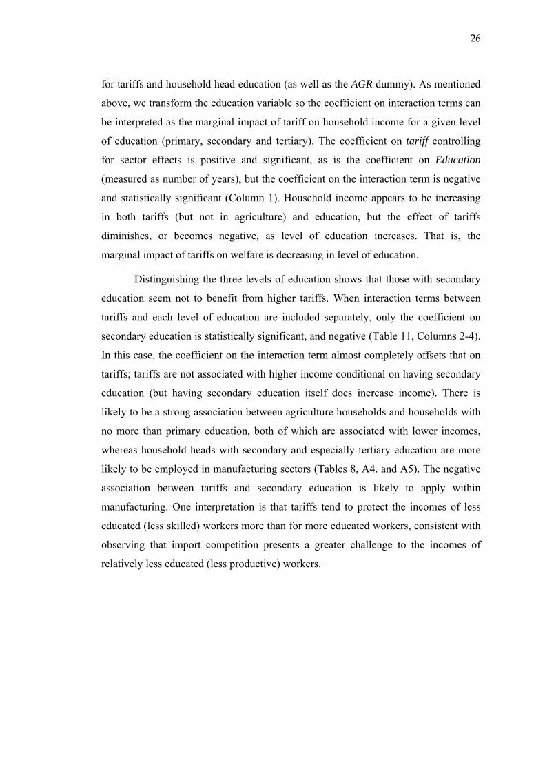
Table 13 Tariffs, Household Head Education and Income, Dynamic Psuedo-Panel Regression

RE (1)

RE (2)

RE (3)

RE (4)

2007

-0.236*** (-2.792)

-0.241*** (-2.755)

-0.253*** (-2.835)

-0.209** (-2.365)

Lag Welfare

0.045 (1.554)

0.056* (1.848)

0.072** (2.365)

0.055* (1.816)

AgeHead

0.009 (1.134)

0.011 (1.273)

0.006 (0.711)

-0.000 (-0.025)

AgeHead2

-0.0001 (-0.701)

-0.0001 (-1.213)

-0.0001 (-0.836)

-0.0001 (-0.290)

Hhsize

-0.099*** (-13.044)

-0.093*** (-11.988)

-0.089*** (-11.265)

-0.084*** (-10.871)

Urban

0.223*** (3.994)

0.293*** (5.188)

0.345*** (6.066)

0.277*** (4.769)

Tariff

-1.981*** (-3.194)

-2.081*** (-3.255)

-2.228*** (-3.414)

-2.083*** (-3.234)

Education

0.057*** (8.970)

Primary

-0.193*** (-6.142)

Secondary

0.104*** (3.318)

Tertiary

0.317*** (5.169)

Coastal*

0.093*** (2.654)

0.107*** (2.963)

0.107*** (2.901)

0.096*** (2.612)

Highlands

-0.006 (-0.149)

0.008 (0.187)

0.010 (0.217)

0.026 (0.588)

Lakes

0.049 (1.618)

0.059* (1.876)

0.060* (1.876)

0.056* (1.779)

Constant

9.488*** (19.829)

9.749*** (19.784)

9.593*** (18.977)

9.935*** (19.975)

Sector Dummies All sectors All sectors All sectors All sectors F-Test 0.0000 0.0000 0.0000 0.0000 N 641 641 641 641

Notes: As in Table 10, estimations for the pseudo-panel (N less than 720 because any cells with

zero entries in any year are omitted for all years).

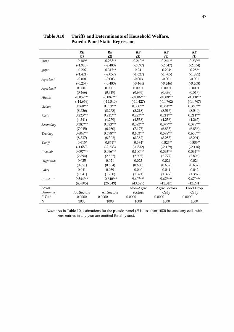
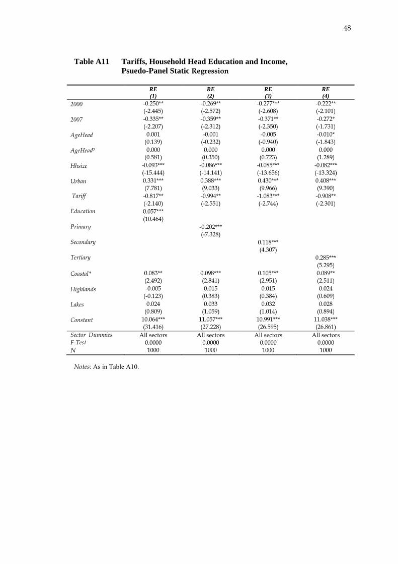
Comparable estimates for the pseudo-panel are in Table 12 (and in Tables

A10 and A11 excluding interaction terms). Although the size of the estimated

coefficients often differs, the sign and significance is generally the same with two

major differences. First, the coefficient on tariff is negative and significant (although

there are sector dummies): for representative households there is a negative

association between tariffs and incomes, probably reflecting the predominance of

agricultural households (note that the coefficients on Highlands and Lakes are now

28

insignificant but that for Coastal, the most urban region, is positive and significant).

Second, the coefficients on the year dummies are now negative and significant:

ceteris paribus, incomes of representative households have been declining. Other

results are supported: income decreases with household size, is higher in urban

locations, and increases with years of education (and the coefficient on

secondary*tariff is negative and significant). Households with no more than primary

education, mostly in agriculture, have lower incomes whereas households with

tertiary education have higher incomes; the coefficient on secondary education is

insignificant. The latter result seems to be because of the inclusion of the interaction

with tariffs, as all education variables are significant with the expected sign in Table

A10. These differences should be kept in mind for the dynamic estimates that require

the use of the pseudo-panel.

Dynamic Estimation

To allow for dynamics in the income equation, we re-estimate including the lagged

dependent variable and controlling for sector specific effects. As we are using the

pseudo-panel for the three survey rounds (1991/92, 2000/01 and 2007) the lagged

dependent variable is the income of the representative household cohort in the

preceding survey (so we have two waves for estimation). The results in Table 13

show that the lagged income term is generally significant, albeit weakly so, and

positive, suggesting a mild tendency for increasing income inequality. Table 14

reports the comparable results including education*tariff interaction terms (and the

coefficients on other variables are largely unaffected).

The estimates in Tables 13 and 14 confirm the results of the static model for the

pseudo-panel in Table 12; most estimated coefficients have almost the same values

with the exception of tariff (which has a much larger negative estimate). The

coefficient on tariff is negative and significant; given the significant positive

coefficients on urban and Coastal (the most urban region; the coefficient on Lakes is

weakly significant but Highlands remains insignificant), this is likely to reflect the

relatively high tariffs on agricultural products (especially cash crops). The coefficient

on the 2007 year dummy is negative and significant which is consistent with a decline

in cash crop incomes, ceteris paribus. There is clear support for the finding that

29

income increases with years of education in Table 13; the marginal impact of having

no more than primary education is actually negative (consistent with these being

mostly agriculture households).

Table 14 Marginal Impact Tariffs and Head Years of Education,

Dynamic Psuedo-Panel Regression RE

(1) RE (2)

RE (3)

RE (4)

2007

-0.225*** (-2.649)

-0.227*** (-2.585)

-0.257*** (-2.901)

-0.204** (-2.290)

Lag Welfare

0.054* (1.858)

0.066** (2.207)

0.063** (2.044)

0.056* (1.846)

AgeHead

0.005 (0.624)

0.007 (0.864)

0.012 (1.395)

-0.000 (-0.044)

AgeHead2

-0.0001 (-0.199)

-0.0001 (-0.791)

-0.0001 (-1.490)

-0.0001 (-0.270)

Hhsize

-0.097*** (-12.847)

-0.092*** (-11.913)

-0.090*** (-11.397)

-0.084*** (-10.855)

Urban

0.222*** (4.007)

0.294*** (5.248)

0.317*** (5.508)

0.277*** (4.767)

Tariff

-1.916*** (-3.073)

-2.005*** (-3.117)

-2.003*** (-3.064)

-2.049*** (-3.134)

Education

0.070*** (6.371)

Educ*Tariff

-0.093* (-1.655)

Primary

-0.275*** (-4.593)

Primary*Tariff

0.569* (1.627)

Secondary

0.011 (0.234)

Secondary*Tariff

-0.762*** (-2.801)

Tertiary

0.349*** (2.911)

Tertiary*Tariff

-0.210 (-0.306)

Coastal*

0.096*** (2.792)

0.110*** (3.096)

0.105*** (2.838)

0.096*** (2.606)

Highlands

-0.001 (-0.013)

0.016 (0.362)

0.008 (0.176)

0.026 (0.575)

Lakes

0.050 (1.641)

0.061* (1.952)

0.062* (1.934)

0.056* (1.749)

Constant

9.393*** (19.608)

9.726*** (19.544)

9.587*** (19.073)

9.919*** (19.916)

Sector Dummies All sectors All sectors All sectors All sectors F-Test 0.0000 0.0000 0.0000 0.0000 N 641 641 641 641

Notes: As in Table 13.

30

The one difference arises for the interaction terms in Table 14 as now the

coefficient on primary*tariff is positive and significant, while that on

secondary*tariff remains negative and significant. This suggests that, controlling for

lagged income, the interaction between tariffs and education differs between

agriculture and manufacturing. Agriculture households mostly have no more than

primary education; given that they have lower incomes, less educated producers of

products facing higher tariffs seem to have higher incomes than those producing

goods with lower tariffs (this may an effect of fishing, which is a larger share of

employment in the second two surveys, see Table A1a). The reverse association with

tariffs seems to apply to those with secondary education: ceteris paribus higher tariffs

are associated with lower incomes.

5 Conclusions and Discussion

The principal contribution of this paper is to identify the association between

household characteristics – in particular size and location, and for the household head

age, sector of employment and education - and household income using data from the

Tanzania Household Budget Survey for the years 1991/92, 2000/01 and 2007. A

specific aim was to identify the effect of trade policy so the analysis identified

households employed in traded sectors to permit addressing the effect of the cross-

sector pattern of tariff protection. About half the household heads surveyed, some

14,500 (about 2100, 8750 and 3640 in the respective years), were employed in traded

sectors. As the survey data are not a panel, the repeated cross-section for the three

rounds of Tanzania Household Budget Survey is exploited to construct a pseudo-

panel comprising 360 household cohorts (or representative households) for each

survey, defined according to the gender and age of the head and the location of the

household. Thus, while the static analysis of the determinants of household income is

based on the full sample of households, we are also able to conduct a dynamic

analysis using the pseudo-panel to provide a measure of lagged income (for the

representative household). The data are quite limited for the purposes of identifying

the effects of trade and trade policy on tariffs, as discussed below, so we begin by

reviewing the effects of other characteristics.

31

Descriptive analysis of the survey data in Section 3 suggests modest

increases in household income: on average, and for households whose primary source

of income is sales of food crops (the main source of income for about 40% of adults

in the sample), real income increased by 15% between 1991 and 2007. The largest

increases in income were for households earning income from sales of livestock and

livestock products (78% increase, but main source for less than 5% of adults),

business income (55% increase and this source doubled as a share from ten to 20 per

cent of adults) and informal employment (24%, but less than 5% of adults). The

largest sector in which household incomes fell, by four per cent overall (but 10%

between 2000 and 2007) was cash crop production, the main source of income for

over 20% of adults in 1991 but declining to 12% in 2007. This suggests that there are

important differences within agriculture, where most households are economically

active, and the econometric analysis (Section 4) accounts for sector of employment.

A number of household characteristics are consistent determinants of

income (measured as per adult equivalent real household expenditure), with similar

effects for estimates using all households and the pseudo-panel. Larger households

have lower income (income falls by about 7% for each additional family member);

living in urban areas is associated with higher income (around one quarter higher than

rural households); and location in the Coastal zone, which includes Dar es Salaam

(the business capital) but is also a major area for agriculture, increases household

income by about 15% compared to the poorest region (Central). Years of education of

the household head is associated with higher income: each additional year of

education adds about 4.5%, such that secondary education adds around 50% and

tertiary education over 75% to income compared with no education.

As tariffs are only levied on traded goods the sector-tariff analysis refers

to households whose head is employed in agriculture or manufacturing, although

households employed in non-traded sectors are treated as facing a zero tariff (so some

inferences can be drawn). Thus, we consider the effect of the cross-sector pattern of

protection (tariffs and changes in tariffs) on cross-sector variation in household

incomes. There are a number of limitations in the data for this purpose. First, and of

greatest importance, the sector of employment declared by the head may not capture

the sectors of activity of the household. Indeed, the distribution of head’s

32

employment across sectors does not tally well with reported sources of income or

sectors of activity of adults for the households. This is especially evident for cash

crops in 2000/01: fewer than three per cent of heads report this as their sector of

employment, but it is declared as the main source of income for 17% of adults. The

source of this problem is that households, as a group of adults, may be engaged in

many activities; an agriculture household may produce a combination of food, cash

crop and livestock products and some members may be engaged in off-farm business

or wage employment.

Second, and related, the tariff on a final product may not actually be

relevant to a household engaged in that sector, especially for agriculture. This is

particularly relevant for cash crops, as farmers typically produce for export in the

unprocessed form whereas associated imports, and hence tariffs, have undergone

some processing. A tariff on the unprocessed form may be redundant if that is not

actually imported (e.g. unroasted coffee beans), whereas a tariff on the processed

form (e.g. instant coffee) affects a manufacturing sector (e.g. Tanzanian producers of

instant coffee) and not the farmers. Although food crop sales compete with imports in

principle, in practice there may be some market segmentation (by quality, variety and

even location – with imports mainly in Dar-es-Salaam and local produce in rural

markets) and some food is produced for household own-consumption; any effect of

tariffs on food producers is at least dampened.

Third, trade and tariffs can affect households in many ways, the important

factors being production for export and the extent of competition from imports (and

tariffs are only one of the factors affecting domestic prices of import-competing

products). In particular, the main factors affecting demand and price for cash crop

exports are independent of Tanzanian tariffs, but it is export performance that drives

incomes. Furthermore, factors other than tariffs are likely to be the more important

determinants of sector performance and incomes; e.g. weather shocks or changes in

world (import) prices are important determinants of food crop incomes. The

relationship between tariffs and incomes will vary between sectors given the many

(unobserved) determinants of sector performance. As these product-specific factors

are unobserved the econometric analysis explicitly allows for sector differences

33

(through the use of sector dummies and interaction terms). Consequently, the results

for tariffs must be interpreted with great caution.

The estimated relationship between tariffs and incomes is found to be

sensitive to the treatment of sector effects and to the sample used (i.e. all households

as against the pseudo-panel of representative households). Overall there appears to be

a positive association between sector tariffs and household income, i.e. incomes

appear to be higher in sectors with higher tariffs. As agriculture is the main source of

income for more than half of households, and average incomes of agriculture

households are lower than for manufacturing households, it is especially important to

capture any agriculture effect. When this is done (using a dummy AGR = 1 if the head

of household is in agriculture and zero otherwise) the result suggests a negative effect

of tariffs in agriculture (with a much higher value of the positive coefficient for

manufactures compared to the negative coefficient for agriculture). However, within

agriculture at least, the relationship changes over time; for the reasons mentioned

above, this cannot be attributed to an effect of tariffs, especially as a wide range of

distortions affected agriculture (Morrissey and Leyaro, 2007). Tariffs have been

higher for cash crops than food crops; so too were average incomes in 1991 and 2001,

a positive correlation between tariffs and incomes, but by 2007 food crop incomes

exceeded those from cash crops (the correlation becomes negative). This is consistent

with a long-run tendency for food prices to increase faster than cash crop crises,

encouraging substitution into food crops (McKay et al, 1999).

In general, household income is increasing in both tariffs and education, and

the effect of tariffs diminishes, or becomes negative, as the level of education

increases, although the interaction term is only significant, and negative, for

secondary education. The marginal impact of tariffs on welfare is decreasing in level

of education as those with secondary education seem not to benefit from higher tariffs

(having secondary education does increase income). Household heads with secondary

and especially tertiary education are more likely to be employed in manufacturing so

the negative association between tariffs and secondary education is driven by effects

within manufacturing. Observing that tariffs offer less protection to the incomes of

more educated workers compared to less educated (less skilled) workers is consistent

34

with better educated workers being more productive and therefore in firms, or sectors,

better able to compete with imports.

Although tariffs may be positively associated with income across sectors

(even if this is due to the effect of particular sectors) this need not hold over time.

Within agriculture, there is some tendency for incomes to have risen faster in sectors

with lower tariffs (food crops) or where tariffs were reduced more (livestock

products), such that the correlation between tariffs and incomes was reversed.15 The

static estimates using all households did not capture this change in the correlation

over time but the pseudo-panel estimates appear to do so. For the pseudo-panel

estimates many factors have the same effects (e.g. household size and location) and

the effects for education are similar, but there are important exceptions, notably tariff

and the 2007 year dummy which have a negative association with incomes (but were

positive for the full household sample). The implication is that controlling for sector

effects, education and other household characteristics, and some unobserved tendency

for incomes to decline in 2007 given the income of the representative household in

the previous survey years, incomes were higher in those sectors with lower tariffs.

There is clearer support for the finding that income increases with years of

education in the pseudo-panel: the marginal impact of having no more than primary

education (mostly agriculture households) is positive, while that for secondary

education remains negative. The latter suggests that, within manufacturing, ceteris

paribus higher tariffs are associated with lower incomes. Given the same finding for

tariffs overall in the pseudo-panel, as noted above, the same seems to be true within

agriculture (and can be attributed to cash crops, which had high tariffs but declining

income).

For the reasons detailed earlier it would be incorrect to infer a causal

effect of tariffs on household incomes. Nevertheless, the analysis is informative about

the relationship between the cross-sector pattern of tariff protection (and changes in

tariffs) and household incomes. Within agriculture, incomes increased in the sector

with the lowest tariffs (food crops) but declined in the sector with the highest tariffs

(cash crops) so that the cross-sector correlation between tariffs and incomes switched

15 The decomposition of manufacturing sectors in the data is insufficient to explore similar effects within manufacturing as many of the specific sectors are relatively small in some years.

35

from positive to negative. A similar point may hold within manufacturing, i.e.

incomes may have been higher but fell faster or grew slower in sectors with relatively

high tariffs. As Tanzania implemented substantial tariff reductions in the past two

decades the distinction between correlations across sectors and over time is

important. However, it is likely that sector performance was determined, in large part

if not wholly, by factors other than tariffs.

There is quite consistent evidence that tariffs protect the incomes of less

educated (less skilled) workers more than they protect the incomes of more educated

workers. This is consistent with observing that import competition (and hence trade

liberalisation) presents a greater challenge to the incomes of relatively less educated

(less productive) workers. It may be true that at a global level trade liberalisation

benefits unskilled workers and developing countries, because workers in poorer

countries are less skilled than workers in richer countries, but within any country

more skilled or educated workers are more likely to benefit. The Stolper-Samuelson

theorem suggests that trade liberalisation should help the less skilled (who are likely

to be the less educated) and therefore the poor (although not the poorest) in

developing countries. There is little empirical evidence to support this, and most

evidence suggests that it is only the more skilled workers that benefit from trade

liberalisation. However, existing evidence is mostly limited to middle-income

developing countries, so we contribute by considering a low-income country. Thus,

the Stolper-Samuelson theorem may hold globally by favouring countries whose

labour is unskilled relative to the global average. However, within any developing

country it may be the less skilled that benefit least (or suffer most) from

liberalisation; in any country it is the more productive workers (who are more

educated and skilled) that are best able to benefit from international trade

opportunities. This is supported by our results for Tanzania: tariffs have tended to

protect the incomes of workers, more so for less educated workers so they may lose

most from liberalisation. Workers with secondary education seemed to benefit least

from tariff protection, so they may benefit more from liberalisation.

36

References

Ackah, C., O. Morrissey and S. Appleton (2007), ‘Who Gains from Trade Protection in Ghana: A Household-level Analysis’, School of Economics, University of Nottingham, CREDIT Research Paper 07/02.

Barraud, A. A. and G. Calfat (2008), ‘Poverty Effect from Trade Liberalisation in Argentina’, Journal of Development Studies, 44 (3), 365 - 383.

Bhagwati, J. and T.N. Srinivasan (2002), ‘Trade and Poverty in the Poor Countries’, AEA Papers and Proceedings, 92(2): 180-183.

Collado, M.D. (1998), ‘Estimating Binary Choice Models from Cohort Data’, Investigaciones Economicas, XXII (2), 259-276.

Davis, D. and P. Mishra (2007), ‘Stolper-Samuelson is Dead and Other Crimes of Both Theory and Data’, in Ann Harrison (ed), Globalization and Poverty, Chicago: University of Chicago Press for NBER

Deaton, A. (1985), ‘Panel Data from Time-Series of Cross-Sections’, Journal of Econometrics, 30(1-2), 109-126

Deaton, A. (1989), ‘Household Survey Data and Pricing Policies in Developing Countries’, World Bank Economic Review, 3(2), 183-210

Deaton, A. and F. Grimard (1992), ‘Demand Analysis for Tax Reform in Pakistan’, LMS Working Paper 85, World Bank, Washington DC.

Easterly, W. (2007) ‘Globalization, Prosperity, and Poverty, in Ann Harrison (ed), Globalization and Poverty, Chicago: University of Chicago Press for NBER

Edmonds, E. and N. Pavcnik (2002), ‘Does Globalization Increase Child Labor? Evidence from Vietnam’, Cambridge, MA: NBER Working Paper No. 8760

Fuhrer, J.C. (2000), ‘Habit Formation in Consumption and its Implications for Monetary Policy Models’, American Economic Review, 90 (1), 367-390.

Friedman, I. and J.A. Levinsohn (2002), ‘The Distributional Impact of Indonesia’s Financial Crisis on Household Welfare: A Rapid Response Methodology’, World Bank Economic Review, 16(3), 397-423.

Girma, S. (2000), ‘A Quasi-Differencing Approach to Dynamic Modelling from a Time Series of Independent Cross-Sections’, Journal of Econometrics, 98 (2), 365-383.

Goldberg, P. K. and N. Pavcnik (2007), ‘Distributional Effects of Globalization in Developing Countries,’ Journal of Economic Literature, 45(1): 39–82.

Harrison, A. (2006), ‘Globalisation and Poverty’, NBER Working Paper no. 12347, Cambridge, MA

Hertel, T. W. and R. J. Jeffrey (2004), ‘Poverty Impacts of Trade Reform’, Policy Research Working Paper no. 3444, World Bank, Washington DC

Kirkpatrick, C and S.S. Scrieciu (2007)’ ‘Caveat Emptor: The Computable General Equilibrium Approach to Assessing the Poverty Impact of Trade Liberalisation’, BWPI Working Paper no. 15, University of Manchester, Brooks World Poverty Institute

Kraay, A and D. Dollar (2004), ‘Trade, growth and poverty’, Economic Journal, 114(493), 22–49

Krueger, A. (1983), Trade and Employment in Developing Countries, Volume 3: Synthesis and Conclusions, Chicago: University of Chicago Press.

37

Leyaro, V., O. Morrissey and T. Owens (2010), ‘Food Price Changes and Consumer Welfare in Tanzania 1990-2007’, School of Economics, University of Nottingham: CREDIT Research Paper 10/01

McCulloch, N., A. Winters and X. Cirera (2002), Trade Liberalisation and Poverty: A Handbook, DfID and CEPR, London

Prasad, E. S., K. Rogoff, S-Jin Wei, and M. A. Kose (2007), ‘Effects of Financial Globalization on Developing Countries: Some Empirical Evidence, in Ann Harrison (ed), Globalization and Poverty, Chicago: University of Chicago Press for NBER

McKay, A., O. Morrissey and C. Vaillant (1999), ‘Aggregate Agricultural Supply Response in Tanzania’, Journal of International Trade and Economic Development 8(1), 107-123.

McKenzie, D. (2004), ‘Asymptotic theory for heterogeneous dynamic pseudo panels’, Journal of Econometrics, 120(2), 235-262.

Mofitt, R. (1993), ‘Identification and Estimation of Dynamic Models with a Time Series of Repeated Cross-Sections’, Journal of Econometrics, 59 (1-2), 99-123.

Morrissey, O. and V. Leyaro (2007), ‘Distortions to Agricultural Incentives in Tanzania’, Agricultural Distortions Research Project Working Paper 52, Washington DC, The World Bank, pp. 307-328. Shorter version in K. Anderson and W. Masters (eds.) (2009), Distortions to Agricultural Incentives in Africa, Washington DC: World Bank, chapter 11, pp. 307-328.

National Bureau of Statistics (2002), Tanzania Household Budget Surveys for 1991/ 92 and 2000/01, Dar-es-Salaam: National Bureau of Statistics, United Republic of Tanzania.

National Bureau of Statistics (2008), Tanzania Household Budget Surveys for 1991/ 92, 2000/01 and 2007, Dar-es-Salaam: National Bureau of Statistics, United Republic of Tanzania.

Nicita, A. (2004), ‘Who Benefited from Trade Liberalization in Mexico: Measuring the Effects on Household Welfare’, World Bank Policy Research Working Paper No. 3265, Washington D.C., World Bank

Porto, G. G. (2006), ‘Using Survey Data to Assess the Distributional Effects of Trade Policy’, Journal of International Economics, 70(1), 140-160.

Ravallion, M. (2004), ‘Looking Beyond Averages in the Trade and Poverty Debate’, Policy Research Working Paper 3461, World Bank Washington D.C.

Reimer, J.J. (2002), ‘Estimating the Poverty Impacts of Trade Liberalization’, Policy Research Working Paper no. 2790, World Bank, Washington DC

Sala-i-Martin, X. (2002), ‘The Disturbing 'Rise' of Global Income Inequality’, Cambridge, MA: National Bureau of Economic Research, NBER Working Paper no. 8904

Seshan, G. (2005), ‘The Impact o Trade Liberalisation on Household Welfare in Vietnam’, Policy Research Working Paper No. 3541, World Bank, Washington, D.C.

Topalova, P. (2004), Trade Liberalization, Poverty and Inequality: Evidence from Indian Districts, Chicago: University of Chicago Press for NBER.

Treichel, V. (2005), ‘Tanzania’s Growth Process and Success in Reducing Poverty’, IMF Working Paper No. 05/35, IMF African Department.

Van de Walle, D. and D. Cratty (2003), ‘Is the Emerging Non-Farm Market Economy the Route Out of Poverty in Vietnam?’, Policy Research Working Paper no. 2950, Development Research Group, World Bank, Washington, D.C.

38

Verbeek, M. and F. Vella (2005), ‘Estimating Dynamic Models from Repeated Cross-Sections’, Journal of Econometrics, 127 (1), 83-102.

Winters, L. A. (2002), ‘Trade, Trade Policy and Poverty: What are the Links’, World Economy, 25(9): 1339-1367.

Winters, A. L., N. McCulloch and A. McKay (2004), ‘Trade Liberalization and Poverty: the Evidence So Far’, Journal of Economic Literature, XLII (March), 72-115.

39

APPENDIX TABLES

Table A1 Average Tariff Rates by Commodity Groups

No.

Sectors

Scheduled Applied

1991

2000

2007

1991

2000

2007 1 Food Crops 0.30 0.14 0.076 0.1032 0.1588 0.0887 2 Livestock 0.40 0.25 0.125 0.2258 0.1964 0.1301 3 Cash crops 0.50 0.23 0.115 0.2499 0.17644 0.2230 4 Fishing 0.40 0.25 0.125 0.1588 0.0968 0.2415 5 Manufactured food 0.50 0.23 0.115 0.2281 0.2326 0.2321 6 Dairy 0.40 0.24 0.122 0.2771 0.2179 0.3026 7 Textile 0.50 0.23 0.115 0.1756 0.1031 0.1662 8 Timber and Wood 0.50 0.23 0.115 0.2267 0.1655 0.1327 9 Paper 0.50 0.23 0.115 0.1888 0.0818 0.0795 10 Chemicals 0.50 0.23 0.115 0.0170 0.0151 0.0300 11 Other Manufacture 0.50 0.23 0.115 0.2833 0.2224 0.2398 12 Sports goods 0.50 0.23 0.115 0.2371 0.2174 0.2331 13 Building materials 0.50 0.23 0.115 0.1513 0.1546 0.1258

Notes: Tariffs are ad valorem as reported in Tariff book (scheduled) or calculated as tariff revenue as a

share of import value (applied or implicit). Non-traded sectors (e.g. wholesale and retail, hotels and restaurants, electricity) are omitted on the basis that the tariff is undefined.

Source: Tanzania Revenue Authority, Customs Department Table A1a Sector Shares for Household Employment - 1991/92, 2000/01 and

2007 Surveys

No.

Sectors

1991/92

2000/01

2007

1 Food crops 21.63 20.76 26.39 2 Livestock and livestock products 2.39 1.87 2.42 3 Cash crops 12.34 2.60 9.96 4 Fishing 1.81 4.52 3.49 5 Food manufactures 4.25 8.87 0.35 6 Dairy 0.31 0.04 0.67 7 Textile 0.82 1.99 4.01 8 Timber and wood 1.29 2.92 4.06 9 Paper 0.66 0.10 1.41 10 Chemicals 0.59 1.11 0.41 11 Other manufactures 1.34 0.62 0.06 12 Sports goods 0.75 0.27 0.20 13 Building materials 1.27 2.35 2.23 14 All Others (non-traded) 50.56 51.96 44.34 Total (Total sample size) 100 (4,262) 100 (18,243) 100 (6,534)

Notes: Households allocated to sectors as classified in Table A1

40

Table A2 Economic Activity and Level of Education, 2000/01

Activity Education of Household Head

Primary Secondary Tertiary All Farming, livestock or fishing 0.97 0.02 0.00 1.0

Employee – government 0.38 0.51 0.10 1.0

Employee – parastatals 0.52 0.33 0.15 1.0

Employee – other 0.68 0.26 0.06 1.0

Self-employed with employees 0.87 0.12 0.01 1.0

Self-employed no employees 0.83 0.15 0.02 1.0

Others 0.86 0.11 0.03 1.0 Notes: ‘Primary’ is no education up to completed primary, and includes adult education as less than

primary. Secondary includes post-secondary. Source: Authors’ calculation from Tanzania Household Budget Survey for the years 1991/92,

2000/01 and 2007 Table A3 Economic Activity and Level of Education, 2007

Activity

Education of Household Head

Primary Secondary Tertiary All Farming, livestock or fishing 0.96 0.04 0.00 1.0Employee – government 0.35 0.43 0.22 1.0Employee – parastatals na na na naEmployee – other 0.60 0.24 0.15 1.0Self-employed with employees 0.78 0.15 0.07 1.0Self-employed no employees 0.90 0.09 0.01 1.0Others 0.80 0.16 0.03 1.0

Notes and Source: As for Table A2

41

Table A4 Source of Income and Level of Education, 2000/01

Source of income Education of Household Head

Primary Secondary Tertiary All Sales of food crops 0.97 0.03 0.00 1.0

Sales of livestock & products 0.98 0.02 0.00 1.0

Sales of cash crops 0.97 0.03 0.00 1.0

Business income 0.88 0.11 0.01 1.0

Wages or salaries in cash 0.55 0.37 0.08 1.0

Other casual cash earning 0.84 0.15 0.01 1.0

Cash remittances 0.92 0.03 0.05 1.0

Fishing 0.98 0.02 0.00 1.0

Other 0.92 0.05 0.02 1.0 Notes and Source: As for Table A2 TableA5 Source of Income and Level of Education, 2007

Source of income

Education of Household Head

Primary Secondary Tertiary All

Sales of food crops 0.97 0.03 0.00 1.0

Sales of livestock & products 0.93 0.05 0.01 1.0

Sales of cash crops 0.97 0.03 0.01 1.0

Business income 0.95 0.05 0.01 1.0

Wages or salaries in cash 0.64 0.24 0.11 1.0

Other casual cash earning 0.94 0.04 0.02 1.0

Cash remittances 0.94 0.04 0.02 1.0

Fishing 0.95 0.05 0.00 1.0

Other 0.91 0.09 0.00 1.0 Notes and Source: As for Table A2

42

Table A6 Saturated Model, All Sectors Interacted with Tariffs and Education POLS

(1) RE (2)

POLS (3)

RE (4)

2000

0.032*** (2.681)

0.063*** (4.597)

2000

0.034*** (2.865)

0.062*** (4.544)

2007

0.154*** (9.446)

0.143*** (7.565)

2007

0.146*** (9.038)

0.134*** (7.126)

AgeHead

-0.018*** (-7.884)

-0.018*** (-6.107)

AgeHead

-0.017*** (-7.300)

-0.017*** (-5.657)

AgeHead2

0.0001***

(6.811) 0.0001*** (5.588)

AgeHead2

0.0001*** (6.844)

0.0001*** (5.595)

Hhsize

-0.078*** (-47.505)

-0.077*** (-65.798)

Hhsize

-0.078*** (-47.494)

-0.077*** (-65.936)

Urban

0.240*** (29.675)

0.233*** (28.742)

Urban

0.229*** (28.173)

0.221*** (27.249)

Basic*

0.200*** (19.267)

0.196*** (18.965)

Basic*

0.036** (2.287)

0.040** (2.561)

Secondary

0.520*** (36.199)

0.503*** (35.610)

Secondary

0.167*** (5.954)

0.165*** (6.071)

Post Secondary

0.624*** (33.622)

0.599*** (31.055)

Post Secondary

0.194*** (5.624)

0.187*** (5.492)

Tertiary

0.802*** (40.875)

0.776*** (41.712)

Tertiary

0.244*** (5.740)

0.241*** (5.922)

Tariff

0.712** (2.415)

0.760*** (2.705)

Tariff

0.285*** (4.329)

0.244*** (3.724)

SCTR1

0.118* (1.675)

0.134* (1.919)

SCTR1

-0.254*** (-7.362)

-0.249*** (-7.400)

SCTR2

-0.088 (-1.226)

-0.054 (-0.757)

SCTR2

-0.455*** (-14.597)

-0.431*** (-14.153)

SCTR3

0.163* (1.812)

0.168* (1.892)

SCTR3

-0.302*** (-6.513)

-0.306*** (-6.783)

SCTR4

-0.135* (-1.781)

-0.070 (-0.933)

SCTR4

-0.389*** (-9.960)

-0.372*** (-10.043)

SCTR5

-0.133 (-1.527)

-0.084 (-0.985)

SCTR5

-0.385*** (-9.357)

-0.351*** (-8.849)

SCTR6

0.117 (1.363)

0.102 (1.197)

SCTR6

-0.291*** (-7.870)

-0.278*** (-7.655)

SCTR7

0.398*** (3.334)

0.413*** (2.877)

SCTR7

-0.305** (-2.431)

-0.324** (-2.270)

SCTR8

0.192** (2.200)

0.202** (2.267)

SCTR8

-0.172*** (-2.747)

-0.170*** (-2.993)

SCTR9

-0.076 (-0.901)

-0.027 (-0.318)

SCTR9

-0.476*** (-10.822)

-0.451*** (-9.918)

SCTR10

0.201* (1.689)

0.234** (2.106)

SCTR10

-0.436*** (-5.015)

-0.400*** (-4.601)

SCTR11

0.207 (1.339)

0.225* (1.727)

SCTR11

-0.253*** (-2.900)

-0.240*** (-3.036)

SCTR12

0.427*** (2.693)

0.411*** (2.896)

SCTR12

-0.304** (-2.477)

-0.278*** (-2.659)

SCTR13

0.211 (1.315)

0.219 (1.409)

SCTR13

-0.163 (-1.157)

-0.155 (-1.285)

Tariff*SCTR1

0.000

.

0.000

.

Educn* SCTR1

0.034*** (14.507)

0.032*** (14.382)

43

Tariff*SCTR2

-0.660** (-2.189)

-0.720** (-2.494)

Educn* SCTR2

0.025*** (8.959)

0.025*** (9.034)

Tariff*SCTR3

-0.830** (-2.384)

-0.871** (-2.574)

Educn* SCTR3

0.034*** (5.752)

0.035*** (5.858)

Tariff*SCTR4

-0.062 (-0.202)

-0.243 (-0.831)

Educn* SCTR4

0.033*** (7.937)

0.034*** (8.426)

Tariff*SCTR5

-0.044 (-0.120)

-0.157 (-0.462)

Educn* SCTR5

0.031*** (6.522)

0.029*** (6.302)

Tariff*SCTR6

-0.814** (-2.406)

-0.714** (-2.171)

Educn* SCTR6

0.022*** (5.548)

0.023*** (6.056)

Tariff*SCTR7

-1.502*** (-3.368)

-1.491*** (-2.720)

Educn* SCTR7

0.043*** (3.388)

0.047*** (3.501)

Tariff*SCTR8

-0.312 (-0.851)

-0.370 (-1.006)

Educn* SCTR8

0.035*** (5.369)

0.034*** (5.992)

Tariff*SCTR9

-0.287 (-0.821)

-0.409 (-1.171)

Educn* SCTR9

0.044*** (9.099)

0.044*** (8.415)

Tariff*SCTR10

-0.801 (-1.604)

-0.914** (-2.112)

Educn* SCTR10

0.062*** (5.473)

0.057*** (5.835)

Tariff*SCTR11

-1.027* (-1.704)

-1.033** (-2.121)

Educn* SCTR11

0.025*** (3.051)

0.026*** (3.469)

Tariff*SCTR12

-1.077** (-2.098)

-1.059** (-2.357)

Educn* SCTR12

0.049*** (3.593)

0.045*** (4.186)

Tariff*SCTR13

-0.910* (-1.952)

-0.987** (-2.149)

Educn* SCTR13

0.013 (0.722)

0.011 (0.810)

Coastal* 0.159*** (14.745)

0.141*** (6.285) Coastal*

0.159*** (14.826)

0.141*** (6.186)

Highlands 0.055*** (4.883)

0.062*** (2.741) Highlands

0.055*** (4.927)

0.063*** (2.727)

Lakes 0.049*** (4.084)

0.055** (2.362) Lakes

0.052*** (4.360)

0.056** (2.379)

Constant 9.725***

(109.785) 9.669*** (97.074) Constant

10.002*** (160.418)

9.966*** (129.170)

F-Test 0.000 0.000 F-Test 0.000 0.000 R2 0.354 R2 0.359 N 28031 28031 N 27976 27976

Notes: As for RE in Table 10

44

Table A7 Distinguishing Agriculture and Manufacturing Effects POLS

(1) RE (2)

2000

0.035*** (2.967)

0.065*** (4.824)

2007

0.153*** (9.389)

0.142*** (7.543)

AgeHead

-0.018*** (-7.894)

-0.018*** (-6.162)

AgeHead2

0.000*** (6.820)

0.000*** (5.642)

Hhsize

-0.078*** (-47.471)

-0.077*** (-65.811)

Urban

0.241*** (29.755)

0.233*** (28.813)

Basic*

0.200*** (19.255)

0.196*** (18.967)

Secondary

0.520*** (36.198)

0.503*** (35.627)

Post Secondary

0.625*** (33.630)

0.600*** (31.095)

Tertiary

0.803*** (40.867)

0.776*** (41.731)

Tariff

0.520*** (6.106)

0.432*** (5.183)

AGR

-0.132*** (-3.942)

-0.130*** (-3.890)

Tariff*AGR

-0.470*** (-4.364)

-0.391*** (-3.698)

MANF

0.131** (2.008)

0.161** (2.021)

Tariff*MANF

-0.483*** (-3.877)

-0.359*** (-2.926)

Coastal*

0.160*** (14.799)

0.141*** (6.312)

Highlands

0.056*** (4.989)

0.062*** (2.776)

Lakes

0.049*** (4.123)

0.055** (2.367)

Constant

9.767*** (157.765)

9.746*** (127.043)

Sector Dummies All All F-Test 0.0000 0.0000 R2 0.353 N 28031 28031

Notes: As for RE in Table 10

45

Table A8 Tariffs and Head Years of Education, Cohort Panel Static Regression RE

(1) RE (2)

RE (3)

RE (4)

2000

0.043*** (3.346)

0.063*** (4.867)

0.071*** (5.430)

0.062*** (4.703)

2007

0.100*** (5.715)

0.141*** (7.994)

0.143*** (7.972)

0.132*** (7.254)

AgeHead

-0.015*** (-5.045)

-0.017*** (-5.850)

-0.015*** (-4.854)

-0.016*** (-5.349)

AgeHead2

0.000*** (5.322)

0.000*** (4.767)

0.000*** (3.692)

0.000*** (3.937)

Hhsize

-0.078*** (-66.607)

-0.076*** (-64.250)

-0.076*** (-62.413)

-0.076*** (-62.669)

Urban

0.217*** (26.951)

0.254*** (31.518)

0.275*** (33.431)

0.293*** (35.935)

Tariff

0.220*** (4.440)

0.193*** (3.836)

0.171*** (3.334)

0.102** (1.997)

AGR

-0.178*** (-8.629)

-0.192*** (-9.186)

-0.226*** (-10.582)

-0.220*** (-10.338)

Tariff*AGR

-0.192** (-2.068)

-0.178* (-1.886)

-0.151* (-1.664)

-0.168* (-1.751)

Education

0.045*** (55.303)

Primary

-0.405*** (-46.034)

Secondary 0.299*** (30.734)

Tertiary 0.510*** (30.984)

Coastal*

0.138*** (5.871)

0.149*** (6.491)

0.151*** (6.551)

0.145*** (5.988)

Highlands

0.059** (2.500)

0.077*** (3.355)

0.083*** (3.572)

0.086*** (3.521)

Lakes

0.054** (2.233)

0.065*** (2.729)

0.069*** (2.900)

0.070*** (2.795)

Constant

9.667*** (138.387)

10.357*** (147.243)

9.913*** (140.087)

9.997*** (138.729)

Sector Dummies

Non-Agric

Non-Agric

Non-Agric

Non-Agric

F-Test 0.0000 0.0000 0.0000 0.0000 N 27976 28031 28031 28031 Notes: As in Table 10 Comment: In the table households are in three groups: those with no more than primary education (includes adult education) can be thought of as unskilled; those with secondary and post-secondary education can be thought of as semi-skilled; and those with tertiary education can be thought of as skilled. A low level of education (primary) is negative and statistically significant, implying it is associated with low income. Higher education, secondary and above, is positive and significant, implying association with higher income. This is consistent with the observation that income increases with skill level.

46

Table A9 Marginal Impacts of Tariffs and Head Years of Education, Pooled Cross-section Static Regression POLS

(1) POLS

(2) POLS

(3) POLS

(4) 2000

0.021* (1.847)

0.025** (2.223)

0.018 (1.588)

0.019* (1.680)

2007

0.119*** (8.168)

0.142*** (9.643)

0.132*** (8.815)

0.129*** (8.681)

AgeHead

-0.016*** (-7.067)

-0.017*** (-7.144)

-0.012*** (-5.177)

-0.014*** (-5.984)

AgeHead2

0.000*** (6.992)

0.000*** (5.451)

0.000*** (3.451)

0.000*** (3.855)

Hhsize

-0.079*** (-47.832)

-0.076*** (-47.429)

-0.075*** (-46.961)

-0.075*** (-46.805)

Urban

0.226*** (28.090)

0.264*** (32.684)

0.284*** (34.688)

0.305*** (37.168)

Tariff

0.237*** (4.745)

0.228*** (4.486)

0.660*** (8.707)

0.142*** (2.772)

AGR

-0.188*** (-9.102)

-0.208*** (-10.029)

-0.252*** (-12.008)

-0.242*** (-11.481)

Tariff*AGR

-0.256*** (-2.715)

-0.230** (-2.430)

-0.150* (-1.678)

-0.215** (-2.252)

Education

0.049*** (50.285)

Education*Tariff

-0.032*** (-5.569)

Primary

-0.433*** (-42.156)

Primary*Tariff

0.088 (1.168)

Secondary

0.274*** (25.494)

Secondary*Tariff

-0.661*** (-8.478)

Tertiary

0.537*** (27.965)

Tertiary*Tariff

0.038 (0.241)

Coastal*

0.155*** (14.472)

0.172*** (15.840)

0.180*** (16.231)

0.171*** (15.290)

Highlands

0.051*** (4.576)

0.070*** (6.185)

0.075*** (6.526)

0.081*** (7.007)

Lakes

0.049*** (4.167)

0.059*** (4.895)

0.064*** (5.219)

0.065*** (5.261)

Constant

9.697*** (191.134)

10.408*** (199.470)

9.931*** (190.662)

10.004*** (191.102)

Sector Dummies Non-Agric Non-Agric Non-Agric Non-Agric F-Test 0.0000 0.0000 0.0000 0.0000 R2 0.359 0.337 0.310 0.308 N 27976 28031 28031 28031 Notes: As in Table 10

47

Table A10 Tariffs and Determinants of Household Welfare, Psuedo-Panel Static Regression

RE (1)

RE (2)

RE (3)

RE (4)

RE (1)

2000

-0.189* (-1.913)

-0.258** (-2.488)

-0.210** (-2.097)

-0.244** (-2.347)

-0.239** (-2.334)

2007

-0.207 (-1.421)

-0.317** (-2.057)

-0.241 (-1.627)

-0.294* (-1.905)

-0.286* (-1.881)

AgeHead

-0.001 (-0.237)

-0.003 (-0.480)

-0.003 (-0.464)

-0.001 (-0.246)

-0.001 (-0.268)

AgeHead2

0.0001 (0.466)

0.0001 (0.719)

0.0001 (0.676)

0.0001 (0.499)

0.0001 (0.517)

Hhsize

-0.087*** (-14.659)

-0.087*** (-14.540)

-0.086*** (-14.427)

-0.088*** (-14.762)

-0.088*** (-14.767)

Urban

0.360*** (8.536)

0.353*** (8.278)

0.350*** (8.218)

0.361*** (8.516)

0.360*** (8.540)

Basic

0.223*** (4.541)

0.211*** (4.279)

0.223*** (4.558)

0.211*** (4.256)

0.211*** (4.267)

Secondary

0.387*** (7.045)

0.383*** (6.980)

0.393*** (7.177)

0.377*** (6.833)

0.378*** (6.856)

Tertiary

0.604*** (8.337)

0.598*** (8.302)

0.603*** (8.382)

0.598*** (8.253)

0.600*** (8.291)

Tariff

-0.615* (-1.680)

-0.861** (-2.233)

-0.684* (-1.832)

-0.823** (-2.129)

-0.806** (-2.116)

Coastal*

0.097*** (2.894)

0.096*** (2.862)

0.100*** (2.997)

0.093*** (2.777)

0.094*** (2.806)

Highlands

0.025 (0.651)

0.021 (0.564)

0.023 (0.608)

0.024 (0.637)

0.024 (0.637)

Lakes

0.041 (1.341)

0.039 (1.280)

0.040 (1.321)

0.041 (1.327)

0.042 (1.387)

Constant

9.544*** (43.805)

10.640*** (26.349)

9.607*** (43.825)

9.676*** (41.343)

9.670*** (42.294)

Sector Dummies

No Sectors

All Sectors

Non-Agric Sectors

Agric Sectors Only

Food Crop Only

F-Test 0.0000 0.0000 0.0000 0.0000 0.0000 N 1000 1000 1000 1000 1000

Notes: As in Table 10, estimations for the pseudo-panel (N is less than 1080 because any cells with

zero entries in any year are omitted for all years).

48

Table A11 Tariffs, Household Head Education and Income, Psuedo-Panel Static Regression

RE (1)

RE (2)

RE (3)

RE (4)

2000

-0.250** (-2.445)

-0.269** (-2.572)

-0.277*** (-2.608)

-0.222** (-2.101)

2007

-0.335** (-2.207)

-0.359** (-2.312)

-0.371** (-2.350)

-0.272* (-1.731)

AgeHead

0.001 (0.139)

-0.001 (-0.232)

-0.005 (-0.940)

-0.010* (-1.843)

AgeHead2

0.000

(0.581) 0.000

(0.350) 0.000

(0.723) 0.000

(1.289) Hhsize

-0.093*** (-15.444)

-0.086*** (-14.141)

-0.085*** (-13.656)

-0.082*** (-13.324)

Urban

0.331*** (7.781)

0.388*** (9.033)

0.430*** (9.966)

0.408*** (9.390)

Tariff

-0.817** (-2.140)

-0.994** (-2.551)

-1.083*** (-2.744)

-0.908** (-2.301)

Education 0.057*** (10.464)

Primary -0.202*** (-7.328)

Secondary 0.118*** (4.307)

Tertiary 0.285*** (5.295)

Coastal*

0.083** (2.492)

0.098*** (2.841)

0.105*** (2.951)

0.089** (2.511)

Highlands

-0.005 (-0.123)

0.015 (0.383)

0.015 (0.384)

0.024 (0.609)

Lakes

0.024 (0.809)

0.033 (1.059)

0.032 (1.014)

0.028 (0.894)

Constant

10.064*** (31.416)

11.057*** (27.228)

10.991*** (26.595)

11.038*** (26.861)

Sector Dummies All sectors All sectors All sectors All sectors F-Test 0.0000 0.0000 0.0000 0.0000 N 1000 1000 1000 1000

Notes: As in Table A10.

49

Table A12: Cohort Definition, 5-year Age Bands

Cohort ID Region of Domicile Age in 1991/92 Age in 2000/01 Age in 20007 Sex Head

Mean Cell Size 1 Dodoma 18-22 27-31 34-38 Male 148 2 Dodoma 23-27 32-36 39-43 Male 172 3 Dodoma 28-32 37-41 44-48 Male 160 4 Dodoma 33-37 42-46 49-53 Male 50 5 Dodoma 38-42 47-51 54-58 Male 126 6 Dodoma 43-47 52-56 59-63 Male 96 7 Dodoma 48-52 57-61 64-68 Male 74 8 Dodoma 53-57 62-66 69-73 Male 57 9 Dodoma 58-62 67-71 74-78 Male 40 10 Dodoma 18-22 27-31 34-38 Female 54 11 Dodoma 23-27 32-36 39-43 Female 59 12 Dodoma 28-32 37-41 44-48 Female 55 13 Dodoma 33-37 42-46 49-53 Female 50 14 Dodoma 38-42 47-51 54-58 Female 42 15 Dodoma 43-47 52-56 59-63 Female 28 16 Dodoma 48-52 57-61 64-68 Female 30 17 Dodoma 53-57 62-66 69-73 Female 19 18 Dodoma 58-62 67-71 74-78 Female 14 19 Arusha 18-22 27-31 34-38 Male 226 20 Arusha 23-27 32-36 39-43 Male 239 21 Arusha 28-32 37-41 44-48 Male 206 22 Arusha 33-37 42-46 49-53 Male 182 23 Arusha 38-42 47-51 54-58 Male 139 24 Arusha 43-47 52-56 59-63 Male 77 25 Arusha 48-52 57-61 64-68 Male 46 26 Arusha 53-57 62-66 69-73 Male 39 27 Arusha 58-62 67-71 74-78 Male 41 28 Arusha 18-22 27-31 34-38 Female 61 29 Arusha 23-27 32-36 39-43 Female 59 30 Arusha 28-32 37-41 44-48 Female 60 31 Arusha 33-37 42-46 49-53 Female 32 32 Arusha 38-42 47-51 54-58 Female 35 33 Arusha 43-47 52-56 59-63 Female 22 34 Arusha 48-52 57-61 64-68 Female 13 35 Arusha 53-57 62-66 69-73 Female 11 36 Arusha 58-62 67-71 74-78 Female 8 37 Kilimanjaro 18-22 27-31 34-38 Male 108 38 Kilimanjaro 23-27 32-36 39-43 Male 143 39 Kilimanjaro 28-32 37-41 44-48 Male 177 40 Kilimanjaro 33-37 42-46 49-53 Male 149 41 Kilimanjaro 38-42 47-51 54-58 Male 138 42 Kilimanjaro 43-47 52-56 59-63 Male 92 43 Kilimanjaro 48-52 57-61 64-68 Male 72 44 Kilimanjaro 53-57 62-66 69-73 Male 50 45 Kilimanjaro 58-62 67-71 74-78 Male 48 46 Kilimanjaro 18-22 27-31 34-38 Female 55 47 Kilimanjaro 23-27 32-36 39-43 Female 59 48 Kilimanjaro 28-32 37-41 44-48 Female 67 49 Kilimanjaro 33-37 42-46 49-53 Female 52 50 Kilimanjaro 38-42 47-51 54-58 Female 31 51 Kilimanjaro 43-47 52-56 59-63 Female 28 52 Kilimanjaro 48-52 57-61 64-68 Female 17 53 Kilimanjaro 53-57 62-66 69-73 Female 10 54 Kilimanjaro 58-62 67-71 74-78 Female 14 55 Tanga 18-22 27-31 34-38 Male 148 56 Tanga 23-27 32-36 39-43 Male 173 57 Tanga 28-32 37-41 44-48 Male 207 58 Tanga 33-37 42-46 49-53 Male 145 59 Tanga 38-42 47-51 54-58 Male 144 60 Tanga 43-47 52-56 59-63 Male 88 61 Tanga 48-52 57-61 64-68 Male 73 62 Tanga 53-57 62-66 69-73 Male 64

50

63 Tanga 58-62 67-71 74-78 Male 62 64 Tanga 18-22 27-31 34-38 Female 43 65 Tanga 23-27 32-36 39-43 Female 53 66 Tanga 28-32 37-41 44-48 Female 42 67 Tanga 33-37 42-46 49-53 Female 57 68 Tanga 38-42 47-51 54-58 Female 57 69 Tanga 43-47 52-56 59-63 Female 27 70 Tanga 48-52 57-61 64-68 Female 22 71 Tanga 53-57 62-66 69-73 Female 19 72 Tanga 58-62 67-71 74-78 Female 5 73 Morogoro 18-22 27-31 34-38 Male 178 74 Morogoro 23-27 32-36 39-43 Male 210 75 Morogoro 28-32 37-41 44-48 Male 183 76 Morogoro 33-37 42-46 49-53 Male 174 77 Morogoro 38-42 47-51 54-58 Male 129 78 Morogoro 43-47 52-56 59-63 Male 103 79 Morogoro 48-52 57-61 64-68 Male 71 80 Morogoro 53-57 62-66 69-73 Male 48 81 Morogoro 58-62 67-71 74-78 Male 42 82 Morogoro 18-22 27-31 34-38 Female 41 83 Morogoro 23-27 32-36 39-43 Female 34 84 Morogoro 28-32 37-41 44-48 Female 51 85 Morogoro 33-37 42-46 49-53 Female 34 86 Morogoro 38-42 47-51 54-58 Female 39 87 Morogoro 43-47 52-56 59-63 Female 24 88 Morogoro 48-52 57-61 64-68 Female 24 89 Morogoro 53-57 62-66 69-73 Female 21 90 Morogoro 58-62 67-71 74-78 Female 11 91 Pwani 18-22 27-31 34-38 Male 117 92 Pwani 23-27 32-36 39-43 Male 127 93 Pwani 28-32 37-41 44-48 Male 124 94 Pwani 33-37 42-46 49-53 Male 104 95 Pwani 38-42 47-51 54-58 Male 108 96 Pwani 43-47 52-56 59-63 Male 65 97 Pwani 48-52 57-61 64-68 Male 66 98 Pwani 53-57 62-66 69-73 Male 53 99 Pwani 58-62 67-71 74-78 Male 33 100 Pwani 18-22 27-31 34-38 Female 37 101 Pwani 23-27 32-36 39-43 Female 28 102 Pwani 28-32 37-41 44-48 Female 34 103 Pwani 33-37 42-46 49-53 Female 36 104 Pwani 38-42 47-51 54-58 Female 21 105 Pwani 43-47 52-56 59-63 Female 26 106 Pwani 48-52 57-61 64-68 Female 18 107 Pwani 53-57 62-66 69-73 Female 27 108 Pwani 58-62 67-71 74-78 Female 14 109 Dar es salaam 18-22 27-31 34-38 Male 581 110 Dar es salaam 23-27 32-36 39-43 Male 469 111 Dar es salaam 28-32 37-41 44-48 Male 471 112 Dar es salaam 33-37 42-46 49-53 Male 515 113 Dar es salaam 38-42 47-51 54-58 Male 484 114 Dar es salaam 43-47 52-56 59-63 Male 289 115 Dar es salaam 48-52 57-61 64-68 Male 169 116 Dar es salaam 53-57 62-66 69-73 Male 211 117 Dar es salaam 58-62 67-71 74-78 Male 62 118 Dar es salaam 18-22 27-31 34-38 Female 132 119 Dar es salaam 23-27 32-36 39-43 Female 104 120 Dar es salaam 28-32 37-41 44-48 Female 120 121 Dar es salaam 33-37 42-46 49-53 Female 99 122 Dar es salaam 38-42 47-51 54-58 Female 74 123 Dar es salaam 43-47 52-56 59-63 Female 40 124 Dar es salaam 48-52 57-61 64-68 Female 9 125 Dar es salaam 53-57 62-66 69-73 Female 14 126 Dar es salaam 58-62 67-71 74-78 Female 11 127 Lindi 18-22 27-31 34-38 Male 139 128 Lindi 23-27 32-36 39-43 Male 144 129 Lindi 28-32 37-41 44-48 Male 130 130 Lindi 33-37 42-46 49-53 Male 96

51

131 Lindi 38-42 47-51 54-58 Male 90 132 Lindi 43-47 52-56 59-63 Male 76 133 Lindi 48-52 57-61 64-68 Male 51 134 Lindi 53-57 62-66 69-73 Male 39 135 Lindi 58-62 67-71 74-78 Male 33 136 Lindi 18-22 27-31 34-38 Female 49 137 Lindi 23-27 32-36 39-43 Female 35 138 Lindi 28-32 37-41 44-48 Female 34 139 Lindi 33-37 42-46 49-53 Female 33 140 Lindi 38-42 47-51 54-58 Female 27 141 Lindi 43-47 52-56 59-63 Female 26 142 Lindi 48-52 57-61 64-68 Female 23 143 Lindi 53-57 62-66 69-73 Female 18 144 Lindi 58-62 67-71 74-78 Female 14 145 Mtwara 18-22 27-31 34-38 Male 141 146 Mtwara 23-27 32-36 39-43 Male 163 147 Mtwara 28-32 37-41 44-48 Male 186 148 Mtwara 33-37 42-46 49-53 Male 126 149 Mtwara 38-42 47-51 54-58 Male 125 150 Mtwara 43-47 52-56 59-63 Male 96 151 Mtwara 48-52 57-61 64-68 Male 77 152 Mtwara 53-57 62-66 69-73 Male 48 153 Mtwara 58-62 67-71 74-78 Male 41 154 Mtwara 18-22 27-31 34-38 Female 36 155 Mtwara 23-27 32-36 39-43 Female 35 156 Mtwara 28-32 37-41 44-48 Female 41 157 Mtwara 33-37 42-46 49-53 Female 29 158 Mtwara 38-42 47-51 54-58 Female 38 159 Mtwara 43-47 52-56 59-63 Female 27 160 Mtwara 48-52 57-61 64-68 Female 15 161 Mtwara 53-57 62-66 69-73 Female 15 162 Mtwara 58-62 67-71 74-78 Female 9 163 Ruvuma 18-22 27-31 34-38 Male 147 164 Ruvuma 23-27 32-36 39-43 Male 157 165 Ruvuma 28-32 37-41 44-48 Male 168 166 Ruvuma 33-37 42-46 49-53 Male 116 167 Ruvuma 38-42 47-51 54-58 Male 118 168 Ruvuma 43-47 52-56 59-63 Male 68 169 Ruvuma 48-52 57-61 64-68 Male 65 170 Ruvuma 53-57 62-66 69-73 Male 45 171 Ruvuma 58-62 67-71 74-78 Male 28 172 Ruvuma 18-22 27-31 34-38 Female 39 173 Ruvuma 23-27 32-36 39-43 Female 37 174 Ruvuma 28-32 37-41 44-48 Female 35 175 Ruvuma 33-37 42-46 49-53 Female 30 176 Ruvuma 38-42 47-51 54-58 Female 23 177 Ruvuma 43-47 52-56 59-63 Female 17 178 Ruvuma 48-52 57-61 64-68 Female 13 179 Ruvuma 53-57 62-66 69-73 Female 8 180 Ruvuma 58-62 67-71 74-78 Female 4 181 Iringa 18-22 27-31 34-38 Male 127 182 Iringa 23-27 32-36 39-43 Male 186 183 Iringa 28-32 37-41 44-48 Male 188 184 Iringa 33-37 42-46 49-53 Male 115 185 Iringa 38-42 47-51 54-58 Male 109 186 Iringa 43-47 52-56 59-63 Male 82 187 Iringa 48-52 57-61 64-68 Male 59 188 Iringa 53-57 62-66 69-73 Male 38 189 Iringa 58-62 67-71 74-78 Male 26 190 Iringa 18-22 27-31 34-38 Female 81 191 Iringa 23-27 32-36 39-43 Female 81 192 Iringa 28-32 37-41 44-48 Female 52 193 Iringa 33-37 42-46 49-53 Female 44 194 Iringa 38-42 47-51 54-58 Female 37 195 Iringa 43-47 52-56 59-63 Female 26 196 Iringa 48-52 57-61 64-68 Female 23 197 Iringa 53-57 62-66 69-73 Female 23 198 Iringa 58-62 67-71 74-78 Female 20

52

199 Mbeya 18-22 27-31 34-38 Male 178 200 Mbeya 23-27 32-36 39-43 Male 201 201 Mbeya 28-32 37-41 44-48 Male 200 202 Mbeya 33-37 42-46 49-53 Male 131 203 Mbeya 38-42 47-51 54-58 Male 107 204 Mbeya 43-47 52-56 59-63 Male 72 205 Mbeya 48-52 57-61 64-68 Male 67 206 Mbeya 53-57 62-66 69-73 Male 54 207 Mbeya 58-62 67-71 74-78 Male 42 208 Mbeya 18-22 27-31 34-38 Female 53 209 Mbeya 23-27 32-36 39-43 Female 53 210 Mbeya 28-32 37-41 44-48 Female 41 211 Mbeya 33-37 42-46 49-53 Female 53 212 Mbeya 38-42 47-51 54-58 Female 47 213 Mbeya 43-47 52-56 59-63 Female 37 214 Mbeya 48-52 57-61 64-68 Female 26 215 Mbeya 53-57 62-66 69-73 Female 23 216 Mbeya 58-62 67-71 74-78 Female 16 217 Singida 18-22 27-31 34-38 Male 114 218 Singida 23-27 32-36 39-43 Male 133 219 Singida 28-32 37-41 44-48 Male 115 220 Singida 33-37 42-46 49-53 Male 99 221 Singida 38-42 47-51 54-58 Male 99 222 Singida 43-47 52-56 59-63 Male 83 223 Singida 48-52 57-61 64-68 Male 59 224 Singida 53-57 62-66 69-73 Male 55 225 Singida 58-62 67-71 74-78 Male 35 226 Singida 18-22 27-31 34-38 Female 39 227 Singida 23-27 32-36 39-43 Female 36 228 Singida 28-32 37-41 44-48 Female 53 229 Singida 33-37 42-46 49-53 Female 56 230 Singida 38-42 47-51 54-58 Female 39 231 Singida 43-47 52-56 59-63 Female 28 232 Singida 48-52 57-61 64-68 Female 30 233 Singida 53-57 62-66 69-73 Female 17 234 Singida 58-62 67-71 74-78 Female 17 235 Tabora 18-22 27-31 34-38 Male 181 236 Tabora 23-27 32-36 39-43 Male 186 237 Tabora 28-32 37-41 44-48 Male 159 238 Tabora 33-37 42-46 49-53 Male 108 239 Tabora 38-42 47-51 54-58 Male 106 240 Tabora 43-47 52-56 59-63 Male 87 241 Tabora 48-52 57-61 64-68 Male 74 242 Tabora 53-57 62-66 69-73 Male 47 243 Tabora 58-62 67-71 74-78 Male 29 244 Tabora 18-22 27-31 34-38 Female 56 245 Tabora 23-27 32-36 39-43 Female 39 246 Tabora 28-32 37-41 44-48 Female 31 247 Tabora 33-37 42-46 49-53 Female 36 248 Tabora 38-42 47-51 54-58 Female 36 249 Tabora 43-47 52-56 59-63 Female 20 250 Tabora 48-52 57-61 64-68 Female 19 251 Tabora 53-57 62-66 69-73 Female 14 252 Tabora 58-62 67-71 74-78 Female 9 253 Rukwa 18-22 27-31 34-38 Male 169 254 Rukwa 23-27 32-36 39-43 Male 156 255 Rukwa 28-32 37-41 44-48 Male 144 256 Rukwa 33-37 42-46 49-53 Male 121 257 Rukwa 38-42 47-51 54-58 Male 93 258 Rukwa 43-47 52-56 59-63 Male 72 259 Rukwa 48-52 57-61 64-68 Male 37 260 Rukwa 53-57 62-66 69-73 Male 30 261 Rukwa 58-62 67-71 74-78 Male 22 262 Rukwa 18-22 27-31 34-38 Female 24 263 Rukwa 23-27 32-36 39-43 Female 31 264 Rukwa 28-32 37-41 44-48 Female 30 265 Rukwa 33-37 42-46 49-53 Female 23 266 Rukwa 38-42 47-51 54-58 Female 25

53

267 Rukwa 43-47 52-56 59-63 Female 14 268 Rukwa 48-52 57-61 64-68 Female 15 269 Rukwa 53-57 62-66 69-73 Female 5 270 Kigoma 58-62 67-71 74-78 Female 12 271 Kigoma 18-22 27-31 34-38 Male 154 272 Kigoma 23-27 32-36 39-43 Male 163 273 Kigoma 28-32 37-41 44-48 Male 181 274 Kigoma 33-37 42-46 49-53 Male 126 275 Kigoma 38-42 47-51 54-58 Male 100 276 Kigoma 43-47 52-56 59-63 Male 79 277 Kigoma 48-52 57-61 64-68 Male 49 278 Kigoma 53-57 62-66 69-73 Male 36 279 Kigoma 58-62 67-71 74-78 Male 34 280 Kigoma 18-22 27-31 34-38 Female 27 281 Kigoma 23-27 32-36 39-43 Female 33 282 Kigoma 28-32 37-41 44-48 Female 38 283 Kigoma 33-37 42-46 49-53 Female 24 284 Kigoma 38-42 47-51 54-58 Female 32 285 Kigoma 43-47 52-56 59-63 Female 13 286 Kigoma 48-52 57-61 64-68 Female 20 287 Kigoma 53-57 62-66 69-73 Female 9 288 Kigoma 58-62 67-71 74-78 Female 10 289 Shinyanga 18-22 27-31 34-38 Male 172 290 Shinyanga 23-27 32-36 39-43 Male 200 291 Shinyanga 28-32 37-41 44-48 Male 185 292 Shinyanga 33-37 42-46 49-53 Male 147 293 Shinyanga 38-42 47-51 54-58 Male 165 294 Shinyanga 43-47 52-56 59-63 Male 95 295 Shinyanga 48-52 57-61 64-68 Male 74 296 Shinyanga 53-57 62-66 69-73 Male 43 297 Shinyanga 58-62 67-71 74-78 Male 39 298 Shinyanga 18-22 27-31 34-38 Female 33 299 Shinyanga 23-27 32-36 39-43 Female 52 300 Shinyanga 28-32 37-41 44-48 Female 42 301 Shinyanga 33-37 42-46 49-53 Female 30 302 Shinyanga 38-42 47-51 54-58 Female 37 303 Shinyanga 43-47 52-56 59-63 Female 35 304 Shinyanga 48-52 57-61 64-68 Female 18 305 Shinyanga 53-57 62-66 69-73 Female 14 306 Shinyanga 58-62 67-71 74-78 Female 7 307 Kagera 18-22 27-31 34-38 Male 166 308 Kagera 23-27 32-36 39-43 Male 155 309 Kagera 28-32 37-41 44-48 Male 178 310 Kagera 33-37 42-46 49-53 Male 137 311 Kagera 38-42 47-51 54-58 Male 122 312 Kagera 43-47 52-56 59-63 Male 65 313 Kagera 48-52 57-61 64-68 Male 49 314 Kagera 53-57 62-66 69-73 Male 52 315 Kagera 58-62 67-71 74-78 Male 59 316 Kagera 18-22 27-31 34-38 Female 29 317 Kagera 23-27 32-36 39-43 Female 30 318 Kagera 28-32 37-41 44-48 Female 44 319 Kagera 33-37 42-46 49-53 Female 36 320 Kagera 38-42 47-51 54-58 Female 32 321 Kagera 43-47 52-56 59-63 Female 35 322 Kagera 48-52 57-61 64-68 Female 24 323 Kagera 53-57 62-66 69-73 Female 21 324 Kagera 58-62 67-71 74-78 Female 15 325 Mwanza 18-22 27-31 34-38 Male 201 326 Mwanza 23-27 32-36 39-43 Male 204 327 Mwanza 28-32 37-41 44-48 Male 221 328 Mwanza 33-37 42-46 49-53 Male 179 329 Mwanza 38-42 47-51 54-58 Male 142 330 Mwanza 43-47 52-56 59-63 Male 116 331 Mwanza 48-52 57-61 64-68 Male 77 332 Mwanza 53-57 62-66 69-73 Male 68 333 Mwanza 58-62 67-71 74-78 Male 46 334 Mwanza 18-22 27-31 34-38 Female 41

54

335 Mwanza 23-27 32-36 39-43 Female 39 336 Mwanza 28-32 37-41 44-48 Female 78 337 Mwanza 33-37 42-46 49-53 Female 44 338 Mwanza 38-42 47-51 54-58 Female 29 339 Mwanza 43-47 52-56 59-63 Female 34 340 Mwanza 48-52 57-61 64-68 Female 17 341 Mwanza 53-57 62-66 69-73 Female 21 342 Mwanza 58-62 67-71 74-78 Female 13 343 Mara 18-22 27-31 34-38 Male 127 344 Mara 23-27 32-36 39-43 Male 168 345 Mara 28-32 37-41 44-48 Male 180 346 Mara 33-37 42-46 49-53 Male 143 347 Mara 38-42 47-51 54-58 Male 103 348 Mara 43-47 52-56 59-63 Male 84 349 Mara 48-52 57-61 64-68 Male 52 350 Mara 53-57 62-66 69-73 Male 44 351 Mara 58-62 67-71 74-78 Male 35 352 Mara 18-22 27-31 34-38 Female 36 353 Mara 23-27 32-36 39-43 Female 41 354 Mara 28-32 37-41 44-48 Female 56 355 Mara 33-37 42-46 49-53 Female 53 356 Mara 38-42 47-51 54-58 Female 41 357 Mara 43-47 52-56 59-63 Female 34 358 Mara 48-52 57-61 64-68 Female 25 359 Mara 53-57 62-66 69-73 Female 17 360 Mara 58-62 67-71 74-78 Female 15

Note: Cohorts are defined for 5 year age bands, 20 regions and 2 genders; mean cell size is the

average over the three surveys.