Protein sequence comparison and Protein evolution Tutorial - ISMB2000 William R. Pearson * Department of Biochemistry and Molecular Genetics, Jordan Hall, Box 800733 Universityof Virginia, Charlottesville, VA 22908, USA October, 2001 Contents 1 Introduction 2 1.1 Evolutionary time scales .................................. 4 1.2 Similarity, Ancestry and Structure ............................. 6 1.3 Modes of Evolution ..................................... 8 1.3.1 Conventional divergence from a common ancestor ................ 8 1.3.2 Sequence similarity and homology, the H + ATPase ................ 10 1.3.3 Protein families diverge at different rates ..................... 16 1.3.4 Mosaic proteins ................................... 18 1.4 Introns Early/Late ...................................... 18 1.5 DNA vs Protein comparison ................................ 19 2 Alignment methods 22 2.1 Algorithms ......................................... 22 2.2 Dynamic Programming Algorithms ............................ 25 2.3 Heuristic Algorithms .................................... 27 * FAX: (804) 924-5069; email: [email protected]1
Transcript
Protein sequence comparison and Protein evolution
Tutorial - ISMB2000
William R. Pearson∗
Department of Biochemistry and Molecular Genetics,Jordan Hall, Box 800733
University of Virginia, Charlottesville, VA 22908, USA
The concurrent development of molecular cloning techniques, DNA sequencing methods, rapid sequencecomparison algorithms, and computer workstations has revolutionized the role of biological sequencecomparison in molecular biology. As a result, the role of protein sequence data in molecular biologyand biochemistry has dramatically changed. Twenty-five years ago, protein sequence determination was
2
usually one of the last steps in the characterization of a protein. Now the process is reversed, so thatit is common to clone and sequence a gene of biological interest–e.g., one that is induced by serumstimulation, or a developmental change, or a chromosomal rearrangement associated with a disease.This is the fundamental premise of the human genome project—that one can first sequence all the genesin an organism and then infer their function by sequence analysis.
Today, the most powerful method for inferring the biological function of a gene (or the protein thatit encodes) is by sequence similarity searching on protein and DNA sequence databases. With the devel-opment of rapid methods for sequence comparison, both with heuristic algorithms and powerful parallelcomputers, discoveries based solely on sequence homology have become routine. One of the more dra-matic discoveries was the identification of a new tumor suppressor gene in humans that is related to yeastandE. coli DNA repair enzymes. This discovery, the result of a similarity search, both told the investi-gators that they had identified the appropriate gene and demonstrated clearly the nature of the oncogenicmutation. As entire genomes from bacteria, yeast, and simple eukaryotes become available, proteinsequence comparison will become an even more powerful tool for understanding biological function.
Protein sequence comparison is our most powerful tool for characterizing protein sequences becauseof the enormous amount of information that is preserved throughout the evolutionary process. For manyprotein sequences, an evolutionary history can be traced back 1–2 billion years. Proteins that share acommon ancestor are calledhomologous. Sequence comparison is most informative when it detectshomologousproteins. Homologous proteins always share a common three-dimensional folding structureand they often share common active sites or binding domains. Frequently homologous proteins sharecommon functions, but sometimes they do not. Our ability to characterize the biological properties ofa protein based on sequence data alone stems almost exclusively from properties conserved throughevolutionary time. Predictions of common properties for non-homologous proteins—similarities thathave arisen by convergence— are much less reliable.
This tutorial examines how the information conserved during the evolution of a protein moleculecan be used to infer reliablyhomology, and thus a shared protein fold and possibly a shared active siteor function. We will start by reviewing a geological/evolutionary time scale. Many protein sequencescan be used to infer reliably events that happened more than a billion years ago. Remarkably, someprotein sequences change so slowly that they could be used to “date” events that took place more than 5billion years ago, had the proteins existed. Next we will look at the evolution of several protein families.During the tutorial, these families will be used to demonstrate that homologous protein ancestry can beinferred with confidence. We will also examine different modes of protein evolution and consider somehypotheses that have been presented to explain the very earliest events in protein evolution.
The next part of the tutorial will examine the technical aspects of protein sequence comparison. Bothoptimal and heuristic algorithms and their associated parameters that are used to characterize proteinsequence similarities are discussed. Perhaps more importantly, we will survey the statistics of localsimilarity scores, and how these statistics can both be used to improved the selectivity of a search and toevaluate the significance of a match.
We will then examine distantly related members of three protein families, the serine proteases, theglutathione transferases, and the G-protein-coupled receptors (GCRs). The serine proteases are used toemphasize that even when a highly conserved motif is found throughout a family, similarity extends overa much longer region. The glutathione transferases and GCRs are very diverse families whose membersfrequently do not share significant pair-wise similarity. The relative strengths of strategies to characterize
3
such relationships will be examined.
Finally, we will discuss how sequence similarity can be used to examine internal repeated or mosaicstructures in proteins. Such repeated structures can arise from either divergence—calmodulin EF-handrepeats and EGF-domains—or convergence—tropomyosin and transcription factor coiled-coil.
This tutorial is directed towards examining protein evolution. Most of the algorithms and methodsthat are applied to protein evolution can be used with DNA sequences as well. However, in general, DNAsequence comparisons are far far less informative than protein sequence comparisons (see Fig. 8). DNAsequences that do not encode proteins or structural RNAs (e.g. ribosomal RNAs) diverge very rapidly,so that it is usually difficult to detect reliably non-coding DNA sequence homologies for sequencesthat diverged more than 200 million years ago. In contrast, even the most rapidly changing proteinsequences can detect sequences that are 200 million years old; typically protein sequence comparisonsdetect sequences that diverged 1 billion years ago. Thus, the most important lesson from this tutorialis, when searching sequence databases for homologous sequences, to use protein sequences wheneverpossible.
1.1 Evolutionary time scales
When we search forhomologousproteins, we are trying to identify proteins that shared a common an-cestor in the past. Fig. 1 shows a general evolutionary tree that reaches back to the beginning of theearth’s history. The goal of protein sequence comparison is to take a protein sequence, for example froma human chromosome, and search a protein database to findhomologoussequences, often from verydivergent organisms. Thus, if the similarity search produces significant matches with a protein found inyeast, then an ancestral protein must have existed in an organism at least 1 billion years ago and that thedescendants of that organism preserved the sequence in modern day humans and yeast. Likewise, if ayeast protein is homologous to one found inE. coli, that sequence must have existed in 2 billion yearsago in the primordial organism that gave rise to bacteria and fungi.
When we examine protein or DNA sequences, we are almost always studying modern (present day)sequences. Thus, it does not make any sense to say that a yeast or bacterial sequence is more primitivethan a mammalian sequence; all sequences are contemporary. As we will see later, however, there areexamples of sequences that are found only in vertebrates, or only in animals or plants but not both. Suchsequences are less ancient than those found both in mammals and bacteria.
For organisms that diverged within the past 600 My (million years), inferences about divergencetimes for modern organisms are taken from geological data; more ancient divergence times are inferredfrom extrapolations of evolutionary “clocks.” Evolutionary clocks are based both on slowly changingprotein sequences and on ribosomal RNA sequences; such divergence time estimates require a rate ofchange that is constant on average. The oldest fossils are of prokaryotes in rocks about 2.5 billion yearsold; this geological age is consistent with that inferred from evolutionary divergence rates.
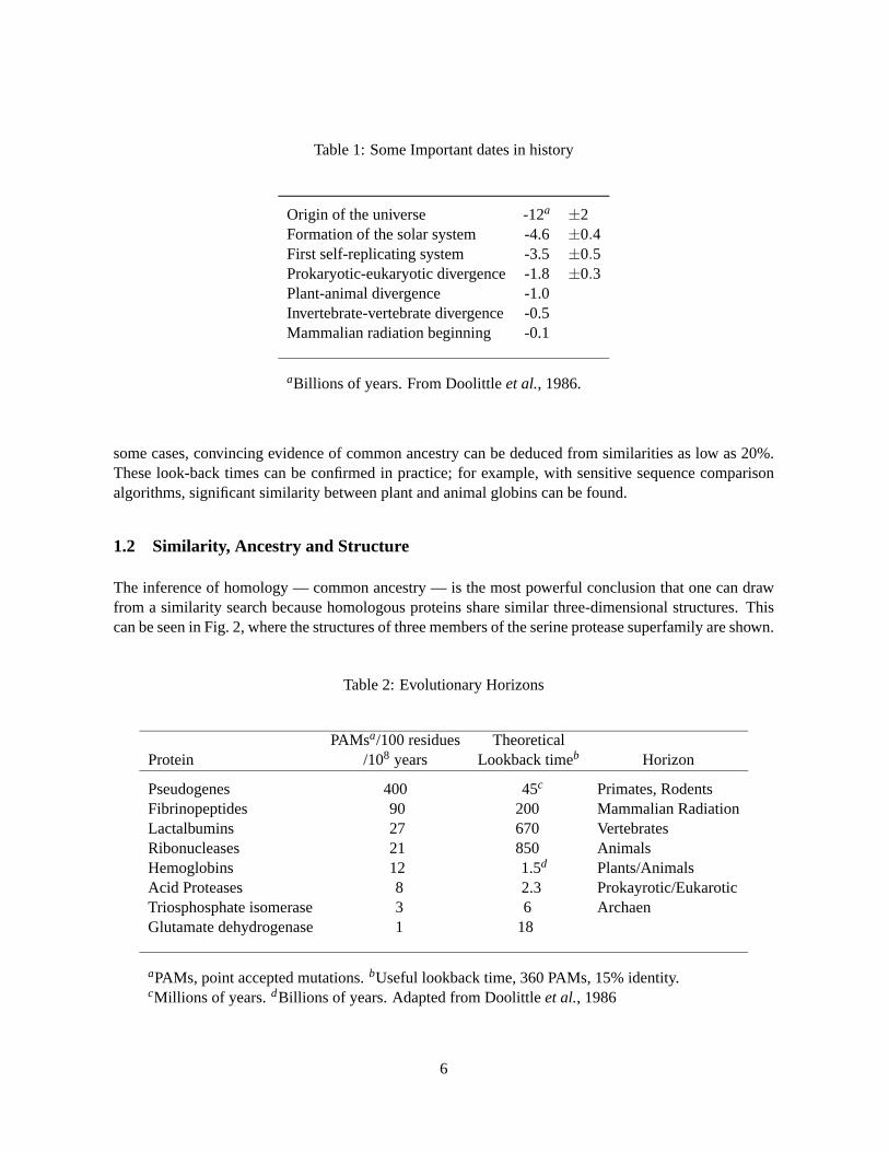
Table 1 summarizes some important milestones in evolutionary time, and, when considered withTable 2, gives a better perspective on the evolutionary horizons provided by different protein families.The theoretical lookback times in Table 2 are based on the assumption that one can identify proteins thatshare about 20% sequence identity throughout their entire length. It will be clear from later examplesthat if two protein sequences share 25% identity across their lengths, they are homologous, and that in
4
Figure 1: The tree of life
Human Horse Fish Insects Fungi Wheat E. coli
chemical evolution
prokaryotes/eukaryotes
plants/animals
-4.0
-3.0
-2.0
-1.0
-0.1
vertebrates/arthopods
self-replicating systems
Tim
e (b
illio
n ye
ars)
M. jann.
Adapted from Dayhoffet al., 1978.
5
Table 1: Some Important dates in history
Origin of the universe -12a ±2Formation of the solar system -4.6±0.4First self-replicating system -3.5±0.5Prokaryotic-eukaryotic divergence -1.8±0.3Plant-animal divergence -1.0Invertebrate-vertebrate divergence -0.5Mammalian radiation beginning -0.1
aBillions of years. From Doolittleet al., 1986.
some cases, convincing evidence of common ancestry can be deduced from similarities as low as 20%.These look-back times can be confirmed in practice; for example, with sensitive sequence comparisonalgorithms, significant similarity between plant and animal globins can be found.
1.2 Similarity, Ancestry and Structure
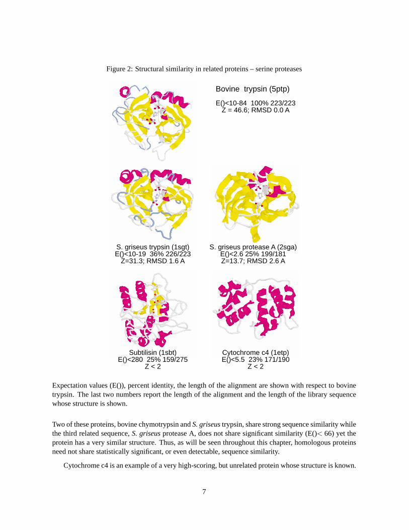
The inference of homology — common ancestry — is the most powerful conclusion that one can drawfrom a similarity search because homologous proteins share similar three-dimensional structures. Thiscan be seen in Fig. 2, where the structures of three members of the serine protease superfamily are shown.
Table 2: Evolutionary Horizons
PAMsa/100 residues TheoreticalProtein /108 years Lookback timeb Horizon
aPAMs, point accepted mutations.bUseful lookback time, 360 PAMs, 15% identity.cMillions of years.dBillions of years. Adapted from Doolittleet al., 1986
6
Figure 2: Structural similarity in related proteins – serine proteases
Bovine trypsin (5ptp)
E()<10-84 100% 223/223Z = 46.6; RMSD 0.0 A
S. griseus trypsin (1sgt)E()<10-19 36% 226/223
Z=31.3; RMSD 1.6 A
S. griseus protease A (2sga)E()<2.6 25% 199/181Z=13.7; RMSD 2.6 A
Subtilisin (1sbt)E()<280 25% 159/275
Z < 2
Cytochrome c4 (1etp)E()<5.5 23% 171/190
Z < 2
Expectation values (E()), percent identity, the length of the alignment are shown with respect to bovinetrypsin. The last two numbers report the length of the alignment and the length of the library sequencewhose structure is shown.
Two of these proteins, bovine chymotrypsin andS. griseustrypsin, share strong sequence similarity whilethe third related sequence,S. griseusprotease A, does not share significant similarity (E()< 66) yet theprotein has a very similar structure. Thus, as will be seen throughout this chapter, homologous proteinsneed not share statistically significant, or even detectable, sequence similarity.
Cytochrome c4 is an example of a very high-scoring, but unrelated protein whose structure is known.
7
This high scoring unrelated sequence does not share any structural similarity with trypsin or other serineproteases. If two proteins are not homologous, one cannot draw any conclusion about their structuralsimilarity, even though they may have high similarity scores.
1.3 Modes of Evolution
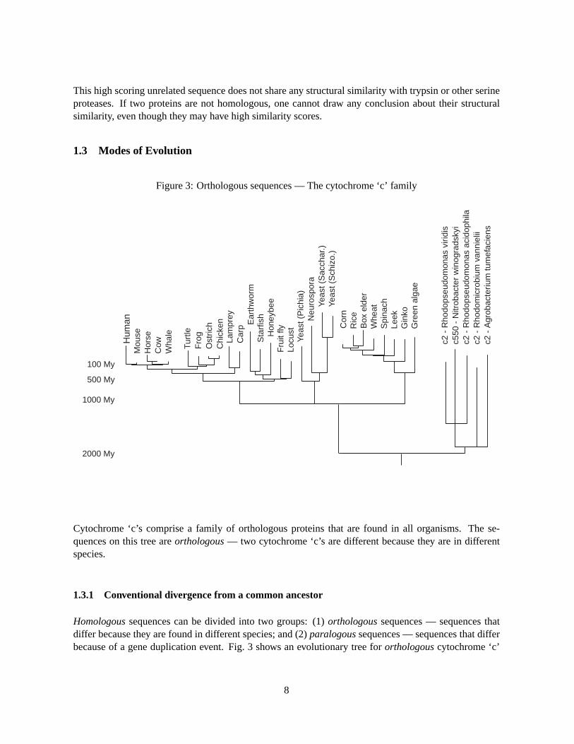
Figure 3: Orthologous sequences — The cytochrome ‘c’ family
Hum
anM
ouse
Hor
seC
owW
hale
Fro
gTu
rtle
Ost
rich
Chi
cken
Lam
prey
Car
p Ear
thw
orm
Sta
rfis
hH
oney
bee
Fru
it fly
Locu
stYe
ast (
Pic
hia)
Yeas
t (S
acch
ar.)
Yeas
t (S
chiz
o.)
Neu
rosp
ora
Cor
nR
ice
Box
eld
erW
heat
Spi
nach
Leek
Gin
koG
reen
alg
ae
c2 -
Rho
dops
eudo
mon
as v
iridi
sc5
50 -
Nitr
obac
ter
win
ogra
dsky
ic2
- R
hodo
pseu
dom
onas
aci
doph
ilac2
- R
hodo
mic
robi
um v
anni
elii
c2 -
Agr
obac
teriu
m tu
mef
acie
ns
100 My
500 My
1000 My
2000 My
Cytochrome ‘c’s comprise a family of orthologous proteins that are found in all organisms. The se-quences on this tree areorthologous— two cytochrome ‘c’s are different because they are in differentspecies.
1.3.1 Conventional divergence from a common ancestor
Homologoussequences can be divided into two groups: (1)orthologoussequences — sequences thatdiffer because they are found in different species; and (2)paralogoussequences — sequences that differbecause of a gene duplication event. Fig. 3 shows an evolutionary tree fororthologouscytochrome ‘c’
8
sequences. The branching pattern, which reflects the differences between cytochrome ‘c’ sequences,matches the evolutionary relationships of the species that express the proteins.
Figure 4: Orthology and paralogy — The globin family
β-glob
in - h
uman
myo
gobin
- wha
le
leghe
mog
lobin
δ-glob
in - h
uman
β-glob
in - m
ouse
β-glob
in - c
hicke
n
α-glob
in - c
himp.
α-glob
in - m
ouse
Members of the globin oxygen binding protein family have evolved through a series of gene duplicationsand speciation events. The humanα andδ genes duplicated less than 50 Mya (δ chains are found inprimates, but not in other mammals).
In general, the organismal tree and the sequence tree will not match if the sequences areparalogous.Members of the globin oxygen binding protein family are bothorthologous— they differ because ofspeciation — andparalogousp — they differ because of gene duplications. Thus, humanα-globin,mouseα-globin, and chickenα-globin are all orthologs, they differ because of the speciation eventsthat gave rise to humans, rodents, and birds. Mouseβ globin and humanα globin are paralogous; theydiffer because of a gene duplication that created theα and β subunits some 600 Mya (million yearsago). An evolutionary tree based on humanα, chickenα, and mouseβ would imply that humans aremore closely related to chickens than to mice. While such a mistake is unlikely in a well-studied familylike the globins, it can be quite common in large, diverse, and poorly characterized families like theG-protein-coupled receptors (Fig. 21).
9
1.3.2 Sequence similarity and homology, the H+ ATPase
Our first example of the significant sequence similarity shared by homologous proteins will use one ofthe chains of the H+-ATPase, or proton-pump, used to convert energy to ATP in the mitochrondria andchloroplasts of aerobic organisms.
The similarity scores in Figs. 6–8 were calculated using the Smith-Waterman algorithm (Smith &Waterman, 1981,Sec. 2.2), a method that guarantees to calculate the best (optimal) score between anytwo protein or DNA sequences, given a scoring matrix and gap penalties. Fig. 5 shows the PAM250matrix, which was developed almost 20 years ago by Dayhoff and her colleagues (Dayhoffet al., 1978).The PAM250 matrix, or modern versions such as the BLOSUM50 matrix used here, incorporates infor-mation about the likelihood that one amino-acid will be mutated into another over evolutionary time.Thus, changes that are very unlikely to occur in evolution, for example the substitution of the very smallglycine residue for the very large tryptophan residue, are given large negative scores (−7 in Fig. 5),while conservative changes, such as the substitution of lysine by arginine (both have basic side chains),are given positive scores (+3). The scores for identical matches also vary in the PAM250 matrix, de-pending on whether the amino-acids are common (e.g. serine and methionine), and thus likely to bealigned by chance, or rare (e.g. cysteine and tryptophan). There is a well-developed statistical theory forsubstitution matrices (Altschul, 1991), which will be discussed in section 3.2.
Table 3 reports similarity scores and their statistical significance from a search of the PIR annotatedprotein sequence database (PIR1, release 44, March, 1995) using the human H+-ATPase as a querysequence. There is excellent agreement between the expected and actual distributions of similarity scores.In this search, all of the library sequences related (homologous) to the query sequence obtained scoreshigher than any of the unrelated sequences. However, a number of unrelated sequences obtained very
10
Figure 6: Searching with human ATP-ase, similarity scores
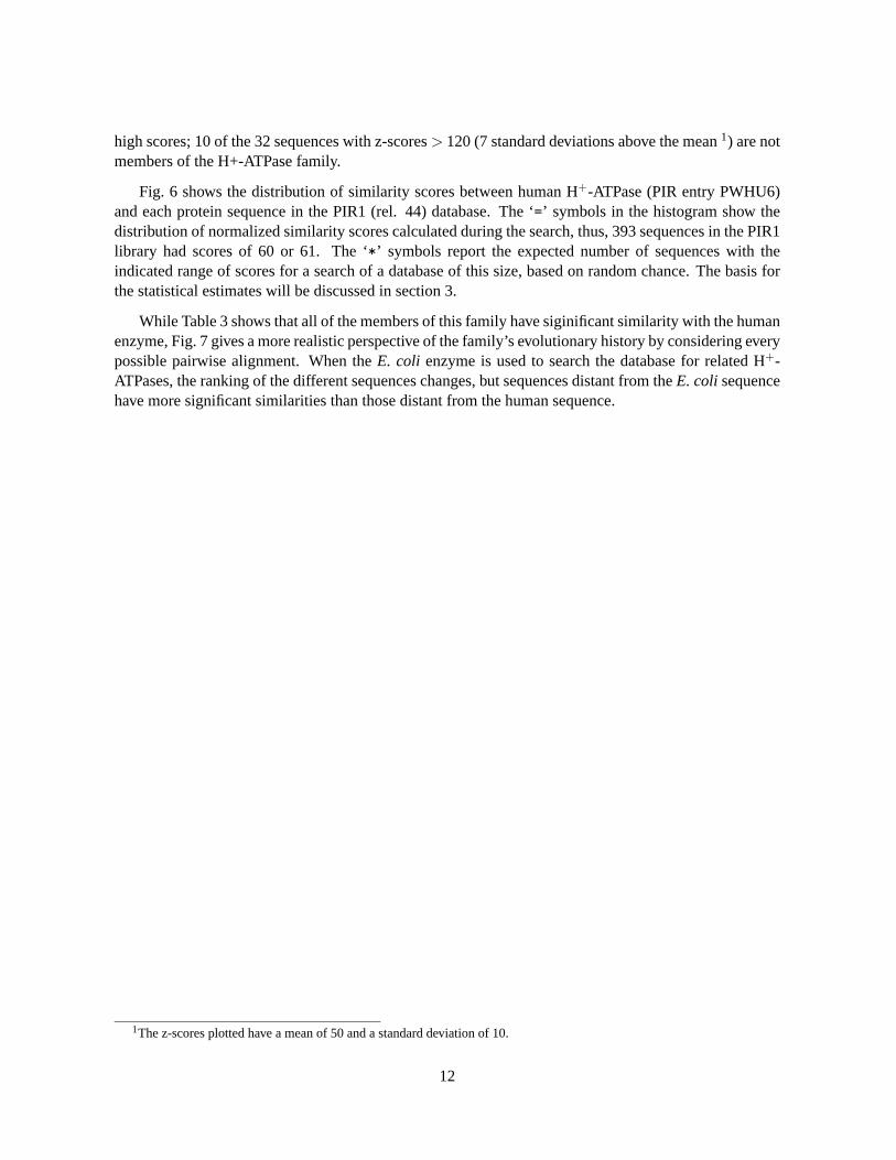
high scores; 10 of the 32 sequences with z-scores> 120 (7 standard deviations above the mean1) are notmembers of the H+-ATPase family.
Fig. 6 shows the distribution of similarity scores between human H+-ATPase (PIR entry PWHU6)and each protein sequence in the PIR1 (rel. 44) database. The ‘=’ symbols in the histogram show thedistribution of normalized similarity scores calculated during the search, thus, 393 sequences in the PIR1library had scores of 60 or 61. The ‘*’ symbols report the expected number of sequences with theindicated range of scores for a search of a database of this size, based on random chance. The basis forthe statistical estimates will be discussed in section 3.
While Table 3 shows that all of the members of this family have siginificant similarity with the humanenzyme, Fig. 7 gives a more realistic perspective of the family’s evolutionary history by considering everypossible pairwise alignment. When theE. coli enzyme is used to search the database for related H+-ATPases, the ranking of the different sequences changes, but sequences distant from theE. coli sequencehave more significant similarities than those distant from the human sequence.
1The z-scores plotted have a mean of 50 and a standard deviation of 10.
12
Table 3: Searching with human ATP-ase, high-scoring sequences
The best scores are: s-w bits E(14548) % len
PWHU6 H+-trans. ATP synth.—human mito. 1400 327 10−89 100.0 226PWBO6 H+-trans. ATP synth.—bovine mito. 1157 271 10−73 77.9 226PWMS6 H+-trans. ATP synth.—mouse mito. 1118 262 10−71 75.7 226PWXL6 H+-trans. ATP synth.—frog mito. 745 177 10−45 53.3 226PWFF6 H+-trans. ATP synth.—fruit fly mito. 471 115 10−26 37.5 224PWBY3 H+-trans. ATP synth.—yeast mito. 438 107 10−23 36.2 232PWAS6N H+-trans. ATP synth.—aspergillus mito. 365 91 10−18 30.4 230PWKQ6 H+-trans. ATP synth.—Cochliobolus mito. 353 88 10−17 31.3 214PWWT6 H+-trans. ATP synth.—wheat mito. 309 78 10−14 28.9 235PWNT6M H+-trans. ATP synth.—tobacco mito. 309 78 10−14 28.3 233PWZM6M H+-trans. ATP synth.—corn mito. 283 72 10−13 31.1 291LWEC6 H+-trans. ATP synth.—E. coli 178 48 10−5 23.3 236LWRZ6 H+-trans. ATP synth.—rice chloro. 144 40 0.00063 24.2 231PWPMA6 H+-trans. ATP synth.—pea chloro. 143 40 0.00074 25.0 232PWYBAA H+-trans. ATP synth.—Synechocystis 142 40 0.00099 26.5 170PWSPA6 H+-trans. ATP synth.—spinach chloro. 138 39 0.00016 24.2 231PWYCA6 H+-trans. ATP synth.—cyanobacteria 127 36 0.0099 26.3 167LWNT6 H+-trans. ATP synth.—tobacco chloro. 126 36 0.011 22.1 231LWLV6 H+-trans. ATP synth.—Marchiantia chloro. 126 36 0.011 24.0 167PWEGAC H+-trans. ATP synth.—Euglena chloro. 123 35 0.018 25.7 214
The horizontal line indicates the separation been the lowest scoring related sequences and the highestscoring unrelated sequence.
13
Figure 7: Phylogeny of H+-ATPases
Human mito.
Bovine mito.
Mouse mito.
Frog mito.
Fruit fly mito.
Yeast mito.
Cochliobolus mito.
Aspergillus mito.
Corn mito.
Wheat mito.
Rice chloro.
March. chloro.
Tobacco chloro.
Spinach chloro.
Pea chloro.
Cyanobacteria
Synechocystis
Euglena chloro.
E. coli
10-14/10-7
10-5/10-117
0.018/10-12
0.0002/10-12
0.0099/10-12
0.0010/10-11
0.011/10-12
0.0002/10-12
0.0007/10-11
0.011/10-11
10-23/10-7
10-26/0.007
10-89/10-6
10-17/10-5
10-18/10-6
10-13/10-8
10-73/10-5
10-71/10-5
10-45/10-6
An evolutionary tree of H+-ATPases (subunit 6). Sequences were aligned using the GCG PILEUP pro-gram, distances calculated using the GCG DISTANCES program, and the tree constructed using theNeighbor-Joining algorithm (GCG GROWTREE). Expectation values from a search with the humanH+-ATPase (PWHU6, Table 3) and a search with theE. coli sequence are shown.
14
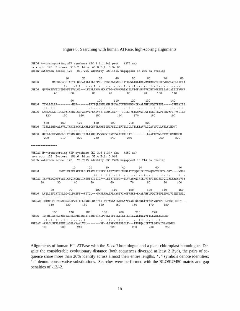
Figure 8: Searching with human ATPase, high-scoring alignments
LWEC6 H+-transporting ATP synthase (EC 3.6.1.34) prot (272 aa)
Alignments of human H+-ATPase with theE. coli homologue and a plant chloroplast homologue. De-spite the considerable evolutionary distance (both sequences diverged at least 2 Bya), the pairs of se-quence share more than 20% identity across almost their entire lengths. ‘:’ symbols denote identities;‘.’ denote conservative substitutions. Searches were performed with the BLOSUM50 matrix and gappenalties of -12/-2.
15
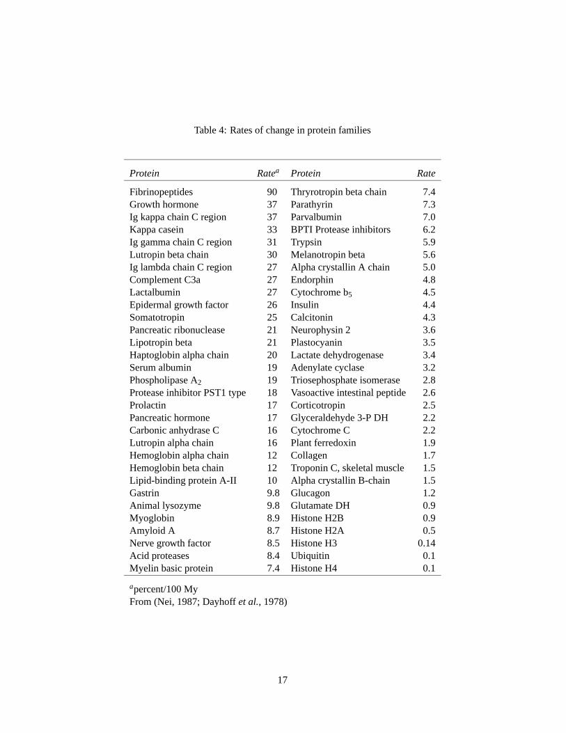
1.3.3 Protein families diverge at different rates
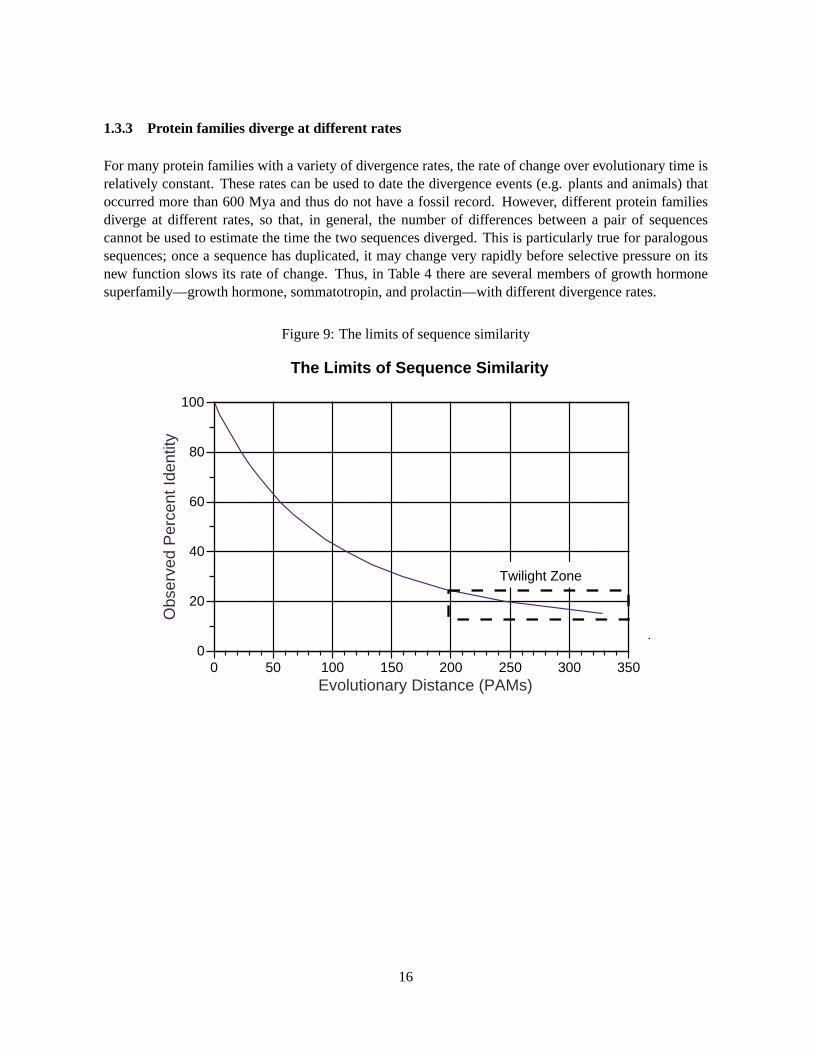
For many protein families with a variety of divergence rates, the rate of change over evolutionary time isrelatively constant. These rates can be used to date the divergence events (e.g. plants and animals) thatoccurred more than 600 Mya and thus do not have a fossil record. However, different protein familiesdiverge at different rates, so that, in general, the number of differences between a pair of sequencescannot be used to estimate the time the two sequences diverged. This is particularly true for paralogoussequences; once a sequence has duplicated, it may change very rapidly before selective pressure on itsnew function slows its rate of change. Thus, in Table 4 there are several members of growth hormonesuperfamily—growth hormone, sommatotropin, and prolactin—with different divergence rates.
“Conventional” protein families, e.g. the globins, cytochrome ‘c’s, H+-ATPases, in which protein se-quences have diverged from a common ancestor in a direct fashion, typically with only modest changesin the length of the sequence, have been known for more than 30 years. In the past 10 years, a morecomplex type of protein evolution has been observed—proteins that contain multiple domains from otherproteins. These proteins have been called “mosaic” proteins; the domains are frequently inserted througha process called “exon shuffling.” Table 7 lists a number of human proteins that are comprised of mosaicdomains, but such proteins are not limited to mammals. Similar mosaic structures are common in DNAbinding proteins, both in bacteria and eukaryotes.
Table 5: Classification of Protein Families
I. Ancient Proteins
A. First editions. Direct-line descendacy to human and contemporary prokaryotes. Mostly mainstreammetabolism enzymes. Example: triosphosphate isomerase (44.8% identical over 250 aa, E(59000)< 10−36).
B. Second edition. Homologous sequences in human and prokaryotic proteins, but apparently differentfunctions. Example: human glutathione reductase and pseudomonas mercury reductase (31% identi-cal over 438 aa, E(59000)< 10−32).
II. Middle-age proteins. Proteins found in most eukaryotes but prokaryotic counterparts are unknown. Exam-ple: actin (human and yeast share 88% identical over 375 aa, E()< 10−145, other yeast actin homologs shareas little as little as 26.4 % over 489 aa, E()< 10−14.
III. Modern proteins
A. Recent vintage. Proteins found in animals or plants but not both. Not found in prokaryotes. Example:collagen.
B. Very recent inventions. Proteins found in vertebrates but not elsewhere. Example: plasma albumin.
C. Recent mosaics. Modern proteins clearly the result of exon shuffling. Example: LDL receptor.
From Doolittleet al., 1986.
1.4 Introns Early/Late
The occurrence of mosaic proteins and the discovery of the “exon/intron” structure of genes in the late1970’s led several investigators to suggest that the exon structure of genes reflected the construction ofproteins from modular domains (Gilbert & Glynias, 1993). While acceptance of this proposal is quitewidespread, it is based on very little data. There is no question that many modern mosaic proteins areconstructed by a process of “exon-shuffling” whereby exons from other genes have been combined tobuild new structures. In addition, for some proteins exons are associated with well defined structural
18
Table 6: Ancient human proteins
A. First edition type
Human protein Prokaryotic homologue % identity E(59,000)
elements. The association of exons with structural elements may reflect and ancient construction ofproteins from primordial exons. Alternatively, introns are also capable of invading genes; thus, theassociation of exons with structures may reflect modern invasions that are less disruptive when theyoccur between structural elements.
A recent test of the “introns” early hypothesis suggests there is little evidence to support the associa-tion of introns with structural boundaries (Stoltzfuset al., 1994.
1.5 DNA vs Protein comparison
While all of the comparison methods described below work on either protein or DNA sequences, one’sability to identify distantly related sequences is reduced dramatically when DNA sequences are used.Fig. 8 compares the statistical significance of the best similarity scores obtained in a search of the Gen-Bank DNA sequence database using a mouse glutathione transferase cDNA clone with the significanceof the same alignment in a search of the GenPept protein sequence database (GenPept is derived fromGenBank by translating DNA sequences into the encoded protein sequences). Many DNA sequencesencoding clearly related proteins, e.g. RABGSTB have similarity scores that are expected to occur sev-eral times by chance in a DNA database search. DNA sequences are far less informative, both becausethey lack the inherent biochemical information that is retained in the PAM250 substitution matrix, andbecause many changes in DNA sequences (third-base changes) do not change the encoded protein.
Differences in the performance of sequence comparison algorithms are insignificant compared to theloss of information that occurs when one compares DNA sequences. If the biological sequence of interest
19
Table 7: Mosaic proteins
A. EGF-type B. C9-typeEpidermal growth factor precursor Complement C9Tumor growth factors LDL receptorLDL receptor Notch (Drosophila)Factor IX lin-12 (C. elegans)Protein CTissue plasminogen activator C. Fibronectin fingerUrokinase FibronectinComplement C9 Tissue plasminogen activatorNotch protein (Drosophila)lin-12 (C. elegans) D. Protease “Kringle”
Expectation values for searches against DNA (score, E(DNA)), protein (E(prot)), and translated DNA (E(tx)databases. A mouse glutathione transferase cDNA sequence (MUSGST) was used to search either the primate(GBPRI), rodent (GBROD), and mammalian (GBMAM) divisions of the GenBank DNA sequence database forthe DNA sequence comparisons. Protein expectations (E(prot)) were calculated from a search the translated cDNAsequence against the GenPept sequence database, which includes all of translated GenBank. Unrelated sequencesareitalicized; E(prot) for unrelated sequences are>> 100.
21
2 Alignment methods
A variety of comparison algorithms and scoring parameters can be used to evaluate protein or DNAsequence similarity. In general, the choice the of “best” algorithm depends on the problem to be solved.Thus, algorithms that calculate a local comparison score—i.e., they find the strongest similarity betweenthe two sequences, ignoring differences outside of the most similar region—are usually most appropriatefor searching protein and DNA databases,2 while global comparison algorithms are more appropriatewhen homology has been established, as when building evolutionary trees. Pattern-based, rather thansimilarity-based, comparison methods may be preferred when searching for functionally conserved non-homologous domains.
In searching protein sequence databases to identify distantly related homologous proteins, it is im-portant to remember that avoiding high similarity scores with unrelated sequences can be more importantas calculating high scores for related sequences. There are more than 50,000 protein sequences in com-prehensive protein databases, while the typical family of proteins has fewer than 100 members. Thus,comparison algorithms, scoring matrices and gap penalties that produce the best alignments may not bethe most effective for searching protein sequence databases (Pearson, 1995; Pearson, 1998).
2.1 Algorithms
Two general classes of comparison algorithms are used to calculate similarity scores to infer sequencehomology: rigorous algorithms that are guaranteed to calculate an optimal similarity score, e.g. theNeedlemanWunsch (Needleman & Wunsch, 1970) and SmithWaterman (Smith & Waterman, 1981) al-gorithms, and rapid heuristic algorithms that do not guarantee to calculate an optimal score for everysequence in a library, e.g. FASTA (Pearson & Lipman, 1988) and BLAST(Altschulet al., 1990). Ta-ble 2.1 summarizes widely used algorithms for biological sequence comparison.
Two optimal algorithms for calculating similarity scores have been described, the NeedlemanWunschalgorithm (Needleman & Wunsch, 1970), which calculates a “global” similarity score between two se-quences, and the Smith-Waterman algorithm (Smith & Waterman, 1981), which calculates a “local”similarity score. Global scores require the alignment to begin at the beginning of each sequence andextend to the end of each sequence. Global alignments cannot be used to detect the relationship betweenDNA binding domains in homeobox proteins or the calcium binding domains shared between calmodulinand calpain. Likewise, global alignment algorithms often do not detect the relationships between mosaicproteins. Global similarity scores can be calculated with or without penalties for gaps at the ends of thesequences.
Local alignment algorithms identify the most similar region shared between two sequences. Thus,homologous calcium binding domains embedded in non-homologous proteins can be detected with localalignment methods. In addition, a local alignment algorithm can be used to find the exons in a genomicDNA sequence by aligning it with its encoded mRNA. Local alignment algorithms are required to identifyhomologies in mosaic proteins, and they can be used to detect internal domain duplications as well.Table 10 compares the scores of global, global without end-gap-penalties, and local similarity scores for
2For genomic DNA sequences, there is no logical alternative.
22
Table 9: Algorithms for comparing protein and DNA sequences
algorithm value scoring gap timecalculated matrix penalty required
Smith- local similarity Si j < 0.0 affine O(n2) Smith and Waterman, 1981Waterman q+ rk Gotoh, 1982
FASTA approx. local Si j < 0.0 limited gap size O(n2)/K Lipman and Pearson, 1985similarity q+ rk Pearson and Lipman, 1988
BLASTP maximum Si j < 0.0 multiple O(n2)/K Altshul et al., 1990segment score segments
a variety of related and unrelated proteins.
Rigorous sequence comparison algorithms, like the Smith-Waterman algorithm, require time propor-tional to O(mN), wherem is the length of the query sequence andN is the number of amino acids inthe protein sequence library. Modern high-performance unix workstations can compare a 300 residueprotein sequence (human opsin) to the 40,000 entry, 15,000,000 amino acid Swiss-Prot 31 database inless than 10 minutes.
Although very rapid3 algorithms are available for calculating optimal global similarity scores be-tween two sequences, particularly with unit cost scores, such algorithms are rarely appropriate for bio-logical sequence comparison. Unit cost algorithms must discard the substantial biochemical informationencoded in the PAM250 matrix. Most rapid optimal algorithms calculate only global similarities; suchcomparisons are not useful for DNA sequence comparison because the “ends” required for a global se-quence comparison are usually arbitrary.
2O(Nd), whereN is the length of a sequence andd is the number of differences between the two sequences.
23
Table 10: Global and local sequence similarity scores
The algorithms used to calculate the maximum similarity scores between two sequences are most easilyvisualized with an alignment matrix or path graph. Figs. 10–11 demonstrate the correspondence betweenan alignment path graph and an actual alignment. The goal along the path is to maximize the similarityscore for the alignment that ends at each potential vertex. For the figures, similarity scores are increasedby +1 for diagonal edges if the two residues along the path are identical; if they are different, the diagonaledge cost is−1. The cost along either a horizontal or vertical edge, which corresponds to an insertionin the top sequence (horizonal edge) or an insertion in the left-side sequence (vertical edge) is−2. Toproduce a global alignment from a path graph, simply begin at the bottom-right corner of the graph andfollow the “active” paths, noted by\, or ! to the upper-left corner, aligning the two residues along thediagonal path, or aligning a residue with a gap if a horizontal or vertical path is taken.
For the global alignment in Fig. 10A, there are two alignments that produce the optimal score. Op-timal comparison algorithms guarantee to produce the best score, given the match, mismatch, and gapcosts, but frequently there are several optimal alignments for a single score. For the local alignment inFig. 10B, there are several sub-optimal alignments with scores of 2. Note that the local alignment inFig. 10B would extend from one end of each sequence to the other if the gap cost were reduced to−1.
Fig. 11 provides an exercise for the reader.
While there are an exponential number of potential alignments with gaps between two protein or
25
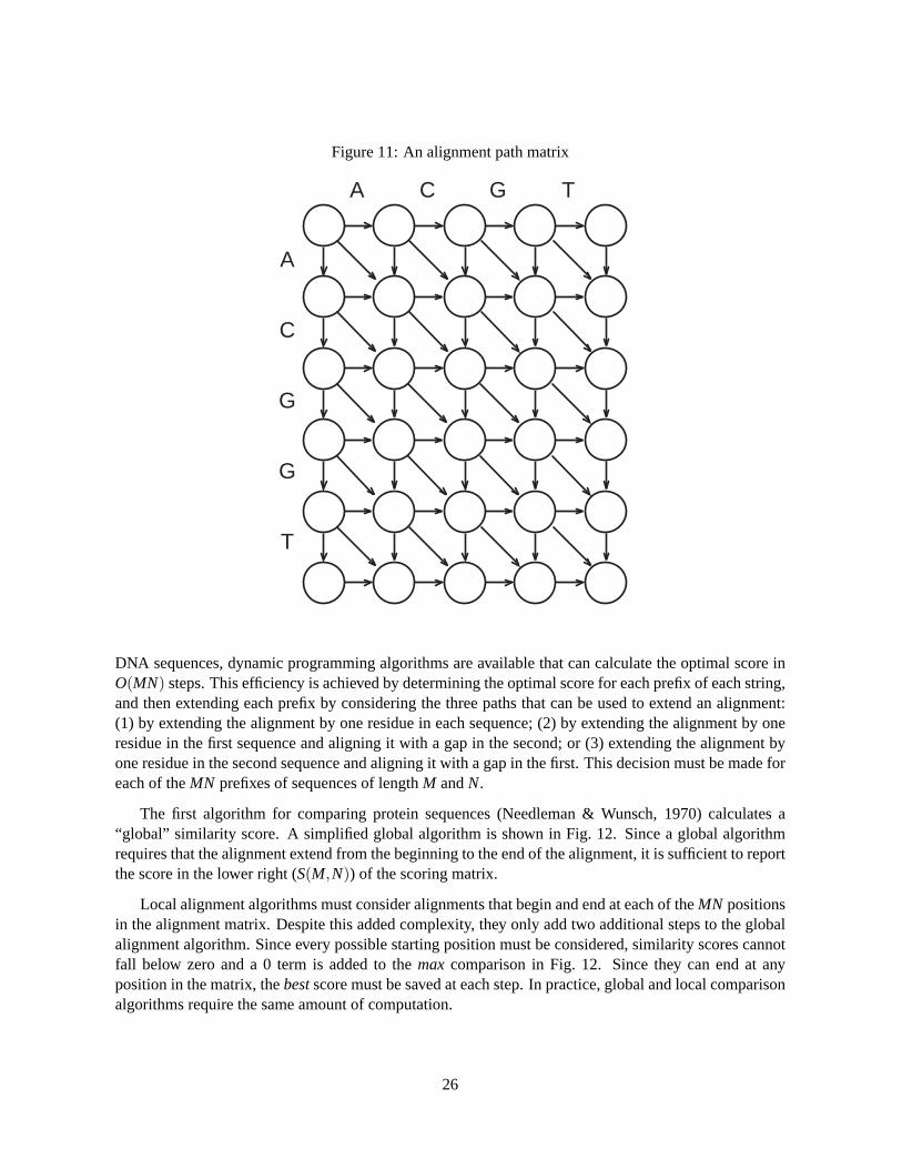
Figure 11: An alignment path matrix
A C G T
A
C
G
G
T
DNA sequences, dynamic programming algorithms are available that can calculate the optimal score inO(MN) steps. This efficiency is achieved by determining the optimal score for each prefix of each string,and then extending each prefix by considering the three paths that can be used to extend an alignment:(1) by extending the alignment by one residue in each sequence; (2) by extending the alignment by oneresidue in the first sequence and aligning it with a gap in the second; or (3) extending the alignment byone residue in the second sequence and aligning it with a gap in the first. This decision must be made foreach of theMN prefixes of sequences of lengthM andN.
The first algorithm for comparing protein sequences (Needleman & Wunsch, 1970) calculates a“global” similarity score. A simplified global algorithm is shown in Fig. 12. Since a global algorithmrequires that the alignment extend from the beginning to the end of the alignment, it is sufficient to reportthe score in the lower right (S(M,N)) of the scoring matrix.
Local alignment algorithms must consider alignments that begin and end at each of theMN positionsin the alignment matrix. Despite this added complexity, they only add two additional steps to the globalalignment algorithm. Since every possible starting position must be considered, similarity scores cannotfall below zero and a 0 term is added to themax comparison in Fig. 12. Since they can end at anyposition in the matrix, thebestscore must be saved at each step. In practice, global and local comparisonalgorithms require the same amount of computation.
26
Figure 12: Algorithms for Global and Local similarity scores
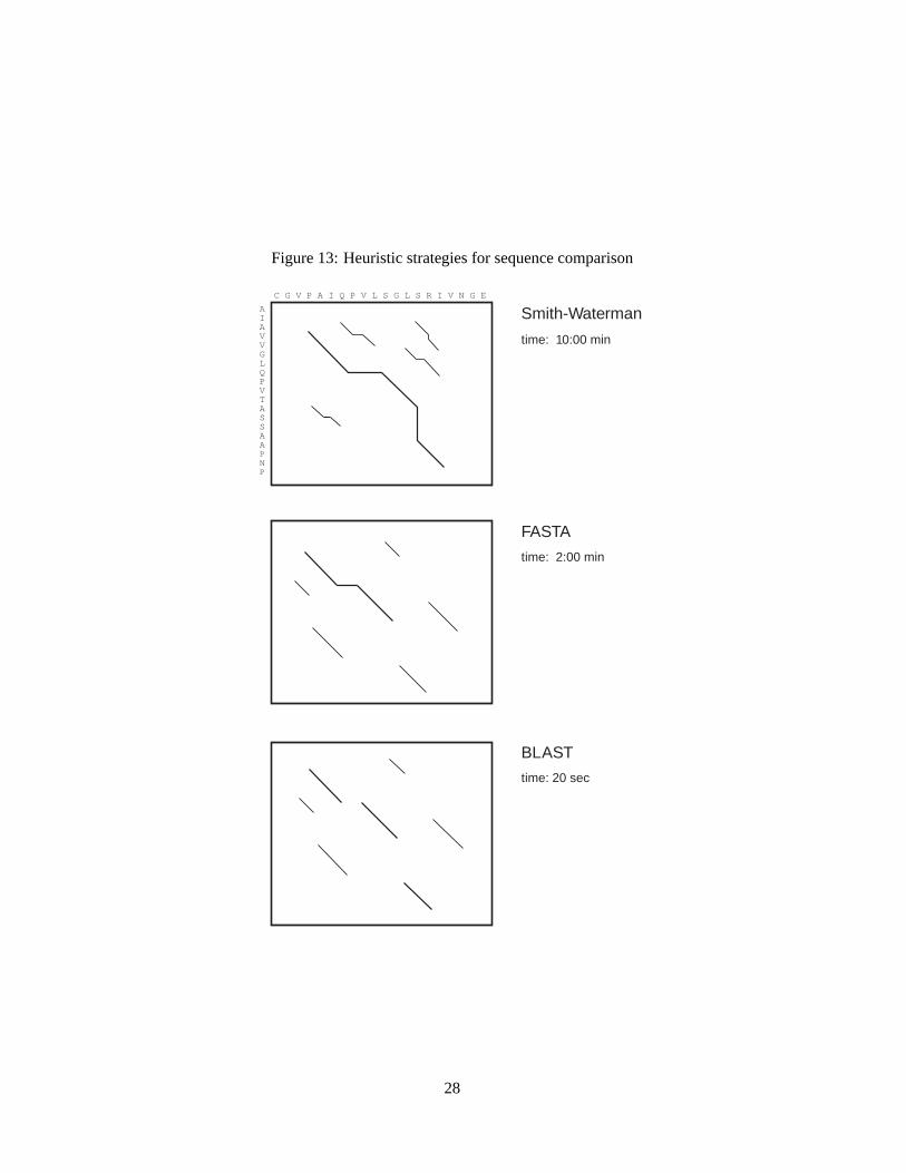
Two rapid heuristic algorithms are frequently used for searching protein and DNA sequence databases,FASTA (Pearson & Lipman, 1988) and BLASTP (Altschulet al., 1990). These methods are 5–50 timesfaster than the rigorous Smith-Waterman algorithm, and can produce results of similar quality in manycases.
Fig. 13 summarizes the difference between the FASTA, BLASTP, and Smith-Waterman algorithms.BLASTP and FASTA are faster than Smith-Waterman because they examine only a portion of the poten-tial alignments between two sequences. FASTA focuses on regions where there are either pairs (ktup=2)or single alignedktup=1 identities; BLASTP examines regions that include triples of conserved aminoacids.
27
Figure 13: Heuristic strategies for sequence comparison
C G V P A I Q P V L S G L S R I V N G E
Smith-WatermanAIAVVGLQPVTASSAAPNP
FASTA
BLAST
time: 10:00 min
time: 2:00 min
time: 20 sec
28
Table 11: Sequence similarity with BLASTP
Step 1 For each three amino acids in the query sequence, identify all of the substitutions of each word that have asimilarity score greater than a threshold scoreT =. In practice, word-matches with scores≥ T are seen onaverage 150 times per library sequence.
Step 2 Build a discrete finite automaton (DFA) to recognize the list of identical and substituted three letter words.
Step 3 Use the DFA to identify all of the matching words in sequences in the database. If two matches are found,extend each match both forwards and backwards using the BLOSUM62 matrix, allowing gaps, to produce ascore that is higher than a threshold score. Save all of the high scoring regions shared by the query sequenceand each library sequence.
Step 4 Report all of the significant alignments. Frequently, a query and library sequence will contain several MSPsbecause of the requirement that they do not contain gaps.
2.3.1 BLAST
Advances in the statistical theory of sequence alignments without gaps (Karlin & Altschul, 1990) pro-vided the theoretical basis for the BLASTP program (Altschulet al., 1990). BLASTP is now the mostwidely used program for rapid sequence comparison, in large part because of its accurate estimates forthe statistical significance of similarity scores (see 3. BLASTP, like FASTA, uses a word-based scanningprocedure to identify regions of local similarity (Table 11) with out gaps. BLASTP is effective becauseit combines high sensitivity with excellent selectivity. BLASTP combines good sensitivity with excep-tional selectivity. Except when the query sequence contains a low complexity region, BLASTP rarelycalculates scores for unrelated sequences.
2.3.2 FASTA
The current version of FASTA provides several significant improvements over earlier versions. FASTAnow calculates optimized scores (step 4 in Table 12)) for most of the sequences in the database andprovides accurate estimates for statistical significance (3). Calculation of optimized scores improvessubstantially the performance of FASTA. Without the calculation, FASTA performs significantly worsethan BLASTP; however, with the calculation of optimized scores (and normalization of the scores basedon library sequence length), FASTA performs significantly better than BLASTPv1.4 and almost as wellas the Smith-Waterman algorithm (Pearson, 1995). In addition, FASTA now uses the Smith-Watermanalgorithm to produce final alignments; previous versions limited the size of gaps, which sometimes ledto incomplete alignments.
Every database search for members of a diverse protein family involves a tradeoff between sensitivity—the ability to identify distantly related members of the family—and selectivity—the ability to avoid highsimilarity scores for unrelated sequences. Table 3.3 compares how effectively the three algorithms main-tain this balance for a large protein family—the G-protein-coupled receptors. Thus, BLASTP calculatesa very highly significant score for the closely related opsin and dopamine D2 receptors, and a significantscore for the more distantly related thromboxane A2 receptor, but it does not detect the similarity between
29
Table 12: Sequence similarity with FASTAv33
Step 1 Identify regions shared by the two sequences with the highest density of identities (ktup=1) or pairs ofidentities (ktup=2). If the -S option is used, low-complexity (lower-case) letters are ignored in steps 1–5.
Step 2 Rescan the ten regions with the highest density of identities using the BLOSUM50 matrix. Trim the ends ofthe region to include only those residues contributing to the highest score. Each region is a partial alignmentwithout gaps.
Step 3 If there are several initial regions with scores greater than the CUTOFF value, check to see whether thetrimmed initial regions can be joined to form an approximate alignment with gaps. Calculate a similarityscore that is the sum of the joined initial regions minus a penalty (usually 20) for each gap (initn). The scoreof the single best initial region found in Step 2 is also reported (init1).
Step 4 For sequences with scores greater than a threshold, construct an optimal local alignment of the query se-quence and the library sequence, considering only those residues that lie in a band centered on the bestinitial region found in Step 2. For protein searches withktup=2a 16 residue band is used by default. A 32residue band is used withktup=1. This is the optimized (opt) score.
Step 5 (Statistical estimates) After the first 60,000 scores have been calculated, normalize the raw similarity scoresusing estimates for the statistical parameters of the extreme value distribution. The default strategy regressesthe similarity score against ln(library-sequence length) and calculating the average variance in similarityscores. Z-values(normalized scores with mean 0 and variance 1) are calculated, and the calculation isrepeated with library sequences withz-valuesgreater than 5.0 and less than -5.0 removed. These z-valuesare used to rank the library sequences, but other estimation strategies are available.
Step 6 The Smith-Waterman algorithm (without limitation on gap size) is used to display alignments. Final align-ments score low-complexity regions.
opsin and the very distantly relatedDictyosteliumcAMP (CAR1) receptor. In addition, BLASTP wouldnever suggest a relationship between opsin and cytochrome oxidase. FASTA (ktup=2 does a better jobat recognizing the relationship between opsin and thromboxane A2, fails to detect the cAMP-1 receptor,and is more ambiguous about a possible relationship with cytochrome oxidase. FASTA withktup=1and Smith-Waterman calculate statistically significant relationships between opsin and cAMP-1, but alsogood (but not significant) scores for opsin and cytochrome oxidase.
3 The statistics of sequence similarity scores
The development of accurate statistical estimates for local sequence similarity scores (Karlin & Altschul,1990; Mott, 1992) has allowed dramatic improvement in our ability to reliably recognize distantly re-lated proteins. The statistical estimates calculated by BLASTP are used widely in large scale sequencecomparison, e.g. to characterize all of the genes on a yeast chromosome or all of the genes in a bacte-rial genome. The incorporation of statistical estimates into FASTA and SSEARCH (a Smith-Watermanimplementation) have significantly improved the performance of these programs as well.
30
Figure 14: The extreme value distribution
0
2000
4000
6000
8000
10000
-2.0 0.0 2.0 4.0 6.0
-2.0 0.0 2.0 4.0 6.0 8.0
14 16 18 20 22 24 26 28 30
z(σ)
λS
bit
num
ber
of s
eque
nces
similarity score
3.1 Sequence alignments without gaps
The statistics of local similarity scores for alignments without gaps but with an arbitrary substitutionmatrix have been described by Karlin & Altschul, 1990. Local similarity scores are described by theextreme valuedistribution. Using the parametersλ andK, which can be derived from the scoring matrixand the amino acid composition of the query sequence, the probability that a normalized similarity score:
S′ = λS− lnKmn (1)
(Karlin & Altschul, 1990; Altschulet al., 1994) wherem is the length of the query sequence andn is thelength of the library sequence can be calculated as:
P(S′ ≥ x) = 1−exp(−e−x) (2)
orP(S≥ x) = 1−exp(−Kmne−λx) (3)
Since a typical database search typically involves thousands of pairwise comparisons, the expectationof finding a scoreS′ ≥ X for a search ofD sequences is:E(S′ ≥ X) = PD. (Thus, searches of highlyredundant databases may be less informative, becauseD is larger but the number of different sequencesis not.)
3.2 Scoring matrices
The scoring matrices used for protein sequence comparison are much more sophisticated than+1 fora match and−1 for a mismatch. The most effective matrices are based on the actual frequency of
31
substitutions that occur between related proteins. Similarity scoring matrices can differ in three ways:(1) the method by which they are constructed; (2) their information content, which is related to thenumber of residues that must be aligned to produce a statistically significant score, and (3) their scale -the amount of information provided per unit score.
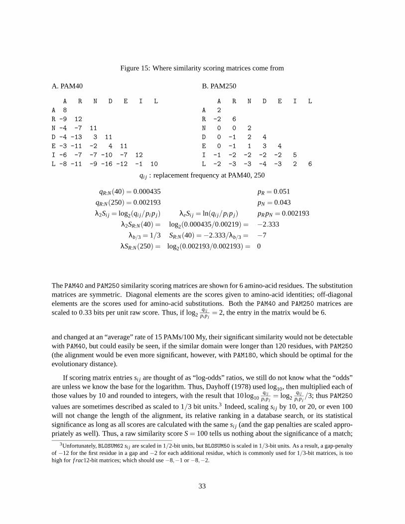
Two general approaches have been used to produce scoring matrices. The original PAM250 matrix(Fig. 5) was produced by examining several hundred alignments between very closely related proteins,and then calculating the frequency with which each amino-acid residue changed into each of the oth-ers at a very short evolutionary distance—one where only 1% of the residues had kchanged (Dayhoffet al., 1978). This replacement frequency, when corrected for the amino-acid abundance, can be usedto calculate the PAM1 scoring matrix (PAM is “Point Accepted Mutation”). If the matrix is multipliedagainst itself 250 times, a PAM250 matrix, which reflects the frequency of change for proteins that havediverged 250%. If two protein sequences have diverged by 250%, it is expected that they will share about20% sequence identity (Fig. 9). Since 20% identity is at the edge of where significant similarity can bedetected, the PAM250 matrix has been widely used. The PAM250 matrix is based on small number ofamino acid substitutions; modern extrapolated matrices based both on sequence alignments (Joneset al.,1992) and structural alignments (Johnson & Overington, 1993) are available.
Alternatively, substitution matrices can calculated directly by examining “blocks” of aligned se-quences that differ by no more thanX% (Henikoff & Henikoff, 1992). Thus, the BLOSUM62 matrix,which is used by the BLASTP rapid comparison program, is derived from substitution data for blocks ofaligned sequences that are no more than 62% identical. BLOSUM62 performs substantially better thanextrapolated matrices with BLASTP and FASTA (Henikoff & Henikoff, 1993), but both BLOSUM andextrapolated matrices can perform well when used with optimal gap penalties (Pearson, 1995).
PAM-style matrices and BLOSUM matrices differ not only in the way they they are built, but also inthe way they are used. “Shallow” PAM matrices (PAM20, PAM20, PAM40) have low numbers, and indicatethat very little evolutionary change has taken place. “Conservative” BLOSUM matrices (e.g.BLOSUM80)have high numbers, and indicate a high degree of sequence conservation, in contrast to a small amountof evolutionary change.
Altschul (1991) has provided a information-theory based perspective for evaluating scoring matricesin general for alignments without gaps (Altschul, 1991). With this interpretation, one can think of eachentry si j in a scoring matrix as a “log-odds” valuesi j = log( qi j
pi p j), whereqi j is the “target” residue
substitution frequency—the frequency with which residueA is replaced byM, or vice-versa, after a certainamount of evolutionary change—andpi , p j are the probabilities that the residues would align by chance,based solely on their frequency in a sequence. For a given pairwise sequence comparison,pi , p j willremain the same for scoring matrices at different evolutionary distances, butqi j will vary, depending onhow much change is expected. Thus, in Fig. 15, thePAM40 matrix gives much larger positive scores foridentical matches, lower negative scores for non-conservative replacements, and gives some replacementsnegative scores that are scored as conservative replacements whenPAM250 is used. In addition, onecan calculate the the average score, information content, or relative entropyH, that is expected peraligned residue:H = λ∑i j qi j si j = ∑i j qi j log2
qi j
pi p jif λsi j is scaled in bits. For thePAM40 andPAM250
matrices in Fig 15,H = 2.26 andH = 0.354 bits/residue. If 40 bits of information are required to obtainan expectation valueE(80,000) < 0.001, then an alignment of only 40/2.26 = 18 residues would berequired on average forPAM40, while 113 residues would be required withPAM250. However, if the twosequences last shared a common ancestor 600 Mya, and thus the sequences are separated by 1200 My,
32
Figure 15: Where similarity scoring matrices come from
A. PAM40
A R N D E I LA 8R -9 12N -4 -7 11D -4 -13 3 11E -3 -11 -2 4 11I -6 -7 -7 -10 -7 12L -8 -11 -9 -16 -12 -1 10
B. PAM250
A R N D E I LA 2R -2 6N 0 0 2D 0 -1 2 4E 0 -1 1 3 4I -1 -2 -2 -2 -2 5L -2 -3 -3 -4 -3 2 6
qi j : replacement frequency at PAM40, 250
qR:N(40) = 0.000435 pR = 0.051
qR:N(250) = 0.002193 pN = 0.043
λ2Si j = log2(qi j/pi p j) λeSi j = ln(qi j/pi p j) pRpN = 0.002193
λ2SR:N(40) = log2(0.000435/0.00219) = −2.333
λb/3 = 1/3 SR:N(40) =−2.333/λb/3 = −7
λSR:N(250) = log2(0.002193/0.002193) = 0
ThePAM40 andPAM250 similarity scoring matrices are shown for 6 amino-acid residues. The substitutionmatrices are symmetric. Diagonal elements are the scores given to amino-acid identities; off-diagonalelements are the scores used for amino-acid substitutions. Both thePAM40 andPAM250 matrices arescaled to 0.33 bits per unit raw score. Thus, if log2
qi j
pi p j= 2, the entry in the matrix would be 6.
and changed at an “average” rate of 15 PAMs/100 My, their significant similarity would not be detectablewith PAM40, but could easily be seen, if the similar domain were longer than 120 residues, withPAM250(the alignment would be even more significant, however, withPAM180, which should be optimal for theevolutionary distance).
If scoring matrix entriessi j are thought of as “log-odds” ratios, we still do not know what the “odds”are unless we know the base for the logarithm. Thus, Dayhoff (1978) used log10, then multiplied each ofthose values by 10 and rounded to integers, with the result that 10 log10
qi j
pi p j= log2
qi j
pi p j/3; thusPAM250
values are sometimes described as scaled to 1/3 bit units.3 Indeed, scalingsi j by 10, or 20, or even 100will not change the length of the alignment, its relative ranking in a database search, or its statisticalsignificance as long as all scores are calculated with the samesi j (and the gap penalties are scaled appro-priately as well). Thus, a raw similarity scoreS= 100 tells us nothing about the significance of a match;
3Unfortunately,BLOSUM62 si j are scaled in 1/2-bit units, butBLOSUM50 is scaled in 1/3-bit units. As a result, a gap-penaltyof −12 for the first residue in a gap and−2 for each additional residue, which is commonly used for 1/3-bit matrices, is toohigh for f rac12-bit matrices; which should use−8,−1 or−8,−2.
33
Figure 16: Similarity scores and library sequence length
0
25
50
75
100
125
150
10 100 1000 10000
sim
ilarit
y sc
ore
sequence length
unrelated related
regression-scaled
0
25
50
75
100
125
150
10 100 1000 10000
sim
ilarit
y sc
ore
sequence length
unrelated related
0
25
50
75
100
125
150
10 100 1000 10000
sim
ilarit
y sc
ore
sequence length
0
25
50
75
100
125
150
10 100 1000 10000
sim
ilarit
y sc
ore
sequence length
Glutathione transferase
Opsin OOHU
unscaled scores
The distribution of Smith-Waterman similarity scores is plotted as a function of log(n), n is the length ofthe library sequence. Filled symbols indicate individual related sequences (only the most distant relatedsequences are shown); open symbols show the average and std. error of similarity scores for unrelatedsequences.
one must also know the scoring matrix and its “scale”, or, more specifically, itsλ, or describe the score interms of the number of standard deviations above the mean for sequences of that size. Current versionsof theblast2 andfasta3 programs report scores in terms ofbits, whereoSbit = (λSraw− lnK)/ ln2.Thus, substituting in equation 3:
E(Sbit) = mn2−Sbit =mn2Sbit
(4)
For ungapped alignments,λ andK can be calculated analytically (Karlin & Altschul, 1990). For align-ments with gaps, they must be estimated.
34
Table 13: Search Algorithms and Statistical Significance
algorithm closely related distantly unrelatedrelated related
Expected number of times that a similarity score as high or higher than that obtained by the indicatedlibrary sequence would be obtained by chance in a search of Swiss-Prot (≈ 100,000 entries) with theOPSDHUMAN (human opsin) query sequence.eExpected times this score would be obtained after100,000 shuffles of the indicated library sequence with either global (prss) or local (window=20) aminoacid exchanges.
3.3 Empirical statistics for alignments with gaps
The normalization in equation 1 shows that scores for alignments without gaps between random se-quences increase as lnKmn, or sinceK andm are fixed for a given search, lnn, the length of the librarysequence. This is seen empirically with scores for alignments that contain gaps (Collinset al., 1988;Mott, 1992) and is shown in Fig. 16. For local similarities, the variance of the score should be in-dependent of library sequence length. Thus, normalization of similarity scores by fitting a line to therelationship of similarity score to lnn will reduce the scores of long, unrelated sequences, and make itpossible to detect more distant relationships (Pearson, 1995).
Accurate statistical estimates for alignments with gaps can can be calculated by normalizing simi-larity scores to remove the lnn dependence for similarity scores. This can be seen in Fig. 6, where the‘*’s show the fit of an extreme value distribution to the observed data (‘==’). FASTA and SSEARCHestimate statistical significance by fitting a line toSvs lnn and calculating the average variance for thescores. The regression line and variance are used to calculate
Z−score= (S− (a+blnn))/√
var (5)
The distribution ofZ−score’s should follow the extreme value distribution, so that:
P(Z> x) = 1−exp(−e−1.282Z−0.5772) (6)
and, as before,E(Z> x) = PD.
35
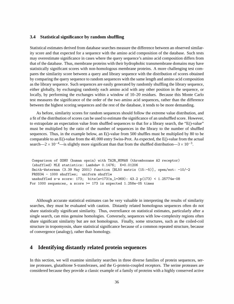
3.4 Statistical significance by random shuffling
Statistical estimates derived from database searches measure the difference between an observed similar-ity score and that expected for a sequence with the amino acid composition of the database. Such testsmay overestimate significance in cases where the query sequence’s amino acid composition differs fromthat of the database. Thus, membrane proteins with their hydrophobic transmembrane domains may havestatistically significant scores with non-homologous membrane proteins. A more challenging test com-pares the similarity score between a query and library sequence with the distribution of scores obtainedby comparing the query sequence to random sequences with the same length and amino acid compositionas the library sequence. Such sequences are easily generated by randomly shuffling the library sequence,either globally, by exchanging randomly each amino acid with any other position in the sequence, orlocally, by performing the exchanges within a window of 10–20 residues. Because this Monte Carlotest measures the significance of the order of the two amino acid sequences, rather than the differencebetween the highest scoring sequences and the rest of the database, it tends to be more demanding.
As before, similarity scores for random sequences should follow the extreme value distribution, anda fit of the distribution of scores can be used to estimate the significance of an unshuffled score. However,to extrapolate an expectation value from shuffled sequences to that for a library search, the “E()-value”must be multiplied by the ratio of the number of sequences in the library to the number of shuffledsequences. Thus, in the example below, an E()-value from 500 shuffles must be multiplied by 80 to becomparable to an E()-value from the 40,000 entry Swiss-Prot. As expected, the E()-value from the actualsearch—2×10⁻⁴—is slightly more significant than that from the shuffled distribution—3×10⁻³.
Comparison of OOHU (human opsin) with TA2R_HUMAN (thromboxane A2 receptor)(shuffled) MLE statistics: Lambda= 0.1476; K=0.01206Smith-Waterman (3.39 May 2001) function [BL50 matrix (15:-5)], open/ext: -10/-2PRSS34 - 1000 shuffles; uniform shuffleunshuffled s-w score: 173; bits(s=173|n_l=369): 43.2 p(173) < 1.25774e-08
For 1000 sequences, a score >= 173 is expected 1.258e-05 times
Although accurate statistical estimates can be very valuable in interpreting the results of similaritysearches, they must be evaluated with caution. Distantly related homologous sequences often do notshare statistically significant similarity. Thus, overreliance on statistical estimates, particularly after asingle search, can miss genuine homologies. Conversely, sequences with low-complexity regions oftenshare significant similarity but are not homologous. Finally, some structures, such as the coiled-coilstructure in tropomyosin, share statistical significance because of a common repeated structure, becauseof convergence (analogy), rather than homology.
4 Identifying distantly related protein sequences
In this section, we will examine similarity searches in three diverse families of protein sequences, ser-ine proteases, glutathione S-transferases, and the G-protein-coupled receptors. The serine proteases areconsidered because they provide a classic example of a family of proteins with a highly conserved active
36
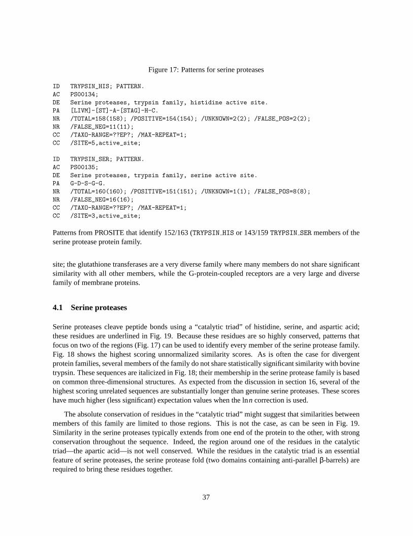
Figure 17: Patterns for serine proteases
ID TRYPSIN_HIS; PATTERN.AC PS00134;DE Serine proteases, trypsin family, histidine active site.PA [LIVM]-[ST]-A-[STAG]-H-C.NR /TOTAL=158(158); /POSITIVE=154(154); /UNKNOWN=2(2); /FALSE_POS=2(2);NR /FALSE_NEG=11(11);CC /TAXO-RANGE=??EP?; /MAX-REPEAT=1;CC /SITE=5,active_site;
ID TRYPSIN_SER; PATTERN.AC PS00135;DE Serine proteases, trypsin family, serine active site.PA G-D-S-G-G.NR /TOTAL=160(160); /POSITIVE=151(151); /UNKNOWN=1(1); /FALSE_POS=8(8);NR /FALSE_NEG=16(16);CC /TAXO-RANGE=??EP?; /MAX-REPEAT=1;CC /SITE=3,active_site;
Patterns from PROSITE that identify 152/163 (TRYPSIN HIS or 143/159TRYPSIN SER members of theserine protease protein family.
site; the glutathione transferases are a very diverse family where many members do not share significantsimilarity with all other members, while the G-protein-coupled receptors are a very large and diversefamily of membrane proteins.
4.1 Serine proteases
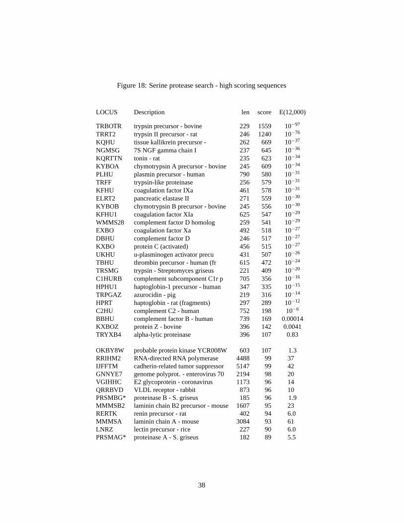
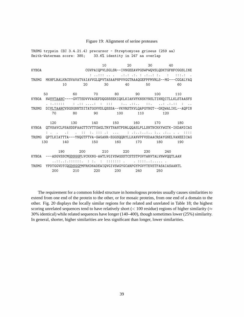
Serine proteases cleave peptide bonds using a “catalytic triad” of histidine, serine, and aspartic acid;these residues are underlined in Fig. 19. Because these residues are so highly conserved, patterns thatfocus on two of the regions (Fig. 17) can be used to identify every member of the serine protease family.Fig. 18 shows the highest scoring unnormalized similarity scores. As is often the case for divergentprotein families, several members of the family do not share statistically significant similarity with bovinetrypsin. These sequences are italicized in Fig. 18; their membership in the serine protease family is basedon common three-dimensional structures. As expected from the discussion in section 16, several of thehighest scoring unrelated sequences are substantially longer than genuine serine proteases. These scoreshave much higher (less significant) expectation values when the lnn correction is used.
The absolute conservation of residues in the “catalytic triad” might suggest that similarities betweenmembers of this family are limited to those regions. This is not the case, as can be seen in Fig. 19.Similarity in the serine proteases typically extends from one end of the protein to the other, with strongconservation throughout the sequence. Indeed, the region around one of the residues in the catalytictriad—the apartic acid—is not well conserved. While the residues in the catalytic triad is an essentialfeature of serine proteases, the serine protease fold (two domains containing anti-parallelβ-barrels) arerequired to bring these residues together.
37
Figure 18: Serine protease search - high scoring sequences
LOCUS Description len score E(12,000)
TRBOTR trypsin precursor - bovine 229 1559 10−97
TRRT2 trypsin II precursor - rat 246 1240 10−76
KQHU tissue kallikrein precursor - 262 669 10−37
NGMSG 7S NGF gamma chain I 237 645 10−36
KQRTTN tonin - rat 235 623 10−34
KYBOA chymotrypsin A precursor - bovine 245 609 10−34
PLHU plasmin precursor - human 790 580 10−31
TRFF trypsin-like proteinase 256 579 10−31
KFHU coagulation factor IXa 461 578 10−31
ELRT2 pancreatic elastase II 271 559 10−30
KYBOB chymotrypsin B precursor - bovine 245 556 10−30
The requirement for a common folded structure in homologous proteins usually causes similarities toextend from one end of the protein to the other, or for mosaic proteins, from one end of a domain to theother. Fig. 20 displays the locally similar regions for the related and unrelated in Table 18; the highestscoring unrelated sequences tend to have relatively short (< 100 residue) regions of higher similarity (≈30% identical) while related sequences have longer (140–400), though sometimes lower (25%) similarity.In general, shorter, higher similarities are less significant than longer, lower similarities.
All of the unitalicized sequences are known to be members of the glutathione transferase family.
41
4.2 Glutathione S-transferases
The glutathione transferase family of enzymes is a very diverse family of proteins found, in variousforms, in animals, plants, and prokaryotes. Fortunately, many of the members of this family have acommon enzyme activity so that they can be recognized by name. Table 14 shows that for this family,there are many homologues that do not show significant similarity when the database is searched with asingle query sequence.
Frequently, clear identification of a distant homology will require several database searches, witheither different algorithms or additional query sequences. For example, in Table 14, one might wishto test the possibility that glutathione S-transferases share homology with elongation factors, which areamong the high scoring sequences. The result of a search usingEF1G HUMAN is shown in Table 15. Here,there is a clear relationship between this elongation factor and the class-theta glutathione transferases.An additional search with a class-theta sequence reveals the most distant relationships in this family moreclearly.
The G-protein-coupled receptors (GCRs) are one of the largest known gene families; members of thefamily transduce signals from light, peptides, cationic amines, lipid mediators, odors, and many moresmall molecules. An evolutionary tree that summarizes the diversity of this family is shown in Fig. 21.Based on hydrophobicity plots and the structure of bacteriorhodopsin (a protein that does not share sig-nificant similarity with members of this family), the GCRs are thought to contain seven transmembranedomains, so that the N-terminus of the proteins is extracellular, while the C-terminus is intracellular.
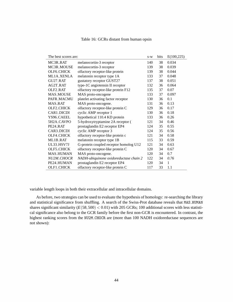
Because GCRs have transmembrane domains, the highest scoring unrelated sequences are frequentlyother membrane proteins. Table 16 lists sequences from Swiss-Prot that have marginally significantmatches with a human opsin sequence (there are more than 500 related sequences with expectationsranging from 0–0.01 that are not shown). As with most divergent families, the question becomes, “howdo I know that XXX is/is not a GCR?” This is more difficult with the GCRs, because they have long
43
Table 16: GCRs distant from human opsin
The best scores are: s-w bits E(100,225)
MC3R RAT melanocortin-3 receptor 140 38 0.034MC3R MOUSE melanocortin-3 receptor 139 38 0.039OLF6 CHICK olfactory receptor-like protein 139 38 0.044ML1A XENLA melatonin receptor type 1A 133 37 0.048GU27 RAT gustatory receptor GUST27 137 38 0.051AG2T RAT type-1C angiotensin II receptor 132 36 0.064OLF2 RAT olfactory receptor-like protein F12 135 37 0.07MAS MOUSE MAS proto-oncogene 133 37 0.097PAFR MACMU platelet activating factor receptor 130 36 0.1MAS RAT MAS proto-oncogene. 131 36 0.13OLF2 CHICK olfactory receptor-like protein C 129 36 0.17CAR1 DICDI cyclic AMP receptor 1 130 36 0.18YS96 CAEEL hypothetical 110.4 KD protein 133 36 0.265H2A CAVPO 5-hydroxytryptamine 2A receptor ( 121 34 0.46PE24RAT prostaglandin E2 receptor EP4 124 35 0.55CAR3 DICDI cyclic AMP receptor 3 124 35 0.56OLF4 CHICK olfactory receptor-like protein c 121 34 0.58ML1B RAT melatonin receptor type 1B 115 33 0.59UL33 HSV7J G-protein coupled receptor homolog U12 121 34 0.63OLF5 CHICK olfactory receptor-like protein C 120 34 0.67MAS HUMAN MAS proto-oncogene. 120 34 0.7NU2M CHOCR NADH-ubiquinone oxidoreductase chain 2122 34 0.76PE24HUMAN prostaglandin E2 receptor EP4 120 34 1OLF1 CHICK olfactory receptor-like protein C 117 33 1.1
variable length loops in both their extracellular and intracellular domains.
As before, two strategies can be used to evaluate the hypothesis of homology: re-searching the libraryand statistical significance from shuffling. A search of the Swiss-Prot database reveals thatMAS HUMANshares significant similarity (E(58,500)< 0.01) with 205 GCRs; 100 additional scores with less statisti-cal significance also belong to the GCR family before the first non-GCR is encountered. In contrast, thehighest ranking scores from theNU2M CHOCR are (more than 100 NADH oxidoreductase sequences arenot shown):
The results from theMAS HUMAN andNU2M CHOCR, which show thatMAS HUMAN is clearly a memberof the GCR family, contrast with the statistical significance calculated with thePRSS program. Com-paring theOOHU with RTA RAT score with the distribution of scores calculated after shufflingRTA RAT1000 times with a local window of 20 suggests that the unshuffled score (109 ) is expected 6 times in1000 shuffles. In contrast, theNU2M CHOCR score is expected only 1.7 times in 1000 shuffles. From thisperspective, theNU2M CHOCR score is somewhat more significant, but, in fact, neither similarity score isstatistically significant. It is not untilMAS HUMAN is compared with other members of the family, e.g. theangiotensin, fMet-Leu-Phe, thrombin, or substance-P receptors with E-values from 10−12–10−6, that therelationship is apparent.
Table 3.3 compares the statistical significance inferred from database searches with those determinedby Monte-Carlo shuffling. As expected, the significance of the scores when compared with locally (win-dow) shuffled sequences is 10-fold lower than the comparison with globally shuffled scores. It is unclearhow to compare the expectation from shuffles with the expectation from a search. In the table, the ex-pectation from a search of a 43,000 entry library is compared to the expectation from 1,000 shuffles.For global shuffles, the expectations are quite comparable while local shuffles are more conservative, yetall but one of the similarity scores judged significant from the database search are still significant whencompared with the local-shuffle distribution.
Nevertheless, these examples show both that current statistical models for the similarity scores ofunrelated sequences are quite accurate, but also that homologous sequences frequently do not sharesignificant pair-wise similarity scores. Thus, a lack of statistical significance cannot be used to infernon-homology, but strong statistical significance is a good indicator of common ancestry.
45
Figure 22: Internal duplications in calmodulin
10 140
CALM_HUMAN calmodulin - human
10
140
A B C D
AB
CD
CA
LM
_H
UM
AN
ca
lmo
du
lin -
hu
ma
n
33/1
02; E
()<10-4
31/6
5; E()<
10-6
148/
148;
E()=0
13/3
6; E()>
10
Comparison of human calmodulin with itself. Each diagonal line represents a potential local alignmentof calmodulin with itself. Values below the diagonal lines show the number of identities and length ofthe aligned region (e.g. 33/102) and the expectation value for the similarity score of the alignment.
5 Repeated structures in proteins
So far, we have focussed on the identification and statistics of the single most significant similarityscore shared by two sequences. As can be seen in Fig. 10B, however, there are frequently several non-overlapping local alignments with optimal similarity scores. In addition, there can be non-overlappingsub-optimal alignments with significant scores that can be used to infer the duplication events that gaverise to the protein sequence. An algorithm for the bestN non-overlapping local alignments was describedby (Waterman & Eggert, 1987).
Figs. 22 and 23 show a graphical plot of the local similarities within the calmodulin calcium bindingprotein. Calmodulin contains four EF-hand Ca+-binding domains that are well conserved. The highestscoring alignment in Fig. 23 aligns domainsA-B with C-D; the second highest alignsA-B-C with B-C-D;the third alignsA with D.
A similar pattern of local similarity can be seen in Fig. 24, which shows the mosaic relationshipbetween the EGF-precursor and the LDL-receptor.
46
Figure 23: Calmodulin internal alignments
Comparison of:(A) MCHU - Calmodulin - Human, rabbit, bovine, rat, - 148 aa(B) MCHU - Calmodulin - Human, rabbit, bovine, rat, - 148 aausing matrix file: BLOSUM50, gap penalties: -14/-4
47.7% identity in 65 aa overlap; score: 214 E(10,000): 3.4e-13
Some non-homologous structures, particularly proteins containing the coiled-coil structure, havea periodic structure that is easily seen in local similarity plots. Fig. 25 shows local similarities intropomyosin. All the alignments shown have local similarity scores greater than 120, and each would besignificant in a conventional database search.
6 Summary
Protein sequence comparison is the most powerful tool available today for inferring structure and functionfrom sequence because of the constraints of protein evolution—a protein fold into a functional structure.Protein sequence similarity can routinely be used to infer relationships between proteins that last shared acommon ancestor 1–2.5 billion years ago. Our ability to identify distantly related proteins has improvedover the past five years with the development of accurate statistical estimates, which have provided betternormalization methods, and with the use of optimized scoring parameters. In using sequence similarityto infer homology, one should remember:
1. Always compare protein sequences if the genes encode proteins. Protein sequence comparisonwill typically double the look back time over DNA sequence comparison.
2. While most sequences that share statistically significant similarity are homologous, many distantlyrelated homologous sequences do not share significant homology. (Low complexity regions can
48
Figure 25: Coiled-coil structures share local similarity
20 280TMRBA tropomyosin alpha chain, cardiac
20
280
TMRBA tropomyosin alpha chain, cardiac
<0.0001<0.01
<1<1e+02
>1e+02
display significant similarity in the absence of homology). Homologous sequences are usuallysimilar over an entire sequence or domain. Matches that are more than 50% identical in a 20–40amino acid region occur frequently by chance.
3. Homologous sequences share a common ancestor, and thus a common protein fold. Dependingon the evolutionary distance and divergence path, two or more homologous sequences may havevery few absolutely conserved residues. However, if homology has been inferred betweenA andB, betweenB andC, and betweenC andD, A andD must be homologous, even if they share nosignificant similarity.
4. Similarity searching techniques can be improved either by increasing the ability of a method torecognize distantly related sequences—increased sensitivity—or by lowering scores for unrelatedsequences—increased selectivity. Since there are generally 1000-times more unrelated than relatedsequences in a sequence database, improvements that reduce the scores of unrelated sequences canhave dramatic effects. The most dramatic improvements in comparison methods recently haveused this approach.
49
References
Altschul, S. F. (1991). Amino acid substitution matrices from an information theoretic perspective.J.Mol. Biol. 219, 555–565.
Altschul, S. F. (1993). A protein alignment scoring system sensitive at all evolutionary distances.J. Mol.Evol.36, 290–300.
Altschul, S. F., Boguski, M. S., Gish, W. & Wootton, J. C. (1994). Issues in searching molecular sequencedatabases.Nature Genet.6, 119–129.
Altschul, S. F., Gish, W., Miller, W., Myers, E. W. & Lipman, D. J. (1990). Basic local alignment searchtool. J. Mol. Biol.215, 403–410.
Collins, J. F., Coulson, A. F. W. & Lyall, A. (1988). The significance of protein sequence similarities.Comp. Appl. Biosci.4, 67–71.
Dayhoff, M., Schwartz, R. M. & Orcutt, B. C. (1978). A model of evolutionary change in proteins. InAtlas of Protein Sequence and Structure, (Dayhoff, M., ed.), vol. 5, supplement 3, pp. 345–352.National Biomedical Research Foundation Silver Spring, MD.
Doolittle, R. F., Feng, D. F., Johnson, M. S. & McClure, M. A. (1986). Relationships of human proteinsequences to those of other organisms.Cold Spring Harb. Symp. Quant. Biol.51, 447–455.
Gilbert, W. & Glynias, M. (1993). On the ancient nature of introns.Gene,135, 137–144.
Henikoff, S. & Henikoff, J. G. (1992). Amino acid substitutions matrices from protein blocks.Proc.Natl. Acad. Sci. USA,89, 10915–10919.
Henikoff, S. & Henikoff, J. G. (1993). Performance evalutation of amino-acid substitution matrices.Proteins, 17, 49–61.
Johnson, M. S. & Overington, J. P. (1993). A structural basis for sequence comparisons. an evaluation ofscoring methodologies.J. Mol. Biol.233, 716–738.
Jones, D. T., Taylor, W. R. & Thornton, J. M. (1992). The rapid generation of mutation data matricesfrom protein sequences.Comp. Appl. Biosci.8, 275–282.
Karlin, S. & Altschul, S. F. (1990). Methods for assessing the statistical significance of molecular se-quence features by using general scoring schemes.Proc. Natl. Acad. Sci. USA,87, 2264–2268.
Karlin, S. & Altschul, S. F. (1993). Applications and statistics for multiple high-scoring segments inmolecular sequences.Proc. Natl. Acad. Sci. U S A,90, 5873–7.
Mott, R. (1992). Maximum-likelihood estimation of the statistical distribution of smith-waterman localsequence similarity scores.Bull. Math. Biol.54, 59–75.
Needleman, S. & Wunsch, C. (1970). A general method applicable to the search for similarities in theamino acid sequences of two proteins.J. Mol. Biol.48, 444–453.
Nei, M. (1987).Molecular Evolutionary Genetics. Columbia Univ. Press, New York, NY.
50
Pearson, W. R. (1995). Comparison of methods for searching protein sequence databases.Prot. Sci.4,1145–1160.
Pearson, W. R. (1998). Empirical statistical estimates for sequence similarity searches.J. Mol. Biol.276,71–84.
Pearson, W. R. & Lipman, D. J. (1988). Improved tools for biological sequence comparison.Proc. Natl.Acad. Sci. USA,85, 2444–2448.
Smith, T. F. & Waterman, M. S. (1981). Identification of common molecular subsequences.J. Mol. Biol.147, 195–197.
Stoltzfus, A., Spencer, D. F., Zuker, M., Logsdon, J. M. & Doolittle, W. F. (1994). Testing the introntheory of genes: the evidence from protein structure.Science,265, 202–207.
Waterman, M. S. & Eggert, M. (1987). A new algorithm for best subsequences alignment with applicationto tRNA-rRNA comparisons.J. Mol. Biol.197, 723–728.
51
7 Suggested Reading
7.1 General Protein evolution
R. F. Doolittle, D. F. Feng, M. S. Johnson, and M. A. McClure. Relationships of human protein sequencesto those of other organisms.Cold Spring Harb. Symp. Quant. Biol., 51:447–455, 1986.
R. F. Doolittle The multiplicity of domains in proteinsAnnu. Rev. Biochem., 64:287–314, 1995.
7.1.1 Introns Early/Late
W. Gilbert and M. Glynias. On the ancient nature of introns.Gene, 135:137–144, 1993.
A. Stoltzfus, D. F. Spencer, M. Zuker, J. M. Logsdon, and W. F. Doolittle. Testing the intron theory ofgenes: the evidence from protein structure.Science, 265:202–207, 1994.
7.2 Alignment methods
7.2.1 Algorithms
S. Needleman and C. Wunsch. A general method applicable to the search for similarities in the aminoacid sequences of two proteins.J. Mol. Biol., 48:444–453, 1970.
T. F. Smith and M. S. Waterman. Identification of common molecular subsequences.J. Mol. Biol.,147:195–197, 1981.
W. R. Pearson and W. Miller. Dynamic programming algorithms for biological sequence comparison.In L. Brand and M. L. Johnson, editors,Meth. Enz., volume 210, pages 575–601. Academic Press, SanDiego, 1992.
D. J. Lipman and W. R. Pearson. Rapid and sensitive protein similarity searches.Science, 227:1435–1441, 1985.
W. R. Pearson and D. J. Lipman. Improved tools for biological sequence comparison.Proc. Natl. Acad.Sci. USA, 85:2444–2448, 1988.
W. R. Pearson. Rapid and sensitive sequence comparison with FASTP and FASTA. In R. F. Doolittle,editor,Meth. Enz., volume 183, pages 63–98. Academic Press, San Diego, 1990.
S. F. Altschul, W. Gish, W. Miller, E. W. Myers, and D. J. Lipman. A basic local alignment search tool.J. Mol. Biol., 215:403–410, 1990.
S. F. Altschul, T. L. Madden, A. A. Schaffer, J. Zhang, Z. Zhang, W. Miller, and D. J. Lipman. GappedBLAST and PSI-BLAST: a new generation of protein database search programsNucleic Acids Res.,25:3389–3402, 1997.
W. R. Pearson. Empirical statistical estimates for sequence similarity searchesJ. Mol. Biol. 276:71–84,1998.
52
7.2.2 Scoring methods
M. Dayhoff, R. M. Schwartz, and B. C. Orcutt. A model of evolutionary change in proteins. In M. Day-hoff, editor,Atlas of Protein Sequence and Structure, volume 5, supplement 3, pages 345–352. NationalBiomedical Research Foundation, Silver Spring, MD, 1978.
S. F. Altschul. Amino acid substitution matrices from an information theoretic perspective.J. Mol. Biol.,219:555–565, 1991.
D. T. Jones, W. R. Taylor, and J. M. Thornton. The rapid generation of mutation data matrices fromprotein sequences.Comp. Appl. Biosci., 8:275–282, 1992.
S. Henikoff and J. G. Henikoff. Performance evalutation of amino-acid substitution matrices.Proteins,17:49–61, 1993.
7.3 Evaluating matches - statistics of similarity scores
S. F. Altschul, M. S. Boguski, W. Gish, and J. C. Wootton. Issues in searching molecular sequencedatabases.Nature Genet., 6:119–129, 1994.
S. F. Altschul, and W. Gish. Local Alignment StatisticsMeth. Enzymol., 266:460–480, 1996.