A Proposal to Measure the Proton

Electric Dipole Moment with 10-29ecm

Sensitivity

by the Storage Ring EDM Collaboration

October 2011

ii

Storage Ring EDM Collaboration V. Anastassopoulos18, D. Babusci10, M. Bai3, S. Baessler23, M. Berz17, M. Blaskiewicz3,

K. Brown3, P. Cameron3, G. Daskalakis6, N. D’ Imperio3, M.E. Emirhan13, F. Esser24,

G. Fanourakis6, A. Fedotov3, A. Ferrari25, W. Fischer3, T. Geralis6, Y. Giomataris21,

F. Gonnella20, M. Gross Perdekamp11, R. Gupta3, G. Guidoboni8, S. Haciomeroglu13,3,

Y. Haritantis18, G. Hoffstaetter5, H. Huang3, M. Incagli19, D. Kawall16, B. Khazin4,

I.B. Khriplovich4, I.A. Koop4, T. Laopoulos1, R. Larsen3, D.M. Lazarus3, A. Lehrach9,

P. Lenisa8, P. Levi Sandri10, F. Lin3, A.U. Luccio3, A. Lyapin15, W.W. MacKay3,

R. Maier9, K. Makino17, N. Malitsky3, W. Marciano3, S. Martin26, W. Meng3, F. Meot3,

R. Messi20, D. Moricciani20, W.M. Morse3, S.K. Nayak3, Y.F. Orlov5, C.S. Ozben13,

A. Pesce8, V. Ptitsyn3, B. Parker3, P. Pile3, V. Polychronakos3, B. Podobedov3,

D. Raparia3, F. Rathmann9, S. Redin4, S. Rescia3, G. Ruoso14, T. Russo3, N. Saito22,

J. Seele28, Y.K. Semertzidis3,*, Yu. Shatunov4, V. Shemelin5, A. Sidorin7, A. Silenko2,

N. Simos3, S. Siskos1, A. Stahl27, E.J. Stephenson12, H. Stroeher9, J. Talman3,

R.M. Talman5, P. Thieberger3, N. Tsoupas3, Y. Valdau9, G. Venanzoni10, K. Vetter3,

S. Vlassis18, G. Zavattini8, A. Zelenski3, K. Zioutas18

1Electronics Lab., Physics Dept., Aristotle University of Thessaloniki, GR-54124

Thessaloniki, Greece 2Research Inst. for Nucl. Probl. of Belarusian State University, Minsk, Belarus

3Brookhaven National Laboratory, Upton, NY 11973, USA 4Budker Institute of Nuclear Physics, 630090 Novosibirsk, Russia

5Laboratory for Elementary-Particle Physics, Cornell University, Ithaca, NY 14853, USA 6Inst. of Nuclear Physics NCSR Demokritos, GR-15310 Aghia Paraskevi Athens, Greece

7Joint Institute for Nuclear Research, Dubna, Moscow region, Russia 8University of Ferrara, INFN of Ferrara, Ferrara, Italy

9Institut für Kernphysik, Forschungszentrum Jülich, 52425 Jülich, Germany 10Laboratori Nazionali di Frascati, INFN, I-00044 Frascati, Rome, Italy

iii

11Dept. of Physics, Univ. of Illinois at Urbana-Champaign, IL 61801, USA 12Center for Exploration of Energy and Matter, Indiana University, Bloomington, IN

47408, USA 13Istanbul Technical University, Istanbul 34469, Turkey

14Legnaro National Laboratories of INFN, Legnaro, Italy 15Royal Holloway, University of London, Egham, Surrey, UK

16Dept. of Physics, University of Massachusetts, Amherst, MA 01003, USA 17Dept. of Physics and Astron., Michigan State University, East Lansing, MI 48824, USA

18Department of Physics, University of Patras, 26500 Rio-Patras, Greece 19Physics Department, University and INFN Pisa, Italy

20Dipartimento di Fisica dell’Università di Roma “Tor Vergata”

and INFN Sezione di Roma Tor Vergata, Roma, Italy 21CEA/Saclay, DAPNIA, 91191 Gif-sur-Yvette Cedex, France

22KEK, High Energy Accel. Research Organization, Tsukuba, Ibaraki 305-0801, Japan 23Dept. of Physics, University of Virginia, Charlottesville, VA 22904, USA

24ZAT Central Technology Division, Forschungszentrum Jülich, 52425 Jülich, Germany 25Helmholtz-Zentrum Dresden-Rossendorf (HZDR), Germany

26UGS Gerlinde Schulteis & Partner, Hauptstrasse 75, 08428 Langenbernsdorf, Germany 27RWTH Aachen, Physikalisches Institut, Physikzentrum, 52056 Aachen, Germany

28RIKEN BNL Research Center, BNL, Upton, NY 11973, USA

*Spokesperson: Yannis K. Semertzidis (yannis@bnl.gov, 631-344-3881)

iv

Contents

Abstract vii

1. Introduction 1

2. Motivation for Proton and Deuteron EDM Measurements 7

2.1 The QCD CP-Violating Parameter 8

2.2 Supersymmetry 9

2.3 Dimensional analysis 10

3. Experimental Method 11

3.1 The all-electric field ring 12

3.2 Basic all-electric field beam dynamics 13

3.3 Basic measurement sequence 14

3.4 Basic experiment performance requirements 15

4. Ring Lattice for the Experiment 19

4.1 Requirements imposed by the experiment 19

4.2 Implications of electric (rather than magnetic) bending 20

4.3 Lattice design considerations 22

4.4 Transverse dynamics 23

4.5 Injection 25

5. Beam Parameters at BNL 27

6. Beam and Spin Tracking Simulations 29

6.1 SCT simulation studies using the 4th-order Runge-Kutta integration method 30

6.2 Simulation studies of the effect of straight section length on SCT 31

7. Spin Coherence Time Experiment 35

7.1 Overview 35

7.2 Preliminary results from the January 2011 run 36

8. Electric and Magnetic Fields 37

8.1 Spin preparation solenoid 37

8.2 Electric field overview 37

8.3 Choice of electrode material 37

8.4 System design 41

8.5 New methods for higher DC HV 42

v

8.6 Sparks during the pEDM run 44

8.7 Patch effect 45

8.8 Magnetic fields 45

8.9 Electric field R&D: constructing the first E module 47

9. Relative Beam Position Monitors 50

9.1 Measuring Bro 50

9.2 Sensitive magnetometry using SQUIDS 50

9.3 Earth’s magnetic field shielding 52

9.4 Time dependent magnetic field shielding 53

10. Polarimeter 55

10.1 Overview 55

10.2 Polarimeter design 55

10.3 A possible EDM polarimeter 56

10.4 Suppression of geometric and rate errors in real time 57

10.5 Operating characteristics of the polarimeter test at COSY 60

10.6 Future plans 61

11. Statistical Sensitivity and Systematic Errors of the Experimental Method 62

11.1 Expected signal of the pEDM experiment 62

11.2 Statistical error 62

11.3 Systematic errors of the pEDM experiment 66

12. R&D: Experimental Issues, Costs, Timeline, and Goals 75

12.1 Main experimental issues 75

12.2 Estimated costs 76

12.3 R&D timeline 76

12.4 Comments about R&D plans 78

13. Cost of the Experiment 79

Acknowledgements 83

vi

Appendices

Appendix 1. R. Talman, Ring Lattice for Proton EDM Measurement, July 2011. Appendix 2. N. Malitsky, J. Talman, and R. Talman, Development of the UAL/ETEAPOT Code for the Proton EDM Experiment, June 2011. Appendix 3. R. Talman, Parameters of Proton EDM Trial Lattices, April 2011. Appendix 4. S. Haciomeroglu and Y.K. Semertzidis, SCT with 4th-Order Runge-Kutta Simulations, June 2011. Appendix 5. W. Morse, Electric and Magnetic Fields, February 2011. Appendix 6. D. Kawall, Relative Beam Position Monitors for the pEDM Experiment, June 2011. Appendix 7. E.J. Stephenson et al., Polarimeter appendix: Correcting Systematic Errors in High Sensitivity Deuteron Polarization Measurements, June 2011. Appendix 8. K. Vetter, NSLS-II RF Button BPM, June 2011. Appendix 9. M. Berz and K. Makino, Advanced Computational Methods for Nonlinear Spin Dynamics, September 2010.

vii

ABSTRACT

The storage ring EDM collaboration proposes a new method to search for and measure the electric dipole moment of the proton by using polarized protons at the so-called “magic” momentum of 0.7 GeV/c in an all-electric storage ring with radius of ~40 m and an E-field of ~10 MV/m between plates separated by 3 cm. The sensitivity level (10-29 ecm) will be one or two orders of magnitude greater than that of hadronic EDM experiments being planned elsewhere. The strength of the storage ring EDM method comes from the fact that we can store a large number of highly polarized particles for a long time, achieve a large horizontal spin coherence time (SCT), and probe the transverse spin components as a function of time with a high sensitivity polarimeter.

At their magic momentum of 0.7 GeV/c, the proton spin and momentum vectors precess at the same rate in any transverse electric field. When the spin is kept along the momentum direction, the radial electric field acts on the EDM vector and precesses the proton spin vertically for the duration of the storage time, building up its vertical component. The storage time is limited to 103 s by the estimated SCT of the beam within the admittance of the ring. Stochastic cooling might be used to extend the SCT and experimental sensitivity by another order of magnitude. Having considered various methods of “freezing” the spin along the momentum direction by applying a combination of magnetic and electric fields, the collaboration believes that the proton EDM method at the magic momentum using only electric fields is the simplest to implement.

For contact interactions, the mass scale sensitivity is at the 3000 TeV range, and for SUSY-like new physics 300 TeV. If there is new physics at the LHC scale, the experiment will be able to probe CP-violating phases down to 0.1 rad, making it the most sensitive probe for CP-violation beyond the standard model. Moreover, it can test the electro-weak baryogenesis models of the mechanism responsible for the observed baryon asymmetry in our universe.

The method is patterned after the celebrated muon g-2 experiment, on which about half the collaboration has previously worked. The collaboration has had two successful technical reviews by experts in the field: one in December 2009 and one in March 2011. Running with polarized deuteron beams at KVI (Groningen/The Netherlands) and beams stored in COSY (Jülich/Germany), we have shown the polarimeter systematic errors to be well below our statistical sensitivity level.

The collaboration's understanding of and confidence in the proposed experimental method are the result of many years of development, during which we have studied polarimeter systematic errors, efficiency and analyzing power; developed a tracking program that can accurately simulate the spin and beam dynamics of stored particles in an all-electric ring; developed E-field measurements at BNL, using technology developed as part of the international linear collider (ILC) and energy recovery linacs (ERL) R&D efforts; developed a plan to build a beam position monitor system capable of probing the main systematic error source in the experiment (an average radial B-field around the

viii

ring); and established that using commonly achievable position tolerances and beam- based alignment in the relative positioning of E-field plates around the ring will reduce geometrical phase effects to a level well below the EDM signal.

Thus, the collaboration believes it is securely positioned to request, with this proposal, a CD0 to develop a proton EDM experiment with sensitivity of 10-29 ecm, as well as $2M to conclude our R&D effort.

1

1. INTRODUCTION General context. In quantum mechanics, a non-degenerate system with spin is defined by the spin vector. If a particle has an electric dipole moment (EDM), the vector of the EDM is aligned with the spin vector of the particle. The EDM then violates both time (T) and parity (P) symmetries and conserves charge (C) symmetry. Assuming conservation of the combined CPT symmetry, T-violation also means CP-violation. The weak interaction CP-violation contributes a very small EDM, one that is orders of magnitude below current experimental limits. However, most models beyond the standard model (SM) predict EDM values near the current experimental limits. Hence, the study of EDMs is a search for CP-violation beyond the SM. Finding a non-zero EDM value will point to a new, strong CP-violating source, which is needed to solve the mystery of the baryon-antibaryon asymmetry of our universe.

We plan to search for the EDM of the proton in a storage ring with a statistical sensitivity of 1.3×10-29 ecm per year. This level of sensitivity will be an order of magnitude greater than that of the currently planned neutron EDM experiments at SNS (Oak Ridge, Tennessee), PSI (Villigen, Switzerland), and ILL (Grenoble, France). After a major upgrade, the ring could accommodate a deuteron EDM experiment with similar sensitivity. Technical requirements. We plan to measure the proton EDM by observing the spin precession in an external electric field. This approach has limited previous experiments to neutral systems (neutrons, atoms) to avoid accelerating the trapped particles. However, the storage ring can use this electric field to confine the particles to a closed path, thus opening up the domain of EDM experiments to charged particles, ions, and other species.

The stored beam must be spin polarized. Given that the best sensitivity may involve rotations as small as micro-radians, it is prudent to begin with the spins aligned parallel to the beam momentum; then the radial electric field acting on an EDM will precess these spins into the vertical direction (out of the ring plane), where the growing polarization component is stable and measurable. This imposes two requirements: the storage ring lattice must be capable of (1) defeating the tendency of the spins to precess in the ring plane so that they remain longitudinal, and (2) maintaining the spin coherence for times long enough to accumulate a measurable EDM precession. For the proton or any charged particle with a positive anomalous magnetic moment, the first requirement is met by operating the storage ring at the so-called “magic” momentum (p = 0.7 GeV/c for the proton), where the precession induced in the proton frame by v × E is just enough to match the rotation of the velocity vector (v). The second requirement makes it necessary to limit those properties of a stored beam, including momentum spread and emittance, that alter the v × E precession rate enough to cause the spin directions in the beam to disperse. These considerations led to the ring design described in Section 4. A development project is already underway at the COSY ring at the Forschungszentrum-Jülich (see Section 7) to demonstrate that such control is possible through a combination

2

of beam cooling techniques and the proper setting of higher-order fields (e.g., sextupole and beyond).

For the ring to be of a practical size, large electric fields are needed, up to 10.5 MV/m. Current technologies in use at laboratories such as Fermilab, and improved at Jefferson Lab and Cornell, have achieved larger electric fields with a combination of careful surface preparation, including electro-polishing and high pressure water rinsing (see Section 8). External magnetic fields that would perturb the spin precession must be measured to an accuracy of 1 nG at 1 Hz in the radial direction averaged around the ring. This requires a multilayer shield (both active and passive) as well as a way to monitor the success of the field suppression. Consideration of this problem led to the idea that a crucial way to control systematic errors would be doing the experiment with two beams traveling around the storage ring along the same path but in opposite directions. These two beams, which are dispersed enough to minimize any significant effects from inter-beam scattering, in fact represent the time reverse of each other. An EDM, being T-violating, responds oppositely to a large class of systematic errors that are T-conserving. The radial magnetic field is the main source of systematic errors, since it produces a vertical spin rotation signal just like an EDM. In addition, the radial magnetic field causes the two counter-rotating beams to separate vertically inside the ring, a fact that can be observed using suitable beam position monitoring equipment down to a level small enough to meet the sensitivity goal of this experiment (see Section 9).

Lastly, the experiment must provide a technique for measuring the several micro-radians change in the average spin direction between the beginning and the end of the beam store. At the magic momentum of the stored protons, we happen to be almost on top of the peak in spin sensitivity for protons elastically scattered from carbon nuclei. The storage ring plan includes a mechanism for slowly extracting particles from the beam to a point where they enter a carbon target block several centimeters thick. This thickness is enough to raise to nearly 1% the efficiency of spin-dependent scattering into a detector array that surrounds the beam, with counting changes due to a flip of the spin direction that exceed 60%. Experiments at COSY have already demonstrated that systematic errors from counting rate and geometric changes can be managed to well below one part per million, by using counting rates available from beam bunches with opposite spin orientations and a suitable calibration (see Section 10).*

The Brookhaven National Laboratory has sufficient accelerator assets already in place, as well as available space to site a new machine for the proposed proton EDM measurement. We would use the existing polarized proton beam and the Booster-Accumulator, and would feed the beam through the Alternating Gradient Synchrotron (AGS) to the EDM ring site.

* Other sections of this proposal give an overview of the scientific justification and important experimental considerations of the proposed project: motivation of the experiment (Section 2), the experimental method (Section 3), the ideal beam parameters (Section 5), beam and spin dynamics simulations (Section 6), the statistical limits of the experiment and the management of systematic errors (Section 11), the R&D goals and timeline (Section 12), and budget (Section 13). A set of Appendices gives details of the extensive work that has been done or is underway to demonstrate the feasibility of the experiment.

3

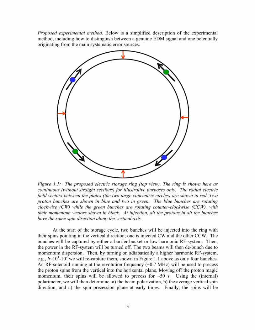
Proposed experimental method. Below is a simplified description of the experimental method, including how to distinguish between a genuine EDM signal and one potentially originating from the main systematic error sources.

Figure 1.1: The proposed electric storage ring (top view). The ring is shown here as continuous (without straight sections) for illustrative purposes only. The radial electric field vectors between the plates (the two large concentric circles) are shown in red. Two proton bunches are shown in blue and two in green. The blue bunches are rotating clockwise (CW) while the green bunches are rotating counter-clockwise (CCW), with their momentum vectors shown in black. At injection, all the protons in all the bunches have the same spin direction along the vertical axis.

At the start of the storage cycle, two bunches will be injected into the ring with their spins pointing in the vertical direction; one is injected CW and the other CCW. The bunches will be captured by either a barrier bucket or low harmonic RF-system. Then, the power in the RF-system will be turned off. The two beams will then de-bunch due to momentum dispersion. Then, by turning on adiabatically a higher harmonic RF-system, e.g., h~101-102 we will re-capture them, shown in Figure 1.1 above as only four bunches. An RF-solenoid running at the revolution frequency (~0.7 MHz) will be used to precess the proton spins from the vertical into the horizontal plane. Moving off the proton magic momentum, their spins will be allowed to precess for ~50 s. Using the (internal) polarimeter, we will then determine: a) the beam polarization, b) the average vertical spin direction, and c) the spin precession plane at early times. Finally, the spins will be

4

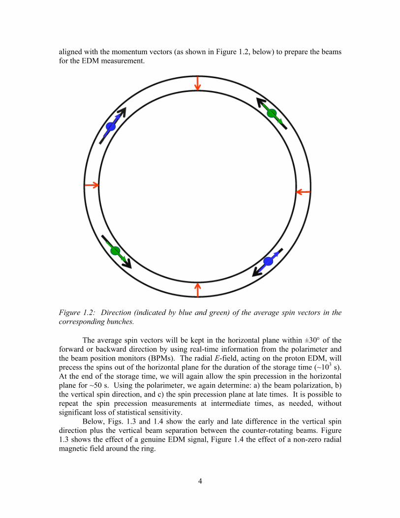
aligned with the momentum vectors (as shown in Figure 1.2, below) to prepare the beams for the EDM measurement.

Figure 1.2: Direction (indicated by blue and green) of the average spin vectors in the corresponding bunches.

The average spin vectors will be kept in the horizontal plane within ±30 of the forward or backward direction by using real-time information from the polarimeter and the beam position monitors (BPMs). The radial E-field, acting on the proton EDM, will precess the spins out of the horizontal plane for the duration of the storage time (~103 s). At the end of the storage time, we will again allow the spin precession in the horizontal plane for ~50 s. Using the polarimeter, we again determine: a) the beam polarization, b) the vertical spin direction, and c) the spin precession plane at late times. It is possible to repeat the spin precession measurements at intermediate times, as needed, without significant loss of statistical sensitivity. Below, Figs. 1.3 and 1.4 show the early and late difference in the vertical spin direction plus the vertical beam separation between the counter-rotating beams. Figure 1.3 shows the effect of a genuine EDM signal, Figure 1.4 the effect of a non-zero radial magnetic field around the ring.

5

Figure 1.3: A side view of the spin direction in the various bunches at early (a) and late (b) times, assuming a proton EDM is present. The storage ring has been unfolded into an imaginary straight line. The blue bunches travel to the right while the green bunches travel to the left. The EDM signal is the difference of the average vertical spin component between early and late times. The difference between the spin precession rates of the blue bunches with opposite spin directions is needed to reduce the polarimeter systematic errors to well below our anticipated sensitivity level (see Section 10). Comparisons with the corresponding difference in the green bunches eliminates systematic errors due to, e.g., vertical image charges (see Section 11, Table 11.1 of systematic errors).

Figure 1.4: A side view of the spin direction and vertical positions of the various bunches at early (a) and late (b) times, assuming the presence of a constant radial B-field--the main systematic error source in the experiment. Obviously, the vertical spin precession signal is very similar to that from a proton EDM. The difference is that the counter-rotating bunches move vertically in opposite directions, depending on the strength of the vertical focusing. The vertical tune will be low (~0.1) to enhance the beam separation and will be modulated with an amplitude of ~10% of itself, i.e., ~0.01 at a frequency of our choice in the range of 10 Hz – 10 KHz. The counter-rotating beams will oscillate vertically with the same frequency and amplitude of 1pm for a 10-29ecm sensitivity level (See Section 9).

6

Technical reviews. The collaboration has had two very successful technical reviews on the storage ring EDM method: one in December 2009 http://www.bnl.gov/edm/review/ and one in March 2011. The December 2009 review focused on the magic proton momentum, with CW and CCW rotating beams and momentum bending provided by electric field elements. At that time, the collaboration was working on two focusing options, one magnetic and the other electric. The review committee strongly recommended using an all-electric ring (including electric focusing), simplifying the experiment in several ways. Assuming a complete absence of magnetic fields, the CW and CCW beams will have exactly the same beta-functions everywhere in the ring and the beams will go through exactly the same positions. Most precisely, their closed orbits will be the same.

In addition, effects like geometrical phases (see Section 11), which are very important for the neutron EDM experiments, are much easier to guard against. We plan to eliminate magnetic fields to well below the requirements imposed by the geometrical phase effect, by using the BPM information in both the horizontal and vertical directions. The electric field by itself cannot cause a first-order problem because the magic-momentum proton spins do not precess in any electric field. However, geometric phase effects could result from electric field plate misalignment and placement errors. The construction requirements to produce a geometrical phase effect below our sensitivity level are well within the current state of the art and are easily (and cheaply) achievable. In addition, we are studying the possibility of using more than one azimuthal location around the ring as a polarimeter section, making visible the two possible lowest-order geometrical effects, which are most likely to dominate.

To increase the position splitting of the counter-rotating beams due to spurious magnetic fields, weak vertical and horizontal focusing will be used. This will have the additional benefit of substantially increasing the horizontal spin coherence time (SCT), thus further simplifying the experiment.

In the second review (March 2011), the all-electric ring method--including the sensitive BPM magnetometer system--was presented. The committee was enthusiastic about the method and encouraged the collaboration to proceed with the proposal.

With this proposal we request a Critical Decision 0 (CD0) for a storage ring proton EDM experiment with a sensitivity of 10-29ecm. Some R&D funding is needed now to establish the viability of the beam position monitors with the required sensitivity in an accelerator environment. It is also needed to finalize the E-field strength that we can safely apply between large area stainless steel plates, which will determine the storage ring radius. Finally, it will allow us to continue the spin coherence time studies at COSY that are needed to benchmark our tracking simulations software, as well as develop a polarimeter prototype to be commissioned at COSY. The above R&D support is essential for a future smooth transition from CD0 into CD1-3. Its total cost is estimated to be $2M, with a duration of approximately 2 years of a technically-driven schedule, as outlined in Section 12.

7

2. MOTIVATION FOR PROTON AND DEUTERON EDM MEASUREMENTS

Modern interest in elementary particle and bound-state electric dipole moments (EDMs) stems from the pioneering work of Norman Ramsey and his collaborators [1]. Their more than 50-year quest to find a neutron EDM anticipated parity (P) and time-reversal (T or CP) violation, necessary ingredients for the existence of a non-zero EDM. Over the years, improvements in the bound on dn have been used to rule out or severely constrain many models of CP violation, a strong testament to the power of sensitive null results. As a result of those efforts, the neutron EDM bound currently stands at:

263 10 cmnd e . (2.1)

Complementary to the bound, elegant (neutral) atomic physics experiments have obtained improved atomic edm constraints. Examples are

259 10 cmTld e , (2.2) 286 10 cmXed e , (2.3)

293.1 10 cmHgd e . (2.4)

Those bounds have been used to constrain “new physics” scenarios and provide the indirect charged particle bounds (from Tl and Hg respectively):

271.6 10 cmed e , (2.5) 257.9 10 cmpd e . (2.6)

Although the indirect |dp| bound from atomic experiments has improved considerably over recent years, it is still a factor of 26 worse than |dn| and not really competitive. Here, we discuss an experimental opportunity, provided by storage ring technology, to push the direct measurement of dp and dD (deuteron) to 10-29ecm sensitivity, an improvement by nearly 5 orders of magnitude. Such dramatic improvement is made possible by new ideas and techniques described in this document.

What would we learn from the measurement of a non-zero EDM? The standard SU(3)C×SU(2)L×U(1)Y model predicts non-vanishing EDMs; however, their magnitudes

are expected to be unobservably small 3810 cmSMed e and 3210 cmSM

Nd e , N=n,p.

Hence, discovery of a non-zero EDM between the current bounds and standard model predictions would signal a “new physics” CP violation. Uncovering such a phenomenon could prove crucial in understanding the matter-antimatter asymmetry of our universe, which seems to suggest new sources of CP violation beyond standard model expectations. That fundamental connection with the origin of our very existence, coupled with the popularity of well-motivated “new physics” scenarios such as supersymmetry (SUSY) with potentially significant new sources of CP violation, makes searches for EDMs exciting and at the forefront of high energy and nuclear physics. Indeed, it is anticipated that the next generation of EDM experiments with several orders of magnitude improved sensitivity may be on the verge of a major discovery with far-reaching implications.

8

Several new neutron EDM experiments have already been mounted worldwide. They aim to eventually approach 28~ 10 cmnd e sensitivity. At that level, the parameter of

QCD, SUSY phases, Left-Right symmetric models, multi-Higgs scenarios, etc. are being probed. Against that backdrop, what is the added value of proton and deuteron edm experiments with goals exceeding the dn searches?

The obvious answer is that storage ring studies aim for pd and Dd sensitivities

of 10-29 ecm, more than an order of magnitude beyond nd expectations. Hence, they

represent the possibility of significant improvement beyond efforts already at the forefront. However, even at lower 10-28 ecm level, roughly comparable to dn, they are complementary to dn with entirely different systematic errors and will be of crucial follow-up importance should a non-zero value of dn or any other EDM be measured.

To put dn, dp and dD into perspective, we note that a priori, all are independent and could have significantly different values. Only when interpreted within the context of a specific theoretical framework, do their values become related and comparison is meaningful. If dn is found to differ from zero, dp and dD will prove crucial in unfolding the new source of CP violation responsible for it. To sort out its structure, the I=1 and 0 isospin combinations

1 / 2,IN p nd d d (2.7)

0 / 2,IN p nd d d (2.8)

along with dD (which samples various isospin effects) will be complementary. To illustrate the combined utility, we consider several examples. 2.1 The QCD CP-violating parameter The CP-violating parameter of QCD can be set to zero in lowest order, but will reemerge from high scale physics via loop level contributions to the quark mass matrix. For nucleons, one expects from leading chiral logs (ln mp/m terms) the isovector relation

163 10 cmn pd d e . (2.9)

From the bound on equation (1), the restrictive constraint 1010 already follows. The sensitivity will improve to better than 10-13 if the storage ring goal of dp~10-29ecm is achieved. More interesting, should a non-vanishing dn be measured, it will be necessary to determine dp to see if the isospin relation of equation (2.9) is respected. That will, of course, require a measurement of dp with sensitivity comparable to dn. Also, even a primarily isovector effect, Dd is expected to be smaller than Nd , due to leading log

cancellations between dn and dp, but not zero. Indeed, from non-logarithmic contributions, one roughly anticipates

/ 1/ 3D Nd d . (2.10)

Confirming or negating effects will certainly require measurements of dn, dp and dD.

9

2.2 Supersymmetry Supersymmetry (SUSY) and the new particles associated with it (sparticles) represent a popular, well-motivated extension of the standard model. If real, it suggests that a plethora of new particles will be revealed at the LHC. New CP phases associated with SUSY interactions could lead to electromagnetic quark EDMs, dq with q=u or d, as well as quark color edms, c

qd , all of which are rather independent. One expects [2]

1.4 0.25 0.83 0.27 ,c c c cn d u u d u dd d d e d d e d d (2.11)

1.4 0.25 0.83 0.27 ,c c c cp d u u d u dd d d e d d e d d (2.12)

0.2 6c c c cD u d u d u dd d d e d d e d d , (2.13)

or in terms of I=1 and 0 components

1 0.87 0.27 ,I c cN u d u dd d d e d d (2.14)

0 0.5 0.83I c cN u d u dd d d e d d . (2.15)

Notice that dD is very sensitive to the isovector combination c cu dd d due to the 2-body

pion exchange, and represents our most sensitive probe of that quantity by more than an order of magnitude. On the other hand, 1I

Nd is more sensitive to the electromagnetic du-

dd while 0INd would determine the isoscalar electromagnetic and color combination in

equation (2.15). Although measurements of dn and dp and dD might not uniquely determine the underlying “new physics” source of CP violation, they will take us quite far in unfolding its structure.

An alternative to the above light quark scenario might be one dominated by heavy quark edm effects. In that case, one would expect isoscalar dominance and

n pd d , (2.16)

D p nd d d . (2.17)

To test those relations requires measurements of dn and dp and dD with similar sensitivity. Based on the above examples, one can very roughly approximate sensitivity relationships among potential future EDM experiments. In Table 2.1, we give current and anticipated EDM bounds and sensitivities for nucleons, atoms and the deuteron. The last column provides a rough measure of their probing power relative to dn. Table 2.1. Current EDM limits in units of [ecm], and long-term goals for the neutron, 199Hg, 129Xe, proton, and deuteron. The neutron equivalent indicates the corresponding neutron EDM value that has the same physics reach. Particle/Atom Current EDM limit Future Goal ~dn equivalent Neutron <1.6×10-26 ~10-28 10-28 199Hg <3.1×10-29 ~10-29 10-26 129Xe <6×10-27 ~10-30-10-33 10-26-10-29 Proton <7.9×10-25 ~10-29 10-29 Deuteron ~10-29 3×10-29-5×10-31

10

2.3 Dimensional analysis To roughly estimate the scale of “new physics” probed by EDM experiments, we often assume on dimensional grounds

2sin ,i

i

md e

(2.18)

where mi is the quark or lepton mass, sin is the result of CP-violating phases, and is the “new physics” scale. For mq~10 MeV and sin of order ½, one finds

222 1TeV

~ ~ 10 cm.p Dd d e (2.19)

So dp and dD ~10-29ecm sensitivity probe ~3000 TeV. More realistically, the di generally results from a quantum loop effect and there is a further g2/162~1/100 suppression. So, for example, in supersymmetry one might expect

2

24

SUSY

1TeV~ ~ 10 sin cm.p Dd d e

M

(2.20)

In such a theory, with MSUSY 1 TeV, sin would have to be very small, 10-5 if a dp or dD 10-29ecm were not observed. Of course, one hopes that the LHC may actually observe squarks in the TeV or lower range and that sin 10-5. If that is the case, dp and dD will provide precise EDM measurements that will reveal their CP-violating nature and perhaps help to explain the matter-antimatter asymmetry of our universe.

As noted earlier, other new models of CP-violation (like Left-Right symmetric gauge theories, additional Higgs scalars) can also be studied using EDM experiments. In such cases, dp and dD at 10-28 ecm is competitive with or better than other EDM measurements, while at 10-29 ecm they become our best hope for finding new sources of CP-violation. Couple that sensitivity with the relative theoretical simplicity of the proton and deuteron, and it becomes clear that they hold great discovery potential. References

1. J.H. Smith, E.M. Purcell, and N.F. Ramsey, Phys. Rev. 108, 120 (1957). 2. I.B. Khriplovich, R.A. Korkin, Nucl. Phys. A 665, 365 (2000), nucl-th/9904081;

C.P. Liu and R.G.E. Timmermans, Phys. Rev. C 70, 055501 (2004); M. Pospelov and A. Ritz, Ann. Phys. 318, 119 (2005), hep-ph/0504231; O. Lebedev et al., Phys. Rev. D 70, 016003 (2004).

11

3. EXPERIMENTAL METHOD Two of the storage ring EDM experimental methods are described in refs. [1] and [2]. Here we describe the magic-momentum proton EDM case. EDMs (d) couple to electric fields, MDMs () couple to magnetic fields, and the spin precession of a particle at rest in the presence of both electric and magnetic fields is given by

dsd E B

dt

.

In studying the MDM of fundamental particles it is possible to place them in a magnetic field for a considerable amount of time, but it is not always possible to do the same for the EDM. Placing a charged particle in an electric field region is more challenging, since a Coulomb force will act on it. That force needs to be compensated without canceling the EDM effect. One way to do this is to place charged particles in a storage ring where the steering field is a radial electric field. The sensitivity of the method is greatly enhanced when the spin vector is kept along the momentum vector for the duration of the storage, as shown in Figure 3.1. The spin is frozen in the horizontal plane along the momentum direction, whereas it will precess vertically, out of plane, if there is an EDM.

It turns out that the required condition can always be met at one specific momentum for a purely electric ring and for particles with a positive anomalous magnetic moment (defined as a = (g-2)/2). The g-2 precession in the presence of electric fields

only is given by (in S.I. units, for 0E

)

2

a

q m Ea

m p c

, (3.1)

where q=e the charge of the particle, e the absolute value of the electron charge; m the mass of the particle; p its momentum; its velocity in units of the speed of light c; and E the electric field. For the proton (a = 1.792847357(23)) there is one momentum, the so-called “magic” momentum, at which a = 0, which can be deduced from eq. (3.1) to be

0.700740 GeV/cm

pa

. (3.2)

The magic momentum for muons is 3.1 GeV/c, the momentum at which the muon g-2 experiment ran at CERN and BNL.1 More ring parameter values are given in Table 3.1 below.

For particles with negative anomalous magnetic moments, like the deuteron (with

a = -0.1425617692(72)), there is no “magic” momentum and a combination of B&E-fields is needed to achieve the same result. The g-2 precession in the presence of both

B&E-fields (for 0B E

) is

1 The muon g-2 experiment was performed at the magic momentum where the radial electric field from the electrostatic quadrupoles used for beam focusing did not significantly contribute to the g-2 frequency.

12

2

a

q m EaB a

m p c

. (3.3)

The radial E-field used to cancel the g-2 precession is given by

2

22 21

aBcE aBc

a

, (3.4)

with the approximation holding when the denominator in equation (3.4) is approximately equal to one.

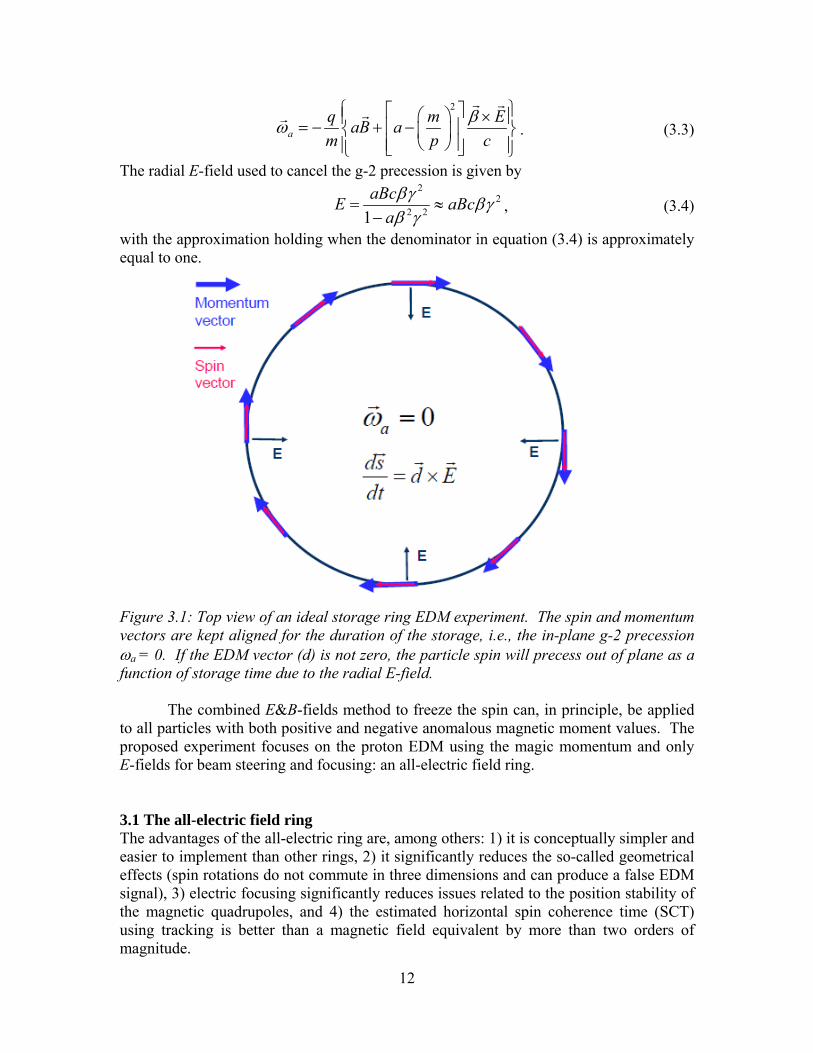
Figure 3.1: Top view of an ideal storage ring EDM experiment. The spin and momentum vectors are kept aligned for the duration of the storage, i.e., the in-plane g-2 precession a = 0. If the EDM vector (d) is not zero, the particle spin will precess out of plane as a function of storage time due to the radial E-field.

The combined E&B-fields method to freeze the spin can, in principle, be applied to all particles with both positive and negative anomalous magnetic moment values. The proposed experiment focuses on the proton EDM using the magic momentum and only E-fields for beam steering and focusing: an all-electric field ring. 3.1 The all-electric field ring The advantages of the all-electric ring are, among others: 1) it is conceptually simpler and easier to implement than other rings, 2) it significantly reduces the so-called geometrical effects (spin rotations do not commute in three dimensions and can produce a false EDM signal), 3) electric focusing significantly reduces issues related to the position stability of the magnetic quadrupoles, and 4) the estimated horizontal spin coherence time (SCT) using tracking is better than a magnetic field equivalent by more than two orders of magnitude.

13

When the focusing system is electric, the main systematic error is a net radial B-field around the ring, whereas the main one when magnetic focusing is used is a net vertical (out of plane) E-field. (The latter is described in refs. [1] and [2] and the radial B-field effect in Section 11.) In the proposed ring, counter-rotating (CR) beams will shift vertically in opposite directions in the presence of a non-zero radial B-field. The proposed beam position monitors (BPMs, see Section 9) will have enough sensitivity to reduce the radial B-field systematic error below our sensitivity limit and all but eliminate the so-called geometric effects originating from background magnetic fields.

In order to achieve enough sensitivity on the radial B-field effect, we have decided to use very weak vertical focusing (vertical tune ~0.1). This choice will also significantly increase the SCT of the stored beams. Tracking has indicated that the SCT of a simple, all-electric ring with weak focusing will be long enough to satisfy the experiment requirements with ~103 s storage time.

3.2 Basic all-electric field beam dynamics

The beam dynamics of a particle in a ring where bending is provided by a radial E-field is significantly different from the beam dynamics in a ring where the bending is provided by a vertical magnetic field. In an electric field, the kinetic energy of a particle depends on its radial position, which is not the case in magnetic rings. This dependence influences the horizontal focusing, but may leave the vertical focusing unchanged. The effect of the radial E-field was first estimated in [3] for combined magnetic and electric fields; the relevant conclusions are given in eqs. (3.5), (3.6), and (3.7), below, for an all-electric, homogenous ring with vertical focusing index m=0 (cylindrical plates). The displacement of a particle due to momentum dispersion is given by

xD Dxp R0

dp

p0

x

R0

, Dx R0, (3.5)

where x is the radial coordinate, Dx the horizontal dispersion, and R0 the ring radius. The horizontal betatron frequency depends on the particle energy

x02 1

1

02 , (3.6)

with 0 the relativistic Lorentz factor. The change of the revolution frequency depends on the momentum dispersion and the average radial position

0 0

df dp x

f p R

. (3.7)

The results of particle tracking using the Runge-Kutta integration method are consistent with eq. (3.6). Eq. (3.5) implies a maximum dp/p acceptance equal to the maximum possible x/R0 value, which in our case for x=15mm, and R0=40m, is equal to (dp/p)max =

14

3.7510-4, corresponding to ~150 keV kinetic energy. However, the momentum acceptance depends on the radial position of the particle in the interface of the straight section and E-field bending section. If a particle enters the bending section at x=0, then the momentum acceptance is only half of that implied by eq. (3.5), since the particle will oscillate past its equilibrium point (like a pendulum, it performs a simple harmonic oscillation). The radial dependence of momentum acceptance is verified by tracking. (See Appendix 4 for more results.)

3.3 Basic measurement sequence

About half of the running time will be dedicated to probing the systematic errors. The total running time is expected to be of the order of four years. The details of the running schedule are to be finalized later on as the CD process progresses. Below, we lay out the general plan for running the experiment in a way that maximizes information on the EDM signal and systematic errors.

1. Inject both CW and CCW proton beams with vertical polarization. A barrier bucket or low harmonic RF system is needed unless an E-field kicker and simultaneous injections are used.

2. Let each beam de-bunch and then re-bunch at the required frequency, using a high harmonic (h~101-102) RF-system.

3. After injecting the beam into the ring, use an RF-solenoid to rotate the spin from the vertical direction to longitudinal, producing positive and negative helicities for both the CW and CCW beams. Positive and negative helicities for both beam directions are needed to eliminate polarimeter related systematic errors.

4. Slowly drive the beam onto the target. At the polarimeter location, an aperture limiting solid target constrains the beam in both the horizontal and vertical directions. There are two efficient options to slowly drive the beam onto the target: 1) lower the vertical focusing strength, and 2) add random electric kicks to the beam, increasing its phase space. The first method can be used for the vertical direction and the second for both the vertical and horizontal directions. The proton counts scattered on the left, right, upper, and lower detectors as a function of time give information on the transverse beam polarization as a function of time (see Section 10).

5. Start the storage with a vertical tune of ~0.2. Slowly move to a vertical tune of 0.1 to drive ~40% of the beam to the polarimeter target. At early times, i.e., first ~50s, allow the spin to rotate in the horizontal plane and define the g-2 precession plane, the polarization value of the beams, and the average vertical spin component at early times.

6. Align the spin with the momentum direction as much as possible (the EDM signal sensitivity is proportional to cos, with the angle between the momentum and spin vectors). Using information from the polarimeter data, keep the proton spin as much aligned with the momentum vector as possible (limited by statistics) in both the horizontal and vertical directions. There are two possible sources for a horizontal misalignment between the spin and momentum vectors: a) a dipole magnetic field, and b) drifting of the beam momentum off its “magic” value. The

15

counter-rotating beams provide enough information to tell whether a possible misalignment source is a dipole magnetic field and/or there is a drift in the proton momentum off its “magic” value. Use ~20% of the beam during this time. Let the radial E-field act on the proton EDM for ~103 s.

7. Measure the difference between the CR beam-currents using a high sensitivity single-turn transformer to better than 0.01% on average for the duration of the storage time of ~103 s. Commercially available single turn transformers can provide this sensitivity with ~1 kHz bandwidth.

8. During the storage time, calibrate the BPM sensitivity by applying a radial B-field with amplitude of ~50pG at a frequency of our choice. This oscillating B-field will modulate the vertical separation between the counter-rotating beams with a specific amplitude for BPM calibration. In addition, modulate the vertical tune with amplitude of 10% of itself, i.e., the tune will be m=0.1+0.01×cos(ωt+) at a frequency of our choice between 101-104 Hz. In addition, apply an oscillating vertical E-field at a frequency different from the B-field modulation. The two beams will move together, but because the B-fields generated by the counter-rotating beams cancel, the BPMs should not be able to observe it. However, the button BPMs (see Appendix 8), which are sensitive to electric fields generated by the beams, should be able to see it. Monitor the vertical spin component as a function of time.

9. At late times, i.e., last ~50 s, let the spin rotate in the horizontal plane to define the g-2 precession plane, the beam polarization, and the average vertical spin component at late times. The difference between early and late times will determine the average vertical spin precession rate. In the absence of an EDM, a beam injected with a non-zero average vertical spin component will keep this component unchanged, as this is the stable spin direction.

10. At the end of storage time (or as often as needed), take the difference between the vertical spin precession rates of the beams with opposite helicity. Using feedback with a coil generating a radial B-field around the ring, keep the vertical spin precession rate as close to zero as statistics allow. (A vertical split at the vertical tune modulation indicates an EDM signal. No vertical split means the spin precession was only due to a radial B-field which we have canceled by applying a counter radial B-field.)

3.4 Basic experiment performance requirements

1. A polarized proton source, an accumulator (BOOSTER) and a transfer-line capable of delivering 2×1010 polarized protons clockwise (CW) and 2×1010 polarized protons counter-clockwise (CCW) into the EDM ring. The beam characteristics are given in Section 5.

2. A matched injection system capable of injecting the beam clockwise (CW) and counter-clockwise (CCW) into the EDM ring. The injected beam polarization is in the vertical direction.

3. State-of-the-art radial electric field plates capable of delivering ~10.5 MV/m between two parallel stainless steel plates 3 cm apart and about 20 cm high; see

16

Section 8. Refs. [4,5,6,7,8,9] below describe extensive work on achieving high electric field strengths and recent achievements in this area.

4. An RF-solenoid to precess the spin from the vertical direction to horizontal after injection. Due to polarimeter systematic error considerations, we need to have at least two bunches with opposite polarization vectors per direction.

5. An RF system that will provide a synchrotron tune of ~10-2, eliminating first-order spin de-coherence effects due to the momentum spread of the beam.

6. Sextupoles installed at strategic locations around the EDM ring to prolong the beam spin coherence time (SCT). Important work on SCT in storage rings has been done at Novosibirsk [10]. Yuri Orlov did the complete analytical work for the deuteron EDM proposal [11]; more recently, Richard Talman has done work on the all-electric proton EDM ring. Recent tracking and analytical estimations for a pure electric field and weak vertical focusing indicate a SCT well above 102s for particles with emittance parameters at the edge of the ring acceptance, even without sextupoles; see Section 6 and Appendix 4.

7. State-of-the-art internal polarimeters located in straight sections that can monitor the proton spin components as a function of time with low systematic errors. The vertical focusing is lowered slowly, driving the proton beam onto the polarimeter target, which is the limiting aperture in the ring. First-order contributions of systematic errors to the left-right asymmetry can be removed by using detection on both sides of the beam in combination with beam bunches with opposite polarizations, all combined into a cross-ratio asymmetry [12]. Furthermore, a more sophisticated cross ratio is used first to enhance and then eliminate the second-order systematic errors; see Section 10 and Appendix 7. (Our polarimeter work at COSY, described in a paper accepted for publication, showed that the anticipated systematic errors are much smaller than the expected EDM statistical resolution; see Appendix 7.)

8. State-of-the-art beam position monitors (BPMs) at most straight sections to determine the two-beam separation with high resolution; see Section 9.

9. An average radial B-field integrated around the ring below 0.15 pG, to be below our sensitivity level. The horizontal component of the earth’s B-field at the location of the ring will be of the order of 0.1G. We plan to run for about 107s, corresponding to about 104 injections, so the average radial B-field can be as much as 15 pG per storage time. The average radial B-field due to the earth’s magnetic field around the ring should be zero. But assuming (conservatively) a net field of 10 mG, we would need a shielding factor of ~109. A passive magnetic shield for the ring with a shielding factor of 104 to 105 is possible using three to four mu-metal layers [13,14]; see Sections 8 and 9. Active shielding using Helmholtz coils in the ring tunnel as well in the beam tube are assumed to provide the rest of the required shielding.

10. Elimination of the geometrical phase effect [15]. The BPM information will provide enough information to reduce the magnetic field effect contribution to geometrical phases below our statistical sensitivity level. The specs in the quality of the electric field and alignment of the plates within a section and from section to section are set by the requirements to reduce the geometrical phase effects. The relative radial position of the plates needs to be better than 30 μm; the

17

absolute position of the plates from section to section needs to be better than 30 μm; and the average E-field plane alignment needs to be better than 0.1 mrad with respect to a common plane.

11. A vacuum system capable of delivering <10-10 Torr.

Table 3.1. Parameters for the proton EDM ring.

Parameter Value Comment Proton momentum 0.700740 GeV/c Kinetic energy: 232.8 MeV,

= 0.59838, = 1.2481 Ring bending radius 40 m Total length of straight sections

11.5 m – 50 m We will leave enough straight section length for the needs of the experiment.

Radial E-field strength 10.5 MV/m For plate separation of 3 cm, the voltage on the plates is about ±160 KV.

Number of sections 16 The E-field plates within a section are each ~16m long each. If needed, they can be segmented into 5 pieces, each 3.14 m long.

Radial E-field dependence at y=0

~1/R, with the vertical field focusing index close to zero.

The E-field plates will be nearly cylindrical.

Total length of orbit 263 m – 300 m Horizontal tune 1.3 Vertical tune (weak focusing provided by quadrupoles in the straight section)

m=0.2 - 0.1 To be modulated by ~10% of itself around 0.1

Horizontal aperture 3 cm Vertical aperture 8 cm Cyclotron frequency 0.68 MHz – 0.60 MHz References

1. F.J.M. Farley et al., Phys. Rev. Lett. 93, 052001 (2004). 2. AGS Proposal: Search for a permanent electric dipole moment of the deuteron

nucleus at the 10-29 ecm level, April 2008, available at http://www.bnl.gov/edm/. 3. S.R. Mane, Nucl. Instrum. Meth. A596, 288 (2008). 4. High Voltage Technology, p. 82, Ed. By L.L. Alston, Oxford University Press

(1968).

18

5. L. Cranberg, Journ. of Appl. Phys. 23, 518 (1952). 6. D.R. Swenson et al., Nucl. Instrum. Meth. B261, 630 (2007). 7. B.M. Dunham et al., Proc. of PAC07, Albuquerque, NM, USA, 1224 (2007). 8. C.K. Sinclair, Nucl. Instrum. Meth. A557, 69 (2006); C.K. Sinclair et al., Proc. of

PAC01, Chicago, 610 (2001). 9. Vaibhav Kukreja, Field-Emission Properties in the ERL-Electron Source, Dept. of

Physics, Cornell University report (2005). 10. I.B. Vasserman et al., Phys. Lett. B187, 172 (1987); Phys. Lett. B198, 302

(1987); A.P. Lysenko et al., Part. Accel. 18, 215 (1986). 11. Yuri Orlov’s estimation of SCT included in the deuteron EDM proposal,

reference [2] and in EDM internal note #61, February 2004. 12. G.G. Ohlsen and P.W. Keaton, Jr., Nucl. Instrum. Meth. 109, 41 (1973). 13. Berlin Magnetically Shielded Room, available from:

http://www.ptb.de/cms/fileadmin/internet/fachabteilungen/abteilung_8/8.2_biosignale/8.21/mssr.pdf Bork J, Hahlbohm HD, Klein R, Schnabel, A The 8-layered magnetically shielded room of the PTB: Design and construction in Biomag2000, Proc. 12th Int. Conf. on Biomagnetism, J. Nenonen, R.J. Ilmoniemi, and T. Katila, eds. (Helsinki Univ. of Technology, Espoo, Finland, 2001), pp. 970-973

14. http://www.amuneal.com/bnlsredm1 Amuneal manufacturing corp., 4737 Darrah Street, Philadelphia, PA 19124.

15. Yuri Orlov’s estimation of the effect of consecutive rotations through perpendicular axes, included in the deuteron EDM proposal, reference [2], April 2008.

19

4. RING LATTICE FOR THE EXPERIMENT This section of the proposal primarily distills the contents of the appendices RingLat [1], UALcode [2], and LattParams [3].

4.1 Requirements imposed by the experiment

Here we discuss optimization of the ring for its experimental purpose and its adequacy as an accelerator that can store enough oriented protons for long enough. The proton EDM measurement primarily requires a purely electric radial field Er, such as shown in Figure (4.1), below. The closed orbit consists of circular arcs (joined together they would form a circle) and straight sections. Protons are stored with their spins aligned with their momenta, pointing alternately forward and backward in successive beam bunches (to cancel polarimeter related systematics). To the extent that a proton has an electric dipole moment, the EDM will be aligned along the same axis. Torque due to Er acting on EDM tips the spins up in odd bunches, and down in even ones. As each proton is extracted onto the polarimeter target, the tipping of the spin is measurable as left/right scattering asymmetry.

Figure 4.1: A purely radial electric field of the kind needed for the pEDM experiment. The bold curve shows a proton orbit passing through a curved-planar cylindrical electrostatic bending element. With these curved planar, cylindrical electrodes, the value of the electric “field index” is m=0.

Although there is only an electric field in the laboratory, there will be a vertical magnetic field By in the proton rest frame. Acting on the magnetic moment, this will create a potentially huge torque, causing the spin to precess in the horizontal plane. Fortunately, there is a “magic” momentum at which the proton spin precesses at the same

20

rate as its momentum, so the spin is “frozen” pointing parallel to the momentum. This fixes the central accelerator values as,

p 0.7 GeV/c, v

c 0.6, K 233 MeV . (4.1)

Also fortunate is the fact that the analyzing power of p-carbon elastic scattering is large at this momentum, close to 1 at the optimal angle (see Section 10).

The momentum of any particular proton will not be exactly magic, so its spin will precess away from longitudinal. Because of energy spread, the spins will decohere. Since the optimal run length will be about 103 seconds, the spin coherence time (SCT) must be increased. This is one of the issues governing the design of the lattice. Finite betatron amplitudes also contribute to SCT. These effects can be reduced by appropriate linear lattice design, and further reduced using sextupoles.

Radial magnetic field Br acting on magnetic dipole moment (MDM) mimics the effect of EDM. Since even the best achievable magnetic shielding may not be sufficient, further measures must be taken against systematic error caused by Br. One is to store counter-rotating proton beams. By time reversal invariance, electric fields cause counter-circulating orbits to be identical. But non-zero Br separates the beams vertically. This separation depends inversely on the vertical tune. It is this dependence that demands a small value for the vertical tune Qy. With their beam currents matched by nulling a wall current monitor or single turn transformer, this separation can be measured and then nulled by an active Br coil. A bonus from small Qy is reduced contribution to spin decoherence of vertical betatron oscillations.

For the anticipated beam currents, precision greater than that provided by a conventional button beam position monitor (BPM) is needed to measure the DC offset of counter-circulating beams. By modulating the vertical tune Qy, the vertical separation can be measured much more accurately using lock-in, synchronous detection.

The relative vertical displacement of the opposing beams produces radial magnetic fields in the design plane. Measuring this beam-induced Br with SQUID magnetometers will give further needed precision. There is also a vertical signal By above and below, but the sensitivity for measuring it is lower there. Finally, statistical errors will be addressed by averaging the results of a great many runs.

4.2 Implications of electric (rather than magnetic) bending

The proposed electrostatic storage ring will be more than ten times larger than any previous electrostatic ring [4,5,6]. In spite of this, its betatron tunes will be less than any of these earlier rings. Because of their strong focusing, beam dynamics in these predecessor rings scarcely distinguished between electric and magnetic dynamics. (In fact, the AGS-Analog ring built at BNL was regarded as a prototype for the magnetic AGS [4].) The main challenges for the EDM ring will be precision vertical beam position monitoring and achieving adequately long SCT, both of which favor extremely low tune values. These values amplify the differences between electric and magnetic focusing. The differences are due to the variation of particle speed in electric, but not

21

magnetic, fields. In addition to the challenge of spin polarization conservation, these differences impose other special operational challenges, especially for injection.

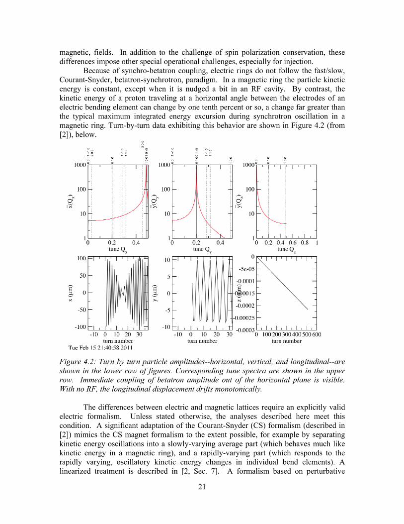
Because of synchro-betatron coupling, electric rings do not follow the fast/slow, Courant-Snyder, betatron-synchrotron, paradigm. In a magnetic ring the particle kinetic energy is constant, except when it is nudged a bit in an RF cavity. By contrast, the kinetic energy of a proton traveling at a horizontal angle between the electrodes of an electric bending element can change by one tenth percent or so, a change far greater than the typical maximum integrated energy excursion during synchrotron oscillation in a magnetic ring. Turn-by-turn data exhibiting this behavior are shown in Figure 4.2 (from [2]), below.

Figure 4.2: Turn by turn particle amplitudes--horizontal, vertical, and longitudinal--are shown in the lower row of figures. Corresponding tune spectra are shown in the upper row. Immediate coupling of betatron amplitude out of the horizontal plane is visible. With no RF, the longitudinal displacement drifts monotonically.

The differences between electric and magnetic lattices require an explicitly valid

electric formalism. Unless stated otherwise, the analyses described here meet this condition. A significant adaptation of the Courant-Snyder (CS) formalism (described in [2]) mimics the CS magnet formalism to the extent possible, for example by separating kinetic energy oscillations into a slowly-varying average part (which behaves much like kinetic energy in a magnetic ring), and a rapidly-varying part (which responds to the rapidly varying, oscillatory kinetic energy changes in individual bend elements). A linearized treatment is described in [2, Sec. 7]. A formalism based on perturbative

22

treatment in the m=0, cylindrical electrode case is described in [2, Sec. 3]. Though partially implemented, this approach has been superseded by the following, better controlled method in preparation for long-term, symplectic tracking: an exact formalism (described in [2, Sec. 4]) based on a generalized Hamilton vector for Coulomb's law 1/r2 electric field variation. This formalism, developed for relativistic atomic theory and cosmology by Munoz and Pavic, was discovered by John Talman, who has adapted it for the UAL/ETEAPOT code for this experiment.

A bend/kick/bend algorithm is used for particle tracking. Deviations of the actual field index m from its Coulomb field value (m=1) are handled by (symplectic) kicks. This approach becomes increasingly precise as the bend element slicing is made finer. From the time of its inception, the “nominal” electric field dependence has been taken to be the 1/r, m=0 dependence between cylindrical plates. A proof that m=0 is optimal from the point of view of long SCT is contained in [1, Sec. 6]. (Based on a virial theorem, this demonstration is nonperturbative and direct. The theorem is applicable, however, only to uniform rings without straight sections. It does not, therefore, weigh in on the extent to which very long straight sections contribute to spin decoherence.)

Matching the centripetal force required for circular motion, to the actual electric field, Newton's law gives

mpv2

r

eE0

r1m (4.2)

For m=0 the factors of r cancel and the particle speed is independent of radius. The choice m=0 leads to an optimally long SCT. This means that in order to have vertical focusing one must run “close to” m=0 for long SCT, but far enough away from m=0 for stable accelerator operation. Development of the simulation code that will be needed for these delicate matters is described in [2].

4.3 Lattice design considerations

The current lattice design, along with a chronology of its development, is described in [1]. Parameters for the two most up-to-date storage ring EDM lattices are given in [3]. (Documentation for earlier versions is available if needed.) These two latest “test lattices” are referred to as LSCT (Long Spin Coherence Time) and SC (Stochastic Cooling). The LSCT name was based on analysis assuming a condition carried over from magnetic formalism. The SC ring is intended for studies of stochastic cooling.

The SC lattice is somewhat more practical than the LSCT lattice in one respect: its straight sections are amply long (~50 m) for the sorts of control, measurement, feedback, and magnetic shielding equipment that will be needed whether or not stochastic cooling is feasible.

Stabilization of the frozen-spin configuration by RF focusing is especially important. The longitudinal focusing has to be at least strong enough to keep the wandering of the proton axis away from the frozen spin direction within reasonable bounds (certainly much less than π/2). Beyond this, further increase of RF voltage may be counter-productive because of the possibility of resonant-depolarization.

23

Straight sections have been made available for practical injection, RF, polarimetry, and so on. It is usually considered desirable to have dispersion suppression at the ends of major arcs, but this has not been possible for the low tune values we need. This makes the racetrack configuration less attractive. Considerations of simplicity and superior spin coherence time favor a near-circular ring. The need to minimize the total length of all straight sections requires BPM, quadrupole, and sextupole lengths to be minimized. Then the need for a few longer elements, in particular polarimeter and injection hardware, requires two “long” (still only about 2 m long) straightaway sections in a racetrack geometry.

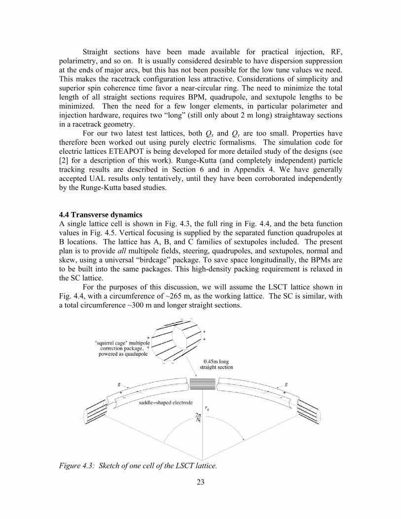
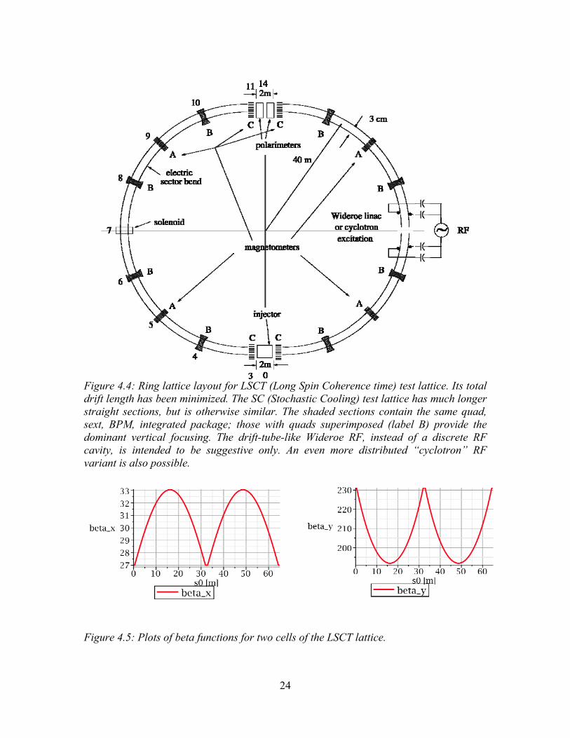
For our two latest test lattices, both Qx and Qy are too small. Properties have therefore been worked out using purely electric formalisms. The simulation code for electric lattices ETEAPOT is being developed for more detailed study of the designs (see [2] for a description of this work). Runge-Kutta (and completely independent) particle tracking results are described in Section 6 and in Appendix 4. We have generally accepted UAL results only tentatively, until they have been corroborated independently by the Runge-Kutta based studies. 4.4 Transverse dynamics A single lattice cell is shown in Fig. 4.3, the full ring in Fig. 4.4, and the beta function values in Fig. 4.5. Vertical focusing is supplied by the separated function quadrupoles at B locations. The lattice has A, B, and C families of sextupoles included. The present plan is to provide all multipole fields, steering, quadrupoles, and sextupoles, normal and skew, using a universal “birdcage” package. To save space longitudinally, the BPMs are to be built into the same packages. This high-density packing requirement is relaxed in the SC lattice. For the purposes of this discussion, we will assume the LSCT lattice shown in Fig. 4.4, with a circumference of ~265 m, as the working lattice. The SC is similar, with a total circumference ~300 m and longer straight sections.

Figure 4.3: Sketch of one cell of the LSCT lattice.

24

Figure 4.4: Ring lattice layout for LSCT (Long Spin Coherence time) test lattice. Its total drift length has been minimized. The SC (Stochastic Cooling) test lattice has much longer straight sections, but is otherwise similar. The shaded sections contain the same quad, sext, BPM, integrated package; those with quads superimposed (label B) provide the dominant vertical focusing. The drift-tube-like Wideroe RF, instead of a discrete RF cavity, is intended to be suggestive only. An even more distributed “cyclotron” RF variant is also possible.

Figure 4.5: Plots of beta functions for two cells of the LSCT lattice.

25

4.5 Injection While the requirement of using only electric fields for the EDM experiment means that the electric deflection will be weaker than that achievable by a magnetic deflection, it has an important advantage: deflection hardware has negligible “inertia.” It is the capacitance of sector bend elements that constitutes the inertia. With R0=40 m, the length of a sector bending through 2π/16=400 mr is about 15 m. With gap g=0.03 m and electrode height 0.2 m, the capacity has a (very small) value,

C2 /16 1011 15 0.2

0.031.1 nF. (4.3)

A sketch of a possible injection scheme is shown in Fig. 4.6. Just before injection, the injected beam inclination is Δθ. The detailed design depends on the value of Δθ.

Figure 4.6: Rough schematic illustrating the use of the electrodes of one sector bend as one element of the injection inflector. The total deflection has to be great enough to prevent protons from following the broken line, to be lost on the inner electrode.

For a single electric inflector to be sufficient, it would be necessary to apply the inflector pulse to a quite short Linfl. ~ 2 m electrode section, such as shown in the figure. 50 kV inflector pulses would be adequate and physically possible, though challenging. With purely electric inflection it would be possible to inject counter-circulating beams simultaneously. With magnetic inflection the injections have to be staggered in time.

26

Injection into the proton EDM ring shares many requirements with injection into the muon g-2 experiment ring, the most important being that magnetic materials are not allowed. Magnetic deflection would therefore require air core coils. Comparison of the required parameters for the EDM experiment and those for the muon g-2 inflector [1, Table 7] show that those for the EDM experiment are less demanding.

References

1. R. Talman, Ring Lattice for the Proton EDM Experiment, Appendix (1) to current proposal.

2. N. Malitsky, J. Talman, and R. Talman, Development of the UAL/ETEAPOT Code for the Proton EDM Experiment, Appendix (2) to current proposal.

3. R. Talman, Lattice Parameters for the Proton EDM Experiment, Appendix (3) to current proposal.

4. M. Plotkin, The Brookhaven Electron Analog, 1953-1957, BNL-45058, 1991. 5. S. Moller, ELISA, an Electrostatic Storage Ring for Atomic Physics, Nucl.

Instrum. Meth. A394, p. 281, 1997. 6. T. Tanabe, et al., An Electrostatic Storage Ring for Atomic and Molecular

Science, Nucl. Instrum. Meth. A482, p. 595, 2002.

27

5. BEAM PARAMETERS AT BNL Given the current parameters of the EDM ring, it is desirable to have a small horizontal beam size in the location of the plates. Currently, the full distance between the plates is 30 mm. The ring lattice is currently under development. (See Section 3 for a discussion of the dispersion for a fully electrostatic lattice.) Assuming a maximum dispersion function of Dx=25 m, rms momentum spread 210-4, maximum horizontal beta function of h=28m, and emittance of 3 mm mrad (95%, unnormalized), the horizontal rms beam size is 6.2 mm. The horizontal aperture between the plates can thus accommodate 2.4 of the beam. Such transverse acceptance is marginal, but could be sufficient for beam injection from the AGS with minimum beam losses. The required beam lifetime in the EDM ring is relatively short, since the beam will be constantly lost on the target as part of the experiment. The maximum allowed horizontal emittance of the beam is 3 m (95%, unnormalized), which corresponds to 2.2 m (95%, normalized) for this energy. The values of normalized emittance are obtained by multiplying the unnormalized value by the relativistic factor . The contribution to the horizontal beam size from the dispersive term is significant, and a smaller momentum spread of the injected beam would help. However, obtaining a smaller momentum spread would require use of electron cooling in the AGS (which is possible) and would increase beam dimension growth due to intra-beam scattering (IBS) in the EDM ring unless the beam intensity were decreased. Therefore, it is currently assumed that an rms momentum spread of 210-4 will be satisfactory. Further development of the lattice may result in smaller values of the dispersion function, which will help as well.

The BNL booster ring will be used to prepare the required bunches for transport in the EDM ring. These bunches will then be transported through the AGS, with the AGS being used as a transport channel. The required kinetic energy for protons is 233 MeV, which is slightly above the current 200 MeV injection energy of the Booster. At this energy, the expected polarization is determined by the polarized source performance, which at present is 80%. After the planned upgrade of the source in 2012, it is expected that the polarization will be increased to about 90%. Below is a summery of the needed and available beam injection parameters: Beam parameters needed for injection into the proposed EDM ring Single bunch intensity: 21010 Horizontal emittance (95%, normalized): 2 mm mrad Vertical emittance (95%, normalized): 6 mm mrad Rms momentum spread: 210-4 Beam parameters currently available from the Booster Bunch intensity: 21011 Transverse emittances (x and y): 6 mm mrad Rms momentum spread: 510-4

28

The available horizontal emittance from the Booster is a factor of 3 larger than needed for the EDM ring. However, the maximum allowable intensity in a single bunch due to collective effects (such as IBS) in the EDM ring is about one order of magnitude smaller. Thus, the Booster will be used to collimate bunches to the required emittance of 2 m (95%, normalized). The momentum spread will also be reduced to the required value at the expense of the beam intensity. This seems to be doable, since we are allowed to lose about a factor of 10 in single bunch intensity. Pre-cooling of proton bunches to get a smaller momentum spread, studied by us in the past, is possible. However, we currently do not anticipate the need for such pre-cooling, since scraping can produce the required beam parameters.

After long bunches of the necessary intensity, emittance and momentum spread are prepared in the Booster, they will be transported through the AGS ring and injected into the EDM ring. As described earlier, the bunches in the EDM ring will be captured either by a barrier bucket RF or a low-frequency RF system. A long bunch with 21010 vertically polarized protons will be injected into the EDM ring clockwise (CW) and another one counter-clockwise (CCW). The beam will then be de-bunched. To produce high synchrotron tune values, bunches will then be captured into the high frequency RF. We currently assume h=102 RF (70 MHz system) and synchrotron tune Qs~0.01. At the start of the experiment there will be 102 short bunches rotating CW and 102 short bunches rotating CCW. The individual bunch intensity is currently 2×108 or the total intensity of all 200 bunches 4×1010. The polarization is rotated from the vertical to the horizontal plane with an RF solenoid at the revolution frequency 0.6-0.7MHz. Ideally the waveform is a “square wave” to get two polarization states for each of the CW/CCW beams.

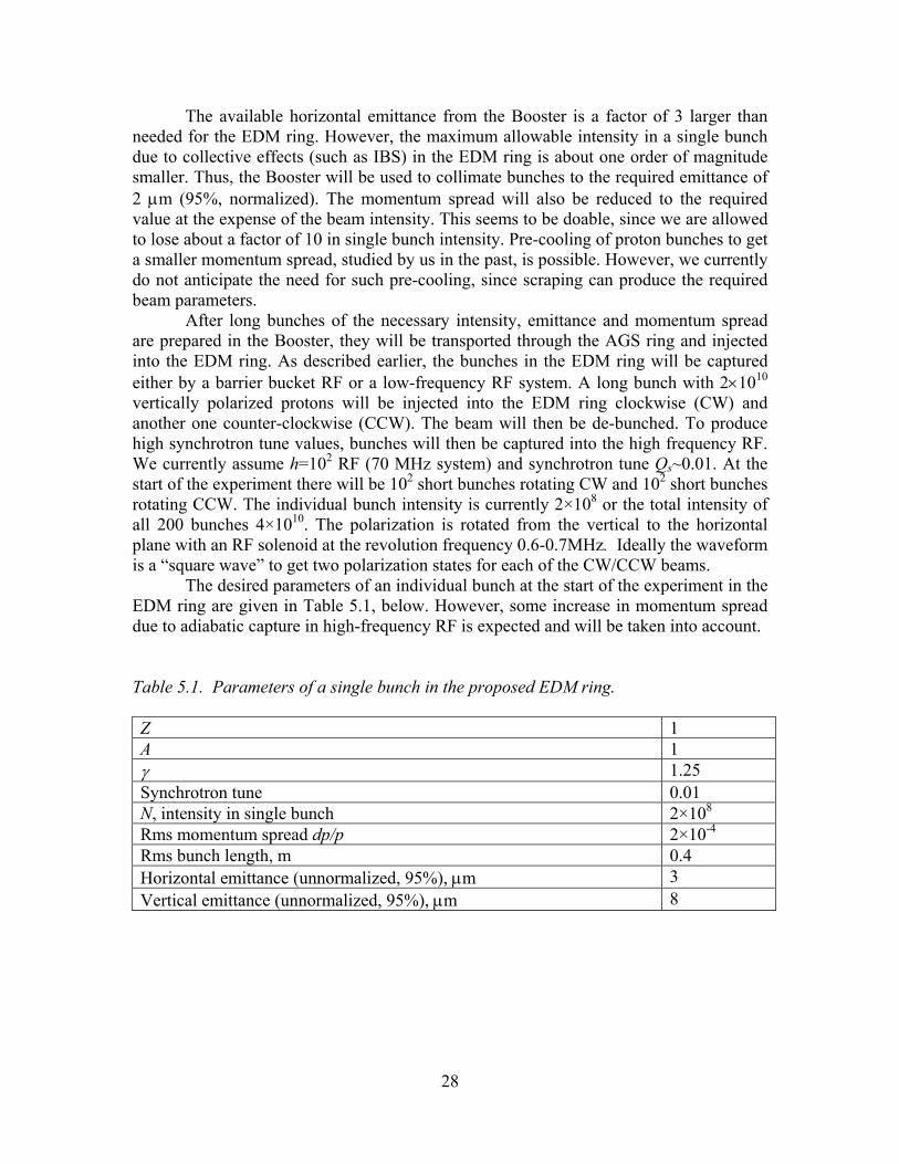
The desired parameters of an individual bunch at the start of the experiment in the EDM ring are given in Table 5.1, below. However, some increase in momentum spread due to adiabatic capture in high-frequency RF is expected and will be taken into account. Table 5.1. Parameters of a single bunch in the proposed EDM ring. Z 1 A 1 1.25 Synchrotron tune 0.01 N, intensity in single bunch 2×108

Rms momentum spread dp/p 2×10-4 Rms bunch length, m 0.4 Horizontal emittance (unnormalized, 95%), m 3 Vertical emittance (unnormalized, 95%), m 8

29

6. BEAM AND SPIN TRACKING SIMULATIONS The simulations need to take into account the various effects of beam and spin dynamics to at least the second-order. When describing the particle motion in an electric field, they also need to take into account the fact that particle momentum changes as a result of particle motion in the E-field region. The collaboration has already developed or is developing simulation programs that accurately describe the beam and spin dynamics of a particle in a storage ring. Below is a summary of its three major efforts:

1. A particle-tracking program that uses numerical integration methods (like 4th-order Runge-Kutta) to integrate beam and spin dynamics differential equations. (Similar methods have been used to describe the beam and spin dynamics for the muon g-2 experiment.) The program has been benchmarked to high accuracy for magnetic fields, where second-order effects can be estimated analytically. Benchmarking for storage rings with radial electric fields has also been done for effects that can be estimated analytically, e.g., horizontal tunes as a function of the E-field shape in the horizontal plane. This method [1] uses definitions of E and B-fields as a function of position so that, in principle, it can be accurate to a very high order. A typical step size is 0.5-1 ps, making it quite slow; a few ms in the ring typically take a few hours to simulate.

2. An update of a very efficient simulation program, used around the world to track particles in magnetic fields. This program, based on transfer matrices, has been updated to include the required high-order effects and benchmarked for storage rings, which are dominated by magnetic fields. The beam dynamics is provided by UAL/TEAPOT and the spin dynamics by UAL-SPINK. This program is currently being used to describe the deuteron beam and spin dynamics at COSY for the needs of the SCT tests.

3. A new method based on UAL/ETEAPOT [2], to take into account the momentum change of the particle due to motion in the E-fields. Preliminary results show that the gain in speed could be as much as 106 over the 4th-order Runge-Kutta method, making the particle simulation for the duration of the storage feasible. The method is still under development; see section 4 and Appendix 2. Other efforts based on numerical integration are also being considered by the

collaboration for use in EDM studies, for example Zgoubi, and simulations based on 4th-order Runge-Kutta integration (see Appendix 4) that show the SCT predictions in an all-electric field ring, where vertical focusing is provided by shaping the vertical E-field plates. (Below, we show limited simulations using the latter). COSY-infinity [3] is used in parallel at the Institute for Nuclear Physics of the Forschungszentrum at Jülich. As they mature, all the above-mentioned efforts need to be cross-checked for benchmarking.

30

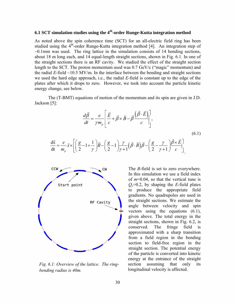
6.1 SCT simulation studies using the 4th-order Runge-Kutta integration method

As noted above the spin coherence time (SCT) for an all-electric field ring has been studied using the 4th-order Runge-Kutta integration method [4]. An integration step of ~0.1mm was used. The ring lattice in the simulation consists of 14 bending sections, about 18 m long each, and 14 equal-length straight sections, shown in Fig. 6.1. In one of the straight sections there is an RF cavity. We studied the effect of the straight section length to the SCT. The proton momentum used was 0.7 GeV/c (“magic” momentum) and the radial E-field ~10.5 MV/m. In the interface between the bending and straight sections we used the hard edge approach, i.e., the radial E-field is constant up to the edge of the plates after which it drops to zero. However, we took into account the particle kinetic energy change, see below.

The (T-BMT) equations of motion of the momentum and its spin are given in J.D. Jackson [5]:

,

p

Ed e EB

dt m c c

(6.1)

ds 11 1

dt 2 2 1 2 1p

e g g g Es B B

m c

.

The B-field is set to zero everywhere. In this simulation we use a field index of m=0.04, so that the vertical tune is Qy=0.2, by shaping the E-field plates to produce the appropriate field gradients. No quadrupoles are used in the straight sections. We estimate the angle between velocity and spin vectors using the equations (6.1), given above. The total energy in the straight sections, shown in Fig. 6.2, is conserved. The fringe field is approximated with a sharp transition from a field region in the bending section to field-free region in the straight section. The potential energy of the particle is converted into kinetic energy at the entrance of the straight section assuming that only its longitudinal velocity is affected.

Fig. 6.1: Overview of the lattice. The ring-bending radius is 40m.

31

The particle moves in the straight section with no force acting on it. If there is RF in the straight section, the energy is changed by an amount of V=Vrfcos(ωt+φ) at the RF-location. Again, only the longitudinal velocity is changed due to this energy change.

When the particle enters the bending section, its energy is shared by kinetic and potential energy, according to its position. For example, a particle at 1.5 cm from the design orbit has a potential energy of about 150 keV. This roughly corresponds to ∆p/p0=3.5×10-4, and therefore is significant.

The tracking program used is elementary, very accurate, and at the same time quite slow. The integration method used is fourth-order Runge-Kutta: to obtain the required accuracy, the step size is kept at ~1ps. It takes several hours to track a particle for 10 ms, i.e., about 104 turns. A similar program based on the

same technique, used to track muons for the needs of the muon g-2 experiment, accurately reproduced second-order effects originating from the so-called pitch effect (vertical oscillations) and the presence of E-fields and muon momentum dispersion. Those effects were estimated analytically, compared with tracking results, and found to be the same to the 10-8 level.

In the all-electric field case, the program reproduces the modified horizontal tunes (as estimated independently and using different methods, by S. Mane [6] and Yuri Orlov) that result from coupling between the radial position and particle kinetic energy. 6.2 Simulation studies of the effect of straight section length on SCT

Simulation studies of how straight section length influences SCT have been done for 14 cm, 14 m, 28 m, and 49 m of total straight section lengths. In these simulations, the initial z0 (vertical coordinate) and x0 (radial coordinate) were kept to zero while the initial momentum deviation was ∆p/p=2×10-4 off the magic momentum for all straight section lengths.

Fig. 6.2: Sketch of a straight section in the ring. The proton potential energy in the straight section is zero, while its total energy (kinetic plus potential) is constant everywhere.

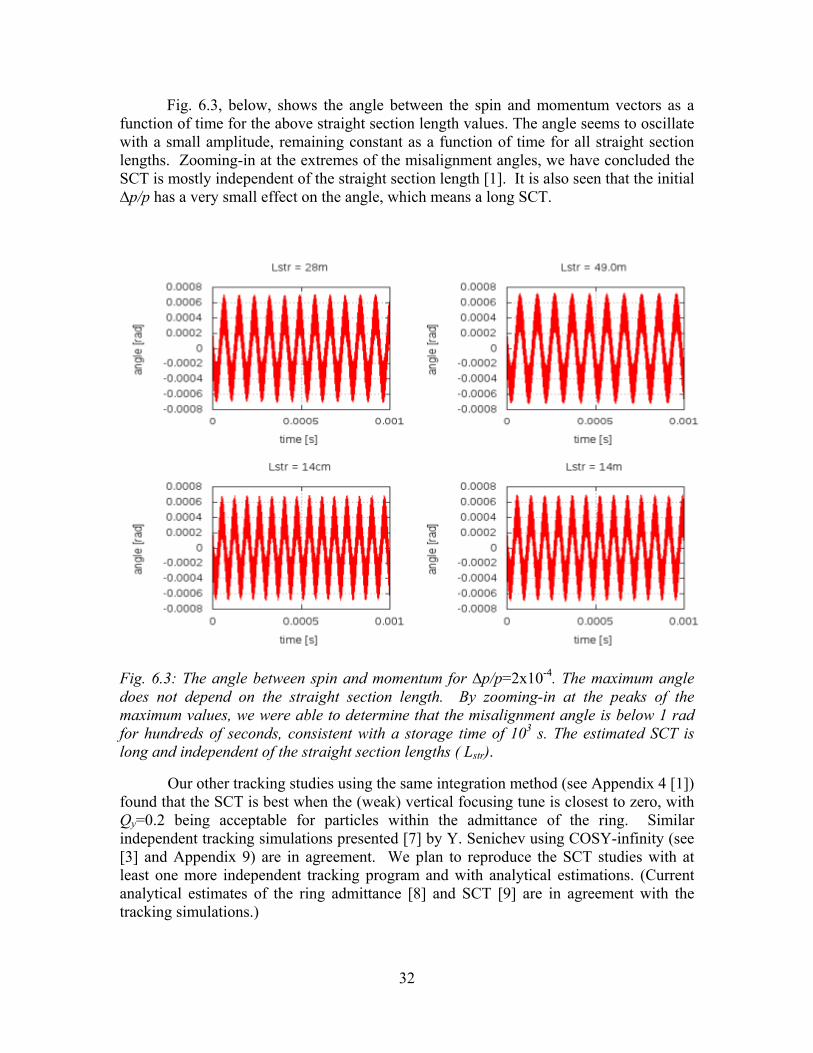
32

Fig. 6.3, below, shows the angle between the spin and momentum vectors as a function of time for the above straight section length values. The angle seems to oscillate with a small amplitude, remaining constant as a function of time for all straight section lengths. Zooming-in at the extremes of the misalignment angles, we have concluded the SCT is mostly independent of the straight section length [1]. It is also seen that the initial ∆p/p has a very small effect on the angle, which means a long SCT.

Fig. 6.3: The angle between spin and momentum for ∆p/p=2x10-4. The maximum angle does not depend on the straight section length. By zooming-in at the peaks of the maximum values, we were able to determine that the misalignment angle is below 1 rad for hundreds of seconds, consistent with a storage time of 103 s. The estimated SCT is long and independent of the straight section lengths ( Lstr).

Our other tracking studies using the same integration method (see Appendix 4 [1]) found that the SCT is best when the (weak) vertical focusing tune is closest to zero, with Qy=0.2 being acceptable for particles within the admittance of the ring. Similar independent tracking simulations presented [7] by Y. Senichev using COSY-infinity (see [3] and Appendix 9) are in agreement. We plan to reproduce the SCT studies with at least one more independent tracking program and with analytical estimations. (Current analytical estimates of the ring admittance [8] and SCT [9] are in agreement with the tracking simulations.)

33

The conclusions we have drawn from the above studies are:

The SCT is >103 s with RF-on for particles in a continuous, ideal, all-electric ring with R~40 m, and plate separation 3cm. The larger the radius, the better the SCT.

With RF-on in a ring with straight sections, 1 mrad horizontal angular deviation does not produce a measurable deterioration of the SCT.

A particle with dp/p=2×10-4 (at the edge of the ring acceptance) gives a misalignment angle between spin and momentum vectors below 1 rad for hundreds of seconds, allowing a storage time of >103s. It has a very weak dependence on the straight section length, making space available for more diagnostic equipment in case of need. Particles with large dp/p can be taken out at earlier times in the storage period, while those with smaller emittances can be stored for longer times.

A particle starting at a vertical offset of 2 cm produces a misalignment angle with respect to an ideal one, with a rate of 1.6 mrad/s for almost no straight section length and 4 mrad/s for 49 m of total straight section length. Again, those particles will be taken out at the polarimeter detector earlier in the storage time.

If the E-field is constant with respect to radius, the SCT deterioration will be 250 mrad/s, see (Y1) graph in Fig. 11 of the appendix 4, when dp/p=2×10-4. When the ~1/R nature of the E-field is taken into account, the long SCT is restored, see (Y4) and (theta) graphs of the same figure. This means that the field-focusing index closest to zero gives the best SCT values, with a vertical tune of 0.2 being satisfactory.

Given the correlation between radial position and particle energy, the traditional ring admittance means slightly different things in the all-electric field case. We found that horizontally we can store particles with dp/p ~2×10-4 and x~0.4mrad, which corresponds to about 5 mm mrad horizontal admittance. However, the admittance of this ring depends on the injection method due to the coupling between the radial position and its energy [1].

Another important development is the understanding of intensity limitations of the ELISA ring at the University of Aarus Denmark [10], as reported by Alexander Papash [11]. Running BETACOOL, they were able to duplicate the observed stored beam intensity of 22 KeV O- as a function of storage time. The very large voltage difference between the electric field plates divided by the particle kinetic energy in the ELISA ring (±10-1), coupled with the large non-linear E-fields in the bending sections, is believed to have played a significant role in the losses with increased beam intensity. Even though the corresponding parameters for the proton EDM ring are much more advantageous, making it much less susceptible to those losses, more detailed tracking studies are needed to establish the dynamic aperture of the ring.

Currently we have adopted as a working lattice the simple lattice shown in Fig. 4.4. The total length of the straight sections is not finalized at this point, but we will assume it to be between 11.5 m (LSCT lattice) and 50 m (SC lattice). Alternative lattices are also being worked on and we intend to finalize its basic design by the time we apply for CD1.

34

References

1. S. Haciomeroglu and Y.K. Semertzidis, SCT with 4th-Order Runge-Kutta Simulations, Appendix 4 to this proposal.

2. N. Malitsky, J. Talman, and R. Talman, Development of the UAL/ETEAPOT Code for the Proton EDM Experiment, UALcode, Appendix 2 to this proposal.

3. COSY-Infinity is a particle tracking program available from the Michigan State University web site: http://bt.pa.msu.edu/index_cosy.htm.

4. W.H. Press, S.A. Teukolsky, W.T. Vetterling, Numerical Recipes, 2007. 5. J.D. Jackson, Classical Electrodynamics, 2nd ed., 1975. 6. S. Mane, Nucl. Instrum. Meth. A596, 288 (2008). 7. Y. Senichev’s Features of beam dynamics in electro-static rings presentation at

Search for EDMs at Storage Rings, 485. WE-Heraeus-Seminar, Bad Honnef, July 2011. Available at http://www2.fz-juelich.de/ikp/edm/en/program.shtml.

8. William Morse, EDM internal note on beam dynamics in electro-static rings, June 2011.

9. Yuri Orlov, EDM internal note on SCT, September 2010. 10. S.P. Moeller et al., proceedings of EPAC 2000, Vienna, Austria, p. 788; S.P.

Moeller’s The low energy storage ring ELISA and her younger sister, presentation at Search for EDMs at Storage Rings, 485. WE-Heraeus-Seminar, Bad Honnef, July 2011. Available at http://www2.fz-juelich.de/ikp/edm/en/program.shtml.

11. A. Papash’s Ultra-low energy Storage Ring (USR) at FLAIR, presentation at Search for EDMs at Storage Rings, 485. WE-Heraeus-Seminar, Bad Honnef, July 2011. Available at http://www2.fz-juelich.de/ikp/edm/en/program.shtml.

35

7. SPIN COHERENCE TIME EXPERIMENT

7.1 Overview The signal for an electric dipole moment (EDM) is the rotation of the polarization away from the longitudinal (parallel to the beam velocity) direction and toward the vertical direction under the influence of radial electric fields in a storage ring. The polarization component in the vertical direction is generally stable for a ring in the horizontal plane. But the electric or magnetic fields that hold the beam in the ring also cause any polarization component in the plane to precess. The rate of precession, or spin tune, is defined relative to the cyclotron frequency. Small position or speed variations among the beam particles give rise to a spread in spin tunes and eventual decoherence, resulting in a loss of polarization and EDM signal.

The largest first-order contribution to decoherence, the momentum spread Δp/p, can be corrected simply by imposing a beam bunch structure with an RF cavity that forces all particles to follow the same rotation rate on average. However, there are further effects that vary as the square of a small variation. Large synchrotron oscillations are accompanied by beam particles that spend a long time well away from the central momentum. Any effect that depends on (Δp/p)2 will accumulate. Likewise, betatron oscillations with a finite emittance will give rise to a class of particles whose average momentum is slightly higher than the central value, since they must follow a longer path and complete a revolution around the ring in the same time as the central particle. This contribution to the path length increase is often parameterized in terms of the square of the maximum angle that the oscillating particle has with respect to the beam direction, either ΘX

2 or ΘY2.

One effect of sextupole fields in conjunction with quadrupole focusing fields is a shift of the particle orbit away from the central axis that depends on a particle’s value of ΘX

2 or ΘY2 [1]. The purpose of this study is to determine whether such shifts can be used

effectively to reduce or eliminate the decohering due to the emittance and momentum spread. Other handles may be available as well. Beam cooling, either in the form of electron cooling before injection into the EDM ring or stochastic cooling during the store, could be used directly to reduce the size of the emittance and momentum spread. Shaping of the RF cavity voltage, as is often done to prepare particularly long beam bunches for experiments, may also be used to modify the response to momentum spread.

The design of this study contains three major steps built upon the success with the EDDA scintillator array in providing a continuous polarimeter that can track polarization changes throughout the beam store:

(a) An RF-solenoid already installed at COSY is used to excite the 1-G spin resonance for a deuteron beam (see Section 10). The width of this resonance depends on the same emittance and momentum spread parameters as the spin coherence lifetime. The first run in January 2011 was an attempt to observe these depolarizing effects. These data, along with measurements of the beam and machine properties, will form the basis for commissioning spin-tracking calculations based on a detailed model of the COSY ring lattice.

(b) The EDDA polarimeter electronics will be improved to record a time stamp for every event so that the g-2 rotation of the in-plane polarization can be followed explicitly in the data. For this, a simulation of the ring is needed to

36

determine the best method for producing a horizontally polarized beam using the RF-solenoid.

(c) Once the horizontal polarization measurement capability is established, future spin tracking calculations of the horizontal polarization lifetime will be used to adjust the sextupole fields in order to reduce or eliminate the decoherence produced by emittance and momentum spread.

The COSY Program Advisory Committee has recently approved beam time for the second of these runs, which will occur sometime between November 2011 and May 2012. 7.2 Preliminary results from the January 2011 run Expecting that simple momentum spread would produce too large a decoherence, we made all measurements with the beam bunched on the first harmonic. The RF-solenoid was then used to create a series of fixed and variable frequency scans in the neighborhood of the spin resonance with an uncooled and an electron-cooled beam, different RF-solenoid strengths, and different patterns of on and off times. In addition, various attempts were made to use white noise to heat the horizontal phase space and to adjust the strength of one of the sextupole magnet families. In parallel, measurements were made of the ring steering and focusing response matrices; the cooled and uncooled beam profiles; the slip factor; the compaction factor; and the distribution of strength in the Schottky spectrum. The initial analysis was conducted by comparing the time dependence of the polarization under various conditions with a simple model containing only the g-2 and RF-solenoid rotations. Through detailed and successful comparisons with the data, this model revealed that essentially all of the phenomena observed during the run could be related directly to the effects of time slip relative to the RF-solenoid for particles undergoing large synchrotron oscillations. Such models are sensitive to, and yield information about, the spatial distribution of particles within the beam bunch. The variety of effects observed is rich and worthy of analysis in its own right. No effects were observed that could clearly be attributed to either momentum spread or emittance. These processes were included in the simple model through a consideration of path lengthening, and found to be small and generally indistinguishable from subtle variations in the larger effects of synchrotron oscillations. Circumstantial evidence exists for a lower limit of about one minute on the horizontal spin coherence time of the deuteron beam when the beam is electron-cooled. Further study of emittance and momentum spread effects will be made after the commissioning of direct horizontal polarization measurements, since this will no longer require the use of the RF-solenoid to perform any task other than polarization preparation. References

1. Y. Orlov, EDM internal note 61, February 2004.

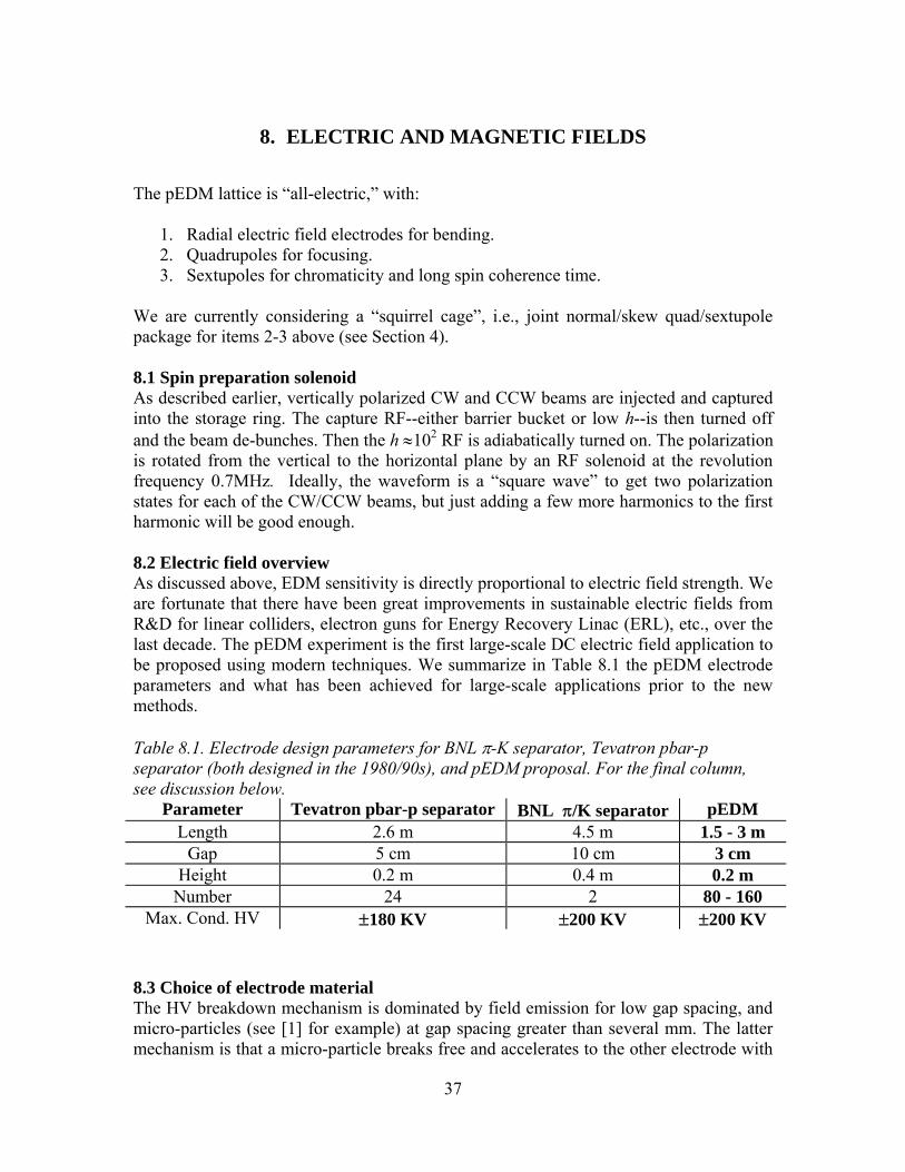
37

8. ELECTRIC AND MAGNETIC FIELDS

The pEDM lattice is “all-electric,” with:

1. Radial electric field electrodes for bending. 2. Quadrupoles for focusing. 3. Sextupoles for chromaticity and long spin coherence time.

We are currently considering a “squirrel cage”, i.e., joint normal/skew quad/sextupole package for items 2-3 above (see Section 4). 8.1 Spin preparation solenoid As described earlier, vertically polarized CW and CCW beams are injected and captured into the storage ring. The capture RF--either barrier bucket or low h--is then turned off and the beam de-bunches. Then the h 102 RF is adiabatically turned on. The polarization is rotated from the vertical to the horizontal plane by an RF solenoid at the revolution frequency 0.7MHz. Ideally, the waveform is a “square wave” to get two polarization states for each of the CW/CCW beams, but just adding a few more harmonics to the first harmonic will be good enough. 8.2 Electric field overview As discussed above, EDM sensitivity is directly proportional to electric field strength. We are fortunate that there have been great improvements in sustainable electric fields from R&D for linear colliders, electron guns for Energy Recovery Linac (ERL), etc., over the last decade. The pEDM experiment is the first large-scale DC electric field application to be proposed using modern techniques. We summarize in Table 8.1 the pEDM electrode parameters and what has been achieved for large-scale applications prior to the new methods. Table 8.1. Electrode design parameters for BNL -K separator, Tevatron pbar-p separator (both designed in the 1980/90s), and pEDM proposal. For the final column, see discussion below.

Parameter Tevatron pbar-p separator BNL /K separator pEDM Length 2.6 m 4.5 m 1.5 - 3 m

Gap 5 cm 10 cm 3 cm Height 0.2 m 0.4 m 0.2 m

Number 24 2 80 - 160 Max. Cond. HV 180 KV 200 KV 200 KV

8.3 Choice of electrode material The HV breakdown mechanism is dominated by field emission for low gap spacing, and micro-particles (see [1] for example) at gap spacing greater than several mm. The latter mechanism is that a micro-particle breaks free and accelerates to the other electrode with

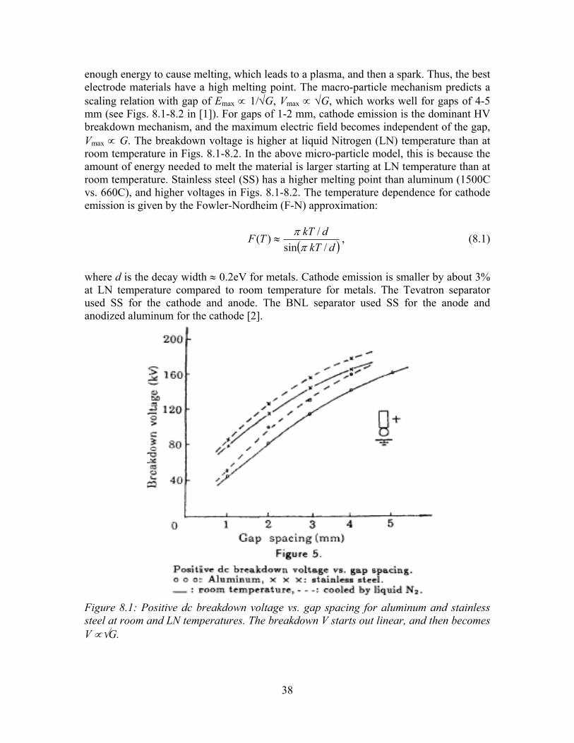
38

enough energy to cause melting, which leads to a plasma, and then a spark. Thus, the best electrode materials have a high melting point. The macro-particle mechanism predicts a scaling relation with gap of Emax 1/G, Vmax G, which works well for gaps of 4-5 mm (see Figs. 8.1-8.2 in [1]). For gaps of 1-2 mm, cathode emission is the dominant HV breakdown mechanism, and the maximum electric field becomes independent of the gap, Vmax G. The breakdown voltage is higher at liquid Nitrogen (LN) temperature than at room temperature in Figs. 8.1-8.2. In the above micro-particle model, this is because the amount of energy needed to melt the material is larger starting at LN temperature than at room temperature. Stainless steel (SS) has a higher melting point than aluminum (1500C vs. 660C), and higher voltages in Figs. 8.1-8.2. The temperature dependence for cathode emission is given by the Fowler-Nordheim (F-N) approximation:

dkT

dkTTF

/sin

/)(

, (8.1)

where d is the decay width 0.2eV for metals. Cathode emission is smaller by about 3% at LN temperature compared to room temperature for metals. The Tevatron separator used SS for the cathode and anode. The BNL separator used SS for the anode and anodized aluminum for the cathode [2].

Figure 8.1: Positive dc breakdown voltage vs. gap spacing for aluminum and stainless steel at room and LN temperatures. The breakdown V starts out linear, and then becomes V G.

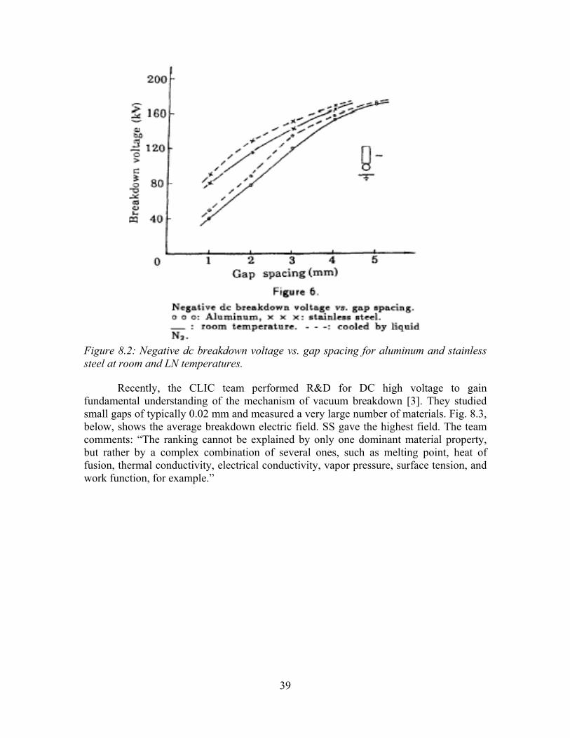
39

Figure 8.2: Negative dc breakdown voltage vs. gap spacing for aluminum and stainless steel at room and LN temperatures.

Recently, the CLIC team performed R&D for DC high voltage to gain fundamental understanding of the mechanism of vacuum breakdown [3]. They studied small gaps of typically 0.02 mm and measured a very large number of materials. Fig. 8.3, below, shows the average breakdown electric field. SS gave the highest field. The team comments: “The ranking cannot be explained by only one dominant material property, but rather by a complex combination of several ones, such as melting point, heat of fusion, thermal conductivity, electrical conductivity, vapor pressure, surface tension, and work function, for example.”

40

Figure 8.3: Average breakdown field from [3].

An excellent KEK-Riken study [4] of cathode current vs. E for different gap distances used an effective cathode area of 1cm2 and gaps in the range 0.3 – 1.25mm and gave fit parameters and plots for 1nA cathode current. The study found that Ti is better than SS (see Fig. 8.4). This contradicts the data in Fig. 8.3: Fig. 8.4 used NK SS, whereas Fig. 8.3 used 316LN SS. Presumably, this explains the difference.

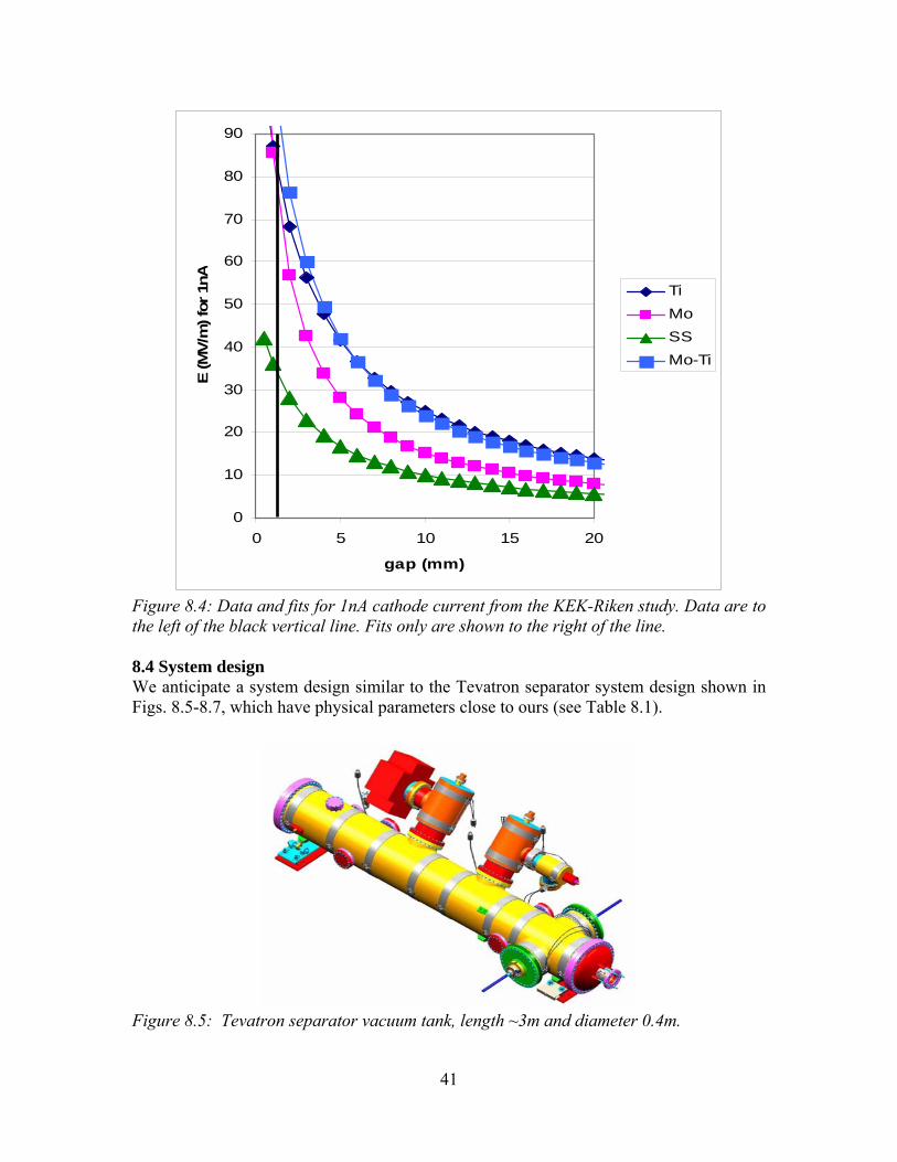
41

0

10

20

30

40

50

60

70

80

90

0 5 10 15 20

gap (mm)

E (M

V/m

) fo

r 1n

A

Ti

Mo

SS

Mo-Ti

Figure 8.4: Data and fits for 1nA cathode current from the KEK-Riken study. Data are to the left of the black vertical line. Fits only are shown to the right of the line. 8.4 System design We anticipate a system design similar to the Tevatron separator system design shown in Figs. 8.5-8.7, which have physical parameters close to ours (see Table 8.1).

Figure 8.5: Tevatron separator vacuum tank, length ~3m and diameter 0.4m.

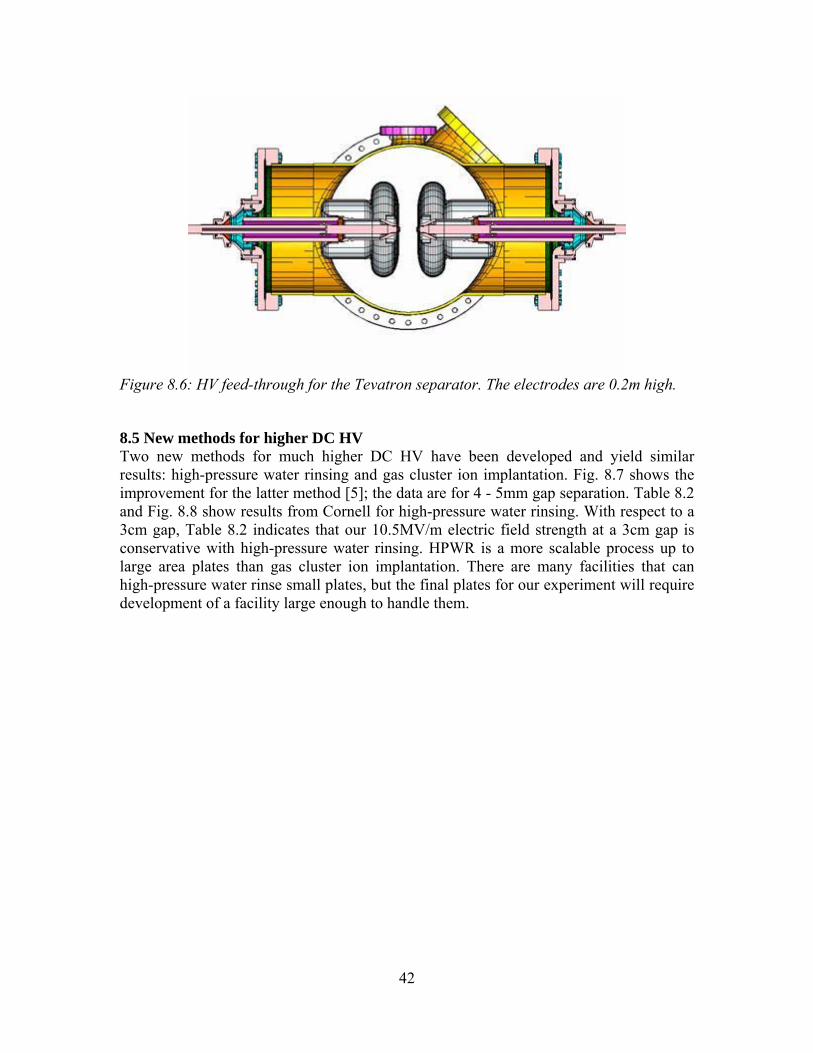
42

Figure 8.6: HV feed-through for the Tevatron separator. The electrodes are 0.2m high. 8.5 New methods for higher DC HV Two new methods for much higher DC HV have been developed and yield similar results: high-pressure water rinsing and gas cluster ion implantation. Fig. 8.7 shows the improvement for the latter method [5]; the data are for 4 - 5mm gap separation. Table 8.2 and Fig. 8.8 show results from Cornell for high-pressure water rinsing. With respect to a 3cm gap, Table 8.2 indicates that our 10.5MV/m electric field strength at a 3cm gap is conservative with high-pressure water rinsing. HPWR is a more scalable process up to large area plates than gas cluster ion implantation. There are many facilities that can high-pressure water rinse small plates, but the final plates for our experiment will require development of a facility large enough to handle them.

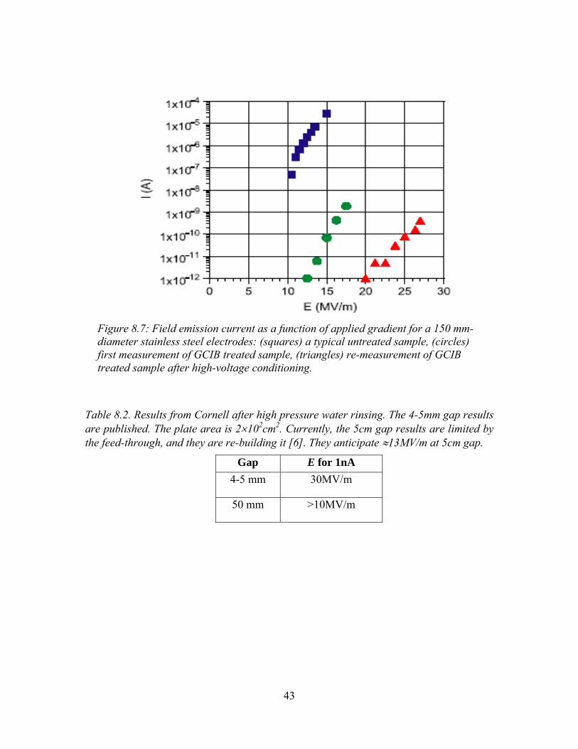
43

Table 8.2. Results from Cornell after high pressure water rinsing. The 4-5mm gap results are published. The plate area is 2102cm2. Currently, the 5cm gap results are limited by the feed-through, and they are re-building it [6]. They anticipate 13MV/m at 5cm gap.

Gap E for 1nA

4-5 mm 30MV/m

50 mm >10MV/m

Figure 8.7: Field emission current as a function of applied gradient for a 150 mm-diameter stainless steel electrodes: (squares) a typical untreated sample, (circles) first measurement of GCIB treated sample, (triangles) re-measurement of GCIB treated sample after high-voltage conditioning.

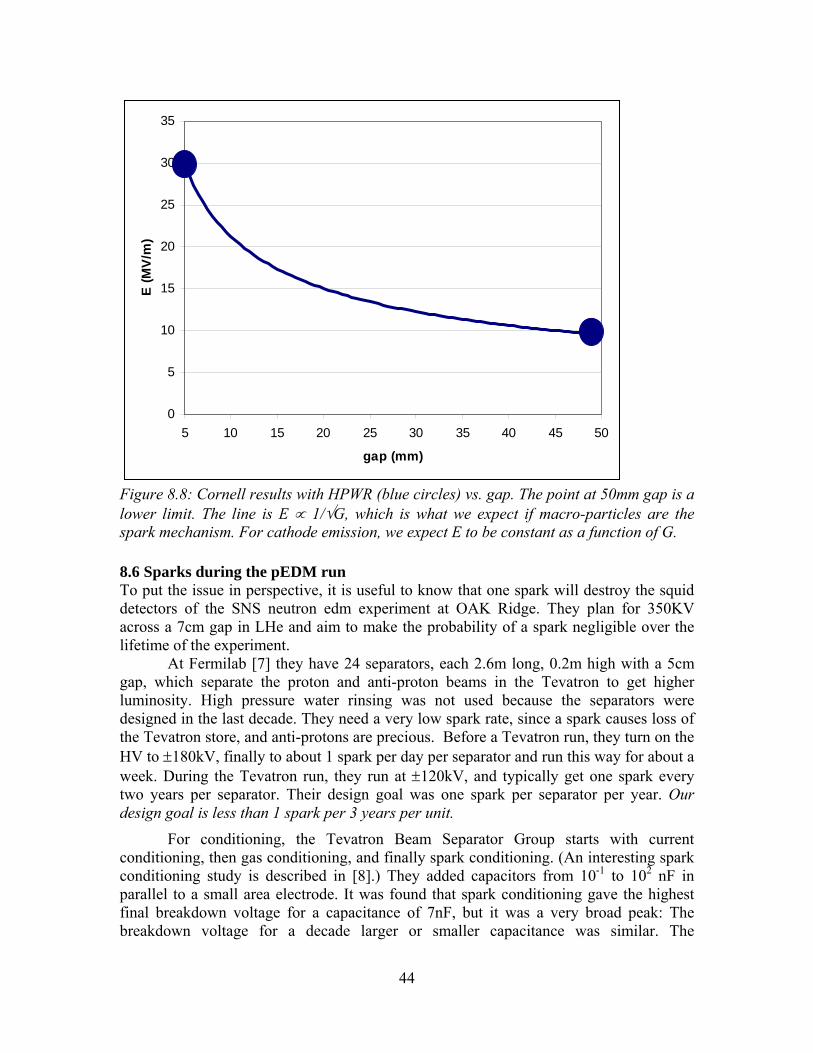
44

0

5

10

15

20

25

30

35

5 10 15 20 25 30 35 40 45 50

gap (mm)

E (

MV

/m)

Figure 8.8: Cornell results with HPWR (blue circles) vs. gap. The point at 50mm gap is a lower limit. The line is E 1/G, which is what we expect if macro-particles are the spark mechanism. For cathode emission, we expect E to be constant as a function of G. 8.6 Sparks during the pEDM run To put the issue in perspective, it is useful to know that one spark will destroy the squid detectors of the SNS neutron edm experiment at OAK Ridge. They plan for 350KV across a 7cm gap in LHe and aim to make the probability of a spark negligible over the lifetime of the experiment.

At Fermilab [7] they have 24 separators, each 2.6m long, 0.2m high with a 5cm gap, which separate the proton and anti-proton beams in the Tevatron to get higher luminosity. High pressure water rinsing was not used because the separators were designed in the last decade. They need a very low spark rate, since a spark causes loss of the Tevatron store, and anti-protons are precious. Before a Tevatron run, they turn on the HV to 180kV, finally to about 1 spark per day per separator and run this way for about a week. During the Tevatron run, they run at 120kV, and typically get one spark every two years per separator. Their design goal was one spark per separator per year. Our design goal is less than 1 spark per 3 years per unit.

For conditioning, the Tevatron Beam Separator Group starts with current conditioning, then gas conditioning, and finally spark conditioning. (An interesting spark conditioning study is described in [8].) They added capacitors from 10-1 to 102 nF in parallel to a small area electrode. It was found that spark conditioning gave the highest final breakdown voltage for a capacitance of 7nF, but it was a very broad peak: The breakdown voltage for a decade larger or smaller capacitance was similar. The

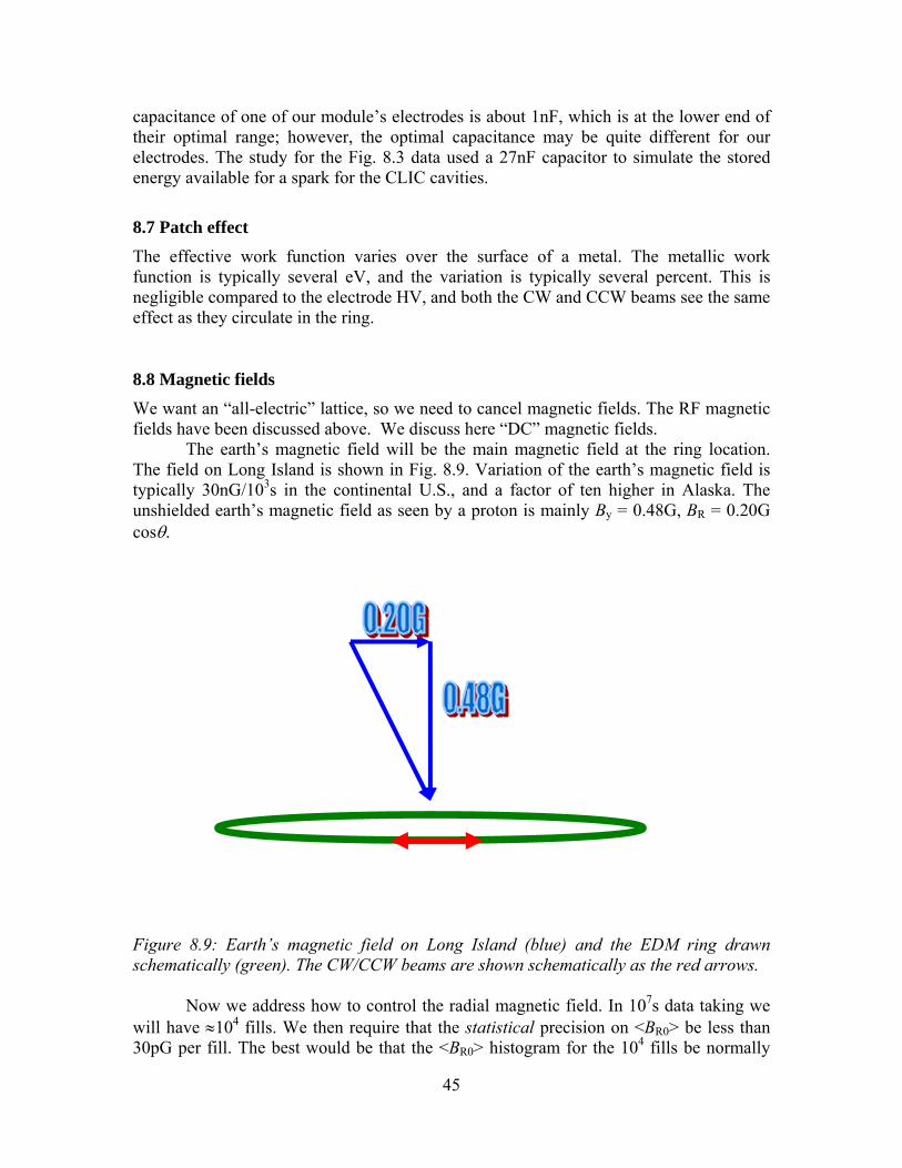
45

capacitance of one of our module’s electrodes is about 1nF, which is at the lower end of their optimal range; however, the optimal capacitance may be quite different for our electrodes. The study for the Fig. 8.3 data used a 27nF capacitor to simulate the stored energy available for a spark for the CLIC cavities.

8.7 Patch effect

The effective work function varies over the surface of a metal. The metallic work function is typically several eV, and the variation is typically several percent. This is negligible compared to the electrode HV, and both the CW and CCW beams see the same effect as they circulate in the ring.

8.8 Magnetic fields

We want an “all-electric” lattice, so we need to cancel magnetic fields. The RF magnetic fields have been discussed above. We discuss here “DC” magnetic fields.

The earth’s magnetic field will be the main magnetic field at the ring location. The field on Long Island is shown in Fig. 8.9. Variation of the earth’s magnetic field is typically 30nG/103s in the continental U.S., and a factor of ten higher in Alaska. The unshielded earth’s magnetic field as seen by a proton is mainly By = 0.48G, BR = 0.20G cos.

Figure 8.9: Earth’s magnetic field on Long Island (blue) and the EDM ring drawn schematically (green). The CW/CCW beams are shown schematically as the red arrows.

Now we address how to control the radial magnetic field. In 107s data taking we will have 104 fills. We then require that the statistical precision on <BR0> be less than 30pG per fill. The best would be that the <BR0> histogram for the 104 fills be normally

46

distributed about zero, with sigma less than 30pG. If this is not the case, then we must fit the data, as shown schematically in Fig. 8.10. The slope is known, but we will verify this from the fit. The intercept gives the EDM. The crucial point is that the measurement of zero average radial magnetic field be truly zero, without a systematic offset of more than 0.3pG. (Systematics are discussed in Section 9.)

Thus, we need a system to reduce BR0 <30pG per fill. We start effectively at 8mG, from the effect of the earth’s magnetic field BR1 on the BPM measurements of the CW/CCW vertical closed orbit difference, which varies around the ring as cos. The BPMs around the ring will see this azimuthal dependence, and therefore 8mG is very conservative. We then need a factor of 3108 reduction. We plan that the beam vacuum chamber of diameter 0.4m will have passive magnetic shielding. There will be coils outside to reduce the field entering the vacuum chamber, and coils inside the vacuum chamber. If each has a modest factor of 103, for example, then the total factor will be 109-more than is needed. These plans need to be value engineered (assessment of the cost of passive vs. active shielding, and so on). For more information, see Appendix 5.

Figure 8.10: Schematic representation of a fit to dSy/dt = e(g-2)hBR0/m + dE. The blue curve has a zero EDM. The green curve has a non-zero EDM. The red arrow represents the dE term.

47

8.9 Electric field R&D: constructing the first E module

The engineering design will start out with the Tevatron separator engineering design and iterate from there.2

Table 8.3. Cost estimate for first E module. Estimate by Sumanta Nayak, C-AD engineer.

Name Dimension (mm) Design/ Plan Hrs M/L

Man /Ass Hrs Cost ($)

Cont (%)

Final Cost

Electrode Plate 2400 X 200 x 20 35 SS304 70 22037 25 27546

Vacuum Tank 460 dia X 2600 Lth X 20 Thk 80 SS304 200 28594 25 35742

Vacuum Tank End Flange

460 dia X 20 thk plate 15 SS304 30 10810 25 13513

Ports Assume 8" (200)

size 10 SS304 18 28362 25 35453

The Vacuum Tank assemble 50 5000 25 6250

Frame assembling & with Plate 30 3000 25 3750

Inner Structure Support System 75 100 27500 75 48125

Gauges 15000 50 22500

Vacuum Equipment

500 l/s Ion Pumps with controller 18000 10 19800

Turbo Pump 20000 15 23000

Bake out card 20000 15 23000

Blankets 35000 15 40250

Vac Equip hook up 40 4000 25 5000Instrumentation and

Testing 100 35000 50 52500

Total 272313 356438

2 Oleg Prokofiev, the Tevatron separator team leader, said “one pair of the Tevatron SS electrodes cost $15K in FY00$, and the module construction and tests would require a couple hundred thousand FY09$”. This is a good sanity check of our estimate.

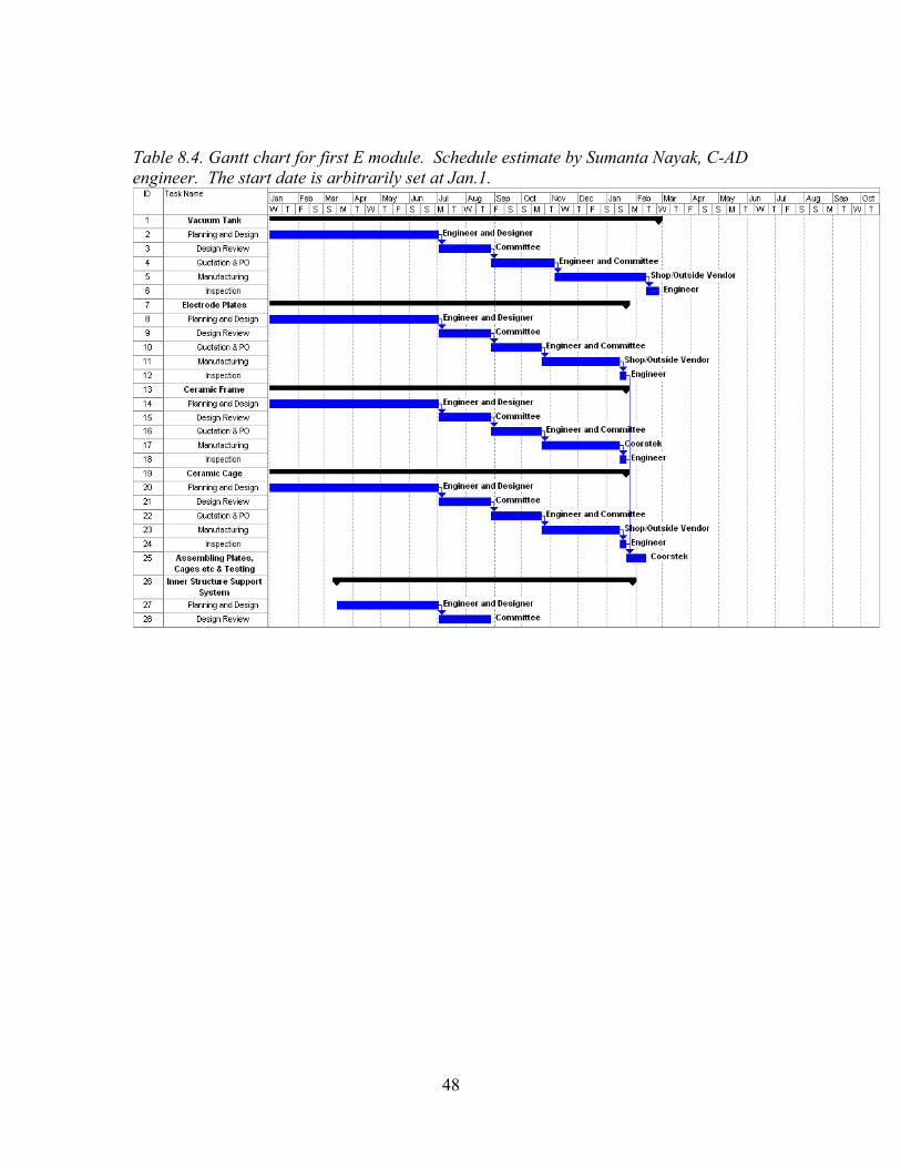
48

Table 8.4. Gantt chart for first E module. Schedule estimate by Sumanta Nayak, C-AD engineer. The start date is arbitrarily set at Jan.1.

49

References

1. H. Fengnian and W. Weihan, IEEE Transactions on Electrical Insulation 25, 557 (1990).

2. P. Pile et al., Nucl. Instrum. Meth. A321, 48 (1992). 3. A. Descoeudres et al., Phys. Rev. STAB 12, 032001 and 092001 (20009). 4. F. Furuta et al., Nucl. Instrum. Meth. A538, 33 (2005). 5. D. Swenson et al., Nucl. Instrum. Meth. B261, 630 (2007). 6. K. Smolenski, Cornell University, private communication. 7. Fermilab information from O. Prokofiev, Tevatron Beam Separator Group,

private communication. 8. G.A. Farrall, IEEE Trans. on Elect. Insulation 20(5), 815 (1985).

50

9. RELATIVE BEAM POSITION MONITORS 9.1 Measuring Br0

This experiment will search for proton spin precession out of the horizontal plane (where it is initially parallel or anti-parallel to the momentum vector) into the vertical, as a result of a large radial electric field acting on the proton's EDM. Given the parameters of this experiment, an EDM of dp=10-29 ecm would lead to a precession rate into the vertical of 3 nrad/s. However, this precession could also be caused by a net radial magnetic field Br0 around the storage ring of 0.15 pG acting on the proton's magnetic moment. Careful attention to magnetic shielding will allow sensitive magnetometers to measure Br0 to the required accuracy, allowing the EDM effect to be separated from radial magnetic field effects.

The measurement of Br0 will rely on the fact that the Lorentz force from Br0 ˆ r will split the CW and CCW beams in the vertical direction. In the absence of such splitting, and if the currents were identical, the counter-circulating beams would not produce a DC magnetic field. With a non-zero vertical splitting, a DC magnetic field Bs is produced in the horizontal plane. The magnitude of Bs is proportional to the beam current and the splitting. The splitting, in turn, is proportional to Br0 and inversely proportional to the vertical tune squared, Qy

2 . Modulating Qy at ωm will introduce an AC component into the

splitting and Bs. SQUID magnetometers and lock-in techniques will measure the component of Bs at the modulation frequency ωm, and extract Br0. This value of Br0 will reflect the quantity of interest: the spatial average of the radial magnetic field over the storage volume weighted by the beam distributions.

In the case of uniform vertical focusing, the field to be detected from the beam splitting 2δy is given by:

Bs r, 0, ,m 0

42I

r2 y 4Acos mt ˆ x , where y cR0Br0

ErQy2 1.0 pm

= 0.4 103 fT.

(9.1)

(See Appendix 6 for further details.) Given a measurement time of 107 seconds and modulation amplitude A=0.1, the EDM experiment requires a magnetometer system with an overall sensitivity of 1.25 fT/√Hz at the modulation frequency ωm, assuming a 1 Hz bandwidth. 9.2 Sensitive magnetometry using SQUIDS Magnetometers with the required sensitivity are available. They use at least two different techniques. Atomic magnetometers, such as the potassium magnetometer operating in the spin exchange relaxation free (SERF) regime, developed by M. Romalis' group at Princeton, have demonstrated sensitivities of <1 fT/√Hz for B fields with ωm > 35 Hz [1, 2]. Such systems may become available commercially in the next year or two [3]. A second approach, which we propose for use in the pEDM experiment, would make use of commercially available, low temperature DC superconducting quantum interference

51

devices (LTS dc SQUIDs). These have demonstrated sensitivities of 1 fT/√Hz [4], and bandwidths in flux-locked loop operation of several kHz (thus allowing ωm up to 1 kHz or so). Laboratory devices have achieved even better performance of 0.7 fT/√Hz [5]. In principle, a single pickup coil and SQUID sensor with these systems could meet the minimum requirements of the EDM experiment. In practice, many pickup coils would be placed on either side of the beams, with their normals in the horizontal in order to detect Bs (see Fig. 9.1). (Excessive ambient magnetic field noise can be mitigated by using gradient pick-up coils to preserve the signal but cancel background.) Using approximately 100 such systems, in 10 to 20 locations around the storage ring, will allow a robust measurement of Br0 with a S/N >> 5.

Figure 9.1: Schematic of a possible SQUID BPM station. The beams are in the innermost G10 beam pipe, which also includes a very thin-grounded conductor to attenuate high (MHz) frequency fields. The horizontal Bs field is picked up by the sense coils, which are attached by shielded superconducting wire (not shown) to the SQUIDs (which are also shielded). The system is carefully shielded with a low-noise ferrite shield and several layers of μ-metal.

These fT/√Hz sensitivities are only attained with strict attention to both magnetic shielding and to reducing magnetic field noise. The beam position monitor (BPM) stations will supplement the storage ring shielding with additional layers of μ-metal. A MnZn ferrite shield with low magnetic field noise will be used in the innermost layer to reduce the ambient field noise at ωm below a fT/√Hz [2, 6]. Magnetic field noise from RF sources and from the bunched beams themselves will be attenuated by a very thin, grounded conductor between the beams and the pick-up coils [7, 8]. The conductor will

52

pass the components of Bs at ωm, but severely attenuate the components at the much higher bunch frequencies.

The BPMs will measure the field at a finite number of locations, m. Fits to the BPM data will yield Br0 and estimates of a few higher-order multipoles BrN in the radial field distribution, where N ≤ m/2. Multipoles beyond N=0 average out around the storage ring and do not mimic an EDM. However, they can influence the average BPM reading and extraction of Br0 (though their weight drops rapidly as Qy

2 /N 2). Higher-order terms

beyond m/2 will be measured using custom or commercial atomic magnetometers [3] by mapping the radial field around the ring, including between the ring electrodes. Correction coils will be used to minimize these terms.

Other tools are available to ensure that the limits on the measurement of Br0 are met. Beam cooling (e.g., stochastic) could lead to a smaller vertical tune Qy, enhancing the Br0-induced beam splitting and increasing the BPM signal/noise. Also, varying the relative strengths of the quads used for vertical focusing may yield additional information on the radial B field distribution, making the extraction of Br0 more robust. 9.3 Earth’s magnetic field shielding In order for this method to work, we need to shield the magnetic field in the ring from the earth’s field as well as noise due to various human activities (see Section 8 on E- and B-fields). As mentioned above, the magnetic field noise in the ring needs to be reduced to less than 0.15pG when averaged around the ring. Since we expect to have ~104 injections (stores), the B-field noise for the duration of a storage time can be up to 102 times that value, i.e., 15 pG on average per storage time. The radial component of the earth’s magnetic field integrated around the ring is expected to be zero. We will assume it to be 10 mG, and to achieve the needed attenuation we need a shielding factor of ~109. We plan to obtain the needed reduction factor of 109 using three approaches:

1) Feedback outside the ring (using Helmholtz coils in the ring tunnel). 2) Passive shielding (we expect a shielding factor of 104 to 105 using three to four

mu-metal layers). 3) Feedback inside the beam tube (using Helmholtz coils).

The relative beam position monitors need to achieve a much lower B-field noise level than the ring itself: 4 fG, vs. 0.15 pG, i.e., about 40 times smaller. However, this needs to be achieved at a frequency of 1-10 kHz (which is much easier, as shown in Fig. 9.2, below), and can be done by a combination of mu-metal shielding and a (~1cm) thick aluminum tube [9]. 9.4 Time dependent magnetic field shielding The magnetic field noise measured in a city environment [9] is of the order of several nT/√Hz in the frequency range of 0.1 to 1 Hz. The average value of this noise around the ring is expected to be just a tiny fraction of that level. However, here we will

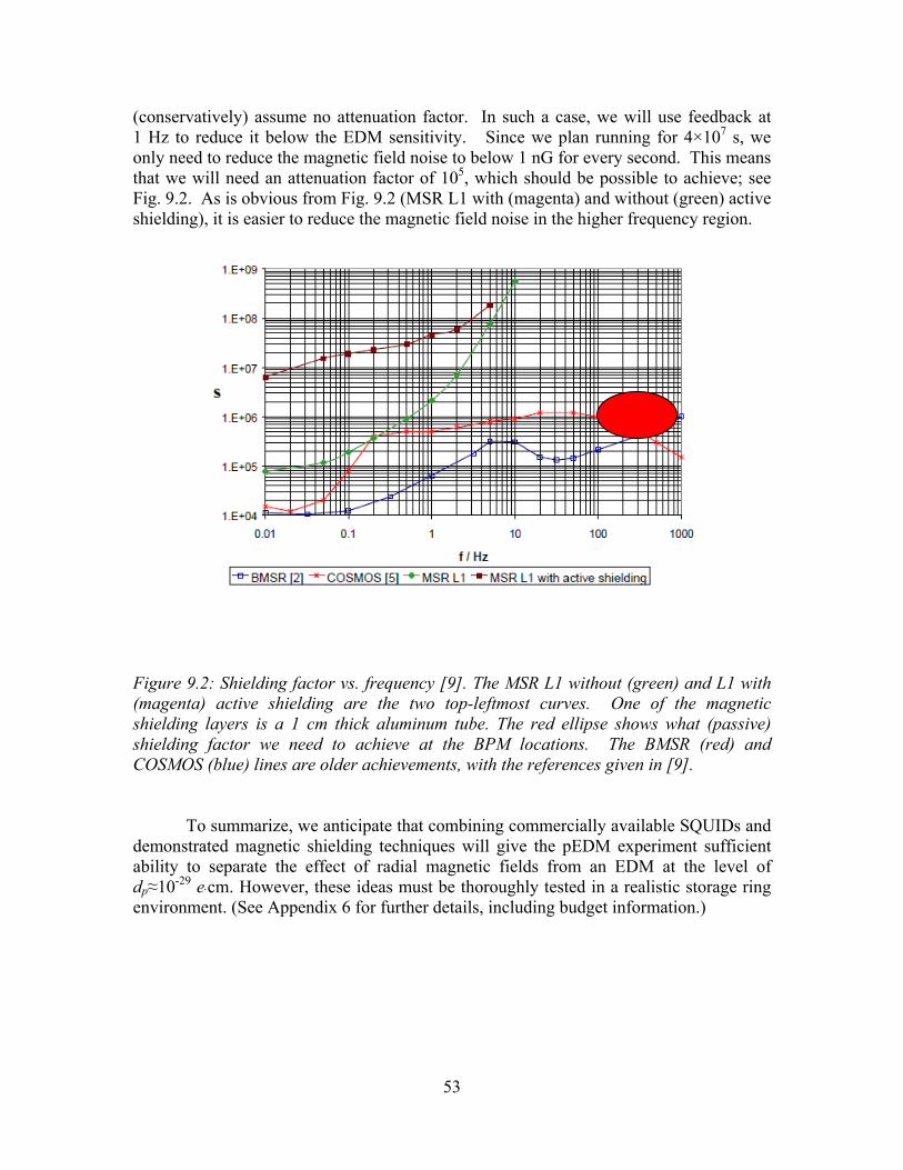
53

(conservatively) assume no attenuation factor. In such a case, we will use feedback at 1 Hz to reduce it below the EDM sensitivity. Since we plan running for 4×107 s, we only need to reduce the magnetic field noise to below 1 nG for every second. This means that we will need an attenuation factor of 105, which should be possible to achieve; see Fig. 9.2. As is obvious from Fig. 9.2 (MSR L1 with (magenta) and without (green) active shielding), it is easier to reduce the magnetic field noise in the higher frequency region.

Figure 9.2: Shielding factor vs. frequency [9]. The MSR L1 without (green) and L1 with (magenta) active shielding are the two top-leftmost curves. One of the magnetic shielding layers is a 1 cm thick aluminum tube. The red ellipse shows what (passive) shielding factor we need to achieve at the BPM locations. The BMSR (red) and COSMOS (blue) lines are older achievements, with the references given in [9].

To summarize, we anticipate that combining commercially available SQUIDs and demonstrated magnetic shielding techniques will give the pEDM experiment sufficient ability to separate the effect of radial magnetic fields from an EDM at the level of dp≈10-29 ecm. However, these ideas must be thoroughly tested in a realistic storage ring environment. (See Appendix 6 for further details, including budget information.)

54

References

1. J.C. Allred, R.N. Lyman, T.W. Kornack, and M.V. Romalis, Phys. Rev. Lett. 89, 130801 (2002).

2. T.W. Kornack, S.J. Smullin, S.-K. Lee, and M.V. Romalis, Appl. Phys. Lett. 90, 223501 (2007).

3. http://www.twinleaf.com 4. Tristan Technologies Model LSQ/20 LTS dc SQUID; Tristan Technologies, LLC,

San Deigo, CA 92121; http://www.tristantech.com 5. W. Vodel and K. Mäkiniemi, Meas. Sci. Technol. 3, 1155 (1992). 6. S.-K. Lee and M.V. Romalis, J. Appl. Phys. 103, 084904 (2008). 7. R. Gluckstern and B. Zotter, Phys. Rev. ST Accel. Beams 4, 024402 (2001). 8. A.M. Al-Khateeb et al., Phys. Rev. ST Accel. Beams 10, 064401 (2007). 9. Berlin Magnetically Shielded Room, available from:

http://www.ptb.de/cms/fileadmin/internet/fachabteilungen/abteilung_8/8.2_biosignale/8.21/mssr.pdf J. Bork, H.D. Hahlbohm, R. Klein, A. Schnabel, The 8-layered magnetically shielded room of the PTB: Design and construction, in Biomag2000, Proc. 12th Int. Conf. on Biomagnetism, J. Nenonen, R.J. Ilmoniemi, and T. Katila, eds. (Helsinki Univ. of Technology, Espoo, Finland, 2001), pp. 970-973.

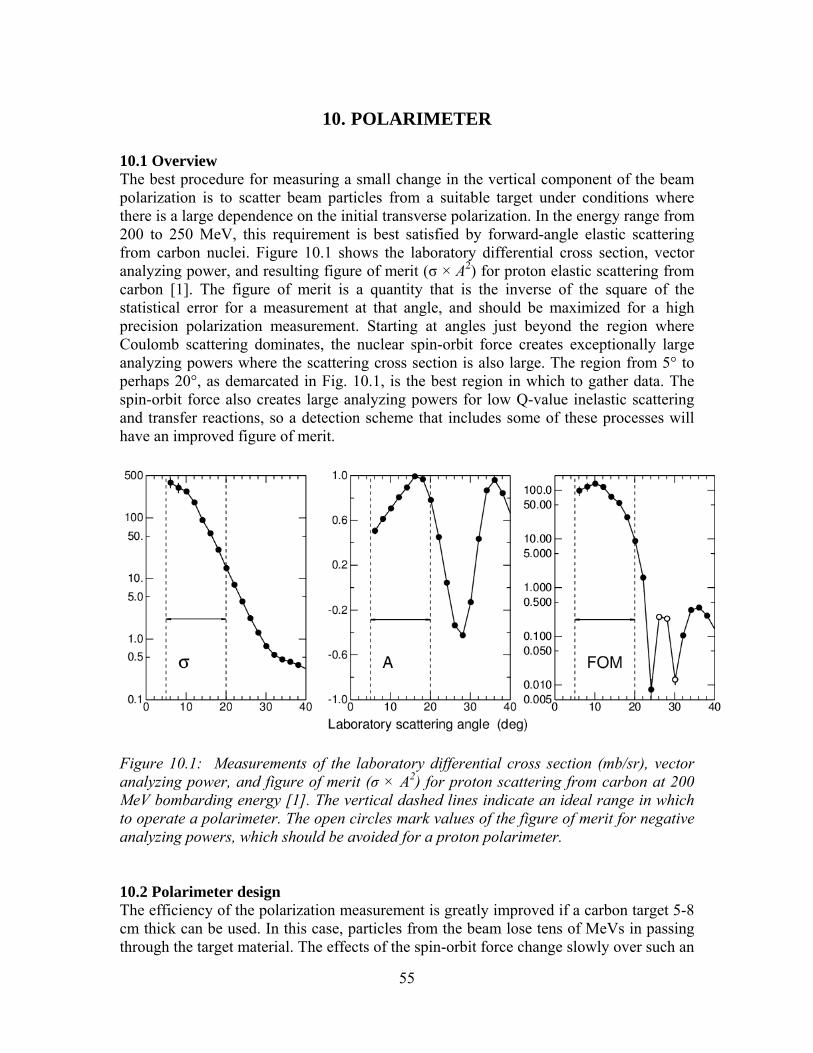
55

10. POLARIMETER

10.1 Overview The best procedure for measuring a small change in the vertical component of the beam polarization is to scatter beam particles from a suitable target under conditions where there is a large dependence on the initial transverse polarization. In the energy range from 200 to 250 MeV, this requirement is best satisfied by forward-angle elastic scattering from carbon nuclei. Figure 10.1 shows the laboratory differential cross section, vector analyzing power, and resulting figure of merit (σ × A2) for proton elastic scattering from carbon [1]. The figure of merit is a quantity that is the inverse of the square of the statistical error for a measurement at that angle, and should be maximized for a high precision polarization measurement. Starting at angles just beyond the region where Coulomb scattering dominates, the nuclear spin-orbit force creates exceptionally large analyzing powers where the scattering cross section is also large. The region from 5° to perhaps 20°, as demarcated in Fig. 10.1, is the best region in which to gather data. The spin-orbit force also creates large analyzing powers for low Q-value inelastic scattering and transfer reactions, so a detection scheme that includes some of these processes will have an improved figure of merit.

Figure 10.1: Measurements of the laboratory differential cross section (mb/sr), vector analyzing power, and figure of merit (σ × A2) for proton scattering from carbon at 200 MeV bombarding energy [1]. The vertical dashed lines indicate an ideal range in which to operate a polarimeter. The open circles mark values of the figure of merit for negative analyzing powers, which should be avoided for a proton polarimeter. 10.2 Polarimeter design The efficiency of the polarization measurement is greatly improved if a carbon target 5-8 cm thick can be used. In this case, particles from the beam lose tens of MeVs in passing through the target material. The effects of the spin-orbit force change slowly over such an

56

energy range. Efficiencies above 1% have been obtained [2] with thick targets in double-scattering spectrometers. One goal of polarimeter feasibility experiments is to demonstrate that such high efficiencies are possible in a storage ring environment where a thick target would be positioned at the edge of the beam and intercept relatively few particles on each passage of the beam. Another goal is to demonstrate that it is possible to correct for systematic errors arising from beam rate and misalignment effects in a storage ring where the beam intensity and other properties are changing with time. When work on these two polarimeter goals began in earnest in 2007, the plan was to build a deuteron storage ring EDM experiment at Brookhaven National Laboratory. A proposal was written to begin work with the polarized deuteron beam in the Cooler Synchrotron (COSY) located at Jülich, Germany. The laboratory differential cross section, analyzing power, and figure of merit for deuteron scattering from carbon [3], as shown in Fig. 10.2, are strikingly similar to those for protons, and a similar angle range from 5° to 20° is optimal for polarization measurements. Efficient polarimeters have been constructed for deuterons as well as protons [4,5]. So even when the Brookhaven effort was redirected toward protons, work continued with the deuteron setup at COSY because the similarity of these two cases meant that any results for one would apply equally well to the other.

Figure 10.2: Measurements of the laboratory differential cross section (mb/sr), the vector analyzing power iT11, and the figure of merit (dσ/dΩ × (iT11)

2) for deuteron elastic scattering from carbon at 270 MeV [1]. 10.3 A possible EDM polarimeter Figure 10.3 shows an expanded view of one side of a polarimeter, with the locations of the major components noted. The electrostatic lens is the first element of an electrostatic bending region. The scale is in centimeters. The polarimeter needs to end about 1 m from the target. The target comes in from either above or below in order to preserve left-right symmetry, and is a block of carbon about 6 cm in length. The block is positioned on the edge of the beam. Either steering or electrically-driven white noise is applied to the beam, causing it to move slowly onto the leading face of the target. This arrangement is symmetric from the front or rear; it allows a single target to serve as the source of

57

polarization information for beams circulating in either direction. Scattering of particles in the down and up directions provides information on the horizontal plane polarization component, so this scattering will be included in the data acquisition stream.

Detectors that observe scattered, charged particles emitted from thick targets are optimally located after some absorber has removed all but the elastic and low Q-value events. This removes the events with low polarization dependence and allows the detector and data acquisition system to be concentrated on events that produce a useful polarization signal. The detectors will be able to respond to charged-particle events with a minimum of dead time and small systematic errors. The types under consideration include multi-resistive plate chambers, micro-megas chambers, and gas electron multiplier chambers. The final choice will not be made until a prototype of each system has been tested with the beam at a storage ring facility. Segmentation of the sensitive volume into ~100 elements will be essential to reconstruct the scattering direction. Possible enhancements of the basic detector might include separated planes for time-of-flight discrimination or a leading time-projection chamber to provide directional event reconstruction.

Figure 10.3: A possible layout of one half of an EDM ring polarimeter with a thick carbon extraction target located on a motor drive, an expansion region for scattering between 5° and 20°, an absorber built into the vacuum walls, a final region for a detector, and the first electrostatic lens at the front of a bending region. The beam is denoted by a short-dashed line. Electric shielding plates and deflecting plates located at 1.5 cm from the beam are included. The dimensions are in centimeters. Scattered particles with transmit through the shielding plates. 10.4 Suppression of geometric and rate errors in real time An experiment to learn how to manage geometric and rate-induced systematic errors in the polarimeter was conducted successfully with the COoler SYnchrotron (COSY) at the

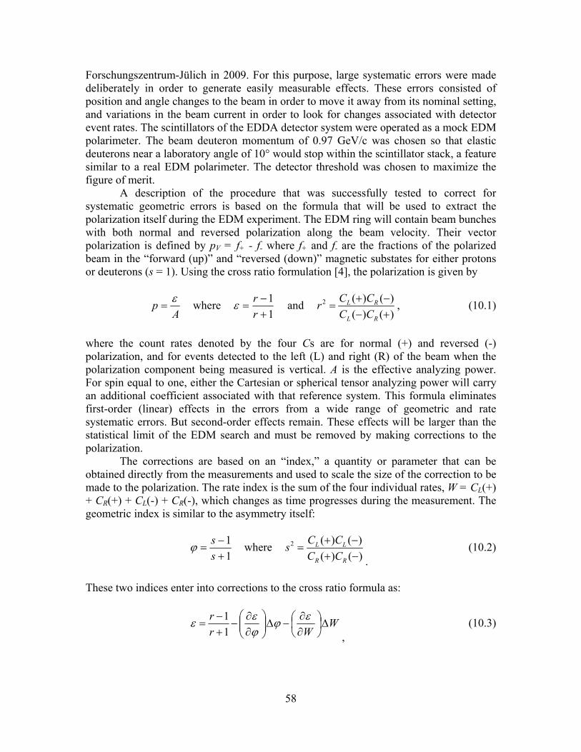
58

Forschungszentrum-Jülich in 2009. For this purpose, large systematic errors were made deliberately in order to generate easily measurable effects. These errors consisted of position and angle changes to the beam in order to move it away from its nominal setting, and variations in the beam current in order to look for changes associated with detector event rates. The scintillators of the EDDA detector system were operated as a mock EDM polarimeter. The beam deuteron momentum of 0.97 GeV/c was chosen so that elastic deuterons near a laboratory angle of 10° would stop within the scintillator stack, a feature similar to a real EDM polarimeter. The detector threshold was chosen to maximize the figure of merit. A description of the procedure that was successfully tested to correct for systematic geometric errors is based on the formula that will be used to extract the polarization itself during the EDM experiment. The EDM ring will contain beam bunches with both normal and reversed polarization along the beam velocity. Their vector polarization is defined by pV = f+ - f- where f+ and f- are the fractions of the polarized beam in the “forward (up)” and “reversed (down)” magnetic substates for either protons or deuterons (s = 1). Using the cross ratio formulation [4], the polarization is given by

Ap

where

1

1

r

r and 2 ( ) ( )

( ) ( )L R

L R

C Cr

C C

, (10.1)

where the count rates denoted by the four Cs are for normal (+) and reversed (-) polarization, and for events detected to the left (L) and right (R) of the beam when the polarization component being measured is vertical. A is the effective analyzing power. For spin equal to one, either the Cartesian or spherical tensor analyzing power will carry an additional coefficient associated with that reference system. This formula eliminates first-order (linear) effects in the errors from a wide range of geometric and rate systematic errors. But second-order effects remain. These effects will be larger than the statistical limit of the EDM search and must be removed by making corrections to the polarization. The corrections are based on an “index,” a quantity or parameter that can be obtained directly from the measurements and used to scale the size of the correction to be made to the polarization. The rate index is the sum of the four individual rates, W = CL(+) + CR(+) + CL(-) + CR(-), which changes as time progresses during the measurement. The geometric index is similar to the asymmetry itself:

1

1

s

s where 2 ( ) ( )

( ) ( )L L

R R

C Cs

C C

. (10.2)

These two indices enter into corrections to the cross ratio formula as:

WWr

r

1

1

, (10.3)

59

where the incremental differences, Δφ and ΔW, measure the departure of the index from its central value at the nominal beam setting and the derivatives (like the analyzing power) are properties of the polarimeter that are calibrated in advance. The experiment at COSY demonstrates several things. First, modifications from changes in event rates may be corrected separately from geometric effects. Second, a single index is sufficient in each case to parameterize the extent of a rate or geometry change so that a correction can be made. Third, changes in angle or position can be corrected using the same geometric index, a property likely to be best obeyed for forward-angle polarimeters. The rate and geometric indexes are composed of the same raw data that are used to calculate the polarization in Eq. (10.1) and are available in real time. As part of the analysis of the data from the COSY experiment, the derivatives for a variety of polarization observables besides the cross ratio polarization were constructed out of horizontal angle and position changes to ensure that their origin was understood. In part, the identification of a mechanism that produced each derivative helped to evaluate whether they would be subject to change over time after the calibration was completed. This model of the COSY experiment included: (1) vector and tensor polarizations for each polarized beam state, (2) analyzing powers for both vector and tensor polarization, (3) solid angle ratios, (4) the effective distance to the detector, which relates angle and position, (5) first and second derivatives of the cross section and two analyzing powers with respect to either an angle or position error, (6) effective rotation of the polarimeter in which horizontal asymmetries feed into vertical asymmetries, (7) coupling between vertical and horizontal changes for both angle and position, and (8) a low-momentum tail on the beam that passed the target and hit the right-side detector. The model reproduced the experimental data well, as measured by its reduced chi square value of 1.7--which is not one because some faulty beam stores were not removed from the data set. The ability of eq. (10.3) to correct measurements made in real time is illustrated in Fig. 10.4, which shows a test from the end of the COSY experiment. In this case, the polarization of the beam was in the vertical direction. (Once injected and stored, this component is expected to be stable for very long times, since it is parallel to the magnetic field in the bending magnets of the synchrotron ring.) The red points are the initial data for a simple left-right asymmetry, (CL - CR)/(CL + CR), where the systematic error effects are large and easy to see. There is a distortion from a flat distribution that rises to a peak at 6 s. This comes from a rate effect, since the extraction rate also peaks at that time. The rate correction by itself removes this and produces the blue points, to make a flatter distribution. But the asymmetry values are still wrong due to a geometric error that, when corrected, produces the black points. A straight line fit through these final points has a slope of (-4 ± 11) × 10-6 s-1, which is flat to within the errors of the original data. (In this example, the reduced error in the final data reflects the additional information from the opposite polarization state that was used to calculate the correction index φ.)

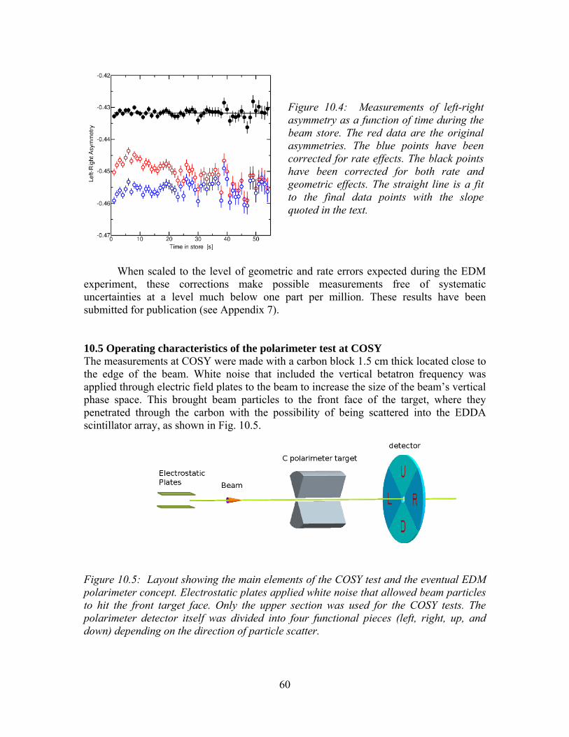
60

When scaled to the level of geometric and rate errors expected during the EDM experiment, these corrections make possible measurements free of systematic uncertainties at a level much below one part per million. These results have been submitted for publication (see Appendix 7). 10.5 Operating characteristics of the polarimeter test at COSY The measurements at COSY were made with a carbon block 1.5 cm thick located close to the edge of the beam. White noise that included the vertical betatron frequency was applied through electric field plates to the beam to increase the size of the beam’s vertical phase space. This brought beam particles to the front face of the target, where they penetrated through the carbon with the possibility of being scattered into the EDDA scintillator array, as shown in Fig. 10.5. Figure 10.5: Layout showing the main elements of the COSY test and the eventual EDM polarimeter concept. Electrostatic plates applied white noise that allowed beam particles to hit the front target face. Only the upper section was used for the COSY tests. The polarimeter detector itself was divided into four functional pieces (left, right, up, and down) depending on the direction of particle scatter.

Figure 10.4: Measurements of left-right asymmetry as a function of time during the beam store. The red data are the original asymmetries. The blue points have been corrected for rate effects. The black points have been corrected for both rate and geometric effects. The straight line is a fit to the final data points with the slope quoted in the text.

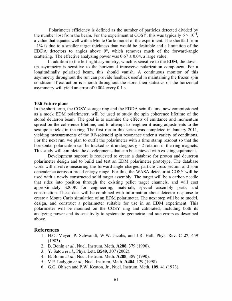
61

Polarimeter efficiency is defined as the number of particles detected divided by the number lost from the beam. For the experiment at COSY, this was typically 6 × 10-4, a value that equates well with a Monte Carlo model of the experiment. The shortfall from ~1% is due to a smaller target thickness than would be desirable and a limitation of the EDDA detectors to angles above 9°, which removes much of the forward-angle scattering. The effective analyzing power was 0.67 ± 0.04, a large value. In addition to the left-right asymmetry, which is sensitive to the EDM, the down-up asymmetry is sensitive to the horizontal transverse polarization component. For a longitudinally polarized beam, this should vanish. A continuous monitor of this asymmetry throughout the run can provide feedback useful in maintaining the frozen spin condition. If extraction is smooth throughout the store, then statistics on the horizontal asymmetry will yield an error of 0.004 every 0.1 s. 10.6 Future plans In the short term, the COSY storage ring and the EDDA scintillators, now commissioned as a mock EDM polarimeter, will be used to study the spin coherence lifetime of the stored deuteron beam. The goal is to examine the effects of emittance and momentum spread on the coherence lifetime, and to attempt to lengthen it using adjustments to the sextupole fields in the ring. The first run in this series was completed in January 2011, yielding measurements of the RF-solenoid spin resonance under a variety of conditions. For the next run, we plan to outfit the polarimeter with a time stamp readout so that the horizontal polarization can be tracked as it undergoes g - 2 rotation in the ring magnets. This study will complete the developments that can be achieved with existing equipment. Development support is requested to create a database for proton and deuteron polarimeter design and to build and test an EDM polarimeter prototype. The database work will involve measuring the forward-angle charged particle cross section and spin dependence across a broad energy range. For this, the WASA detector at COSY will be used with a newly constructed solid target assembly. The target will be a carbon needle that rides into position through the existing pellet target channels, and will cost approximately $200K for engineering, materials, special assembly parts, and construction. These data will be combined with information about detector response to create a Monte Carlo simulation of an EDM polarimeter. The next step will be to model, design, and construct a polarimeter suitable for use in an EDM experiment. This polarimeter will be mounted on the COSY ring and calibrated, including both its analyzing power and its sensitivity to systematic geometric and rate errors as described above. References

1. H.O. Meyer, P. Schwandt, W.W. Jacobs, and J.R. Hall, Phys. Rev. C 27, 459 (1983).

2. B. Bonin et al., Nucl. Instrum. Meth. A288, 379 (1990). 3. Y. Satou et al., Phys. Lett. B549, 307 (2002). 4. B. Bonin et al., Nucl. Instrum. Meth. A288, 389 (1990). 5. V.P. Ladygin et al., Nucl. Instrum. Meth. A404, 129 (1998). 6. G.G. Ohlsen and P.W. Keaton, Jr., Nucl. Instrum. Meth. 109, 41 (1973).

62

11. STATISTICAL SENSITIVITY AND SYSTEMATIC ERRORS OF THE EXPERIMENTAL METHOD

11.1 Expected signal of the pEDM experiment

The expected EDM signal, assuming the spin is along the momentum, is estimated by

0

1 2

22

,

ds d dEd E dE

dt dtdE

t t

(11.1)

where d, E are assumed to be orthogonal to each other. For E=10.5 MV/m, 95% E-field coverage of the ring, and an EDM of d=10-29 ecm, the rate of change in the vertical spin component is

31 8

0 0

0

2 2 10 e m 10.5MV/m 0.95 3 10 m/s

197 MeV fmnrad

3 .s

dEct t t

c

t t

(11.2)

We can make the following observations from equations (11.1) and (11.2):

1) The vertical component of the proton spin grows linearly with time to the extent that the beam polarization is constant. This growth, however, will in practice be limited by the spin coherence time (SCT) of the stored proton beam.

2) Equation (11.1) implies that the EDM effect is proportional to the E-field applied on the proton EDM.

3) Protons will be stored for 103 s, yielding about 3 rad of early-to-late change in their vertical spin component.

4) Lastly, a high efficiency polarimeter with high analyzing power that can detect the beam polarization as a function of time is essential to the success of the experiment. Using existing experimental data, we have estimated an average efficiency of 1.1% summing over the 2π azimuthal angle and an average analyzing power of 0.6 (i.e., 60%) for 0.7 GeV/c protons scattered off a solid carbon target.

Therefore, the maximum expected early-to-late normalized change in counting asymmetry related to EDM is of the order of 2 ppm. 11.2 Statistical error The statistical error, which has been estimated both analytically and confirmed numerically with a M.C. simulation, is given by

63

tot,c tot

2d p

pPAE N fT

, (11.3)

which holds for an extraction that keeps the same number of detected particles as a function of time. Assuming the parameters P = 0.8, A = 0.6, E = 10.5 MV/m, Ntot,c = 4×1010 particles/storage, an effective detection efficiency of f = 0.011/2, total running time Ttot = 107 s/year, and SCT of p = 103 s, we get a statistical error of ~1.8×10-29 ecm per year. The total polarimeter efficiency is estimated by a M.C. to be 1.1% for both the left/right and up/down counts. Using only the left/right counts for the EDM estimation, we get the factor of two reduction used above. The M.C. showed the analyzing power of the polarimeter to be 60%. The same M.C. was used to estimate the efficiency and analyzing power of the EDDA detector in the polarimeter systematic error studies at COSY, and its predictions were confirmed.

A numerical study of the statistical sensitivity is shown in Figs. 11.1, and 11.2, below. The vertical component due to an EDM was made to grow at a rate of 13.5 nrad/s, corresponding to 4.5×10-29 ecm. P0=0.8; A=0.6; f=0.55%; the number of stored particles per injection used were only 2×1010; and the total experiment running time was assumed constant to 4×107 s (defined as four calendar years). Hence, the total number of counts used for the EDM were 2×1012. The polarization lifetime was assumed to be 103s and following the functional form:

20 1P P B t , (11.4)

where B is such that at t=103s the beam polarization drops to 0.5 of its original value. The polarization model represented by eq. (11.4) is only approximately right at times up to 2000 s; it breaks down at much longer times. However, for this study it was deemed to be good enough. We have started studies with more realistic polarization models, indicating conclusions similar to those presented below.

64

Figure 11.1: (L-R)/(L+R) vs. time [s], is as well as the fit results to two parameters (slope and dc offset). The total counts used are 4×1012, with P0=0.8, and A=0.6. The slope is estimated with 3.8 sigma statistical accuracy. The fit results confirm the result of eq. (11.3).

Following the suggestion of the technical review committee in 2009, we have also looked into modulating the data-taking rate as is done in other EDM and high precision experiments. One can optimize the statistics by taking most of the data at early and late times only. However, we need to have enough counts to monitor and control the forward spin direction during storage. We therefore decided to keep taking data even in between the early and late times, but at a much lower rate. We multiplied the counting rate by a factor of 4 for the first and last 100s of storage time and reduced the rate in between by the same factor, keeping the total counts the same. The result is shown in Fig. 11.2.

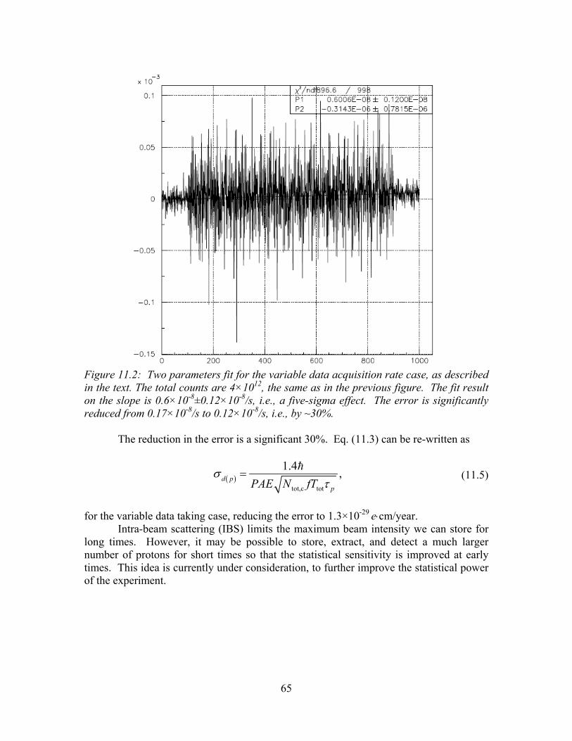
65

Figure 11.2: Two parameters fit for the variable data acquisition rate case, as described in the text. The total counts are 4×1012, the same as in the previous figure. The fit result on the slope is 0.6×10-8±0.12×10-8/s, i.e., a five-sigma effect. The error is significantly reduced from 0.17×10-8/s to 0.12×10-8/s, i.e., by ~30%.

The reduction in the error is a significant 30%. Eq. (11.3) can be re-written as

tot,c tot

1.4,d p

pPAE N fT

(11.5)

for the variable data taking case, reducing the error to 1.3×10-29 ecm/year.

Intra-beam scattering (IBS) limits the maximum beam intensity we can store for long times. However, it may be possible to store, extract, and detect a much larger number of protons for short times so that the statistical sensitivity is improved at early times. This idea is currently under consideration, to further improve the statistical power of the experiment.

66

11.3 Systematic errors of the pEDM experiment

As described earlier in this proposal, to probe the average radial B-field we plan to store beams in both clockwise (CW) and counter-clockwise (CCW) directions. A radial B-field will precess the proton spins of both beams, just as a radial E-field would in the presence of an EDM. However, only a radial B-field will split (separate) the two beams vertically3. This vertical separation depends on the strength of the vertical focusing system. To maximize the beam separation we plan to use weak vertical focusing (the tune will be 0.2 at injection and become 0.1 within the first ~50 s) while keeping the horizontal focusing greater than 1 to maximize the ring admittance. The consequences of a small vertical tune are: 1) maximized sensitivity to a background radial B-field, 2) maximized spin coherence time, and 3) reduced vertical ring admittance. We partially compensate for item three by increasing the vertical storage region to ±4 cm. We plan to modulate the vertical tune so that the beam separation is also modulated at the same frequency.

Table 11.1, below, briefly presents a list of systematic errors and how we plan to handle them. Each systematic error listed has been described in separate papers and many are discussed elsewhere in this proposal or in supplementary material. More information about them is available upon request. The discussion following the table is mostly limited to the radial B-field effect, because it is the strictest, and two errors not included in the table:

1) The presence of a net radial B-field could mimic an EDM signal, but will also split the beams vertically at the same time. The same is true for any vertical force that can cause splitting between the two beams, because it will be perceived as caused by a radial B-field. Gravitational forces, E-fields or any other type of fields applying the same force to the two counter-rotating beams are of no consequence.

2) Beam and/or spin dynamics resonances. We need to map out the resonances in the neighborhood of the operating n-values and we will reduce the field multipoles below the needed level. We do not expect this issue to be a major problem, but will study this effect using particle momentum and spin tracking software.

3) Wake fields due to the lattice structure. Preliminary estimations indicate they are manageable. However, we plan to continue the estimations with the help of software packages used by experts in the field (e.g., Micro-Wave Studio).

3 An AC electric field that is systematically different for the two beams would also move them apart. This can happen in the RF-cavity if there are substantial losses for the two beams around the ring and the cavity is vertically misaligned. It can also happen if there are significant vertical forces due to image charges at a place in the ring where the counter-rotating (CR) beams do not overlap in time and the CR beam intensities are not the same. We plan to use vertical plates wherever possible to eliminate the vertical forces due to image charges. More details are given later in this section.

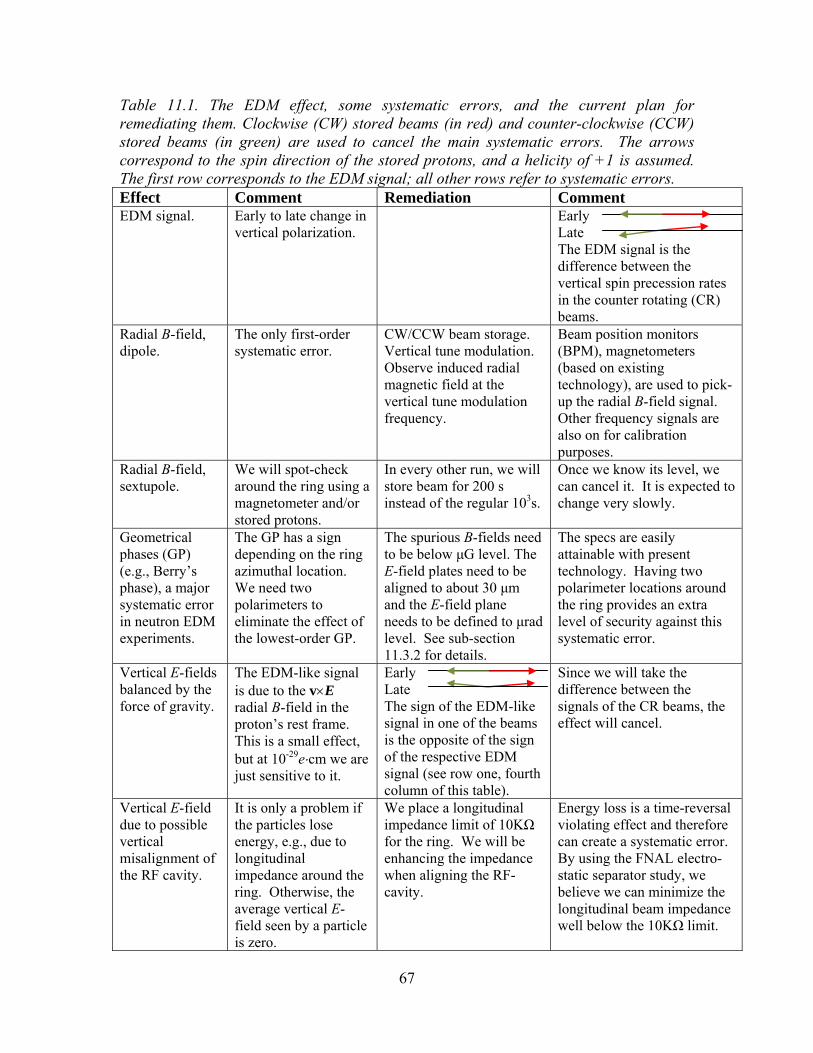
67

Table 11.1. The EDM effect, some systematic errors, and the current plan for remediating them. Clockwise (CW) stored beams (in red) and counter-clockwise (CCW) stored beams (in green) are used to cancel the main systematic errors. The arrows correspond to the spin direction of the stored protons, and a helicity of +1 is assumed. The first row corresponds to the EDM signal; all other rows refer to systematic errors. Effect Comment Remediation Comment EDM signal. Early to late change in

vertical polarization. Early

Late The EDM signal is the difference between the vertical spin precession rates in the counter rotating (CR) beams.

Radial B-field, dipole.

The only first-order systematic error.

CW/CCW beam storage. Vertical tune modulation. Observe induced radial magnetic field at the vertical tune modulation frequency.

Beam position monitors (BPM), magnetometers (based on existing technology), are used to pick- up the radial B-field signal. Other frequency signals are also on for calibration purposes.

Radial B-field, sextupole.

We will spot-check around the ring using a magnetometer and/or stored protons.

In every other run, we will store beam for 200 s instead of the regular 103s.

Once we know its level, we can cancel it. It is expected to change very slowly.

Geometrical phases (GP) (e.g., Berry’s phase), a major systematic error in neutron EDM experiments.

The GP has a sign depending on the ring azimuthal location. We need two polarimeters to eliminate the effect of the lowest-order GP.

The spurious B-fields need to be below μG level. The E-field plates need to be aligned to about 30 μm and the E-field plane needs to be defined to μrad level. See sub-section 11.3.2 for details.

The specs are easily attainable with present technology. Having two polarimeter locations around the ring provides an extra level of security against this systematic error.

Vertical E-fields balanced by the force of gravity.

The EDM-like signal is due to the vE radial B-field in the proton’s rest frame. This is a small effect, but at 10-29ecm we are just sensitive to it.

Early Late The sign of the EDM-like signal in one of the beams is the opposite of the sign of the respective EDM signal (see row one, fourth column of this table).

Since we will take the difference between the signals of the CR beams, the effect will cancel.

Vertical E-field due to possible vertical misalignment of the RF cavity.

It is only a problem if the particles lose energy, e.g., due to longitudinal impedance around the ring. Otherwise, the average vertical E-field seen by a particle is zero.

We place a longitudinal impedance limit of 10KΩ for the ring. We will be enhancing the impedance when aligning the RF-cavity.

Energy loss is a time-reversal violating effect and therefore can create a systematic error. By using the FNAL electro-static separator study, we believe we can minimize the longitudinal beam impedance well below the 10KΩ limit.

68

A vertically offset quadrupole could cause vertical beam oscillation at the tune modulation frequency.

The closed orbits of the CR beams are the same in an all-electric ring. The CR beams have opposite magnetic fields, but a very small effect could still be present.

We will be using button BPMs developed by the NSLS II group to sense the vertical beam oscillation from the CR beams, and minimize it using beam-based alignment.

The button BPMs are sensitive to the beam E-fields. Note: the E-fields from the CR beams will add, while their magnetic fields subtract and cancel each other.

Significant forces on the CR beams due to image charges on top/bottom of the vacuum chamber.

If the two CR beams are not present in the same place at the same time and their intensities are not the same, then the two beams will split vertically. Our feedback will induce a radial B-field to compensate for it, creating a syst. error.

We will minimize the vertical component of the image field by using vertical metallic plates wherever possible, including the bending and most straight sections. The quadrupole regions will be designed to be interaction places, i.e., the two beams enter and exit together.

The CR beam intensities will be kept the same to 0.01% on average over the storage time, completely eliminating this issue. This can be achieved with a commercially available one-turn transformer.

Polarimeter systematic errors

These are mainly related to the beam drifting on the target from early to late times. Due to non-linearities, they can induce systematic errors.

We will store positive and negative helicity bunches in the same direction and use a combination of observables to enhance the systematic errors due to non-linearities.

The polarimeter systematic error work at COSY and KVI has finished and the resulting polarimeter paper has been accepted for publication. The projected systematic error in our experiment is << 1ppm.

11.3.1 Radial B-field effect The radial B-field effect and the BPM principles are described in Section 9. A radial B-field of 10-17 T will cause a spin precession given by

1917

27

-9

5.6 1.6 10 C10 T

2 2 1.7 10 Kg

=2.5 10 rad/s,

r

ds geB B

dt m

(11.6)

which is at the level of the EDM signal for 10-29ecm. Actually, the above eq. (11.6) needs to be modified for protons in an all-electric field ring. If there is a net radial B-field around the ring, then it exerts a force on the particle, which in turn is balanced by a vertical electric field provided by the electrostatic quads. That field in the proton rest frame is partially converted to a radial B-field, which also influences the spin precession. The overall vertical spin precession rate as given in eq. (11.6) needs to be divided by 2, reducing the effect by ~60%. That is, an average radial magnetic field of ~0.15 pG can

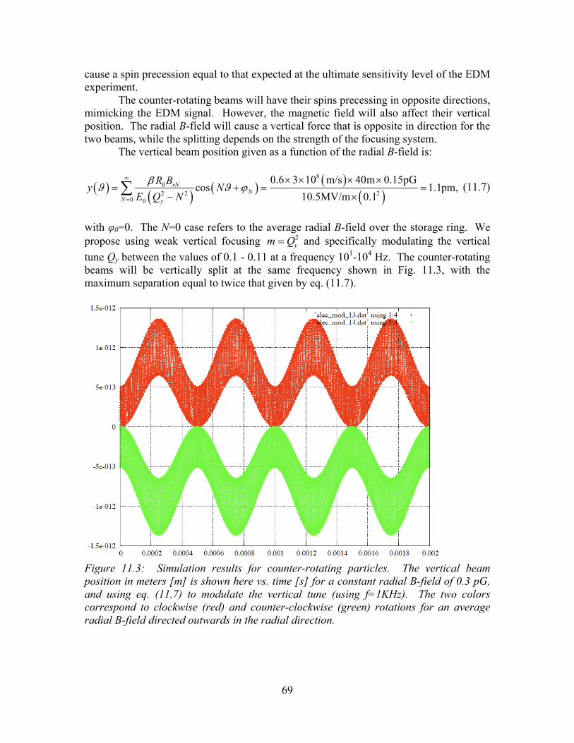
69

cause a spin precession equal to that expected at the ultimate sensitivity level of the EDM experiment.

The counter-rotating beams will have their spins precessing in opposite directions, mimicking the EDM signal. However, the magnetic field will also affect their vertical position. The radial B-field will cause a vertical force that is opposite in direction for the two beams, while the splitting depends on the strength of the focusing system.

The vertical beam position given as a function of the radial B-field is:

802 2 2

0 0

0.6 3 10 m/s 40m 0.15pGcos 1.1pm,

10.5MV/m 0.1rN

NN y

R By N

E Q N

(11.7)

with φ0=0. The N=0 case refers to the average radial B-field over the storage ring. We propose using weak vertical focusing m Qy

2 and specifically modulating the vertical

tune Qy between the values of 0.1 - 0.11 at a frequency 101-104 Hz. The counter-rotating beams will be vertically split at the same frequency shown in Fig. 11.3, with the maximum separation equal to twice that given by eq. (11.7).

Figure 11.3: Simulation results for counter-rotating particles. The vertical beam position in meters [m] is shown here vs. time [s] for a constant radial B-field of 0.3 pG, and using eq. (11.7) to modulate the vertical tune (using f=1KHz). The two colors correspond to clockwise (red) and counter-clockwise (green) rotations for an average radial B-field directed outwards in the radial direction.

70

If the probe is located along the offset between the two beams, then one beam will be at a location r and the other at r1=r+d, while the difference will be

0 0 0

7 -180

1 /2 2 1 / 2

2mA 1.1pm2 2 2 10 2.2 10 T=22 fG.

2 0.02m 0.02m

I I IB d r

r d r d r r

I dB

r r

(11.8)

If we modulate the vertical tune by 10%, the vertical displacement is modulated by 20%, as can be inferred from eq. (11.7). Then the B-field at the modulation frequency is going to be 4.4×10-15 G = 4.4×10-19 T = 0.44×10-3 fT. A low temperature SQUID, commercially available, e.g., from Tristantech (http://www.tristantech.com), has a magnetic field sensitivity of <1fT/√Hz. That means it would take 0.5×107 s, i.e., about half a year of running, for a single SQUID system to achieve S/N=1. Since we expect to have at least 32 SQUIDS in 16 locations around the ring, the S/N should go up by about a factor of 5.

If the beams are offset (displaced) in the horizontal direction, then the residual field is going to point in the vertical direction. We need to have the ability to tell the magnetic field direction in order to differentiate between horizontal and vertical displacements. For this method to work, we need to shield the magnetic field of the ring from the earth’s field as well as noise due to various human activities (see Sections 8 and 9). As noted earlier, we plan to obtain the reduction factor of 109 that we need using:

1) Feedback outside the ring (using Helmholtz coils in the ring tunnel). 2) Passive shielding (we expect a shielding factor of 104 to 105 using three to four

mu-metal layers). 3) Feedback inside the beam tube (using Helmholtz coils).

11.3.2 Geometrical effect due to E-fields In three dimensions, when the spin rotates first about one axis and then about a second one, and then the rotations repeat with opposite sign, the total spin rotation equals the product of the two rotation angles with respect to the third axis. Yuri Orlov did the analytical estimations given in the deuteron EDM proposal [1]. A number of conclusions from studying the effect over the years are:

1) The N=1 is the most dangerous one, in which the B-fields rotate once around the azimuth with a definitive helicity. Also, even though the total sum of the E-field vectors around the ring may equal zero, their effects on the final spin rotations are not zero.

2) The effect has a definitive phase that depends on the ring azimuthal location. The total effect summed up around the ring azimuth is zero. However, at every

71

specific location the effect is non-zero and a specific polarimeter could show a non-zero effect. To protect against the N=1 effect it is sufficient to have two polarimeters around the ring located at diametrically opposite locations.

3) Using four polarimeters around the ring provides enough information to diminish the N=2 effect as well.

The proton spins do not precess in the presence of E-fields alone when their

momentum is “magic.” The geometrical effect due to B-fields present has been analyzed in [2]. As long as the average magnetic fields are below a μG level, the effect will be much below our sensitivity level. Magnetic fields of this level will cause beam splitting (radial B-field) or an asymmetric horizontal spin precession (vertical B-field), which are several orders of magnitude higher than our single store sensitivity. We therefore expect no problem on the geometrical effects issue due to transverse B-fields. Longitudinal B-fields also need to be below a μG level. Those can be probed in separate runs of ~1% of the time by enhancing the transverse beam-polarization by a factor of ten.

Ref. [2], which covers E-fields as well, shows that protons at their “magic” momentum do not have a geometrical effect. Nothing happens when the E-fields and the ring geometric parameters are ideal. However, there are still cases when only E-fields are present and for some reason the proton momentum is not exactly “magic.”

We will now consider E-field plate alignment and placement tolerance. The expected EDM signal, assuming the spin is along the momentum, is estimated in eqs. (11.1) and (11.2). Since the revolution time is of order 1.5 μs, the vertical spin angle would be about 0.01prad/revolution. This is a very small angle and geometrical effects could provide competition to it.

Horizontal betatron oscillations cause energy oscillations at the betatron oscillation frequency. Since the betatron frequency is not the same as the cyclotron frequency, these oscillations cannot combine with a vertical electric field--due to misalignments in the placement of the quads and/or the E-field plates--to produce a first-order geometrical effect. Energy oscillations, however, can also occur if the E-field plates are not aligned with respect to each other and if their centers are not in the same radial position. When the proton beam leaves one set of plates and goes to the next one, its kinetic energy will on average depend on the azimuthal location around the ring. This effect, combined with an undesired vertical E-field, can produce a geometrical effect.

The horizontal spin precession with only the E-field present is

2

,a

q m Ea

m p c

(11.9)

where q=e is the charge of the particle, e the absolute value of the electron charge, m the mass of the particle, p its momentum, its velocity in units of the speed of light c, and E the electric field.

To estimate the order of the horizontal spin precession rate due to momentum offset, we take the derivative of eq. (11.9) as a function of momentum:

72

22

3 2

28

6

2 ... 2

0.9382 0.6 3 10 m/s 10.5MV

938M V 0.7

4 10 rad/s,

aa

a

a

d e m E e m dpd cE

dp m p c mc p p

e dpd

e p

dpd

p

(11.10)

and for dp/p=10-4 we get

4 6 310 4 10 rad/s 0.5 10 rad/s.ad (11.11)

Since the revolution time is about 1.5 μs, the spin precession will be ~1mrad/revolution for dp/p=10-4. This is a potentially significant spin precession, so it is worth looking into the possibility of creating a geometrical effect.

Let us imagine the following geometrical defect: for ¼ of the ring, the average proton kinetic energy changes going from one sector to the next; then for the next ¼ of the ring, the sector plates are rotated with respect to a single plane by about 0.1 mrad, i.e., creating a vertical E-field. Finally, for the next two sectors we get the opposite effects, such that the direction of the fields creates a definitive helicity. Even though the total E-fields and energies are balanced within one revolution, the spin rotations may not be, creating a so-called geometrical effect.

There are 16 straight sections (see Figure 4.4) for which we will assume that the relative E-field plate placement to the same radius is good to 30 μm. Let us also assume that the average plate separation in all sections is the same within ~30 μm, which is 10-3 of the 3 cm plate separation. Finally, let us assume that the voltage on the plates around the ring is the same as or better than 10-4 of itself, so the field-change from section to section will be dominated by the variation in the plate separation and absolute plate placement. Since 10 MV/m requires applying ±150 kV on the plates, ~30 μm variation in plate separation means

6150keV 30 m10 .

233MeV 3cm

(11.12)

The kinetic energy difference, on average, will be ~0.5ppm going from one sector to the next. This corresponds to ~1 ppm in dp/p.

Assuming that this offset is present in about half the ring, the horizontal spin precession is going to be about 10 μrad. In addition, assuming that ¼ of the plates are rotated by 0.1 mrad we will also get about 1 μrad of vertical spin rotation due to the vertical E-field. In the next half of the ring, the spin rotations repeat with the opposite sign this time. The total of the spin rotations in three dimensions will induce a combined spin rotation with respect to a longitudinal axis equal to the product of the two rotations, i.e., 10-10 rad/revolution. If the average spin direction is along the longitudinal axis

73

within 10mrad, the final vertical spin rotation will be 10-13 rad/revolution, which is ~10 times the projected EDM effect.

However, the vertical E-field will cause a significant orbit distortion [3]:

0 002 2

00

sin 4mm sin / ,NN

y

a R Nsy s R

RE N Q

(11.13)

where s is the longitudinal path length, R0 the ring radius and a01/E0=0.1 mrad (the E-field misalignment with respect to a plane). Qy = 0.2 is the vertical tune. The orbit plane around the ring can be easily defined to ~25 μm. Therefore, the plate misalignment a01/E0 can be reduced by a factor of ~102 to 1 μrad by using beam-based alignment. The geometrical effect will be well below the EDM sensitivity level.

Polarimeters located halfway around the ring will have an opposite geometrical phase sign; adding their signal will eliminate this background to a high degree. Similarly, CW-CCW beams will have a sign signal opposite to their EDM effect, reducing the effect even further. Even though it looks like the geometrical phase effect is well under control, we may still find it advantageous to use two to four polarimeters located at specific azimuthal locations to probe any residual geometrical phase effect. 11.3.3 Fields from the counter-rotating beams. If the two beams do not overlap completely, on average they will feel a vertical force from each other that is opposite in direction for the two counter-rotating beams and will depend on beam intensity. However, those fields are proportional to the beam separation and are not a problem as long as the BPMs are sensitive to the beam separation and feedback is used to eliminate that signal. They only serve to shift the calibration between the beam separation and the net radial B-field as a function of beam intensity. 11.3.4 Fields due to E-field in the RF-cavity. This will be a concern if there is energy loss around the ring and it is compensated by the E-field in the RF-cavity. Let us say we have one stripline detector around the ring, in which case the longitudinal impedance will be 25 . Then, for our maximum beam current of 2 mA, the total energy loss per particle and per rotation will be ~0.05 eV. Each proton has a kinetic energy of 232 MeV, so 0.05 eV energy loss is negligible (below 10-9). However, this energy loss is compensated by the electric field in the RF-cavity. If the longitudinal direction of the RF-cavity is rotated vertically, then a net vertical E-field can be present. The sign of this vertical E-field will be opposite for the counter-rotating beams, since their RF phase difference is 180. The vertical fields in that case will not cancel, but will cause beam splitting. The level of the systematic error is irrespective of the length of the cavity; it only depends on the energy loss. The vertical E-field can be estimated:

-4

/(total E-field plate length equal to ~250 m)=

0.05 V /250 m=2 10 V/m.

V rfE E l

(11.14)

74

The vertical offset depends on the vertical tune. We estimate the magnetic field equivalent of this field to be 0.7pG for a longitudinal impedance of 25 . We can assume that on average < 1 mrad, which means the total longitudinal impedance should be kept below 10 k.

Overall, the systematic errors we can think of will be well under control. More systematic error studies based on tracking will be done as the CD-process moves forward. References

1. Yuri Orlov’s estimation of the effect of consecutive rotations through perpendicular axes, included in the deuteron EDM proposal: AGS Proposal: Search for a permanent electric dipole moment of the deuteron nucleus at the 10-29 ecm level, April 2008, available at http://www.bnl.gov/edm/

2. Y.K. Semertzidis, Geometrical Phases and Ramsey-Bloch-Siegert Effect, Internal EDM note, April 2011.

3. W.M. Morse, Geometric Phase Systematic Error, Internal EDM note, September 2011.

75

12. R&D: EXPERIMENTAL ISSUES, COSTS, TIMELINE, AND GOALS

12.1 Main experimental issues The main systematic error effort is concentrated on ways to probe and reduce the background magnetic field. To achieve this goal we propose using a modulated vertical tune that will induce the counter-rotating beams to separate at the same frequency, and using BPMs capable of detecting this separation. The main experimental issues together with their relation to the current state-of-the-art are:

1) A very small vertical offset between the two beams. The offset needs to be on the order of ~1pm averaged over the duration of the experiment. This requires BPMs with a relative position resolution of the order of ~10 nm and BW of 1 Hz. The state of the art today is ~10 nm for a single beam and a single pass with 1010 particles, using resonant cavities. Most of this development was accomplished as part of the ILC R&D [1]. Other types of BPMs, e.g., buttons, have a resolution of 200nm/turn for a 500 mA stored beam, which would translate to 2m/turn for a 5mA beam (see Appendix 8). Their stability requirement over 8 hours is 200nm, which has recently been achieved [2] using 0.1 C temperature stabilized electronics racks. Our requirement is only 10 m/turn for a 2 mA stored beam, while our stability requirements are much more relaxed since we measure a relative beam separation with the same BPM. Considering the potential systematic errors, we have chosen to take a more conservative approach and use magnetometers capable of sensing the (near-DC) beam separation. State-of-the-art magnetometers, either SQUIDS or atomic optical magnetometers, are sensitive at the required level.

2) SCT of the order of 103s or about 109 turns. The best performance was achieved at Novosibirsk for ~107 turns for an electron/positron machine [3]. Our specially designed E-field ring is capable of improving on that by the required factor of 102 (see Section 6).

3) Internal polarimeters with small systematic errors. Similar systems have been developed, but never for a storage ring. We expect the stability of the beam position will completely eliminate this error. Our recent work at COSY demonstrated that we can achieve the polarimeter systematic error goals.

4) Sufficient electric field strengths for large surface areas. A similar system was in operation at Fermilab as part of the Tevatron, where they applied up to ±180 kV for 5 cm plate separation. We expect to reach a similar voltage for 3 cm plate separation by using high-pressure water rinsing, which was shown to give the needed improvement.

5) Beam-beam and spin-spin effects. Ours are negligible because our effective luminosity is moderate (a few × 1026/cm2-s).

6) Simulation software to track spin and particle momentum in a storage ring that includes E-fields. The simulation needs to include at least the second-order beam dynamics effects as well as the fact that particle motion in the E-field region significantly changes particle momentum.

76

12.2 Estimated costs We believe that we can develop prototypes for several of the major ring systems within a two-year R&D period. Their costs are are estimated in Table 12.1: $2M over 2 years. These estimates cover equipment fabrication and installation at an accelerator facility, as well as full-time post-doctoral researchers. They do not cover the salaries of the staff researchers working on these projects, even though it is clear that several professionals will be required.

The cost of the spin coherence time study depends on what is learned about the capabilities of magnets already installed at COSY. It includes expenses for additional magnets or rewiring the existing set of 18 sextupoles, any changes needed to the RF-solenoid for proton operation, and new expenses for constructing a stochastic cooling system to operate at velocities well below the speed of light. The polarimeter work will begin with detector commissioning in a new scattering station on the external beam line, and the assembly of a prototype with data acquisition equipment, in order to repeat the systematic error calibration for the angle region of the proton experiment. Also required is a solid target system for the WASA detector in order to obtain broad spectrum measurements of proton and deuteron-induced reactions on carbon. Table 12.1. Estimated costs of developing several major ring system prototypes over two years. Total $2M (salaries of staff researchers not included).

System Total amount requested Comments Spin Coherence Time $0.4 M Benchmarking of simulation

software with polarized stored beams at COSY.

Beam Position Monitors $0.6 M Testing in RHIC is planned. E-field $0.4 M Prototype testing at BNL. The

required E-field is 10.5 MV/m with a plate separation of 3 cm.

Polarimeter $0.6 M Internal polarimeter development for the pEDM experiment.

12.3 R&D timeline

The technically-driven timeline for the R&D described above is:

Two years R&D (dark blue) One year final ring design (green)

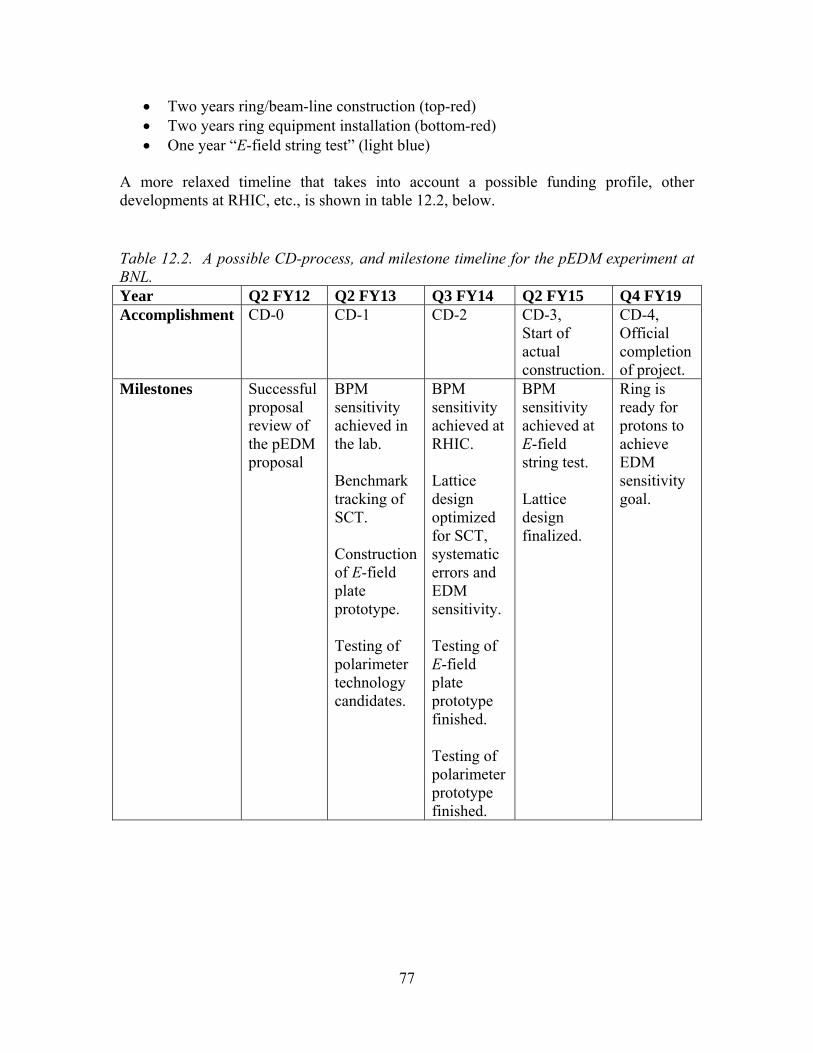
77

Two years ring/beam-line construction (top-red) Two years ring equipment installation (bottom-red) One year “E-field string test” (light blue)

A more relaxed timeline that takes into account a possible funding profile, other developments at RHIC, etc., is shown in table 12.2, below. Table 12.2. A possible CD-process, and milestone timeline for the pEDM experiment at BNL. Year Q2 FY12 Q2 FY13 Q3 FY14 Q2 FY15 Q4 FY19 Accomplishment CD-0 CD-1 CD-2 CD-3,

Start of actual construction.

CD-4, Official completion of project.

Milestones Successful proposal review of the pEDM proposal

BPM sensitivity achieved in the lab. Benchmark tracking of SCT. Construction of E-field plate prototype. Testing of polarimeter technology candidates.

BPM sensitivity achieved at RHIC. Lattice design optimized for SCT, systematic errors and EDM sensitivity. Testing of E-field plate prototype finished. Testing of polarimeter prototype finished.

BPM sensitivity achieved at E-field string test. Lattice design finalized.

Ring is ready for protons to achieve EDM sensitivity goal.

78

12.4 Comments about R&D plans 1. The electric field goal is to have the E-field plates separated by 3 cm and obtain a

field of 10.5 MV/m by applying a field of about ±150 kV. In the FNAL Tevatron, the electro-static separators operate reliably at the same voltage for 5 cm separation. We believe that recent advances in metal surface treatments will provide the needed improvement, and then some more. Absent that, we will either change the ring radius or reduce the plate separation. (The former will cost more, and the latter will require running longer because of the smaller acceptance.)

2. We have developed one reliable particle-tracking program indicating that 103 s storage time is possible. We are currently working on applying stochastic cooling to further prolong the SCT and provide the possibility of compensating for any loss in statistics due to, e.g., lowering the E-field strength goal. It will also provide the impetus for an upgrade and further statistical improvement by another order of magnitude over the current goal.

3. Polarimeter work on the systematic errors has finished. We have proven the expected polarimeter-related systematic errors to be more than a couple of orders of magnitude below our statistical sensitivity. The technology to be used in the polarimeter detector is a very active part of the ATLAS upgrade R&D (micro-megas) and of the ALICE detector (MRPC). The ATLAS R&D already has achieved a couple of orders of magnitude higher data-taking rate than is required for the proton EDM experiment, while they have also eliminated the dead-time of the detector due to a possible spark. The electronics under development can also be used for the proton EDM experiment with very minor modifications. We do not expect any surprises in this R&D effort.

4. Since the BPM sensitivity level will define the ultimate sensitivity of the experiment, BPM development is ultimately the most important R&D component. It is also the one requiring the most care. Thus, after being designed in detail, it will be built and tested in the lab first, then in RHIC, and finally in an E-field string test. The string test will cover a section of the ring lattice--including the RF system--to establish that the separate systems can work together harmoniously. (With that established, the actual experiment can be built.) We will develop at least one alternative technology to the BPM magnetometers, which we plan to test in parallel.

References

1. Y. Inoue et al., PRST-AB 11, 062801 (2008); S. Walston et al., Nucl. Instrum. Meth. A578, 1 (2007).

2. Kurt Vetter, private communication and C-AD talk of February 18, 2011. 3. I.B. Vasserman et al., Phys. Lett. B187, 172 (1987); Phys. Lett. B198, 302

(1987); A.P. Lysenko et al., Part. Accel. 18, 215 (1986).

79

13. COST OF THE EXPERIMENT At BNL there are two candidate locations for the proton EDM ring. One, at the extension of the AGS to RHIC transfer line (ATR), locally referred to as North Area, would require building a new ring-tunnel for the ring and a beam-line. The other location is at the former slow beam extraction (SEB), locally known as East Area. The existing building can cover most of the ring, requiring some extensions to cover it completely. Most of the cost at this location is due to clean-up requirements.

To estimate the cost of the experiment, we held weekly meetings with collider-accelerator department (C-AD) engineers over the course of several months. We discussed the specs required by the systems and the available options meeting them. The engineers then came up with the cost, including large-project indirect charges by the lab, which for a single invoice is 17.55% for up to $0.6M. An average contingency of more than 50% was used for most system costs, including those estimated by outside companies. Value engineering can reduce this large contingency; defining the scope and specs of the various systems will reduce the cost uncertainty.

The experiment’s cost as estimated mainly by C-AD personnel is given in Tables 13.1 and 13.2, below, and in more detail in Tables 13.3 - 13.7. In summary, the cost of the EDM ring itself is $25.6M, including indirect costs. Including contingency raises its cost to $39.5M, see Tables 13.1, 13.2 and 13.3. The ring tunnel (conventional) and the beam-line total costs depend on the location of the ring: $29.2M with the ring at ATR and $22.6M at SEB, including indirects and contingency. Hence, the total EDM experiment cost ranges between $62.1M and $68.7M, depending on location. Table 13.1 Comparative estimated costs of the proton EDM experiment at ATR and SEB, including BNL indirect costs but excluding contingency. System Experiment w/

indirects Conventional plus beamline w/ indirects

Total

pEDM at ATR $25.6M $20M $45.6M

pEDM at SEB $25.6M $14M $39.6M Table 13.2 Comparative estimated costs of the proton EDM experiment at ATR and SEB, including both BNL indirect costs and contingency. System Experiment w/

indirects and contingency

Conventional & Beamline w/ indirects and contingency

Total

pEDM at ATR $39.5M $29.2M* $68.7M

pEDM at SEB $39.5M $22.6M** $62.1M

* See Tables 13.4-13.5 for details. ** See Tables 13.6-13.7 for details.

80

Table 13.3 Estimated costs of the pEDM experiment at either ATR or SEB: some details. HPR refers to high-pressure water rinsing. System Cost W/

Indirects Contingency Total Source

Electrical $4.3M 50% $6.45M C-AD V.C. + plates + Vacuum + HPR

$5.7M 10-50% $7M C-AD

Magnetic shielding

$5.6M 17.55% (up to $0.6M)

50% $8.56M Amuneal company

Installation of M.S.

$0.860M 17.55% (up to $0.6M)

50% $1.45M Amuneal company

Polarimeter $0.6M 17.55% 50% $1.06M pEDM Active magn. feed. $732K 100% $1.46M C-AD Controls $876.5K 100% $1.75M C-AD Control room $250K 100% $0.5M C-AD Installation $3.7M 100% $7.4M C-AD SQUID-BPM $2.5M 17.55% (up

to $0.6M) 50% $3.91M pEDM

Total $39.5M

81

Table 13.4 Estimated costs of building new ring tunnel at ATR. System Cost W/ Indirects Contingency Total Source Site Utilities $165.9K 45% C-AD pEDM ring & services

$7,282.9K 45% C-AD

Service buildings & utilities

$671.3K 45% C-AD

Beam transport, service buildings & utilities

$810.7K 45% C-AD

Architectural, engineering & construction Services

$2,014.5K 45% C-AD

Total 12,587.1K $5,664.2K $18,251.3K Table 13.5 Estimated costs of beam-line at ATR. System Cost w/small

project ind. (SPI)

W/ large project Indirects (LPI)

Contingency Total Source

Electrical distribution & tray runs

$502.8K 50% C-AD

Magnets $2,215.4K 50% C-AD

Power supplies $1,362.5K 50% C-AD

Vacuum system $744K 50% C-AD

Access controls $152.6K 50% C-AD

Instr. & controls $1,594.3K 50% C-AD

Water cooling $302.3K 50% C-AD

Installation labor

$1,103.4K 50% C-AD

Total 7,302.5K $3,651.2K $10,953.7K

82

Table 13.6 Estimated costs of re-purposing ring at SEB. System Cost w/ SPI W/ LPI Contingency Total Source

Removals $5,543.3K $4773.8K 65% $7876.8K C-AD

Utilities $776.83K 65% C-AD

Ring shielding & installation

$2,641.9K 65% C-AD

Misc. $1,366.7K 65% C-AD

Total 8,894.9K $5,781.7K $14,676.6K

Table 13.7 Estimated costs of beam-line at SEB. System Cost w/ SPI W/ LPI Contingency Total Source

Extraction $430.16K 50% C-AD

Magnets $748.12K 50% C-AD

Power supplies $564.86K 50% C-AD

Vacuum system $685.97K 50% C-AD

Access controls $800.13K 50% C-AD

Instr. & controls $779.76K 50% C-AD

Water cooling $295.25K 50% C-AD

Installation labor $1,249.9K 50% C-AD

AC power $232.33K 50% C-AD

Removals $460.55K 50% C-AD

Total $5,267.9K $2,634.0K $7,901.9K

83

ACKNOWLEDGEMENTS We are indebted to the associate lab director for Nuclear and Particle Physics at BNL, Steve Vigdor, for his support and guidance throughout the long development of the storage ring EDM method and for his many important comments on the structure of this proposal. We also thank Sidney Orlov, who has greatly improved its clarity.