90
Prototype Development of an A-Mode Ultrasound Based Intrafraction Motion Management System ABEBE HAILU FREDRIK LUNDQVIST Master of Science Thesis in Medical Engineering Stockholm 2013

i
Prototype Development of an A-Mode Ultrasound Based
Intrafraction Motion
Management System
ABEBE HA ILU
FREDR IK LUNDQVIST
Master of Science Thesis in Medical Engineering
Stockholm 2013

ii
iii
This master thesis project was performed in collaboration with
Elekta Instrument AB
Supervisor at Elekta: Ola Svärm
Prototype Development of an A-mode Ultrasound Based Intrafraction Motion
Management System
Prototyputveckling av ett A-mode ultraljudsbaserat intrafraktionellt
rörelsehanteringssystem
ABEBE HAILU
FREDRIK LUNDQVIST
Master of Science Thesis in Medical Engineering
Advanced level (second cycle), 30 credits
Supervisor at KTH: Nils Holmström
Examiner: Massimiliano Colarieti-Tosti
School of Technology and Health
TRITA-STH. EX 2013:94
Royal Institute of Technology
KTH STH
SE-141 86 Flemingsberg, Sweden
http://www.kth.se/sth

iv

v
ABSTRACT
Owing to the steep dose fall-off curves of high precision and accuracy radiation therapy (RT)
modalities such as stereotactic body RT (SBRT), treatment plans with extraordinarily small
margins to organs at risk (OARs), such as the spinal cord, has been made possible. With this
development, patient movements during treatment, i.e. intrafraction motion (IFM), must be
monitored more closely. This master thesis was aimed at developing an A-mode ultrasound
prototype to detect the motions of the cervical spine as part of an IFM management (IFMM)
system. Current IFMM systems have several drawbacks, including invasiveness and indirect
measurements.
The existing prototype was tested in order to identify areas of improvement. The prototype
developed was equipped with a preconditioning circuit that retains the frequency information
of the signal. Furthermore, software was developed based on wavelet filtering and enveloping
using the Hilbert transform. Multiple logic algorithms were added in order to handle lost
signals, competing echoes, echoes from soft tissues etc.
The newly-developed prototype was found to have higher accuracy and precision than the
pre-existing prototype. It was also more robust when measuring distance to the spine. A
difficulty in segmenting the echo for bone arises for low quality signals. Therefore a
compromise exists between setup time, including probe adjustment, and signal quality. Future
work includes the manufacturing of a new neck rest to enable robust probe adjustment and
fixation.

vi

vii
SAMMANFATTNING
I dag fås skarpa dosfördelningskurvor från strålterapimodaliteter med hög precision och
träffsäkerhet, d.v.s. sådana som används vid stereotaktisk kroppsstrålterapi. Detta har
inneburit behandlingsplaner med ovanligt små marginaler till högriskorgan såsom
ryggmärgen. Denna utveckling innebär att patientrörelser under behandlingen,
intrafraktionella rörelser, måste övervakas noggrannare. Målet med detta examensarbete på
masternivå var att utveckla en prototyp för att detektera rörelser av den cervikala ryggraden.
Detta gjordes med hjälp av A-mode ultraljud som del av ett intrafraktionellt rörelsesystem.
Befintliga system har flera nackdelar såsom invasivitet och indirekta mätningar.
Den existerande prototypen testades för att identifiera förbättringsområden. En krets
utvecklades för att bevara frekvensinnehållet i signalen. Mjukvaran baserades på
waveletfiltrering och signalomslutning med hjälp av hilberttransformen. Flera logikalgoritmer
implementerades för att hantera tappade signaler, konkurrerande ekon, ekon från mjukvävnad
etc.
Den nyutvecklade prototypen visade sig ha högre precision och träffsäkerhet än den befintliga
prototypen. Den var även mer robust vid avståndsmätningar till ryggraden. För signaler av låg
kvalitet uppstår en svårighet i att segmentera ekot för ben. En kompromiss krävs därför
mellan inställningstiden, vilket inkluderar riktning av transducern, och signalkvalitet.
Framtida arbete inkluderar tillverkning av ett nytt nackstöd för att möjliggöra fastfästning och
riktning av transducern.

viii

ix
ACKNOWLEDEGEMENTS
We would like to express our appreciation to Malcolm Williams, Electronics Designer,
Markus Nyman, Mechanical Engineer, and Björn Nutti, Software Engineer, for the valuable
support they provided during this project. We also want to offer our special thanks to Systems
Engineer Rui Chen for giving us the opportunity to go on this astonishing journey of
development at Elekta Instrument AB.
Finally, we want to thank our supervisors Ola Svärm and Nils Holmström at Elekta
Instrument AB and the Royal Institute of Technology, respectively.
Abebe Hailu & Fredrik Lundqvist
Stockholm, Sweden
May 2013

x

xi
SYMBOLS AND ABBREVIATIONS
Symbols
Symbol Meaning
Av Voltage amplification
a Wavelet scaling factor
CPV Cauchy principle value
Cx Capacitor x [F]
c Speed of sound [m/s]
d Echo distance [m]
Fs Sampling frequency [Hz]
f Frequency instant
f0 Ultrasound frequency [MHz]
fcH High-pass filter cutoff frequency
fcL Low-pass filter cutoff frequency
i Index
N Number of wavelet coefficients
R Acoustic reflection [%]
Rx Resistor x [Ω]
SR Slew rate [V/µs]
T Wavelet threshold
t Time instant
Z Acoustic impedance [106·kg/m
2s]
α Attenuation coefficient [dB/cm]
ρ Density [kg/m3]
σ(MAD) MAD standard deviation estimate

xii
Abbreviations
Abbreviation Meaning
1D/2D/3D one/two/three-dimensional
A-mode Amplitude mode
ADC Analog-to-Digital Converter
C1-C7 Cervical vertebra 1-7
CBCT Cone Beam Computed Tomography
CPU Central Processing Unit
CTV Clinical Target Volume
DSP Digital Signal Processor
FIFO First In, First Out
FFT Fast Fourier Transform
FPGA Field-Programmable Gate Array
GPIO General Purpose Input Output
GTV Gross Tumor Volume
GUI Graphical User Interface
HP High-Pass
HT Hilbert Transform
I/O Input/Output
IFMM IntraFraction Motion Management
IR InfraRed
LP Low-Pass
MAD Median Absolute Deviation
MSPS Mega Samples Per Second
OAR Organ At Risk
RT Radiation Therapy
SBRT Stereotactic Body Radiation Therapy
SNR Signal-to-Noise Ratio
STD STandard Deviation
TGC Time Gain Compensation
US UltraSound
WT Wavelet Transform

xiii
CONTENT
1. INTRODUCTION ........................................................................................................................................ 1
1.1 BACKGROUND ...................................................................................................................................... 1 1.2 PROBLEM DESCRIPTION ........................................................................................................................ 1 1.3 ELEKTA AB .......................................................................................................................................... 1
2. OBJECTIVES............................................................................................................................................... 3
2.1 AIM ....................................................................................................................................................... 3 2.2 DEMARCATIONS.................................................................................................................................... 3
3. METHODOLOGY ....................................................................................................................................... 5
4. THEORETICAL FRAMEWORK .............................................................................................................. 7
4.1 ANATOMY OF THE SPINE AND NECK ..................................................................................................... 7 4.2 EXTERNAL BEAM RADIATION THERAPY ............................................................................................... 9 4.3 INTRODUCTORY ULTRASOUND THEORY ..............................................................................................14 4.4 EMBEDDED SYSTEMS ...........................................................................................................................18
5. PROTOTYPE DEVELOPMENT ..............................................................................................................23
5.1 ORIGINAL PROTOTYPE .........................................................................................................................23 5.2 CIRCUIT DESIGN ..................................................................................................................................30 5.3 ALGORITHM DEVELOPMENT ................................................................................................................32 5.4 FINAL PROTOTYPE ...............................................................................................................................41
6. RESULTS .....................................................................................................................................................49
7. DISCUSSION ..............................................................................................................................................51
7.1 SOLUTION DRAWBACKS ......................................................................................................................51 7.2 SYSTEM ERRORS ..................................................................................................................................52 7.3 DEVELOPMENT COMPROMISES ............................................................................................................52
8. CONCLUSIONS ..........................................................................................................................................55
9. FUTURE WORK ........................................................................................................................................57
REFERENCES ................................................................................................................................................59
APPENDIX A: PROTOTYPE SPECIFICATIONS .....................................................................................63
APPENDIX B: TEST PROTOCOL ...............................................................................................................66
APPENDIX C: CIRCUIT CALCULATIONS ..............................................................................................69
APPENDIX D: EVALUATED ALGORITHMS...........................................................................................72
APPENDIX E: SOURCE CODE ...................................................................................................................73

xiv

1
1. INTRODUCTION
1.1 Background With the development of radiation therapy (RT), techniques have been developed where high
dose fall-off, accuracy and precision are obtained to ensure tumor eradication. However, with
these techniques, the importance of patient fixation and monitoring of movements has
increased due to the higher dose to the target with smaller margin to healthy tissues. For
intracranial targets such as brain metastases, stereotactic radiosurgery (SRS) is a well
established technique in which the tumor is irradiated with a high conformal dose to eradicate
all tumor cells in one treatment delivery. Traditionally, this is done with a frame attached to
the skull to form an external coordinate system with which the radiation beams are
coordinated.
Presently evolving modalities enable SRS to be done with extracranial targets. Common
tumor and metastatic sites are the lung, prostate and spine. With these techniques, no external
frame allows such high immobilization as with intracranial SRT. The additional factor of
movements from breathing during treatment delivery must also be taken into account.
Current system solutions to handle movements during treatment delivery (intrafraction motion
management, IFMM) may use surface detection laser or fiducial markers inside or on the
surface of the body. When motions are detected, the operator is warned to halt the procedure.
A major drawback is however the basic assumption that movement of fiducials or the
patient’s skin would correspond to movement of the tumor or organ of interest. Other
solutions, such as image guided systems with built in x-ray modules, can position the patient
and confirm the setup, but these systems are of no assistance for real-time motion tracking.
1.2 Problem description Because there are no qualified ways of directly tracking the spine during treatment, and
because of the highly sensitive nearby healthy tissues (such as the spinal cord), this master
thesis was about developing an amplitude mode (A-mode) ultrasound (US) prototype to
measure the distance to the cervical spine.
The prototype developed should give deeper knowledge about whether or not the concept of
US IFMM holds. The data obtained can be used to monitor the movement of the spine and
allow irradiation halts (gating) during treatment delivery. If the prototype proves to be
successful, this non-invasive and radiation-free technique has the ability to enable real-time
tracking and radiation beam adaption relative to the spine during treatment delivery. For this
prototype, only the cervical spine was focused on. For future iterations the prototype may be
expanded to monitor other parts of the spine.
1.3 Elekta AB Elekta is a medical technology company with clinical solutions for the treatment of cancer
and brain disorders. It was founded in 1972 by neurosurgeon and Professor Lars Leksell, the
inventor of the Leksell Gamma Knife. Today, Elekta products are used in over 6000 hospitals
around the world and were part of the treatment of almost one million patients in the year of

2
2011/12. The company is active in four related areas; neuroscience, oncology, brachytherapy
and software [1]. The work described in this report was made for and in cooperation with
Elekta.

3
2. OBJECTIVES
2.1 Aim Due to the fact that this technique is not tested in a clinical setting, the aim was primarily to
develop an A-mode US prototype with the ability to robustly measure the distance to the
cervical spine in real-time for a patient in a supine position. The prototype would also
measure relative distances to a reference point, i.e. motions. If proven to be successful, the
prototype will eventually be used during radiation treatments to evaluate the clinical
usefulness of the technique.
A simple prototype for this purpose already existed, but had not been thoroughly tested. As
part of the aim previously mentioned, the objective was to develop a new prototype that
covers the areas of weakness of the existing prototype, in terms of hardware and software, to
meet the performance needed to be successful in real clinical testing. The aim was divided
into
design of a pre-conditioning circuit for improved signal acquisition
development of a robust echo detection algorithm
implementation of the algorithm on a suitable embedded system
assembling of an enclosure for the prototype with appropriate connection ports.
2.2 Demarcations The neck rest needed to form the connection between the US probe and patient was not to be
manufactured as part of this master thesis. There is however a neck rest prototype, without
sufficient probe fixation, that was used to some extent in testing.
The distance measurements to the spine were restricted to the cervical spine. Future
improvements may be added with an expanded view if the prototype proves successful.
Only the current US probe was used in the prototype. No further tests than the ones already
conducted were made on this probe. Movements are only detected axially in respect to the
probe and, consequently, the prototype has 1D functionality. Lateral movements will not be
correctly interpreted until the prototype is expanded with more probes to gain 2D or 3D
readings.
Tests of a more clinical nature were performed on two human subjects.

4
5
3. METHODOLOGY
The project was divided into the following phases:
1. Testing of existing prototype
2. Literature study
3. Prototype development
i. Signal acquisition
ii. Echo detection algorithm
iii. Embedded system implementation
iv. Hardware design
4. Testing and verification
The project thus had distinct phases with different methods to be applied. Phase 1 was
performed with the design of a test rig. Different tests were decided upon to enable
comparisons between prototypes and to show accuracy and reliability in clinical situations.
This phase hence provided the test protocols to be used in phase 4. The experiences with the
prototype and its limitations were of use in the following literature study.
The literature study of phase 2 was conducted by searching for scientific articles in the area of
this master thesis. Books and other resources were mainly used for review of more
fundamental facts. The literature study covered all aspects of the project, but further phase
specific reviews were planned to take place in the beginning of each phase.
Phase 3:i contained the implementation of a better circuit to obtain a low noise and low
distortion signal as input to the embedded system. The circuit was simulated in Cadence
OrCAD PSpice and LTspice before implementation. The main aim of the software algorithm
of phase 3:ii was to find the echo from the cervical spine present in the US signal in order to
calculate the distance to it. Phase 3:ii focused on what combination of algorithms to use. The
goal of this phase was to obtain MATLAB prototypes and, by a series of tests, to choose the
most appropriate. In phase 3:iii, the migration from MATLAB prototypes to an embedded
system was made. Which system to use was decided in phase 3:ii based on shipping times.
The overall hardware design, where all parts were tied together, was done in phase 3:iv. The
end result was defined to be a mobile box with suitable input ports. An important aspect was
to avoid noise in the signal by using isolated cables and small electrical components in the
final circuit.
Phase 4 was similar to phase 1 with the same testing protocol, but with further focus on
clinical use. Henceforth in this thesis, the term clinical tests will refer to tests on human
subjects. These tests included testing of the prototype on a human subject in a supine position
with a neck rest. However, less stringent tests, sometimes done on the arm without any probe
support, were also performed during the software implementation in order to find appropriate
parameter values. Observe that the term clinical test is used only to separate the types of tests
performed on the prototype, they should not be compared to the highly controlled clinical
tests normally conducted when developing a new product.

6

7
4. THEORETICAL FRAMEWORK
4.1 Anatomy of the Spine and Neck This section contains spine and neck anatomy relevant for the thesis.
The human vertebral column (Figure 1), also called the spine, is a flexuous and flexible
column consisting of 33 bones called vertebrae. The vertebrae are grouped and named as
cervical, thoracic, lumbar, sacral or coccygeal vertebrae according to the region in which they
are located. Some literature mention only 24 vertebrae, since nine vertebrae in the sacrum and
coccyx are considered fused in adult humans. The upper two thirds of the spine hold the
spinal cord within the vertebrae’s cavities [2].
Figure 1. A lateral view of the spine. Intervertebral discs holding the spine together can be seen between the vertebrae [2].

8
The cervical spine is defined as the first seven vertebrae of the spine. The cervical curvature
(see upper part of Figure 1) is less marked than for the other regions of the spine. The cervical
vertebrae are commonly named C1-C7 according to their position in the spine. The C1
vertebra (also referred to as atlas) links the skull to the spine and is therefore different in
anatomy than the other vertebrae. Furthermore, C2 (also referred to as axis) and C7 differ
from C3-C6. Anatomy common to C3-C7 is the spinous process (the posterior sharp point of
the vertebra) the transverse process (the lateral structures of the vertebra) and the lamina (the
plate fusing the spinous process with the vertebra) (see Figure 2) [2].
Figure 2. A C3-C6 cervical vertebra showing the transverse process, lamina and the spinous process (found posterior on the
spine). The spinal cord runs through the center cavity of the vertebra [2].
The most prominent lateral and posterior structures of the cervical vertebrae are a variety of
different muscles (see Figure 3).
Figure 3. The posterior muscles of the neck and upper back (left), and lateral muscles of the neck (right) [2].
The area between the sternocleidomastoid and trapezius muscle is called the posterior triangle
[2]. A transverse slice of the soft tissue anatomy in the neck can be seen in Figure 4.

9
Figure 4. A transverse slice of the soft tissue surrounding the lower cervical vertebrae. Original image with courtesy of
Florida Center for Instructional Technology.
4.2 External Beam Radiation Therapy RT is one of three modalities used in the treatment of cancer, the others being surgery and
chemotherapy. External beam RT refers to techniques where the target tissue in the patient is
externally radiated with ionizing radiation. The goal of a RT treatment is to eradicate the
tumor, while sparing healthy tissue as much as possible. Oncologists also speak of tumor
control, meaning the extinction of clonogenic tumor cells after full treatment [3].
Different types of radiation may be used such as photons, electrons or ions. A property they
all have in common is that ionizing radiation kills cells by rendering damage to DNA. For the
area investigated in this work, photons are of greatest relevance. To acquire a photon beam
used for RT, most systems use a linear accelerator (LINAC) [3].
Today, a routine RT modality in clinical practice with high conformality to the target is called
three-dimensional conformal radiation therapy (3DCRT). It is based on a treatment planning
scheme in 3D, in which the patient anatomy and tumor are delineated. During treatment, the
target is irradiated with a number of radiation beams from different angles according to this
plan. The beam profiles are shaped for every angle to match the geometry according to the
treatment plan [3, 4]. The graphical user interface (GUI) of a treatment planning system is
shown in Figure 5.
Trachea
Sternocleidomastoid muscle
Trapezius muscle
Subcutaneous tissue
Cervical vertebra
Fat

10
Figure 5. The dose distributions shown in a treatment planning software. The graphs in the top right square are the dose
curves showing dose levels to clinical volumes. Courtesy of Elekta.
RT is normally performed in multiple treatment sessions, called fractions. The rationale for
fractionation is traditionally based on what is known as the four R’s (reoxygenation, repair,
redistribution and repopulation). These will not be explained further; however, of interest to
this work specifically is the property of cell repair. Fractionation is partly justified by the fact
that a quantity of healthy tissue is irradiated during treatment delivery (noticeable in Figure 5).
By giving the treatment in fractions, the healthy tissue is given the ability to repair sublethal
damage between sessions [3, 4].
4.2.1 Simulation Imaging and Treatment Planning The purpose of simulation imaging and treatment planning is to designate the target or targets
based on patient anatomy, find critical structures and determine an optimal approach to
treatment delivery, including dose calculations. Imaging of the patient during treatment
planning (commonly referred to as simulation imaging) is done by CT, MRI or PET (PET
images may be fused with CT or MRI images). During simulation imaging, the patient is
immobilized in the position to be used during treatment delivery. Factors to be aware of are
breathing and other movements of the patient. For some RT modalities the patient is highly
immobilized and the breathing cycle is correlated to match the imaging process. Abdominal
compression may also be applied to reduce movements due to breathing [3, 4, 5].
During the treatment planning process, several volumes are defined and delineated in the
treatment planning software in 3D. These can be seen in Table 1.

11
Table 1. Definitions of volumes used during treatment planning and treatment delivery [3].
Volume Full Name Definition
GTV Gross Tumor Volume The extent of palpable/visible malignant growth.
CTV Clinical Target Volume
In addition to the GTV, the CTV also includes
adjacent microscopic malignant disease in need of
treatment.
ITV Internal Target Volume
In addition to the CTV, an internal margin is added
to account for positional changes of the CTV due
to organ motions such as breathing.
PTV Planning Target Volume
In addition to the ITV, an external margin is added
to account for setup uncertainties, machine
tolerances and intra-treatment variations.
OAR Organ At Risk An organ for which a treatment dosage is a
significant fraction of that organ’s tolerance.
Hence, due to uncertainties, for every treatment planning, margins need to be added to the
GTV in order to ensure tumor control after full treatment. These margins are partly dependent
on the machine at hand but also the available control of changes in patient position both
during treatments (intrafraction) and between treatments (interfraction) [3, 4, 5]. If a perfect
immobilization and position reproducibility of the patient exists, there would be no need of
the ITV and PTV.
4.2.2 Intra- and Interfraction Motion and Implications Intrafraction motion is defined as movement of the tumor during treatment delivery. It can
thus both derive from normal physiological functions or from patient movements.
Intrafraction motion may for example originate from breathing, swallowing or muscle
tensions. The importance of intrafraction monitoring thus increases with treatment time. It
then follows that interfraction motion is movement of the tumor from treatment to treatment.
It can be due to for example imprecise patient repositioning or tumor shrinkage [4].
The hazard of intra- and interfraction motion is irradiation of healthy tissue. Even with
flawless treatment planning, the patient may be seriously harmed if the target is positioned
incorrectly or moved in accordance to the isocenter of the beams. In the case of the spinal
cord, this could mean radiation myelopathy or myelitis, with manifestations of e.g.
paresthesias, functional disturbances or paralysis [6, 7]. The spinal cord is therefore often
considered as the OAR around the spine, however, the vertebral bone and esophagus were
recently shown to also be important OARs. With modern conformal RT techniques having
sharp dose gradients and small target margins (see section 4.2.3), there exists an increased
importance of monitoring intra- and interfraction motion [4, 5]. In [8], it was found that the
spine could move up to 3 mm in 5 min of time with standard non-invasive body

12
immobilization equipment based on a vacuum mattress. Other studies investigating body
frame accuracy show results up to 5 mm [5]. With treatment margins in the order of
millimeters, this could potentially change the treatment outcome. A review of the available
systems managing intrafraction motion is given in section 4.2.4.
4.2.3 Special Modalities and Techniques Image-guided RT (IGRT) refers to a process with increased use of imaging during planning,
patient setup and delivery of radiation during the course of the treatment. Typically, this
includes methods to delineate the tumor, position the patient and guide radiation delivery.
Modern IGRT LINACs are outfitted with imaging equipment such as a cone beam CT
(CBCT). The CBCT uses a cone x-ray beam (a 3D beam), in contrast to a fan-shaped x-ray
beam (a 2D beam) used in a regular CT. This grants the CBCT the ability to acquire the full
object volume after one rotation, while the regular CT requires a helical movement to acquire
several slices, which only once stacked, entail the full volume. An IGRT system has increased
precision as a result of the ability to monitor intra- and interfraction motion [4].
Intensity modulated RT (IMRT) is a modality that enables intensity modulation of the
radiation beams. This can for instance be useful e.g. to compensate for tissue inhomogeneities
or irregular target volumes. Therefore, in addition to the geometric shaping of the beam found
in 3DCRT, IMRT includes modulation of the beam fluence [3, 4].
Aside from different modalities, several specialization techniques have been developed.
Stereotactic RT (SRT) comprises irradiation techniques that in few or only one fraction use
several non-coplanar beams to focus the radiation on stereotactically (the use of a fixed frame
coordinate reference system) localized areas. The rationale for these treatments is that high
doses in few fractions and under a short overall treatment time result in a high biological
effect. Moreover, if the radiation can be highly concentrated on the tumor alone, healthy
tissues will not be in need of repair, diminishing the need of fractionation. As with the Elekta
Gamma knife, SRT traditionally referred to intracranial treatments with a stereotactic frame
invasively attached to the patient’s skull. Today, SRT can be done with or without a frame to
immobilize the patient [3, 4].
A currently developing technique, similar to customary SRT, is stereotactic body RT (SBRT).
SBRT is the use of precise irradiation of extracranial lesions with the aid of imaging. SBRT
use an IGRT process aided by IMRT and sophisticated body immobilization devices, and is
usually done over one to five fractions with high doses [9, 10]. It has evolved over the past 18
years and modern machines can provide steep dose fall-off (high-dose gradients) and
millimeter accuracy for extracranial targets. Target margins are generally in the order of
millimeters, and the tumors are well defined (GTV CTV is the common case for spine
tumors). Due to the high level of dose fall-off and with high doses, inter- and intrafraction
motion is of high importance to avoid damage to healthy tissue. Additionally, the longer
treatment times needed for the treatment machine to deliver a higher dose contribute to
intrafraction motion uncertainties. Maintenance of high spatial targeting accuracy is strictly
enforced by patient immobilization and position monitoring through image guidance.
The machines needed to perform SBRT may range from existing LINACs (often with IMRT
technology) with image guidance capabilities to specially designed machines for SRT. A
majority of patients treated with SBRT have primary or metastatic (secondary) lung, liver or
spinal tumors. SBRT is constantly gaining support and is emerging as one of the main
alternatives for treating spinal metastatic lesions. Compared to surgery, it provides a non-

13
invasive, low suffering and cost-effective treatment alternative. However, the effects on OAR
(the spinal cord for tumors near the spine) and other healthy tissues for SBRT treatments are
still evolving, and only limited knowledge exists [5, 11].
4.2.4 Intrafraction Motion Management Systems To be able to perform RT without damaging healthy tissue, IFMM systems have had an
increasing role when the internal and external margins to the tumor have been decreased e.g.
with SBRT. These systems are designed to aid in the detection of motion of the patient during
treatment delivery. The development is however an ongoing process and current solutions can
be greatly improved [6, 10].
The most prevalent motion detection techniques are (see [5, 8, 10, 11] for a detailed
description):
CBCT
Has an acquisition time of 60 s or more
Not real-time during treatment delivery (interfraction motion detection)
X-ray and megavoltage x-ray imaging
Detectors to image the anatomy using the therapeutic radiation beams
Additional x-ray imaging
Not real-time during treatment delivery (interfraction motion detection)
Optical tracking techniques
Infrared (IR) tracking of passive markers
IR tracking of skin surface
Assumption that external markers and skin correlates with tumor/organ motion
Invasive fiducials
Miniature GPS system
Implanted near the tumor
Respiration gating
Monitoring or control of breathing
Irradiation halted when in a specific breathing phase
B-mode US
Use in soft tissue anatomy, e.g. prostate tumors
Not real-time during treatment delivery (interfraction motion detection)
In the case of spinal SBRT, breathing is of less importance than for e.g. RT to the thorax. The
IFMM system developed in this thesis is therefore aimed at detecting movements of the spine
due to other factors. A RT system using x-ray or CBCT typically utilizes imaging at patient
positioning setup, in the middle of treatment and at the end of treatment for verification. For
treatments of 20-30 min, this is insufficient monitoring of IFM. Monitoring of direct organ
motion in real-time using radiation-free techniques would reduce the radiation dose to the
patient. Furthermore, the technique described in this thesis does not require proof of
correlation between measured movements and organ movements, in contrast to for example
optical tracking techniques [10].

14
4.3 Introductory Ultrasound Theory US is defined as sound with a frequency higher than 20 kHz. It has widespread use in
diagnostic imaging where it is associated with low risks and costs. The frequency range for
diagnostic applications is 1-30 MHz [12, 13].
4.3.1 Ultrasound and Material Properties When an US (also called ultrasonic) wave travels through a homogenous material it has a
constant velocity. The velocity is higher in high-density materials, such as solids, than in low-
density materials, such as air. The product of the velocity of sound c and the density ρ gives
the acoustic impedance Z of the material, as shown in Eq. 1 [12].
cZ (Eq. 1.)
Some typical values of acoustic impedance are presented in Table 2.
Table 2. The acoustic impedances and attenuation coefficients for different materials [12, 13, 14].
Material Acoustic Impedance
[106·kgm
-2s
-1]
Attenuation coefficient (α)
for 1 MHz [dBcm-1
]
Water 1.50 0.0022
Air 0.0004 40
Soft tissue 1.63 0.5
Bone 5-6.1 15-20
Fat 1.38 0.8
Muscle 1.70 1.0
The fact that different materials have different acoustic impedances is the basis of US imaging.
When US waves (an US beam) propagate through a material and encounter an interface of
another material (with different acoustic impedance), part of the waves are reflected (echoed).
The angle of the reflection is equal to the angle of the incident wave. If the incident US beam
is perpendicular to a boundary, the reflected fraction R can, according to [12], be calculated
by Eq. 2, shown below.
2
12
2
12
ZZ
ZZR
(Eq. 2.)
The variables Z1 and Z2 are the acoustic impedances for material 1 and 2, respectively. The
transmitted fraction is, hence, 1 – R. The transmitted part of the beam undergoes refraction
(change in direction) which, as in optics, is described by Snell’s law [12].
Reflection, refraction and other processes that reduce the energy of the US beam contribute to
the attenuation of the beam. The attenuation in a material is described by its attenuation
coefficient α, which is measured in decibels per centimeter (see Table 2). At times it is written
in decibels per centimeters per megahertz. This is due to the approximate inverse

15
proportionality to frequency. The attenuation, and therefore also the penetration, of an US
beam thus decreases with increased frequency. In practice, it is nearly impossible to examine
the internal structure of highly attenuating materials such as bone [13, 14].
4.3.2 Transducers Diagnostic US is based on transducers that convert an electrical signal to sound energy and
vice versa. Two types exist: pulsed mode and continuous wave mode transducers. The former
sends out short pulses of US waves, while the latter sends out continuous waves. When used
in pulsed mode, the transducer first acts as a transmitter and sends out a pulse for a
predetermined time called the pulse duration time, and then acts as a receiver. This procedure
is performed a number of times per second, defining the pulse repetition frequency (PRF) [13].
An US transducer consists of the five main components listed in Table 3.
Table 3. The different components of an US transducer [13].
Component Description
Piezoelectric component
Oscillates at high frequency when AC voltage is applied and
develops voltage when pressure (sound waves) is applied to it.
The component is often a crystal, but polymers also exist.
Damping material Absorbs and scatters waves travelling backwards from the
piezoelectric component and damps the oscillation.
Insulated wire A leading wire connected to the piezoelectric component for
conducting energizing and developed voltage from an echo.
Metal housing Grounded metal casing.
Matching plastic front
Protects the surface of the piezoelectric component and helps to
overcome the mismatch in acoustic impedance between
transducer and tissue.
4.3.3 US Systems In pulsed amplitude mode (A-mode), a single piezoelectric element is used to transmit and
receive US waves. The received signals are visualized on an oscilloscope with the amplitude
of the echo signal on the y-axis and the time elapsed from the transmitting of the signal on the
x-axis [15]. If the speed of sound in the material in which the US wave is traveling is known,
the distance between the transducer and the target (an acoustic impedance inhomogeneity
boundary) in a discrete sampling system can be calculated with Eq. 3.

16
Fs
icd
2
(Eq. 3.)
where
d = distance [m]
Δi = index difference to echo [1]
Fs = sampling frequency [Hz]
The quotient Δi/Fs in the equation is the time difference in seconds from the time when the
US pulse is sent to the echo is detected, Δt. It is also the time difference between
reverberation echoes (further explained in 4.3.4). An example of a complete A-mode US
system is found in Figure 6.
Figure 6. A complete A-mode system consisting of a controller/analyzer, pulser, transducer, receiver and sampler. In this
setup, the controller commands the pulser to start the entire process of acquiring a measurement (dashed arrow).
One example of a sampled signal can be seen in Figure 7.
ControllerCommands the pulser and
analyses the digital signal
PulserSends short electric pulses
to the transducer
TransducerConverter of
electrical energy
and ultrasound
ReceiverAmplifies and filters the
analog signal from the
transducer
SamplerDigitalizes the analog
signal

17
Figure 7. The amplitude versus time sampled output of a discrete A-mode system. The signal at 5 MHz has been sampled at
Fs = 20 MHz and denoised. In this signal the transmitted pulse is attenuated, the actual pulse to the transducer is larger in
amplitude.
The transmitted pulse is the signal sent from the pulser to activate the piezoelectric crystal.
The initial vibration of the piezoelectric crystal is not often part of the listening mode and is
therefore not seen in the signal. The delay line echo is an echo originating from the interface
of the transducer and the propagating medium. The term is commonly used in US thickness
measurements where a line delay is deliberately added (not done with the transducer used in
this thesis) [16].
Observe that the thickness of the matching plastic front and delays in the electronics and
mechanics of the system will introduce errors when measuring the distance from the
transducer to the first reflecting layer. Therefore, the most reliable distance indicator is given
by the time between the primary and secondary echo [14, 17].
The lateral (width) resolution of an US system depends on the beam width and the axial
(depth) resolution depends on the frequency, because axial resolution is proportional to the
wavelength. Therefore, increased frequency results in better axial resolution. This makes the
chosen frequency a trade-off between tissue penetration and resolution. Due to attenuation of
US in the medium, the echo from an interface further away gives a smaller amplitude. This
can be compensated by using time gain compensation (TGC) - a method where an amplifier is
used and increased steadily so that echoes from interfaces further away is amplified more than
those from nearer boundaries [13]. An approximate compensation formula for TGC can be
seen in Eq. 4.
0 5 10 15 20 25 30
-0.6
-0.4
-0.2
0
0.2
0.4
0.6
Time [s]
Vo
ltag
e [V
]A sampled Ultrasound Signal with Indicated Terminology
Primary echo Secondary echo
Transmitted pulse
Delay line echo
Δt Δt

18
10
0
10),(df
dC
(Eq. 4.)
where C is a factor to compensate the intensity at distance d with attenuation coefficient α and
at frequency f0 MHz. However, in clinical US systems the amount of TGC for different depths
can be controlled by the operator [14].
A-mode imaging is sometimes used in ophthalmology and in industrial material testing.
However, in many applications other US systems are used instead, namely, motion mode (M-
mode) and brightness mode (B-mode) imaging [15]. B-mode is the most widely used mode in
medical imaging. The echoes are then displayed in a two dimensional plane where bright dots
in the plane correspond to the amplitude of the received signals from every encountered
boundary [13].
4.3.4 Artifacts In A-mode US, different artifacts can be introduced and lead to misinterpretations of the
received signals, one of them being refraction. A change in direction of an US beam can result
in faulty interpretation of the distance to a boundary, since the analyzer assumes that US
beams travel in straight lines. Another type of artifact is reverberation. This occurs when US
is reflected back and forth between the transducer and a strongly reflecting boundary.
Reverberations may also occur in between two strongly reflecting boundaries, giving rise to
regularly occurring echoes detected by the transducer. The series of delayed echoes produced
can be interpreted incorrectly as distant interfaces [12, 13]. The first delayed signal in
reverberations is called the secondary echo (see Figure 7) [15]. When TGC is used, acoustic
enhancement and shadowing are two artifacts that can occur due to a material having a
smaller or larger attenuation coefficient than the material beyond it. Acoustic enhancement
leads to structures behind a material appearing more reflective due to a decrease in attenuation
in the material, while acoustic shadowing has the opposite effect. US waves may also
experience interference. When the transducer is aimed at rough surfaces, the returning signal
may be a complex interference of several waves, meaning that the shape of the echo has
changed. Other types of artifacts are speckle, double reflection and ring-down [12, 13]. These
artifacts are not discussed further in this report.
4.4 Embedded Systems An embedded system is a unique electronic system of hardware and software setup to perform
a specific task. These highly task-specialized systems are an integral part of consumer
products, telecommunications, medical equipment etc. The purpose may be to collect data,
communicate data, control another system or provide a user interface [18].
4.4.1 Processing Core and Peripherals The core of an embedded system is the microprocessor. Today, this special purpose central
processing unit (CPU) is often 16, 32 or 64-bit based. Processor clocks are generally in the
range of tens to hundreds of megahertz [18].
A microcomputer is a microprocessor with peripherals such as digital and analog
input/outputs (I/Os). Examples of such peripherals are external memory, analog-to-digital
converters (ADCs), timers, network interfaces, etc. If a microcomputer is built on a single
chip, it is called a microcontroller. A microcontroller often has non-volatile memory such as

19
flash. Upon software completion, the program is stored on chip and can be run by the
microcontroller when booted. A digital signal processor (DSP) is similar to a microprocessor,
but with optimized architecture aimed at digital signal processing, i.e. analyses and operations
on digital signals or measurements. This means that additional hardware is at hand to perform
complex mathematical operations. In this thesis, the term DSP will refer to the processor core
including all peripherals on the chip and board [18].
4.4.2 Mathematical Implementations DSPs are two to three times faster than microprocessors when used in signal processing. A
DSP can facilitate this increase in performance by implementing calculations in hardware
instead of software. Examples of real-time calculations particularly suited to a DSP are sum of
product (SOP), convolution and fast Fourier transform (FFT) [18].
Convolution in 1D (commonly used in signal processing for e.g. filtering) of two functions f
and g is defined in Eq. 5. This and all the following definitions are defined in continuous form,
however, in the case of implementation their discrete counterparts are used.
dtgftgf )()())(( (Eq. 5.)
From this equation, filtering by convolution implies that a kernel g is flipped, then transversed
over the signal and the SOP is computed at each location. Cross-correlation is similar but
lacks the process of flipping the kernel. Autocorrelation is known as the correlation of a signal
with itself [19].
The fast Fourier transform is an optimized version of the discrete Fourier transform used in
software. Analysis of the frequency spectrum can be a vital tool in signal processing. A
common definition of the 1D Fourier transform, F, of a function f can be seen in Eq. 6 [19].
dxexfwF xwj 2)()( (Eq. 6.)
Related to the processing of a signal is a process called enveloping, later used in this thesis.
The envelope of a signal is a smooth curve outlining the maxima or minima of the signal. In
this thesis, the word envelope will refer to the outlines of the maximum amplitudes, i.e. an
upper envelope. An example of an upper envelope can be seen in Figure 8 [20].

20
Figure 8. A signal and its upper envelope.
4.4.3 Analog-to-Digital Converters An analog-to-digital conversion occurs when a continuous analog signal is converted to
discrete digital words. Common applications may involve the digitalization of an electronic
signal originally arisen from sound, temperature or pressure. The converter device is called an
ADC, which is vastly used in embedded systems [21]. A 6-bit conversion may be seen at the
top row of Figure 9.

21
Figure 9. An analog-to-digital conversion using a 6-bit ADC. The clock (sample) frequency paces the conversion at a rate of
Fs, and decides when to sample the analog signal, having frequency Fin. Courtesy of Texas Instruments (TI) [21].
The bottom row of Figure 9 displays the frequency domain according to Eq. 6. It can be seen
that frequency translation, called aliasing, occurs when the signal bandwidth is higher than the
Nyquist frequency (Fs/2), i.e. the signal is undersampled.
Due to the large flow of data for high-speed pipelined ADCs, a buffer may sometimes be
present in the circuit to hold some of the data before the master unit reads the stream. This
buffer usually has a first in, first out (FIFO) architecture. A common device used for this is a
field-programmable gate array (FPGA) which can be programmed for this purpose. FPGAs
have fast I/O and can therefore also be used as the master unit in data acquisition systems.
Without a buffer such as a FPGA, data from the ADC may be lost if the I/O port data capacity
of the master unit is slower than the data rate [18].

22

23
5. PROTOTYPE DEVELOPMENT
5.1 Original Prototype
5.1.1 Hardware The original prototype, henceforth called prototype A, is based on the basic layout of an A-
mode US system, shown in Figure 6. Further signal modifications are done between the
receiver and sampler, where a circuit modifies the analog signal before sampling. A computer
is also necessary to run the prototype.
The device specific data found in this section is taken from technical documents and manuals.
If not specifically referenced, further details may be found in APPENDIX A: Prototype
Specifications.
5.1.1.1 Ultrasonic Probe
The US transducer is manufactured by Precision Acoustics Ltd and is made to be CT-
compatible to enable use in RT simulators and during IGRT treatments. The model is a
PA391 with a nominal centre frequency of 5 MHz. However, the resulting US beam entails a
wide band of frequencies, see Figure 10.
Figure 10. The frequency spectrum of the US beam using an Olympus 5073PR pulser. The measurement is done by
Precision Acoustics Ltd.
The peak frequency is at 4.8 MHz. However, there is also contribution from surrounding
frequencies, and due to the non-symmetry, 7 MHz is also a noteworthy component.

24
5.1.1.2 Pulser and Receiver
The pulser and receiver are entailed in the JSR Ultrasonics DPR300. The pulser is the signal
generator for the probe and the receiver is the signal acquisition unit. Even though these are
present in the same device, they will henceforth be referred to as the pulser or receiver with
their corresponding function. Upon internal or external triggering (from the DPR300 or DSP
respectively), the pulser sends an up to 900 V electric pulse to the probe in order to generate
an US pulse. When the echo is reflected back to the probe, the US is converted to electric
energy and an electric signal is generated and received by the receiver.
The receiver has a number of settings including gain and filters. Higher gain will increase the
sensitivity of the receiver and hence result in a larger echo. On the other hand, this will also
increase the amount of noise.
5.1.1.3 Circuits
There are two circuits in prototype A. The first acts as a clipper and buffer and connects the
receiver and sampler. The ADC used by the DSP has an analog input range of 0.0 – 3.0 V,
values above 3.0 V will be saturated. The circuit is designed to cut the voltage to eliminate the
risk of overvoltage. The first circuit is shown in Figure 11.
Figure 11. The circuit between receiver and DSP. The input signal is fed from the left. The diodes are designed to cut all
negative voltages and positive voltages when they exceed a certain limit depicted by the diode forward voltage and the 3.3 V
supply. The transistor acts as a buffer.
The resulting signal following this circuit is shown in Figure 12.
D2
BAV99
D1
BAV99
+
-
IN
ADCR1
56k
2
1
C2
0.1u
R2
1.5k
2
1
R3
22k
2
1
0
Vcc
3.3Vdc
C1
0.1u
Q1
2N3904
0

25
Figure 12. The raw echo (as part of a signal not seen here) from the receiver compared to the echo when relayed through the
circuit. The circuit was connected to the ADC and the signal was measured with an oscilloscope.
The circuit results in a delayed response and broader echo. Furthermore, the signal is reduced
in strength (the echo in this example is close to the maximum amplitude that can be acquired).
Additionally, when the DSP is turned on, a DC component is added to the signal (compare
later with Figure 15 in 5.1.3). The effect is seen as an offset error in all samples taken with
prototype A.
The second circuit is designed to amplify the trigger signal from the DSP to the pulser. It
makes use of a transistor and two resistors to get suitable amplification. According to the
pulser specifications the trigger pulse needs to be 3-5 V.
5.1.1.4 Controller, Sampler and Analyzer
The objective of the sampler is to convert the analog signal to a digital signal through an ADC.
The discretized signal is then analyzed by the analyzer. A controller is also needed to enable
communication between components. In this prototype it exists in parts of the software code.
The objectives of the controller, sampler and analyzer are fulfilled with the use of a DSP. The
functions however will be separated in this thesis and referred to as the controller, sampler or
analyzer, respectively. The DSP is controlled via a computer USB cable run in debug mode
by the Code Composer Studio (CCS) environment. CCS loads the program, written in C or
C++, on the DSP in order to run the code via USB emulation. Therefore, prototype A is
dependent on a host computer. In the existing prototype the result (in distance) is output
through a serial connection to a computer (e.g. via Windows HyperTerminal or Tera Term) or
saved directly in the debug menu of the DSP.
The DSP is a TI TMS320F28335 experimenter’s kit. The F28x series is categorized as a
microprocessor, but has a true DSP core. The sampler part consists of an on-chip 12-bit

26
(voltage resolution 0.73 mV) 12.5 MSPS (mega samples per second) ADC, giving a
maximum Nyquist frequency of 6.25 MHz.
5.1.2 Software The software algorithm is shown in Figure 13.
Figure 13. The software algorithm of prototype A. The program runs in an eternal loop.
The prototype is based on taking the average of five subsamples (signals) in order to reduce
noise, and then finding the highest peak. Enveloping is also performed, but this only has an
effect on the appearance of the signal and not on the result of the peak detection algorithm.
The peak is defined as the echo and the index is transformed to a distance according to Eq. 3
and a calibration factor.
5.1.3 Tests Tests were performed according to the test protocol (see APPENDIX B: Test Protocol) with a
water temperature of 21 °C during all tests. The result of test 1, where distances to a carbon
fiber block were measured, can be found in Table 4. During this test, the mean update
5 subsample
averaging
Enveloping
Peak detection
Calculation of
distance
Output through
serial interface
Sample signal
(1024 points)5 times
Start

27
frequency of the prototype was measured to be 2.4 Hz. The sampling frequency was measured
to be 11.8 MSPS.
Table 4. The test results for prototype A in test 1. STD stands for the standard deviation.
Measured values [mm]
Distances [mm] Mean Error STD
5.0 5.9 +0.9 0.1
10.0 10.8 +0.8 0.1
15.0 15.6 +0.6 0.1
20.0 20.5 +0.5 0.1
25.0 25.3 +0.3 0.1
30.0 30.2 +0.2 0.1
35.0 35.1 +0.1 0.1
40.0 39.9 -0.1 0.1
45.0 44.8 -0.2 0.1
50.0 49.6 -0.4 0.1
55.0 54.4 -0.6 0.1
60.0 59.3 -0.7 0.1
For test 2, two distances to spine phantom 15 mm apart were measured. The resulting
measured distance was 14.5 mm with an STD of 0.2 for both measurements. During this test
the mean update frequency was measured to be 0.9 Hz. The frequency was found to depend
on receiver gain and signal amplitude.
The signals obtained for test 3 at a 23 mm starting distance, in which different angles were
applied, can be seen in Figure 14.

28
Figure 14. The received echo for different angles (seen from the axial axis) captured by an oscilloscope. A variable offset
value has been given to the signals in order to separate them in the graph. The signals have also been denoised in order to
enhance readability.
The slight change in distance due to the test setup can be seen for higher angles with a shift to
the right of the echo in the graph. The echo is distorted when the probe is tilted, possibly due
to complex interference and scattering. Furthermore, the amplitude and therefore the signal-
to-noise ratio (SNR) decreases for higher angles.
Clinical tests showed that it was difficult to obtain an echo that could be clearly seen in the
sampled signal with the test setup described in APPENDIX A: Prototype Specifications, i.e.
with the subject in a supine position with the temporary neck rest. Instead, one of the high
quality signals (in this thesis defined by both SNR and amount of interfering echoes) obtained
while in prone position without a neck rest can be seen in Figure 15.

29
Figure 15. The averaged signal obtained from five subsamples of the neck. Note: the subject was lying face down and not
according to the test setup described in the appendix due to difficulties obtaining a visible echo.
There were often several echoes from different tissues present in the signal. This frequently
led to a faulty measurement. As for the signal in Figure 15, the prototype believed the soft
tissue echo that was received after around 5 - 10 µs to be the bone echo.
5.1.4 Prototype Limitations A non-zero angle (which also can be seen as a simulated irregular surface) can make the
prototype lose the echo, which is noticeable for angles of 6 degrees and more, where the
sampled signal has a very low amplitude echo. At these levels, the prototype is unable to
decide on a specific peak from measurement to measurement. This phenomenon also appears
for overlapping echoes and gives large variations in measured distance. As previously
described, the algorithm equates the echo of interest with the highest peak. At times, the
signal is also lost due to intermittent contacts in the circuit.
The prototype is unable to verify the plausibility of the measurement result. Therefore, a
drastic change in returned value cannot be connected to the likelihood of concentrating on a
competing peak. When two peaks have approximately the same unstable amplitude, the
algorithm can change focus from iteration to iteration between these peaks. The result is a
prototype that interchangeably jumps between two or more separate and distinct distances
between samples. This behavior is not acceptable in a clinical setting.
During tests on humans it was found that several echoes of higher amplitude than the echo
from the spine could be introduced in the same signal, giving rise to a faulty measurement.
As seen in Figure 12, there is information in the signal that is lost or changed in the current
circuit. To be able to preserve information about the shape and frequency of the signal, it

30
should not be changed. However, some of the frequencies occurring in the raw signal are
above the Nyquist frequency of the prototype (5.9 MHz).
The averaging of subsamples in prototype A can introduce artifacts not found if only one
subsample is taken. For example, reverberations belonging to the first subsample may appear
in the second subsample. This is due to the use of a shorter sampling time for each subsample
than the time for the reverberation echoes to reach the transducer.
Experiments with a signal generator as a source have also shown a discontinuity in the
sampling of a signal. The sine wave in a sample has a tendency to have amplitude changes in
the order of tens of points from one index to another. The phenomenon is fairly regular and
occurs around every 45th index (3.6 µs).
A summary of the problems found with prototype A can be seen below.
Lost echo or introduction of artifacts for angled measurements or rough surfaces.
Recurrent radical changes in measured distance with existence of competing peaks.
No logic exists to identify which is the primary echo.
No logic exists to separate echoes originating from different objects.
Signal information is lost in the circuit.
Introduction of artifacts in the mean signal due to averaging.
5.2 Circuit Design
5.2.1 Purpose and Aim The purpose of a pre-conditioning circuit for prototype B was to limit the ADC input voltage
to safe levels within the absolute ratings. In other respects, no changes to the relevant sections
of the signal would be made. The new ADC purchased for prototype B had a specified full
scale input range of 1.0 Vp-p and a common-mode voltage of 1.65 V. A signal outside the
input range would result in saturation, but the datasheet recommends to keep the signal swing
within 0.5 V of each rail during normal operation, corresponding to 0.5 - 2.8 V in the current
application. The new DSP ADC input accommodated a series capacitor to remove any DC
component of the signal, and after a voltage divider to establish the common mode DC level.
More details about the DSP and ADC of prototype B can be found in 5.4.2.
Due to the relatively large difference in amplitude of the pulse delay line echo and the bone
echo, the signal can be modified in amplitude with a non-linear approach. The delay line pulse
in the beginning of the signal is of no relevance, and therefore can be clipped in order to
increase the relevant amplitude of the echo. An echo amplitude of a few hundred millivolts
was present in the signal during testing. However, this varies greatly according to receiver
gain and angle to the neck. For testing with a flat surface as in test 1, the echo may be
significantly larger. However, in order to prioritize clinical situations, it was decided to use
lower gain for these tests to avoid clipping of the echo.

31
The aims of the circuits were to
1. reduce the amplitude of the received signal to avoid overvoltage of the ADC/DSP
2. enable the maximum amplitude of the bone echo to constitute the entire input range in
order to take advantage of the full ADC resolution
3. introduce no signal distortion, hence the frequency information should be maintained
4. result in as little phase shift as possible
5. provide a solution to trigger the pulser.
5.2.2 Selection of Circuit The planned flow of signal modifications done by the circuit can be seen in Figure 16.
Figure 16. The stages of the planned circuit. The waveforms and actions are simulated and are not to scale.
As previously discussed, the signal is clipped in order to increase the relative magnitude of
the echo in relation to the maximum value of the signal. The amount of amplification must
stand in relation to the input range of the ADC. Due to practical diode limitations resulting in
a higher clipping level than is ideal, it was decided to amplify to a level of 2.3 Vp-p. This
would mean saturation of the delay line pulse and enable larger echo amplification.
The calculations done to find the final circuit (see Figure 17) can be found in APPENDIX C:
Circuit Calculations. Note that the soldered circuit integrates bypass capacitors at the supply
pins in order to avoid noise and fluctuations, not present in Figure 17 for the purpose of
clarity.
0 0.5 1 1.5 2 2.5 3 3.5
-500
-250
0
250
500
Time [arbitrary unit]
Vo
ltag
e [a
rbit
rary
unit
]
0 0.5 1 1.5 2 2.5 3 3.5
-500
-250
0
250
500
Time [arbitrary unit]
Vo
ltag
e [a
rbit
rary
unit
]
0 0.5 1 1.5 2 2.5 3 3.5
-500
-250
0
250
500
Time [arbitrary unit]
Vo
ltag
e [a
rbit
rary
unit
]
0 0.5 1 1.5 2 2.5 3 3.5
-500
-250
0
250
500
Time [arbitrary unit]
Vo
ltag
e [a
rbit
rary
unit
]F
iltering
Amplification
Clipping

32
Figure 17. The final circuit used to preprocess the signal in prototype B. There are five main components; clipping, high-pass
(HP) filtering, low-pass (LP) filtering, and raising the DC component to enable amplification with a single supply.
The calculations, based on a 100 mVp-p echo, result in a 210 mVp-p output. The delay line
pulse input, approximated through experiments to maximum 4 Vp-p for maximum receiver
settings, result in a 2.3 Vp-p output. The pulse excess is thus saturated in order to further
increase the proportion of the signal identified as an echo. The echo in this example
constitutes 21 % of the entire ADC range.
In total, aims 1, 3 and 4 are achieved with this circuit. The entire input range of the ADC is
not used in the same extent as mentioned in aim 2. The difference is due to the possible
amount of clipping by the diodes and the restriction of amplification set by the maximum
voltage for normal ADC operation. However, tests have been performed with relatively low
gain to reduce noise and without fixation of the probe, reducing echo amplitude.
With the new DSP, the GPIO voltage (3.3 V) was sufficient for triggering the pulser. For that
reason, there was no need for further circuits and aim 5 is therefore met with a lead cable from
a GPIO pin.
5.3 Algorithm Development
5.3.1 Overview of Algorithms A literature study was conducted to find the main algorithms suitable for signal processing of
ultrasound signals. Most of these algorithms are time-frequency analysis methods that can be
used for localization of specific frequencies in the time domain. Others are used for
preprocessing, while some can be used for detection and estimation of echoes in the time
domain.
As many main algorithms as possible given the time span were used in software prototypes
and implemented in MATLAB during the algorithm phase. A full list of the considered
algorithms can be seen in APPENDIX D: Evaluated Algorithms. The algorithms were divided
in two groups, time-frequency and time domain methods. This was done to enable easier
understanding of their similarities and differences. They were, however, individually ranked

33
according to their potential based on the literature study when choosing which algorithms to
implement.
Additional logic algorithms were to be part of the final software solution. The problems
leading to these algorithms are mentioned in the end of this section.
5.3.1.1 Signal Processing Algorithms for Echo Detection
Six MATLAB prototypes were developed out of a number of the algorithms listed in the
appendix. A brief introduction to the theory of the algorithms in each prototype is described
below.
Prototype 1a: Spectrogram with Short-Time Fourier Transform
Echoes in an ultrasound signal x(t) can be detected by using different time-frequency analysis
methods, where x(t) is represented as a function of time and frequency. One such method is
the Short-Time Fourier Transform (STFT), which is the Fourier Transform (FT) of x(t)
multiplied by a moving window h(t) to obtain information of smaller sections of x(t). By
pre-windowing x(t) and calculating its FT for every time instant t, a two-dimensional function
of time and frequency can be built up and represent the signal. This can then be used to
localize where in x(t) a specific frequency has its maxima; hence, it can be used to find the
position of an echo with known frequency [22]. STFT depends linearly on x(t) and its
mathematical definition can be seen in Eq. 7.
dvetvhvxftSTFT fvj
x
2)(*)(),( (Eq. 7.)
where
)(tx = real-valued signal
),( ftSTFTx = Short-Time Fourier Transform of the signal
t and f = time and frequency instants of the signal
)(* tvh = complex conjugate of the window
The size of the analysis window is crucial when determining the time and frequency
resolutions. A long window gives high frequency resolution (bandwidth) while a short one
improves the time resolution. There is therefore a trade-off in time and frequency resolution
[23]. In Prototype 1a, a Hamming window with one fourth of the signal size is used.
The squared absolute value of the STFT of x(t) is called a spectrogram, and is a plot of the
frequencies of the signal. In the graph, the x-axis represents time, the y-axis represents
frequency and the pixel values represent the magnitude of the frequencies for a specific time.
This type of representation of the STFT is more suitable than a plot of the spectrum since it
shows spectrum changes over time [23].
Prototype 1b: Spectrogram with Gabor Transform
The Gabor Transform (GT) is a special case of the STFT, where a Gaussian window is used.
The spectrogram is hence obtained in the same way as with STFT. This special case is
emphasized in the literature because it gives the smallest time-bandwidth product possible for
STFT, which is obtained by the uncertainty principle. The smaller the product, the more the
constraints of simultaneous localization in time and frequency are optimized [24].

34
Prototype 2: Wigner-Ville Distribution
Another method that can be used for echo detection is the Wigner-Ville Distribution (WVD)
[22]. The WVD is a quadratic representation defined as the FT of the autocorrelation function
of the signal (see Eq. 8). It can be seen as a comparison of the signal with itself at all possible
shifts [25].
dve
vtx
vtxftWVD fvj
x
2
2*
2),( (Eq. 8.)
where
),( ftWVDx
= Wigner-Ville Distribution of the signal
)(* tx = complex conjugate of the signal
Since WVD is a quadratic representation, it should be compared with the spectrogram of
STFT [22, 25]. The WVD has some properties that can make it preferable over e.g. STFT for
some applications; these can found in [25] and [26]. However, the WVD also has some
shortcomings, one being the introduction of artifacts such as cross- or interference terms [25].
Prototype 3: Zhao-Atlas-Marks Distribution
A distribution that can eliminate the unwanted cross terms in WVD, with the help of a special
cone-shaped kernel, is called the Zhao-Atlas-Marks (ZAM) distribution [27]. The definition is
given by Eq. 9 and its derivation can be found in [27] and [28].
dveds
vsx
vsxvhftZAM fvj
x
2
2*
2)(),( (Eq. 9.)
where
),( ftZAMx
= Zhao-Atlas-Marks Distribution of the signal
)(vh = kernel function
Prototype 4a: Wavelet Transform
Instead of directly inspecting the frequency content of a signal, the Wavelet Transform (WT)
can be used to inspect the scale factors (detail sizes) at different instants of time in the signal,
which is inversely proportional to the frequency. By using so called wavelets, a
decomposition of the signal into wavelet coefficients can be made. A wavelet is defined as an
oscillating function with a specific center frequency and with ends rapidly decaying to zero
[29]. A visualization of one such function can be seen in Figure 18.

35
Figure 18. A visualization of the symlet wavelet with 30 discrete points. In practical applications, 4-10 points are used.
The decomposition of the signal is made by using a family of wavelets, which is built up by
shifted and scaled (compressed and dilated) versions of the original wavelet, also called the
mother wavelet. The family acts as a bank of filters where the compressed and dilated
wavelets analyze the signals high and low frequency components, respectively [30]. The
wavelet coefficients are calculated by performing a set of correlation on the signal with the
wavelets in the family, which is identical to the definition of the WT seen in Eq. 10 [29, 30].
dua
tugux
ataWT
g
*)(1
),( (Eq. 10.)
where
),( taWTg = WT, also called the wavelet coefficients
)(* ),( ug ta = complex conjugate of the wavelets
However, for a more computationally efficient implementation of WT, wavelets can be seen
as band-pass filters. By letting the signal pass through a set of high-pass and low-pass filters,
also called wavelet and scaling functions, the wavelet coefficients can be obtained. The first
pair of filters gives the first level of decomposition, i.e. the coefficients for the highest
frequencies. These are given by the high-pass filtered part, while the low-pass filtered part
gives information about the lower frequency spectrum. Since the frequency spectrum is
halved, both parts can be down sampled without loss of frequency information, which follows
the Nyquist Theorem. After the low-pass filtered signal is down sampled, it is passed through
another pair of filters which gives the second level of decomposition. This routine is repeated
until no more down samplings can be performed. At the last level both the low-pass and high-

36
pass filtered parts are considered wavelet coefficients [19, 31]. This routine can be seen in
Figure 19.
Figure 19. Wavelet decomposition in 3 levels using high-pass (g) and low-pass (h) filters. For every level, the signal is down
sampled by half. For wavelet filtering the high-pass filtered parts are not used for further decomposition because they become
the wavelet coefficients. However, additional decompositions of those are performed by wavelet packets, as shown for the
first level.
Denoising of the signal can be accomplished by retaining all coefficients with an absolute
value above a predefined threshold, while setting the coefficients below this value to zero.
The procedure is called hard thresholding. Soft thresholding is another alternative, in which
the absolute value of all the coefficients above the threshold are reduced by a value equal to
the threshold, while the ones below are set to zero [19]. A proper threshold can be obtained by
using the median absolute deviation (MAD) standard deviation estimate of half of the
coefficients from the first level of decomposition. The formulas for calculating the threshold
are defined in Eq. 11 and Eq. 12 [32].
6745.0
)()2/(
)(
N
MAD
Wmedian (Eq. 11.)
)log(2 2
)(NT
MAD (Eq. 12.)
where
T = threshold
N = number of coefficients
σ(MAD) = MAD standard deviation estimate
nx
2
ng
4
ng
4
ng
4
nh
4
nh
8
nh
8
ng
8
nh
8
nh
8
ng
8
ng
Wavelet
packets?
Yes
2
nh

37
W(N/2) = vector with the absolute values of half of the coefficients from
first level of decomposition
Prototype 4b: Wavelet Packets
Wavelet packets is a generalization of the WT. Instead of collecting the high-pass filtered
parts of the signal as coefficients, they are passed through a new set of filters giving a more
flexible decomposition. Instead of acquiring a half binary tree using only wavelet filtering, a
full symmetric one can be obtained as shown for the first level of composition in Figure 19.
This can yield finer resolution even at higher frequencies. A more detailed explanation can be
found in [19] and [31].
Hilbert Transform
The Hilbert Transform (HT) is a linear method of obtaining the complex analytic
representation of the real valued x(t). The complex analytic representation is characterized as
having a frequency spectrum of only the positive part of the spectrum of x(t). The transform is
defined by Eq. 13, found in [33], and can be used to estimate both the instantaneous frequency
and the envelope of a signal [34, 35].
dtut
txCPVtxHuy
)(1
)()()(
(Eq. 13.)
where
y = HT
H = HT operator
CPV = Cauchy Principle Value
The definition of the so called analytic signal, z(t), can be seen in Eq. 14 [35].
)()()( txjHtxtz (Eq. 14.)
Echo detection
In prototypes 1a – 3, the analytic signal is used to obtain the time-frequency representation of
x(t). The two dimensional matrix that represents the time-frequency domain is analyzed to
find the pixel with highest value, symbolizing the highest magnitude of the frequencies in the
signal. When this is established, the value on the time-axis is retrieved and used as the
position at which an echo is located. The distance is calculated based on this value.
Prototype 4a and 4b, however, transform the signal into the wavelet domain, and represent the
signal in wavelet coefficients. After thresholding the coefficients, the inverse wavelet
transform gives a denoised signal. The signal is then transformed into its corresponding
analytic signal which in turn is used to find the envelope of the signal by calculating |z(t)|. The
highest peak in the enveloped signal is then used as the location of an echo. This index is used
when calculating the distance.
5.3.1.2 Logic Algorithms
In addition to the main algorithm of preprocessing and finding the echo, several logic
algorithms were considered. The need of such algorithms is a conclusion drawn from the
issues mentioned in 5.1.4. Due to the unique problem at hand, these solutions have not been
found through the literature study but through ideas and experimentation. This section

38
therefore mainly describes the problems to be solved. Implementation of solutions may be
seen in 5.4.2.2.
Soft Tissue Echo Removal
Based on the anatomy of the neck, multiple echoes originating from soft tissue will be visible
for low values of t. A common situation is overlaying echoes up to index 300, at times larger
than the bone echo itself in amplitude. Variations occur when the transducer is pressed with
varying force against the neck, causing the soft tissue to be more or less compressed. An
algorithm to identify and remove these unwanted echoes must be able to follow these
differences. The echo from the bone was assumed to appear after the soft tissue echoes with a
certain margin.
Verification of Echo Existence
During setup of the prototype, and subsequently, the product, it must decide if the signal is
adequate for distance measurements. The frequency spectrum appearance may be a more
suitable indicator than time domain amplitude due to the known frequency content of a valid
echo. If no echo is found, the prototype should inform the user to adjust the probe. Due to
lengthy treatment delivery times, the threshold should be set high to avoid lost signal during
treatments.
Competing Peaks
A known issue with low quality signals is multiple echoes and peaks that are similar in
amplitude. With several measurements, the slight variations in amplitude (or frequency
spectrum amplitude) may give rise to an alteration in the measured distance between two or
more values. This problem may further be divided into intraecho and interecho competing
peaks. The largest error comes with interecho competing peaks, i.e. when the algorithm
alternately calculates the distance to two separated echoes due to similar amplitude. The user
should be warned of competing peaks.
Unrealistic Movement
Faulty echo identification may give rise to sudden drastic changes in calculated distance. As a
result, logic should be added to enable the analyzer to mark these movements as unrealistic.
An unrealistic movement is not due to patient movement, but due to some kind of failure in
finding the echo. For instance, it may be due to a low echo signal that is above the threshold
for verification of echo existence. For this functionality to be implementable, assumptions
must be made of maximum movement velocity.
5.3.2 Algorithm Evaluation The performance of the six main algorithms was tested and compared according to four
criteria, namely, time efficiency, measurement precision, memory consumption and
experience based judgment gained by testing the prototypes. Precision was measured on a
number of known distance samples using the new DSP. Experience based judgment includes
susceptibility to visible signal artifacts, overall noise level and robustness. Induced artifacts
are a serious issue in medical devices and were hence given considerable focus.
The test result can be found in Table 5, where each prototype was graded on a weighted linear
scale from 1 to 5 based on test result values.

39
Table 5. The results from the algorithm test. The linear scale was divided equally into large parts between the minimum and
the maximum value in the algorithm result set, where numbers 1 and 5 represent the poorest and best performance,
respectively. The weight of each category is listed in the respective parenthesis. Due to P3s unacceptable time efficiency (in
the order of tens of seconds), it was not included in the calculated scale (DQ) in order to obtain grade spread.
Prototype Time (0.2) Precision (0.3) Memory (0.2) Experience
(0.3) Total
P1a 4 1 2 2 2.1
P1b 1 4 4 2 2.8
P2 4
5 5 3 4.2
P3 DQ 5 5 1 DQ 2.8
P4a 5 5 5 5 5.0
P4b 5 5 5 4 4.7
The logic algorithms were implemented in parallel with experiments and comprehensive
testing.
5.3.3 Final Algorithm The main signal processing algorithm was chosen after comparison of the six prototypes in
Table 5. Both P4a and P4b, followed by P2, were ranked notably higher than the other
prototypes, but due to the higher grade and simplicity of P4a over both P2 and P4b, the main
algorithm that was chosen to be implemented in the software solution was P4a. The
implementation of P4a consists of the steps in Figure 20.

40
Figure 20. The steps in the implementation of P4a. Wavelet denoising is performed in the left column and enveloping is done
through the first four processes in the right column.
The algorithm begins with a calculation of the wavelet coefficients. This is performed with
high- and low-pass filters, representing the mother wavelet, by following the routine in Figure
19. When a J level decomposition has been made, where J equals half of the size of the signal,
the median value for half of the coefficients in level one is calculated. The calculated value is
then used to find the MAD standard deviation estimate, which in turn is used to calculate a
threshold. A soft thresholding of the coefficients is then performed using the calculated
threshold to obtain the coefficients for the denoised signal. An inverse Wavelet Transform, i.e.
the reverse of the routine in Figure 19 with another set of filters representing the same mother
wavelet, can finally give the denoised signal.
Further, the Fourier Transform of the denoised signal is computed followed by doubling the
positive frequencies and setting all the negative frequencies to zero. The corresponding
inverse Fourier Transform is nothing more than the analytic signal, z(t), containing the Hilbert
Transform, of which the absolute values give the envelope of the denoised signal.
Calculate the
wavelet coefficients
for the signal
(Eq. 13)
Calculate the
median value of the
first level of
decomposition
Calculate the MAD
standard deviation
estimate, σ(MAD)
(Eq. 14)
Perform soft
thresholding of the
coefficients with T
as in Eq. 15
Inverse Wavelet
Transform the
coefficients
Calculate the FT of
the signal
Double
frequencies > 0 and
set frequencies < 0
to zero
Inverse FT the
signal to obtain the
analytic signal, z(t),
compare to Eq. 17
Find the envelope
with |z(t)|
Find the highest
peak
Calculate the
distance, d (Eq. 5)
Start
End

41
Finally, the highest peak in the enveloped signal is registered and used as the point
representing an echo. The index of the peak is then used to calculate the distance from the
ultrasound transducer to the surface on which the echo was produced.
5.4 Final Prototype
5.4.1 Development Considerations Experience and testing of prototype A, in addition to new ideas and demands, highlighted
what to take into consideration when developing prototype B. This section holds a list of the
most important considerations and demands.
Referring to the aims of this project, the prototype should be situated in an electronics
enclosure with BNC panel mounts for coaxial signal cables. The open electronics of
prototype A would not be an option in clinical tests. To reduce noise and overall
instability, the circuit components would be surface mount technology (SMT) based.
General views were held that time resolution would be prioritized over voltage
resolution. The frequency information in the signal, made possible with the new
circuit, would aid in the determination of echoes, removing the amplitude as the sole
identifier. Testing with simulated signals showed that some algorithms used to identify
echoes in the signal had better performance overall when sampled with a higher
frequency than that used in prototype A. This led to the demand of higher sampling
frequency for the sampler.
The prototype must be able to accommodate the new circuit and process the algorithm.
This demand includes hardware connectors, software memory and processing speed.
Several possible systems were found that could be used as a controller, analyzer and
sampler. The solutions considered were a DSP with an external ADC on a custom
printed circuit board (PCB) (with or without FIFO buffer such as FPGA), FPGA based
systems or DSP evaluation modules with on-board ADC. Based on potential, cost and
time demands, a DSP evaluation module was chosen. The DSP included additional
components useful to reach the aims of the project including LCD expansion and data
storage solutions.
The ability to develop a GUI should be present. The result of a measurement must be
visualized and saved independently from a computer. With the end product in mind,
the prototype itself must be able to setup and run the program. This would also aid in
clinical tests.
The pulser/receiver and probe for prototype A was found to meet the expected
performance. For instance, one of the major properties to take into consideration
regarding the probe is the frequency of oscillation. The frequency, 5 MHz, is
acceptable for the application in terms of resolution (wavelength of 0.3 mm) and tissue
penetration.
Ultimately, the angle aimed at the vertebrae will affect the coefficients used in the
software due to varying tissues and lengths. The approximate response of the US beam
aimed down the angle to the lamina can be calculated with the aid of Figure 4 and
Table 2. Since the neck is in extension and compressed against the neck rest, it can be

42
approximated that only one layer of subcutaneous tissue and a continuous mass of
muscles compose the path to the vertebra. Assuming an original intensity of 100
mW/cm2, distance to the lamina of 2 cm, the proportion of subcutaneous tissue and
muscles as in Figure 4 and coefficients in Table 2, the returned echoes will have the
following distances and intensities:
1. Distance 0.3 cm and intensity 0.6 mW/cm2 from the interface of subcutaneous
tissue (approximated as fat) and the Trapezius muscle.
2. Distance 1.7 cm and intensity 0.4 mW/cm2 from the interface of muscle and
bone.
The high attenuation from muscles contributes to a relatively low intensity echo from
bone, even though the muscle-bone interface reflects 32 % of the intensity and the fat-
muscle interface reflects 1 %. The high attenuation from bone should result in acoustic
shadowing. Although this example contains assumptions and ideal conditions, the
conclusion was to prepare for soft tissue echoes present in the low end of the signal. In
addition, TGC were to be implemented and secondary echoes were not to be expected
in the signal.
5.4.2 Prototype Overview
5.4.2.1 Hardware
In this section, the different integral parts of prototype B (see Figure 21) will be described.
Figure 21. The components and functionality of prototype B. Units situated in the same device have been grouped together.
Distance
Preprocessing
circuitSampler
Signal
Analyzer
Digital signal
Controller
Result
GUI PulserTrigger
ProbePulse
ReceiverAnalog signal
Amplified signal
User
Input
C6748 EVM JSR DPR300
PA391
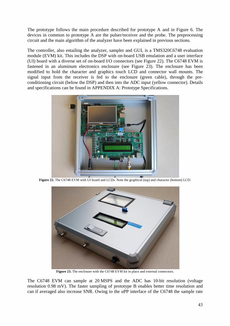
43
The prototype follows the main procedure described for prototype A and in Figure 6. The
devices in common to prototype A are the pulser/receiver and the probe. The preprocessing
circuit and the main algorithm of the analyzer have been explained in previous sections.
The controller, also entailing the analyzer, sampler and GUI, is a TMS320C6748 evaluation
module (EVM) kit. This includes the DSP with on-board USB emulation and a user interface
(UI) board with a diverse set of on-board I/O connectors (see Figure 22). The C6748 EVM is
fastened in an aluminum electronics enclosure (see Figure 23). The enclosure has been
modified to hold the character and graphics touch LCD and connector wall mounts. The
signal input from the receiver is fed to the enclosure (green cable), through the pre-
conditioning circuit (below the DSP) and then into the ADC input (yellow connector). Details
and specifications can be found in APPENDIX A: Prototype Specifications.
Figure 22. The C6748 EVM with UI board and LCDs. Note the graphical (top) and character (bottom) LCD.
Figure 23. The enclosure with the C6748 EVM kit in place and external connectors.
The C6748 EVM can sample at 20 MSPS and the ADC has 10-bit resolution (voltage
resolution 0.98 mV). The faster sampling of prototype B enables better time resolution and
can if averaged also increase SNR. Owing to the uPP interface of the C6748 the sample rate

44
of 20 MSPS is currently limited by the ADC module alone, and no discontinuities can be seen
as with prototype A.
5.4.2.2 Software
The software solution (the main code is found in APPENDIX E: Source Code) can be used in
two different modes, clinical and debug. The main differences between these are that the GUI
displays different amounts of information and that the reference distance differs. In clinical
mode, an average of a number of distances is taken as a reference distance on initialization,
while the last iteration distance is used in debug mode. The steps of the program can be seen
in Figure 24.
Figure 24. An overview of the prototype software. In addition to the differences between modes seen in the flowchart, the
GUI is different in the way it displays warnings and gives user feedback.
The remainder of this section will illustrate the steps of Figure 24 for a signal taken during
clinical testing. This signal should not be considered the best possible. It constitutes a
common signal during tests with a handheld probe and has been chosen to illustrate the
algorithm and also to highlight the difficulties in this application.
The program begins with the ADC and trigger GPIO being set up and used to collect
2048 sampling points from the signal sent by the receiver. After sampling, the signal is
normalized so that the waveform is centered around zero. This is needed for the next step in
Start
Clinical mode?Compute mean
starting distanceYes
Sample signal
(2048 points)
No
Wavelet
filtering
Remove soft
tissue echoes
Echo exists?
TGC processing
Yes
Enveloping via
the Hilbert
Transform
Set warning =
NO_ECHONo
Peak detection
Competing
echoes?
Calculate
distance for
highest peak
No
Clinical or
echo last loop?
Movement
detected?
Yes
Periodic data
save?
No
Show warning
and motions if
any on LCD
No
Save data to SD
cardYes
Set warning = COMPETING_
ECHOES
Yes
Unrealistic
movement?Yes
Set warning = UNREALISTIC_
MOVEMENT
Yes
Set warning =
MOVEMENTNoNo

45
the signal processing to work properly, which is denoising with the wavelet transform. An
example of a sampled signal can be seen in Figure 25.
Figure 25. A non-processed signal consisting of 2048 sampling points sampled at 20 MSPS. Parts of the signal are outside
the y-axis limits in this figure.
The denoising is performed, as described in 5.3.1.1, by calculating the wavelet transform of
the signal using the mother wavelet Symlet4, followed by a calculation of the MAD standard
deviation used to obtain soft threshold coefficients. Lastly, the coefficients are inverse
transformed, resulting in a denoised signal. Figure 26 illustrates the denoised version of the
signal in Figure 25.

46
Figure 26. The waveform obtained by denoising the sampled signal with the Wavelet Transform.
When the signal has been denoised, the echoes given by layers of soft tissues preceding the
bone has to be removed. This is achieved by traversing through the signal until a given
number of indexes in a row have values below a given threshold. When this index is
encountered, all of the foregoing points are set to zero. The choice of the parameters (number
of indexes and threshold) is a trade-off between the certainty of soft tissue echoes removal
and the certainty in retaining small distance bone echoes. This functionality is implemented
with the assumption that there is a somewhat homogenous volume between layers of soft
tissue and bone.
The next step in the procedure is to make certain that an echo exists, which is accomplished
by examining the denoised signal in the frequency domain (see Figure 27). If the values for a
given number of indexes in a row, within a given frequency range, is larger than a given
threshold, the presence of an echo is ensured. Because the signal may differ in frequency
content due to signal quality, the frequency range must be of a sufficient size. If an echo is not
present, the distance is set to zero and a warning is set.

47
Figure 27. The frequency spectrum of the denoised signal.
To find similarities with the clean US signal originating from the transducer, Figure 27 may
be compared to Figure 10. A signal with distorted, low amplitude, or no echo does not have
the underlying shape found in these figures.
If an echo exists, TGC is performed according to Eq. 4. Some receivers use logarithmic
compression of the signal in order to account for large variations, which would require linear
attenuation compensation in the final signal. However, the DPR300 is linear, enabling the use
of Eq. 4. As stated in [14], TGC is commonly performed within the electronics of the receiver.
Low level noise present in the far end of the signal will be highly amplified when applied in
software. Therefore a user factor has been added as a parameter to control the amount of
compensation to a trade-off point between amplitude compensation and noise.
TGC is followed by an enveloping of the denoised signal using the analytic signal. The result
of such enveloping can be seen in Figure 28.

48
Figure 28. The result of enveloping the denoised and time gain compensated signal.
Peak detection is then performed to find the highest peaks in the processed signal. The result
is used to analyze whether the signal contains competing peaks. This is an important function
because the echo is ultimately defined as the highest peak.
From this point on, the prototype has found a distance and must now compare the current
distance to either the previous distance (debug mode) or the starting distance (clinical mode)
and perform a plausibility check. If the last measurement in debug mode had no echo, there is
no comparison. If movement is detected, the software confirms that this is a reasonable
movement. An unreasonable movement occurs if the distance has changed faster than what is
considered possible in a clinical setting. This error occurs if the threshold for competing peaks
is set incorrectly, thus enabling a competing peak to drastically change the distance for the
next iteration.
Finally, the distance buffer is stored on a SD card if full and relevant information (depending
on mode) is written to the LCD.

49
6. RESULTS
Verification of the prototype was done using the tests in APPENDIX B: Test Protocol.
Additional weight was laid on clinical tests. Calibration was made before the tests with a
negative zero offset term to account for electrical and mechanical delays. This delay can
partly be seen in the signals obtained from the system by investigating the position of the
transmitted pulse.
The result for test 1 has been combined with the test result of prototype A and can be seen in
Table 6.
Table 6. The total test results for test 1.
Measured values [mm]
Prototype A Prototype B
Distance [mm] Mean ± STD Error Mean ± STD Error
5.0 5.9 ± 0.1 +0.9 5.0 ± 0.02 +0.0
10.0 10.8 ± 0.1 +0.8 10.0 ± 0.01 +0.0
15.0 15.6 ± 0.1 +0.6 15.0 ± 0.01 +0.0
20.0 20.5 ± 0.1 +0.5 20.0 ± 0.02 +0.0
25.0 25.3 ± 0.1 +0.3 25.1 ± 0.01 +0.1
30.0 30.2 ± 0.1 +0.2 30.1 ± 0.02 +0.1
35.0 35.1 ± 0.1 +0.1 35.1 ± 0.01 +0.1
40.0 39.9 ± 0.1 -0.1 40.1 ± 0.02 +0.1
45.0 44.8 ± 0.1 -0.2 45.1 ± 0.01 +0.1
50.0 49.6 ± 0.1 -0.4 50.1 ± 0.02 +0.1
55.0 54.4 ± 0.1 -0.6 55.1 ± 0.02 +0.1
60.0 59.3 ± 0.1 -0.7 60.2 ± 0.01 +0.2
The mean update frequency during test 1 was 2.0 Hz (which also becomes the PRF for the
system). There was no experimentally visible correlation with gain or signal amplitude.
Further details regarding execution time distribution can be found in Figure 29.

50
Figure 29. The proportions of execution times for different parts of the program.
Test 2 gave a measured distance difference of 15.0 mm with an equal STD of 0.02 mm for the
two distances.
Clinical tests were focused on the logic of the prototype. The prototype was found to have
exceptionally few false positives, i.e. the prototype did not falsely indicate movement if no
echo was seen on the oscilloscope. False negatives however were common during handheld
tests. Nevertheless, the parameters currently set were deemed appropriate due to the fact that
the prototype should have a margin to avoid sudden signal loss or unsteady measurements.
Prototype B could steadily find echoes from the signals obtained using the neck rest, in
contrast to prototype A.
1%
77%
4%
2%
9%
1% 3% 3%
Execution Time Distribution
Signal sampling
Wavelet denoising
Echo existence checking
Time gain compensation
Enveloping
Finding peaks
Writing distances to file
Other

51
7. DISCUSSION
7.1 Solution Drawbacks The implementation of the logic algorithms was performed, as mentioned in 5.3.1.2, by brain-
storming solutions and experimenting with them. The advantage of such an approach is that
the implementation becomes customized for the application at hand and can give a more
robust solution. However, not having a literature study to fall back on can, during
development, be seen as an uncertainty in whether or not a solution might hold. The amount
of logic introduced in the system was kept low since more logic can lead to less clarity for the
user in how the system operates. Such a separation between the user and the real result can
lead to misinterpretation of the result.
One main issue to decide before developing logic algorithms was how to manually separate
the information found in the signal. More precisely, how the bone echo is identified. To gain
experience with the actual distance from different angles, a B-mode US was taken on the
authors. Furthermore, due to the large reflection and attenuation of bone, bone should result in
shadowing. Variations however may occur due to artifacts.
When a signal contains several of these echoes (also possibly due to artifacts) it is extremely
difficult to distinguish their origins, i.e. which echo represents the reflection from what
interface. The reason is that the denoising of the signal does not differentiate echoes due to
identical frequency content. In addition, in the case of the neck, there is no proper way of
making a distinction between bone and soft tissue echoes merely by echo shape. However, a
separation can be made if an assumption that there is a minimum distance between the echoes
is made, since soft tissue echoes in the beginning of the signal are adjoining. Such an
assumption was supported experimentally during the project, in which the prominent layers of
soft tissue were compressed when pressure was applied to the probe, but in a logical way
changed the distance to the largest echo further in.
The algorithm to detect where soft tissue ends is described in section 5.4.2.2. The value for
the minimum distance parameter was not calculated based on true anatomy, but
experimentally chosen. However, anatomy was the foundation for understanding how to
manually identify the echoes. The algorithm handles the variation in depth of the soft tissues,
which is correlated with the size of the neck and the pressure with which the probe is pressed
against it, as long as the minimum distance between soft tissue layers and bone is preserved.
This approach is favored in clinical situations since the amount of soft tissue around the spine
may differ from one patient to another.
To perform the envelope of a signal to obtain a smooth outlining of the extremes works well
with ideal signals as in Figure 8. However, on a real signal, where some noise exists and
where the echo has a deviating shape, the process may fail. This can be seen in Figure 29 in
which parts other than just the echo are also enveloped. Sometimes the enveloping process
also has a tendency to result in more than one extreme around the echo, which can lead to
uncertainties in choosing one point that should represent the echo. However, the process is
more robust than just taking the extreme value directly from the denoised signal.
The hardware aim to amplify the echo to maximum size relating to the ADC input in clinical
tests proved to be difficult. With ideal components the design would perform this very task.
However, the maximum level of clipping of the diodes and the limitation in amplification due

52
to ADC tolerances appeared to restrict the result of the design to lower levels of echo
amplitude. The maximum initial voltage of the echo was furthermore not known. To identify
this, the signals obtained with a new neck rest are required. Receiver settings is another factor
influencing the initial voltage and therefore also the parameters used in circuit design.
7.2 System Errors One source of error may be the zero offset used when calculating the distance. The offset is
needed due to both electrical and mechanical delays that increase the time between the
triggering and the sampling of the signal, in conjunction with the system specific definition of
where an echo begins and ends. The offset was calibrated at a distance of 15 mm with the
setup in test 1.
However, a seemingly linear change in the error of measurements was seen during the test for
increasing distance (see Table 6), which implies a correlation between error and change in
distance. This can have to do with uncertainties in the test rig, the placement of the probe, or
the prototypes themselves. For example, as seen in Figure 14, the shape of the echo changes
for larger angles. It was also found during experiments that the shape changes for increasing
distances if the probe is slightly angled. This could be part of the minor increasing error seen
with prototype B. However, since the interval in which distances are compared for realistic
movements is short, the spread in Prototype B becomes less significant. The larger error seen
for prototype A mainly depends on the factor multiplied with the distance result in the
software. If calibration is performed with a straight line (y = kx + m) instead of only a factor,
this visible error is removed. However, the zero offset term, corresponding to m, is larger in
prototype A, indicating a difference in delay for both systems. Because the source of the
linear error, corresponding to k, may be due to the test rig, and the error is small for the
relevant distance comparisons, no correction has been made for prototype B.
The angle is also a vital part of the setup for finding a strong bone echo signal. Even though
miniature angles and scatter are inevitable due to the rough surfaces on bone, care must be
taken to align the probe. The exact anatomy of individuals, and therefore the flat surfaces of
the vertebrae, is however hard to find. Therefore, an adequate neck rest with the ability to
adjust the probe for each individual is needed. The lack of such a neck rest has made clinical
tests more difficult. No tests measuring movement over long periods, such as the time for a
RT treatment, have been performed. Additionally, the accuracy and precision during clinical
setup is not known.
7.3 Development Compromises An important aspect relating to the logics of the final program was to avoid false negatives,
meaning that the prototype falsely interprets no movement. Due to the trade-off with false
positives, this would mean increased warnings from the system. The implementation of logics
and warnings adds complexity to the system, but this is necessary in order to deal with the
problems of prototype A. The ability to analyze measurements is based on the parameters
given to the system. Perhaps the most important is the threshold for checking if there is an
echo in the signal. If set too low, the system will believe that there is a good signal and
inevitably introduce false readings. If it is set too high, the system will be too complicated to
setup. This must be thoroughly tested in a simulated RT situation. The different situations that
can occur can be seen from the test results, in which the STD (indicating signal quality) is

53
almost doubled for measurements on the spine phantom compared to measurements on a flat
surface. The threshold must be set for the specific neck rest and patient setup at hand.
As can be imagined from 4.2 there is a continuous flow of patients in the RT unit. This
highlights another trade-off related to the previously mentioned compromise, namely that of
setup time versus acquiring a good signal. To be useful, the system must be able to setup
easily. Even though it accurately measures movement it can be discarded due to financial
reasons. Referring to other IFMM systems, this solution requires a connection between probe
and patient. This can be seen as an inconvenience compared to IR and x-ray systems. Again, a
great deal depends on the neck rest.
When running the program for Prototype B in clinical mode, it is important to make sure that
a suitable reference distance is used during the whole procedure. The choice is a crucial
element in obtaining accurate and reliable measurements. The reference distance is computed
in the beginning of the program by performing measurements until ten distances in a row are
acquired without any error messages. The average of those is chosen as the reference distance.
If any errors are obtained, a message to adjust the probe is displayed so that a better probe
placement can be achieved. The selection of the number of distances in a row that have to be
error free is a trade-off between the precision of the reference distance and the risk of having
movements during the reference distance calculation. In this case, ten distances were chosen
because it gave satisfactory results during experiments.
During tests it is preferable to obtain signals with the highest possible quality. This can be
achieved by reducing gain, which helps reduce the noise level in the signal and decrease the
amount of interfering echoes. However, such a reduction can lead to difficulties in finding an
echo in the signal due to the decrease in amplitude the reduction leads to. The choice of gain
is therefore a trade-off between signal quality and difficulty in finding an echo. This can be
seen in test 1 and test 2, where the STD is doubled for the correct spine geometry. Gain was
chosen individually for the two prototypes for each test according to the described trade-off.
In general, prototype B required less gain for good quality signals.

54

55
8. CONCLUSIONS
The prototype developed is functional and fulfills the aims of this project. It can accurately
measure the distance to the spine and display this on a GUI, which enables movement
detection. The software is precise and robust, and the hardware has improved signal
acquisition and prototype enclosing. Even though no statistical tests were performed, the
visible difference in precision and accuracy found in test 1 and test 2 shows that prototype B
is a major improvement.
All of the original prototype limitations mentioned in 5.1.4 have been accounted for. Some
have however been shown to be difficult to avoid and therefore warnings have been
implemented in the system.
This prototype constitutes a non-invasive IFMM system capable of detecting movements with
sub millimeter accuracy. It uses no ionizing radiation and runs in real-time with direct
measurements on the cervical spine. The prototype is ready for clinical tests in a hospital
environment when a neck rest with sufficient ability to adjust the probe has been integrated
with the system.

56

57
9. FUTURE WORK
Further desirable development following this prototype can be summarized with the following
points.
More probes should be added to the system in order to detect movements in three
dimensions. The probes could be aimed at a number of vertebrae in different angles. A
probe redundancy can also be applied to diminish the problem of lost signals. The
components that are required for the expansion of the prototype to handle several
probes can be divided into two parts. First, a number of GPIO pins are needed, for
example, the J13 or J30 pins of the expansion boards on the C6748 EVM baseboard.
Second, a multiplexer (a device to handle several analog signals) is required to
correlate different GPIO pins with different probes. The probes would be connected to
the multiplexer, which only passes signals from a specific probe if the associated
GPIO is set to high by the controller. A small code fragment could be written in the
main function of the prototype to coordinate and control the activation and
deactivation of the probes by setting the GPIO pins to relevant states. Running the
current program for all of the probes, one at the time, can then give information about
movements in three dimensions.
A new neck rest must be developed in order to enable robust fixation of the probe.
Possible angles should be investigated in order to position appropriate holes in the
neck rest. However, by simply copying the aim of the current neck rest would give
two adequate angles aimed at the right and left lamina of the vertebra. Probe
adjustments must be possible when the patient is in a supine position and with low
time consumption. Ideally, three degrees of translational freedom in addition to two
degrees of rotational degrees should be possible for every probe. Ergonomics must
also be considered. The best signal is acquired in a less ergonomically suited position
of the head in the current neck rest. If the prototype is to be a success, the patient must
not be too uncomfortable.
With a new neck rest the prototype can be more thoroughly tested on a subject in the
supine position with body fixation (e.g. the Elekta bluebag). Clinical tests during
radiation treatments follows.
The GUI can be expanded to also include the graphics touch LCD. Preparations have
been made in the form of a LCD window in the enclosure and example programs of
how the LCD can be used. One alternative is to show the full signal on the LCD,
similar to an oscilloscope, and to enable user touch interaction such as pause and stop
options.
In a future release, the calculated movements could also be coupled to IFMM tracking
systems, in which the patient couch could be moved in response to spine and tumor
movements. In contrast to gating procedures where the radiation is halted, this would
reduce treatment time.
The prototype can also be expanded to include other parts of the spine, for instance to
the thoracic region of the spine, if the prototype is successful in determining patient
motion during treatments. An entire couch must then be designed where the extra

58
probes can be attached and at the same time have contact with the skin. This may be
difficult with today’s customary body fixation mattresses that surround the patient.

59
REFERENCES
[1] E. AB, "Elekta Annual Report," 2012. [Online]. Available:
http://www.elekta.com/dms/elekta/elekta-assets/Investors/pdf/ELE_ar-11-
12_ENG/Elekta_AR11-12_ENG.pdf. [Accessed 30 1 2012].
[2] H. Gray, Anatomy of the Human Body, Philadelphia: Lea & Febiger, 1918; Barteby.com,
2000. [Online]. Available: http://www.barteby.com/107/. [Accessed 24 1 2013].
[3] editor E. B. Podgorsak and sponsored by IAEA, Radiation Oncology Physics: A
Handbook for Teachers and Students, Vienna: International Atomic Energy Agency,
2005.
[4] S. H. Levitt, J. A. Purdy, C. A. Perez and P. Poortmans, Technical Basis of Radiation
Therapy Practical Clinical Applications, Berlin: Springer-Verlag, 2012.
[5] AAPM (the American Association of Physicists in Medicine) Task Group
101, ”Stereotactic body radiation therapy: The report of the AAPM Task Group 101,”
Medical Physics, vol. 37, nr 8, pp. 4078-4101, 2010.
[6] A. Sahgal, "Current state of brain and spine radiosurgery and future applications," Future
Medicine, vol. 2, no. 1, pp. 17-22, 2013.
[7] T. L. Stedman, Stedman's Medical Dictionary, Baltimore: Williams & Wilkins, 1990.
[8] N. Agazaryan, S. E. Tenn, A. A. Desalles and M. T. Selch, "Image-guided radiosurgery
for spinal tumors: methods accuracy and patient intrafraction motion," Physics in
Medicine and Biology, vol. 2008, no. 53, pp. 1715-1727, 2008.
[9] A. Martin and G. A, "Stereotactic Body Radiotherapy: A Review," Clinical Oncology,
vol. 22, no. 3, pp. 157-172, 2010.
[10] R. Åslund, Interviewee, Director Strategic Portfolio Management, Elekta Instrument AB.
[Interview]. 15 February 2013.
[11] W. A. Hall, L. J. Stapleford, C. G. Hadjipanayis, W. J. Curran, I. Crocker and H.-K. G.
Shu, "Stereotactic Body Radiosurgery for Spinal Metastatic Disease: An Evidence-Based
Review," International Journal of Surgical Oncology, vol. 2011, Article ID 979214,
2011.
[12] W. R. Hendee and R. E. Russell, Medical Imaging Physics, Fourth ed., New York: John
Wiley & Sons, Inc., 2002, pp. 303-353.
[13] P. Allisy-Roberts and J. Williams, Farr's Physics for Medical Imaging, Second ed.,
Philadelphia: Saunders Elsevier, 2008, pp. 147-168.

60
[14] J. T. Bushberg, J. A. Seibert, E. M. Leidholdt jr and J. M. Boone, THE ESSENTIAL
PHYSICS OF MEDICAL IMAGING, Philadelphia: Lippincott Williams & Wilkins,
2002, pp. 469-555.
[15] B. Jacobson, Jacobsons Medicin och Teknik, Fifth ed., Lund: Studentlitteratur, 2006, pp.
344-356.
[16] J. Luckner and B. Hibbard, Interviewees, Technical Representative and Chief Marketing
Officer, Imaginant Inc (previously JSR Ultrasonics Inc). [Interview]. 2 February 2013.
[17] K. A. Fowler, G. M. Elfbaum, K. A. Smith and T. J. Nelligan, "THEORY AND
APPLICATION OF PRECISION ULTRASONIC THICKNESS GAGING," Insight –
Non-Destructive Testing and Condition Monitoring , vol. 2, no. 10, 1997.
[18] K. V. Shibu, Introduction to EMBEDDED SYSTEMS, New Delhi: Tata McGraw Hill
Education Private Limited, 2009.
[19] R. C. Gonzales and R. E. Woods, Digital Image Processing, New Jersey: Pearson
Education, Inc, 2008.
[20] C. R. Johnson Jr, W. A. Sethares and A. G. Klein, Software Receiver Design: Build Your
Own Digital Communication System in Five Easy Steps, Cambridge: Cambridge
University Press, 2011.
[21] Texas Instruments, "High-Speed, Analog-to-Digital Converter Basics," 2011. [Online].
Available: http://www.ti.com/lit/an/slaa510/slaa510.pdf. [Accessed 4 3 2013].
[22] P. Daponte, G. Fazio and A. Molinaro, "Detection of Echoes Using Time-Frequency
Analysis Techniques," IEEE Transactions on Instrumentation and Measurement, vol. 45,
no. 1, pp. 30-39, 1996.
[23] R. Chassaing, Digital Signal Processing and Applications with the C6713 and C6416
DSK, New Jersey: John Wiley & Sons, 2005.
[24] Y. Ruqiang and R. X. Gao, Wavelets: Theory and Applications for Manufacturing, New
York: Springer, 2011.
[25] R. L. Allen and W. D. Mills, Signal Analysis: Time, Frequency, Scale, and Structure,
New Jersey: John Wiley & Sons, 2004.
[26] L. S. John, Biosignal and Biomedical Image Processing: MATLAB-Based Applications,
New York: Marcel Dekker, 2005.
[27] L. Debnath, Wavelet transforms and their applications, Boston: Birkhäuser, 2002.
[28] Y. Zhao, L. E. Atlas and R. J. Marks, "The Use of Cone-Shaped Kernals for Generalized
Time-Frequency Representations of Nonstationary Signals," IEEE Transactions on
Acoustic, Speech, and Signal Processing, vol. 38, no. 7, pp. 1084-1091, 1990.

61
[29] H.-G. Stark, Wavelets and Signal Processing: An Application-Based Introduction,
Berlin: Springe-Verlag, 2005.
[30] A. Abbate, J. Koay, J. Frankel, S. C. Schroeder and P. Das, "Signal Detection and Noise
Suppression Using a Wavelet Transform Signal Processor: Application to Ultrasonic
Flaw Detection," IEEE Transactions on Ultrasonic, Ferroelectrics, and Frequency
Control, vol. 44, no. 1, pp. 14-26, 1997.
[31] J. C. Goswami and A. K. Chan, Fundamentals of Wavelets: Theory, Algorithms, and
Applications, New Jersey: John Wiley & Sons, Inc., 2011.
[32] A. T. Walden and D. B. Percival, Wavelet Methods for Time Series Analysis, New York:
Cambridge University Press, 2000.
[33] L. Råde and B. Westergren, Mathematics Handbook for Science and Engineering, Lund:
Studentlitteratur, 2004.
[34] E. Oruklu, Y. Lu and J. Saniie, "Hilbert Transform Pitfalls and Solutions for Ultrasonic
NDE Applications," in IEEE International Ultrasonics Symposium Proceedings,
Chicago, 2009.
[35] R. K. Rao Yarlagadda, Analog and Digital Signals and Systems, New York: Springer,
2010.

62

63
APPENDIX A: Prototype Specifications
This appendix features selected specifications for the different components of the prototypes.
The pulser/receiver and probe are the same for both prototype A and B. The data have been
taken from user manuals and technical documents pertaining to the device at hand.
A selection of the controller, sampler and analyzer specifications (including DSP and
daughter boards) can be seen in Table 7.
Table 7. Selected specifications for the controller, analyzer and sampler. Note that the ADC and NAND flash for prototype B
is situated on the user interface board of the C6748 EVM kit and not on-chip of the C6748 DSP.
Prototype A Prototype B
Model TI TMS320F28335 TI TMS320C6748
CPU C28x (32-Bit) C674x (32-Bit)
RAM 68 KB 320 KB + 128 MB mDDR
Flash 512 KB 8 MB NOR + 512 MB NAND
Clock Frequency 150 MHz 456 MHz
ADC 12-Bit, 12.5 MSPS1 10-Bit, 20 MSPS
1
Other 88 GPIO pins
uPP, SD card slot, 2 LCDs, DIP
switches, real-time clock,
available with ARM processor
1MSPS – mega samples per second
In Table 8 and Table 9 follows the pulser/receiver specifications and settings used.

64
Table 8. Selected specifications for the pulser/receiver.
Model JSR Ultrasonics DPR300
Pulse Type Negative spike pulse
Pulse Duration 10-70 ns FWHM1 for 50 load
Mode Pulse-echo or through transmission
Gain -13 to 66 dB (1 dB steps)
High Pass Filter 1 – 12.5 MHz (5 steps)
Low Pass Filter 3 – 35 MHz (6 steps)
Pulse Repetition Rate 100 – 5 KHz for internal; 0 – 5 KHz for external
Pulse Amplitude 100 – 900 V (16 steps)
Pulse Energy High (4 steps); Low (4 steps)
Damping Damping settings (16 steps)
External Trigger Input 3 – 5 V
Input Impedance 500
Output Impedance 50 1FWHM – Full width half maximum
Table 9. The settings commonly used during testing.
Receiver Echo
Relative gain 35 dB
HP filter 2.5 MHz
LP filter 7.5 MHz
Trigger External
Pulse amplitude 16
Pulse energy Low 4
Damping 16
The specifications for the probe can be seen in Table 10.

65
Table 10. Selected specifications for the probe.
Manufacturer Precision Acoustics Ltd
Model PA391
Transducer Type Unfocussed PVdF
Nominal Centre Frequency 5.00 MHz
Transducer Diameter 9 mm
Outline Dimensions 3420 mm (length, diameter)
In Table 10, PVdf refers to the material used to achieve the piezoelectric effect. A
piezoelectric crystal is often used in today’s transducers. However, there are also polymers
with piezoelectric ability, as with the PVdF polymer. The connections between the equipment
used can be seen in Table 11.
Table 11. The ports connected between different modules of the system. The abbreviation m/m stands for male/male. All
BNC cables are male/male.
Connection Port labels Cable type
Enclosure → Pulser/receiver Input → Receiver output BNC
Enclosure → Pulser/receiver Trigger → Trig/sync BNC
Enclosure → Computer Emulation → USB port USB (m/m)
Enclosure → Power adapter 5V Power → 5V 3.8A AC adapter Power cord
Pulser/receiver → Transducer T/R → No label BNC

66
APPENDIX B: Test Protocol
Test Setup All non-clinical tests in this report have been done with a test rig specifically developed
during this project for testing the prototypes. The test rig consists of an L-shaped steel stance
with a downwards vertically directed linear motion guide actuator. The actuator used is a
100 mm stroke THK KR20A with a positioning accuracy of below ±0.1 mm (defined as the
maximum of the deviations from the true traveled distances through the whole stroke range)
and positioning repeatability of ±0.01 mm. Attached to the actuator is a mount for the probe.
The probe is put in place using mounting putty and cable ties in order to enable final angle
adjustments. Care was taken to avoid air bubbles on the target and transducer. To account for
errors in the setup, the published data have been created simultaneously for prototype A and B.
Prototype A was however tested separately in the beginning of the project in order to find its
properties. The test rig can be seen in Figure 30.
Figure 30. The test rig used during tests. Observe that for all tests the probe was further fixated with cable ties.
Clinical tests have been performed with a preliminary neck rest prototype developed for
prototype A. The neck rest have been attached to a couch (Figure 31). There has been no
probe fixation other than the angle created by the holes in the neck rest and fixation by hand.
Two angles to the neck have shown to be adequate. The first is aimed at the vertebra body
through the posterior triangle. This angle is not supported by the neck rest. The second angle,

67
obtained with the current neck rest and used in these tests, is through the trapezius muscle to
the lamina.
Figure 31. The test subject setup used for clinical tests using the existing neck rest without probe fixation.
Tests A test protocol was written to standardize testing of the prototypes to enable comparisons and
areas of improvements. These can be found in the following section. For all tests, gain was
adjusted in order to optimize the signal for the specific prototype.
Test 1 – Ideal Conditions
The prototype is to be tested during ideal conditions in order to examine accuracy and
precision of absolute distance measurement alone (see setup in Figure 30). Hence, the test
may also be performed to calibrate the prototype. These ideal conditions involve a water tank,
a standing block target of carbon fiber (8.8 2.5 3.5 cm), and the test rig including the probe.
The block is designed to avoid in-material reverberations with its height. Additionally, the
acoustic properties (impedance, attenuation etc.) have been found adequate by an
experimental approach. The target is immersed into the water tank. The probe will be lowered
to physically connect to the target. This position is considered to be distance 0. After this
calibration, the distance to the target is equal to the upwards movement of the actuator.
Measurements will be taken at discrete distances. Distances will be from 5.0 mm to 60.0 mm
in steps of 5 mm. For every distance, 1000 measurements will be taken. Mean and STD
values will be calculated.
Test 2 – Spine Phantom
This test will be done on a geometrically correct spine phantom in order to test the prototypes
on less ideal signals but with maintained control of experiment variables (internal validity).
The test rig is the same as in test 1. Due to the difficulty of finding the distances to the exact
point on the phantom, this test will focus on difference in distances alone. The phantom will
be placed below the probe and the probe lowered to a distance of more than 5 mm to the
phantom. After 1000 measurements have been made, another distance 15.0 mm above this
point will be measured. The mean from each distance will then be subtracted with the mean of

68
the neighboring point of measurement. The difference can be compared to the actual
movement of the actuator. STDs will also be taken for each measurement in order to permit
approximate comparisons to test 1.
Test 3 – Angle Tolerances
The importance of accurate positioning of the probe in respect to the target will be tested by
observing the signal in ideal conditions while changing the angle of the test rig, thus
consequently also the probe. This can also be seen as simulation of an irregular surface. To
acquire accurate angle readings, the test rig will be touted, independently of the horizontal
water tank. Thus, the axis of rotation will not go through the probe but the side of the test rig,
introducing an increase in distance between the probe and the target for higher angles.
However, this will not affect the ability to draw conclusions regarding the changes in echo
shape. The oscilloscope signal will be observed for several angles in increments of 1.0°.
Test 4 - Clinical Tests
Tests with higher external validity should also be conducted in order to find how the
prototypes perform in real-world situations. In this work, a qualitative investigation is
adequate on only a few subjects. In these tests, the probe should be handheld to the neck,
changing the position and angle of the probe to find a signal with the aid of an oscilloscope. A
handheld probe could introduce errors, but the robustness and overall behavior of the
prototypes should regardless be observable. To obtain some reproducibility, the neck rest
should be used.

69
APPENDIX C: Circuit Calculations
The circuit was designed so that the input signal would be cut at a proper level, filtered and
then amplified so that the echo would be represented by a large portion of the ADC. The
choice of different components and calculations are described below.
Diodes As seen in Figure 17, the circuit consists of two identical schottky diodes placed in parallel
with opposed anodes/cathodes to clip the signal equally for positive and negative voltages. As
described in 1, the goal was to clip most of the transmitted signal while preserving the
amplitude of the echo. Therefore a diode with proper forward current and voltage was chosen,
more precisely, the Schottky barrier diode BAT85. The BAT85 has a low forward voltage and
is made for ultra high-speed switching applications. The amplitude after clipping in the final
circuit has been shown to be maximum 550 mV for the receiver settings generating the largest
amplitude signal.
Filters To filter out frequencies above and below the most prominent in Figure 10, RC filters of first
order were designed. Given the circuit in Figure 17 the cutoff frequencies and phase shift for
the low- and high-pass filters can be calculated as follows:
1. The part of the circuit to the right and in parallel with C2 can be omitted due to the
input impedance of the operational amplifier being considerably larger than C2.
2. The cutoff frequency for the low-pass filter is given by the components R4 and C2 and
is equal to:
MHz4.20242
1
CRfcL
3. The high-pass filter is given by the capacitor C1 and resulting impedance of R2, R3,
R4 and C2. The power supply is treated as a short circuit and the diodes as a circuit
break for the signal of interest, i.e. when the diodes do not conduct. At 5MHz, the
resulting impedance, R', equals:
6152||3||
21052
14'
6RR
CRR
And the cutoff frequency equals:
MHz73.11'2
1
CRfcH
4. The cutoff frequency for the high-pass filter differs depending on the frequency of the
signal since the impedance of C2 is frequency dependent. If the frequency goes to zero,

70
the cutoff frequency is 1.2MHz, while if it goes towards infinity, the cutoff frequency
goes towards 3.9MHz.
5. The phase shift of the two filters is given by:
cHcLf
f
f
f0101 tan90tan
Thus the phase shift at 5 MHz is -5°.
The diagram of the transmission for the designed filters can be seen in Figure 32. The part of
the frequency spectrum that gives highest transmission coincides sufficiently with the
frequency spectrum of the ultrasound beam in Figure 10.
Figure 32. A bode plot of the magnitude of the signal through the RC filters for different frequencies.
Amplifier The operational amplifier in the circuit was chosen after its ability to fulfill the following
demands:
Can be driven by a 3.3V single supply.
Can handle a 10 MHz signal without distortion or significant attenuation.
Has rail-to-rail output.
To avoid distortion, the required slew rate (SR) for a 10 MHz signal with 2.3 Vp-p is
721010215.1 6 SR V/µs according to the maximum derivative of a sine signal. To

71
avoid attenuation, a theoretical 0.1 dB bandwidth of minimum 10 MHz was decided for a gain
of 8. The resulting operational amplifier, LMH6612, has according to the datasheet a slew rate
of 330 V/µs for a 2 V step and a 0.1 dB bandwidth at 47 MHz for a gain of 2.
Amplification was made with a non-inverting amplifier circuit, entailing resistors R5 and R6.
To obtain a final signal of maximum 1.15 V, an amplification of 28.292.0550.015.1
was required, where the factor 0.92 is due to the attenuation by the filters at 5 MHz. Resistors
2.15R kΩ and 5.16R kΩ gives an amplification of
25.25
65
R
RRA
v.
When using single supply a higher DC level is needed to conform to the input voltage range
of the amplifier (-0.2 - 1.8 V). A voltage divider was created to match to these demands
consisting of resistors R2 and R3 (see Figure 17). The values 8.2 Ω and 1 Ω were chosen,
with a theoretical new DC level of 36012.813300 mV in isolation and for a 3.3 V
supply. This gives a margin of 5020092.0550360 mV from the maximum amplitude
receiver signal to the lower input voltage of the amplifier. When connected to the other
components of the circuit the DC level is higher and therefore satisfactory.

72
APPENDIX D: Evaluated Algorithms
In this appendix, algorithms that can be used for signal processing of ultrasound signals are
tabled in Table 12. The algorithms were divided into two groups, time domain and time-
frequency analysis methods. The algorithms marked with green were considered to have the
highest potential and were implemented in MATLAB.
Table 12. Signal processing algorithms that can be used for echo detection.
Time-frequency analysis methods
Cepstrum Transform
Chirplet Transform
Cross-Ambiguity Function
Fundamental Frequency Estimation
Fractional Fourier Transform
Gabor Transform Prototype 1b
Genetic Algorithm Optimized Matching Pursuit
Hilbert Transform Used in all Prototypes
Short-Time Fourier Transform Prototype 1a
Split Spectrum Processing
Wavelet Transform Prototype 4a
Wavelet Packets Prototype 4b
Wigner-Ville Distribution Prototype 2
Zhao-Atlas-Marks Distribution Prototype 3
Time domain analysis methods
Finding Zero Crossings
Model-Based Detection
Model-Based Estimation
Probability Density Function
Runtime Filters
Sliding Standard-Deviation Window Can be used in Prototypes
4a and 4b

73
APPENDIX E: Source Code
The code for the final software solution was written in C/C++ and was divided into different
modules. The program has a total .out file size of 180 kB. Program data is mapped at 240 kB
in the linker command file. Since the number of lines in the whole source code (including
external libraries) exceeds 10 000, it is not feasible to include all of it in this appendix.
However, a fragment of the source code will be provided. The cpp file of both the main
function and the helping class that coordinates the execution of the program can be found
below. Some comments are removed from the original source code to avoid line wrapping and
ease the readability in this appendix.
Main.cpp
extern "C"
#include "BSL_inc/types.h"
#include "BSL_inc/evmc6748.h"
#include "BSL_inc/evmc6748_timer.h"
#include "BSL_inc/evmc6748_i2c_gpio.h"
#include "BSL_inc/evmc6748_i2c.h"
#include "BSL_inc/evmc6748_gpio.h"
#include "BSL_inc/evmc6748_led.h"
#include "BSL_inc/evmc6748_sysconfig.h"
#include "BSL_inc/write_lcd_char.h"
#include "BSL_inc/evmc6748_mmcsd.h"
#include "BSL_inc/evmc6748_rtc.h"
#include "BSL_inc/evmc6748_pmic.h"
#include "Adc.h"
#include "Processor.h"
#include "Wavelet.h"
#include "Envelope.h"
#include "EchoAnalyzer.h"
#include "DistanceMeasurementHelper.h"
#include "SdCard.h"
#include "Lcd.h"
#include "DipSwitches.h"
#include "stdio.h"
#include "string.h"
#include <math.h>
#include <cmath>
#include <stdint.h>
#include <stdlib.h>
#include <algorithm>
#include <vector>
#include <complex>
// uncomment this define if running without gel initialization.
// #define NO_GEL (1)
#define NUMBER_OF_VALUES 2048
#pragma DATA_ALIGN(64)
uint16_t receiverBuffer[NUMBER_OF_VALUES];

74
int main(void)
#if NO_GEL
EVMC6748_init();
EVMC6748_initRAM();
#endif
// init the us timer, i2c, and gpio expander for all to use.
USTIMER_init();
I2C_init(I2C0, I2C_CLK_400K);
I2CGPIO_init(0x20);
vector<float> signal(NUMBER_OF_VALUES, 0.0);
//Parameters for removal of soft tissue echoes.
int amplitudeThreshold = 5;
uint32_t indexThreshold = 30;
//Parameters for finding peaks and writing distances
int numberOfPeaks = 5;
int startPosition = 0;
int endPosition = 2047;
float peakAmplitudeThreshold = 0.7;
int peakIndexThreshold = 200;
int distanceBufferSize = 10;
int writingBufferSize = 48;
//Parameters for examining echoes
int echoPresenceThreshold = 60;
int numberOfIndexesOverThreshold = 10;
int interval[2];
interval[0] = 3500000;
interval[1] = 5000000;
float samplingFrequency = 20000000;
float mediumVelocity = 1497;
float realisticMovementMargin = 10;
float movementMargin = 0.1;
// TGC parameters
unsigned int intervalLow = 0;
unsigned int intervalHigh = 2047;
float userFactor = 0.1;
float attenuationCoefficient = 0.5;
float ultrasoundFrequency = 5000000;
float computedDistance = 0;
float meanDistance = 0;
float startingDistance = 0;
DistanceMeasurementHelper distanceMeasurementHelper(numberOfPeaks,
amplitudeThreshold, startPosition, endPosition, intervalLow,
intervalHigh, peakAmplitudeThreshold, peakIndexThreshold,
distanceBufferSize, echoPresenceThreshold,
numberOfIndexesOverThreshold, interval, samplingFrequency,
mediumVelocity, realisticMovementMargin, userFactor,
attenuationCoefficient, ultrasoundFrequency, indexThreshold,
movementMargin);
//Initialize objects
SdCard sdCard;
Mode mode;

75
Lcd lcd(writingBufferSize);
DipSwitches dipSwitch;
Warnings warning;
//Write date to file
sdCard.writeDateToFile();
//Dip switch initialization
uint32_t* dipSwitchValues;
mode = dipSwitch.mode(dipSwitchValues);
// If we enter clinical mode, compute an initial average distance
if (mode == CLINICAL)
mediumVelocity = 1540;
for (int n = 0; n < 10; n++)
warning = distanceMeasurementHelper.execute(receiverBuffer,
signal,
computedDistance,
n,
startingDistance);
if (warning == NO_WARNING)
lcd.displayString(warning);
meanDistance += computedDistance;
else
n = -1;
meanDistance = 0;
lcd.displayString(warning);
startingDistance = meanDistance/(float)10; // Compute average
//Start distance measurement
for(int i = 0; i<10000; i++)
warning = distanceMeasurementHelper.execute(receiverBuffer, signal,
computedDistance, i,
startingDistance);
lcd.display(distanceMeasurementHelper, computedDistance,
startingDistance, warning,mode, i);

76
DistanceMeasurementHelper.cpp
#include "BSL_inc/types.h"
#include "DistanceMeasurementHelper.h"
Warnings DistanceMeasurementHelper::execute(uint16_t* receiverBuffer,
vector<float>& signal, float&
distance, int iteration, float
startingDistance)
Warnings warning;
_adc.sample(receiverBuffer);
_processor.normalizeAmplitude(receiverBuffer,signal);
_wavelet.process(signal);
_processor.removeSoftTissueEchoes(signal);
warning = _echoAnalyzer.echoExists(signal);
if (warning != NO_ECHO)
_processor.calculateTgc(signal);
_envelope.process(signal);
_echoAnalyzer.findPeaks(signal);
warning = _echoAnalyzer.competingEchoesExist();
distance = _echoAnalyzer.distanceInMillimeters(true);
if (_echoAnalyzer.singleDistance(1) >= 1 || startingDistance >= 1)
if (_echoAnalyzer.echoMoved(startingDistance) == MOVEMENT)
warning = _echoAnalyzer.unrealisticEchoMovementChecking(
startingDistance);
else // NO echo
distance = _echoAnalyzer.distanceInMillimeters(false);
if (iteration%_distanceBufferSize == (_distanceBufferSize - 1))
_sdCard.writeToFile(_echoAnalyzer);
return warning;
void DistanceMeasurementHelper::peakLevelsAndPositions(vector<float>&
peakLevels,
vector<int>&
peakPositions)
peakLevels = _echoAnalyzer.peakLevels();
peakPositions = _echoAnalyzer.peakPositions();
uint32_t DistanceMeasurementHelper::endOfSoftTissue()
return _processor.softTissueEnd();


