87

Whether you're a new startup looking for investment, or a team at a large company who wants the green light for a new product, nothing convinces like real running code. But how do you solve the chicken-and-egg problem of filling your early prototype with real data?
Traffic Photo by TheTruthAbout - http://flic.kr/p/59kPoKMoney Photo by borman818 - http://flic.kr/p/61LYTT

As experts in processing large datasets and interpreting charts and graphs, we may think of our data in the same way that a Bloomberg terminal presents financial information. But information visualisation alone does not make a product.
http://www.flickr.com/photos/financemuseum/2200062668/
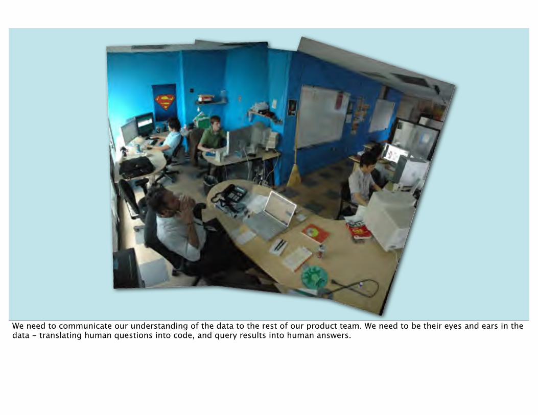
We need to communicate our understanding of the data to the rest of our product team. We need to be their eyes and ears in the data - translating human questions into code, and query results into human answers.
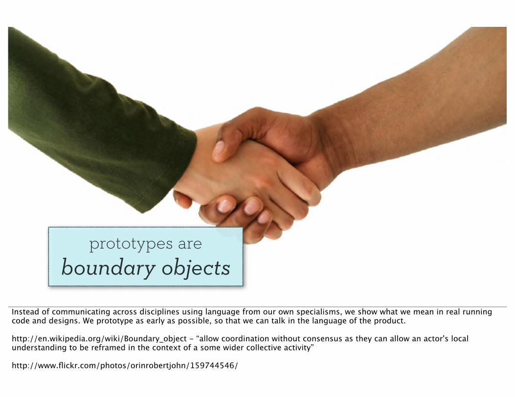
prototypes areboundary objects
Instead of communicating across disciplines using language from our own specialisms, we show what we mean in real running code and designs. We prototype as early as possible, so that we can talk in the language of the product.
http://en.wikipedia.org/wiki/Boundary_object - “allow coordination without consensus as they can allow an actor's local understanding to be reframed in the context of a some wider collective activity”
http://www.flickr.com/photos/orinrobertjohn/159744546/

Prototyping has many potential benefits. We use this triangle to think about how to structure our work and make it clear what insights we are looking for in a particular project.

Nov
elty
Prototyping has many potential benefits. We use this triangle to think about how to structure our work and make it clear what insights we are looking for in a particular project.

Fidelit
yN
ovel
ty
Prototyping has many potential benefits. We use this triangle to think about how to structure our work and make it clear what insights we are looking for in a particular project.

Fidelit
yN
ovel
tyDesirability
Prototyping has many potential benefits. We use this triangle to think about how to structure our work and make it clear what insights we are looking for in a particular project.

Fidelit
yN
ovel
tyDesirability
Prototyping has many potential benefits. We use this triangle to think about how to structure our work and make it clear what insights we are looking for in a particular project.

no morelorem ipsum
By incorporating analysis and data-science into product design during the prototyping phase, we avoid “lorem ipsum”, the fake text and made-up data that is often used as a placeholder in design sketches. This helps us understand real-world product use and find problems earlier.
Photo by R.B. - http://flic.kr/p/8APoN4
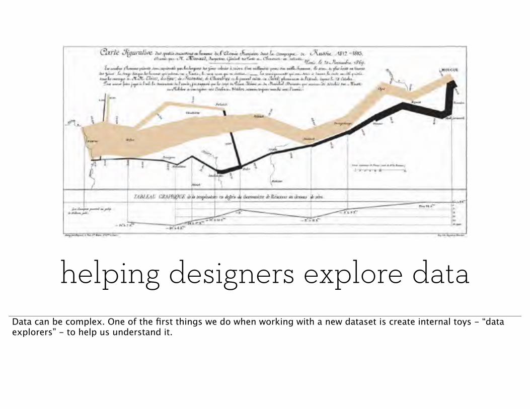
helping designers explore dataData can be complex. One of the first things we do when working with a new dataset is create internal toys - “data explorers” - to help us understand it.
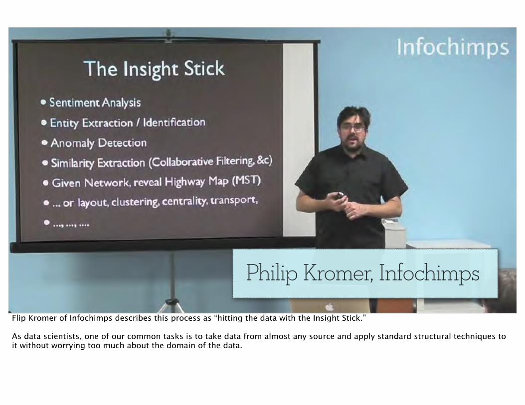
Philip Kromer, Infochimps
Flip Kromer of Infochimps describes this process as “hitting the data with the Insight Stick.”
As data scientists, one of our common tasks is to take data from almost any source and apply standard structural techniques to it without worrying too much about the domain of the data.

Philip Kromer, Infochimps
“With enough data you can discover patterns
and facts using simple counting that you can't
discover in small data using sophisticated
statistical and ML approaches.” –Dmitriy Ryaboy paraphrasing Peter Norvig on Quora
http://b.qr.ae/ijdb2G
Flip Kromer of Infochimps describes this process as “hitting the data with the Insight Stick.”
As data scientists, one of our common tasks is to take data from almost any source and apply standard structural techniques to it without worrying too much about the domain of the data.
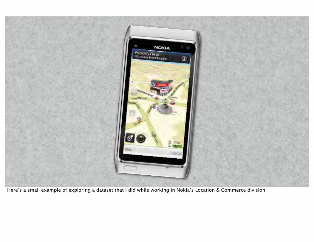
Here’s a small example of exploring a dataset that I did while working in Nokia’s Location & Commerce division.
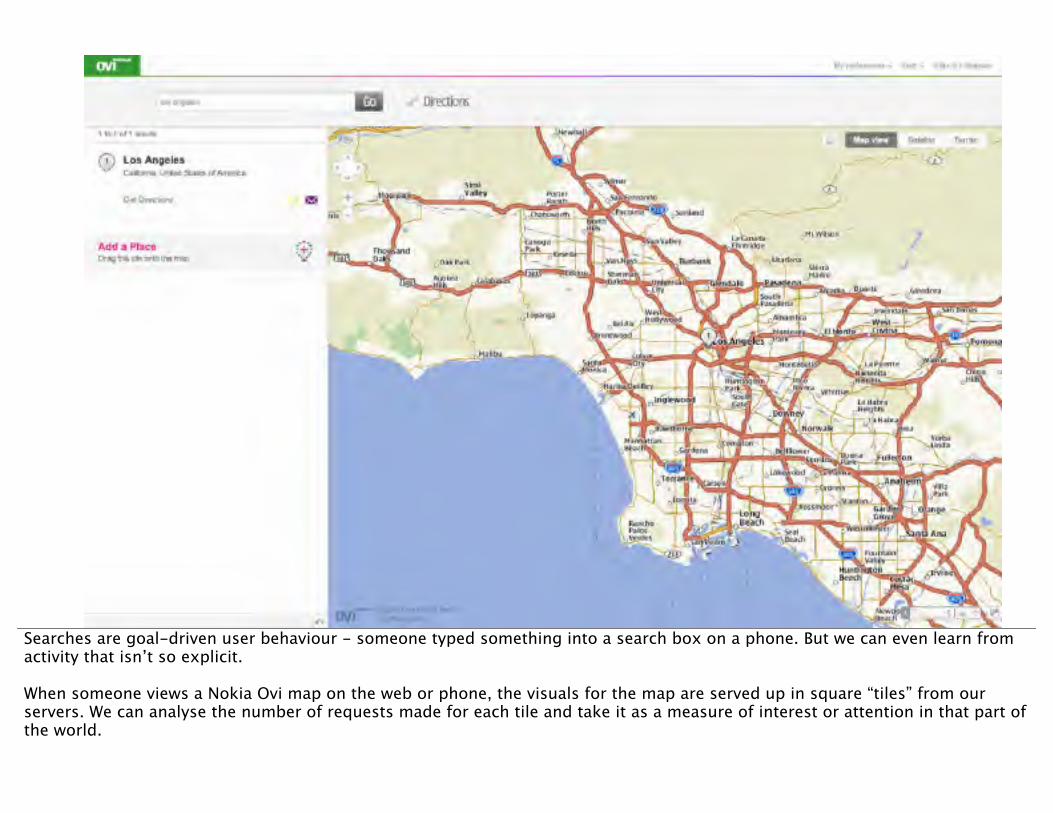
Searches are goal-driven user behaviour - someone typed something into a search box on a phone. But we can even learn from activity that isn’t so explicit.
When someone views a Nokia Ovi map on the web or phone, the visuals for the map are served up in square “tiles” from our servers. We can analyse the number of requests made for each tile and take it as a measure of interest or attention in that part of the world.
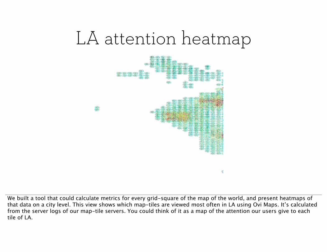
LA attention heatmap
We built a tool that could calculate metrics for every grid-square of the map of the world, and present heatmaps of that data on a city level. This view shows which map-tiles are viewed most often in LA using Ovi Maps. It’s calculated from the server logs of our map-tile servers. You could think of it as a map of the attention our users give to each tile of LA.
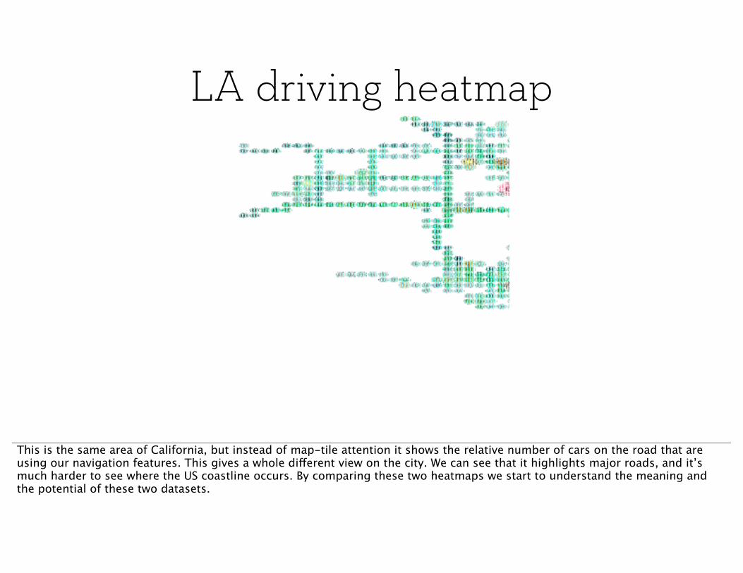
LA driving heatmap
This is the same area of California, but instead of map-tile attention it shows the relative number of cars on the road that are using our navigation features. This gives a whole different view on the city. We can see that it highlights major roads, and it’s much harder to see where the US coastline occurs. By comparing these two heatmaps we start to understand the meaning and the potential of these two datasets.
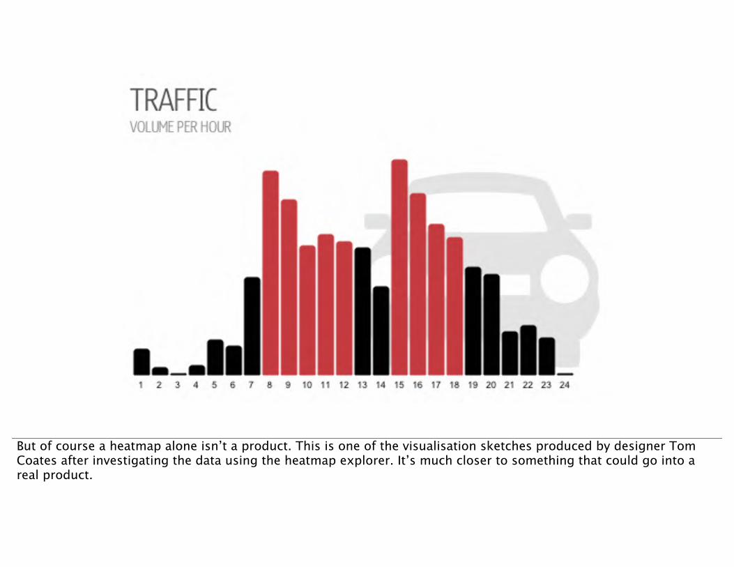
But of course a heatmap alone isn’t a product. This is one of the visualisation sketches produced by designer Tom Coates after investigating the data using the heatmap explorer. It’s much closer to something that could go into a real product.

Tools
These are the tools I’ll be using to demo some of my working processes.


Apache Pig makes Hadoop much easier to use by creating map-reduce plans from SQL-like scripts.

Elastic MapReduce and S3

With ruby scripts acting as glue for the inevitable hacking, massaging and munging of the data.

Question: who’s already working with these tools?

https://github.com/mattb/where2012-workshopAll code for the workshop:

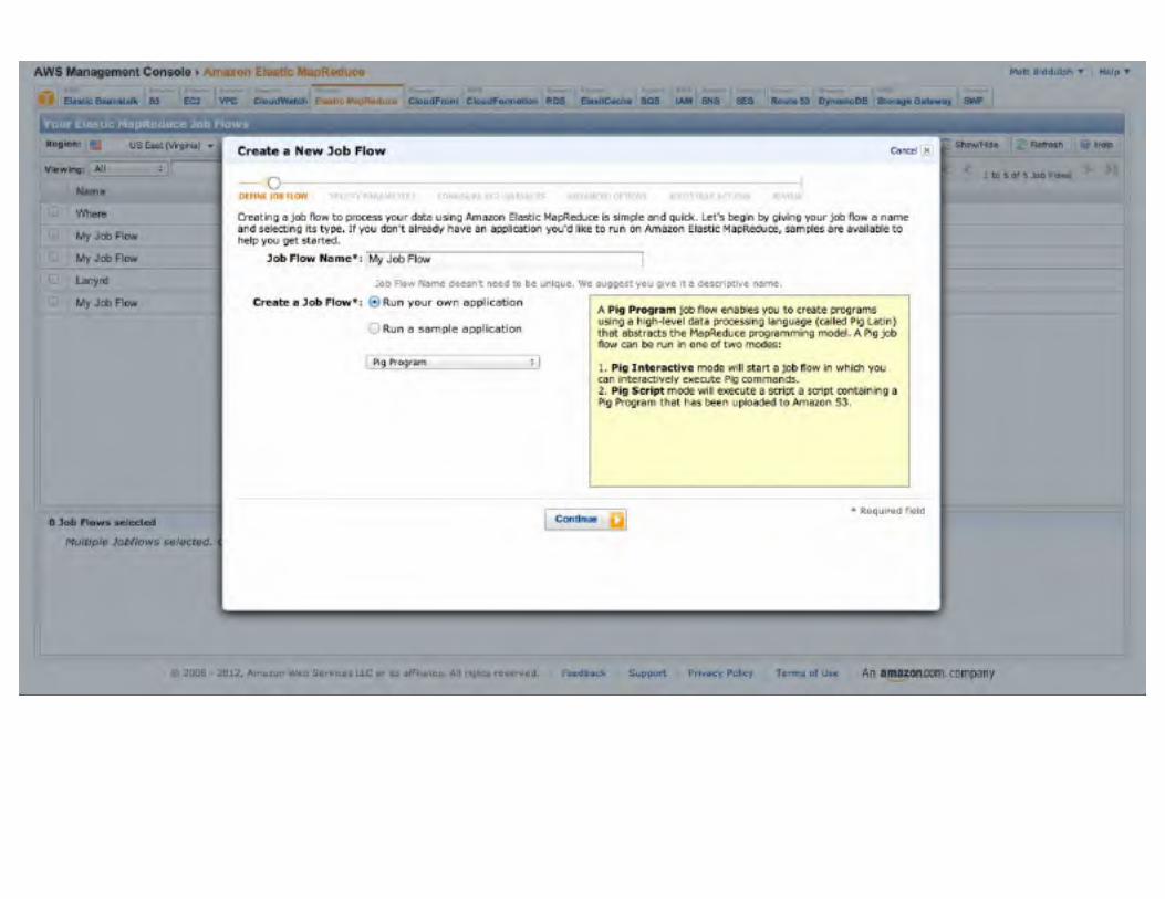
Starting up an Elastic Mapreduce clusterDemo:
Realistic cities
generating a dataset of people moving around town
The first dataset we’ll generate is one you could use to test any system or app involving people moving around the world - whether it’s an ad-targeting system or a social network.
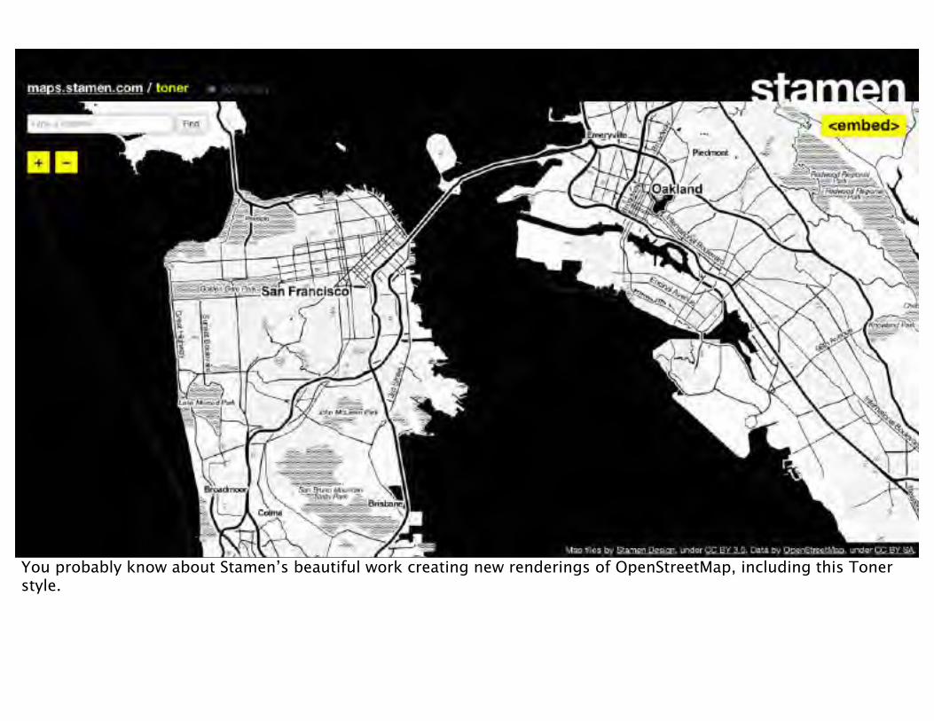
You probably know about Stamen’s beautiful work creating new renderings of OpenStreetMap, including this Toner style.
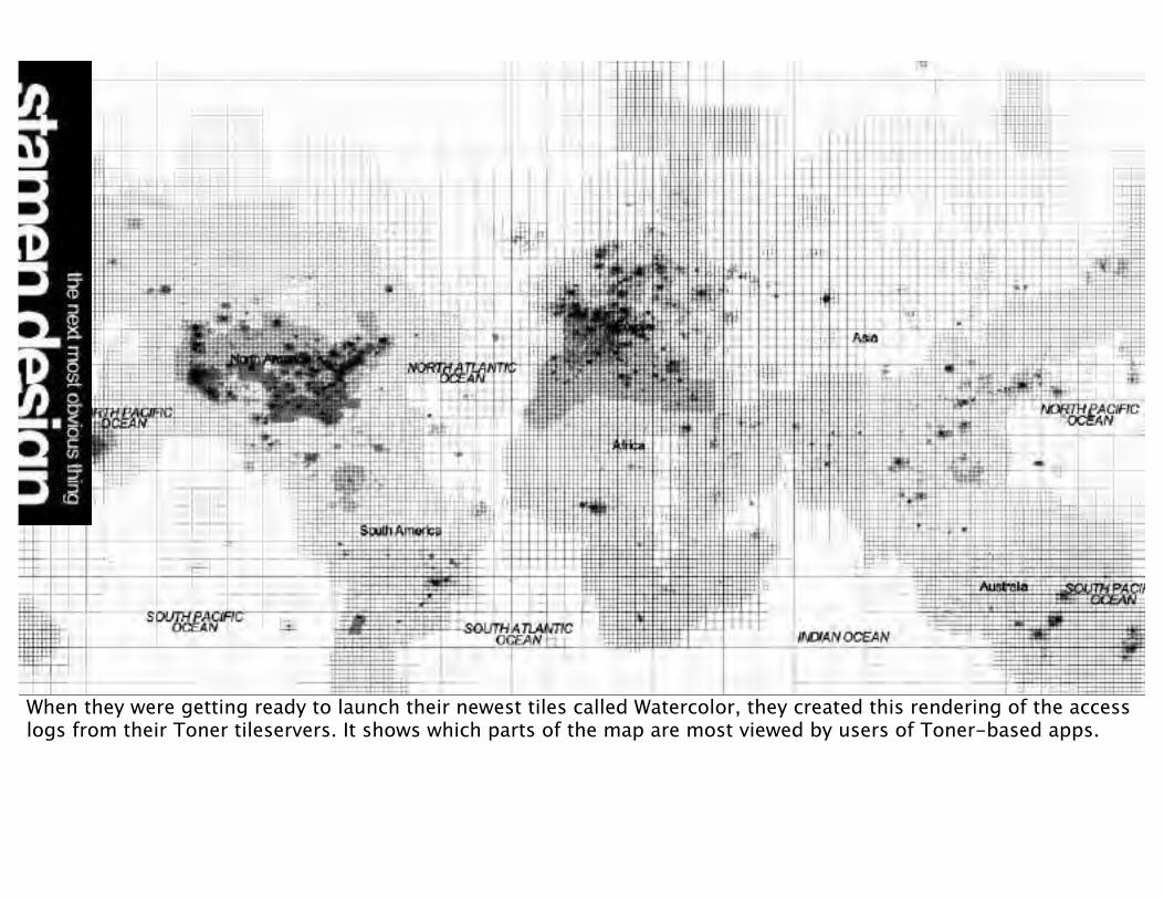
When they were getting ready to launch their newest tiles called Watercolor, they created this rendering of the access logs from their Toner tileservers. It shows which parts of the map are most viewed by users of Toner-based apps.
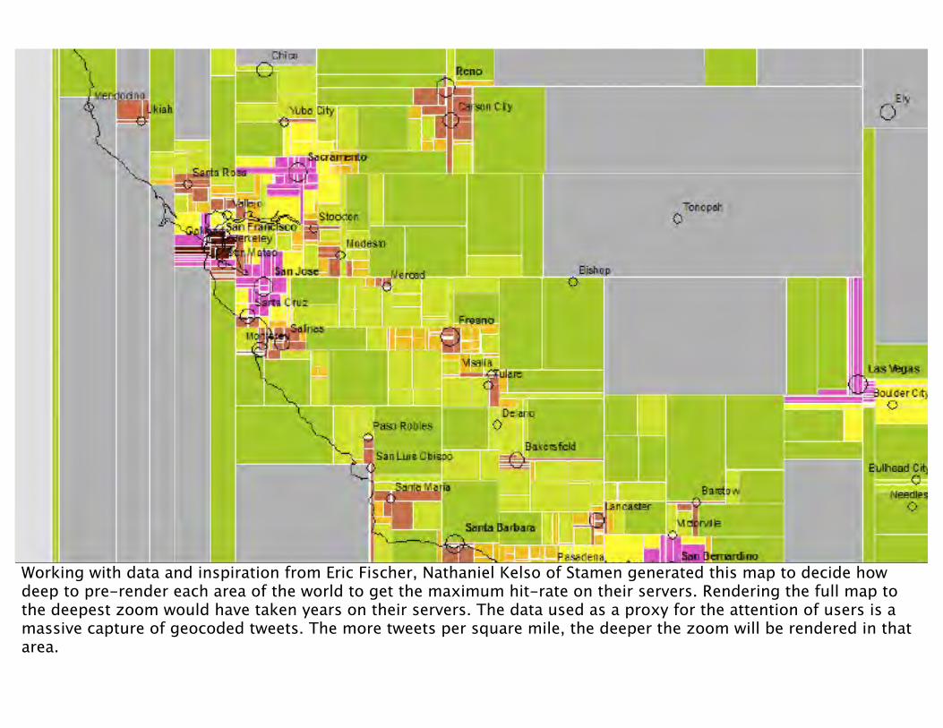
Working with data and inspiration from Eric Fischer, Nathaniel Kelso of Stamen generated this map to decide how deep to pre-render each area of the world to get the maximum hit-rate on their servers. Rendering the full map to the deepest zoom would have taken years on their servers. The data used as a proxy for the attention of users is a massive capture of geocoded tweets. The more tweets per square mile, the deeper the zoom will be rendered in that area.

We can go further than geocoded tweets and get a realistic set of POIs that people go to, with timestamps. If you search for 4sq on the Twitter streaming API you get about 25,000 tweets per hour announcing users’ Foursquare checkins.

There’s a lot of metadata available.
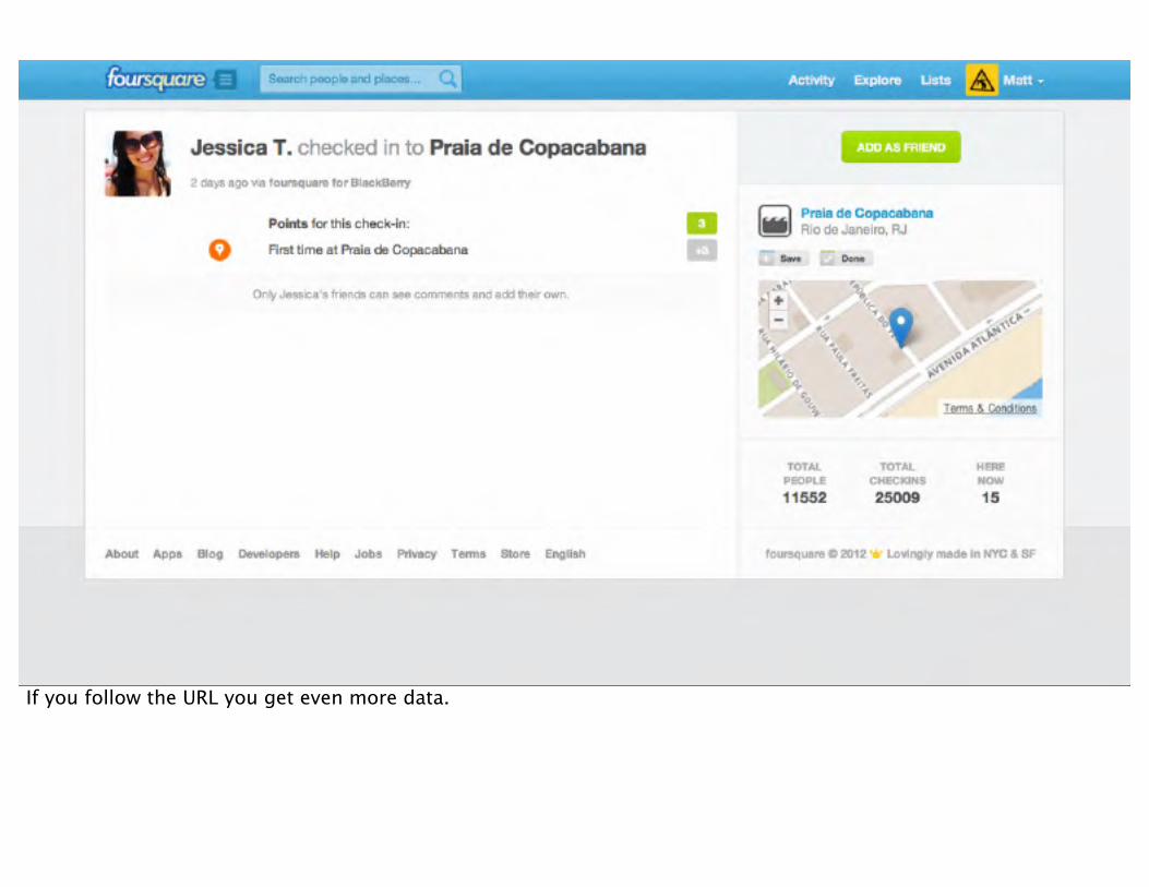
If you follow the URL you get even more data.

And if you view source, the data’s all there in JSON format.

Gathering Foursquare tweetsDemo:
So I set up a script to skim the tweets, perform the HTTP requests on 4sq.com and capture the tweet+checkin data as lines of JSON in files in S3.
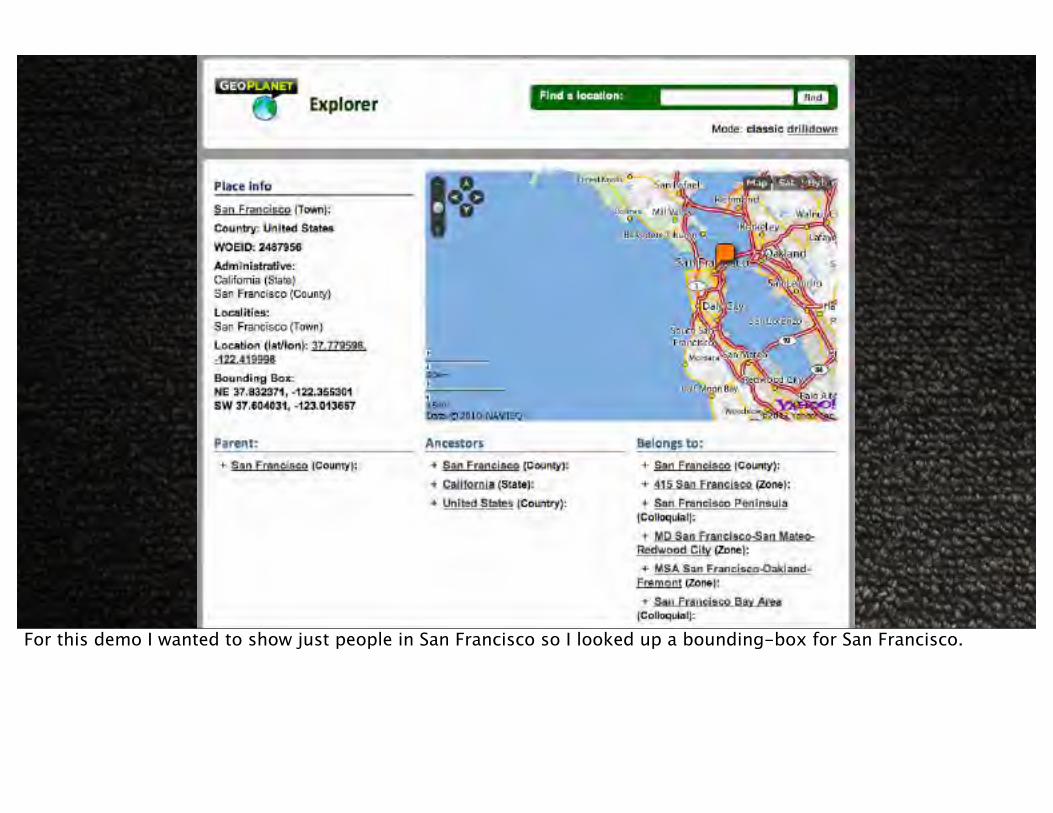
For this demo I wanted to show just people in San Francisco so I looked up a bounding-box for San Francisco.
DEFINE json2tsv `json2tsv.rb` SHIP('/home/hadoop/pig/json2tsv.rb','/home/hadoop/pig/json.tar');
A = LOAD 's3://mattb-4sq';
B = STREAM A THROUGH json2tsv AS (lat:float, lng:float, venue, nick, created_at, tweet);
SF = FILTER B BY lat > 37.604031 AND lat < 37.832371 AND lng > -123.013657 AND lng < -122.355301;
PEOPLE = GROUP SF BY nick;
PEOPLE_COUNTED = FOREACH PEOPLE GENERATE COUNT(SF) AS c, group, SF;
ACTIVE = FILTER PEOPLE_COUNTED BY c >= 5;
RESULT = FOREACH ACTIVE GENERATE group,FLATTEN(SF);
STORE RESULT INTO 's3://mattb-4sq/active-sf';
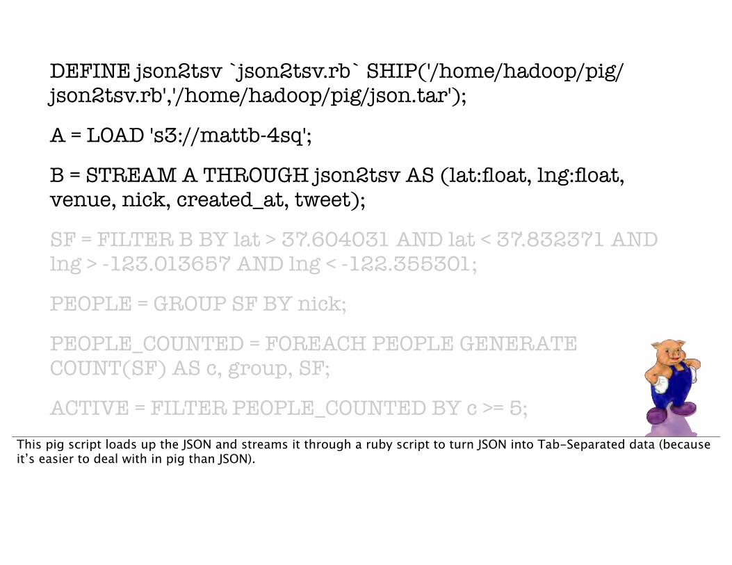
This pig script loads up the JSON and streams it through a ruby script to turn JSON into Tab-Separated data (because it’s easier to deal with in pig than JSON).
DEFINE json2tsv `json2tsv.rb` SHIP('/home/hadoop/pig/json2tsv.rb','/home/hadoop/pig/json.tar');
A = LOAD 's3://mattb-4sq';
B = STREAM A THROUGH json2tsv AS (lat:float, lng:float, venue, nick, created_at, tweet);
SF = FILTER B BY lat > 37.604031 AND lat < 37.832371 AND lng > -123.013657 AND lng < -122.355301;
PEOPLE = GROUP SF BY nick;
PEOPLE_COUNTED = FOREACH PEOPLE GENERATE COUNT(SF) AS c, group, SF;
ACTIVE = FILTER PEOPLE_COUNTED BY c >= 5;
RESULT = FOREACH ACTIVE GENERATE group,FLATTEN(SF);
STORE RESULT INTO 's3://mattb-4sq/active-sf';
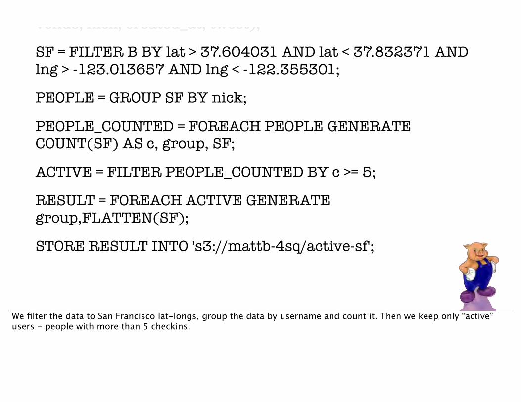
We filter the data to San Francisco lat-longs, group the data by username and count it. Then we keep only “active” users - people with more than 5 checkins.

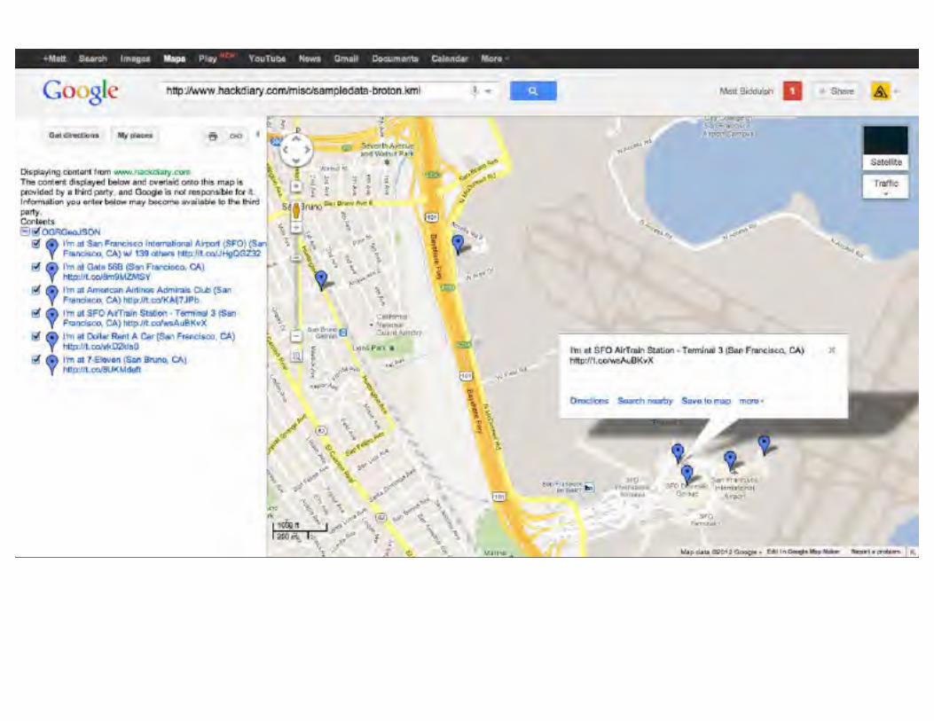
Visualising checkins with GeoJSON and KMLDemo:
You can view the path of one individual user as they arrive at SFO and get their rental car at http://maps.google.com/maps?q=http:%2F%2Fwww.hackdiary.com%2Fmisc%2Fsampledata-broton.kml&hl=en&ll=37.625585,-122.398124&spn=0.018015,0.040169&sll=37.0625,-95.677068&sspn=36.863178,82.265625&t=m&z=15&iwloc=lyrftr:kml:cFxADtCtq9UxFii5poF9Dk7kA_B4QPBI,g475427abe3071143,,
Realistic social networks
generating a dataset of social connections between people
What about the connections between people? What data could we use as a proxy for a large social graph?

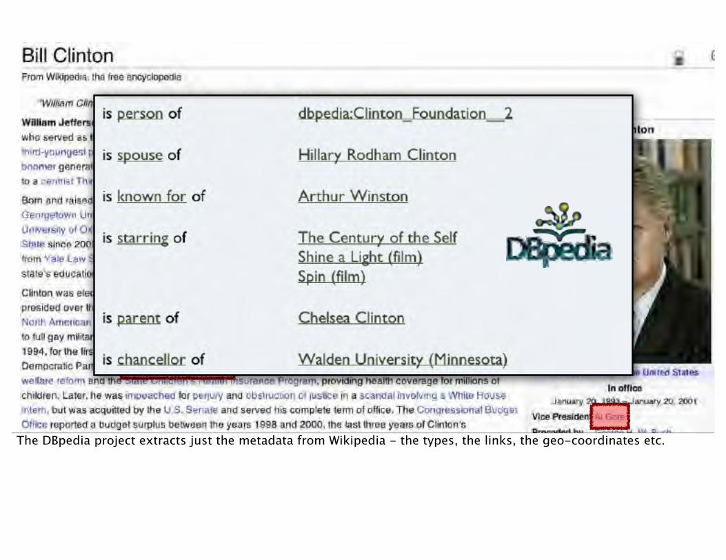
Wikipedia is full of data about people and the connections between them.
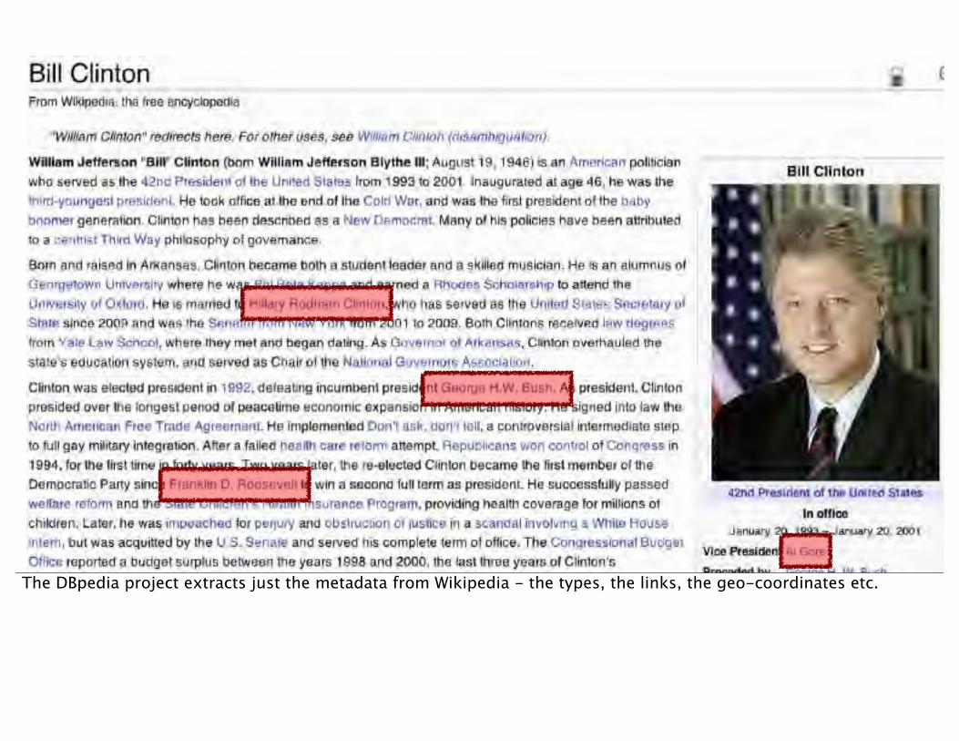
The DBpedia project extracts just the metadata from Wikipedia - the types, the links, the geo-coordinates etc.
The DBpedia project extracts just the metadata from Wikipedia - the types, the links, the geo-coordinates etc.
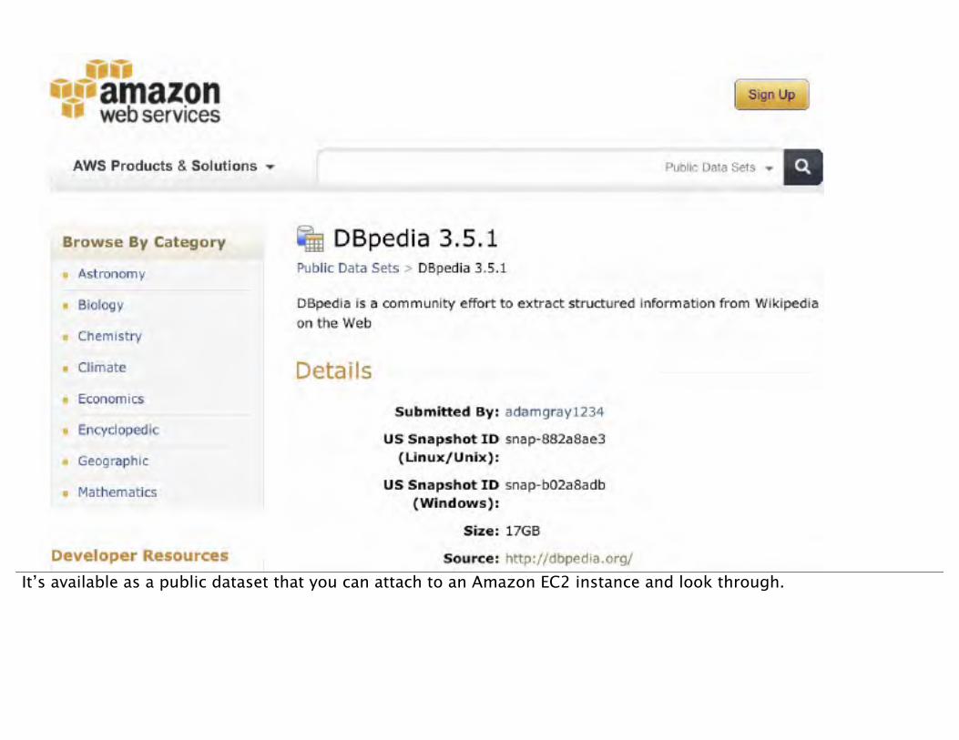
It’s available as a public dataset that you can attach to an Amazon EC2 instance and look through.
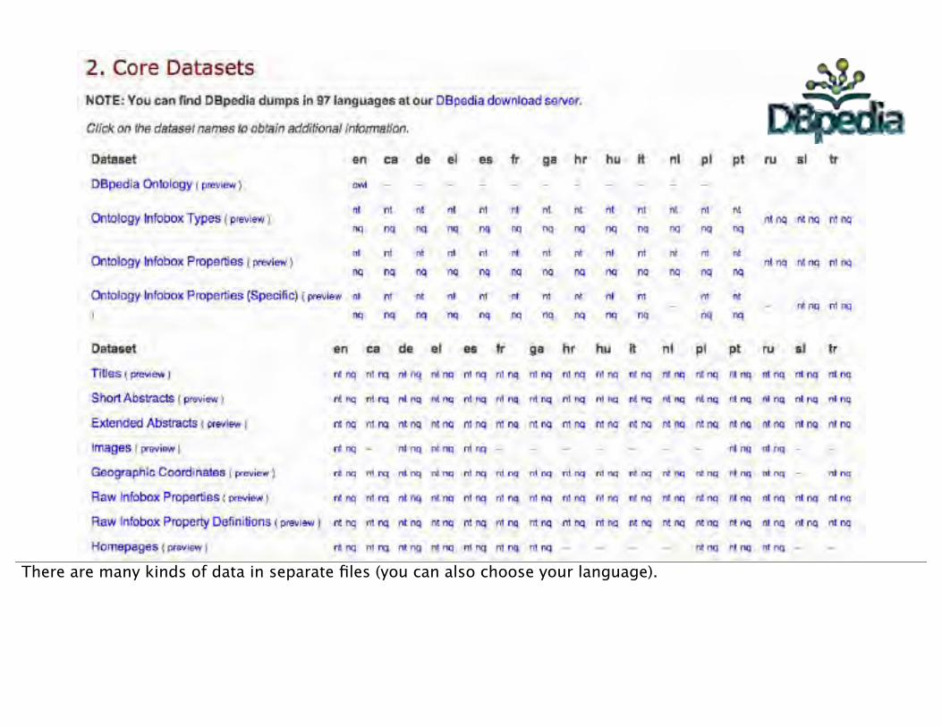
There are many kinds of data in separate files (you can also choose your language).

We’re going to start with this one. It tells us what “types” each entity is on Wikipedia, parsed out from their the Infoboxes on their pages.

<Autism> <type> <dbpedia.org/ontology/Disease> <Autism> <type> <www.w3.org/2002/07/owl#Thing> <Aristotle> <type> <dbpedia.org/ontology/Philosopher> <Aristotle> <type> <dbpedia.org/ontology/Person> <Aristotle> <type> <www.w3.org/2002/07/owl#Thing> <Aristotle> <type> <xmlns.com/foaf/0.1/Person> <Aristotle> <type> <schema.org/Person><Bill_Clinton> <type> <dbpedia.org/ontology/OfficeHolder> <Bill_Clinton> <type> <dbpedia.org/ontology/Person> <Bill_Clinton> <type> <www.w3.org/2002/07/owl#Thing> <Bill_Clinton> <type> <xmlns.com/foaf/0.1/Person> <Bill_Clinton> <type> <schema.org/Person>
Here are some examples.

<Autism> <type> <dbpedia.org/ontology/Disease> <Autism> <type> <www.w3.org/2002/07/owl#Thing> <Aristotle> <type> <dbpedia.org/ontology/Philosopher> <Aristotle> <type> <dbpedia.org/ontology/Person> <Aristotle> <type> <www.w3.org/2002/07/owl#Thing> <Aristotle> <type> <xmlns.com/foaf/0.1/Person> <Aristotle> <type> <schema.org/Person><Bill_Clinton> <type> <dbpedia.org/ontology/OfficeHolder> <Bill_Clinton> <type> <dbpedia.org/ontology/Person> <Bill_Clinton> <type> <www.w3.org/2002/07/owl#Thing> <Bill_Clinton> <type> <xmlns.com/foaf/0.1/Person> <Bill_Clinton> <type> <schema.org/Person>
And these are the ones we’re going to need; just the people.


Then we’ll take the file that shows which pages link to which other Wikipedia pages.
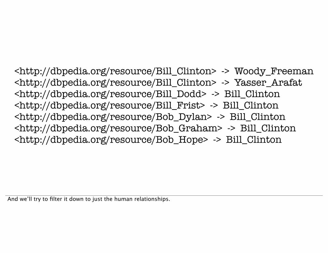
<http://dbpedia.org/resource/Bill_Clinton> -> Woody_Freeman<http://dbpedia.org/resource/Bill_Clinton> -> Yasser_Arafat<http://dbpedia.org/resource/Bill_Dodd> -> Bill_Clinton<http://dbpedia.org/resource/Bill_Frist> -> Bill_Clinton<http://dbpedia.org/resource/Bob_Dylan> -> Bill_Clinton<http://dbpedia.org/resource/Bob_Graham> -> Bill_Clinton<http://dbpedia.org/resource/Bob_Hope> -> Bill_Clinton
And we’ll try to filter it down to just the human relationships.
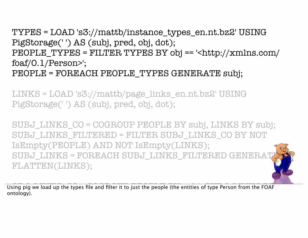
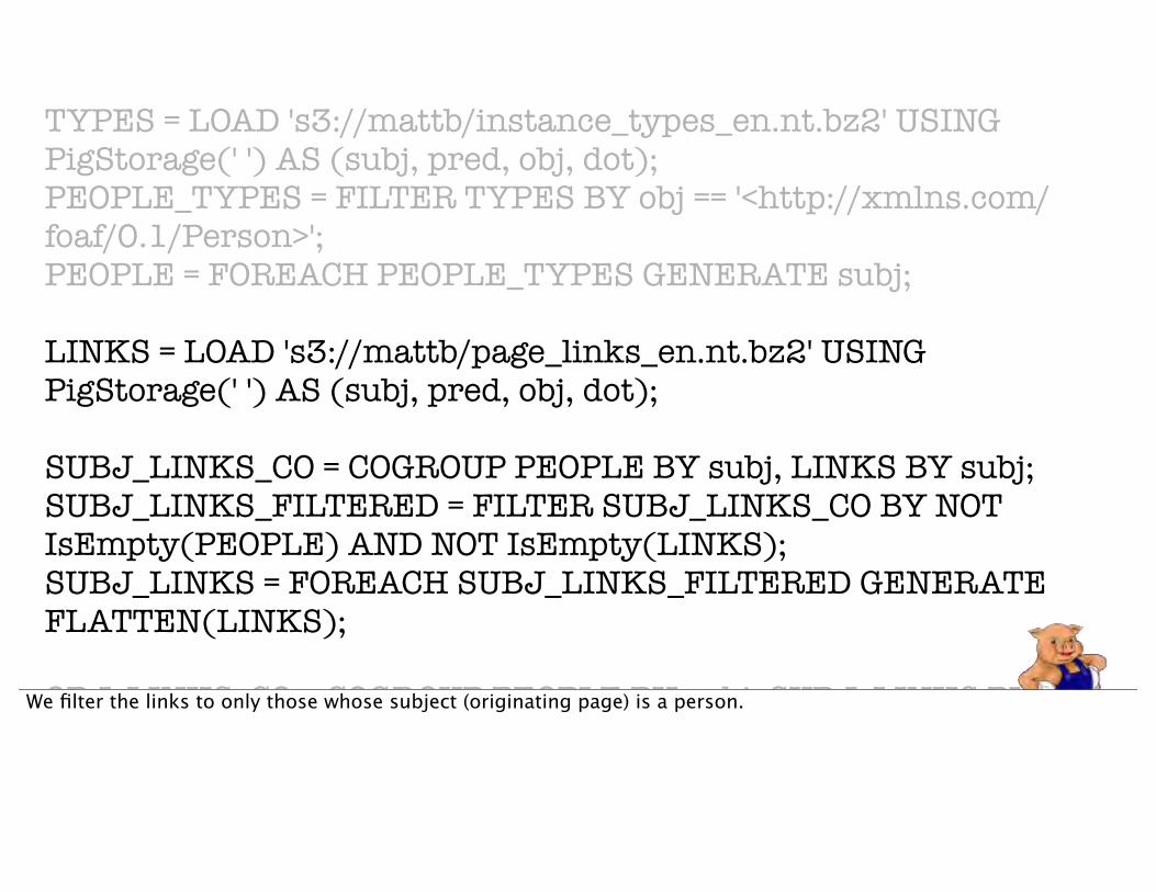
TYPES = LOAD 's3://mattb/instance_types_en.nt.bz2' USING PigStorage(' ') AS (subj, pred, obj, dot);PEOPLE_TYPES = FILTER TYPES BY obj == '<http://xmlns.com/foaf/0.1/Person>';PEOPLE = FOREACH PEOPLE_TYPES GENERATE subj;
LINKS = LOAD 's3://mattb/page_links_en.nt.bz2' USING PigStorage(' ') AS (subj, pred, obj, dot);
SUBJ_LINKS_CO = COGROUP PEOPLE BY subj, LINKS BY subj;SUBJ_LINKS_FILTERED = FILTER SUBJ_LINKS_CO BY NOT IsEmpty(PEOPLE) AND NOT IsEmpty(LINKS);SUBJ_LINKS = FOREACH SUBJ_LINKS_FILTERED GENERATE FLATTEN(LINKS);
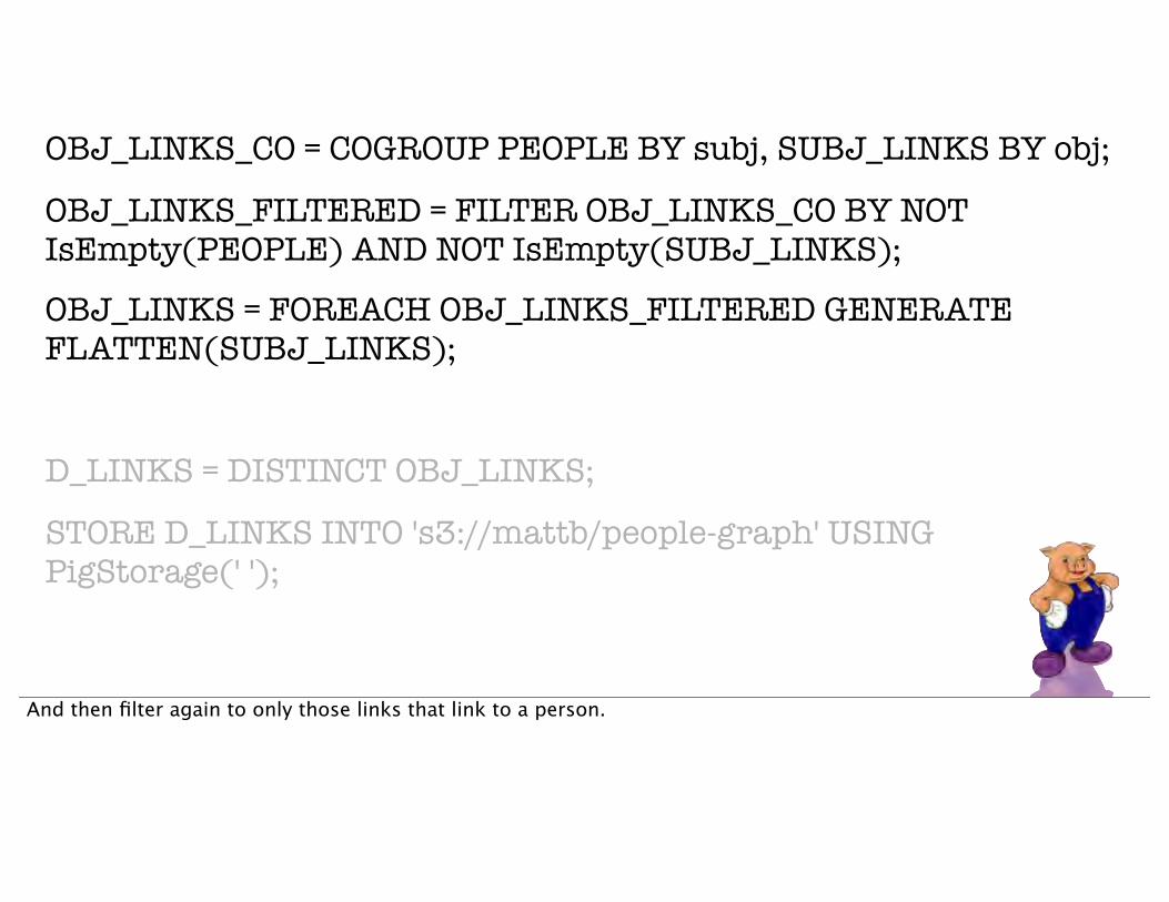
OBJ_LINKS_CO = COGROUP PEOPLE BY subj, SUBJ_LINKS BY obj;OBJ_LINKS_FILTERED = FILTER OBJ_LINKS_CO BY NOT IsEmpty(PEOPLE) AND NOT IsEmpty(SUBJ_LINKS);OBJ_LINKS = FOREACH OBJ_LINKS_FILTERED GENERATE FLATTEN(SUBJ_LINKS);
D_LINKS = DISTINCT OBJ_LINKS;
STORE D_LINKS INTO 's3://mattb/people-graph' USING PigStorage(' ');
Using pig we load up the types file and filter it to just the people (the entities of type Person from the FOAF ontology).
TYPES = LOAD 's3://mattb/instance_types_en.nt.bz2' USING PigStorage(' ') AS (subj, pred, obj, dot);PEOPLE_TYPES = FILTER TYPES BY obj == '<http://xmlns.com/foaf/0.1/Person>';PEOPLE = FOREACH PEOPLE_TYPES GENERATE subj;
LINKS = LOAD 's3://mattb/page_links_en.nt.bz2' USING PigStorage(' ') AS (subj, pred, obj, dot);
SUBJ_LINKS_CO = COGROUP PEOPLE BY subj, LINKS BY subj;SUBJ_LINKS_FILTERED = FILTER SUBJ_LINKS_CO BY NOT IsEmpty(PEOPLE) AND NOT IsEmpty(LINKS);SUBJ_LINKS = FOREACH SUBJ_LINKS_FILTERED GENERATE FLATTEN(LINKS);
OBJ_LINKS_CO = COGROUP PEOPLE BY subj, SUBJ_LINKS BY obj;OBJ_LINKS_FILTERED = FILTER OBJ_LINKS_CO BY NOT IsEmpty(PEOPLE) AND NOT IsEmpty(SUBJ_LINKS);OBJ_LINKS = FOREACH OBJ_LINKS_FILTERED GENERATE FLATTEN(SUBJ_LINKS);
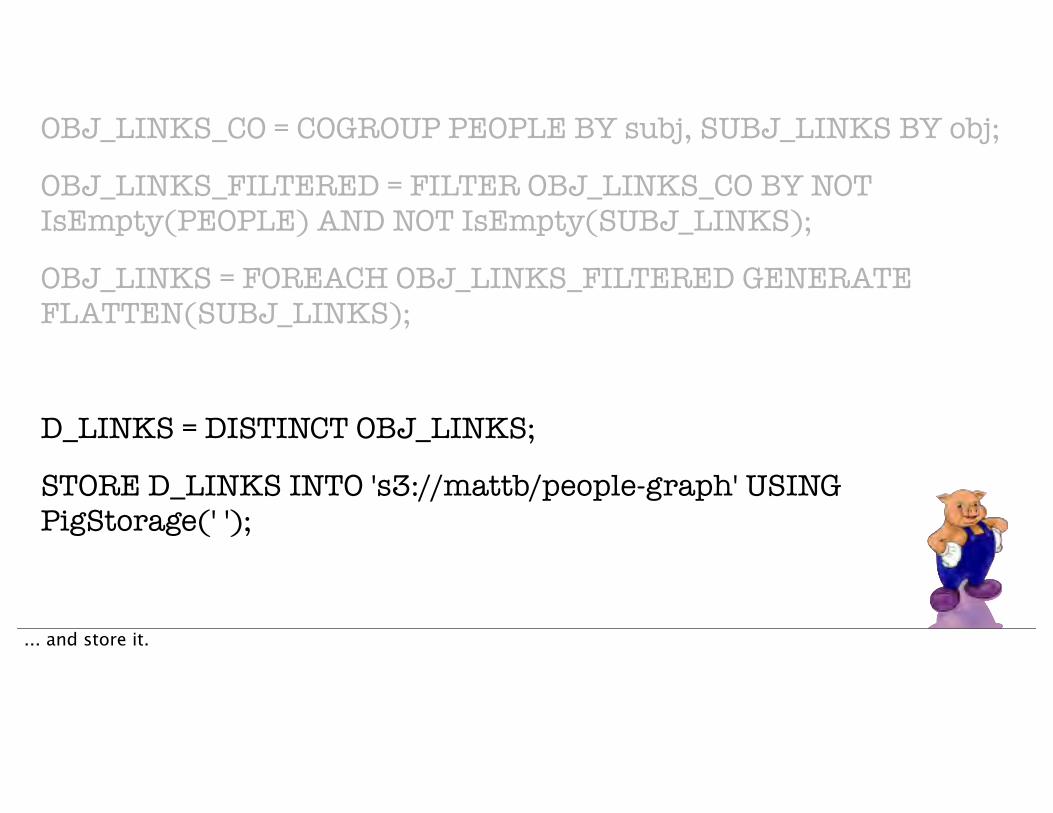
D_LINKS = DISTINCT OBJ_LINKS;
STORE D_LINKS INTO 's3://mattb/people-graph' USING PigStorage(' ');
We filter the links to only those whose subject (originating page) is a person.
LINKS = LOAD 's3://mattb/page_links_en.nt.bz2' USING PigStorage(' ') AS (subj, pred, obj, dot);
SUBJ_LINKS_CO = COGROUP PEOPLE BY subj, LINKS BY subj;
SUBJ_LINKS_FILTERED = FILTER SUBJ_LINKS_CO BY NOT IsEmpty(PEOPLE) AND NOT IsEmpty(LINKS);
SUBJ_LINKS = FOREACH SUBJ_LINKS_FILTERED GENERATE FLATTEN(LINKS);
OBJ_LINKS_CO = COGROUP PEOPLE BY subj, SUBJ_LINKS BY obj;
OBJ_LINKS_FILTERED = FILTER OBJ_LINKS_CO BY NOT IsEmpty(PEOPLE) AND NOT IsEmpty(SUBJ_LINKS);
OBJ_LINKS = FOREACH OBJ_LINKS_FILTERED GENERATE FLATTEN(SUBJ_LINKS);
D_LINKS = DISTINCT OBJ_LINKS;
STORE D_LINKS INTO 's3://mattb/people-graph' USING PigStorage(' ');
And then filter again to only those links that link to a person.
LINKS = LOAD 's3://mattb/page_links_en.nt.bz2' USING PigStorage(' ') AS (subj, pred, obj, dot);
SUBJ_LINKS_CO = COGROUP PEOPLE BY subj, LINKS BY subj;
SUBJ_LINKS_FILTERED = FILTER SUBJ_LINKS_CO BY NOT IsEmpty(PEOPLE) AND NOT IsEmpty(LINKS);
SUBJ_LINKS = FOREACH SUBJ_LINKS_FILTERED GENERATE FLATTEN(LINKS);
OBJ_LINKS_CO = COGROUP PEOPLE BY subj, SUBJ_LINKS BY obj;
OBJ_LINKS_FILTERED = FILTER OBJ_LINKS_CO BY NOT IsEmpty(PEOPLE) AND NOT IsEmpty(SUBJ_LINKS);
OBJ_LINKS = FOREACH OBJ_LINKS_FILTERED GENERATE FLATTEN(SUBJ_LINKS);
D_LINKS = DISTINCT OBJ_LINKS;
STORE D_LINKS INTO 's3://mattb/people-graph' USING PigStorage(' ');
... and store it.
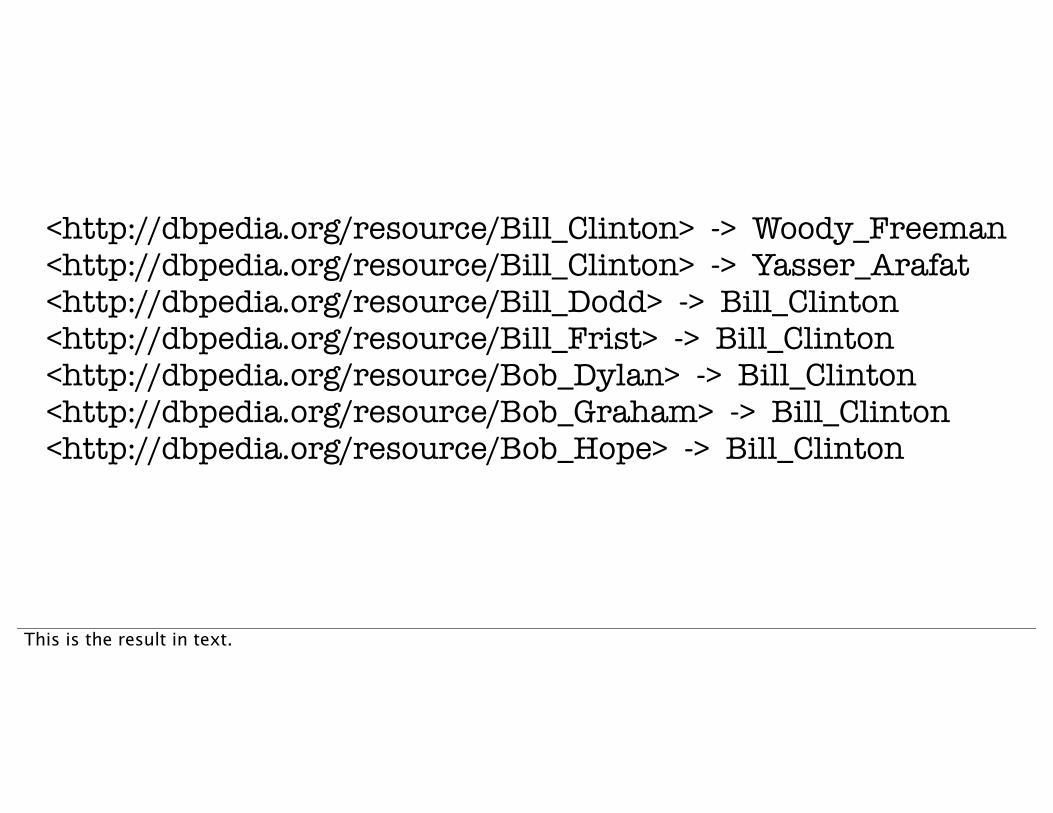
<http://dbpedia.org/resource/Bill_Clinton> -> Woody_Freeman<http://dbpedia.org/resource/Bill_Clinton> -> Yasser_Arafat<http://dbpedia.org/resource/Bill_Dodd> -> Bill_Clinton<http://dbpedia.org/resource/Bill_Frist> -> Bill_Clinton<http://dbpedia.org/resource/Bob_Dylan> -> Bill_Clinton<http://dbpedia.org/resource/Bob_Graham> -> Bill_Clinton<http://dbpedia.org/resource/Bob_Hope> -> Bill_Clinton
This is the result in text.
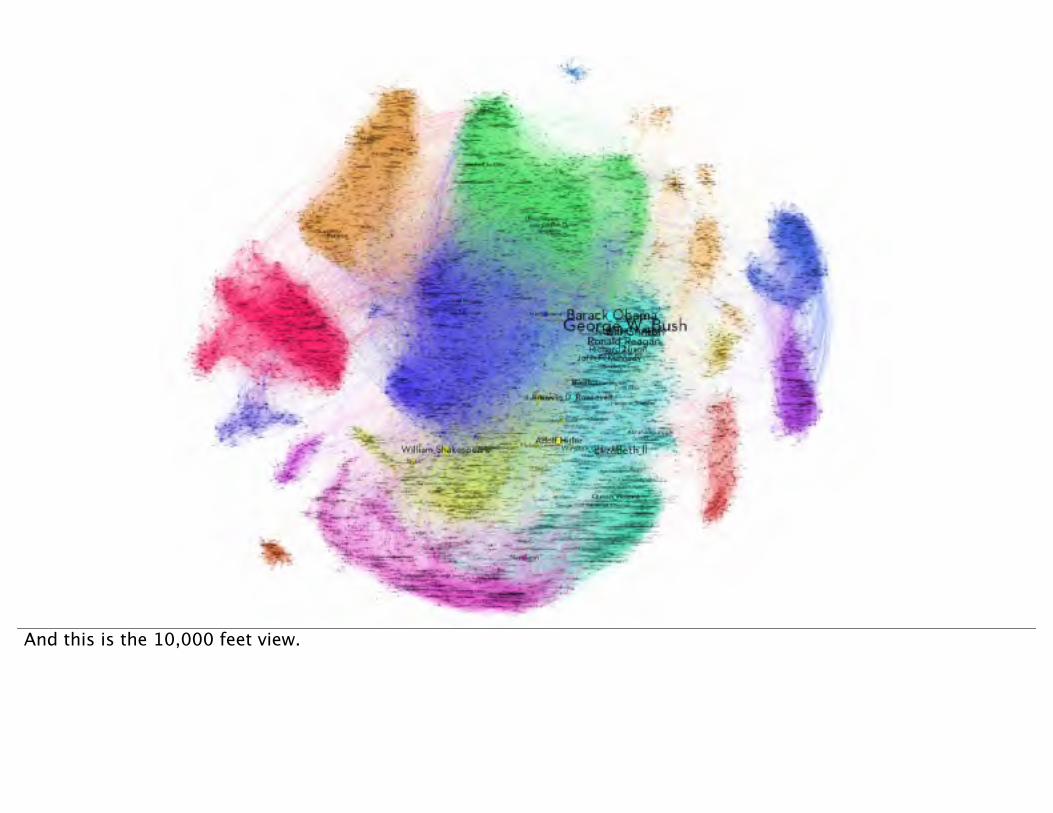
And this is the 10,000 feet view.
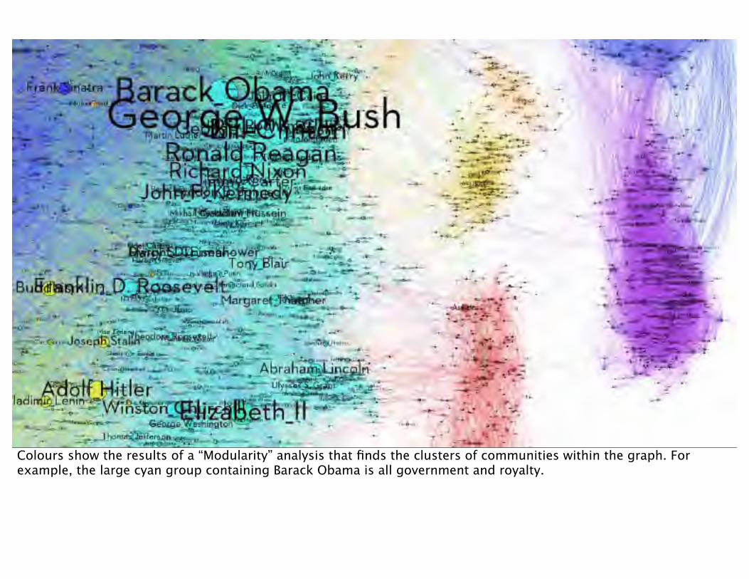
Colours show the results of a “Modularity” analysis that finds the clusters of communities within the graph. For example, the large cyan group containing Barack Obama is all government and royalty.

http://biddul.ph/wikipedia-graphExplore it yourself:

http://gephi.org
Thanks to Gephi for a great graph-visualisation tool.
This is a great book that goes into these techniques in depth. However it’s useful for any networked data, not just social networks. And it’s useful to anyone, not just startups.

This is a great book that goes into these techniques in depth. However it’s useful for any networked data, not just social networks. And it’s useful to anyone, not just startups.

This is a great book that goes into these techniques in depth. However it’s useful for any networked data, not just social networks. And it’s useful to anyone, not just startups.
Realistic ranking
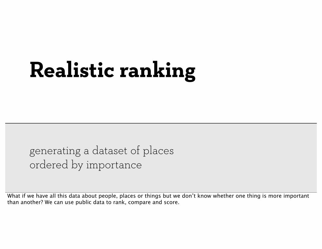
generating a dataset of places ordered by importance
What if we have all this data about people, places or things but we don’t know whether one thing is more important than another? We can use public data to rank, compare and score.
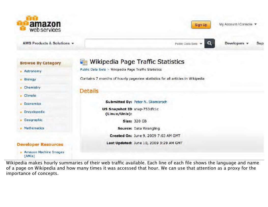
Wikipedia makes hourly summaries of their web traffic available. Each line of each file shows the language and name of a page on Wikipedia and how many times it was accessed that hour. We can use that attention as a proxy for the importance of concepts.

Back to DBpedia for some more data.

This time we’re going to extract and rank things that have geotags on their page.

<Alabama> <type> <www.opengis.net/gml/_Feature>
The geographic coordinates file lists each entity on Wikipedia that is known to have lat-long coordinates.
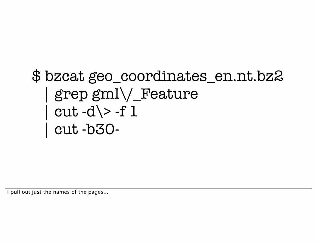
$ bzcat geo_coordinates_en.nt.bz2 | grep gml\/_Feature | cut -d\> -f 1 | cut -b30-
I pull out just the names of the pages...
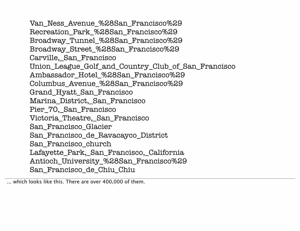
Van_Ness_Avenue_%28San_Francisco%29Recreation_Park_%28San_Francisco%29Broadway_Tunnel_%28San_Francisco%29Broadway_Street_%28San_Francisco%29Carville,_San_FranciscoUnion_League_Golf_and_Country_Club_of_San_FranciscoAmbassador_Hotel_%28San_Francisco%29Columbus_Avenue_%28San_Francisco%29Grand_Hyatt_San_FranciscoMarina_District,_San_FranciscoPier_70,_San_FranciscoVictoria_Theatre,_San_FranciscoSan_Francisco_GlacierSan_Francisco_de_Ravacayco_DistrictSan_Francisco_churchLafayette_Park,_San_Francisco,_CaliforniaAntioch_University_%28San_Francisco%29San_Francisco_de_Chiu_Chiu
... which looks like this. There are over 400,000 of them.
DATA = LOAD 's3://wikipedia-stats/*.gz' USING PigStorage(' ') AS (lang, name, count:int, other);
ENDATA = FILTER DATA BY lang=='en';
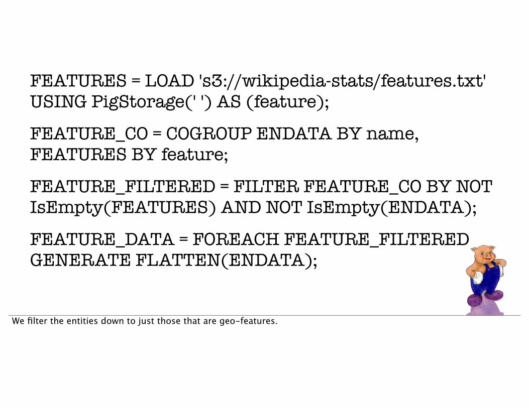
FEATURES = LOAD 's3://wikipedia-stats/features.txt' USING PigStorage(' ') AS (feature);
FEATURE_CO = COGROUP ENDATA BY name, FEATURES BY feature;
FEATURE_FILTERED = FILTER FEATURE_CO BY NOT IsEmpty(FEATURES) AND NOT IsEmpty(ENDATA);
FEATURE_DATA = FOREACH FEATURE_FILTERED GENERATE FLATTEN(ENDATA);
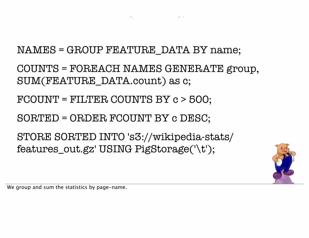
NAMES = GROUP FEATURE_DATA BY name;
COUNTS = FOREACH NAMES GENERATE group, SUM(FEATURE_DATA.count) as c;
FCOUNT = FILTER COUNTS BY c > 500;
SORTED = ORDER FCOUNT BY c DESC;
STORE SORTED INTO 's3://wikipedia-stats/features_out.gz' USING PigStorage('\t');
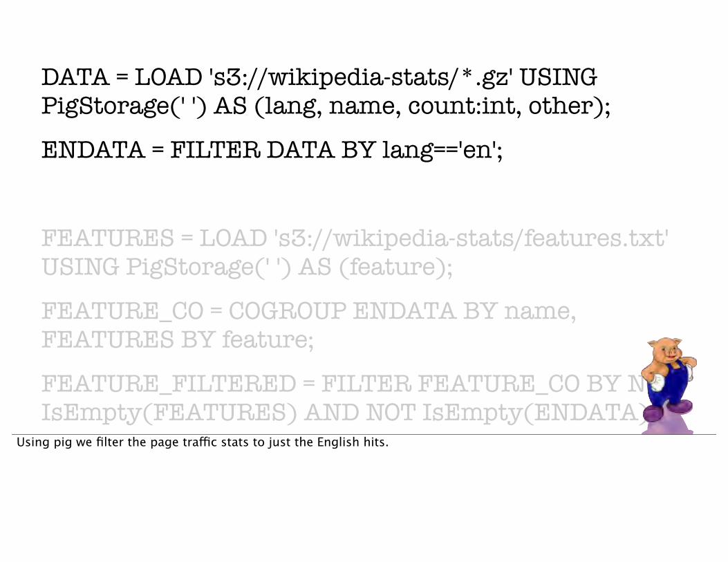
Using pig we filter the page traffic stats to just the English hits.
DATA = LOAD 's3://wikipedia-stats/*.gz' USING PigStorage(' ') AS (lang, name, count:int, other);
ENDATA = FILTER DATA BY lang=='en';
FEATURES = LOAD 's3://wikipedia-stats/features.txt' USING PigStorage(' ') AS (feature);
FEATURE_CO = COGROUP ENDATA BY name, FEATURES BY feature;
FEATURE_FILTERED = FILTER FEATURE_CO BY NOT IsEmpty(FEATURES) AND NOT IsEmpty(ENDATA);
FEATURE_DATA = FOREACH FEATURE_FILTERED GENERATE FLATTEN(ENDATA);
NAMES = GROUP FEATURE_DATA BY name;
COUNTS = FOREACH NAMES GENERATE group, SUM(FEATURE_DATA.count) as c;
FCOUNT = FILTER COUNTS BY c > 500;
SORTED = ORDER FCOUNT BY c DESC;
STORE SORTED INTO 's3://wikipedia-stats/features_out.gz' USING PigStorage('\t');
We filter the entities down to just those that are geo-features.
DATA = LOAD 's3://wikipedia-stats/*.gz' USING PigStorage(' ') AS (lang, name, count:int, other);
ENDATA = FILTER DATA BY lang=='en';
FEATURES = LOAD 's3://wikipedia-stats/features.txt' USING PigStorage(' ') AS (feature);
FEATURE_CO = COGROUP ENDATA BY name, FEATURES BY feature;
FEATURE_FILTERED = FILTER FEATURE_CO BY NOT IsEmpty(FEATURES) AND NOT IsEmpty(ENDATA);
FEATURE_DATA = FOREACH FEATURE_FILTERED GENERATE FLATTEN(ENDATA);
NAMES = GROUP FEATURE_DATA BY name;
COUNTS = FOREACH NAMES GENERATE group, SUM(FEATURE_DATA.count) as c;
FCOUNT = FILTER COUNTS BY c > 500;
SORTED = ORDER FCOUNT BY c DESC;
STORE SORTED INTO 's3://wikipedia-stats/features_out.gz' USING PigStorage('\t');
We group and sum the statistics by page-name.
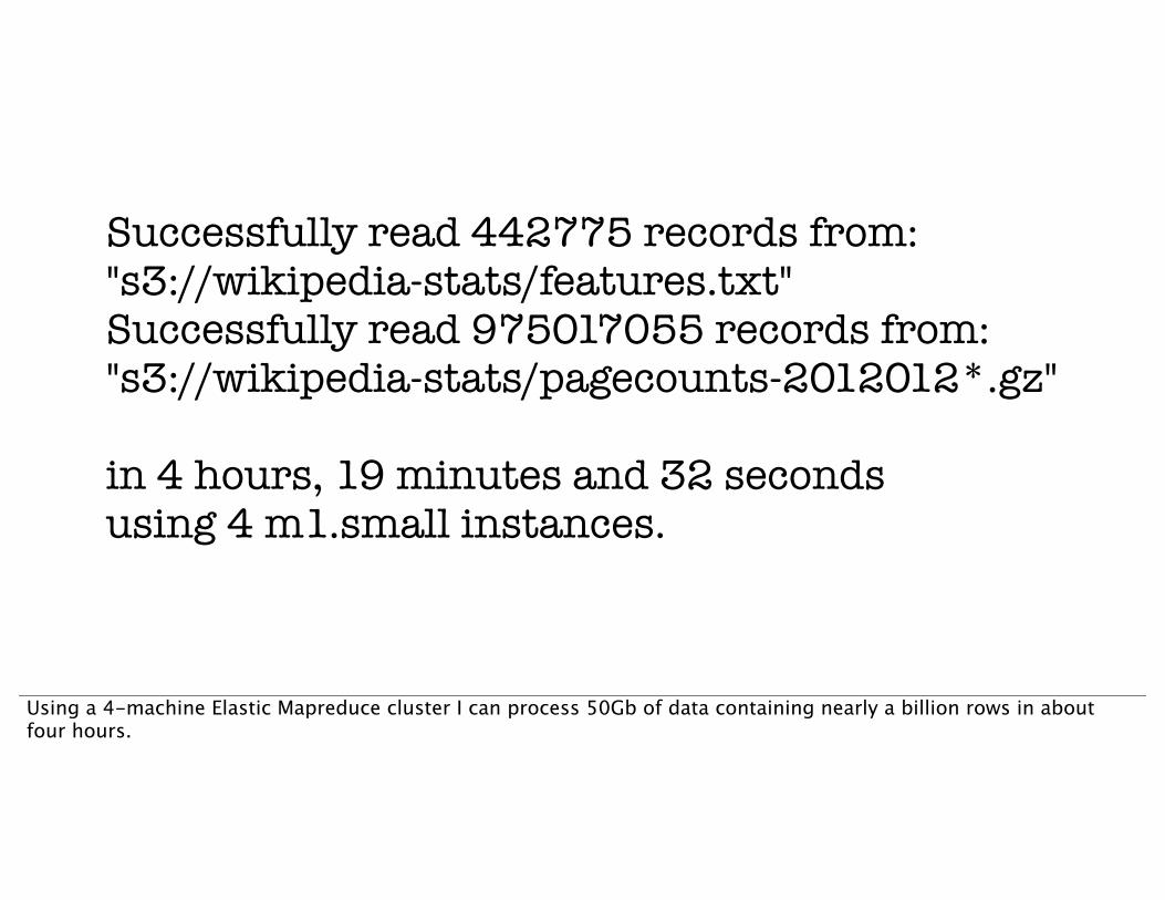
Successfully read 442775 records from: "s3://wikipedia-stats/features.txt"Successfully read 975017055 records from: "s3://wikipedia-stats/pagecounts-2012012*.gz"
in 4 hours, 19 minutes and 32 secondsusing 4 m1.small instances.
Using a 4-machine Elastic Mapreduce cluster I can process 50Gb of data containing nearly a billion rows in about four hours.
The Castro
Chinatown
Tenderloin
Mission District
Union Square
Nob Hill
Bayview-Hunters Point
Alamo Square
Russian Hill
Ocean Beach
Pacific Heights
Sunset District0 750 1500 2250 3000
573
592
661
721
768
916
952
1283
1336
2276
2457
2479
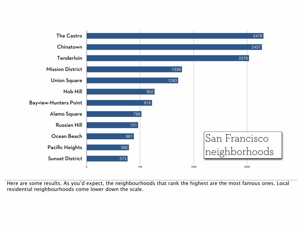
San Francisco neighborhoods
Here are some results. As you’d expect, the neighbourhoods that rank the highest are the most famous ones. Local residential neighbourhoods come lower down the scale.
Hackney
Camden
Tower Hamlets
Newham
Enfield
Croydon
Islington
Southwark
Lambeth
Greenwich
Hammersmith and Fulham
Haringey
Harrow
Brent0 1000 2000 3000 4000
1140
1183
1263
1268
1316
1354
1603
1624
1796
1830
1850
2378
2498
3428
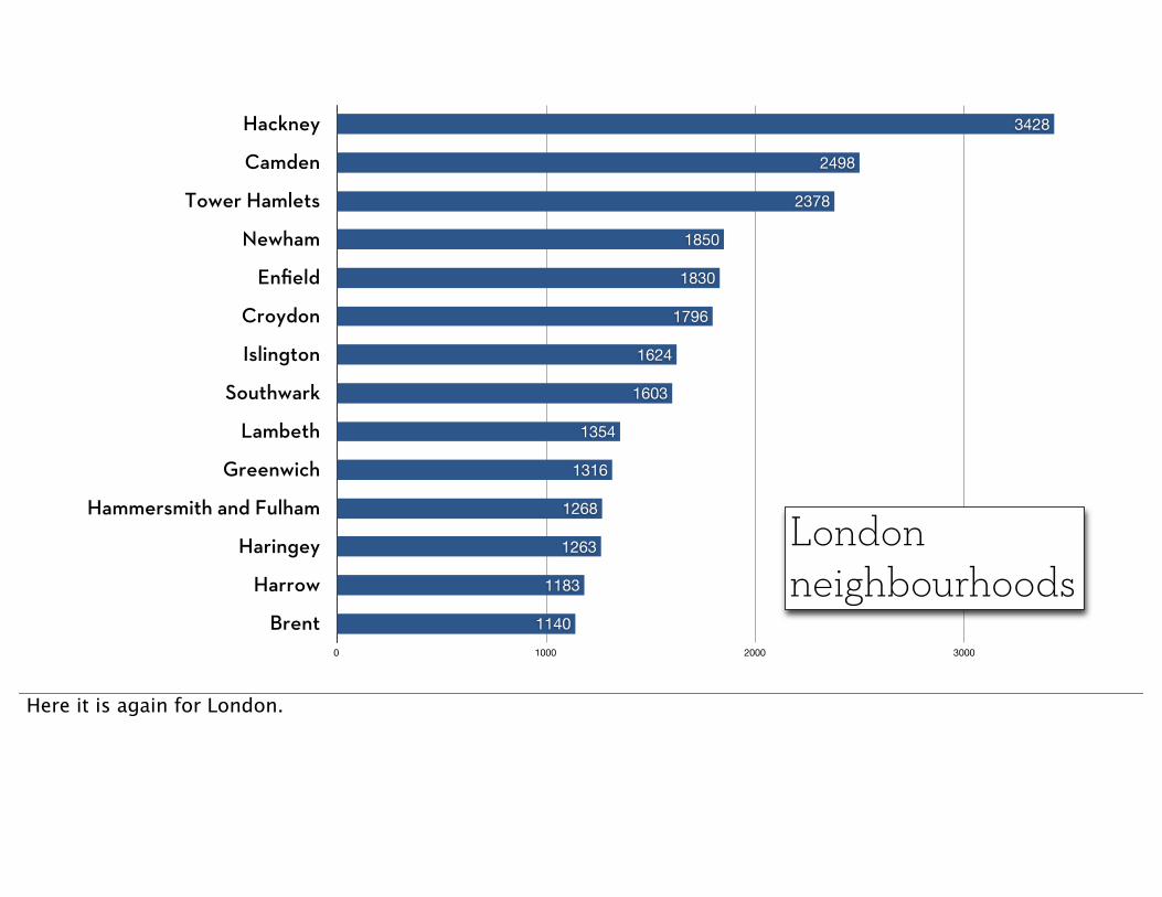
Londonneighbourhoods
Here it is again for London.

To demo this ranking in a data toy that anyone can play with, I built an auto-completer using Elasticsearch. I transformed the pig output into JSON and made an index.

A weighted autocompleter with ElasticsearchDemo:
I exposed this index through a small Ruby webapp written in Sinatra.
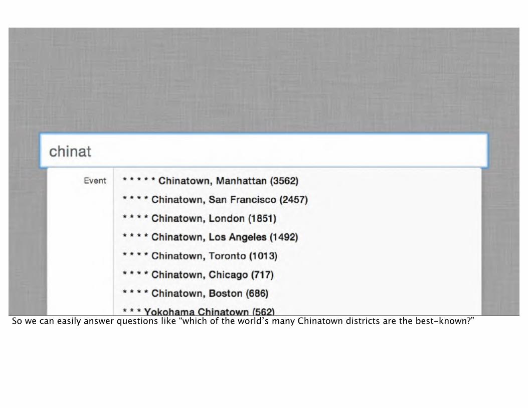
So we can easily answer questions like “which of the world’s many Chinatown districts are the best-known?”

https://github.com/mattb/where2012-workshopAll code for the workshop: