Proving Probabilistic Correctness Statements: the Case

of Rabin’s Algorithm for Mutual Exclusion*

Isaac Saiast

Laboratory for Computer Science

Massachusetts Institute of Technology

Cambridge, MA 02139

Abstract

The correctness of most randomized distributed algo-

rithms is expressed by a statement of the form “some

predicate of the executions holds with high probabil-

ity, regardless of the order in which actions are sched-

uled”. In this paper, we present a general methodol-

ogy to prove correctness statements of such random-

ized algorithms. Specifically, we show how to prove

such statements by a series of refinements, which ter-

minate in a statement independent of the schedule.

To demonstrate the subtlety of the issues involved in

this type of analysis, we focus on Rabin’s randomized

distributed algorithm for mutual exclusion [6].

Surprisingly, it turns out that the algorithm does

not maintain one of the requirements of the problem

under a certain schedule. In particular, we give a

schedule under which a set of processes can suffer

lockout for arbitrary long periods.

1 Introduction

1.1 General Considerations

For many distributed system problems, it is possi-

ble to produce randomized algorithms that are bet-

ter than their deterministic counterparts: they may

be more efficient, have simpler structure, and even

achieve correctness properties that deterministic al-

*Research supported by research contracts ONR-NOOO14-91-J-1046, NSF-CCR-S915206 and DARPA-NOO014-89-J-1988.

te-~~1: saiasetheory. lcs .rnit. edu

Permission to copy without fee all or part of this material ia

granted provided that the copies are not mada or distributed for

direct commercial advantage, the ACM copyright notice and tha

title of tha publication and its date appear, and notica is given

that copying is by permission of the Association for ComputingMachinery. To copY otherwise, or to republish, requires a fee

and/or specific permission.

poDG ‘92-81921B.C.

~ 1992 ACM 0-89791 -496- 1/92/000810263 . . ..S1.50

gorithms cannot. One cost of using randomization is

the increased difficulty of proving correctness of the

resulting algorithms. A randomized algorithm typi-

cally involves two different types of nondeterminism

- that arising from the random choices and that aris-

ing from an adversary. The interaction between these

two kinds of nondeterminism complicates the analysis

of the algorithm.

In the distributed system model considered here,

each of a set of concurrent processes executes ita lo-

cal code and communicates with the others through

a shared variable. The code can contain random

choices, which leads to probabilistic branch points in

the tree of executions. By assumption, the algorithm

is provided at certain points of the execution with

random inputs having known distributions. We can

equivalently consider that all random choices made

in a single execution are given by a parameter w at

the onset of the execution. The parameter w thus

captures the first type of nondeterminism.

For the second type, we here define the adversary

d to be the entity controlling the order in which pro-

cesses take steps. (In other work (e.g., [4]), the adver-

sary can control other decisions, such as the contents

of some messages. ) An adversary A basea its choices

on the knowledge it holds about the prior execution

of the system. This knowledge varies according to

the specifications for each given problem. In this pa-

per, we will consider an adversary allowed to observe

only certain “external” manifestations of the execu-

tion and having no access, for example, to informa-

tion about local process states. We will say that an

adversary is admissible to emphasize its specificity,

These two sources of nondeterminism, w and d,

uniquely define an execution f = &(w, A) of the al-

gorithm.

Among the correctness properties one often wishes

to prove for randomized algorithms are properties

that atate that a certain property W of executions

has a “high” probability of holding against all ad-

missible adversaries. Note that the probability men-

263

tioned in this statement is taken with respect to a

probability distribution on executions. One of the

major sources of complication is that there are two

probability spaces that need to be considered: the

space of random inputs w and the space of random

executions. Let dP denote the probability measure

given for the space of random inputs u.

Since the evolution of the system is determined

both by the (random) choices expressed by w and also

by the adversary A, we do not have a single probabil-

ityy distribution on the space of all executions. Rather,

for each adversary A there is a corresponding distri-

bution dP~ on the executions “compatible with” A.

High probability correctness properties of a random-

ized algorithm C are then generally stated in terms

of the distributions dPA, in the following form. Let

W and I be sets of executions of C and let 1 be a

real number in [0, 1]. Then C is correct provided that

Pd [W \ 1] ~ i for every admissible adversary A. For

a condition expressed in this form, we think of W as

the set of “good” (or “winning”) executions, while 1

is a set that expresses the assumptions under which

the good behavior is supposed to hold.

In general, it is difficult to calculate (good bounds

on) probabilities of the form PA [Wll]. This is be-

cause the probability that the execution is in W, I

or W n 1 depends on a combination of the choices

in u and those made by the adversary. Although we

assume a basic probability distribution P for w, the

adversary’s choices are determined in a more compli-

cated way – in terms of certain kinds of knowledge

of the prior execution. In particular, the adversary’s

choices can depend on the outcomes of prior random

choices made by the processes.

The situation is much simpler in the special case

where the events W and I are defined directly in

terms of the choices in w. In this case, the desired

probability can be calculated just by using the ss-

sumed probability distribution dP.

Our general methodology for proving a high prob-

ability correctness property of the form PA [W 11] con-

sists of proving successive lower bounds:

> PA[wr I 1,],

where all the Wi and Ii are sets of executions, and

where the last two sets, Wr and Ir, are defined di-

rectly in terms of the choices in w. The final term,

PA [Wr I 1,], is then evaluated (or bounded from be-

low) using the distribution dP. This methodology can

be difficult to implement as it involves disentangling

the ways in which the random choices made by the

processes affect the choices made by the adversary.

This paper is devoted to emphasizing the need of

such a rigorous methodology in correctness proofs:

in the context of randomized algorithms the power

of the adversary is generally hard to analyze and im-

precise arguments can easily lead to incorrect state-

ments.

As evidence supporting our point, we give an anal-

ysis of Rabin’s randomized distributed algorithm [6]

implementing mutual exclusion for n processes using

a read-modify-write primitive on a shared variable

with O(log n) values. Rabin claimed that the al-

gorithm satisfies the following correctness property:

for every adversary, any process competing for en-

trance to the critical section succeeds with probabil-

ity C?(l/m), where m is the number of competing pro-

cesses. As we shall see, this property can be expressed

in the general form PA [W ] X ~ 1. In [5], Sharir et

al. gave another analysis of the algorithm, providing

a formal model in terms of Markov chains; however,

they did not make explicit the influence of the adver-

sary on the probability distribution on executions.

We show that this influence is crucial: the adver-

sary in [6] is much stronger than previously thought,

and in fact, the high probability correctness result

claimed in [6] does not hold.

1.2 Rabin’s Algorithm

The problem of mutual exclusion [2] involves allocat-

ing an indivisible, reusable resource among n com-

peting processes. A mutual exclusion algorithm is

said to guarantee progressl if it continues to allo-

cate the resource as long as at least one process is

requesting it. It guarantees no-lockout if every pro-

cess that requests the resource eventually receives it.

A mutual exclusion algorithm satisfies bounded wait-

ing if there is a fixed upper bound on the number of

times any competing process can be bypassed by any

other process. In conjunction with the progress prop-

erty, the bounded waiting property implies the no-

lockout property. In 1982, Burns et al.[1] considered

the mutual exclusion algorithm in a distributed set-

ting where processes communicate through a shared

read-modify-write variable. For this setting, they

proved that any deterministic mutual exclusion alg~

rithm that guarantees progress and bounded waiting

requires that the shared variable take on at least n

distinct values. Shortly thereafter, Rabin published

a randomized mutual exclusion algorithm [6] for the

same shared memory distributed setting. His algo-

rithm guarantees progress using a shared variable

that takes on only O(log n) values.

It is quite easy to verify that Rabin’s algorithm

1We give more formal definitions of these properties in Sec-tion 2.

264

guarantees mutual exclusion and progress; in addi-

tion, however, Rabin claimed that his algorithm sat-

isfies the following informally-stated strong no-lockout

property2.

“If process i participates in a trying round

of a run of a computation by the protocol

and compatible with the adversary, together

with O < m— 1 < n other processes, then the

probability that i enters the critical region at

the end of that round is at least c/m, c N

2/3.” (*)

This property says that the algorithm guarantees

an approximately equal chance of success to all pro-

cesses that compete at the given round. Rabin argued

in [6] that a good randomized mutual exclusion alge

rithm should satisfy this strong no-lockout property,

and in particular, that the probability of each process

succeeding should depend inversely on m, the num-

ber of actual competitors at the given round. This

dependence on m was claimed to be an important ad-

vantage of this algorithm over another algorithm de-

veloped by Ben-or (also described in [6]); Ben-Or’s

algorithm is claimed to satisfy a weaker no-lockout

property in which the probability of success is approx-

imately c/n, where n is the total number of processes,

i.e., the number of potential competitors.

Rabin’s algorithm uses a randomly-chosen round

number to conduct a competition for each round.

Within each round, competing processes choose lot-

tery numbers randomly, according to a truncated ge-

ometric distribution. One of the processes drawing

the largest lottery number for the round wins. Thus,

randomness is used in two ways in this algorithm:

for choosing the round numbers and choosing the lot-

tery numbers. The detailed code for this algorithm

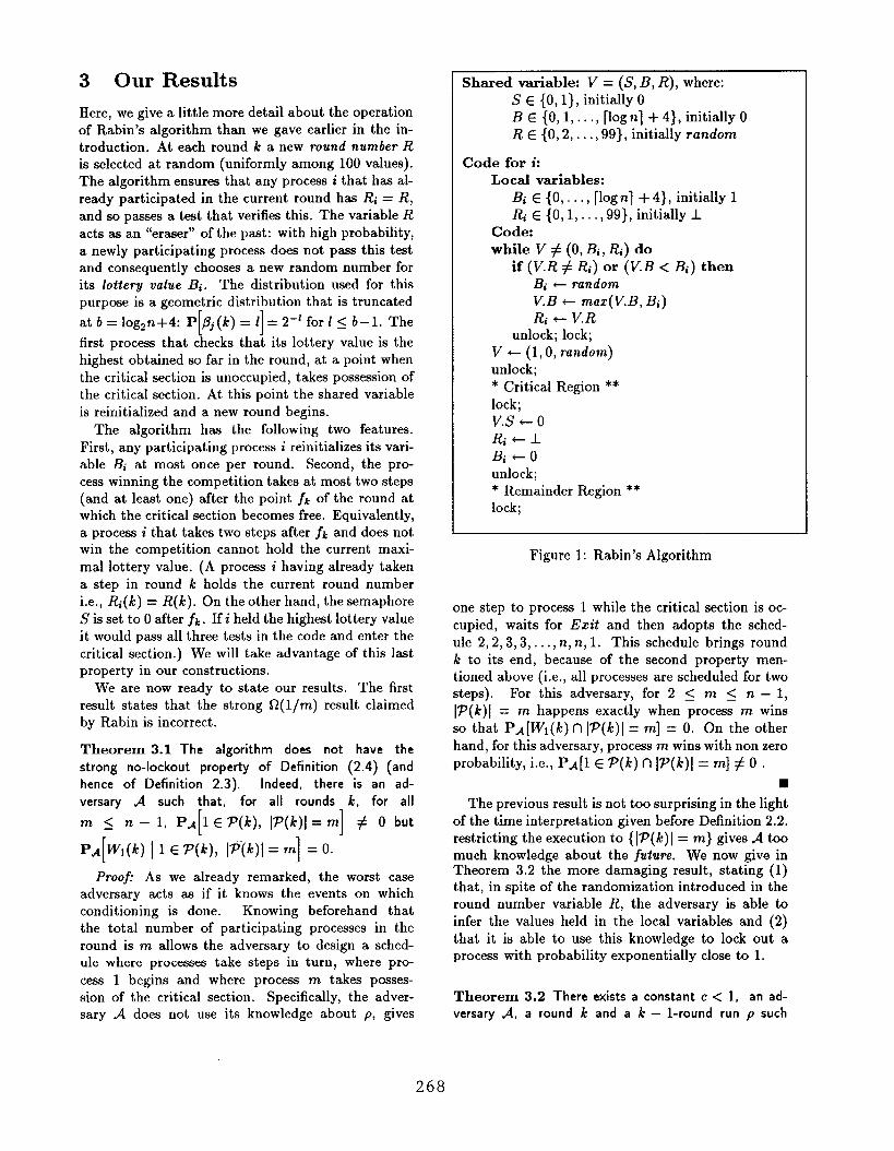
appears in Figure 1.

We begin our analysis by presenting three differ-

ent formal versions of the no-lockout property. These

three statements are of the form discussed in the in-

troduction and give lower bounds on the (conditional)

probability that a participating process wins the cur-

rent round of competition. They differ by the nature

of the events involved in the conditioning and by the

values of the lower bounds.

Described in this formal style, the strong no-

lockout property claimed by Rabin involves condi-

tioning over m, the number of participating processes

in the round. We show in Theorem 3.1 that the ad-

2In the statement of this property, a” trying round” refers tothe interval b.tw..n tm.o successive allocations of the resource,

and the “critical region” refers to the interval during which aparticular process has the resource allocated to it. A “criticalregion” is also called a “critical section”.

versary can use this fact in a simple way to lock out

any process during any round.

On the other hand, the weak c/n no-lockout prop-

ert y that was claimed for Ben-Or’s algorithm involves

only conditioning over events that describe the knowl-

edge of the adversary at the end of previous round.

We show in Theorems 3.2 and 3.4 that the algorithm

suffers from a different flaw which bars it from satis-

fying even this property.

We discuss here informally the meaning of this re-

sult. The idea in the design of the algorithm was to

incorporate a mathematical procedure within a dis-

tributed context. This procedure allows one to se-

lect with high probability a unique random element

from any set of at most n elements. It does so in

an efficient way using a distribution of small support

(“small” means here O(log n)) and is very similar

to the approximate counting procedure of [3]. The

mutual exclusion problem in a distributed system is

also about selecting a unique element: specifically the

problem is to select in each trying round a unique

process among a set of competing processes. In order

to use the mathematical procedure for this end and

select a true random participating process at each

round and for all choices of the adversary, it is neces-

sary to discard the old values left in the local variables

by previous calls of the procedure. (If not, the adver-

sary could take advantage of the existing values.) For

this, another use of randomness was designed so that,

with high probability y, at each new round, all the par-

ticipating processes would erase their old values when

taking a step.

Our results demonstrate that this use of random-

ness did not actually fulfill its purpose and that the

adversary is able in some instances to use old lottery

values and defeat the algorithm.

In Theorem 3.5 we show that the two flaws re-

vealed by our Theorems 3.1 and 3.2 are at the center

of the problem: if one restricts attention to execu-

tions where program variables are reset, and if we

disallow the adversary to use the strategy revealed by

Theorem 3.1 then the strong bound does hold. Our

proof highlights the general difficulties encountered

in our methodology when attempting to disentangle

the probabilities from the influence of A.

The algorithm of Ben-Or which is presented at the

end of [6] is a modification of Rabin’s algorithm that

uses a shared variable of constant size. All the meth-

ods that we develop in the analysis of Rabin’s al-

gorithm apply to this algorithm and establish that

Ben-Or’s algorithm is similarly flawed and does not

satisfy the l/2en no-lockout property claimed for it

in [6]. Actually, in this setting, the shared variables

can take only two values, which allows the adversary

to lock out processes with probability one, as we show

265

in Theorem 3.8,

In a recent paper [7], Kushilevitz and Rabin use our

results to produce a modification of the algorithm,

solving randomized mutual exclusion with log22n val-

ues. They solve the problem revealed by our The-

rem 3.1 by conducting before round k the competition

that results in the control of Crit by the end of round

k. And they solve the problem revealed by our The-

orem 3.2 by enforcing in the code that the program

variables are reset to O.

The remainder of this paper is organized as follows.

Section 2 contains a description of the mutual exclu-

sion problem and formal definitions of the strong and

weak no-lockout properties. Section 3 contains our

results about the n~lockout properties for Rabin’s

algorithm. It contains Theorems 3.1 and 3.2 which

disprove in different ways the strong and weak n-

lockout properties and Theorem 3.5 whose proof is

is a model for our methodology: a careful analysis of

this proof reveals exactly the origin of the flaws stated

in the two previous theorems. One of the uses of ran-

domness in the algorithm was to disallow the adver-

sary from knowing the value of the program variables.

Our Theorems 3.2 and 3.7 express that this objective

is not reached and that the adversary is able to in-

fer (partially) the value of all the fields of the shared

variable. Theorem 3.8 deals about the simpler setting

of Ben-Or’s algorithm.

Some mathematical properties needed for the con-

structions of Section 3 are presented in an appendix

(Section 4).

2 The Mutual Exclusion Prob-

lem

The problem of mutual exclusion is that of continu-

ally arbitrating the exclusive ownership of a resource

among a set of competing processes. The set of com-

peting processes is taken from a universe of size n and

changes with time. A solution to this problem is a

distributed algorithm described by a program (code)

C having the following properties. All involved pro-

cesses run the same program C. C is partitioned into

four regions, Try, Crit, Exit, and Rem which are

run cyclically in this order by all processes executing

C. A process in Crit is said to hold the resource. The

indivisible property of the resource means that at any

point of an execution, at most one process should be

in Crit.

2.1 Definition of Runs, Rounds, and

Adversaries

In this subsection, we define the notions of run, round,

adversary, and fair adversary which we will use to

define the properties of progress and no-lockout.

A run p of a (partial) execution E is a se-

quence of triplets {(pl, oldl, newl), (pz, oldz, newz),

. . . (p,, old,, newt) . ..} indicating that process p,

takes the tth step in & and undergoes the region

change oldt ~ ne wi during this step (e.g., oldt =

newt = Try or old: = Try and newt = Grit). We

say that 8 is compatible with p.

An admissible adversary for the mutual exclusion

problem is a mapping A from the set of finite runs

to the set {l,..., n} that determines which process

takes its next step as a function of the current par-

tial run. That is, the adversary is only allowed to

see the changes of regions. For every t and for ev-

ery run p = {(P1, o~dl, ne~l), (PZ, old2., newz),.. .},

A[{(P1, o~dl, newl),... , (Pt, oldt, newt)}] = pt+l. Wethen say that p and d are compatible.

An adversary d is fair if for every execution, every

process i in Try, Crit, or Ezit is eventually provided

by A with a step. This condition describes “normal”

executions of the algorithm and says that processes

can quit the competition only in Rem.

A round of an execution is the part between two

successive entrances to the critical section (or before

the first entrance). Formally, it is a maximal execu-

tion fragment of the given execution, containing one

transition Try - Crit at the end of this fragment

and no other transition Try -+ Crit. The round of a

run is defined similarly.

A process i participates in a round if i takes a step

while being in its trying section Try.

2.2 The Progress and No-Lockout

Properties

Definition 2.1 An algorithm C that solves mutual ex-

clusion guarantees progress if, for all fair adversaries,

there is no infinite execution in which, from some point

on, at least one process is in its Try region (respec-

tively its Exit region) and no transition Try ~ Crit

(respectively Exit ~ Rem) occurs.

The properties that we considered thus far are non-

probabilistic. The no-lockout property is probabilis-

tic. Its formal definition requires the following nota-

tion:

Let X denote any generic quantity whose value

changes as the execution unfolds (e.g., a program

variable). We let X(k) denote the value of X just

prior to the last step (Try ~ Crit) of the kth round

of the execution. As a special case of this general

not ation, we define the following.

266

P(k) is the set of participating processes in round

k. (Set ?(k) = 0 if $ has fewer then k rounds.) The

notation ~(k) is consistent with the general notation

because the set of processes participating in round k is

updated as round k progresses: in effect the definition

of this set is complete only at the end of round k (this

fact is at the heart of our Theorem 3.1).

t(k) is the total number of steps that are taken by

all the processes up to the end of round k.

N(k) is the set of executions in which all the pro-

cesses j participating in round k reinitialize their pro-

gram variables Bj with a new value ~j (k) during

round k. (~ stands for New-values.) /3~(k); k =

1,2,..., j = 1, . . . . n is a family of iid 3 random

variable whose distribution is geometric truncated at

log,n + 4 (see [6]).

For each i and k, we let Wi(k) denote the set of

executions in which process i enters the critical region

at the end of round k.

We consistently use the probability theory conven-

tion according to which, for any property S, the set

of executions {$ : $ has property S} is denoted aa

{S}. Then:

For each step number t and each execution t

we let nt(~) denote the run compatible with the

first t steps of ~. For any t-steps run p, {~t = p}

represents the set of executions compatible with

P. ({ret = p} = @if p has fewer then i! steps.) We

will use ~k in place of ~~(~) to Simplify notation.

Similarly, for all m < n, { lP(k) I = m} repre-

sents the set of executions having m processes

participating in round k.

The quantities N(k), {n, = p}, Wi(k), {l’P(k)/ =

m} are sets of executions: for a given adversary they

are random events in the probability space of random

executions endowed with the measure dPA.

We now present the various no-lockout properties

that we want to study. A first question is to char-

acterize relevant events I over which conditioning

should be done. Note first that restricting the set

of executions to the ones having a certain property

amounts to conditioning on this property. In par-

ticular, we will condition on the fact that process i

participates in round k. A crucial remark is that, in

the worst case adversary framework that we are in-

terested in, the adversary minimizing PA [Wj(k) II]

will make its choices as if “knowing” 1. We will derive

telling consequences from this fact.

We have actually in mind to compute the proba-

bility of Wj (k) at different points Sh of the execution.

3Recall that iid stands for “independent and identically dis-

tributed”.

One way to go, would be to condition on the past

execution. But, by our previous remark, this is tan-

tamount to allow the adversary to this knowledge. It

is then easy to see that lockout is possible. Another

natural alternative that we will adopt, is to compute

the probability at point sk “from the point of view

of the adversary”: this translates formally into con-

ditioning over the value of the run up to point sk.

We will say that such a no-lockout property is rrm-

knowing.

The first two definitions involve evaluating the

probabilities “at the beginning of round k“.

Definition 2.2 (Weak, Run-knowing, Proba-

bilistic no-lockout ) A solution to the mutual exclu-

sion problem satisfies weak, run-knowing probabilistic

no-lockout whenever there exists a constant c such that,

for every fair adversary A, every k >1, every (k – l)-

round run p compatible with A, and every process i,

P~[W~(k) I ~k-~ = ~, i E P(k)] > C/71,

whenever PA[~k-1 = p, i E P(k)] # O .

The next property formally expresses statement (*)

of Rabin. As we mentioned in our general presenta-

tion, considering rounds having m participating pr~

cesses corresponds to conditioning on this fact.

Definition 2.3 (Strong, Run-knowing, Proba-

bilistic no-lockout ) The same as in Definition 2.2

except that:

PA[~~(k) I ~k-1 = p, i G P(k), lP(k)l = m] ~ c/m,

whenever PA[~k-l = p, i c P(k), lP(k)l = m] # O .

Recalling the two interpretations of conditioning in

terms of time and knowledge held by the adversary,

we see that this property differs fundamentally from

the previous one because, here, the adversary is pro-

vided with the number of processes due to participate

in the future round (i.e., after t(k – l)). By integra-

tion over m, we see that an algorithm satisfying the

strong property also satisfies the weak property.

The next definition is the transcription of the pre-

vious one for the case where the probability is “com-

puted at the beginning of the execution” (i.e., sk = O

for all k).

Definition 2.4 (Strong, Without knowledge,

Probabilistic no-lockout ) The same as in Defini-

tion 2.2 except that:

P~[Wi(k) \ i c P(k), lP(k)l = m] z c/m,

whenever PA[i c P(k), ]P(k)l = m] # O .

By integration over p we see that an algorithm hav-

ing the property of Definition 2.3 is stronger then one

having the property of Definition 2.4. Equivalently,

an adversary able to falsify Property 2.4 is stronger

then one able to falsify Property 2.3.

267

3 Our Results

Here, we give a little more detail about the operation

of Rabin’s algorithm than we gave earlier in the in-

troduction. At each round k a new round number R

is selected at random (uniformly among 100 values).

The algorithm ensures that any process i that has al-

ready participated in the current round has Ri = R,

and so passes a test that verifies this. The variable R

acts aa an “eraser” of the past: with high probability,

a newly participating process does not pass this test

and consequently chooses a new random number for

its lottery value Bi. The distribution used for this

purpose is a geometric distribution that is truncated

at b = logzn+A: P[~j(k) = I]= 2-’ for 1 ~ b–1. The

first process that checks that its lottery value is the

highest obtained so far in the round, at a point when

the critical section is unoccupied, takes possession of

the critical section. At this point the shared variable

is reinitialized and a new round begins.

The algorithm has the following two features.

First, any participating process i reinitializes its vari-

able Bi at most once per round. Second, the pro-

cess winning the competition takes at most two steps

(and at least one) after the point fk of the round at

which the critical section becomes free. Equivalently,

a process i that takes two steps after fk and does not

win the competition cannot hold the current maxi-

mal lottery value. (A process i having already taken

a step in round k holds the current round number

i.e., Ri(k) = R(k). On the other hand, the semaphore

S is set to O after fk. If i held the highest lottery value

it would pass all three tests in the code and enter the

critical section. ) We will take advantage of this last

property in our constructions.

We are now ready to state our results. The first

result states that the strong f2(l/rn) result claimed

by Rabin is incorrect.

Theorem 3.1 The algorithm does not have the

strong no-lockout property of Definition (2.4) (and

hence of Definition 2.3). Indeed, there is an ad-

versary A such that, for all rounds k, for all

m g n – 1, P~[l c P(k), lP(k)l = m] # O but

P~[Wl(k) \ 1 c ‘P(k), I?(k)l = m] = O.

Proofi As we already remarked, the worst case

adversary acts as if it knows the events on which

conditioning is done. Knowing beforehand that

the total number of participating processes in the

round is m allows the adversary to design a sched-

ule where processes take steps in turn, where pro-

cess 1 begins and where process m takes posses-

sion of the critical section. Specifically, the adver-

sary A does not use its knowledge about p, gives

Shared variable: V = (S, B, R), where:

S E {O, 1}, initially O

BE{ O,l,..., [log nl + 4}, initially O

R E {0,2, . . . . 99}, initially random

Code for i:

Local variables:

Bi~{07... Y[log nl + 4}, initially 1

Ric{o,l,.. ., 99}, initially 1

Code:

while V # (O, Bi, ~) do

if (V.R # ~) or (V.B < Bi) then

Bi - random

V.B + maz(V.B, Bi)

& t V.R

unlock; lock;

V t (1, O, random)

unlock;

* Critical Region **

lock;

V.s + c1

Ri+l

Bi-o

unlock;

* Remainder Region **

lock;

Figure 1: Rabin’s Algorithm

one step to process 1 while the critical section is oc-

cupied, waits for Exit and then adopts the sched-

ule 2,2, 3,3,..., n, n, 1. This schedule brings round

k to its end, because of the second property men-

tioned above (i.e., all processes are scheduled for two

steps). For this adversary, for 2 s m ~ n – 1,

l~(k)l = m happens exactly when process m wins

so that P~[W1(k) n /P(k)l = m] = O. On the other

hand, for this adversary, process m wins with non zero

probability, i.e., PA[l E P(k) n lP(k)l = m] # O .

9

The previous result is not too surprising in the light

of the time interpretation given before Definition 2,2.

restricting the execution to { lP(k) I = m} gives A too

much knowledge about the fuiu~e. We now give inTheorem 3.2 the more damaging result, stating (1)

that, in spite of the randomization introduced in the

round number variable R, the adversary is able to

infer the values held in the local variables and (2)

that it is able to use this knowledge to lock out a

process with probability exponentially close to 1.

Theorem 3.2 There exists a constant c < 1, an ad-

versary A, a round k and a k – l-round run p such

268

that:

P~[PVI(k) I 7r~-I = p, 1 G P(k)] < e-32 + c“,

We need the following definition in the proof,

Definition 3.1 Let 1 be a round. Assume that, during

round 1, the adversary adopts the following strategy. It

first waits for the critical section to become free, then

gives one step to process j and then two steps (in any

order) to s other processes. (We will call these test-

processes.) Assume that at this point the critical section

is still available (so that round 1 is not over). We then

say that process j is an s-survivor (at round /).

The idea behind this notion is that, by manufactur-

ing survivors, the adversary is able to select processes

having high lottery values. We now describe in more

detail the selection of survivors and formalize this last

fact,

In the following we will consider an adversary con-

structing sequentially a family of s-survivors for the

four values s = 2]0gzn+~; t = –1, . . . . –5. When-

ever the adversary manages to select a new survivor

it stores it, i.e, does not allocates it any further step

until the selection of survivors is completed. (A ac-

tually allocates steps to selected survivors, but only

very rarely, to comply with fairness. Rarely means

for instance once every nT2 steps, where T is the ex-

pected time to select an n/2-survivor.) By doing so,

A reduces the pool of test-processes still available.

We assume that, at any point in the selection pro-

cess, the adversary selects the test-processes at ran-

dom among the set of processes still available. (The

adversary could be more sophisticated then random,

but this is not needed.) Note that a new s-survivor

can be constructed with probability one whenever the

available pool has size at least s + 1: it suffices to re-

iterate the selection process until the selection com-

pletes successfully.

Lemma 3.3 There is a constants d such that for any

t = –5,..., –1, for any 2’Ogzn+~-survivor j, for any

Q=(), ...,5

PA[Bj (/) = Iogn + t + a] ~ d.

Proof: Let s denote logn + t. Let j be an s-survivor

and il, iz,. ... si be the test-processes used in its se-

lection. Assume also that j drew a new value l?j (1) =

Bj (1) (this happens with probability gl = .99 .) Re-

mark that Bj(i) = Max{l?il (1),.. ., Bi, (/), Bj (i)}: if

this were not the case, one of the test-processes would

have entered Crit. As the test processes are selected

at random, each of them has with probability .99 a

round number different from R(r) and hence draws a

new lottery number @j (i). Hence, with high proba-

bility q2 >0, 90’% of them do so. The other of them

keep their old lottery value Bj (1 – 1): this value, be-

ing old, has lost in previous rounds and is therefore

stochastically smaller 4 then a new value ~j ({). (An

application of Lemma 4.5 formalizes this.) Hence,

with probability at least qlqz we have the following

stochastic inequality:

Max{/31(1) ,... ,Ps.9rl,loo}

<c Bj(i) <z Max{/31(Z), . . . ,/38+1(1)}.

Corollary 4.4 then shows that, for a = 0,...,5, with

probability at least q1q2, PA [Bj (1) = logzs] ~ q3 for

some constant q3 (q3 is close to 0.01). Hence, with

probability at least d ~f q1q2q3, Bj (1) is equal to

log@ + 0,. ■

Proof of Theorem 3.2: The adversary uses a prepa-

ration phase to select and store some processes hav-

ing high lottery values. We will, by abuse of lan-

guage, identify this phase with the round p which

corresponds to it. When this preparation phase isover, round k begins.

Preparation phase p: For each of the five values

log2n+t, t= –5, . . . . – 1, A selects in the preparation

phase many (“many” means n/20 for t = –5, ....–2

and 6n/20 for i! = —1) 21°gzn+t-survivors. Let sl de-

note the set of all the survivors thus selected. (Note

that lS1 [ = n/2 so that we have enough processes

to conduct this selection). By partitioning the set

of 210gzn- l-survivors into six sets of equal size, for

each of the ten values t = –5, . ...4, A has then se-

cured the existence of n/20 processes whose lottery

value is logzn + t with probability bigger then d. (By

Lemma 3.3.)

Round k: While the critical section is busy, A gives

a step to each of the n/2 processes from the set S2

that it did not select in phase p. When this is done,

with probability at least 1 – 2-32 (see Corollary 4.2)

the program variable B holds a value bigger or equal

then log2n – 5. The adversary then waits for the

critical section to become free and gives steps to the

processes of S1 it selected in phase p. A process in

S2 can win access to the critical section only if the

maximum lottery value Bsz ‘=i Max, ● ~z Bj of all

the processes in S2 is strictly less then log2n – 5 or if

no process of S1 holds both the correct round number

R(k) and the lottery number Bs,. This consideration

gives the bound predicted in Theorem 3.2 with c =

(1 – d/100)1/20. ■

Our proof actually demonstrates that there is an

adversary that can lock out, with probability expo-

nentially close to 1, an arbitrary set of n/2 processes

4 A real random variable X is st .chasti.ally smaller then

another one Y (we write that: X <~ Y) exactly when, for all

z c R, P[X > Z] < P[Y ~ z]. Hence, if X < Y in the usualsense, it is also stochastically smaller.

269

during some round. With a slight improvement we

can derive an adversary that will succeed in lock-

ing out (with probability exponentially close to 1)

a given set S3 of, for example, n/100 processes at all

rounds: we just need to remark that the adversary can

do without this set S3 during the preparation phase

p. The adversary would then alternate preparation

phases pl, p2, . . . with rounds kl, k2, . . . The set S3

of processes would be given steps only during rounds

kl, kz,. . . and would be locked out at each time with

probability exponentially close to 1.

In view of our counterexample we might think that

increasing the size of the shared variable might yield

a solution. For instance, if the geometric distribu-

tion used by the algorithm is truncated at the value

b = 2 logzn instead of log2n + 4, then the adversary

is not able as before to ensure a lower bound on the

probability that an n/2-survivor holds b as its lot-

tery value. (The probability is given by Theorem 4.1

with z = logn.) Then the argument of the previ-

ous proof does not hold anymore. Nevertheless, the

next theorem establishes that raising the size of the

shared variable does not help as long aa the size stays

sub-linear. But this is exactly the theoretical result

the algorithm was supposed to achieve. (Recall the

n-lower bound of [1] in the deterministic case.) Fur-

thermore, the remark made above applies here also:

a set of processes of linear size can be locked out at

each time with probability arbitrarily close to 1.

Theorem 3.4 Suppose that we modify the algorithm

so that the set of possible round numbers used has size

r and that the set of possible lottery numbers has size

b (log2n + 4 < b ~ n). Then there exists positive

constants c1 and C2, an adversary A, and a run p such

that

PA[~~(k) I m~_I = p, 1 e P(k)] <

Proof: We consider the adversary A described in

the proof of theorem 3.2: for t = –5, . . . . –2, A pre-

pares a set Ti of 210gzn+t-survivors, each of size n/20,

and a set T_ 1 of 210Qn - l-survivors; the size of T_ 1 is

6/20n. (We can as before think of this set as being

partitioned into six different sets.) We let q stand for

6/20 in the sequel.

Let pi denote the probability that process 1 holds I

as its lottery value after having taken a step in round

k. For any process j in S_ ~ let also ql denote the

probability that proc~ss j holds 1 as its-lottery

at the end of the preparation phase p.

The same reasoning as in Theorem 3.2 then

to the inequality:

PA[~~(k) I ~~-~ = p, 16 P(k)] ~

value

leads

e ’32 +(1 – e-32)(1 – d/r)n/20

+ ~ Pl(l – ;)’r”.

l~10gzn+5

Write 1 = log2n + z – 1 = log2(n/2) + Z. Then, aa

is seen in the proof of Corollary 4.4, qr = e_2M21-(

for some ~ ~ (x, z+ 1). For 1 ~ log2n+5, z is at least6 and e-2x-< W 1 so that qi _ zl-~ > 21-Z. on the

—

other hand pl = 2-1 = 2-Z+l/n.

Define ~(z) ~f e-2 ‘-’vn/r so that @l(z) =

e- 2’-=’rnlr21-xqn/r. Then:

~ Pm(l - Y)”” < 2/n~2-2(1 - =)””Q10g2+5 z~6

~ 2/n ~ 2-”e–t~onJ

z~6

= l/n ~ 21-ze-(~~”)

x26

=+ X4’(4

x>6

<~ /“ @’(z)dzrp2 ~

= + [W?

= -_&l _ e-2-40n/~]

< J-.r,m2

■

To simplify the notations in the sequel, we will let

il, ..., ipy~)l denote the elements of P(k). And we

will let pl, pz, . . . denote the sequence of processes

taking steps in turn during round k: recall that a

process i can take several steps during the round.

The flaw of the protocol revealed in Theorem 3.2 is

based on the fact that the variable R does not act as

an eraser of the past and that the adversary can use

old values to defeat the algorithm. The flaw exhibited

in Theorem 3.1 is based on the fact that, even when

the old values are erased, the algorithm is sensitive to

the order PI, PZ, . . . in which participating procesaea

are scheduled. The adversary can play on this order

in two different ways. It can act on the fact that dif-

ferent scheduling strategies influence in different ways

the size m of the set P(k) (Strategy 1). And it can

use the fact that, for a given number m of participat-

ing processes, the mathematical distribution of the

sequence (@i (k); i E P(k)) is (a priori) sensitive to

the ordering PI, PZ, . . . (Strategy 2). The adversary of

Theorem 3.1 specifically used strategy 1.

The next result shows that the two flaws exhibited

in Theorems 3.1 and 3.2 are at the core of the prob-

270

lem: the algorithm does have the strong no-lockout

property when we precondition on the fact that the

internal variables of the participating processes are

reset to new values and when we bar the adversary

from using strategy 1. We will actually prove this re-

sult for a slightly modified version of the algorithm.

Recall in effect that the code given in Page 6 is opti-

mized by making a participating process i draw a new

lottery number when it is detected that V.B < Bi.

We will consider the “de-optimized” version of the

code in which only the test V.R # Ri ? causes of a

new drawing to occur.

The next definition formalizes the restriction that

we impose on the adversary, It says that the adver-

sary commits itself to the value of ?(k) at the” begin-

ning of round k.

Definition 3.2 We say that an adversary is restricted

when, for each round, it allocates a step to all participat-

ing processes (of this round) before the critical section

becomes free. We will let d’ (as opposed to d) denote

any such adversary.

We will make constant use of the notation [n] ~’

{1,2,..., n}. Also, for any sequence (Uj )j EN we will

write ai = Umaxai to mean that i is the only indexjEJ

in J for which CZi= Mea? Uj.

Theorem 3.5 For every process i = 1, . . . . n, for ev-

ery round k ~ 1, for every restricted adversary A’ and

for every (k – 1)-round run p compatible with A’,

LPA, [Wi(k) N(k), ~k-l = ~, i c P(k), I’P(k)l = m]

~ ~, whenever

P~, [N(k), m~_l = p, i ~P(k), Ip(k)l = m] # O

Proof:

We first define the events U(k) and U; (k), where

is any subset of {1, . . ..n}.

U(k) ~f {3!i G P(k) s.t. Bi(k) = ,Nll;, Bj(k):

J

The main result established in [6] can formally be

restated as:

Vm s n, P[ U(~l (k)] ~ 2/3. (1)

Following the general proof technique described in the

introduction we will prove that :

P~,[U(k) I ~(k), Tk_l = p, i E P(k), lP(k)l = m]

P[U~(k)] , and that:

P~,[W~(k) I ~(k), mk_l = p, i G P(k), lP(k)l = m, U(k)]

= P[fl:(k) = ~ax Pj(k) I LL(k) ] .

The events involv~d ;~]the LHS of the two inequal-

ities (e.g., Wi(k), U(k), {lP(k)l = m}, {r~._l = p},

{i E P(k)}) depend on A’ whereas the events involved

in the RHS are pure mathematical events over which

A’ has no control.

We begin with some important remarks.

(1) By definition, the set P(k) = {il, i2, . ..} is

decided by the restricted adversary A’ at the begin-

ning of round k: for a given A’ and conditioned on

{m~-.I = p}, the set P(k) is defined deterministically.

In particular, for any i, P~, [ i G P(k) I Tk.l = ~]

has value O or 1. Similarly, there is one value

m for which PAl[lP(k)l = m I ~k_l = p] = 1 .

Hence, for a given adversary A’, if the random event

{~(k), m~-l = p, i ~ P(k), lP(k)l = m} has

non zero probability, it is equal to the random event

{N(k), mk_l=p}~’1.

(2) Recall that, in the modified version of the

algorithm that we consider here, a process i draws a

new lottery value in round k exactly when Ri(k _ 1) #

R(k). Hence, within 1, the event Af(k) is equal to

{Ri,(k - 1) # R(k), . . . . Ri~(k – 1) # R(k)}. On the

other hand, by definition, the random variables (in

short r.v.s) flij; ij E P(k) are iid and independent

from the r.v. R(k). This proves that, (for a given

A’), conditioned on {m_l = p}, the r,v. N(k) is

independent from all the r.v.s ~i,. Note that U$,(k.(k)

is defined in terms of (i.e., measurable with respect

to) the (pi,; ij E P(k)), so that U$(k)(k) and ~(k)are also independent.

(3) More generally, consider any r.v. X defined

in terms of the (/?ij; ij E P(k)): X = f(@i, , . . . . ~i~)

for some measurable function ~. Recall once more

that the number m and the indices il, . . . . im are de-

termined by {~k_ 1 = p} and A’. The r.v.s ~ij being

iid, for a fixed A’, X then depends on {~k_l = p}

only through the value m of lP(k) 1. Formally, this

means that, conditioned on lP(k) 1, the r,v.s X and

{~k_~ = p} are independent: E~,[X I mk_~ = p ]=

EdJ[X I lP(k)l = m] = E[~(~l, . . . ,~~)]. (More pre-

cisely, this equality is valid for the value m for which

PA[m~_l = p , lP(k)l = m] # O,) A special conse-

quence of this fact is that PA~[U&[k)(k) I ~k-1 =

P] = Wfml(k)l.Remark that, in U(k), the event Wi (k) is the same

as the event {Bi (k) = .~emP~~)Bj(k)}. This justifies

the first following equahty. The subsequent ones are

comment ed afterwards. Also, the set 1 that we con-

sider here is the one having a non zero probability

described in Remark (1) above.

PAJ [~i(k) I ~(k), ~]

= P~, [Bi(k) = ~~~~)Bj (k) I U(k), I ]

= PAI [i%(~) = ~em~~y)~j(k) \ ‘$(k)(k)! J 1 (2)

= PA’[~i(k) = ~~~~)~j(k) \ U$(~)(k), ‘k-l ~?)

271

Equation 2 is true because we condition on N(k)

and because U(k) n N(k) = U&(k)(k). Equation 3 is

true because N(k) is independent from the r.v.s ~~j

as is shown in Remark (2) above.

We then notice that the events {pi(k) =

~<m~~f)% (k)} and U&(k)(k) (and hence their intersec-

tion) are defined in terms of the r.v.s ~i j. From re-

mark (3) above, the value of Eq. 3 depends only on

m and is therefore independent of i. Hence, for all i

and j in ?(k), P4J[~i(k) I U(k), I ] = PA~[Wj(k) I

U(k), 1].

On the other hand, ~iEp(k)pA’~i(k) =

yY;@(k) I Z&k](k), m~-1 = p ] = 1: indeed,

one of the /?i, has to attain the maximum.

These last two facts imply that, Vi E P(k),

P4,[~i(k) I U(k), 1 ] = l/m.

We now turn to the evaluation of P4J[U(k) I l].

pA/[ U(k) I I ] = PAJ[ ~$(k)(k)\ ~1 (4)

= PA’[ U$(~)(k) I ‘~-l = P 1 (5)

= p[~(ml(k)l2 2/3 . (6)

Equation 4 is true because we condition on N(k).

Eq. 5 is true because U&(k)(k) and Af(k) are indepen-

dent (See Remark (2) above). The equality of Eq. 6

stems from Remark (3) above and the inequality from

Eq. 1.

We can now finish the proof of Theorem 3.5.

■

We discuss here the lessons brought by our results.

(1) Conditioning on N(k) is equivalent to force the

algorithm to refresh all the variables at each round.

By doing this, we took care of the undesirable linger-

ing effects of the past, exemplified in Theorems 3.2

and 3,4. (2) It is not true that:

i.e., that the adversary has no control over the event

{~i (k)= ,~~k)~j (~)}. (This was Rabin’s statement

in [6].)

Indeed, the latter probability is equal to l/m

whereas we proved in Theorem 3.1 that there is an

adversary for which the former is O when m ~ n – 1.

The crucial remark explaining this apparent para-

dox is that, implicit in the expression P4~i(k) =

,hll,)3j (k) I . . .], is the fact that the random vari-

ables /?j (k) (for j E P(k)) are compared to each other

in a specific way decided by A, before one of them

reveals itself to be the maximum. For instance, in

the example constructed in the proof of Theorem 3.1,when j takes a step, @j(k) is compared d~ to the

@/(k); 1 S j, and the situation is not symmetricamong the processes in P(k).

But, if the adversary is restricted as in our Defi-

nition 3.2, the symmetry is restored and the strong

no-lockout property holds.

Rabin and Kushilevitz used these ideas from our

analysis to produce their algorithm [7].

In our last Theorem 3.5 we used the restriction on

the adversary A’ mostly to derive a l/m bound. If we

consider a general adversary A it is interesting to note

that we can still ensure the weak lockout-property:

Theorem 3.6 For every process i = 1,..., n, for ev-

ery round k > 1, for every adversary A and for every

(k - 1)-round run p compatible with A,

P4[~i(k) I Af(k)l fi~-l = ~, i E P(k)] ~ l/n,

whenever P4[ N(k), r~-l = p, i G P(k)] # O .

Proofi Omitted. ■

This theorem holds also if, as in the context of the-

orem 3.4, the algorithm uses b lottery numbers. This

shows that the result of Theorem 3.6 is not trivial: in-

deed, when b = 210g2, the probability P~i(k) = b] of

drawing the highest possible number is a o(l/n), One

of the difficulties of the proof is that the apparently

innocuous event {i G ?(k)} is in the future of the

point t(k – 1) at which the probability is estimated:

the adversary could conceivably also use this fact to

ensure some specific values of the variables when i

participates.

Our Theorems 3.1, 3.2 and 3.4 explored how the

adversary can gain and use knowledge of the lottery

values held by the processes. The next theorem states

that the adversary is similarly able to derive some

knowledge about the round numbers, contradicting

the claim in [6] that “because the variable R is ran-

domized just before the start of the round, we have

with probability 0.99 that E. # R.” Note that, ex-pressed in our terms, the previous claim translates

into R(k) # &(k – 1).

Theorem 3.7 There exists an adversary A, a round k,

a step number t,a run pt, compatible with A, having t

steps and in which round k is under way such that

P4[R(k) + Rl(k – 1) I mt = p~] <.99.

Proof:

272

We will write pt = p’p where p’ is a k – l-round run

and p is the run fragment corresponding to the kth

round under way. Assume that p’ indicates that, be-

fore round k, processes 1,2,3,4 participated only in

round k – 1, and that process 5 never participated be-

fore round k. Furthermore, assume that during round

k – 1 the following pattern happened: d waited for

the critical region to become free, then allocated one

step in turn to processes 2, 1, 1,3, 3,4,4; at this point

4 entered the critical region. (All this is indicated in

p’.) Assume also that the partial run p into round k

indicates that the critical region became free before

any competing process was given a step, and that the

adversary then allocated one step in turn to processes5,3,3, and that, after 3 took its last step, the critical

section was still free. We will establish that, at this

point,

PA[R(k) # Ii?l(k – 1) I Tt = p’p] <.99.

By assumption k – 1 is the last (and only) round

before round k where processes 1,2,3 and 4 partic-

ipated. Hence Rl(k – 1) = R2(k – 1) = l?~(k –

1) = R(k – 1). To simplify the notations we will

let R’ denote this common value. Similarly we will

write /3{, /3~, . . . in place of /?l(k – 1), /?2(k – 1),. . .

We will furthermore write /31, BZ,. . . in place of

Pi(k), flz(k), . . . and B, R in place of B(k), R(k).

Using Bayes’ rule gives us:

PA[R# R’ I p’, p]

PA[R# R’ I p’] PA[p I p’, R# R’] (7)=

PA~ I p’]

In the numerator, the first term PA [R # R’ I p’] is

equal to 0.99 because R is uniformly distributed and

independent from R’ and p’. We will use this fact

another time while expressing the value of PA ~ I p’] :

I P’]

PA[p I p’, R # R’] PA[R # R’ I p’]

+PA~l p’, R= R’] PA[R= R’ Ip’]

0.99 PA~ I p’, R# R’] (8)

+0.01 pA~ I P’, R= R’].

● Consider first the case where R # R’. Then pro-

cess 3 gets a YES answer when going through the

test “(V.R # R3) or (V.B < B3)”, and consequently

chooses a new value B3 (k) = ~3. Hence

PA~ I p’, R# R’] = p[~3 < /35]. (9)

● Consider now the case R = Rt. By hypoth-

esis, process 5 never participated in the computa-tion before round k and hence draws a new number

B5(k) = /35, Hence:

PA~ I p’, R= R’] =

P..t[Bdk) < P5 I P’, R= R’]. (lo)

As processes 1, ..., 4 participated only in round

k – 1 up to round k, the knowledge provided by p’

about process 3 is exactly that, in round k -1, pro-

cess 3 lost to process 2 along with process 1, andthat process 2 lost in turn to process 4, i.e., that

~~ < /3~, ~~ < P; and /?~ < ~~. For the sake of no-tational simplicity, for the rest of this paragraph we

let X denote a random variable whose law is the law

of ~~ conditioned on {/3j > Max{/3{, /3j}, /3~ < /3j}.This means for instance that, Vz G R,

1P[x2Z]=+ 2zIP!>Mwc{P{,B:},/%<Pi.When 3 takes its first step within round k, the pro-

gram variable V.B holds the value /3cj. As a conse-

quence, 3 chooses a new value when and exactly when

B3(k – 1)(= flj) is strictly bigger then /35. (The case

~~ =65 would lead 3 to take possession of the criticalsection at its first step in round k, in contradiction

with the definition of p; and the case /3~ < /?5 leads 3

to keep its “old” lottery value B3(k – l).) From this

we deduce that:

l’A[&(k) <P5 I P’, R= R’]=W% cP5 I Pi <x’

+P[pj > /35, P3 < /35 I L% < x]. (11)

Using Lemma 4.5 we derive that:

P[P4 < /35 [ P4 < xl 2 p[/Z < /351.

On the other hand P[/3j < @j] = P[/33 < ~s] because

all the random variables /3~(j), i = 1, . . . . n, j ~ 1 are

iid. Taking into account the fact that the last term

of equation 11 is non zero, we have then established

that:

PA[B3(k) < /35 I p’, R = R’] > p[p3 < /35]. (12)

Combining Equations 9, 10 and 12 yields:

PA~ \ p’, R= R’] > PA[p I p’, R# R’].

Equation 8 then shows that PA~ I p’] > PA~ I

p’, R # R’]. Plugging this result into Equation 7

finishes the proof. ■

We finish with a result showing that all the prob-

lems that we encountered in Rabin’s algorithm carry

over for Ben-Or’s algorithm. Ben-Or’s algorithm iscited at the end of [6]. The code of this algorithm is

the same as the one of Rabin with the following mod-ifications. All variables l?, R, Eli, Ri; 1 ~ i ~ n are

273

boolean variables, initially O. The distribution of the

lottery numbers is also different but this is irrelevant

for our discussion.

We show that Ben-Or’s algorithm does not satisfy

the weak no-lockout property of Definition 2.2. The

situation is much simpler then in the case of Rabin’s

algorithm: here all the variables are boolean so that

a simple reasoning can be worked out.

Theorem 3.8 (Ben Or’s Alg.) There is an adver-

sary A, a step number t and a run pi compatible with

A such that

+’Vz(k) I ~t = ~t, 2EP(k)]=o.

Proof: Assume that we are in the middle of round

3, and that the run pt indicates that (at time O the

critical section was free and then that) the schedule

12 233 was followed, that at this point 3 entered in

Crit, that it left Crit, that at this point the schedule

4 1 1 55 was followed, that 5 entered and then left

Crit, that 644 then took a step and that at this

point Crit is still free.

Without loss of generality assume that the round

number R(l) is O. Then R2(1) = O, 111(1) = 1 and

B2 (1) = O: if not 2 would have entered in Crit. In

round 2 it then must be the case that R(2) = 1.Indeed if this was not the case then 1 would have en-

tered the critical section. It must then be the case

that B1(2) = O and B4(2) = 1. And then that

B6 (3) = 1 and R(3) = O: if this was not the case

then 4 would have entered in Crit in the 3rd round.

But at this point, 2 haa no chance to win if sched-

uled to take a step! ■

Acknowledgments I am deeply indebted to

Nancy Lynch who suggested the problem and who

constantly assisted me: this paper is hers too.

References

[1] Burns J., Fischer M., Jackson P., Lynch N. and

Peterson G. Data requirements for implementationof n- process mutual exclusion using a single shared

variable. Journal of the ACM, 29:183-205, (1982).

[2] E. Dijkstra. Solution of a Problem in Concur-

rent Programming Control. Communications ofthe ACM, 321, (1966).

[3] Flajolet P. and Martin N. Probabilistic Count-ing Algorithms for Data Base Applications. Jour-

nal of Computer and System Sciences, 31:182–209,

(1985).

[4] Graham R, and Yao A. On the Improbability of

Reaching Byzantine Agreements Proc. 21st ACM

Symp. on Theory of Computer Science 467-478

(1989).

[5] Hart S., Sharir M. and Pnueli A. Termination of

Probabilistic Concurrent Programs ACM Trans-

actions on Programming Languages and Systems,

Vol 5, Num 3:356-380, (1983).

[6] Michael Rabin. N-process mutual exclusion withbounded waiting by 4 log N- shared variable. Jour-

nal of Computation and System Sciences, 25:66–75

(1982).

[7] Rabin M. and Kushilevitz E. Randomized Mutual

Exclusion Algorithm Revisited This proceedings

[8] Saias I. and Lynch N.

bin’s Randomized Mutual

MIT/L es/TM-462 (1991).

4 Appendix

An Analysis of Ra-

Exclusion Algorithm.

Theorem 4.1 and its corollaries are used in the con-

struction of the adversary in Theorem 3.2 and The-

orem 3.4. Lemma 4.5 is used mostly in the proof of

Theorem 3.7. The proofs can be found in [8].

Definition 4.1 For any sequence (a~)i~N we denote

Max~ai ~’ Max{al, a.2, . . .,a, }.

In this section the sequence (pi) is a sequence of iid

geometric random variables:

Pwi=l] ‘~; l=l,2,...

The following results are about the distribution of the

extremal function Max$@i. The same probabilistic

results hold for iid random variables (~~), having the

truncated distribution used by Rabin: we just need to

truncate at log2rz + 4 the random variables pi and the

values that they take. This does not affect the proba-

bilities because, by definition, P[/3~(k) = log2n + 4 =

‘E10g2n+4 ‘[Pi = ~].

Theorem 4.1 For ~ 1-2 ~ 1/2 we have the following

approximation:

A ~’ P[Max,@i z Iogzs + Z] N 1 – e-2’-= .

A – e-2’-’ < e-2l-z 41-=—.—

s

Corollary 4.2 P[Max,~i ~ Iogzs – 4] ~ 1 – e-32.

Corollary 4.3 P[Max~@i > 10g2S + 8] <0.01.

Corollary 4.4 P[Max,~i = log2s] z 0.17,P[Max,/?i = log2s +/] >0.01, Vl = 1,...,5 .

Lemma 4.5 Let B and A be any real-valued random

variables. Then

Vzc R, PIB~zl B~A]<PIB~z]. 5

5We use the convention that 0/0 = O whenever this quantity

arises in the computation of conditional probabilities.

274