127
UNIVERSIDAD AUTÓNOMA DE MADRID ESCUELA POLITECNICA SUPERIOR PROYECTO FIN DE CARRERA TRANSMISSION OF LAYERED VIDEO CODING USING MEDIA AWARE FEC Nicolás Díez Risueño Junio 2011

UNIVERSIDAD AUTÓNOMA DE MADRID
ESCUELA POLITECNICA SUPERIOR
PROYECTO FIN DE CARRERA
TRANSMISSION OF LAYERED VIDEO CODING USING
MEDIA AWARE FEC
Nicolás Díez Risueño
Junio 2011

i
TRANSMISSION OF LAYERED VIDEO CODING USING MEDIA AWARE FEC
AUTOR: Nicolás Díez Risueño
TUTOR: Cornelius Hellge
PONENTE: José M. Martínez Sánchez
Dpto. de Ingeniería Informática
Escuela Politécnica Superior
Universidad Autónoma de Madrid
Junio de 2011
Multimedia Communications Group
Image Processing Department
Fraunhofer Heinrich-Hertz-Institute
June 2011

ii

iii
Abstract
Current video transmission techniques allow the encoding and transmission of a
video source into a single bit stream over a transmission channel. In such a single stream, a
unique tempo-spatial quality level is transmitted. In this regard, only those clients who
satisfy the stream characteristics are able to receive the video stream.
As an extension of the H.264/AVC standard (Advanced Video Coding), the recently
appeared Scalable Video Coding (SVC) permits the division of a single video stream into
several sub-streams with smaller size and importance. Those sub-streams or layers represent
different quality levels across the overall video stream. In this way, the different quality
levels can be transmitted to different clients with different capabilities within the same bit
stream and adapted in such a way that the media quality can be gracefully degraded with
reception quality instead of a complete signal loss.
Information received through any transmission channel may be affected by losses
due to a number of different factors such as network congestion, faulty networking
hardware, signal degradation, etc. These losses become especially significant in video
transmission broadcasting (Video Conference, Streaming..) over the open networks, i.e.
Internet. To overcome such losses, ARQ (Automatic Repeat Request) or FEC (Forward Error
Correction) techniques are applied.
Through those FEC techniques applied to SVC, redundant information is generated
for each layer considering its source information with the aim of possible future corrections.
Moreover, as an extension of the aforementioned FEC procedures, a new Layer-Aware FEC
(LA-FEC) approach arises. By means of this technique, redundant information of each layer is
not only generated regarding the layer itself but also considering several related layers as
well.
This Master Thesis studies an adaptation of the FEC encoder´s code rate for different
throughput connections when using the LA-FEC approach applied to the transmission of
Scalable Video Coding (SVC), extension of the H.264/AVC standard. Two different scenarios
are considered: at first, a one single hop transmission between two clients is simulated.
Afterwards, a scenario where several clients transmit video coding through a central node is
studied. In both scenarios is compared how, for different throughput link capacities, a gain
arises when using LA-FEC instead of a traditional FEC protection scheme.

iv
Keywords
H.264/AVC, SVC, Forward Error Correction, Layer-Aware FEC, Video Conference, Rate
Adaptation

v
Resumen
Las técnicas de transmission de video actuales permiten la codificación y la
transmisión de una fuente de video en un solo flujo de datos sobre un canal de transmisión.
En dicho flujo de datos, se transmiste un solo nivel de calidad temporal y espacial. Por lo que
sólo los receptores con suficiente capacidad podrán recibir el video transmitido.
Como extension del standard H.264/AVC (Codificación de Video Avanzada), la
recientemente aparecida Codificación de Video Escalable (SVC), permite la división de los
datos del video en subconjuntos de datos con menor tamaño e importancia. Dichos
subconjuntos o capas, representan distintos niveles de calidad dentro de los datos de video
totales. De esta manera, los diferentes niveles de calidad pueden ser transmitidos a
diferentes clientes, con diferentes capacidades de recepción, dentro del mismo flujo de
datos. De tal manera que la calidad del video recibida para clientes con baja capacidad
puede degradarse en vez de una pérdida completa de la señal.
La información recibida a través de cualquier canal de transmisión puede verse
afectada por pérdidas debidas a diversos factores tales como congestión en la red, hardware
de red defectuoso, degradación de la señal, etc. Estas pérdidas son especialmente
significativas en transmisión de video de difusión (Video Conferencia, Streaming..) sobre
redes abiertas, por ejemplo Internet. Para hacer frente a esas pérdidas se pueden usar
técnicas ARQ (Solicitud de Repetición Automática) o FEC (Corrección de Errores Posterior).
A través de dichas técnicas FEC aplicadas a la Codificación de Video Escalable (SVC), se
genera información redundante para cada capa, considerando su información fuente, con el
objetivo de posibles correcciones futuras en el receptor. Además, como extensión de las
técnicas FEC tradicionales, surge una nueva aproximación llamada LA-FEC (Consciencia de
Capas FEC). Por medio de esta nueva técnica, la información redundante para cada capa se
genera, no sólo contemplando la información fuente de esa capa, sino también teniendo en
cuenta las demás capas relacionadas.
Este Proyecto Final de Carrera estudia la adaptación de la tasa de protección aplicada
en un codificador FEC, para diferentes capacidades de canal de transmisión, cuando la
técnica LA-FEC se aplica a la transmisión de Codificación de Video Escalable, extensión del
estándar H.264/AVC. Se han estudiado dos escenarios diferentes: primero se ha simulado
una conexión simple entre dos clientes. Posteriormente, se ha simulado un escenario en
dónde varios clientes transmiten video codificado a través de un nodo central. En ambos
escenarios se compara, para diferentes capacidades del canal, la ganancia obtenida gracias
al uso de la técnica LA-FEC en vez de una técnica FEC tradicional.

vi
Palabras Clave
H.264/AVC, SVC, FEC, LA-FEC, Video Conferencia, Adaptación de tasa de transferencia

vii
Acknowledgements
I would like to thank at first my supervisor, Cornelius Hellge, for all his help, positive
way of working and understanding during these months. I am also grateful to my jobmates
for making the daily working easier. I thank as well my professor at the UAM, José María
Martínez, for accepting and tutoring the development of this Master Thesis. Also thanks to
the Fraunhofer-HHI and the TUB for making possible the opportunity of working there these
almost two years. Last but not least, I thank my family and friends for making even better
this period that I have been living in Berlín.

viii
The present Master Thesis was conceived and developed at the Image Processing
Department of the Fraunhofer-Institute for Telecommunications, Heinrich-Hertz-Institut.

ix
TABLE OF CONTENTS
1. INTRODUCCIÓN ......................................................................................................................... 1
1.1 MOTIVACIÓN .................................................................................................................................. 1
1.2 OBJETIVOS ..................................................................................................................................... 2
1.3 ORGANIZACIÓN DE LA MEMORIA ......................................................................................................... 2
2. INTRODUCTION ......................................................................................................................... 4
2.1 MOTIVATION .................................................................................................................................. 4
2.2 GOALS ........................................................................................................................................... 5
2.3 ORGANIZATION OF THE REPORT .......................................................................................................... 5
3. STATE OF THE ART OVERVIEW ................................................................................................... 7
3.1 VIDEO CODING ............................................................................................................................... 7
3.1.1 Introduction....................................................................................................................... 7
3.1.2 H.264 / Advanced Video Coding ........................................................................................ 9 3.1.2.1 Introduction ................................................................................................................................. 9 3.1.2.2 How does an H.264/AVC codec work ........................................................................................ 10 3.1.2.3 Performance of H.264/AVC ....................................................................................................... 11
3.1.3 Scalable Video Coding ..................................................................................................... 12 3.1.3.1 Introduction ............................................................................................................................... 12 3.1.3.2 Types of scalability ..................................................................................................................... 14
3.1.3.2.1 Temporal Scalability .......................................................................................................... 15 3.1.3.2.2 Spatial Scalability ............................................................................................................... 16 3.1.3.2.3 Quality Scalability .............................................................................................................. 17 3.1.3.2.4 Combined Scalability ......................................................................................................... 17
3.2 VIDEO TRANSMISSION .................................................................................................................... 18
3.2.1 Introduction..................................................................................................................... 18
3.2.2 Internet Protocol (IP) ....................................................................................................... 19
3.2.3 User Datagram Protocol (UDP) ....................................................................................... 20
3.3 ERROR DETECTION AND CORRECTION ................................................................................................ 21
3.3.1 Introduction..................................................................................................................... 21
3.3.2 Automatic Repeat Request.............................................................................................. 22
3.3.3 Forward Error Correction ................................................................................................ 23 3.3.3.1 Standard FEC & SVC ................................................................................................................... 24 3.3.3.2 Layer Aware FEC & SVC .............................................................................................................. 26
4. LAYERED VIDEO TRANSMISSION CHALLENGES ........................................................................ 29
4.1 SIMULATOR CHAIN ........................................................................................................................ 29
4.1.1 Simulator Parameters ..................................................................................................... 30
4.1.2 Simulator Channel ........................................................................................................... 32
4.1.3 Simulator Software ......................................................................................................... 33
4.1.4 Simulator Video Stream .................................................................................................. 36
4.2 INFLUENCE OF THE FEC SOURCE BLOCK LENGTH ................................................................................... 37
4.3 INFLUENCE OF THE CODE RATE ......................................................................................................... 42
4.4 CODE RATE OPTIMIZATION BY MAXIMUM PSNR................................................................................. 43
4.5 CODE RATE OPTIMIZATION BY MINIMUM IP PACKET LOSS RATE IN THE ENHANCEMENT LAYER .................... 48
4.6 COMBINATORIAL ANALYSIS OF LA-FEC AND SVC ................................................................................ 50
4.7 CONCLUSION ................................................................................................................................ 52
5. ONE HOP CONNECTION SCENARIO .......................................................................................... 53
x
5.1 SCENARIO .................................................................................................................................... 53
5.2 TRANSMISSION SCHEDULING............................................................................................................ 54
5.3 FEC REDUNDANCY ......................................................................................................................... 55
5.4 SIMULATIONS RESULTS ................................................................................................................... 56
5.5 CONCLUSION ................................................................................................................................ 61
6. CENTRAL NODE NETWORK SCENARIO ..................................................................................... 62
6.1 SCENARIO .................................................................................................................................... 62
6.1.1 Transmission Scheduling ................................................................................................. 63
6.1.2 FEC redundancy ............................................................................................................... 63
6.2 SIMULATED APPROACHES ................................................................................................................ 65
6.2.1 Low Delay Transmission .................................................................................................. 65 6.2.1.1 Extraction of Base Layer Symbols .............................................................................................. 66
6.2.1.1.1 Reiterative LT Symbol Combination.................................................................................. 69 6.2.1.1.2 Random LT Symbol Combination....................................................................................... 70 6.2.1.1.3 Pseudo-Reiterative LT Symbol Combination ..................................................................... 72
6.2.1.2 Simulation Results ..................................................................................................................... 74 6.2.1.3 Conclusion ................................................................................................................................. 74
6.2.2 High Delay Transmission ................................................................................................. 74 6.2.2.1 Simulation Results ..................................................................................................................... 75
6.3 SUMMARY OF SECTION 6 ................................................................................................................ 78
7. CONCLUSIONS AND FUTURE WORK ......................................................................................... 79
8. CONCLUSIONES Y TRABAJO FUTURO ....................................................................................... 81
REFERENCES ...................................................................................................................................... 84

xi
INDEX OF FIGURES
FIGURE 3.1 DECOMPOSITION OF VIDEO INTO HIERARCHICAL LAYERS .......................................................... 8
FIGURE 3.2 INTER PREDICTION USED IN H.264/AVC ........................................................................... 10
FIGURE 3.3 INTRA PREDICTION USED IN H.264/AVC ........................................................................... 11
FIGURE 3.4 COMPARISON BETWEEN MPEG-2, MPEG-4 VISUAL, AND H.264/AVC VIDEO CODING STANDARDS
[5] ...................................................................................................................................... 12
FIGURE 3.5 THE SCALABLE VIDEO CODING PRINCIPLE [3] ...................................................................... 13
FIGURE 3.6 EXAMPLE OF VIDEO STREAMING WITH HETEROGENEOUS RECEIVING DEVICES AND VARIABLE NETWORK
CONDITIONS. ......................................................................................................................... 14
FIGURE 3.7 LAYER DEPENDENCY FOR TEMPORAL SCALABILITY [3] ............................................................ 15
FIGURE 3.8 LAYER DEPENDENCY FOR SPATIAL SCALABILITY [9] ................................................................ 16
FIGURE 3.9 EXAMPLE OF A SVC ENCODER WITH DIFFERENT SCALABILITIES ................................................ 18
FIGURE 3.10 OSI MODEL WITH MATCHING INTERNET MODEL AND SOME EXEMPLARY PROTOCOLS ................. 19
FIGURE 3.11 PSEUDO HEADER USED FOR THE IP CHECKSUM CALCULATION ............................................... 20
FIGURE 3.12 ARQ PROTOCOL ......................................................................................................... 22
FIGURE 3.13 EXAMPLE OF A FEC SCHEME .......................................................................................... 24
FIGURE 3.14 GENERATION OF REDUNDANCY FOR EACH LAYER BY MEANS OF STANDARD FEC SCHEMES ........... 25
FIGURE 3.15 SCALABLE LAYER DIVIDED INTO SOURCE AND FEC DATA ...................................................... 26
FIGURE 3.16 GENERATION OF REDUNDANCY OVER LAYERS FOLLOWING EXISTING DEPENDENCIES WITHIN THE
MEDIA STREAM ...................................................................................................................... 26
FIGURE 3.17 ADDITIONAL PROTECTION TO MORE IMPORTANT LAYERS BY GENERATING REDUNDANCY OVER
SOURCE BLOCKS (SB) ACROSS LAYERS ......................................................................................... 27
FIGURE 4.1 BLOCK DIAGRAM OF THE SIMULATOR. ............................................................................... 30
FIGURE 4.2 SYSTEM SIMULATOR. INPUT PARAMETER SCREEN ................................................................. 32
FIGURE 4.3 STATE DIAGRAM OF THE GILBERT ELLIOT MODEL USED FOR PACKET LOSS SIMULATION ................. 33
FIGURE 4.5 DETAIL OF AN EXEMPLARY STATOUT FILE OF THE SIMULATOR. IN EXAMPLE THE CODE RATES APPLIED
ARE 0.86 FOR BASE LAYER AND 0.66 FOR ENHANCEMENT LAYER. THE RANDOM SEED, WHICH INITIATES THE
GILBERT-ELLIOT MODEL, IS CHANGED IN EACH SIMULATION ............................................................ 35
FIGURE 4.6 STATISTICS AFTER TRANSMISSION, RECEPTION AND CORRECTION FOR A LA-FEC SIMULATION. ...... 36
FIGURE 4.7 FEC SOURCE BLOCK EXTRACTED FROM THE MEDIA STREAM TO BE SENT TO THE FEC GENERATOR ... 38

xii
FIGURE 4.8 VIDEO APPLICATIONS REQUIRE DIFFERENT FEC SOURCE BLOCK LENGTH AND THEREFORE DIFFERENT
DELAY .................................................................................................................................. 39
FIGURE 4.10 AVERAGE PSNR VS FEC SOURCE BLOCK LENGTH FOR ST-FEC AND LA-FEC PROTECTION SCHEMES
AS WELL AS FOR EQUAL (EEP) AND UNEQUAL (UEP) ERROR PROTECTION IN THE LAYERS. CODE RATES FOR
THE TWO LAYERS CHOSEN IN ORDER TO OUTPUT A TOTAL BIT RATE OF A) 700 KBPS, B) 800 KBPS, C) 900
KBPS AND D) 1 MBPS. ............................................................................................................. 41
FIGURE 4.11 AVERAGE PSNR VS CODE RATE FOR DIFFERENT LENGTHS OF FEC SOURCE BLOCK. BOTH LAYERS
EQUAL ERROR PROTECTED AND LA-FEC APPLIED. ......................................................................... 42
FIGURE 4.12 ALL THE SIMULATED CODE RATE POINTS FOR A FEC LENGTH OF 99 MS ................................... 44
FIGURE 4.13 ALL THE SIMULATED CODE RATE POINTS FOR A FEC LENGTH OF 528 MS ................................. 45
FIGURE 4.14 LINK TRANSMISSION OPTIMIZATION BY MAXIMUM PSNR FOR A FEC LENGTH OF 99 MS ........... 46
FIGURE 4.15 LINK TRANSMISSION OPTIMIZATION BY MAXIMUM PSNR FOR A FEC LENGTH OF 528 MS ......... 47
FIGURE 4.16 LINK TRANSMISSION OPTIMIZATION BY MINIMUM IP PACKET LOSS RATE IN THE ENHANCEMENT
LAYER FOR A FEC LENGTH OF 99 MS .......................................................................................... 48
FIGURE 4.18 ONE EXEMPLARY LOSS CONSTELLATION FOR N=N0+N1 =12 TRANSMITTED AND R=R0+R1=6
RECEIVED SYMBOLS [20] .......................................................................................................... 50
FIGURE 4.19 OPTIMAL CODE RATE DISTRIBUTION AT SYMBOL LOSS RATE OF 70% AND A MINIMUM BASE LAYER
DECODING PROBABILITY OF 90% ............................................................................................... 51
FIGURE 5.2 DIFFERENT PARTS OF THE VIDEO STREAM ARE INCORPORATED TO THE TRANSMISSION BIT STREAM
DEPENDING ON THE AVAILABLE THROUGHPUT .............................................................................. 54
FIGURE 5.3 EXAMPLE OF THE ONE HOP SCENARIO. THE SENDER TRANSMITS A SVC STREAM OVER CHANNEL
AFFECTED BY PACKET LOSSES ..................................................................................................... 56
FIGURE 5.5 CODE RATES VS. BIT RATE AVAILABLE FOR STANDARD FEC (ST-FEC) AND LAYER-AWARE FEC (LA-
FEC) ................................................................................................................................... 59
FIGURE 5.6 PSNR VS. BIT RATE AVAILABLE FOR STANDARD FEC (ST-FEC) AND LAYER-AWARE FEC (LA-FEC)
........................................................................................................................................... 61
FIGURE 6.1 EXAMPLE OF THE CENTRAL NODE WIRED-CHANNEL SCENARIO ................................................. 62
FIGURE 6.2 EXAMPLE OF CENTRAL NODE SCENARIO, WHERE A MEDIA AWARE NETWORK ELEMENT (MANE)
CONTROLS THE MEDIA AND FEC FLOWS IN A CENTRAL NODE ........................................................... 65
FIGURE 6.3 LT ENCODING MATRIX ................................................................................................... 67
FIGURE 6.4 EXAMPLE OF THE EXTRACTION OF ONE BASE LAYER NEW ENCODED SYMBOL COMBINING 3 LT
REGULAR SYMBOLS ................................................................................................................. 68

xiii
FIGURE 6.6 NUMBER OF BASE LAYER SYMBOLS EXTRACTED BY A RANDOM LT SYMBOL ALGORITHM. NUMBER OF
SOURCE SYMBOLS EQUAL TO 34 AND 51 FOR THE BASE AND THE ENHANCEMENT LAYER RESPECTIVELY. .... 71
FIGURE 6.7 NUMBER OF BASE LAYER SYMBOLS EXTRACTED BY A RANDOM LT SYMBOL ALGORITHM. NUMBER OF
SOURCE SYMBOLS EQUAL TO 14 AND 21 FOR THE BASE AND THE ENHANCEMENT LAYER RESPECTIVELY. .... 72
FIGURE 6.8 NUMBER OF BASE LAYER SYMBOLS EXTRACTED BY A PSEUDO-SYSTEMATIC LT SYMBOL ALGORITHM 73
FIGURE 6.9 PSNR AT RECEPTION FOR EACH RECEIVER DEPENDING ON THE SENDER NODE FOR FEC SOURCE BLOCK
LENGTH OF 0.528 MS ............................................................................................................. 77

xiv
INDEX OF TABLES
TABLE 4.1 PARAMETERS OF GILBERT ELLIOT CHANNEL MODEL [18] ....................................................... 33
TABLE 4.2 SVC MEDIA STREAM CHARACTERISTICS ................................................................................ 37
TABLE 5.1 CODE RATES SELECTED .................................................................................................... 60

1
1. IINNTTRROODDUUCCCCIIÓÓNN
1.1 Motivación
En los últimos años han sido propuestas diferentes soluciones de codificación de
vídeo para aumentar la fiabilidad de la transmisión a través de canales propensos a generar
errores. Entre todos ellos, uno de los más recientes y conocidos es el estándar llamado
H.264/AVC (Codificación de Vídeo Avanzada). H.264/AVC está teniendo un impacto
importante en los círculos de la codificación de vídeo, ya que es capaz de codificar datos de
vídeo de manera que supera significativamente todos sus antecesores.
H.264/AVC está diseñado de manera que toda la información fuente se codifica en un
único flujo de datos. En dicho flujo de datos, el vídeo está codificado con un solo nivel de
calidad temporal y espacial. Para mejorar este aspecto, se ha creado el nuevo Codificación
de Vídeo Escalable (SVC), extensión del estándar H.264/AVC.
Por medio del SVC, un flujo de datos de vídeo puede dividirse en subconjuntos con
menor complejidad que pueden ser decodificados por separado. Así, en un flujo de datos
escalable, ciertas partes pueden ser retiradas de forma que el flujo resultante continúa
siendo válido para el decodificador. Existen tres tipos de escalabilidad: temporal o espacial,
dónde los subconjuntos representan la información fuente con una menor tasa de
fotogramas o con un menor tamaño de imagen respectivamente. Y la escalabilidad de
calidad, en la cual los subconjuntos tienen la misma resolución tempo-espacial, pero con
menor fiabilidad comparada con la fuente de vídeo original.
Por lo tanto, la pérdida en la transmisión de uno de los subconjuntos del vídeo
escalable no arruinará completamente la reproducción del vídeo, sino que llevará a una
pérdidad de calidad temporal, espacial o de calidad, dependiendo de la escalabilidad
aplicada.
Este trabajo trata con canales sin QoS (Calidad de Servicio), lo que significa que el
canal puede causar errores en la transmisión y por lo tanto, pérdidas de paquetes. En este
punto es dónde entran en juego las técnicas FEC (Corrección de Errores Posterior), a través
de las cuales, los diferentes subconjuntos de vídeo que componen el flujo de datos de vídeo
principal, pueden ser protegidos de manera diferente dependiendo de las necesidades de
cada caso. Además, por medio de la aplicación de la extensión LA-FEC (Consciencia de Capas
FEC), no sólo se pueden proteger los subconjuntos de manera diferente, sino que las capas
más bajas del vídeo (información más importante), pueden ser reparadas con mayor

2
probabilidad usando información redundante de las capas más altas (información menos
importante).
1.2 Objetivos
La técnica LA-FEC, aplicada a la transmisión de vídeo multicapa, propone una
extensión al uso de un esquema tradicional FEC. Un flujo de datos de vídeo escalable se
divide en subconjuntos que corresponden con diferentes capas del vídeo original. Así,
mediante LA-FEC, cada una de estas capas puede ser protegida de manera diferente acorde
con su importancia en el flujo de vídeo principal. Además, la información redundante de
capas superiores (información menos importante) ayudará a reparar las capas base
(información más importante), en caso de errores del canal.
Este Proyecto Final estudia la adaptación de la tasa de protección en un codificador
de SVC (Codificación de Vídeo Escalable) cuando se aplica la técnica LA-FEC para proteger el
flujo de datos de video transmitido a través de canales con diferente ancho de banda.
También se compara cómo se comporta el esquema LA-FEC comparado con uno FEC
tradicional en dos escenarios diferentes.
Este trabajo introduce y analiza las ventajas de la extensión LA-FEC (Consciencia de
Capas FEC) aplicada a la Codificación de Vídeo Escalable (SVC) considerando las
características de un canal de transmisión real, cubriendo todas las condiciones de ancho de
banda dentro de dos escenarios diferentes: un conexión simple entre dos clientes y un
escenario modo estrella en el cual varios clientes están conectados por un nodo central. Se
ha llevado a cabo una optimización de la tasa de protección del codificador basada en
diferentes parámetros para resaltar el beneficio del uso de la técnica LA-FEC en vez de los
esquemas de FEC tradicionales.
1.3 Organización de la memoria
La memoria está organizada de la siguiente manera:
• Capítulo 1. Introducción, motivación y objetivos del Proyecto Final en castellano.
• Capítulo 2. Introducción, motivación y objetivos del Proyecto Final en inglés.

3
• Capítulo 3. Repaso del estado del arte de la tecnología actual cubriendo la
codificación de vídeo, la transmisión de vídeo y la detección y corrección de errores.
• Capítulo 4. Explicación práctica de los conceptos más importantes en la transmisión
de vídeo y muestra de los primeros resultados de las simulaciones.
• Capítulo 5. Resultados de las simulaciones en un escenario con una conexión simple.
• Capítulo 6. Resultados de las simulaciones en un escenario tipo estrella.
• Capítulo 7. Conclusiones después de analizar los resultados de las simulaciones y
posible trabajo futuro para mejorar esta investigación. Explicado en inglés.
• Capítulo 8. Conclusiones después de analizar los resultados de las simulaciones y
posible trabajo futuro para mejorar esta investigación. Explicado en castellano.

4
2. IINNTTRROODDUUCCTTIIOONN
2.1 Motivation
In the latest years different video coding solutions to increase the reliability of data
transmission over error prone channels have been proposed. Among all of them, one of the
most recent and well-known is the so-called H.264/AVC standard. H.264/AVC is having an
important impact on the video coding circles; it encodes video data in a way that
significantly outperforms all its predecessors.
H.264/AVC is designed in such a way that all the source data is encoded within one
single data stream. In such a stream, the video is encoded with an only one certain spatial
and temporal quality level. In order to improve this feature, the new Scalable Video Coding
(SVC) extension of the H.264/AVC video coding standard has been created.
By means of SVC, a video stream may be divided into smaller subsets with lower
complexity that can be decoded separately. Thus, in a scalable video stream certain parts
(sub-streams) can be removed so that the resulting stream remains valid for the decoder.
There are three types of scalability: temporal or spatial scalability, where the sub-streams
representing the source content with a lower frame rate or a smaller image size,
respectively, and quality scalability, in which sub-streams have the same temporal-spatial
resolution but with less reliability with respect to the original source.
Therefore, the loss of one of the sub-streams of the video during the transmission
does not ruin the entire video play but would only lead to a loss of temporal, spatial or
quality resolution depending on the scalability applied.
This study deals with channels without QoS (Quality of Service), which means that the
channel may cause errors in the transmission and therefore, packet losses. In this point is
where FEC error protection techniques come into play, by which the several video sub-
streams which compose the main SVC stream, can protected differently depending on each
specific case. In addition, through the application of the LA-FEC extension (Layer-Aware
Forward Error Correction), not only the streams can be protected differently, but also the
low layer streams (most important data) can be repaired at reception with higher probability
using redundant symbols from the higher layer streams (less important data).

5
2.2 Goals
The Layer-Aware FEC, applied to multilayer video transmission, proposes an
extension of the Forward Error Correction scheme. A SVC video stream is divided into sub-
streams corresponding to different layers of the original video. Thus, each of these layers
can be protected differently according to their importance in the total video stream.
Moreover, the redundant protecting bits of the upper layers (less important information)
will help to redress the bottom layer (most important information) in case of channel errors.
The present Master Thesis studies the code rate adaptation in a SVC video encoder
when a Layer-Aware Forward Error Correction scheme (LA-FEC) is applied to a video stream
transmitted over different link capacities or bandwidths. Moreover, a study on how the LA-
FEC scheme performs compared to the standard FEC techniques in two different scenarios is
carried out.
This work introduces and analyzes the advantages of the Layer Aware FEC extension
applied to the Scalable Video Coding considering the characteristics of a real transmission
channel covering all the throughput conditions within two different scenarios: one single
connection between two clients and a star model scenario in which several clients are
connected through a central node. An encoder´s code rate optimization based on different
parameters is performed to point out the benefit of using the LA-FEC scheme instead of the
traditional FEC protection techniques.
2.3 Organization of the report
The present Thesis is organized as follows:
• Chapter 1. Introduction, motivation and goals of the thesis explained in spanish.
• Chapter 2. Introduction, motivation and goals of the thesis explained in english.
• Chapter 3. Overview of the state of the art technology concerning the Video Coding,
the Video Transmission and the Error Detection and Correction.
• Chapter 4. Practical explanation of the most important concepts in video
transmission and some first results of the simulations performed.
• Chapter 5. Results of the simulations performed over a one single hop scenario.

6
• Chapter 6. Results of the simulations performed over a star configuration scenario.
• Chapter 7. Conclusions after all the simulation results and possible future work to
improve the research. Explained in english.
• Chapter 8 Conclusions after all the simulation results and possible future work to
improve the research. Explained in spanish.
7
3. SSTTAATTEE OOFF TTHHEE AARRTT
OOVVEERRVVIIEEWW
3.1 Video Coding
3.1.1 Introduction
Video compression or video coding refers to reducing the quantity of data used to
represent digital video images, and is a combination of spatial image compression and
temporal motion compensation. Video compression is needed since the limitation in the
bandwidth of the channels and hard disk storage capacity. For instance, an uncompressed
RGB video stream with frames of 720x576 pixel resolution, using 8 bits to encode the color
of each pixel and a frame rate of 25 frames/second entails a total bit rate of 248 Mbit/s
while having only 4-8 Mbit/s for DVD and DVB, 1-6 Mbit/s for DSL, 64 Kbits/s for ISDN and
384 Kbits/s for UMTS.
At its most basic level, compression is performed when an input video stream is
analyzed and information that is indiscernible to the viewer is discarded. Each event is then
assigned a code - commonly occurring events are assigned few bits and rare events will have
codes more bits. These steps are commonly called signal analysis, quantization and variable
length encoding respectively.
Video compression involves data losing — it operates on the premise that much of
the data present before compression is not necessary for achieving good perceptual quality.
For example, DVDs use a video coding standard called MPEG-2 that can compress around
two hours of video data by 15 to 30 times, while still producing a picture quality that is
generally considered high-quality for standard-definition video. Video compression is a
tradeoff between disk space, video quality, and the cost of hardware required to
decompress the video in a reasonable time [1].
The easiest procedures to reduce the size of a video stream consist of carrying out a
decrease on spatial and temporal resolution. In case of temporal, when reducing the frame
rate it is clear that a reduction in the overall size of the video stream is achieved as well. In a
similar way, a reduction in the spatial resolution to CIF, QCIF or any other smaller resolution
than the original would involve a reduction in the size of the video stream. Moreover, a sub-
sample in the (Cb,Cr) components result of a transformation of the color space from (R,G,B)

8
to (Y,Cb,Cr) of reduced correlation, where Y is the most important component (luminance).
Observers are less sensitive to the chrominance components, which makes possible
subsampling them without resulting into a big impact for viewers.
However, the mentioned compression procedures are not enough to keep an
acceptable level in the quality of the video. To visualize better on what the video
compression techniques are based, Figure 3.1 shows the division of a video stream into
hierarchical layers.
Figure 3.1 Decomposition of video into hierarchical layers
The increasing amount of new devices and services like mobile TV or video streaming
on demand based on different transmission platforms: Internet, 3G, DVB…, makes necessary
the improvement of the video coding techniques to fulfill the requirements of those new
growing devices and services.
In this context, scalable and layered coding techniques represent a promising solution
when aimed at enlarging the set of potential devices capable of receiving video content.
Video encoder’s configuration must be tailored to the target devices and services, that range
9
from high definition, for powerful high-performance home receivers, to video coding for
mobile handheld devices. Encoder profiles and levels need to be tuned and properly
configured to get the best tradeoff between resulting quality and data rate, in such a way as
to address the specific requirements of the delivery infrastructure. As a consequence, it is
possible to choose from the entire set of functionalities of the same video coding standard in
order to provide the best performance for a specified service [2] .
Among the most recent video coding standards, the H.264/AVC offers a wide set of
configurations, which make it able to address several different services, ranging from video
streaming, to videoconferencing over IP networks. An extension of H.264/AVC, Scalable
Video Coding, allows the transmission of multiple video qualities, distributed in hierarchy
layers, within one media stream while retaining complexity and reconstruction quality. [2]
3.1.2 H.264 / Advanced Video Coding
3.1.2.1 Introduction
The H.264/AVC is a video coding standard developed by the ITU-T Video Coding
Experts Group (VCEG) together with the ISO/IEC Moving Picture Experts Group (MPEG). The
main goals of the H.264/AVC standardization effort have been enhanced compression
performance and provision of a “network-friendly” video representation addressing
“conversational” (video telephony) and “nonconversational” (storage, broadcast, or
streaming) applications. H.264/AVC has achieved a significant improvement in rate-
distortion efficiency relative to existing standards.
The MPEG-2 video coding standard (also known as ITU-T H.262), which was
developed about ten years ago primarily as an extension of prior MPEG-1 video capability
with support of interlaced video coding, was an enabling technology for digital television
systems worldwide. It is widely used for the transmission of standard definition (SD) and
high definition (HD) TV signals over satellite, cable, and terrestrial emission and the storage
of high-quality SD video signals onto DVDs [3].
However, an increasing number of services and growing popularity of high definition
TV are creating greater needs for higher coding efficiency. Moreover, other transmission
media such as Cable Modem, xDSL, or UMTS offer much lower data rates than broadcast
channels, and enhanced coding efficiency can enable the transmission of more video
channels or higher quality video representations within existing digital transmission
capacities [4].

10
3.1.2.2 How does an H.264/AVC codec work
The video coding layer of H.264/AVC is similar in spirit to other standards such as
MPEG-2 Video. It consists of a hybrid of temporal and spatial prediction, in conjunction with
transform coding. An H.264 video encoder carries out prediction, transform and encoding
processes to produce a compressed H.264 bit stream. An H.264 video decoder carries out
the complementary processes of decoding, inverse transform and reconstruction to produce
a decoded video sequence.
Figure 3.2 Inter Prediction used in H.264/AVC
The encoder processes a frame of video in units of a macroblock (16x16 displayed
pixels) in the following way [5]:
� It forms a prediction of the macroblock based on previously-coded data. The
prediction can be performed based either on previous frames that have already
been coded and transmitted (inter prediction) or on the current frame (Intra
prediction). A schematic view of the predictions is shown in Figure 3.2 and Figure
3.3.
� The encoder subtracts the prediction from the current macroblock to form a
residual.
� A block of residual samples is transformed using a 4x4 or 8x8 integer transform,
which is an approximate form of the Discrete Cosine Transform (DCT).
� The transformed coefficients are scaled and quantized.

11
� The quantized transform coefficients are entropy coded and transmitted
together with the side information for either Intra-frame or Inter-frame
prediction.
Figure 3.3 Intra Prediction used in H.264/AVC
H.264/AVC represents a number of advances in standard video coding technology, in
terms of both coding efficiency enhancement and flexibility for effective use over a broad
variety of network types and application domains. It typically outperforms all existing
standards by a factor of two and especially in comparison to MPEG-2, which is the basis for
digital TV systems worldwide. Although H.264/AVC is 2 -3 times more complex than MPEG-2
at the decoder and 4 - 5 times more complex at the encoder, it is relatively less complex
than MPEG-2 was at its outset, due to the huge progress in technology which has been made
since then [6].
For a more detailed overview of the H.264 / Advanced video coding standard resort
to [7], or to its standard definition document [8].
3.1.2.3 Performance of H.264/AVC
Perhaps the biggest advantage of H.264 over previous standards is its compression
performance. Compared with standards such as MPEG-2 and MPEG-4 Visual, H.264 can
deliver better image quality at the same compressed bit rate or, what is the same, a lower
compressed bit rate for the same image quality.
For instance, a single-layer DVD can store a movie of around 2 hours length in MPEG-
2 format. Using H.264, it should be possible to store 4 hours or more of movie-quality video
on the same disk (i.e. lower bit rate for the same quality). Alternatively, the H.264

12
compression format can deliver better quality at the same bit rate compared with MPEG-2
and MPEG-4. In Figure 3.4 a comparison between the three aforementioned standards can
be seen.
Figure 3.4 Comparison between MPEG-2, MPEG-4 Visual, and H.264/AVC video coding
standards [5]
The improved compression performance of H.264 comes at the price of greater
computational cost. H.264 is more sophisticated than earlier compression methods and this
means that it can take significantly more processing power to compress and decompress
H.264 video [5].
3.1.3 Scalable Video Coding
3.1.3.1 Introduction
The Scalable Video Coding (SVC) as an extension of the H.264/AVC standard
(H.264/AVC) provides network-friendly scalability at a bit stream level with a moderate
increase in decoder complexity relative to single-layer H.264/AVC. It supports functionalities
such as bit rate, format, and power adaptation, graceful degradation in lossy transmission
environments as well as lossless rewriting of quality-scalable SVC bit streams to single-layer
H.264/AVC bit streams. These functionalities provide enhancements to transmission and
storage applications. SVC has achieved significant improvements in coding efficiency with an

13
increased degree of supported scalability relative to the scalable profiles of prior video
coding standards [9].
Figure 3.5 The Scalable Video Coding principle [3]
By means of SVC, a video stream can be divided into smaller subsets (or layers) with
lower complexity that can be decoded separately. Thus, in a scalable video stream certain
parts (sub-streams) can be removed so that the resulting stream remains valid for the
decoder. There are three types of scalability: temporal and spatial scalability, where the sub-
streams represent the source content with a lower frame rate or a smaller image size,
respectively. And quality scalability, in which sub-streams have the same temporal-spatial
resolution but with less reliability with respect to the original source (lower PSNR).
Therefore, the loss of one of the sub-streams of the video during the transmission does not
ruin the entire video decoding but would only lead to a loss of temporal, spatial or quality
resolution depending on the scalability applied.
SVC generates bit streams incorporating several subbitstreams (layers), which provide
different levels of video quality or bit rate. The base layer of SVC provides the lowest quality
level. Each additional decoded enhancement layer increases the video quality in a certain
dimension: temporal, spatial, and fidelity scalability. The different scalability possibilities can
be combined to numerous representations which allow supporting and extracting multiple
qualities and bit rates within a single scalable bit stream.
SVC employs different inter-layer predictions for achieving coding efficiency which
introduces dependencies between portions of the SVC video stream. In SVC, the base layer is
more important than the enhancement layers. The enhancement layer information typically
becomes useless if the base layer information is lost due to missing prediction information.
Therefore, a differentiation in robustness is in general beneficial for the transmission of SVC,
where the base layer gets a stronger protection than the enhancement layers.

14
Figure 3.6 Example of video streaming with heterogeneous receiving devices and variable
network conditions.
The desire for scalable video coding, which allows on-the-fly adaptation to certain
application requirements such as display and processing capabilities of target devices, and
varying transmission conditions, originates from the continuous evolution of receiving
devices and the increasing usage of transmission systems that are characterized by a widely
varying connection quality. Video coding today is used in a wide range of applications. In
particular, the Internet and wireless networks gain more and more importance for video
applications. Video transmission in such systems is exposed to variable transmission
conditions, which can be dealt with using scalability features. Furthermore, video content is
delivered to a variety of decoding devices with heterogeneous display and computational
capabilities (See Figure 3.6). In these heterogeneous environments, flexible adaptation of
once-encoded content is desirable, at the same time enabling interoperability of encoder
and decoder products from different manufacturers [9].
3.1.3.2 Types of scalability
A video bit stream is called scalable when parts of the stream can be removed in a
way that the resulting sub-stream forms another valid bit stream for some target decoder,
and the sub-stream represents the source content with a reconstruction quality that is less
than that of the complete original bit stream but is high when considering the lower quantity
of remaining data. Bit streams that do not provide this property are referred to as single-
layer bit streams.
The most common modes of scalability are temporal, spatial, and quality. As
explained in the previous section, spatial scalability and temporal scalability describe cases in
which subsets of the bit stream represent the source content with a reduced picture size
(spatial resolution) or frame rate (temporal resolution), respectively. With quality scalability,
15
the sub-stream provides the same spatio-temporal resolution as the complete bit stream,
but with a lower fidelity – where fidelity is often informally referred to as signal-to-noise
ratio (SNR). Quality scalability is also commonly referred to as fidelity or SNR scalability. The
different types of scalability can also be combined, so that a multitude of representations
with different spatio-temporal resolutions and bit rates can be supported within a single
scalable bit stream [10].
3.1.3.2.1 Temporal Scalability
A bit stream provides temporal scalability when the set of corresponding access units
can be partitioned into a temporal base layer and one or more temporal enhancement
layers with the following property. Let the temporal layers be identified by a temporal layer
identifier T, which starts from 0 for the base layer and is increased by 1 from one temporal
layer to the next. Then for each natural number k, the bit stream that is obtained by
removing all access units of all temporal layers with a temporal layer identifier T greater than
k forms another valid bit stream for the given decoder.
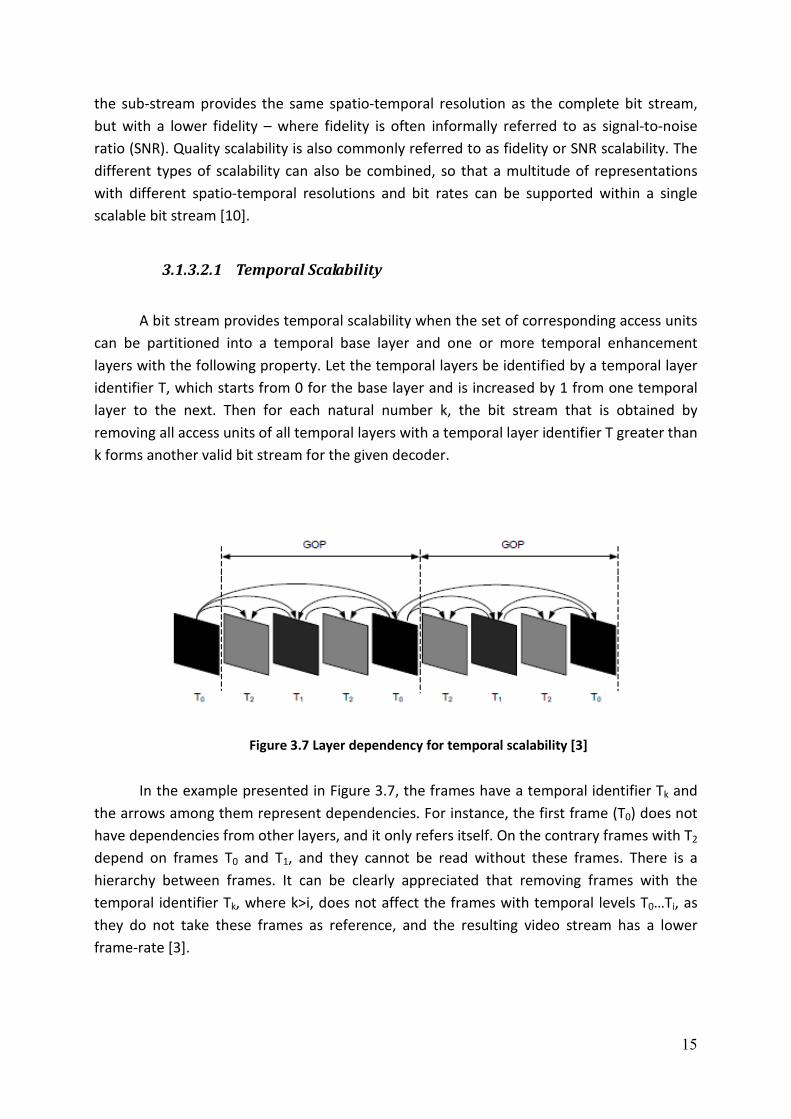
Figure 3.7 Layer dependency for temporal scalability [3]
In the example presented in Figure 3.7, the frames have a temporal identifier Tk and
the arrows among them represent dependencies. For instance, the first frame (T0) does not
have dependencies from other layers, and it only refers itself. On the contrary frames with T2
depend on frames T0 and T1, and they cannot be read without these frames. There is a
hierarchy between frames. It can be clearly appreciated that removing frames with the
temporal identifier Tk, where k>i, does not affect the frames with temporal levels T0…Ti, as
they do not take these frames as reference, and the resulting video stream has a lower
frame-rate [3].

16
3.1.3.2.2 Spatial Scalability
When spatial scalability is applied, the video is encoded at multiple spatial resolutions
(picture size). The data and decoded samples of lower resolutions can be used to predict
data or samples of higher resolutions in order to reduce the bit rate to encode the higher
resolutions.
Each layer corresponds to a supported spatial resolution and is referred to by a
spatial layer or dependency identifier D. The dependency identifier for the base layer is
equal to 0, and it is increased by 1 from one enhancement spatial layer to the next. As for
single layer-coding, motion-compensated prediction and intra-prediction are employed in
each layer. But in order to improve coding efficiency in comparison to simulcasting, different
spatial resolutions, additional so-called inter-layer prediction mechanisms are incorporated.
Figure 3.8 Layer dependency for spatial scalability [9]
In Figure 3.8 an example of what explained above can be seen. The frames below
represent the base layer while the frames above depict the enhancement layer. In this case,
there are not only dependencies among frames, but also a hierarchical connection between
the two layers is present when spatial resolution applied. As a first step, the base layer is
decoded providing a base quality spatial resolution. Afterwards, if enhancement layer is
received successfully, the decoding of the enhancement layer will provide an increase in the
overall decoded video resolution and so on with the different enhancement layers received
[3].

17
3.1.3.2.3 Quality Scalability
Quality scalability can be considered as a special case of spatial scalability with
identical picture sizes for base and enhancement layer. This case, which is also referred to as
coarse-grain quality scalable coding (CGS), is supported by the general concept for spatial
scalable coding as described above. The same inter-layer prediction mechanisms are
employed, but without using the corresponding upsampling operations. When utilizing inter-
layer prediction, a refinement of texture information is typically achieved by re-quantizing
the residual texture signal in the enhancement layer. A smaller quantization step size
relative to that used for the preceding CGS layer is used for the higher layer. As a specific
feature of this configuration, the deblocking of the reference layer intra signal for inter-layer
intra prediction is omitted. Furthermore, inter-layer intra and residual prediction are directly
performed in the transform coefficient domain in order to reduce the decoding complexity.
The CGS concept only allows a few selected bit rates to be supported in a scalable bit
stream. In general, the number of supported rate points is identical to the number of layers.
Switching between different CGS layers can only be done at defined points in the bit stream.
Furthermore, the CGS concept becomes less efficient, when the relative rate difference
between successive CGS layers gets smaller. Especially for increasing the flexibility of bit
stream adaptation and error robustness, but also for improving the coding efficiency for bit
streams that have to provide a variety of bit rates, a variation of the CGS approach, which is
also referred to as medium-grain quality scalability (MGS), is included in the SVC design. The
differences to the CGS concept are a modified high-level signaling, which allows a switching
between different MGS layers in any access unit, and the so-called key picture concept,
which allows the adjustment of a suitable trade-off between drift and enhancement layer
coding efficiency for hierarchical prediction structures. The dependency between layers
would be similar to the one in Figure 3.8 but without a difference in resolution between
pictures [9].
3.1.3.2.4 Combined Scalability
Although the three types of scalability have been described separately, any
combination of them could be applied to obtain a new scalability profile of the encoded
video. In Figure 3.9, an encoder structure with two spatial layers and combined scalability is
depicted.

18
Figure 3.9 Example of a SVC encoder with different scalabilities
While in this example the dependency layers represent different spatial resolutions,
they could have had identical spatial resolution, where simple coarse-grain-scalability (CGS)
would be applied. In this figure, each of the dependency layers has two quality refinement
layers. When there is more than one quality representation, it becomes necessary to signal
which of these is employed for inter-layer prediction of higher dependency layers. For
quality refinement, the preceding quality layer is always employed for inter-layer prediction.
3.2 Video Transmission
3.2.1 Introduction
Advance and Scalable Video Coding are used nowadays in a wide range of
applications ranging from multimedia messaging, video telephony and video conferencing
over mobile TV, media storage (high definition DVD…), wireless and Internet video
streaming, to standard and high-definition TV broadcasting. In the regard of this work,
H.264/AVC and SVC are used to encode video with the aim of transmitting it over a
transmission channel [3].
The transmission channel refers to the element used to convey data from a sender to
a receiver. Due to transmission channels are physically not perfect, these channels suffer
from noise, distortion, interference, fading, etc… which lead into transmission errors or
losses. In all the mentioned cases, if data is transmitted, e.g., an encoded video stream,
there is some probability that the received message will not be identical to the transmitted
data or even worst, it will get lost.

19
This work will focus on transmission channels based on the Internet network model
when transmitting user datagram protocol packets. That is, an open network in which UDP
protocol over the Internet Protocol is used to transmit the packetized data, in this study, the
encoded video packets.
Figure 3.10 OSI model with matching internet model and some exemplary protocols
3.2.2 Internet Protocol (IP)
The Internet Protocol (IP) is the principal communications protocol used for relaying
datagrams (packets) across an internetwork using the Internet Protocol Suite (set of network
protocols used for the Internet). IP is responsible for routing packets across network
boundaries and is the primary protocol that establishes the Internet.
IP has the task of delivering datagrams from the source host to the destination host
solely based on their addresses. IP is a connectionless protocol and does not need circuit
setup prior to transmission. For this purpose, IP defines addressing methods and structures
for datagram encapsulation. As consequence of its design, the Internet Protocol only
provides best effort delivery and its service can also be characterized as unreliable. In
network architectural language it is a connection-less protocol, in contrast to so-called
connection-oriented modes of transmission. The lack of reliability allows any of the following
fault events to occur:
� data corruption
� lost data packets
� duplicate arrival

20
� out-of-order packet delivery
The most widely used version of IP today is Internet Protocol Version 4 (IPv4).
However, IP Version 6 (IPv6) is also beginning to be supported. IPv6 offers better addressing
capacities, security, full compatibility with IPv4 and other features to support large
worldwide networks.
The only assistance that the Internet Protocol provides in Version 4 (IPv4) is to ensure
that the IP packet header is error-free through computation of a checksum at the routing
nodes. This has the side-effect of discarding packets with bad headers on the spot. In this
case no notification is required to be sent to either end node, although a facility exists in the
Internet Control Message Protocol (ICMP) to do so [11].
3.2.3 User Datagram Protocol (UDP)
The User Datagram Protocol (UDP) is one of the core members of the Internet
Protocol Suite. With UDP, computer applications can send messages, in this case referred to
as datagrams, to other hosts on an Internet Protocol (IP) network without requiring prior
communications to set up special transmission channels or data paths.
UDP uses a simple transmission model without implicit hand-shaking dialogues for
providing reliability, ordering, or data integrity. Thus, UDP provides an unreliable service and
datagrams may arrive out of order, appear duplicated, or go missing without notice. UDP
assumes that error checking and correction is either not necessary or performed in the
application, avoiding the overhead of such processing at the network interface level. Time-
sensitive applications often use UDP because dropping packets is preferable to waiting for
delayed packets, which may not be an option in a real-time system [12].
Figure 3.11 Pseudo Header used for the IP checksum calculation

21
The present work focuses on low and high delay video applications such as Video
Conferencing, Real Time Video Broadcasting, Mobile TV,etc. In this regard, UDP is the
protocol that will be used to perform all the simulations, because as explained before, is the
commonly used protocol for time sensitive applications.
3.3 Error Detection and Correction
3.3.1 Introduction
Data transmission over wired or wireless channels is typically subject to transmission
errors caused by multiple effects such as congestion or interferences. In particular, video
data is very sensitive to transmission errors. Due to inter-frame predictions, single errors
may cause heavy error propagation to predicting frames. This becomes more critical, when
layered video coding such as scalable video coding (SVC) is applied. Due to additional inter-
layer prediction, the amount of dependencies increases highly across the layers.
Error detection techniques allow detecting such errors, while error correction enables
the detection and additionally the reconstruction of the original data. Therefore, error
detection and correction are techniques that enable reliable delivery of digital data over
unreliable communication channel.
Error control techniques such as Automatic Repeat reQuest (ARQ) or Forward Error
Correction are used to cope with a several amount of the aforementioned errors. By ARQ,
reliable data transmission can be achieved over an unreliable channel by means of
acknowledgements, messages sent by the receiver indicating correct reception, and
timeouts, specified time periods allowed to elapse before an acknowledgement is to be
received. If the sender does not receive an acknowledgement from the receiver before the
timeout elapses, usually a re-transmission of one or several packets is needed. On the other
hand, FEC techniques provide also a reliable transmission over a non error-free channel, but
skipping any kind of re-transmission and thus, reducing drastically the delay at reception.
Using FEC, the sender adds redundant data to its packets which allow the receiver to detect
and correct errors without the need to ask the sender for additional transmissions.
Standard FEC schemes applied to layered media such as SVC generate redundant data
independently for each layer. Hence, taking into account the source information of each
Layer, different redundant FEC packet-blocks will be generated for each layer separately. I.e.
if redundant and source data from different layers is received, the FEC data protection
become useless since there is no information of the received source data contained on it. As
a different forward error correction technique applied to layered media, LA-FEC generates

22
the parity information across layers within the media stream in such a way, that the
protection of some layers can be used additionally for the correction of some other different
layers. Generally, in layered video transmission some layers are more important than others.
Therefore, LA-FEC provides additional protection for the most important layers using
redundancy from those of less importance.
3.3.2 Automatic Repeat Request
Automatic Repeat reQuest (ARQ) is an error control method for data transmission
that makes use of error-detection codes, acknowledgment and/or negative acknowledgment
messages, and timeouts to achieve reliable data transmission.
Usually, when the transmitter does not receive the acknowledgment before the
timeout occurs, it retransmits the frame until it is either correctly received or the error
persists beyond a predetermined number of retransmissions.
Figure 3.12 ARQ protocol
ARQ is appropriate if the communication channel has varying or unknown capacity,
such as is the case on the Internet. However, ARQ requires the availability of a back channel,
results in possibly increased latency due to retransmissions, and requires the maintenance of
buffers and timers for retransmissions, which in the case of network congestion can put a
strain on the server and overall network capacity [13].
Three types of ARQ protocols are Stop-and-wait ARQ, Go-Back-N ARQ, and Selective
Repeat ARQ.

23
3.3.3 Forward Error Correction
In a communication system that employs forward error-correction coding, a digital
information source sends a data sequence comprising k bits of data to an encoder. The
encoder inserts redundant (or parity) bits, thereby outputting a longer sequence of n code
bits called a codeword. On the receiving end, codewords are used by a suitable decoder to
extract the original data sequence.
Codes are designated with the notation (n, k) according to the number of n output
code bits and k input data bits. The ratio k/n is called the rate, R, of the code and is a
measure of the fraction of information contained in each code bit. For example, each code
bit produced by a (6, 3) encoder contains 1/2 bit of information.
n
kR = (3.1)
Another metric often used to characterize code bits is redundancy, expressed as (n–
k)/n. Codes introducing large redundancy (that is, large n–k or small k/n) convey relatively
little information per code bit. Codes that introduce less redundancy have higher code rates
(up to a maximum of 1) and convey more information per code bit. Large redundancy is
advantageous because it reduces the likelihood that all of the original data will be wiped out
during a single transmission.
The advantages of forward error correction are that a back-channel is not required
and retransmission of data can often be avoided (at the cost of higher bandwidth
requirements, on average). FEC is therefore applied in situations where retransmissions are
relatively costly or impossible [14].
The two main categories of FEC codes are linear block codes and convolutional codes.
The present work is based on linear block codes in which FEC redundancy is generated to
cope with the transmission looses.
24
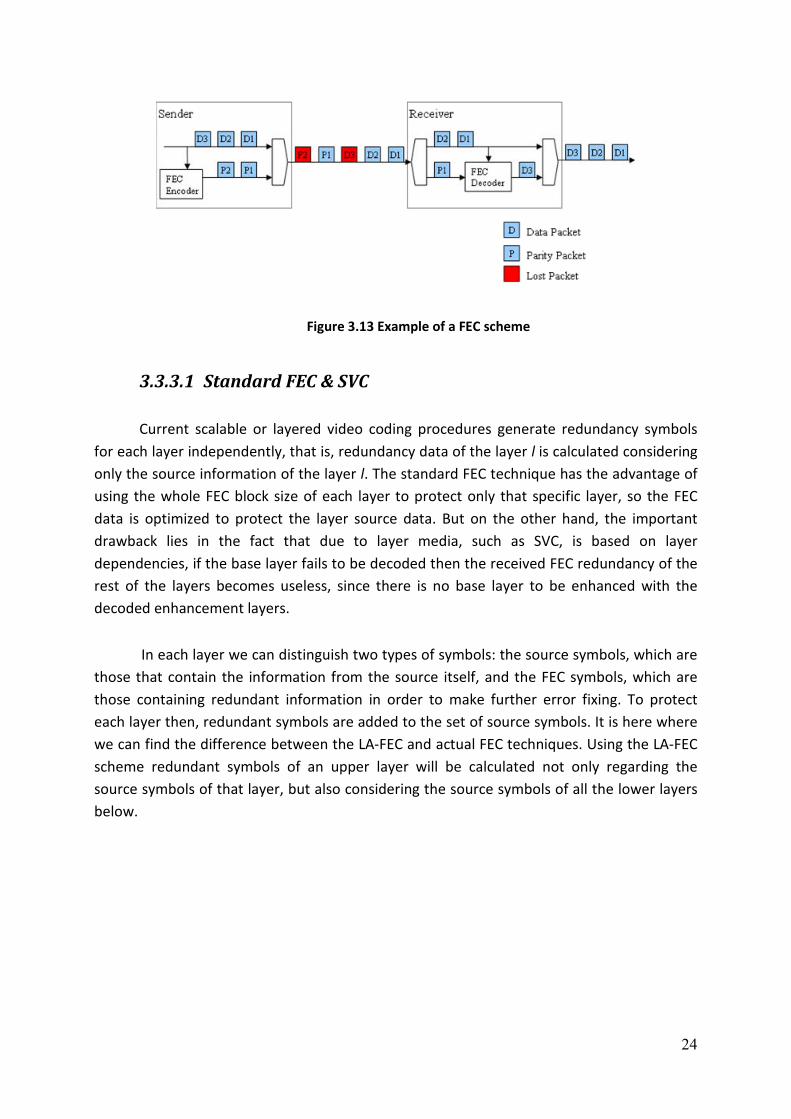
Figure 3.13 Example of a FEC scheme
3.3.3.1 Standard FEC & SVC
Current scalable or layered video coding procedures generate redundancy symbols
for each layer independently, that is, redundancy data of the layer l is calculated considering
only the source information of the layer l. The standard FEC technique has the advantage of
using the whole FEC block size of each layer to protect only that specific layer, so the FEC
data is optimized to protect the layer source data. But on the other hand, the important
drawback lies in the fact that due to layer media, such as SVC, is based on layer
dependencies, if the base layer fails to be decoded then the received FEC redundancy of the
rest of the layers becomes useless, since there is no base layer to be enhanced with the
decoded enhancement layers.
In each layer we can distinguish two types of symbols: the source symbols, which are
those that contain the information from the source itself, and the FEC symbols, which are
those containing redundant information in order to make further error fixing. To protect
each layer then, redundant symbols are added to the set of source symbols. It is here where
we can find the difference between the LA-FEC and actual FEC techniques. Using the LA-FEC
scheme redundant symbols of an upper layer will be calculated not only regarding the
source symbols of that layer, but also considering the source symbols of all the lower layers
below.

25
Figure 3.14 Generation of redundancy for each layer by means of standard FEC schemes
In Figure 3.14 is depicted a schematic representation of how the FEC data is
calculated when using standard layered FEC protection schemes.
As it has already explained, in layered media information data is divided in layers.
Each layer consists of two main data blocks: the original source data and the redundancy
data generated to protect the source data, the so-called FEC source block (see Figure 3.15).
Different layers can be protected with different code rates depending on the protection
required.
For instance, when encoding the base layer of a video stream which size is 164 Kbps
using a code rate of 1/3, the overall size S of the base layer plus the FEC protection results
in:
5463.0
164KbpsS == (3.2)
Therefore, the redundancy R added to protect the base layer is:
KbpsKbpsKbps
R 3821643.0
164=−= (3.3)
As can easily be beheld in the explained example, a lower code rate chosen leads into
a higher protection given to the source data.
Moreover, the size of the FEC redundancy data is called FEC source block length.
Before generating redundancy data, a FEC algorithm needs to wait an amount of time t until
a certain amount of source data is collected in what was defined as the FEC source block.

26
Therefore, a receiver has to wait a time t until it can use the FEC data. In Figure 3.15 is
shown a graphical display of how a scalable layer is divided in source and FEC data.
Figure 3.15 Scalable layer divided into Source and FEC data
3.3.3.2 Layer Aware FEC & SVC
Layer-Aware FEC (LA-FEC) [15] is a novel scheme for layered media such as SVC or
MVC (Multiple Video Coding). LA-FEC generates the parity information across layers within
the media stream in such a way, that the protection of less important layers can be used for
the correction of more important layers.
As explained in Section 3.3.3.1, in traditional FEC schemes for layered media
transmission the redundancy is separately generated for each scalable layer. However, if the
base layer cannot be corrected due to transmission errors, most of the enhancement layer
information cannot be used due to missing reference pictures. The main idea of LA-FEC
schemes, i.e. LA-FEC applied to SVC, is to generate the parity data of the enhancement
layers following existing dependencies within the video stream.
Figure 3.16 Generation of redundancy over layers following existing dependencies within
the media stream
Using LA-FEC, redundancy symbols of the less important SVC enhancement layers can
jointly be used with symbols of more important layers (e.g., base layer) for error correction
as shown in Figure 3.16. This effect comes without any increase in bit rate, and improves the
reliability of the whole service. Figure 3.17 depicts a simplified example with base and one
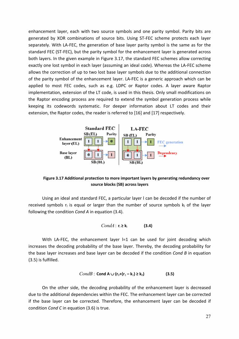
27
enhancement layer, each with two source symbols and one parity symbol. Parity bits are
generated by XOR combinations of source bits. Using ST-FEC scheme protects each layer
separately. With LA-FEC, the generation of base layer parity symbol is the same as for the
standard FEC (ST-FEC), but the parity symbol for the enhancement layer is generated across
both layers. In the given example in Figure 3.17, the standard FEC schemes allow correcting
exactly one lost symbol in each layer (assuming an ideal code). Whereas the LA-FEC scheme
allows the correction of up to two lost base layer symbols due to the additional connection
of the parity symbol of the enhancement layer. LA-FEC is a generic approach which can be
applied to most FEC codes, such as e.g. LDPC or Raptor codes. A layer aware Raptor
implementation, extension of the LT code, is used in this thesis. Only small modifications on
the Raptor encoding process are required to extend the symbol generation process while
keeping its codewords systematic. For deeper information about LT codes and their
extension, the Raptor codes, the reader is referred to [16] and [17] respectively.
Figure 3.17 Additional protection to more important layers by generating redundancy over
source blocks (SB) across layers
Using an ideal and standard FEC, a particular layer l can be decoded if the number of
received symbols rl is equal or larger than the number of source symbols kl of the layer
following the condition Cond A in equation (3.4).
:CondA rl ≥ kl (3.4)
With LA-FEC, the enhancement layer l=1 can be used for joint decoding which
increases the decoding probability of the base layer. Thereby, the decoding probability for
the base layer increases and base layer can be decoded if the condition Cond B in equation
(3.5) is fulfilled.
:CondB Cond A ∪∪∪∪ (r0+(r1 – k1) ≥ k0) (3.5)
On the other side, the decoding probability of the enhancement layer is decreased
due to the additional dependencies within the FEC. The enhancement layer can be corrected
if the base layer can be corrected. Therefore, the enhancement layer can be decoded if
condition Cond C in equation (3.6) is true.

28
:CondC Cond B ∩∩∩∩ (r1 ≥ k1) (3.6)
However, due to the enhancement layer data is useless in case of lost base layer,
there is no significant impact on the perceived video quality when applying LA-FEC.

29
4. LLAAYYEERREEDD VVIIDDEEOO
TTRRAANNSSMMIISSSSIIOONN CCHHAALLLLEENNGGEESS This work has the target of analyzing the gain brought by the Layer-Aware FEC new
approach compared to a Standard FEC technique over a channel with variable throughput.
Two main scenarios have been studied: firstly a one-hop connection is simulated between
two users, afterwards, in second term, a more complex scenario based on a star
configuration model is performed, in which the different users exchange information
through a central node which organizes and coordinates the communication.
4.1 Simulator Chain
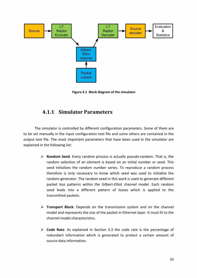
The study of the previously mentioned scenarios has been carried out by means of a
network simulator. The simulator reproduces a one-hop transmission between two users
over a fixed model channel. In Figure 4.1 is depicted a block diagram of the used simulator.
The simulator starts by loading and fragmenting the video file, which want to be sent over,
into the Source block on the first part of the simulator. Afterwards, depending on the
configuration parameters, a LT Raptor encoder [16] [17] is used to encode and generate the
proper FEC/LA-FEC redundancy protection for each layer. Transmission losses are applied to
the transmitted packets while simulating the sending in the Gilbert-Elliot channel block.
Later, packets are collected by the LT Raptor decoder at reception and then, a Forward Error
Correction (FEC/LA-FEC) decoding process is carried out. Depending on the lost packets and
on the recovered source data the simulator is able to generate the proper statistics for the
transmission which are stored in an output text file.
30
Source
LT
Raptor
Encoder
Gilbert-
Elliot
channel
Packet
Losses
LT
Raptor
Decoder
Source
decoder
Evaluation
&
Statistics
Figure 4.1 Block diagram of the simulator.
4.1.1 Simulator Parameters
The simulator is controlled by different configuration parameters. Some of them are
to be set manually in the input configuration text file and some others are contained in the
output text file. The most important parameters that have been used in the simulator are
explained in the following list:
� Random Seed: Every random process is actually pseudo-random. That is, the
random selection of an element is based on an initial number or seed. This
seed initializes the random number series. To reproduce a random process
therefore is only necessary to know which seed was used to initialize the
random generator. The random seed in this work is used to generate different
packet loss patterns within the Gilbert-Elliot channel model. Each random
seed leads into a different pattern of losses which is applied to the
transmitted packets.
� Transport Block: Depends on the transmission system and on the channel
model and represents the size of the packet in Ethernet layer. It must fit to the
channel model characteristics.
� Code Rate: As explained in Section 3.3 the code rate is the percentage of
redundant information which is generated to protect a certain amount of
source data information.

31
� Packet Losses: The encoded source data is distributed in packets containing
data. Those packets are sent over a transmission channel. In the simulator, the
channel reproduces losses which result into lost packets at the reception.
� PSNR: Stands for peak signal-to-noise ratio. Is a term for the ratio between the
maximum possible power of a signal and the power of corrupting noise that
affects the fidelity of its representation.
� Frame: As depicted in Figure 3.1, is one of the many still images which
compose the complete moving picture or video stream.
� Freeze Frame: In video transmission, when a frame is lost due to losses in the
channel or whichever other reason, the lost frame may be replaced with the
previous decoded frame instead. The duplicated frame is called a freeze
frame.
� Bit Rate: Is the number of bits that are conveyed or processed per unit of
time. In other words, it measures how much data is transmitted in a given
amount of time. Bit rate can also describe the quality of an audio or video file.
For example, an MP3 audio file that is compressed at 192 Kbps will have a
greater dynamic range and may sound slightly more clear than the same audio
file compressed at 128 Kbps. This is because more bits are used to represent
the audio data for each second of playback. The same effect happens with
video coding.
In Figure 4.2 can be seen a screenshot of the configuration parameters in the
simulator main configuration screen. In the example shown in Figure 4.2, a code rate of 0.68
is used to protect the base layer while a code rate of 0.76 is used for the enhancement layer.
Can be seen as well the Gilber-Elliot channel parameters which will be used to carry out the
packet losses in the channel using the random seed 1 (more details of the channel
reproduction will be explained in detail in Section 4.1.2).

32
Figure 4.2 System simulator. Input parameter screen
4.1.2 Simulator Channel
To simulate packet loss due to congestion the simulator assumed the loss rates
probabilities described in [18] and a channel reproduction based on the Gilbert Elliot model.
Introducing the loss probabilities analyzed in [18] into the Gilbert Elliot Model we obtain the
characteristics of the channel losses, which are an IP packet error rate of 22 % with a mean
burst length error average of 1.8 IP packets.
In the performed simulations was modified the traditional encapsulation scheme in
order to generate the IP packets equal size to the Maximum Transmission Unit size (MTU), as
will be explained in Section 4.1.3, which for the performed simulations means a size of 1400
bytes. Occasionally some IP packets result with a smaller size due to fragmentation issues.
The above mentioned modification has been done in order to make equal the probability of
losing one IP packet with the probability of losing one MTU. Previously, more than one IP
packet could be contained in one MTU, therefore, losing an entire MTU could occur when
just one of the IP packets contained on it gets lost.

33
Figure 4.3 State diagram of the Gilbert Elliot model used for packet loss simulation
The Gilbert Elliot diagram is based on a two state Markov-model as shown in Figure
4.3. State 0 represents the state of successful arrival of the packet, while state 1 represents
the state of packet lost. The transition probability p10 from state 1 to state 0, the transition
probability p01 from state 0 to state 1 as well as the IP packet error rate and the average
burst length are summarized in Table 4.1. For deep detailed calculations of the mentioned
data resort to [18].
State Transition Channel Parameters
p10 p01 IP packet error
rate
Average burst
length
0.5479 0.0986 22% 1.8 IP packets
Table 4.1 Parameters of Gilbert Elliot Channel Model [18]
4.1.3 Simulator Software
In order to analyze the behavior of the two FEC protection schemes, a simulator
already developed in C++ by the Multimedia Communications Group of Fraunhofer Heinrich-
Hertz-Institute has been adapted to our needs. Some of the important changes that have
been done in the simulator are:
� The two scalable levels (or layers) are fragmented in several fragmented packets
as can be seen in Figure 4.4. An adaptation to the main simulator has been
performed in order to encapsulate every fragmented packet from the two
scalable levels in exactly one IP packet. It has been done in this way due to the
channel model that has been used in this work. This channel is based on the
Gilbert Elliot model analyzed in [18] and therefore the loss probability on this
channel model is applied to each IP packet. That’s why the mentioned adaptation
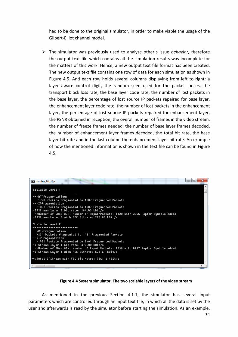
34
had to be done to the original simulator, in order to make viable the usage of the
Gilbert-Elliot channel model.
� The simulator was previously used to analyze other´s issue behavior; therefore
the output text file which contains all the simulation results was incomplete for
the matters of this work. Hence, a new output text file format has been created.
The new output text file contains one row of data for each simulation as shown in
Figure 4.5. And each row holds several columns displaying from left to right: a
layer aware control digit, the random seed used for the packet looses, the
transport block loss rate, the base layer code rate, the number of lost packets in
the base layer, the percentage of lost source IP packets repaired for base layer,
the enhancement layer code rate, the number of lost packets in the enhancement
layer, the percentage of lost source IP packets repaired for enhancement layer,
the PSNR obtained in reception, the overall number of frames in the video stream,
the number of freeze frames needed, the number of base layer frames decoded,
the number of enhancement layer frames decoded, the total bit rate, the base
layer bit rate and in the last column the enhancement layer bit rate. An example
of how the mentioned information is shown in the text file can be found in Figure
4.5.
Figure 4.4 System simulator. The two scalable layers of the video stream
As mentioned in the previous Section 4.1.1, the simulator has several input
parameters which are controlled through an input text file, in which all the data is set by the
user and afterwards is read by the simulator before starting the simulation. As an example,

35
in the input text file can be changed parameters such as the FEC source block length, the
code rates applied to each layer, the channel type, the channel loose probabilities, the
transport block size, etc.
This work entails thousands of simulations. Huge data output simulation files are
needed to test and compare the Layer-Aware and the Standard-FEC scheme. Different FEC
source block lengths, different code rates applied to each layer, different overall bit rate of
the protected stream, etc. have to be tested and afterwards analyzed. To achieve statistically
correct results, every single simulation has to be done using a high number of different
random seeds to reproduce the packet losses within the Gilbert-Elliot channel, to consider in
the end an average of all of them when analyzing results.
Figure 4.5 Detail of an exemplary StatOut file of the simulator. In example the code rates
applied are 0.86 for base layer and 0.66 for enhancement layer. The random seed, which initiates
the Gilbert-Elliot model, is changed in each simulation

36
Carry out all the simulations manually would take an enormous amount of time. To
automate repetitive simulations several PERL [26] language programmed scripts which are
meant to automatically change the input text file of the simulator with the different chosen
values we want to simulate in a loop have been used. This allows looping through different
settings with new input data without the need of changing anything by hand. For the
succeeding analysis of the data, the simulation results stored within the StatOut text files (cf.
Figure 4.5) are used.
Figure 4.6 Statistics after transmission, reception and correction for a LA-FEC simulation.
In the next step, the StatOut text files, such as the one shown in Figure 4.5, are
processed in order to analyze performance. To perform all the data processing and value the
calculations it was decided to use Matlab [27]. Different Matlab functions have been
programmed to carry out different functionalities with the StatOut data files such as e.g.
PSNR average calculations, locate simulations with certain output bit rate, minimization and
maximization of different result parameters. Further more complex scripts were required to
execute bit rate optimizations based on maximum PSNR or minimum IP packet loses
(explained in Section 4.4 and Section 4.5), simulation of the second star-model scenario
(explained in Section 6), extraction of base layer symbols from a full raptor symbol
(explained in Section 6.2.1.1), etc.
4.1.4 Simulator Video Stream
In all the performed simulations in this work the same scalable video coding stream
has been used. To reduce the overall system delay, a low delay SVC bit stream with two
layers, base (qCIF) and enhancement (CIF), at a frame rate of 30 Hz has been encoded [3].
The sequence, of about 30 seconds, is a concatenation of the ITU-T test sequences

37
Carphone, Foreman and Mother&Daughter using low delay SVC coding (Scalable Baseline
Profile, JSVM9.17).
During the transmission, and as was explained in Section 4.1.2, some of the frames
that compose the video stream may get lost due to the simulated transmission errors. In
case of frame losses, freeze frame error concealment is used, where the last decoded picture
is just copied. In case only the enhancement layer gets lost, the up scaled qCIF layer was
used for PSNR calculation. A summary of the encoding parameters for SVC can be found in
Table 4.2.
Quality Video Rate [kbps] Avg. PS"R [dB]
SVC – Base layer qCIF@30Hz 164 31.87 (upscaled)
SVC – Base +
Enhancement layer CIF@30Hz 544 38.64
Table 4.2 SVC media stream characteristics
4.2 Influence of the FEC source block length
As explained in Section 3.3.3.1, the FEC source block length refers to the period of
time of data within a source block, from which the FEC data is calculated. The redundant
data is in fact based on the source data; therefore, a FEC algorithm which generates parity
data has to wait an amount of time t until a certain quantity of source data is collected (In
Figure 4.7 the time between t0 and t1). In the same way, a receiver needs to wait a time t
until it can use the FEC data.

38
Figure 4.7 FEC source block extracted from the media stream to be sent to the FEC
generator
The selection of the FEC source block length is a decisive issue when targeting
different video applications. The FEC source block length is directly related to the overall
delay of the system. When a higher FEC source block length is chosen the latency of the
system increases due to receiver client has to wait until all the packets of the specific source
block have been received, on the contrary, if the FEC source block length is low, the general
latency of the system decreases. For instance, if a coding process is performed with the aim
of providing a video-conference system, the FEC source block length has to be kept small
(around 150ms according to the ITU recommendation G.114 [19]) in order to avoid long
waits or voice interruptions among the participants of the conversation. On the other hand,
for instance the provided service is based on mobile TV, a higher delay up to two seconds is
permitted, so a larger FEC block can be chosen. An example is depicted in Figure 4.8.

39
0 2 4 6 8 10 12 14 16 1826
28
30
32
34
36
38
40
FEC Source Block Length [seconds]
PSNR Average [dB]
ST-FEC / EEP
ST-FEC / UEP
LA-FEC / EEP
LA-FEC / UEP
Figure 4.8 Video applications require different FEC source block length and therefore
different delay
Moreover, when using a bursty channel, the size of the FEC block influences
significantly on the quality of the received information at reception. Depending on the
chosen FEC source block length the receiver has to carry out the decoding process based on
different waiting times and this fact makes the overall system performance behave not
always in the same way in terms of PSNR quality.
Simulations have been performed to show how the achieved PSNR quality changes
when employing different FEC source block lengths at the same code rate for each data
source block. Due to the longer source block, the overall output bit rate in this case is
different for every FEC length simulation point.
Afterwards, a more reliable comparison has been carried out and simulations were
performed fixing the bit rate in all of the FEC source block length simulation points. In this
regard, it was chosen the proper code rate for the base and the enhancement layer and for
each FEC length simulation in order to output several bit rates of 700 Kbps, 800 Kbps, 900
Kbps and 1Mbps. Also, two different protection schemes have been investigated. First,
protecting both layers with the same code rate, which is usually called an Equal Error
Protection scheme (EEP). And next, another protection technique which is known as
Unequal Error Protection (UEP) was tried. In this second case, each layer is protected in a
different way, then, different code rates for each layer are selected depending on the
desired behavior and the characteristics of the system. For our simulations, the chosen code
rates have been the ones which lead in a higher PSNR in reception.

40
0 2 4 6 8 10 12 14 16 1829
31
33
FEC Source Block Length [seconds]
Average PSNR [dB]
250 Seeds
ST-FEC
LA-FEC
Figure 4.9 Average PSNR vs FEC source block length for ST-FEC and LA-FEC protection
schemes. Both layers equal protected with a FIXED code rate of 0.7
Figure 4.9 shows the performance of ST-FEC and LA-FEC techniques for different
source block lengths when applying an equal error protection scheme with a code rate of 0.7
for both layers. At low FEC block sizes the difference between the ST-FEC and LA-FEC is more
noticeable achieving almost 1 dB at some points. The two curves start to merge at higher
FEC block lengths converging at the same point at around a FEC length of 17 seconds.
For the second simulations set, the code rates of the two layers were fixed for each
FEC source block length in order to obtain a constant bit rate for all the simulated FEC length
points. The behavior of the ST-FEC and the LA-FEC technique for four constant bit rates, 700,
800, 900, and 1000 Kbps was analyzed.
In Figure 4.10 a), when the output bit rate is equal to 700 Kbps, it can be seen that
there is not enough throughput available to see a useful comparison between the two
schemes. Furthermore, an UEP (Unequal Error Protected) scheme always performs better
than the EEP (Equal Error Protected).

41
0 5 10 15 2024
26
28
30
32
34
FEC Source Block Length [sec]
PSNR [dB]
a) BitRate 700 Kb/s
ST-FEC / EEP
ST-FEC / UEP
LA-FEC / EEP
LA-FEC / UEP
0 5 10 15 2026
28
30
32
34
36
38
40
FEC Source Block Length [sec]
PSNR [dB]
b) BitRate 800 Kb/s
0 5 10 15 2026
28
30
32
34
36
38
40
FEC Source Block Length [sec]
PSNR [dB]
c) BitRate 900 Kb/s
0 5 10 15 2028
30
32
34
36
38
40
FEC Source Block Length [sec]
PSNR [dB]
d) BitRate 1 Mb/s
Figure 4.10 Average PSNR vs FEC source block length for ST-FEC and LA-FEC protection
schemes as well as for equal (EEP) and unequal (UEP) error protection in the layers. Code Rates for
the two layers chosen in order to output a total bit rate of a) 700 Kbps, b) 800 Kbps, c) 900 Kbps
and d) 1 Mbps.
When the simulated bit rate goes up to 800 Kbps (Figure 4.10 b)) there is the biggest
difference among the ST-FEC and the LA-FEC schemes. For the LA-FEC, when UEP or EEP
protected, it behaves almost the same, which doesn't happen for ST-FEC, where the
difference is noticeable when applying EEP or UEP. For the simulated bit rates of 900 Kbps
and 1 Mbps the difference among the several FEC protection schemes keeps going lower as
shown in Figure 4.10 c) and Figure 4.10 d).
Analyzing the described figures can be concluded that depending on the bit rate of
the video stream there is a bit rate area in which the difference, when applying ST-FEC and
LA-FEC, is maximum. In the previous explained simulations, that bit rate area is surrounding
800 Kbps. This bit rate area is directly related to the overall video stream bit rate. In this
work, the video stream consists of 544 Kbps; so at protections of around 250 Kbps of

42
redundancy, resulting a total of around 800 Kbps, is where the LA-FEC scheme sets the
highest gain compared to the ST-FEC.
Moreover, there is also a dependency between the FEC source block length and the
PSNR at reception in the different schemes. A smaller FEC source block length produces a
higher difference in PSNR at reception because when the FEC source block length is high, the
decoder has always a lot of FEC information of the source block, and then, it is always
possible to decode properly. On the other hand, when the FEC source block is small and
then, there is not so much FEC information protecting each data source block, is when the
LA-FEC scheme outperforms clearly the ST-FEC schemes.
4.3 Influence of the Code Rate
The code rate of a forward error correction (FEC) code can be understood as what
portion of the total amount of data (source plus redundancy) is useful or non-redundant. As
explained in Section 3.3.3, the code rate is typically a fractional number. If the code rate is
k/n bits of useful information, the coder generates totally n bits of data, of which n-k are
redundant. So in case of no redundant information is added, the code rate results to be
equal to 1 (k/k = 1). That is, the lower the code rate is, the higher the protection
(redundancy) is applied, and vice versa, when the code rate is high (close to 1) less
redundancy is generated. Note that when working with large amount of information bit
streams the code rate is often given as a decimal number between 0 and 1 instead of
keeping the fractional way.
0.55 0.6 0.65 0.7 0.75 0.8 0.85 0.9 0.95 125
30
35
40
Code Rate
Average PSNR [dB]
LA-FEC
FEC SB length= 0.132 ms
FEC SB length= 0.264 ms
FEC SB length= 0.528 ms
Figure 4.11 Average PSNR vs Code Rate for different lengths of FEC source block. Both
layers equal error protected and LA-FEC applied.

43
In Figure 4.11 is depicted the average PSNR obtained at reception for a one single
connection scenario when the code rate is increased from 0.55 to 1. Both layers have been
equal error protected in this simulation. The average PSNR obtained for each code rate has
been calculated from several different simulations over the Gilbert-Elliot model with
different random seeds. Moreover, different FEC source block lengths have been simulated
going from 0.132ms, which for our 30fps video stream means a length equal to 4 frames, to
0.528ms, or 16 frames duration. The influence of the code rate can be clearly seen in the
Figure 4.11, the lower the code rate is (more redundancy), the higher PSNR is achieved at
reception. The influence of the FEC source block length is noticeable again in this simulation.
As can be seen in the Figure 4.11, when a larger FEC length is used, the PSNR quality
obtained in reception is higher. This effect is more obvious when the code rate decreases,
taking a look can be seen how around code rates of 0.6 the difference between a FEC source
block length of 4 and 16 frames is almost 3 dB, whereas when the code rate is close to 1 the
three analyzed FEC lengths behave almost in the same way in terms of PSNR quality
achieved in reception.
4.4 Code Rate Optimization by Maximum PSNR
In this section will be introduced the variable throughput channel conditions and how
the Layer Aware FEC performs across different channel capacities.
It's already clear now how the code rate influences the encoder´s output bit rate of
the video stream: when the code rate applied to each layer is equal to 1 the encoder's
service bit rate results to be the same as the original data stream, i.e. no protection is
applied. Therefore, when the code rate is reduced, a higher protection is generated which
leads to a larger amount of redundant data and hence, a higher output service bit rate.
As a first step to understand how the two schemes, ST-FEC and LA-FEC, perform over
variable throughput, a one-hop scenario has been simulated with the following
characteristics and constraints:
• Throughput going from 800 Kbps to 2.6 Mbps with variable Kbps step for the
different areas.
• Code rate protection for the base and the enhancement layer going from 1 to 0.2
• 50 different random seeds used in the Gilbert-Elliot channel for the losses
reproduction for each code rate point.

44
• Constraint of maximum 5% IP packet loss rate in the base layer. This constraint is
set in order to assure that the most important layer, the base layer, arrives at
reception in a quasi error-free state. This quasi error-free state is assumed as
reached for this work when the base layer has less than 5% IP packet loss rate.
More restrictive constraints regarding what is a base layer error-free could be set
like will be done in further simulations performed in Section 5 and Section 6.
• Two different FEC source block lengths, 0.099 sec (3 video frames) and 0.528 sec
(16 video frames), simulated.
• Constraint only for the ST-FEC simulations: Base layer code rate always lower
than enhancement layer code rate since protecting the lowest important layer
more than the more important layer is not considered as reasonable setting in a
ST-FEC scheme where there is not interlayer dependency protection. I.e. the focus
is on transmitting the base layer error-free, then, the remaining resources are
allocated to protect the enhancement layer.
600 800 1000 1200 1400 1600 1800 2000 2200 2400 26000.1
0.2
0.3
0.4
0.5
0.6
0.7
0.8
0.9
1
Service Bit Rate [Kbps]
Code Rate
50/100 Seeds / 5% BL Loss / MinPLR-EL
FEC SB: 3frames (99 ms)
ST-FEC Base Layer
ST-FEC Enhancement Layer
LA-FEC Base Layer
LA-FEC Enhancement Layer
Figure 4.12 All the simulated code rate points for a FEC length of 99 ms
After simulating the previous scenario the results are processed using Matlab in order
to build a graphical representation. In Figure 4.12 can be seen all the simulated code rates

45
matching with their bit rate throughput and fulfilling all the required constraints. From all of
those simulated code rate points it is chosen the optimal ones. In this section and as a first
step, a maximum PSNR code rate optimization has been carried out. In this way, from all the
code rate combinations which lead into each bit rate point it has been chosen the one who
results into the maximum PSNR at the receiver.
600 800 1000 1200 1400 1600 1800 2000 2200 2400 26000.2
0.3
0.4
0.5
0.6
0.7
0.8
0.9
1
Service Bit Rate [Kbps]
Code Rate
50 Seeds (step 0.005) / 5% BL Loss / MinPLR-EL
FEC SB: 16frames (528 ms)
ST-FEC Base Layer
ST-FEC Enhancement Layer
LA-FEC Base Layer
LA-FEC Enhancement Layer
Figure 4.13 All the simulated code rate points for a FEC length of 528 ms
The simulation results for a FEC length equal to 99 ms are depicted in Figure 4.14,
where can be seen for the first time in this work the benefits of the LA-FEC approach over a
channel with variable throughput. While the base layer code rate for the ST-FEC decreases
(Figure 4.14), or protection raises, in order to assure the maximum PSNR at reception, the
base layer protection of the LA-FEC scheme can be reduced due to the layer protection
interdependencies, obtaining its maximum PSNR. This allows an increased protection for the
enhancement layer and thereby increases the overall PSNR. In these first performed
simulations, LA-FEC approach outperforms the ST-FEC traditional scheme up to 2.5 dB at
some points (Figure 4.14), which can be considered as a significant gain. It also brings a gain
in terms of IP packet loss rate at reception. The packet losses for the base layer in both
protection schemes start, as set in the constraints, at 5% of IP packet losses, assuring a quasi
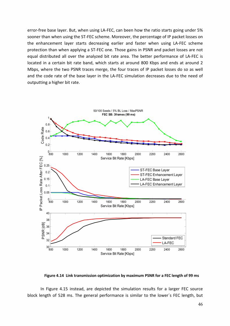
46
error-free base layer. But, when using LA-FEC, can been how the ratio starts going under 5%
sooner than when using the ST-FEC scheme. Moreover, the percentage of IP packet losses on
the enhancement layer starts decreasing earlier and faster when using LA-FEC scheme
protection than when applying a ST-FEC one. Those gains in PSNR and packet losses are not
equal distributed all over the analyzed bit rate area. The better performance of LA-FEC is
located in a certain bit rate band, which starts at around 800 Kbps and ends at around 2
Mbps, where the two PSNR traces merge, the four traces of IP packet losses do so as well
and the code rate of the base layer in the LA-FEC simulation decreases due to the need of
outputting a higher bit rate.
800 1000 1200 1400 1600 1800 2000 2200 2400 26000
0.2
0.4
0.6
0.8
1
Service Bit Rate [Kbps]
Code Rate
50/100 Seeds / 5% BL Loss / MaxPSNR
FEC SB: 3frames (99 ms)
800 1000 1200 1400 1600 1800 2000 2200 2400 26000
0.05
0.1
0.15
0.2
0.25
Service Bit Rate [Kbps]
IP Packet Loss Rate After FEC [%]
ST-FEC Base Layer
ST-FEC Enhancement Layer
LA-FEC Base Layer
LA-FEC Enhancement Layer
800 1000 1200 1400 1600 1800 2000 2200 2400 260030
32
34
36
38
40
Service Bit Rate [Kbps]
PSNR [dB]
Standard FEC
LA-FEC
Figure 4.14 Link transmission optimization by maximum PSNR for a FEC length of 99 ms
In Figure 4.15 instead, are depicted the simulation results for a larger FEC source
block length of 528 ms. The general performance is similar to the lower´s FEC length, but

47
there is a significant difference in the width of the benefit bit rate band. In this situation, the
gain is reduced to a band going from 800 Kbps to 1200 Kbps and the PSNR difference is at
most 1.5 dB. Keeping fulfilled as well the base layer packet lost constraint of a maximum of
5% IP packet loses. In this case, when the FEC source block length is equal to 528 ms, can be
seen how at 1200 Kbps, the difference between the two protection schemes is reduced to
zero in terms of PSNR and IP packet losses. From that bit rate on, the LA-FEC base layer code
rate starts decreasing not because the LA-FEC technique itself, but for the need of
outputting a high bit rate.
800 1000 1200 1400 1600 1800 2000 2200 2400 26000.2
0.4
0.6
0.8
1
Service Bit Rate [Kbps]
Code R
ate
50 Seeds / 5% BL Loss / MaxPSNR
FEC SB: 16frames (528 ms)
800 1000 1200 1400 1600 1800 2000 2200 2400 26000
0.05
0.1
0.15
0.2
Service Bit Rate [Kbps]
IP P
acket Loss R
ate A
fter FEC [%]
ST-FEC Base Layer
ST-FEC Enhancement Layer
LA-FEC Base Layer
LA-FEC Enhancement Layer
800 1000 1200 1400 1600 1800 2000 2200 2400 260032
34
36
38
40
Service Bit Rate [Kbps]
PSNR [dB]
Standard FEC
LA-FEC
Figure 4.15 Link transmission optimization by maximum PSNR for a FEC length of 528 ms

48
4.5 Code Rate Optimization by Minimum IP
Packet Loss Rate in the Enhancement Layer
Another measure for the optimization of the code rate is based on the IP packet loss
rate. That is, for a given throughput, among all the possible code rate combinations which
satisfy that throughput, the optimal chosen code rate would be the one which leads in the
minimum IP packet loss rate on the enhancement layer instead of regarding the PSNR
achieved. The base layer IP packet loss rate is already constraint to be below 5%, so the
remaining protection has to be put in such a way that the enhancement layer IP packets get
lost as low as possible.
800 1000 1200 1400 1600 1800 2000 2200 2400 26000.2
0.4
0.6
0.8
1
Service Bit Rate [Kbps]
Code R
ate
50/100 Seeds / 5% BL Loss / MinPLR-EL
FEC SB: 3frames (99 ms)
800 1000 1200 1400 1600 1800 2000 2200 2400 26000
0.1
0.2
0.3
0.4
Service Bit Rate [Kbps]
IP P
acket Loss R
ate A
fter FEC [%
]
ST-FEC Base Layer
ST-FEC Enhancement Layer
LA-FEC Base Layer
LA-FEC Enhancement Layer
800 1000 1200 1400 1600 1800 2000 2200 2400 260030
35
40
Service Bit Rate [Kbps]
PSNR [dB]
Standard FEC
LA-FEC
Figure 4.16 Link transmission optimization by minimum IP packet loss rate in the
enhancement layer for a FEC length of 99 ms

49
Regarding the results shown in Figure 4.16, it can be seen that as well as happened in
the maximum PSNR optimization, the LA-FEC brings a gain in terms of PSNR at reception and
also in IP packet loss rate over a wide range of the analyzed bit rate. The gain bit rate band in
case of a FEC source block length of 99 ms goes from 800 Kbps to 2 Mbps as happened in the
previous optimization by PSNR. But the difference arises when regarding the LA-FEC code
rates that have been selected in the optimization. In this case, the code rate of the base
layer increases faster and stays more stable while the enhancement layer code rate
decreases smoothly.
800 1000 1200 1400 1600 1800 2000 2200 2400 26000.2
0.4
0.6
0.8
1
Service Bit Rate [Kbps]
Code R
ate
50 Seeds / 5% BL Loss / MinPLR-EL
FEC SB: 16frames (528 ms)
800 1000 1200 1400 1600 1800 2000 2200 2400 26000
0.05
0.1
0.15
0.2
Service Bit Rate [Kbps]
IP P
acket Loss R
ate A
fter FEC [%
]
ST-FEC Base Layer
ST-FEC Enhancement Layer
LA-FEC Base Layer
LA-FEC Enhancement Layer
800 1000 1200 1400 1600 1800 2000 2200 2400 260032
34
36
38
40
Service Bit Rate [Kbps]
PSNR [dB]
Standard FEC
LA-FEC
Figure 4.17 Link transmission optimization by minimum IP packet loss rate in the
enhancement layer for a FEC length of 528 ms
In Figure 4.17 the same results are depicted but for a FEC source block length of 528
ms. A similar gain compared to the PSNR optimization is achieved. The main difference is
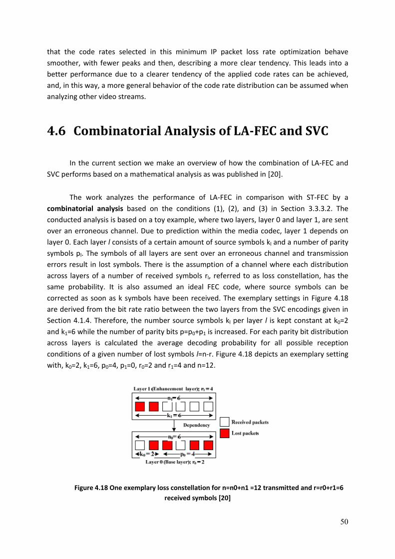
50
that the code rates selected in this minimum IP packet loss rate optimization behave
smoother, with fewer peaks and then, describing a more clear tendency. This leads into a
better performance due to a clearer tendency of the applied code rates can be achieved,
and, in this way, a more general behavior of the code rate distribution can be assumed when
analyzing other video streams.
4.6 Combinatorial Analysis of LA-FEC and SVC
In the current section we make an overview of how the combination of LA-FEC and
SVC performs based on a mathematical analysis as was published in [20].
The work analyzes the performance of LA-FEC in comparison with ST-FEC by a
combinatorial analysis based on the conditions (1), (2), and (3) in Section 3.3.3.2. The
conducted analysis is based on a toy example, where two layers, layer 0 and layer 1, are sent
over an erroneous channel. Due to prediction within the media codec, layer 1 depends on
layer 0. Each layer l consists of a certain amount of source symbols kl and a number of parity
symbols pl. The symbols of all layers are sent over an erroneous channel and transmission
errors result in lost symbols. There is the assumption of a channel where each distribution
across layers of a number of received symbols rl, referred to as loss constellation, has the
same probability. It is also assumed an ideal FEC code, where source symbols can be
corrected as soon as k symbols have been received. The exemplary settings in Figure 4.18
are derived from the bit rate ratio between the two layers from the SVC encodings given in
Section 4.1.4. Therefore, the number source symbols kl per layer l is kept constant at k0=2
and k1=6 while the number of parity bits p=p0+p1 is increased. For each parity bit distribution
across layers is calculated the average decoding probability for all possible reception
conditions of a given number of lost symbols l=n-r. Figure 4.18 depicts an exemplary setting
with, k0=2, k1=6, p0=4, p1=0, r0=2 and r1=4 and n=12.
Figure 4.18 One exemplary loss constellation for n=n0+n1 =12 transmitted and r=r0+r1=6
received symbols [20]

51
For each loss constellation is calculated the decoding probability for each layer based
on the conditions from Section 3.3.3.2. The overall number of sent packets n is increased
while keeping the number of source symbols k0 and k1 constant. The decoding probability of
each code rate distribution for each layer is calculated at a received packets value of 70%,
which corresponds to the selected average losses of 22% of the selected GE channel (see
Section 1.1). Based on these probability calculations, is selected the highest base layer code
rate giving a base layer decoding probability of 90%. Note that the highest base layer code
rate fulfilling the decoding constraint allows maximizing the protection of the enhancement
layer. The calculated optimal code rates for base and enhancement layer for ST-FEC and LA-
FEC scheme are shown in Figure 4.19. The curves show the influence of the LA-FEC on the
base layer. While for ST-FEC, the base layer code rate has to be kept constant to keep the
target base layer decoding probability of 90%, for LAFEC, the protection can be reduced. The
released bit rate can be used for a higher protection of the enhancement layer which
increases the overall performance.
0,40
0,50
0,60
0,70
0,80
0,90
1,00
1 2 3 4 5
Co
de
rate
Number of parity symbols p = p0+p1
LA-FEC Base layer
LA-FEC Enh. layer
ST-FEC Base layer
ST-FEC Enh. layer
Figure 4.19 Optimal code rate distribution at symbol loss rate of 70% and a minimum base
layer decoding probability of 90%

52
4.7 Conclusion
In the current section has been shown the performance of different parameters of
the LA-FEC protection scheme when applied to the transmission of the video stream
described in Section 4.1.4 over the Gilbert-Elliot channel analyzed in Section 4.1.2. The
Section has covered all the channel bit rate conditions going from 800 Kbps to 2.6 Mbps. The
simulation results show how for an optimization based on maximum PSNR and on minimum
IP packet losses the LA-FEC protection technique performs better than a standard FEC
algorithm. The gain changes depending on the FEC source block length chosen and on the
optimization applied, but in all cases, at least a difference of 1.5 dB is achieved and the
decrease on the IP packet losses is as well always faster when LA-FEC is used instead of a
standard FEC scheme. In the further Sections 5 and 6, the behavior of the two FEC protection
techniques will be studied on two realistic scenarios.
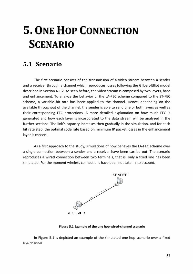
53
5. OONNEE HHOOPP CCOONNNNEECCTTIIOONN
SSCCEENNAARRIIOO
5.1 Scenario
The first scenario consists of the transmission of a video stream between a sender
and a receiver through a channel which reproduces losses following the Gilbert-Elliot model
described in Section 4.1.2. As seen before, the video stream is composed by two layers, base
and enhancement. To analyze the behavior of the LA-FEC scheme compared to the ST-FEC
scheme, a variable bit rate has been applied to the channel. Hence, depending on the
available throughput of the channel, the sender is able to send one or both layers as well as
their corresponding FEC protections. A more detailed explanation on how much FEC is
generated and how each layer is incorporated to the data stream will be analyzed in the
further sections. The link´s capacity increases then gradually in the simulation, and for each
bit rate step, the optimal code rate based on minimum IP packet losses in the enhancement
layer is chosen.
As a first approach to the study, simulations of how behaves the LA-FEC scheme over
a single connection between a sender and a receiver have been carried out. The scenario
reproduces a wired connection between two terminals, that is, only a fixed line has been
simulated. For the moment wireless connections have been not taken into account.
Figure 5.1 Example of the one hop wired-channel scenario
In Figure 5.1 is depicted an example of the simulated one hop scenario over a fixed
line channel.

54
5.2 Transmission Scheduling
Due to the losses in the channel, some parts of the video stream may get lost during
the transmission. To protect both layers of the video stream against channel errors, FEC or
LA-FEC protection is generated for each layer and it is incorporated to the transmitted bit
stream. The channel is simulated over a variable bit rate which increases gradually
providing then more throughput capacity on each increased step. Depending on the
available bit rate in the channel and as depicted in Figure 5.2, the sender is able to send the
base layer, the enhancement layer, the FEC protection for the base layer and/or the FEC/LA-
FEC protection for the enhancement layer.
Figure 5.2 Different parts of the video stream are incorporated to the transmission bit
stream depending on the available throughput
For the simulations performed, where the available bit rate of the channel increases,
the sender relies on the following transmission schedule:
- First, as soon as there is a bit rate of 164 Kbps (which is the bit rate of the base
layer) available, the base layer is transmitted
- Then, the base layer FEC protection is increased until a given condition is reached
(in this work is required that the IP packet error rate of the base layer gets to
below 1%, which entails that base layer is received quasi error-free)
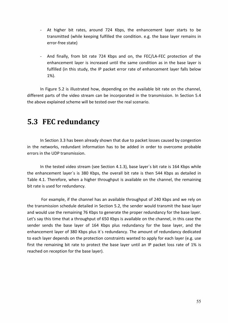
55
- At higher bit rates, around 724 Kbps, the enhancement layer starts to be
transmitted (while keeping fulfilled the condition. e.g. the base layer remains in
error-free state)
- And finally, from bit rate 724 Kbps and on, the FEC/LA-FEC protection of the
enhancement layer is increased until the same condition as in the base layer is
fulfilled (in this study, the IP packet error rate of enhancement layer falls below
1%).
In Figure 5.2 is illustrated how, depending on the available bit rate on the channel,
different parts of the video stream can be incorporated in the transmission. In Section 5.4
the above explained scheme will be tested over the real scenario.
5.3 FEC redundancy
In Section 3.3 has been already shown that due to packet losses caused by congestion
in the networks, redundant information has to be added in order to overcome probable
errors in the UDP transmission.
In the tested video stream (see Section 4.1.3), base layer´s bit rate is 164 Kbps while
the enhancement layer´s is 380 Kbps, the overall bit rate is then 544 Kbps as detailed in
Table 4.1. Therefore, when a higher throughput is available on the channel, the remaining
bit rate is used for redundancy.
For example, if the channel has an available throughput of 240 Kbps and we rely on
the transmission schedule detailed in Section 5.2, the sender would transmit the base layer
and would use the remaining 76 Kbps to generate the proper redundancy for the base layer.
Let's say this time that a throughput of 650 Kbps is available on the channel, in this case the
sender sends the base layer of 164 Kbps plus redundancy for the base layer, and the
enhancement layer of 380 Kbps plus it´s redundancy. The amount of redundancy dedicated
to each layer depends on the protection constraints wanted to apply for each layer (e.g. use
first the remaining bit rate to protect the base layer until an IP packet loss rate of 1% is
reached on reception for the base layer).

56
Variable
Throu
ghput
Affec
ted by
Losses
Gilbe
rt Elliot Channel
Figure 5.3 Example of the one hop scenario. The sender transmits a SVC stream over
channel affected by packet losses
In this scenario performing one single connection between two terminals, the sender
is aware of the throughput of the link (e.g. using a RTCP protocol as explained in [25]) and
based on that information it generates the befitting redundancy for each layer. In Section 5.4
will be detailed how the proper code rate for each layer has been chosen in case of using a
Standard FEC protection code or the LA-FEC new approach.
5.4 Simulations Results
In this section, the performance of the LA-FEC technique in the aforementioned
scenario has been analyzed over a range of service bit rate available for the inspected link
between sender and receiver going from 0 kbps to 1075 kbps. The analyzed bit rate range
shows the interesting area. That is, at higher bit rates of 1075 Kbps there is enough available
throughput to receive the video stream in perfect quality, so the interest of the study is to
analyze the bit rate area where the transition from no-video stream received to perfect
video stream received happens. The throughput range is from 164 Kbps, which is the
minimum bit rate for the base layer to be transmitted, up to 1075 Kbps where the overall
video stream becomes quasi error-free for both protection schemes.
In Section 4.2 has been already explained how the FEC source block length can be
chosen when targeting different delay video applications. Figure 4.8 shows the performance
in terms of PSNR under different FEC source block length for each protection scheme using
ST-FEC and LA-FEC. It can be seen, that a reduction of the source block length significantly
influences the protection capability of each simulated FEC scheme. Moreover, it can be seen
that the implementation of the LA-FEC protection brings a considerable gain in terms of
PSNR, either when the layers are equal or unequal error protected. For the following

57
simulations, a length of FEC source block of 16 frames has been chosen, which introduces a
delay by FEC of 0.528 s. Different FEC source block lengths may be chosen when adapting to
different delay-required systems. E.g. a FEC source block length between 0 and 150 ms
might be chosen for Video Conferencing applications. Moreover, FEC sizes of 1 to 2 sec.
would be suitable for e.g. Mobile TV systems which doesn’t require such a low delay
transmission.
The main target of video applications is to provide a stable service, e.g. a quasi error
free base layer is usually desired at reception. In this regard, a value of 1% IP packet loss rate
is the threshold that has been assumed as error free base layer in the one-hop scenario
simulations for this work.
The performed simulations show the behavior of the base and enhancement layer
depending on the bit rate available. Specifically, this work analyzes and plots for each layer
the performance of the code rates applied (Figure 5.5), the IP packet loss rate experienced in
the transmission (Figure 5.4) and the PSNR obtained in reception after the final decoding
and correction steps (Figure 5.6). Due to the higher importance of the base layer within the
SVC stream as explained in Section 3.1.3, the base layer is transmitted in first term.
Moreover, an IP packet loss rate of 1% in the base layer is the target to reach before any
attempt of transmitting the enhancement layer. As soon as there is enough bit rate
available, the enhancement layer will be transmitted and protected until the target packet
loss rate is achieved.
100 200 300 400 500 600 700 800 900 1000 11000
0.01
0.05
0.1
0.15
0.2
0.25
0.3
Service Bit Rate [Kbps]
IP Packet Loss Rate After FEC [%]
ST-FEC Base Layer
ST-FEC Enhancement Layer
LA-FEC Base Layer
LA-FEC Enhancement Layer
Figure 5.4 IP packet loss rate after decoder´s correction vs. Bit Rate available for Standard
FEC (ST-FEC) and Layer-Aware FEC (LA-FEC)

58
Regarding Figure 5.4 and Figure 5.5:
•••• Area A: Between 0 and 164 Kbps, there is not enough bit rate available to
transmit the base layer, no transmission is possible.
•••• Area B: When a bit rate of 164 Kbps is available, the transmission of the
base layer can be started. Firstly, the base layer is transmitted unprotected
due to no remaining bit rate for redundancy (Point 1). From that point on,
the more bit rate is available the more protection can be given to the base
layer. Thus, the base layer code rate is reduced until a value of 0.52 where
the target of 1% IP packet loss for the base layer is reached at bit rate 344
kbps (Point 2).
•••• Area C: Keep the sending of the base layer with 1% IP packet loss rate due
to no bit rate available to incorporate the enhancement layer in the
transmission.
•••• Area D: As soon as a bit rate of 724 kbps is ready for use, the enhancement
layer can be transmitted together with the base layer. As happened before,
first no protection is applied to the enhancement layer (Point 3).
Afterwards, gradually the code rate of the enhancement layer is reduced
until 1% IP packet loss is reached. In case of using Standard FEC scheme
protection, a bit rate of 1073 kbps is needed to fulfill the constraint of 1%
IP packet loss in the enhancement layer (Point 5). On the other hand, when
LA-FEC is used, the same constraint of packet loss is fulfilled at a bit rate of
969 kbps (Point 4), which means that LA-FEC manages to obtain a gain of
more than 100 kbps.

59
100 200 300 400 500 600 700 800 900 1000 11000.4
0.5
0.6
0.7
0.8
0.9
1
Service Bit Rate [Kbps]
Code Rate
ST-FEC Base Layer
ST-FEC Enhancement Layer
LA-FEC Base Layer
LA-FEC Enhancement Layer
No
Tranmission
Tranmission
Base LayerTranmission Base Layer with 1% IP PLR Tranmission Base Layer (1% IP PLR) +
Enhancement Layer
A CB D
1
2
5
4
3
Figure 5.5 Code rates vs. Bit Rate available for Standard FEC (ST-FEC) and Layer-Aware FEC
(LA-FEC)
Using ST-FEC, since there is no dependency within the layers, the code rate for the
base layer must be kept constant for all service bit rates to keep the IP packet error rate at
1%. Using LA-FEC, the base layer protection can be reduced due to the increasing
enhancement layer protection also protects the base layer. This translates into a PSNR gain
on the final reception and into an earlier arrival at the IP packet loss rate limit of 1%. Table
5.1 summarizes all the specific bit rate values chosen in Area D to perform the simulation as
well as the selected code rates.
Bit Rate
[kbps]
Code Rates
Standard FEC Layer-Aware FEC
Base layer Enha. Layer Base layer Enha. layer
724 0,52 1 0,52 1
782 0,52 0,88 0,54 0,86
828 0,52 0,8 0,56 0,76
869 0,52 0,74 0,58 0,68
918 0,52 0,68 0,86 0,54
976 0,52 0,62 0,94 0,5
1021 0,52 0,58 - -
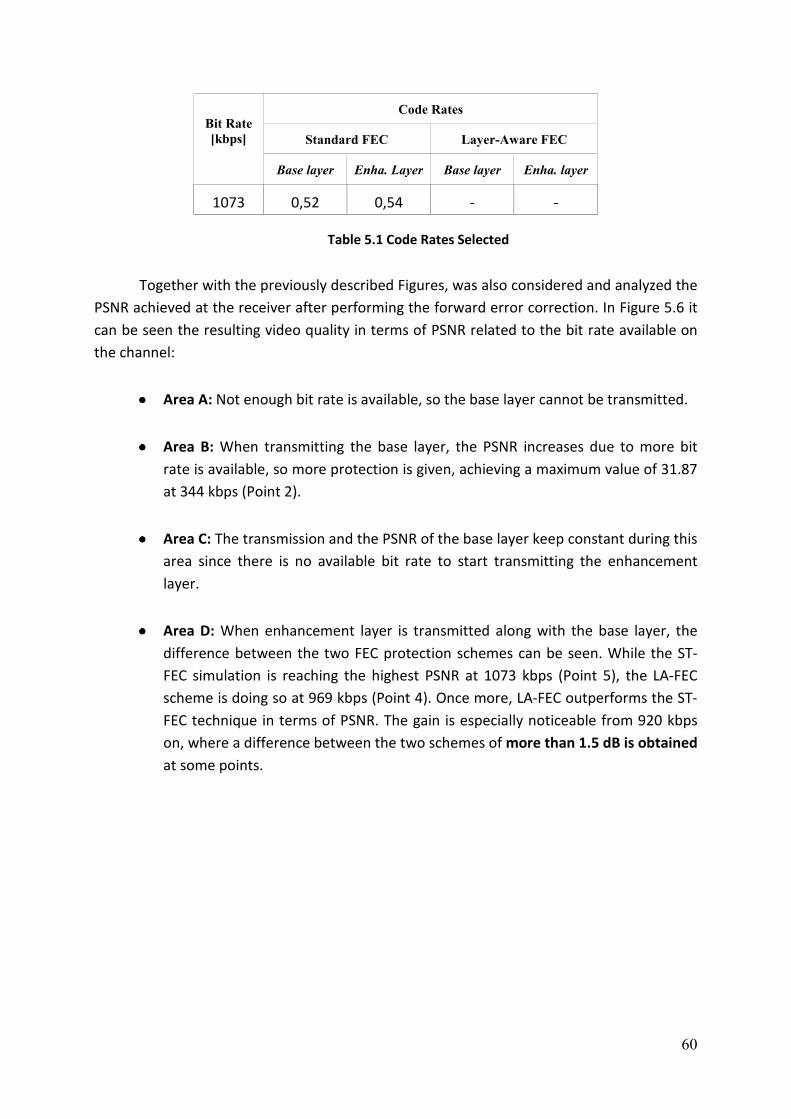
60
Bit Rate
[kbps]
Code Rates
Standard FEC Layer-Aware FEC
Base layer Enha. Layer Base layer Enha. layer
1073 0,52 0,54 - -
Table 5.1 Code Rates Selected
Together with the previously described Figures, was also considered and analyzed the
PSNR achieved at the receiver after performing the forward error correction. In Figure 5.6 it
can be seen the resulting video quality in terms of PSNR related to the bit rate available on
the channel:
•••• Area A: Not enough bit rate is available, so the base layer cannot be transmitted.
•••• Area B: When transmitting the base layer, the PSNR increases due to more bit
rate is available, so more protection is given, achieving a maximum value of 31.87
at 344 kbps (Point 2).
•••• Area C: The transmission and the PSNR of the base layer keep constant during this
area since there is no available bit rate to start transmitting the enhancement
layer.
•••• Area D: When enhancement layer is transmitted along with the base layer, the
difference between the two FEC protection schemes can be seen. While the ST-
FEC simulation is reaching the highest PSNR at 1073 kbps (Point 5), the LA-FEC
scheme is doing so at 969 kbps (Point 4). Once more, LA-FEC outperforms the ST-
FEC technique in terms of PSNR. The gain is especially noticeable from 920 kbps
on, where a difference between the two schemes of more than 1.5 dB is obtained
at some points.

61
100 200 300 400 500 600 700 800 900 1000 110024
26
28
30
32
34
36
38
40
Service Bit Rate [Kbps]
PSNR [dB]
ST-FEC
LA-FEC
Figure 5.6 PSNR vs. Bit Rate available for Standard FEC (ST-FEC) and Layer-Aware FEC (LA-
FEC)
5.5 Conclusion
In the current Section the better performance of the LA-FEC protection scheme
compared to the ST-FEC has been shown over a single connection scenario reproducing a
Gilbert-Elliot model channel covering all the channel bit rate conditions from 0 Kbps, where
no stream is transmitted, to 1075 Kbps, where both layers reach the quasi error-free state.
The results probe that LA-FEC brings a gain when base and enhancement layer are
jointly transmitted from 724 Kbps on, as theoretically explained in Section 3.3.3.2. The
results show therefore, the gain on IP packet losses and PSNR of the LA-FEC approach
compared to ST-FEC when the analyzed video stream is sent over the single hop channel
scenario. Moreover, a study of how the two FEC protection schemes behave in a more
complex scenario containing several clients with several throughputs will be detailed in
Section 6.

62
6. CCEENNTTRRAALL NNOODDEE NNEETTWWOORRKK
SSCCEENNAARRIIOO
6.1 Scenario
The second analyzed scenario is a more complex scenario in which several clients
with different throughputs and different device capacities connect to a central node that
coordinates all the participants in the transmission.
Figure 6.1 Example of the central node wired-channel scenario
A basic exemplary scheme of how the central node scenario looks is shown in Figure
6.1. Participants in the transmission who want to send or receive data connect to the central
node MANE (Media Aware Network Element) which is a network entity that is aware of the
characteristics of every client as well as the throughput available of each link. Clients
involved in the transmission are considered to have different throughput link capacities and
different terminal characteristics.
The central node collects feedback from all the connected clients by means of the
Real-Time Transport Control Protocol (RTCP) (for specific details about how the protocol
works the reader is referred to [25]). This feedback that MANE receives from the clients
includes their throughput capacity, their decoder´s complexity and the rest of information
necessary for the MANE to decide which stream is able to receive each client.
The clients are sending data over two erroneous channels which have been modeled
using the same Gilbert-Elliot channel model as described in Section 4.1.2 and used in Section
5 for the previous simulations. The channels are then reproducing packet losses. To cope

63
with such losses the sender has to apply redundancy to the data transmitted over the first
channel (connects the sender to the MANE), as well as the MANE generates the redundancy
for the data transmitted through the second hop channel (which connects the MANE with
the receiver). The mentioned redundancy is generated based on the capacity of the designed
receiver and on the characteristics of its link. In the same way as was done in the one hop
connection scenario, the redundancy is generated based on optimization criteria which will
be explained in the further sections.
6.1.1 Transmission Scheduling
The transmission schedule proposed for this scenario is the same as the one
described on the previous Section 5.2 from the one hop scenario. That schedule was
designed as follows:
� 1st base layer is sent.
� 2nd the FEC protection for base layer is applied until a quasi-error free (1% IP
packet losses) base layer is achieved.
� 3rd when enough bit rate available, the enhancement layer is sent.
� 4th the FEC for enhancement layer is transmitted until a quasi-error (1% IP
packet losses) free enhancement layer is achieved.
6.1.2 FEC redundancy
In this second modeled scenario, where a central node coordinates all the
participants, the FEC redundancy does not work in the same way as in the previous studied
scenario in Section 5. That is because in here, there are two transmission channels instead of
one. The first hop between a sender and the MANE could be considered in FEC terms like a
one hop connection as in the previous scenario. But the FEC for the second hop between
MANE and receiver results to be more complicated, in this case the MANE has to adapt the
received stream to send it over the different channels to each receiver. Adapting the
received stream consists of adding or dropping FEC protection for each layer and/or any
layer itself depending on the receiver´s link capacity, as well as selecting the proper
transmission schedule also based on the receiver´s channel characteristics.
Therefore, a more complex situation arises due to the FEC redundancy has to be
generated within two points:
� First of all, the sender generates redundancy (chooses the code rate) to send the
video stream over the link SENDER-MANE optimizing the link´s capacity.

64
� Afterwards, the MANE has to increase/reduce the received FEC protection
(change the code rate) or even drop the whole enhancement layer in order to
transmit through each second link MANE-RECEIVER depending on the receiver´s
link throughput and its terminal capacity
In this way, the sender and the MANE would transmit the two layers of the video
stream and generate the proper redundancy for each of them based on the transmission
schedule described in Section 6.1.1 and on the transmission´s link capacity.
An exemplary scenario situation is analyzed:
For instance, due to its capacity (device and link´s capacity), the sender is able to
transmit the base layer with a certain amount of protection and the enhancement layer
unprotected, which are sent through the first channel to the MANE. All the receivers have
the same throughput capacity like the sender to the MANE, i.e. the MANE would just
forward the received stream to them. Excepting one receiver that is not able enough to get
the entire stream, indeed, is only able to get the base layer. In such a case, the MANE has to
drop as much amount of information from the bit stream as needed to create a new adapted
stream which is able to be sent to the receiver. In the example the MANE would drop,
following the transmission scheduling, first the enhancement layer followed by the
protection of the base layer, and would leave only the base layer in the new adapted bit
stream which will be transmitted to the receiver with low capacity.
Moreover, not all the stream adaptations are performed in the same way, in fact,
depending on required system delay, two different kinds of applications are targeted in this
scenario:
� Low delay video streaming: for applications which require a low delay
transmission, such as videoconferencing, there is not possibility of any kind of
re-encoding of the video stream at the MANE, that is, the data received from
the sender is not decoded and encoded again before transmitting it again to
the receiver. Such an operation takes a considerable amount of time and
cannot be considered as a possible solution for our low delay scenario.
Instead, some other techniques to adapt the FEC redundancy to the receiver´s
link are used. Section 6.2.1 will describe a possible solution on how the stream
was adapted within this scenario.
� High delay video streaming: in case of applications without such strong delay
constraints in the transmission, a re-encoding process at the MANE is carried

65
out, in which the original sent source symbols are decoded and encoded again
depending on the characteristics of each receiver´s channel.
Figure 6.2 Example of central node scenario, where a media aware network element
(MANE) controls the media and FEC flows in a central node
Figure 6.2 depicts an exemplary scenario in which the sender and the MANE are
responsible to generate FEC parity to protect the transmitted data over the two erroneous
channels (SENDER-MANE and MANE-RECEIVER). Can be beheld also how different clients
with different terminals and capacities connect to the MANE and are able to receive
different parts of the video stream.
6.2 Simulated Approaches
6.2.1 Low Delay Transmission
As have been already mentioned before in Section 6.1.2, the Media Aware Network
Element (MANE) has to adapt the received bit stream to each receiver according to their
capacity and to the transmission schedule. That is, the priority schedule establishes that the
base layer is the most important part of the video stream so it must be sent in first term,
afterwards, the schedule sets that the redundant protection for the base layer is the second
priority. Next, the enhancement layer is added to the transmission followed by its
protection.

66
In Section 6.1.2 has been introduced the two main challenges of such a scenario. The
first one, when some clients are connected to the network and they cannot receive the
current stream because it overloads their capacity, and on the other hand, when some
receivers are able to take more parts than what has been sent by the sender. Therefore, the
MANE has to perform an adaptation depending on each case: add or drop parts of the
video stream.
In the first case when the video stream overloads any of the receiver’s capacity, the
MANE has to find the way to provide the most important part of the stream to the receiver,
i.e. it has to provide at least the base layer. In this way, the MANE has to extract information
concerning only the base layer from received bit stream. In the following Section 6.2.1.1 will
be explained how has been done the base layer information extraction from the
transmission bit stream when no re-encoding is allowed (low delay streaming).
Moreover, in the second case, when the MANE has to send the video stream received
from the sender to a receiver which has more throughput available than the actual received
bit rate of the video stream, the MANE is in condition to add protection to the bit stream in
order to fully exploit the available link´s capacity. This case is solved in a very simple way,
which is done just by adding new redundant FEC symbols to the already received encoded
symbols. Because of the encoded symbols are a linear combination of the base and the
enhancement layer symbols (as will be explained in Section 6.2.1.1), carrying out a linear
combination of the encoded symbols will lead in new encoded symbols which are also valid
for the decoder.
In order to study the source symbol encoding and extraction process, a Luby
Transform (LT) linear code [16] has been simulated. When using a LT linear code, the
encoded LT symbols become just a linear combination of the base layer and the
enhancement layer symbols. Figure 6.3 shows an example of how the LT symbols are
generated using a matricial representation (more details will be explained in Section 6.2.1.1).
The symbols marked as base layer symbols include already the redundant symbols for that
layer which have been generated before. The same applies to the enhancement layer.
6.2.1.1 Extraction of Base Layer Symbols
It has been introduced in Section 6.1.2 the need of extracting the base layer
information within the MANE in case of any receiver is not able to receive the enhancement
layer or too much FEC protection data for the base layer.

67
Figure 6.3 LT Encoding Matrix
In order to study the base layer symbol extraction a Luby Transform (LT) encoding
process [16] has been simulated. The LT encoder can be represented by an encoding matrix
(Figure 6.3) in which each row corresponds to one encoded symbol, yi, and each column to
one source symbol. The base layer symbols are named bi, while the enhancement layer
symbols ei. Each row of the matrix (which represents an encoded symbol) consist of a certain
amount of ‘1’, each of these ones indicates that the corresponding source symbol is part of
the XOR combination to generate the encoded symbol.
For instance, in the exemplary matrix shown in Figure 6.4, the first encoded symbol
y1, which is represented as the first row of the matrix, is generated by XORing the source
symbols b1, b4, b5 and e2, e3, e4, which are depicted with a ‘1’ in the corresponding column
below each source symbol. For deeper information about how to the LT matrix works refer
to [16] and [24].
In this way, it can be easily deduced that extracting new base layer encoded symbols
from LT encoded symbols could be achieved by combining, through XOR operations,
different LT symbols until a symbol with no connections to the enhancement layer source
symbols is obtained. An example of how one of this enhancement-layer-free symbols (or
base layer encoded symbol) can be extracted is depicted in Figure 6.4. Therefore, those new
extracted encoded base layer symbols contain only base-layer-related information, and can
be forwarded to the receivers with no capacity to get the enhancement layer.

68
The aforementioned idea of combining LT encoded symbols at one intermediate node
to obtain new encoded symbols, which hold also source information and are still able to be
decoded as if they were encoded in the source, have been done similarly to the research
work carried out in [21], [22] and [23].
Figure 6.4 Example of the extraction of one base layer new encoded symbol combining 3 LT
regular symbols
The most important and difficult issue of this encoded base layer symbol extraction
scheme consists of choosing properly the LT symbols which have to be combined. Clearly,
not all the combinations lead into an enhancement-layer-free-connection symbol, only
combining the proper LT symbols, a base layer encoded symbol can be obtained. Moreover,
not only which specific symbols have to be XORed is a complex step, but also how many of
them will be involved in the XOR operation is a very important issue to decide. In this work,
three different algorithms to perform the base layer symbol extraction have been tried. As a
first step, a reiterative combination of all the LT symbols is carried out. Afterwards, a random
LT symbol selection approach is used followed in the end by a pseudo reiterative algorithm
which resulted to have the best performance.
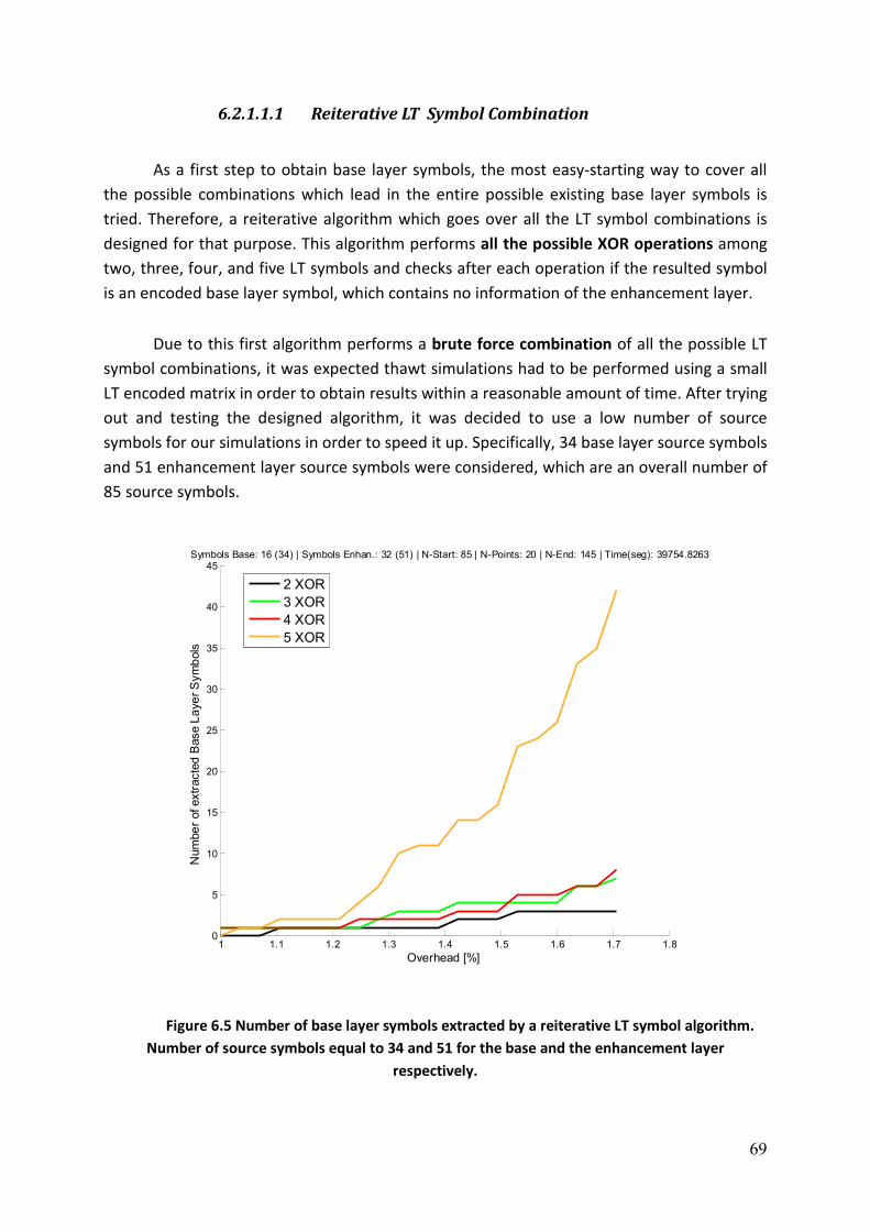
69
6.2.1.1.1 Reiterative LT Symbol Combination
As a first step to obtain base layer symbols, the most easy-starting way to cover all
the possible combinations which lead in the entire possible existing base layer symbols is
tried. Therefore, a reiterative algorithm which goes over all the LT symbol combinations is
designed for that purpose. This algorithm performs all the possible XOR operations among
two, three, four, and five LT symbols and checks after each operation if the resulted symbol
is an encoded base layer symbol, which contains no information of the enhancement layer.
Due to this first algorithm performs a brute force combination of all the possible LT
symbol combinations, it was expected thawt simulations had to be performed using a small
LT encoded matrix in order to obtain results within a reasonable amount of time. After trying
out and testing the designed algorithm, it was decided to use a low number of source
symbols for our simulations in order to speed it up. Specifically, 34 base layer source symbols
and 51 enhancement layer source symbols were considered, which are an overall number of
85 source symbols.
1 1.1 1.2 1.3 1.4 1.5 1.6 1.7 1.80
5
10
15
20
25
30
35
40
45
Overhead [%]
Number of extracted Base Layer Symbols
Symbols Base: 16 (34) | Symbols Enhan.: 32 (51) | N-Start: 85 | N-Points: 20 | N-End: 145 | Time(seg): 39754.8263
2 XOR
3 XOR
4 XOR
5 XOR
Figure 6.5 Number of base layer symbols extracted by a reiterative LT symbol algorithm.
Number of source symbols equal to 34 and 51 for the base and the enhancement layer
respectively.

70
In Figure 6.5 is shown one of the outcoming results of the applied algorithm to the LT
encoder matrix formed by 85 source symbols (34 of the base layer plus 51 of the
enhancement layer). The Figure depicts for 2, 3, 4 and 5 LT symbol XOR combinations, the
number of extracted encoded base layer symbols depending on the overhead (parity)
applied to the original source symbols. An overhead equal to 1 means that only a number of
LT symbols equal to the overall number of source symbols are generated, in this simulation
would result to 85 LT encoded symbols. When the overhead gets higher, a larger amount of
encoded LT symbols are generated, and then, the encoded matrix results to have more rows,
which leads into a higher probability to extract a base layer encoded symbol due to more
rows can be combined, so more combinations are possible.
Regarding the Figure 6.5, it can be seen how performing XOR operations between 2,
3, and 4 LT symbols the algorithm couldn’t even manage to get the same amount of original
base layer symbols (which are 34) with an overhead (or parity symbols) of 70% (point shown
as 1.7 in the X-axis of the Figure). Does not happen the same when a larger number of
symbols are XORed, performing XOR operations among 5 LT symbols the algorithm extracts
34 different encoded base layer symbols applying an overhead of around 68%, which
anyway, is still a quite big overhead.
It can be concluded that the extraction of base layer symbols from the XOR
combination of encoded LT symbols is viable. But as have been shown, if a systematic
algorithm based on brute force is used, it requires a quite high overhead protection. And
when a larger amount of source symbols is used, it entails as well, a huge amount of time. It
is because of these reasons that another algorithm will be tried with the aim of reducing
either the time employed or the overhead required, or even more, hopefully both of them.
6.2.1.1.2 Random LT Symbol Combination
As a second step in the base layer symbol extraction, a random based algorithm has
been used. This algorithm, instead of going through all the possible LT symbol combinations,
selects randomly 2, 3, 4, or 5 LT symbols and combines them with a XOR operation. The
number of times that the random loop selection is done is controlled by the parameter
NumberCombinations. Afterwards, the resulting symbol is checked in order to see if it is a
base layer encoded symbol or not, and is stored if needed.
In Figure 6.6 are depicted the simulation results when running the random LT symbol
combinator over a number of 34 base layer and 51 enhancement layer source symbols, and
a number of combinations equal to 1000000. It can be seen how using the random scheme,
and in the opposite way as happened with the previous algorithm, a higher number of base
layer symbols are obtained when a lower number of XOR combinations are performed.
However, due to the algorithm is based in randomness; the number of extracted base layer

71
symbols is much more irregular. It has an increasing trend, but depending on the random
seed, different peaks can be noticed at some overhead points. Anyway, it can be seen that
not even using a high overhead of 300% (point shown as 3 in the X-axis of the Figure 6.6) the
algorithm is able to obtain at least the 34 base layer initial source symbols.
1 1.5 2 2.5 30
1
2
3
4
5
6
7
8
9
Overhead [%]
Number of extracted Base Layer Symbols
Symbols Base: 16 (34) | Symbols Enhan.: 32 (51) | N-Start: 85 | N-Points: 20 | N-End: 255 | #Combi: 1000000 | Seed: 3 | Time(seg): 834.4722
2 XOR
3 XOR
4 XOR
5 XOR
Figure 6.6 Number of base layer symbols extracted by a random LT symbol algorithm.
Number of source symbols equal to 34 and 51 for the base and the enhancement layer
respectively.
Running the simulation with the same parameters but changing only in this case the
number of source symbols to 14 and 21 for the base and the enhancement layer
respectively, the algorithm managed to obtain better results. As can be seen in Figure 6.7, a
low overhead compared to the one needed in 6.2.1.1.1, around 60%, is required to extract at
least a number of 14 source symbols with 4 XOR combinations (red curve in the Figure 6.7).
From the simulation results, it can be deduced that when a higher amount of source
symbols is used, it becomes more critical the extraction of base layer encoded symbols from
the encoded LT symbols, needing higher overhead and larger amount of time. In the
following Section 6.2.1.1.3 a different third algorithm will be tried out.

72
1 1.5 2 2.5 30
5
10
15
20
25
30
X: 1.6Y: 13
Overhead [%]
Number of extracted Base Layer Symbols
Symbols Base: 4 (14) | Symbols Enhan.: 8 (21) | N-Start: 35 | N-Points: 20 | N-End: 105 | #Combi: 1000000 | Seed: 3 | Time(seg): 938.9991
2 XOR
3 XOR
4 XOR
5 XOR
Figure 6.7 Number of base layer symbols extracted by a random LT symbol algorithm.
Number of source symbols equal to 14 and 21 for the base and the enhancement layer
respectively.
6.2.1.1.3 Pseudo-Reiterative LT Symbol Combination
After having experienced no good enough results in terms of overhead and time
consumed with the two previous analyzed algorithms, it has been decided to implement a
pseudo-reiterative XOR combinatory algorithm, which basically consist of a reiterative brute
force algorithm but constrained by some bounds with limit the number of analyzed
combinations. This algorithm works based on two input parameters, MaxSteps and
MaxCombinations, which define the maximum number of LT symbols that are involved in
the XOR operation and the number of times that a new symbol is picked in case of the
previous XORed symbols do not lead in a base layer symbol, respectively. The LT pseudo-
systematic combinator works according to the following algorithm:
MatrixLT = (rowsLT,columnsLT) for row=1:rowsLT

73
for combinations=1:MaxCombinations for step=1:MaxSteps Best = Check_the_row_with_the_best_match(MatrixLT,row) TempRow=XOR(row,Best) if TempRow == BaseLayerSymbol Solution = [Solution ; TempRow]
Taking a look at Figure 6.8 can be seen how better results compared to the two
previously tried algorithms are obtained. In this case, the algorithm is able to extract 34 base
layer encoded symbols with an overhead of only 25% and within a very reasonable amount
time.
1 1.1 1.2 1.3 1.4 1.5 1.6 1.710
20
30
40
50
60
70
80
X: 1.25Y: 35
Overhead [%]
Number of extracted Base Layer Symbols
Symbols Base: (34) | Symbols Enhan.: (51) | Max Steps: 20 | Max Combinations: 10 | Time(seg): 4204.7312
Figure 6.8 Number of base layer symbols extracted by a pseudo-systematic LT symbol
algorithm
Now that the third tried algorithm managed to obtain, with a reasonable overhead, at
least the same number of base layer source symbols, it has to be assured that the new
obtained base encoded LT symbols are still valid for a standard LT decoder.

74
The next step is, then, to introduce those new extracted LT base layer symbols into a
LT decoder and check if they can be decoded to obtain some of the source base layer
symbols.
6.2.1.2 Simulation Results
Despite the good results obtained regarding that it has been proved that the base
layer symbol extraction is possible from LT encoded symbols, and can be done within a
reasonable amount of time and with a quite contained overhead in case of using the third
explained algorithm in Section 6.2.1.1.3, and after several different tried decoders and
overhead protections, the performed tests could not manage to get decoded those new
base layer symbols when putting them as the input of a standard LT decoder. Unfortunately,
a more deep research about this topic has to be done to assure that the extracted base layer
symbols are full-valid LT symbols and can be decoded properly as if they were encoded with
a normal LT encoder.
6.2.1.3 Conclusion
After studying the simulation results for the Low Delay Transmission scenario, it has
been concluded that the base layer encoded symbol extraction is possible from the
combination of LT encoded symbols. However, those extracted symbols cannot be decoded
within a standard LT decoder. Therefore, a deeper study in this field would be required in
order to continue with the low delay scenario simulations.
6.2.2 High Delay Transmission
In this Section the work analyzes the behavior of the central node scenario when a
high delay is permitted in the video transmission. That is, there is no need of any kind of
symbol extraction by the scheme described in Section 6.2.1. In such a high delay scenario, it
can be assumed, that the LT encoded symbols are decoded within the MANE central node
and then, encoded again to be transmitted to each of the receivers.
In this way, the simulation of the scenario was performed based on what was done in
the one hop connection transmission described in Section 5 but just considering one more
transmission hop. The central node network simulator (which is designed as the one
depicted in Figure 6.2) can be configured for different number of clients which connect to
the MANE, and each client can be set up with the desired throughput available.

75
Furthermore, any of the connected nodes can be selected as the server node, which sends
the video stream.
The simulator starts by optimizing the link Sender-MANE in terms of maximum PSNR
based on all the simulation data files whose code rates are depicted in the previously
explained Figure 4.12 (if the FEC source block length chosen is 99 ms) and Figure 4.13 (for a
FEC source block length of 528 ms). In this case, an optimization based on maximum PSNR
has been chosen due to the simplicity of comparing the quality at reception on each receiver
when a large amount of receivers are simulated. Even though the optimization based on
maximum PSNR is not the best choice when comparing video streaming quality, it is a good
enough solution for a precise idea of how a scenario, such the one in the current Section 6,
behaves when different FEC protection schemes are applied.
Afterwards, once the optimal code rate for the sender´s throughput is chosen and the
simulation transmission for the first hop Sender-MANE is completed, the proper code rate
selection needs to be determined at the MANE for both, base and enhancement layer. The
selected code rates at the MANE are dependent on what was sent by the server and on the
FEC scheme applied. For instance, if the sender is only able to send the base layer there is no
way to provide the enhancement layer to the receivers.
6.2.2.1 Simulation Results
The code rate optimization for each receiver has been optimized based on the
maximum PSNR at reception. That is, among all the possible code rate protections that each
client is able to receive, the chosen one is the one which leads into the higher PSNR at
reception.
The simulations are carried out considering that different nodes with different
throughputs are connected to the central node. After this, the simulator performs as many
simulations as number of nodes exist. In each simulation the sender node is changed and the
experienced PSNR of each of the receiver nodes is calculated. Due to the nodes have
different throughputs, depending on which node sends the data and on its capacity, the
receiver nodes can get or not the entire stream.
In Figure 6.9 can be seen the results of the simulation for a number of 9 nodes
connected to the MANE. The nine nodes have the different throughput, which are equal to
700, 750, 800, 850, 900, 950, 1000, 1050 and 1100 Kbps. Each of the subplots represented in
Figure 6.9 corresponds to the PSNR achieved at each of the receivers when the different
nodes behave as the sender node.

76
Note that, as well as was explained in Section 5, the minimum bit rate capacity of
each link that have been taken into account is the one needed to send the base layer in
quasi error-free state (1% losses in the base layer), which is, as seen in Section 5, 344 Kbps.
From that bit rate point up to 724 Kbps, where the sender is able to send the enhancement
layer without protection (cf. Section 5.4), there is a bit rate area in which the PSNR that any
node can achieve is equal to 32 dB, which is the PSNR of getting the base layer in quasi-error
free state, stands the same as seen in Section 5.4 for one single hop connection.
In the first subplot in Figure 6.9, when the sender node is the node 1, can be seen
how the rest of the nodes cannot get more than the base layer due to node 1 has capacity
only to send the base layer (Link Node 1 -> Mane: 700 Kbps). That means, the maximum
achievable video quality is 32 dB for both, LA-FEC and ST-FEC, protection schemes.
Moreover, regarding to the fifth subplot in Figure 6.9, where the sender node is the
node 5 (Link Node 5 -> Mane: 900 Kbps), the difference between the two protection
schemes, ST-FEC and LA-FEC, is noticeable. In this case, the PSNR quality at reception using a
ST-FEC scheme is almost 36 dB for the nodes 5-9, while for the same nodes when using a LA-
FEC scheme, it is almost 38 dB. It can be seen as well, that the PSNR for the nodes 1 and 2 is
equal independent of the FEC protection scheme. That is because those nodes have not
enough link capacity to get more than the base layer quasi error-free, so their PSNR achieved
at reception cannot get more than 32 dB even though the sender is able to send the
enhancement layer as well.
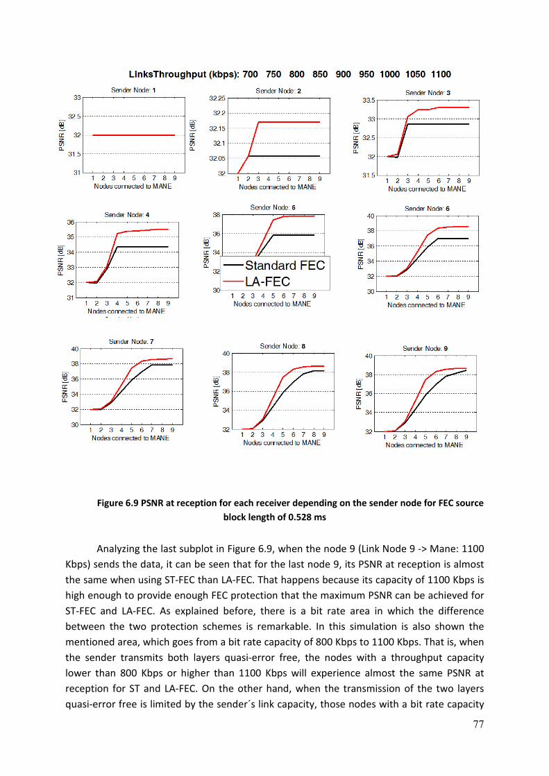
77
Figure 6.9 PSNR at reception for each receiver depending on the sender node for FEC source
block length of 0.528 ms
Analyzing the last subplot in Figure 6.9, when the node 9 (Link Node 9 -> Mane: 1100
Kbps) sends the data, it can be seen that for the last node 9, its PSNR at reception is almost
the same when using ST-FEC than LA-FEC. That happens because its capacity of 1100 Kbps is
high enough to provide enough FEC protection that the maximum PSNR can be achieved for
ST-FEC and LA-FEC. As explained before, there is a bit rate area in which the difference
between the two protection schemes is remarkable. In this simulation is also shown the
mentioned area, which goes from a bit rate capacity of 800 Kbps to 1100 Kbps. That is, when
the sender transmits both layers quasi-error free, the nodes with a throughput capacity
lower than 800 Kbps or higher than 1100 Kbps will experience almost the same PSNR at
reception for ST and LA-FEC. On the other hand, when the transmission of the two layers
quasi-error free is limited by the sender´s link capacity, those nodes with a bit rate capacity

78
included between the bit rate values of 800 Kbps and 1100 Kbps, will manage to have better
PSNR at reception when using a LA-FEC protection scheme, than when using a ST-FEC
technique.
6.3 Summary of Section 6
The current section studies the behavior of the two FEC protection techniques
applied to a central node scenario in which several clients with different device capabilities
and different throughput capacities exchange information through the so-called central
node MANE which is aware of each device´s characteristics. Depending on the required
delay in the system two different kinds of applications can be targeted, low and high delay
video transmission.
Concerning the low delay transmission scenario arises the need of extracting encoded
symbols containing information related only to the base layer due to the lack of time to re-
encode the video stream for the clients with lower capacity. Those symbols are used to be
sent over the receiver´s links with not enough capacity to get the full video stream.
Simulations have shown how the extraction of the symbols is possible using a combinatorial
algorithm. However, the proper decoding of the symbols could not be achieved by means of
the studied LT decoders. Therefore, results regarding the PSNR at reception of each of the
receivers could not be obtained due to the lack of a full working base layer symbol extractor
at the MANE.
On the other hand, a high delay transmission scenario has been simulated for those
applications in which the delay is not a restrictive constraint. In such a scenario, the LT
symbols sent over the first link Sender -> MANE are re-encoded again within the central
node. Hence, a new FEC redundancy can be applied to each of the layers at the MANE
adapting the video stream to each receiver´s capacity. Simulations have shown how
depending on the sender´s link capacity, the different receivers can achieve a gain in terms
of PSNR and IP packet loss rate at reception when using a LA-FEC protection scheme instead
of a traditional FEC technique.
79
7. CCOONNCCLLUUSSIIOONNSS AANNDD FFUUTTUURREE
WWOORRKK The present Master Thesis tackles video transmission solutions over a channel
without QoS. These channels are especially sensitive to packet losses, and moreover, this
becomes more critical when layered media such as SVC is applied. To cope with these
channel errors, FEC protection techniques can be used. This work compares a standard FEC
scheme (ST-FEC) and the Layer-Aware FEC (LA-FEC) approach when transmitting a SVC
stream over an error prone channel in two different scenarios.
The difference between ST-FEC and LA-FEC has been analyzed on a first simple
scenario, where a single hop connection between two clients over a Gilbert-Elliot channel is
simulated for different throughput link capacities. For each bit rate link capacity point, an
optimization based on maximum PSNR and minimum IP packet lost rate in the enhancement
layer has been performed. Simulation results show how by means of a ST-FEC scheme, since
there is no dependency within the layers, the code rate for the base layer must be kept
constant for all service bit rates to assure a quasi-error free base layer at reception. Instead,
when a LA-FEC protection scheme is applied, the base layer protection can be reduced due
to the increasing enhancement layer protection also protects the base layer. This translates
into a PSNR gain on the final reception and into an earlier arrival at the IP packet loss rate
limit of 1% (or quasi-error free) for both layers.
Furthermore, on the second considered scenario with multiple clients connected
through a central node, two delay cases have been analyzed depending on the targeted
video application.
On the one hand, a low delay system has been considered, in which a re-encoding
process of the video stream cannot be carried out within the central node (Media Aware
Network Element) in order to keep the end-to-end latency of the system low. In this regard,
another solution to adapt the received stream in the MANE to the characteristics of each
receiver is proposed: combine the encoded symbols which compose the video stream (or LT
symbols) in order to extract new encoded symbols containing information related only to
the most important layer, the base layer.
It has been shown how the extraction of those new encoded symbols containing
information only of the base layer, through the combination of regular encoded LT symbols,
is possible. However, those new extracted encoded base layer symbols could not be properly
decoded with a standard LT decoder.

80
On the other hand, when a high delay is permitted in the transmission, a re-encoding
process is performed within the central node. The new encoding process of the stream at
the MANE, allows that new FEC redundancy can be applied to each layer optimizing each
receiver´s capacity. Simulations have shown how those clients, whose available throughput
is contained in a certain bit rate area (which is related to the sent video stream), are able to
achieve a significant gain in terms of PSNR at reception thank to the usage of the LA-FEC
protection scheme.
The developed work in this Thesis can be used as excellent basis to further
investigations related to specific topics that have been introduced here. In this regard, would
be very interesting the development of this study for several different video streams with
the aim of finding out a formula which empirically summarizes the code rate optimal
distribution depending on the bit rate of the video stream as well as on the available
throughput in the connection link.
In a similar way, a study of how the LA-FEC scheme behaves over different channels,
with different loss patterns, would be desirable in order to deduce the influence of the
channel on the encoder´s code rate optimization.
Besides, regarding the low delay case into the central node scenario, a deeper
research, covering the LT encoding matrix and the different LT decoders, would be required
to achieve the proper decoding of the new extracted base layer symbols.
81
8. CCOONNCCLLUUSSIIOONNEESS YY TTRRAABBAAJJOO
FFUUTTUURROO El presente Proyecto Final de Carrera aborda soluciones para la transmisión de vídeo
codificado a través de canales sin Calidad de Servicio (QoS). Estos canales son especialmente
sensibles a las pérdidas de paquetes, y además, las pérdidas se vuelven más críticas cuando
se trata de una transmisión de vídeo por capas (Scalable Video Coding). Para hacer frente a
estos errores del canal se pueden aplicar técnicas FEC de corrección de errores. Este trabajo
compara una técnica FEC estándar de protección de errores (ST-FEC) con el nuevo esquema
de protección Layer-Aware FEC (LA-FEC) cuando se transmiste un flujo de datos de vídeo
escalable codificado (Scalable Video Coding) a través de un canal erróneo en dos escenarios
diferentes.
La diferencia entre las técnicas ST-FEC y LA-FEC ha sido analizada en un primer
escenario simple, dónde se simula una conexión entre dos clientes a través de un canal
siguiendo el módelo de Gilbert-Elliot para diferentes capacidades de ancho de banda. Para
cada ancho de banda simulado se ha llevado a cabo una optimización basada en el máximo
PSNR en recepción y en la mínima tasa de pérdida de paquetes IP (Internet Protocol) en la
capa de mejora (enhancement layer). Los resultados de las simulaciones muestran como
usando una técnica ST-FEC, debido a que no hay interdependencia entre las capas, la tasa de
protección para la capa base (base layer) debe mantenerse constante para todos los anchos
de banda de servicio con el fin de asegurar que la capa base se recibe cuasi libre de errores.
En cambio, cuando aplicamos la técnica de protección LA-FEC, la tasa de protección para la
capa base puede ser reducida gracias a que el aumento de protección en la capa de mejora
protege también la capa base. Esto se traduce en una ganancia en la relación Señal a Ruido
de pico (PSNR) en la recepción final y en un llegada más rápida al límite de 1% de tasa de
pérdida de paquetes IP (o cuasi libre de errores) para ambas capas.
Más adelante, en el segundo escenario analizado, dónde varios clientes están
conectados a través de un nodo central, hemos diferenciado dos casos dependiendo del
retardo requerido para la aplicación de vídeo.
Por un lado hemos considerado un escenario con bajo nivel de retardo, en el cual un
proceso de re-codificación del flujo de datos de vídeo no puede ser llevado a cabo dentro del
nodo central (MANE) con el fin de mantener la latencia extremo a extremo del sistema baja.
Con este propósito, se ha propuesto otra solución para adaptar el vídeo recibido en el MANE
a las características de cada receptor: combinar los símbolos codificados que componen el
flujo de datos de vídeo (ó símbolos LT) con el objetivo de extraer nuevos símbolos

82
codificados que contengan información relacionada sólo con la capa más importante, la capa
base.
Se ha mostrado cómo la extracción de esos nuevos símbolos codificados que
contienen sólo información de la capa base, a través de la combinación de símbolos LT
codificados normales, es posible. Sin embargo, esos símbolos codificados extraídos con
información de la capa base no pudieron ser correctamente decodificados con un
decodificador LT estándar.
Por otro lado, cuando consideramos un escenario con retardo permitido alto, un
proceso de re-codificación del flujo de datos de vídeo es llevabo a cabo en el nodo central. El
nuevo proceso de codificación del flujo de datos en el MANE permite que se pueda aplicar
una nueva tasa de protección a cada capa optimizando la capacidad de ancho de banda de
cada cliente receptor. Las simulaciones han mostrado cómo aquellos clientes cuyo ancho de
banda disponible está contenido en un cierto rango (el cúal está relacionado con la tasa de
codificación del video enviado), son capaces de alcanzar una ganancia significativa en
términos de Señal a Ruido de pico (PSNR) en la recepción gracias al uso del esquema de
protección LA-FEC.
El trabajo desarollado en este Proyecto Final puede ser usado como una excelente
base para futuras investigaciones relacionadas con los temas específicos que han sido
introducidos aquí. En relación con lo mencionado, sería muy interesante el desarrollo de
este mismo estudio para diferentes fragmentos de vídeo con el objetivo de encontrar una
fórmula que empíricamente resuma la distribución óptima de la tasa de protección aplicada
a cada capa dependiendo de la tasa de codificación del video transmitido y del ancho de
banda disponible en el canal.
De una manera similar, un estudio de cómo el esquema LA-FEC se comporta para
diferentes canales, con diferentes patrones de pérdidas, sería deseable con el fín de deducir
la influencia del canal en la optimización de la tasa de protección en el codificador.
Por otro lado, con respecto al caso de bajo nivel de retardo en el escenario con nodo
central, una investigación más profunda, contemplando la matriz de codificación LT y los
diferentes decodificadores LT, sería requerida para alcanzar la correcta decodificación de los
nuevos símbolos extraídos con información relacionada sólo con la capa base.

83
84
RREEFFEERREENNCCEESS [1] Ahmed Abad. “Video compressing techniques”, www.sigmatrainers.com, India
[2] Susanna Spinsante, Ennio Gambi, Lorenzo Ciccarelli, Andrea Lorenzo Vitali, Jorge
Sastre Martínez, and Paul Salama. “Advances in Video Coding for Broadcast
Applications”, International Journal of Digital Multimedia Broadcasting, vol. 2009,
Article ID 368326, 2 pages, 2009. doi:10.1155/2009/368326.
[3] Heiko Schwarz, Detlev Marpe and Thomas Wiegand. “Overview of the
Scalable Video Coding. Extension of the H.264/AVC Standard. IEEE
Transactions on circuits and systems for video technology, Vol 17, No. 9,
September 2007.
[4] N.S.Narkhede and Naveeta Kant. “The emerging h.264/advanced video
codingstandard and its applications”. International conference on advances in
computing, communication and control. India, January 2009.
[5] Iain Richardson. “White paper: An overview of the H.264 advanced video
coding”. Vcodex, 2007
[6] Ralf Schäfer, Thomas Wiegand and Heiko Schwarz. “The emerging h.264/AVC
standard”. Heinrich Hertz Institute, Berlin, Germany.
[7] T. Wiegand, G. J. Sullivan, G. Bjøntegaard, and A. Luthra. “Overview of the
H.264/AVC video coding standard”, IEEE Trans. Circuits Syst. Video Technol.,
vol. 13, no. 7, pp. 560–576, Jul. 2003.
[8] “Advanced Video Coding for Generic Audiovisual Services”. ITU-T Rec. H.264
and ISO/IEC 14496-10 (MPEG-4 AVC), ITU-T and ISO/IECJTC 1, Version 1: May
2003, Version 2: May 2004, Version 3: Mar.2005, Version 4: Sept. 2005,
Version 5 and Version 6: June 2006, Version7: Apr. 2007, Version 8 (including
SVC extension): Consented in July 2007.
[9] Image communication group, Fraunhofer Heinrich Hertz Institute. “The
Scalable Video Coding Amendment of the H.264/AVC Standard”.
[10] Thomas Wiegand, Ludovic Noblet and Fabrizio Rovati. “Scalable video coding
for IPTV services”. IEEE Transactions on broadcasting. Vol 55, No 2, June 2009.

85
[11] Wikipedia – ”Internet Protocol”
[12] Wikipedia – ”User Datagram Protocol”
[13] Wikipedia – ”Error detection and correction”
[14] AERO.org – “How Forward Error-Correcting Codes Work”
[15] Image communication group, Fraunhofer Heinrich Hertz Institute. “Layer-
Aware Forward Error Correction (L-FEC)”
[16] M. Luby. “LT-codes”, in Proc. 43rd Annu. IEEE Symp. Foundations of Computer
Science (FOCS), Vancouver, BC, Canada, Nov. 2002, pp. 271–280
[17] Amin Shokrollahi, “Raptor Codes”, IEEE Transactions on Information Theory,
vol. 52, pp. 2551-2567, 2006
[18] V. Markovski, F. Xue, and L. Trajkovic. “Simulation and analysis of packet loss
in user datagram protocol transfers,” The Journal of Supercomputing, Vol. 20,
No. 2, September 2001.
[19] ITU-T: ITU Recommendation G. 114, Series G: Transmission Systems and
Media, Digital Systems and Networks, May, 2003.
[20] Cornelius Hellge, David Gómez-Barquero, Thomas Schierl and Thomas
Wiegand. “Layer-Aware forward error correction for mobile broadcast of
layered media”, IEEE Circuits & Systems Society, March 2011.
[21] Nikolaos Thomos and Pascal Frossard. “Raptor Network Video Coding”.
MV´07, Augsburg, Bavaria, Germany, September 2007.
[22] Nikolaos Thomos, Jacob Chakareski and Pascal Frossard. “Randomized
Network Coding for UEP video delivery in overlay networks”. ICME 2009.
[23] Enrico Magli and Pascal Frossard. “An overview of network coding for
multimedia streaming”. ICME 2009.
[24] Sheng-Kai Chang, Kai-Chao Yang, and Jia-Shung Wang. “Unequal-Protected LT
Code for layered video streaming”. Proceedings of IEEE International
Conference on Communications, ICC 2008, Beijing, China, 19-23 May 2008

86
[25] Standard Tracks. “RTP: A Transport Protocol for Real-Time Applications” , RFC
3550. July 2003
[26] The PERL Programming Language. www.Perl.org
[27] MATLAB – The Language of Technical Computing. www.mathworks.com

i
GGLLOOSSSSAARRYY RGB – Red Green Blue
Is an additive color model in which red, green, and blue light are added together in
various ways to reproduce a broad array of colors.
FEC - Forward Error Correction
Is a system of error control for data transmission, whereby the sender adds
systematically generated redundant data to its messages. The redundant data allows the
receiver to detect and correct possible errors in the received data. The main advantage
of this error control technique is the no need of any retransmission from the sender.
ARQ - Automatic Repeat Request
Is an error-control method for data transmission that uses acknowledgements
(messages sent by the receiver indicating that it has correctly received a data frame or
packet) and timeouts (specified periods of time allowed to elapse before an
acknowledgment is to be received) to achieve reliable data transmission over an
unreliable service.
Media Streaming
Is multimedia that is constantly received by and presented to an end-user while being
delivered by a streaming provider.
MANE
Stands for Media Aware Network Element. Is a network entity that is aware of the
characteristics of every client as well as the throughput available of each link.
H.264/AVC
Advanced Video Coding Standard.

ii
SVC - Scalable Video Coding
Is the name for the Annex G extension of the H.264/MPEG-4 AVC video compression
standard. SVC standardizes the encoding of a high-quality video bit stream that also
contains one or more subset bit streams.
DVB - Digital Video Broadcasting
Is a suite of internationally accepted open standards for digital television.
GOP - Group of Pictures
In video coding, a group of pictures, or GOP structure, specifies the order in which intra-
and inter-frames are arranged. The GOP is a group of successive pictures within a coded
video stream. Each coded video stream consists of successive GOPs. From the pictures
contained in it, the visible frames are generated.
DP - Dependency Path
A dependency path (DP) includes, for a particular frame, all the referenced layers in the
order of importance.
CIF - Common Intermediate Format
A set of standard video formats used in videoconferencing, defined by their resolution.
The original CIF is also known as Full CIF (FCIF).
QCIF
Quarter resolution of a CIF
MPEG-1
Is a standard for lossy compression of video and audio.
MPEG-2
Is the second version of the MPEG-1 standard.
iii
3G
Also known as 3rd generation mobile telecommunications, is a generation of standards
for mobile phones and mobile telecommunication services fulfilling the International
Mobile Telecommunications-2000 (IMT — 2000) specifications by the International
Telecommunication Union.
Video Conferencing
Is a set of interactive telecommunication technologies which allow two or more
locations to interact via two-way video and audio transmissions simultaneously.
Raptor Codes
In computer science are the first known class of fountain codes with linear time
encoding and decoding.
Markov Model
In probability theory is a stochastic model that assumes the Markov property. Generally,
this assumption enables reasoning and computation with the model that would
otherwise be intractable.
DSL – Digital Subscriber Line
Is a family of technologies that provides digital data transmission over the wires of a
local telephone network.
ISDN – Integrated Services Digital Network
Is a set of communications standards for simultaneous digital transmission of voice,
video, data, and other network services over the traditional circuits of the public
switched telephone network.
UMTS – Universal Mobile Telecommunications System
Is a third generation mobile cellular technology for networks based on the GSM
standard
iv
LA-FEC - Layer Aware Forward Error Correction
Is a novel forward error correction scheme for layered media in which the protection
applied to the lowest important data can be used to protect the most important data.
UEP - Unequal Error Protection
In FEC protection applied to layered media, is when different layers are protected with
different importance.
EEP - Equal Error Protection
In FEC protection applied to layered media, is when different layers are protected with
equal importance.
LT Codes - Luby Transform Codes
In computer science, are the first class of practical fountain codes that are near optimal
erasure correcting codes invented by Michael Luby in 1998.
LDPC- Low Density Parity-Check Codes
Is a linear error correcting code, a method of transmitting a message over a noisy
transmission channel, and is constructed using a sparse bipartite graph.

i
AATTTTAACCHHMMEENNTTSS
A. Scientific paper submitted to ACM Multimedia 2010
Low Delay Rate Adaptation with SVC and LA-FEC in theOpen Internet
1nd Author1st author's affiliation
1st line of address2nd line of address
Telephone number, incl. country code
1st author's email address
2nd Author2nd author's affiliation
1st line of address2nd line of address
Telephone number, incl. country code
2nd E-mail
3rd Author3rd author's affiliation
1st line of address2nd line of address
Telephone number, incl. country code
3rd E-mail
ABSTRACTApplications such as video conferencing systems are subject tolow delay constraints. In the open internet, typically an unreliableconnection based on the user datagram protocol (UDP) is used toavoid extra delay introduced by retransmission. Thus, thetransmission of packets using UDP is affected by packet lossescaused by congestion within the network. Forward errorcorrection (FEC) can be used to cope with such packet losses.However, to keep the overall system delay small, the FEC sourceblock must be kept very short.
Providing high quality services for multipoint video conferencingis challenging due to the different device capabilities and avail-able throughput at the different participants. In conventional sys-tems, each participant is connected to a central network entity,which mixes video and audio signal and may also use transcodingto adapt the video to the need of each participant. To avoid com-plex and inefficient transcoding operations within the network,scalable video coding (SVC) offers a new way by encoding onevideo stream, which incorporates multiple video qualities respect-ively rates. Such a SVC stream can be used for rate or quality ad-aptation within the network by a media aware network element(MANE) by simply dropping packets.
Layer-Aware FEC (LA-FEC) is a novel scheme for layered mediasuch as SVC. LA-FEC generates the parity information acrosslayers within the media stream. In such a way, that the protectionof less important layers additionally protect more important lay-ers. Using LA-FEC, the protection of the enhancement layer alsoprotects the base layer which allows to reduce the required baselayer protection to keep a certain IP packet error rate.
Simulations were performed in a low delay communication sys-tem. Results show, that the combination of SVC and LA-FECgives a significant higher video quality over a given link bitratewhile keeping the overall service reliability constant.
Categories and Subject DescriptorsH.4.3 [Communications Applications]: Computer conferencing,teleconferencing, and videoconferencing.
General TermsAlgorithms, Performance, Design, Reliability.
KeywordsLayer Aware FEC, Video conference, SVC, Rate Adaptation.
1. INTRODUCTIONApplications such as video conferencing systems are subject tolow delay constraints. In fact, the ITU recommendation G.114 [1]defines one-way network delay for voice applications from 0~150ms. During video-conference chats (dialogues, conferences, talks)the absence of awkward long waits and voice interruptions aredesirable important features in order to make video-conferencinga practical and useful way to have a real exchange of informationamong the participants of the conversation.
Reliable transmission over the open internet is generally affectedby node congestion, which typically turns into delay caused byretransmission using the transmission control protocol (TCP) orpacket losses using user datagram protocol (UDP) connections.For low delay applications like video conferencing typically UDPis used to avoid extra delay introduced by retransmission [2].Using UDP, forward error correction (FEC) can be used to copewith packet losses. However, to keep the system delay small, theFEC source block must be kept very small. A small source blockreduces the interleaving length of a FEC code and therewith theerror correction capability in bursty error channels such as a UDPconnection.
Providing high quality service for video conferencing withmultiple participants [3] is challenging due to the different devicecapabilities and available throughput of the different clients. Inconventional systems, each participant is connected to a centralnetwork entity, which mixes video and audio signal and may alsouse transcoding to adapt the video to the need of each participant.To avoid complex and inefficient transcoding operations withinthe network, scalable video coding (SVC) [4] offers a new way byencoding one video stream, which incorporates multiple videoqualities respectively rates. Such an SVC stream is adapted withinthe network by a media aware network element. Furthermore, a
Permission to make digital or hard copies of all or part of this work forpersonal or classroom use is granted without fee provided that copies arenot made or distributed for profit or commercial advantage and that copiesbear this notice and the full citation on the first page. To copy otherwise, orrepublish, to post on servers or to redistribute to lists, requires prior specificpermission and/or a fee.
Conference’10, Month 1–2, 2010, City, State, Country.Copyright 2010 ACM 1-58113-000-0/00/0010…$10.00.
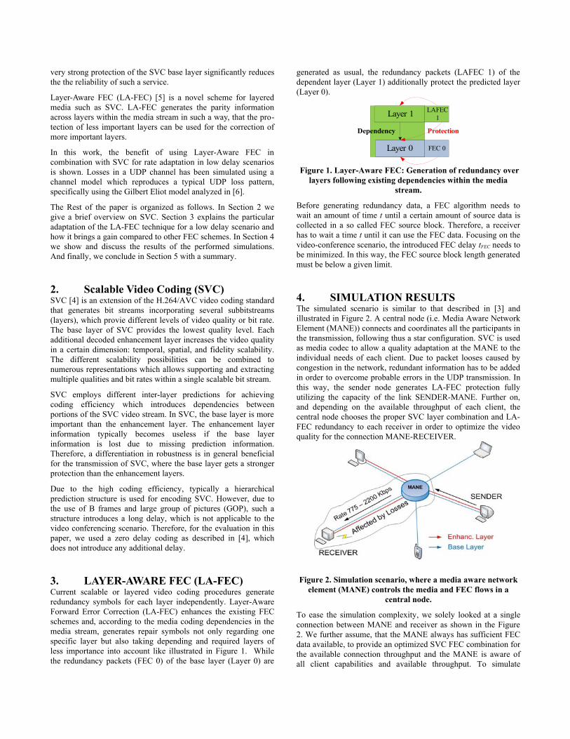
very strong protection of the SVC base layer significantly reducesthe the reliability of such a service.
Layer-Aware FEC (LA-FEC) [5] is a novel scheme for layeredmedia such as SVC. LA-FEC generates the parity informationacross layers within the media stream in such a way, that the pro-tection of less important layers can be used for the correction ofmore important layers.
In this work, the benefit of using Layer-Aware FEC incombination with SVC for rate adaptation in low delay scenariosis shown. Losses in a UDP channel has been simulated using achannel model which reproduces a typical UDP loss pattern,specifically using the Gilbert Eliot model analyzed in [6].
The Rest of the paper is organized as follows. In Section 2 wegive a brief overview on SVC. Section 3 explains the particularadaptation of the LA-FEC technique for a low delay scenario andhow it brings a gain compared to other FEC schemes. In Section 4we show and discuss the results of the performed simulations.And finally, we conclude in Section 5 with a summary.
2. Scalable Video Coding (SVC)SVC [4] is an extension of the H.264/AVC video coding standardthat generates bit streams incorporating several subbitstreams(layers), which provie different levels of video quality or bit rate.The base layer of SVC provides the lowest quality level. Eachadditional decoded enhancement layer increases the video qualityin a certain dimension: temporal, spatial, and fidelity scalability.The different scalability possibilities can be combined tonumerous representations which allows supporting and extractingmultiple qualities and bit rates within a single scalable bit stream.
SVC employs different inter-layer predictions for achievingcoding efficiency which introduces dependencies betweenportions of the SVC video stream. In SVC, the base layer is moreimportant than the enhancement layer. The enhancement layerinformation typically becomes useless if the base layerinformation is lost due to missing prediction information.Therefore, a differentiation in robustness is in general beneficialfor the transmission of SVC, where the base layer gets a strongerprotection than the enhancement layers.
Due to the high coding efficiency, typically a hierarchicalprediction structure is used for encoding SVC. However, due tothe use of B frames and large group of pictures (GOP), such astructure introduces a long delay, which is not applicable to thevideo conferencing scenario. Therefore, for the evaluation in thispaper, we used a zero delay coding as described in [4], whichdoes not introduce any additional delay.
3. LAYER-AWARE FEC (LA-FEC)Current scalable or layered video coding procedures generateredundancy symbols for each layer independently. Layer-AwareForward Error Correction (LA-FEC) enhances the existing FECschemes and, according to the media coding dependencies in themedia stream, generates repair symbols not only regarding onespecific layer but also taking depending and required layers ofless importance into account like illustrated in Figure 1. Whilethe redundancy packets (FEC 0) of the base layer (Layer 0) are
generated as usual, the redundancy packets (LAFEC 1) of thedependent layer (Layer 1) additionally protect the predicted layer(Layer 0).
Figure 1. Layer-Aware FEC: Generation of redundancy overlayers following existing dependencies within the media
stream.
Before generating redundancy data, a FEC algorithm needs towait an amount of time t until a certain amount of source data iscollected in a so called FEC source block. Therefore, a receiverhas to wait a time t until it can use the FEC data. Focusing on thevideo-conference scenario, the introduced FEC delay tFEC needs tobe minimized. In this way, the FEC source block length generatedmust be below a given limit.
4. SIMULATION RESULTSThe simulated scenario is similar to that described in [3] andillustrated in Figure 2. A central node (i.e. Media Aware NetworkElement (MANE)) connects and coordinates all the participants inthe transmission, following thus a star configuration. SVC is usedas media codec to allow a quality adaptation at the MANE to theindividual needs of each client. Due to packet looses caused bycongestion in the network, redundant information has to be addedin order to overcome probable errors in the UDP transmission. Inthis way, the sender node generates LA-FEC protection fullyutilizing the capacity of the link SENDER-MANE. Further on,and depending on the available throughput of each client, thecentral node chooses the proper SVC layer combination and LA-FEC redundancy to each receiver in order to optimize the videoquality for the connection MANE-RECEIVER.
Figure 2. Simulation scenario, where a media aware networkelement (MANE) controls the media and FEC flows in a
central node.
To ease the simulation complexity, we solely looked at a singleconnection between MANE and receiver as shown in the Figure2. We further assume, that the MANE always has sufficient FECdata available, to provide an optimized SVC FEC combination forthe available connection throughput and the MANE is aware ofall client capabilities and available throughput. To simulate
LAFEC1
FEC 0
Layer 1
Layer 0
ProtectionDependency

packet loss due to congestion we followed the loss ratesdescribed in [6]. Which, once introduced into the Gilbert ElliotModel mean an IP packet error rate of 22 % with a mean burstlength error average of 1.8 IP packets. We assumed the same errorprobabilities either for the base layer channel as well as for theenhancement layer channel.
A low delay SVC bit stream with two layers (QCIF + CIF) at aframe rate of 30 Hz had been encoded. The sequence, of about 30seconds, is a concatenation of the ITU-T test-sequencesCarphone, Foreman and Mother&Daughter using low delay SVCcoding (Scalable Baseline Profile, JSVM9.17). In case of framelosses, freeze frame error concealment is used, where the lastdecoded picture is just copied. In case only the enhancement layergets lost, the up scaled QVGA layer was used for PSNRcalculation. A summary of the encoding parameters for SVC andsimulcast can be found in Table 1.
Table 1. SVC media stream characteristics.
QualityVideo rate
[kbps] avg. PSNR
[dB]
SVC- baselayer
qCIF@30Hz 14330.86
(upscaled)
SVC- base +enhan.
CIF@30Hz 511 38.64
4.1 Effect of the Source Block LengthIn the first simulation results, we show the influence of the FECsource block length on unequal (UEP) and equal error protection(EEP) schemes using traditional FEC and LA-FEC. Differentsource block lengths has been selected for the simulated scenariowith a block length range going from 3 frames, which is equal to99 ms using a 30 frames per second video stream, to 150 framesor 5 s. The optimal code rate for base and enhancement layer hasbeen selected for each FEC scheme for a fixed service bitrate of800 kbps.
Figure 3. FEC Source Block Length from 1 to 150 frameswith an optimal code rate distribution for an 800 kbps service
bit rate.
Figure 3 shows the performance in terms of PSNR for eachprotection scheme using standard FEC and LA-FEC. It can be
seen, that a reduction of the source block length significantlyinfluences the protection capability of each simulated FECscheme. Moreover, it can be seen that the implementation of theLA-FEC protection brings a considerable gain in terms of PSNR,either when the layers are equal or unequal error protected.
For the following simulations, we have chosen a lengths of FECsource block of 3 frames, which introduces an delay by FEC of 99ms, which still leaves some free space for a video conferencingsystem.
4.2 Rate adaptation with Standard FECand LA-FECIn this section, the performance of the LA-FEC technique with theaforementioned scenario has been analyzed over a range ofservice bit rate available for the inspected link between MANETand RECEIVER going from about 775 Kbps to 2.2 Mbps. Themain target of the video conferencing application is to achieve aquasi error free base layer, which we assume is below an IPpacket error rate of 5%. The MANE starts sending theenhancement layer as soon as this constraint is fulfilled. The firstconsidered service bit rate value of 775 kbps corresponds with theminimum bit rate of 407 kbps needed to transmit the base layerwith an IP packet loss rate below 5% plus the requiredenhancement layer bit rate. The optimal code rate distributionamong the layers for each given service bit rate has been selected.The performance in terms of PSNR for standard FEC and LA-FEC is reported in Figure 4.
Figure 4. PSNR for LA-FEC and Standard FEC using anoptimal code rate distribution across layers for a given service
bitrate.
The plots start at 775 kbps which allows a transmission of theenhancement layer. From that point on, the enhancement layercode rate is reduced, so the protection of the layer increases ascan be seen in Figure 4. Using standard FEC, the code rate for thebase layer must be kept constant for all service bit rates to keepthe IP packet error rate below 5%. Using LA-FEC, the base layerprotection can be reduced, due to the increasing enhancementlayer protection also protects the base layer. This translates in aPSNR gain in the final reception of the bit stream. On thecontrary, in the traditional FEC simulations, since theenhancement layer protection does not influence the IP looses ofthe base layer after the FEC correction, the PSNR gain achievedis always lower until there is sufficient service bit rate (from
500 750 1000 1250 1500 1750 2000 2250 250030
31
32
33
34
35
36
37
38
39
Service Bit Rate [Kbps]
PS
NR
LA-FECStandard FEC
0.5 1 1.5 2 2.5 3 3.5 4 4.5
31
32
33
34
35
36
37
38
Length of TransportBlock [seconds]
PS
NR
Ave
rage
SVC , EEP , LA-FECSVC , EEP , Standard FECSVC , UEP , LA-FECSVC , UEP , Standard FEC

around 2200 Kbps bit rate on) available to protect both layers toget the maximum PSNR.
The results of the IP packet losses for base and enhancement layerafter the standard FEC or LA-FEC correction are depicted inFigure 5.
Figure 5. IP Packet Losses vs Service Bit Rate for base andenhancement layer packets.
Again, it can be seen that LA-FEC approach outperforms the FECscheme in terms of IP packet losses for the enhancement layerwhile keeping the base layer losses below 5%. For the currentanalyzed video stream, the gain is noticeable in a range of bitrates starting in 775 kbps to 1900 kbps for the enhancement layer.
The specific chosen code rate values for base and enhancementlayer for each service bit rate and FEC scheme are depicted inFigure 6.
Figure 6. Base and enhancement layer code rate for thedifferent FEC schemes at different service bit rates.
For the standard FEC simulations, the base layer code rate mustbe kept below a certain value of 0.45 to fulfill the IP packet lossconstraint. Therefore the protection for the enhancement layer can
be increased slow. For LA-FEC, the base layer code rate can besignificantly increased due to the additional protection from thedecreasing enhancement layer code rate. This allows to increasethe protection for the enhancement layer much faster whilemaintaining the base layer constraint as shown in Figure 6.
5. CONCLUSIONVideo conferencing solutions over a channel without QoS arevery sensitive to delay and packet losses. Multpoint videoconferencing systems additionally require the support of thedifferent connected device capabilities and throughput of thedifferent participants. This work presents a combination of SVCand layer-aware FEC (LA-FEC), which allows to support multiplevideo qualities and optimize protection for the available servicebit rate of each receiver while introducing low delay. Using LA-FEC allows to reduce the base layer protection while keeping itsIP packet loss rate below a certain level due to the additionalprotection from the enhancement layer. A central node (MANE)optimizes the available protection to maximize the experiencedvideo quality at the receiver. Simulation results for a singleconnection report a significant gain of using LA-FEC and SVCcompared to a standard FEC in terms of PSNR and IP packet lossrate. Future analysis will target a performance analysis of acomplete video conferencing system.
6. REFERENCES[1] ITU-T: ITU Recommendation G. 114, Series G:
Transmission Systems and Media, Digital Systems andNetworks, May, 2003.
[2] Yubo Tan, Yuxing Peng, Sikun Li, and Fujie Chen: AFEC:An Advanced FEC Algorithm for Video TransmissionControl over the Grid, Lecture Notes in Computer Science,Vol. 3252/2004, September 2004.
[3] Alexandros Eleftheriadis, M.. Reha Civanlar and OferShapiro: Multipoint videoconferencing with scalable videocoding. J. Zhejiang Univ. Sci. A, Vol. 7, No. 5, pp. 696-705,May 2006.
[4] Heiko Schwarz, Detlev Marpe and Thomas Wiegand:Overview of the Scalable Video Coding Extension of theH.264/AVC Standard. IEEE Transactions on circuits andsystems for video technology, Vol 17, No. 9, September2007.
[5] Cornelius Hellge, Thomas Schierl, and Thomas Wiegand:Mobile TV using scalable video coding and layer-awareForward Error Correction, IEEE International Conferenceon Multimedia and Expo (ICME'08), Hannover, Germany,June 23-26, 2008.
[6] Velibor Markovski, Fei Xue and Ljiljana Trajkovic :Simulation and Analysis of Packet Loss in User DatagramProtocol Transfers, The Journal of Supercomputing, Vol.20, No. 2, September 2001.
600 800 1000 1200 1400 1600 1800 2000 2200 24000
0.02
0.04
0.06
IP P
acke
t Los
s B
ase
Laye
r A
fter
FE
C
Service Bit Rate [Kbps]
600 800 1000 1200 1400 1600 1800 2000 2200 24000
0.1
0.2
0.3
IP P
acke
t Los
s E
nhan
cem
ent L
ayer
Afte
r F
EC
Base Layer IP Packet Loss: L-FEC ONBase Layer IP Packet Loss: L-FEC OFFEnhancement Layer IP Packet Loss: L-FEC ONEnhancement Layer IP Packet Loss: L-FEC OFF
500 1000 1500 2000 25000.2
0.3
0.4
0.5
0.6
0.7
0.8
0.9
1
Service Bit Rate [Kbps]
Cod
e R
ate
Enhancement Layer: LA-FECEnhancement Layer: Standard FECBase Layer: LA-FECBase Layer: Standard FEC

ii
B. Scientific paper submitted to
INFOCOM 2011

Adaptive Layer-Aware FEC for layered video transmission on error prone channels
Cornelius Hellge*,+, Nicolás Díez Risueño+, Thomas Schierl*,+, and Thomas Wiegand*,+
*Fraunhofer Institute for Telecommunications Heinrich Hertz Institute
Image Processing Department Einsteinufer 37
10587 Berlin, Germany
+Technische Universität Berlin Image Communication Group
Dep. of Telecommunication Systems Einsteinufer 17
10587 Berlin, Germany
{cornelius.hellge, nicolas.diez, thomas.schierl, thomas.wiegand}@hhi.fraunhofer.de
Abstract—Video data is very sensitive to transmission errors. The loss of coded video data on the channel may result in spatio-temporal error propagation in the video. This becomes more critical when layered media such as scalable video coding (SVC) or multiview video coding (MVC) is applied, which add additional inter-layer predictions. Transmission systems typically apply forward error correction (FEC) as mean to cope with transmission errors. FEC schemes, such as SVC Layer-Aware FEC (LA-FEC), take prediction structures within a layered media stream into account. The benefit of using LA-FEC in broadcast scenarios has already be shown in several publications, assuming a fixed service bit rate and code rate distribution across layers. In this paper, we show how SVC LA-FEC performs under variable throughput conditions. Simulations are based on a Gilbert-Elliot model derived from UDP connections over the open internet. The results report the optimal code rate distribution across the SVC layers for each FEC scheme under different throughput conditions and show the gain introduced by LA-FEC.
Keywords- Layer-Aware FEC, SVC, MVC
I. INTRODUCTION
Layered media codecs, such as scalable video coding (SVC) [1] or multi view coding (MVC) [2], offer a promising solution to video services for transmitting multiple service qualities within a single stream such as different resolutions, temporal or spatial qualities or providing 3D experience. Due to inter-layer prediction, layered media streams incorporate various inter-layer dependencies between the quality layers. Therefore, parts of the media stream are more important than the other. The loss of a quality layer affects all predicting layers. Thus, the transmission of layered media requires appropriate transmission scheme, providing a differentiation in robustness for the different quality layers.
Error control techniques such as Automatic Repeat reQuest (ARQ) or Forward Error Correction (FEC) can be used to cope with transmission errors. In this paper we focus on the use of FEC only. FEC mechanisms transmit additional repair data such that receivers can reconstruct the original information even if some transmission error occurs. Applying standard FEC (ST-FEC) to layered media, redundancy is generated separately for each quality layer. The traditional
FEC approach to achieve a more efficient delivery for multi layer media is to apply unequal error protection (UEP) [3] to the media stream, where the most important layers have a stronger FEC protection. Whereas FEC schemes, such as Layer-Aware FEC (LA-FEC), take prediction structures within a media stream into account by generating parity information across existing dependencies. The benefit of using LA-FEC in broadcast scenarios has already be shown in former publications, assuming a fixed service bit rate and code rate distribution across layers [4]. However, the optimal code rate distribution across layers depends on the available bit rate for protection, which requires an adaptive FEC solution for transmission systems as similarly shown in [5]. Applying FEC introduces an additional delay into the system, because of the receiver has to wait until all data of an FEC source block has been received before it can start correcting. Therefore, the allowed FEC source block length depends on the target application. E.g. video conferencing solutions as discussed in [6] require a very short delay [7] and the FEC source block length must be kept short.
In this paper, we show how SVC LA-FEC performs under variable throughput conditions. We further analyze the influence of the FEC source block length on the system performance. Moreover, we give a combinatorial analysis on performance of ST-FEC and LA-FEC schemes and proof them by further simulations. Simulations are based on a Gilbert-Elliot model derived from UDP connections over the open internet taken from [8]. Simulation results show the influence of the FEC source block length on the overall performance. Furthermore, the results report the optimal code rate distribution across the SVC layers for each FEC scheme under different throughput conditions and the gain introduced by LA-FEC in terms of required bit rate for an error free service.
The Rest of the paper is organized as follows. In Section II we give a brief overview on SVC. Section III explains how the LA-FEC technique for layered media works and how it brings a gain compared to other FEC schemes. In Section IV we present the simulation setup and give a combinatorial analysis of the selected scenario. In Section V we show and discuss the results of the performed simulations. And finally, we conclude in Section VI with a summary.

~ 2 ~
II. SCALABLE VIDEO CODING (SVC)
SVC [1] is an extension of the H.264/AVC video coding standard that generates bit streams incorporating several subbitstreams (layers), which provide different levels of video quality or bit rate. The base layer of SVC provides the lowest quality level. Each additional decoded enhancement layer increases the video quality in a certain dimension: temporal, spatial, and fidelity scalability. The different scalability possibilities can be combined to numerous representations which allows supporting and extracting multiple qualities and bit rates within a single scalable bit stream.
SVC employs different inter-layer predictions for achieving coding efficiency which introduces dependencies between portions of the SVC video stream. In SVC, the base layer is more important than the enhancement layers. The enhancement layer information typically becomes useless if the base layer information is lost due to missing prediction information. Therefore, a differentiation in robustness is in general beneficial for the transmission of SVC, where the base layer gets a stronger protection than the enhancement layers.
III. LAYER-AWARE FEC (LA-FEC)
In traditional FEC schemes for layered media transmission the redundancy is separately generated for each scalable layer. However, if the base layer cannot be corrected due to transmission errors, most of the enhancement layer information cannot be used due to missing reference pictures.
The main idea of SVC LA-FEC schemes, i.e. LA-FEC applied to SVC, is to generate the parity data of the enhancement layers following existing dependencies within the video stream [4]. Using LA-FEC, redundancy symbols of the less important SVC enhancement layers can jointly be used with symbols of more important layers (e.g., base layer) for error correction as shown in Figure 1. This effect comes without any increase in bit rate, and improves the reliability of the whole service. Fig. 2 depicts a simplified example with base and one enhancement layer, each with two source symbols and one parity symbol. Parity bits are generated by XOR combinations of source bits. Using ST-FEC scheme protects each layer separately. With LA-FEC, the generation of base layer parity symbol is the same as for the ST-FEC, but the parity symbol for the enhancement layer is generated across both layers. In the given example in Fig. 2, the standard FEC schemes allow correcting exactly one lost symbol in each layer (assuming an ideal code). Whereas the LA-FEC scheme allows the correction of up to two lost base layer symbols due to the additional connection of the parity symbol of the enhancement layer.
LA-FEC is a generic approach which can be applied to most FEC codes, such as e.g. LDPC or Raptor codes. A layer-aware Raptor implementation is used in this paper. Only small modifications on the Raptor encoding process are required to extend the symbol generation process while keeping its codewords systematic [4].
LAFEC1
FEC 0
Layer 1
Layer 0
ProtectionDependency
Figure 1. Generation of redundancy over layers following existing dependencies within the media stream
Figure 2. Additional protection to more important layers by generating redundancy over source blocks (SB) across layers
Using an ideal and standard FEC, a particular layer l can be decoded if the number of received symbols rl is equal or larger than the number of source symbols kl of the layer following the condition Cond A in equation (1).
Cond A: rl ≥ kl (1)
With LA-FEC, the enhancement layer l=1 can be used for
joint decoding which increases the decoding probability of the base layer. Thereby, the decoding probability for the base layer increases and base layer can be decoded if the condition Cond B in equation (2) is fulfilled.
Cond B: Cond A (r0+(r1 - k1) ≥ k0) (2)
On the other side, the decoding probability of the
enhancement layer is decreased due to the additional dependencies within the FEC. The enhancement layer can be corrected if the base layer can be corrected. Therefore, the enhancement layer can be decoded if condition Cond C in equation (3) is true.
Cond C: Cond B (r1 ≥ k1) (3)
However, due to the enhancement layer data is useless in
case of lost base layer, there is no significant impact on the perceived video quality when applying LA-FEC.
IV. SIMULATION SETUP
A. Scenario
The simulated scenario is illustrated in Fig. 3. A connection between a SENDER and RECEIVER is simulated. The connection is affected by losses simulated by a Gilbert Elliot Model (GE) and the available bit rate is varied from 0-1075 kbps. The SENDER provides a single scalable stream

~ 3 ~
with two resolutions, qCIF and CIF. There is no means for any media coding or transcoding available at the SENDER. Moreover, the SENDER is aware of the available throughput and loss rates based on feedback received from the RECEIVER. The only way for the SENDER to adapt to the given channel conditions is to apply FEC to each layer. The further sections explaines, how the video coding stream, the packet losses, and the FEC redundancy are simulated.
Figure 3. Simulation scenario. The sender transmits a SVC stream over channel affected by packet losses
B. Video Coding and transmission scheduling
To reduce the overall system delay, a low delay SVC bit stream with two layers, base (qCIF) and enhancement (CIF), at a frame rate of 30 Hz has been encoded. The sequence, of about 30 seconds, is a concatenation of the ITU-T test-sequences Carphone, Foreman and Mother&Daughter using low delay SVC coding (Scalable Baseline Profile, JSVM9.17). In case of frame losses, freeze frame error concealment is used, where the last decoded picture is just copied. In case only the enhancement layer gets lost, the up scaled qCIF layer was used for PSNR calculation. A summary of the encoding parameters for SVC can be found in Table I.
TABLE I. SVC MEDIA STREAM CHARACTERISTICS
Quality
Video Rate
[kbps]
Avg. PSNR [dB]
SVC – base
layer
qCIF@30Hz 164 31.87
(upscaled)
SVC – base + enhancement
CIF@30Hz 544 38.64
Depending on the available bit rate, the SENDER is able to send the base layer, the enhancement layer, the FEC protection of the base layer or the- LA-FEC protection of the enhancement layer. The SENDER relies on the following transmission schedule: first the base layer is transmitted and base layer FEC protection is increased until the IP packet error rate of the base layer is below 1% and base layer is received quasi error free. At higher bitrates, the enhancement layer is transmitted while keeping the base layer in error free state. And finally the FEC/LA-FEC protection of the enhancement layer is
increased until IP packet error rate of enhancement layer falls below 1%.
C. Channel simulation
To simulate packet loss due to congestion we assumed the loss rates probabilities described in [8]. Which, once introduced into the Gilbert Elliot Model mean an IP packet error rate of 22 % with a mean burst length error average of 1.8 IP packets. In the performed simulations the generated IP packets are equal size to the MTU size, which means 1400 bytes. Occasionally some IP packets result with a smaller size due to fragmentation issues. The Gilbert Elliot diagram is based on a two state Markow-model as shown in Fig. 4. State 0 represents the state of successful arrival of the packet, while state 1 represents the state of packet lost. The transition probability p10 from state 1 to state 0, the transition probability p01 from state 0 to state 1 as well as the IP packet error rate and the average burst length are summarized in Table II. For deep detailed calculations of the mentioned data resort to [8]. The simulations have been carried out increasing the bit rate available of the channel and choosing the optimal code rates for each point. Starting at bit rate 0 kbps, we increase the throughput of the link until the enhancement layer reaches an IP packet loss rate of 1%, which corresponds with a bit rate value of 1075 kbps.
TABLE II. PARAMETERS OF GILBERT ELLIOT CHANNEL MODEL
State Transition Channel Parameters
p10
p01 IP packet error
rate Average burst
length
0.5479
0.0986 22% 1.8 IP packets
Figure 4. State diagram of the Gilbert Elliot model used for packet loss simulation
D. FEC redundancy
Due to packet looses caused by congestion in the networks, redundant information has to be added in order to overcome probable errors in the UDP transmission. In the simulated link, the SENDER node generates ST-FEC or LA-FEC protection based on Raptor FEC fully utilizing the available capacity of the link.
Regarding the optimization of the code rates, is important to highlight that, when transmitting more than one layer, there are many code rate combinations of base and enhancement layer which satisfy each bit rate value. In the simulations performed, the code rate combination chosen has always been the one which leads in lowest IP packet lost rate for the enhancement layer (further on more details about when enhancement layer starts being transmitted will be explained) while keeping the base layer IP packet losses below 1%.

~ 4 ~
E. Combinatorical Analysis
In this section we analyze the performance of LA-FEC in comparison with ST-FEC by a combinatorial analysis based on the conditions (1), (2), and (3) in Section III.
The conducted analysis is based on a toy example, where two layers, layer 0 and layer 1, are sent over an erroneous channel. Due to prediction within the media codec, layer 1 depends on layer 0. Each layer l consists of a certain amount of source symbols kl and a number of parity symbols pl. The symbols of all layers are sent over an erroneous channel and transmission errors result in lost symbols. We assume a channel where each distribution across layers of a number of received symbols rl, referred to as loss constellation, has the same probability. We assume an ideal FEC code, where source symbols can be corrected as soon as k symbols have been received. The exemplary settings in Fig. 5 are derived from the bit rate ratio between the two layers from the SVC encodings given in Section IV.B. Therefore, the number source symbols kl per layer l is kept constant at k0=2 and k1=6 while the number of parity bits p=p0+p1 is increased. For each parity bit distribution across layers we calculate the average decoding probability for all possible reception conditions of a given number of lost symbols l=n-r. Fig. 5 depicts an exemplary setting with, k0=2, k1=6, p0=4, p1=0, r0=2 and r1=4 and n=12.
Figure 5. One exemplary loss constellation for n=n0+n1 =12 transmitted and r=r0+r1=6 received symbols
For each loss constellation we calculate the decoding probability for each layer based on the conditions from Section III. The overall number of sent packets n is increased while keeping the number of source symbols k0 and k1 constant. The decoding probability of each code rate distribution for each layer is calculated at an received packets value of 70%, which corresponds to the selected average losses of 22% of the selected GE channel (see Section IV.C). Based on these probability calculations, we selected the highest base layer code rate giving a base layer decoding probability of 90%. Note that the highest base layer code rate fulfilling the decoding constraint allows to maximize the protection of the enhancement layer. The calculated optimal code rates for base and enhancement layer for ST-FEC and LA-FEC scheme are shown in Figure 6. The curves show the influence of the LA-FEC on the base layer. While for ST-FEC, the base layer code rate has to be kept constant to keep the target base layer decoding probability of 90%, for LA-FEC, the protection can be reduced. The released bit rate can be used for a higher protection of the enhancement layer which increases the overall performance.
0,40
0,50
0,60
0,70
0,80
0,90
1,00
1 2 3 4 5
Code rate
Number of parity symbols p = p0+p1
LA‐FEC Base layer
LA‐FEC Enh. layer
ST‐FEC Base layer
ST‐FEC Enh. layer
Figure 6. Optimal code rate distribution at symbol loss rate of 70% and a
minimum base layer decoding probability of 90%
0 2 4 6 8 10 12 14 16 1826
28
30
32
34
36
38
40
FEC Source Block Length [seconds]
PS
NR
Ave
rage
[dB
]
ST-FEC / EEPST-FEC / UEPLA-FEC / EEPLA-FEC / UEP
Figure 7. FEC Source Block Length from 0.033 ms to 17 sec. with an optimal code rate distribution for an 800 Kbps service bitrate using standard FEC (ST-
FEC) and Layer-Aware FEC (LA-FEC) with equal and unequal error protection (EEP and UEP)

~ 5 ~
V. SIMULATION RESULTS
A. Influence of the FEC source block length
Applying FEC introduces some delay due to the receiver has to wait until all data of a FEC source block has been received before it can start decoding. Therefore, the applicable length of an FEC source block depends on the target application. In the first simulation results, we show the influence of the FEC source block length on unequal (UEP) and equal error protection (EEP) schemes using traditional FEC and LA-FEC. Both, base and enhancement layer, are transmitted with the optimal code rate protection depending on the FEC source block length for each point. Different FEC source block lengths have been selected for the simulated scenario with a block length range going from 3 frames, which is equal to 99 ms using a 30 frames per second video stream, to 515 frames or 17 s. The optimal code rate for base and enhancement layer has been selected for each FEC scheme for a fixed service bit rate of 800 kbps.
Fig. 7 shows the performance in terms of PSNR under different FEC source block length for each protection scheme using ST-FEC and LA-FEC. It can be seen, that a reduction of the source block length significantly influences the protection capability of each simulated FEC scheme. Moreover, it can be seen that the implementation of the LA-FEC protection brings a considerable gain in terms of PSNR, either when the layers are equal or unequal error protected. For the following simulations, we have chosen a length of FEC source block of 16 frames, which introduces a delay by FEC of 0.528 s. Different FEC source block lengths may be chosen when adapting to different delay-required systems. E.g. a FEC source block length between 0 and 150 ms might be chosen for Video Conferencing applications. Moreover, FEC sizes of 1 to 2 sec.
would be suitable for mobile TV systems and so on.
B. Optimal code rate distribution for ST-FEC and LA-FEC under variable throughput condition
In this section, the performance of the LA-FEC technique in the aforementioned scenario has been analyzed over a range of service bit rate available for the inspected link between SENDER and RECEIVER going from 0 kbps to 1075 kbps. Due to the main target of most of the video applications, a quasi error free base layer is usually desired at reception. In this regard, a value of 1% IP packet loss rate is the threshold we assumed as error free base layer.
The performed simulations show the behavior of the base and enhancement layer depending on the bit rate available. Specifically, we analyze and plot for each layer the performance of the code rates applied (Fig. 8), the IP packet loss rate experienced in the transmission (Fig. 9) and the PSNR obtained in reception after the final decoding and correction steps (Fig. 10). Due to the higher importance of the base layer within the SVC stream as explained before, the base layer is transmitted in first term. Moreover, an IP packet loss rate of 1% in the base layer is the target to reach before any attempt of transmitting the enhancement layer. When sufficient bit rate, the enhancement layer will be transmitted until the same packet loss rate is achieved.
Regarding Fig. 8 and Fig. 9:
Area A: Between 0 and 164 Kbps, there is not enough bit rate available to transmit the base layer, no transmission is possible.
Area B: When a bit rate of 164 Kbps is available, the transmission of the base layer can be started. Firstly, the base layer is transmitted unprotected due to no
100 200 300 400 500 600 700 800 900 1000 11000.4
0.5
0.6
0.7
0.8
0.9
1
Service Bit Rate [Kbps]
Cod
e R
ate
ST-FEC Base LayerST-FEC Enhancement LayerLA-FEC Base LayerLA-FEC Enhancement Layer
Figure 8. Code rates vs. Bit Rate available for Standard FEC (ST-FEC) and Layer-Aware FEC (LA-FEC)
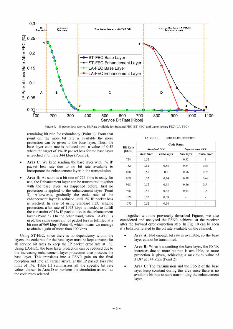
~ 6 ~
remaining bit rate for redundancy (Point 1). From that point on, the more bit rate is available the more protection can be given to the base layer. Thus, the base layer code rate is reduced until a value of 0.52 where the target of 1% IP packet loss for the base layer is reached at bit rate 344 kbps (Point 2).
Area C: We keep sending the base layer with 1% IP packet loss rate due to no bit rate available to incorporate the enhancement layer in the transmission.
Area D: As soon as a bit rate of 724 kbps is ready for use, the Enhancement layer can be transmitted together with the base layer. As happened before, first no protection is applied to the enhancement layer (Point 3). Afterwards, gradually the code rate of the enhancement layer is reduced until 1% IP packet loss is reached. In case of using Standard FEC scheme protection, a bit rate of 1073 kbps is needed to fulfill the constraint of 1% IP packet loss in the enhancement layer (Point 5). On the other hand, when LA-FEC is used, the same constraint of packet loss is fulfilled at a bit rate of 969 kbps (Point 4), which means we manage to obtain a gain of more than 100 kbps.
Using ST-FEC, since there is no dependency within the layers, the code rate for the base layer must be kept constant for all service bit rates to keep the IP packet error rate at 1%. Using LA-FEC, the base layer protection can be reduced due to the increasing enhancement layer protection also protects the base layer. This translates into a PSNR gain on the final reception and into an earlier arrival at the IP packet loss rate limit of 1%. Table III summarizes all the specific bit rate values chosen in Area D to perform the simulation as well as the code rates selected.
TABLE III. CODE RATES SELECTED
Bit Rate [kbps]
Code Rates
Standard FEC Layer-Aware FEC
Base layer Enha. layer Base layer Enha. layer
724 0,52 1 0,52 1
782 0,52 0,88 0,54 0,86
828 0,52 0,8 0,56 0,76
869 0,52 0,74 0,58 0,68
918 0,52 0,68 0,86 0,54
976 0,52 0,62 0,94 0,5
1021 0,52 0,58 - -
1073 0,52 0,54 - -
Together with the previously described Figures, we also considered and analyzed the PSNR achieved at the receiver after the forward error correction step. In Fig. 10 can be seen it´s behavior related to the bit rate available on the channel:
Area A: Not enough bit rate is available, so the base layer cannot be transmitted.
Area B: When transmitting the base layer, the PSNR increases due to more bit rate is available, so more protection is given, achieving a maximum value of 31.87 at 344 kbps (Point 2).
Area C: The transmission and the PSNR of the base layer keep constant during this area since there is no available bit rate to start transmitting the enhancement layer.
100 200 300 400 500 600 700 800 900 1000 11000
0.01
0.05
0.1
0.15
0.2
0.25
0.3
Service Bit Rate [Kbps]
IP P
acke
t Lo
ss R
ate
Afte
r F
EC
[%]
ST-FEC Base LayerST-FEC Enhancement LayerLA-FEC Base LayerLA-FEC Enhancement Layer
Figure 9. IP packet loss rate vs. Bit Rate available for Standard FEC (ST-FEC) and Layer-Aware FEC (LA-FEC)

~ 7 ~
Area D: When enhancement layer is transmitted along with the base layer, the difference between the two FEC protection schemes can be seen. While the ST-FEC simulation is reaching the highest PSNR at 1073 kbps (Point 5), the LA-FEC scheme is doing so at 969 kbps (Point 4). Once more, LA-FEC outperforms the ST- FEC technique in terms of PSNR. The gain is especially noticeable from 920 kbps on, where a difference between the two schemes of more than 1.5 dB is obtained at some points.
VI. CONCLUSION
Video transmission solutions over a channel without QoS are very sensitive to packet losses. This becomes more critical when layered media such as SVC or MVC is applied. To cope with these channel errors, FEC protection techniques can be used. This work analyzes, how SVC and Layer-Aware FEC (LA-FEC) performs under varying throughput conditions. A combinatorial analysis of the selected scenario is given. Simulation results for a single connection report a significant gain of using LA-FEC and SVC compared to a standard FEC in terms of bit rate, PSNR and IP packet loss rate. Future works will target a performance analysis of more complex video scenarios.
REFERENCES [1] H. Schwarz, D. Marpe and T. Wiegand, “Overview of the scalable video
coding extension of the H.264/AVC standard,” IEEE Transactions on circuits and systems for video technology, Vol 17, No. 9, September 2007.
[2] P. Merkle, Y. Morvan, A. Smolic, D. Farin, K. Müller, P.H.N. de With, and T. Wiegand, "The effects of multiview depth video compression on multiview rendering,"Signal Processing: Image Communication - special issue on advances in three-dimensional television and video, vol. 24, issues 1-2, pp. 73-88, January 2009.
[3] A. Albanese, J. Blomer, J. Edmonds, M. Luby and M. Sudan, ”Priority encoding transmission,”IEEE Trans. on Information Theory, 42(6):1737-1744, 1996.
[4] C. Hellge, T. Schierl, and T. Wiegand, “Mobile TV using scalable video coding and layer-aware forward error correction,” IEEE International Conference on Multimedia and Expo (ICME'08), Hannover, Germany, June 23-26, 2008.
[5] Y. Tan, Y. Peng, S. Li, and F. Chen, “AFEC: An advanced FEC algorithm for video transmission control over the grid,” Lecture Notes in Computer Science, Vol. 3252/2004, September 2004.
[6] A. Eleftheriadis, M. Reha Civanlar and O. Shapiro, “multipoint videoconferencing with scalable video coding,” J. Zhejiang Univ. Sci. A, Vol. 7, No. 5, pp. 696-705, May 2006.
[7] ITU-T: ITU Recommendation G. 114, Series G, “Transmission systems and media,” Digital Systems and Networks, May, 2003.
[8] V. Markovski, F. Xue, and L. Trajkovic, “Simulation and analysis of packet loss in user datagram protocol transfers,” The Journal of Supercomputing, Vol. 20, No. 2, September 2001.
100 200 300 400 500 600 700 800 900 1000 110024
26
28
30
32
34
36
38
40
Service Bit Rate [Kbps]
PS
NR
[dB
]
ST-FECLA-FEC
Figure 10. PSNR vs. Bit Rate available for Standard FEC (ST-FEC) and Layer-Aware FEC (LA-FEC)

i
PRESUPUESTO
1) Ejecución Material
- Compra de ordenador personal (Software incluido) .................................... 1.500 €
- Alquiler de impresora láser durante 18 meses ................................................. 100 €
- Material de oficina ............................................................................................. 100 €
- Total de ejecución material ............................................................................ 1.700 €
2) Gastos generales
- 16 % sobre Ejecución Material .......................................................................... 272 €
3) Beneficio Industrial
- 6 % sobre Ejecución Material ............................................................................ 102 €
4) Honorarios Proyecto
- 1440 horas a 10 € / hora ................................................................................ 14400 €
5) Material fungible
- Gastos de impresión ........................................................................................... 50 €
- Encuadernación ................................................................................................. 200 €

ii
6) Subtotal del presupuesto
- Subtotal Presupuesto .................................................................................... 16622 €
7) I.V.A. aplicable
- 16% Subtotal Presupuesto ......................................................................... 2659 €
8) Total presupuesto
- Total Presupuesto ...................................................................................... 19281 €
Madrid, Junio de 2011
El Ingeniero Jefe de Proyecto
Fdo.: Nicolás Díez Risueño
Ingeniero Superior de Telecomunicación

iii

iv
PLIEGO DE CONDICIONES
Este documento contiene las condiciones legales que guiarán la realización, en este
proyecto, de Transmisión de video codificado en capas usando Media Aware Forward
Error Correction. En lo que sigue, se supondrá que el proyecto ha sido encargado por una
empresa cliente a una empresa consultora con la finalidad de realizar dicho sistema. Dicha
empresa ha debido desarrollar una línea de investigación con objeto de elaborar el proyecto.
Esta línea de investigación, junto con el posterior desarrollo de los programas está amparada
por las condiciones particulares del siguiente pliego.
Supuesto que la utilización industrial de los métodos recogidos en el presente
proyecto ha sido decidida por parte de la empresa cliente o de otras, la obra a realizar se
regulará por las siguientes:
Condiciones generales
1. La modalidad de contratación será el concurso. La adjudicación se hará, por tanto,
a la proposición más favorable sin atender exclusivamente al valor económico, dependiendo
de las mayores garantías ofrecidas. La empresa que somete el proyecto a concurso se
reserva el derecho a declararlo desierto.
2. El montaje y mecanización completa de los equipos que intervengan será realizado
totalmente por la empresa licitadora.
3. En la oferta, se hará constar el precio total por el que se compromete a realizar la
obra y el tanto por ciento de baja que supone este precio en relación con un importe límite
si este se hubiera fijado.
4. La obra se realizará bajo la dirección técnica de un Ingeniero Superior de
Telecomunicación, auxiliado por el número de Ingenieros Técnicos y Programadores que se
estime preciso para el desarrollo de la misma.
5. Aparte del Ingeniero Director, el contratista tendrá derecho a contratar al resto del
personal, pudiendo ceder esta prerrogativa a favor del Ingeniero Director, quien no estará
obligado a aceptarla.
6. El contratista tiene derecho a sacar copias a su costa de los planos, pliego de
condiciones y presupuestos. El Ingeniero autor del proyecto autorizará con su firma las
copias solicitadas por el contratista después de confrontarlas.

v
7. Se abonará al contratista la obra que realmente ejecute con sujeción al proyecto
que sirvió de base para la contratación, a las modificaciones autorizadas por la superioridad
o a las órdenes que con arreglo a sus facultades le hayan comunicado por escrito al
Ingeniero Director de obras siempre que dicha obra se haya ajustado a los preceptos de los
pliegos de condiciones, con arreglo a los cuales, se harán las modificaciones y la valoración
de las diversas unidades sin que el importe total pueda exceder de los presupuestos
aprobados. Por consiguiente, el número de unidades que se consignan en el proyecto o en el
presupuesto, no podrá servirle de fundamento para entablar reclamaciones de ninguna
clase, salvo en los casos de rescisión.
8. Tanto en las certificaciones de obras como en la liquidación final, se abonarán los
trabajos realizados por el contratista a los precios de ejecución material que figuran en el
presupuesto para cada unidad de la obra.
9. Si excepcionalmente se hubiera ejecutado algún trabajo que no se ajustase a las
condiciones de la contrata pero que sin embargo es admisible a juicio del Ingeniero Director
de obras, se dará conocimiento a la Dirección, proponiendo a la vez la rebaja de precios que
el Ingeniero estime justa y si la Dirección resolviera aceptar la obra, quedará el contratista
obligado a conformarse con la rebaja acordada.
10. Cuando se juzgue necesario emplear materiales o ejecutar obras que no figuren
en el presupuesto de la contrata, se evaluará su importe a los precios asignados a otras
obras o materiales análogos si los hubiere y cuando no, se discutirán entre el Ingeniero
Director y el contratista, sometiéndolos a la aprobación de la Dirección. Los nuevos precios
convenidos por uno u otro procedimiento, se sujetarán siempre al establecido en el punto
anterior.
11. Cuando el contratista, con autorización del Ingeniero Director de obras, emplee
materiales de calidad más elevada o de mayores dimensiones de lo estipulado en el
proyecto, o sustituya una clase de fabricación por otra que tenga asignado mayor precio o
ejecute con mayores dimensiones cualquier otra parte de las obras, o en general, introduzca
en ellas cualquier modificación que sea beneficiosa a juicio del Ingeniero Director de obras,
no tendrá derecho sin embargo, sino a lo que le correspondería si hubiera realizado la obra
con estricta sujeción a lo proyectado y contratado.
12. Las cantidades calculadas para obras accesorias, aunque figuren por partida
alzada en el presupuesto final (general), no serán abonadas sino a los precios de la contrata,
según las condiciones de la misma y los proyectos particulares que para ellas se formen, o en
su defecto, por lo que resulte de su medición final.

vi
13. El contratista queda obligado a abonar al Ingeniero autor del proyecto y director
de obras así como a los Ingenieros Técnicos, el importe de sus respectivos honorarios
facultativos por formación del proyecto, dirección técnica y administración en su caso, con
arreglo a las tarifas y honorarios vigentes.
14. Concluida la ejecución de la obra, será reconocida por el Ingeniero Director que a
tal efecto designe la empresa.
15. La garantía definitiva será del 4% del presupuesto y la provisional del 2%.
16. La forma de pago será por certificaciones mensuales de la obra ejecutada, de
acuerdo con los precios del presupuesto, deducida la baja si la hubiera.
17. La fecha de comienzo de las obras será a partir de los 15 días naturales del
replanteo oficial de las mismas y la definitiva, al año de haber ejecutado la provisional,
procediéndose si no existe reclamación alguna, a la reclamación de la fianza.
18. Si el contratista al efectuar el replanteo, observase algún error en el proyecto,
deberá comunicarlo en el plazo de quince días al Ingeniero Director de obras, pues
transcurrido ese plazo será responsable de la exactitud del proyecto.
19. El contratista está obligado a designar una persona responsable que se entenderá
con el Ingeniero Director de obras, o con el delegado que éste designe, para todo
relacionado con ella. Al ser el Ingeniero Director de obras el que interpreta el proyecto, el
contratista deberá consultarle cualquier duda que surja en su realización.
20. Durante la realización de la obra, se girarán visitas de inspección por personal
facultativo de la empresa cliente, para hacer las comprobaciones que se crean oportunas. Es
obligación del contratista, la conservación de la obra ya ejecutada hasta la recepción de la
misma, por lo que el deterioro parcial o total de ella, aunque sea por agentes atmosféricos u
otras causas, deberá ser reparado o reconstruido por su cuenta.
21. El contratista, deberá realizar la obra en el plazo mencionado a partir de la fecha
del contrato, incurriendo en multa, por retraso de la ejecución siempre que éste no sea
debido a causas de fuerza mayor. A la terminación de la obra, se hará una recepción
provisional previo reconocimiento y examen por la dirección técnica, el depositario de
efectos, el interventor y el jefe de servicio o un representante, estampando su conformidad
el contratista.
22. Hecha la recepción provisional, se certificará al contratista el resto de la obra,
reservándose la administración el importe de los gastos de conservación de la misma hasta

vii
su recepción definitiva y la fianza durante el tiempo señalado como plazo de garantía. La
recepción definitiva se hará en las mismas condiciones que la provisional, extendiéndose el
acta correspondiente. El Director Técnico propondrá a la Junta Económica la devolución de
la fianza al contratista de acuerdo con las condiciones económicas legales establecidas.
23. Las tarifas para la determinación de honorarios, reguladas por orden de la
Presidencia del Gobierno el 19 de Octubre de 1961, se aplicarán sobre el denominado en la
actualidad “Presupuesto de Ejecución de Contrata” y anteriormente llamado ”Presupuesto
de Ejecución Material” que hoy designa otro concepto.
Condiciones particulares
La empresa consultora, que ha desarrollado el presente proyecto, lo entregará a la
empresa cliente bajo las condiciones generales ya formuladas, debiendo añadirse las
siguientes condiciones particulares:
1. La propiedad intelectual de los procesos descritos y analizados en el presente
trabajo, pertenece por entero a la empresa consultora representada por el Ingeniero
Director del Proyecto.
2. La empresa consultora se reserva el derecho a la utilización total o parcial de los
resultados de la investigación realizada para desarrollar el siguiente proyecto, bien para su
publicación o bien para su uso en trabajos o proyectos posteriores, para la misma empresa
cliente o para otra.
3. Cualquier tipo de reproducción aparte de las reseñadas en las condiciones
generales, bien sea para uso particular de la empresa cliente, o para cualquier otra
aplicación, contará con autorización expresa y por escrito del Ingeniero Director del
Proyecto, que actuará en representación de la empresa consultora.
4. En la autorización se ha de hacer constar la aplicación a que se destinan sus
reproducciones así como su cantidad.
5. En todas las reproducciones se indicará su procedencia, explicitando el nombre del
proyecto, nombre del Ingeniero Director y de la empresa consultora.
6. Si el proyecto pasa la etapa de desarrollo, cualquier modificación que se realice
sobre él, deberá ser notificada al Ingeniero Director del Proyecto y a criterio de éste, la
empresa consultora decidirá aceptar o no la modificación propuesta.

viii
7. Si la modificación se acepta, la empresa consultora se hará responsable al mismo
nivel que el proyecto inicial del que resulta el añadirla.
8. Si la modificación no es aceptada, por el contrario, la empresa consultora declinará
toda responsabilidad que se derive de la aplicación o influencia de la misma.
9. Si la empresa cliente decide desarrollar industrialmente uno o varios productos en
los que resulte parcial o totalmente aplicable el estudio de este proyecto, deberá
comunicarlo a la empresa consultora.
10. La empresa consultora no se responsabiliza de los efectos laterales que se puedan
producir en el momento en que se utilice la herramienta objeto del presente proyecto para
la realización de otras aplicaciones.
11. La empresa consultora tendrá prioridad respecto a otras en la elaboración de los
proyectos auxiliares que fuese necesario desarrollar para dicha aplicación industrial, siempre
que no haga explícita renuncia a este hecho. En este caso, deberá autorizar expresamente
los proyectos presentados por otros.
12. El Ingeniero Director del presente proyecto, será el responsable de la dirección de
la aplicación industrial siempre que la empresa consultora lo estime oportuno. En caso
contrario, la persona designada deberá contar con la


