Prudence Demands Conservatism May 2012 Michael T. Kirschenheiter and Ram Ramakrishnan 12 1 College of Business Administration, University of Illinois at Chicago, 601 South Morgan Street, (MC 006), Chicago, Illinois, rooms 2309 and 2302, respectively. 2 We would like to thank Judson Caskey, Mingcherng Deng, Frank Gigler, Bjorn N. Jorgensen, Chan- dra Kanodia, Carolyn Levine, Ivan Marinovic, Jeroen Suijs, seminar participants at Universities of Illinois at Chicago, University of Minnesota and Colorado at Boulder, the 2009 Financial Economics and Accounting Conference at Rutger University for helpful comments on earlier drafts. 1
Transcript
Prudence Demands Conservatism
May 2012
Michael T. Kirschenheiter and Ram Ramakrishnan1 2
1College of Business Administration, University of Illinois at Chicago, 601 South Morgan Street,(MC 006), Chicago, Illinois, rooms 2309 and 2302, respectively.
2We would like to thank Judson Caskey, Mingcherng Deng, Frank Gigler, Bjorn N. Jorgensen, Chan-dra Kanodia, Carolyn Levine, Ivan Marinovic, Jeroen Suijs, seminar participants at Universities ofIllinois at Chicago, University of Minnesota and Colorado at Boulder, the 2009 Financial Economicsand Accounting Conference at Rutger University for helpful comments on earlier drafts.
1
Prudence Demands ConservatismAbstract
We define accounting systems as conditionally conservative (or liberal) if they pro-duce finer information at lower (or higher) expected earning levels. We study the pref-erence for differing levels of conservatism among decision-maker (DM)’s with varyingrisk aversion and prudence. Similar to risk aversion, prudence is a metric based onDM’s indirect utility; prudent DM’s save more as income becomes riskier. In a modelof precautionary savings with information, we show that prudent DM’s (those withpositive prudence measures) prefer more conservative accounting systems and thatimprudent DM’s (those with negative prudence measures) prefer liberal accountingsystems. We also show that conservative accounting may be preferred to a perfect(i.e., perfectly fine) information system if the signals are costly. We provide casesdemonstrating the generality of our results, including examples where conservatismis preferred with increasing, constant and decreasing risk aversion.
2
1 Introduction
Conditional conservatism has been described as responding to news or informationin a manner that results in reporting lower income, but deferring the recognition ofhigher income; in the extreme case, this has been interpreted to mean ‘anticipate noprofits but anticipate all losses.’3 While conditionally conservative accounting meth-ods are prevalent in current accounting standards, standard setters seem opposed todesigning standards to be explicitly conservative.4 For example, in rerewriting chap-ter 3 of Statement of Financial Accounting Concepts No. 8, ‘Qualitative Character-istics of Useful Financial Information ’, the Financial Accounting Standards Boardexplicitly exclude conservatism as a useful characteristic of financial information,judging it to be ‘inconsistent with neutrality ’and stating that ‘an admonition to beprudent is likely to lead to a bias.’5 With due respect to this viewpoint, we believe analternative perspective where conservatism does not lead to bias is possible.
Conditional conservatism has generated considerable interest, which in turn hasresulted in a considerable amount of research on the topic. Despite this effort, thereremains a dearth of simple formal explanations for the existence and preference forconditional conservative accounting methods. We know conservative methods existand, despite the perspective of some researchers and standard setters, we feel prac-tical accountants like or prefer these methods, but we do not have a simple, formalmodel to explain why. Our objective is to develop such a model.
We define information systems as being conditionally conservative if they pro-duce finer information at lower earnings levels and, analogously, we define informa-tion systems as being conditionally liberal if they produce finer information at higherearnings levels. In doing so, we provide an alternative perspective where conser-vatism does not necessarily lead to bias; rather conservatism leads to differentialtiming in recognizing good and bad news, but in an unbiased manner. We measureprudence as the sensitivity of expected utility maximizing decision makers (DM’s) tothe variability of a decision variable to risk. Similar to the Arrow - Pratt measure ofrisk aversion, the measure of prudence depends on a DM’s basic preference orderingas quantified by a DM’s indirect utility funtion. More specifically, prudence is the
3See Watts (2003a).4See section 3.4 below for more detailed discussion of the conditionally conservative accounting
methods prevalent in current US GAAP.5See FASB (2010), paragraphs BC3.27 and BC3.28, respectively. Also, in these paragraphs, FASB
seems to conflate prudence and conservatism, interpreting them as interchangeable concepts. In con-trast, we distinguish between conservatism, which is a characteristic of the accounting system, andprudence, which describes a DM’s preferences.
3
negative of the ratio of the second and third derivatives of the utility function andmeasures the sensitivity of a DM’s savings decision to risk; prudent DM’s save moreas income becomes riskier while imprudent DM’s save less as income becomes riskier.Using this definition of conservatism and this measure of prudence, we derive thefollowing results.
First, in a model of conservatism with precautionary savings, we show that pru-dent DM’s (those with positive prudence measures) prefer conservative accountingsystems to liberal accounting systems. Second, we show that DM’s with prudenceneutral preferences (prudence measure equal to zero) are indifferent to the conserva-tive or liberal reporting systems. Third, we show that imprudent DM’s (those withnegative prudence measures) prefer liberal accounting systems. Fourth, we showthat conservatism is preferred by prudent DM’s over an accounting system that fullyrecognizes income based on perfect signals, if the per signal cost is sufficiently high.Last, we provide cases demonstrating the generality of our results, including situa-tions where conservatism is preferred with increasing, constant and decreasing riskaversion. These results demonstrate that decreasing risk aversion is not requiredfor conservatism to be preferred nor does risk aversion alone suffice to explain thedemand for conservative accounting methods; only prudence demands conservatism.
2 Background and Literature Review
Recent studies offer differing definitions of accounting conservatism and argue thatconservatism is valuable for different reasons.6 In this section, we discuss the alter-native formal models that argue why conservatism in accounting is demanded andexplain how our attempt to explicitly model ‘conditional conservatism’ differs fromthese alternative arguments. We start, in subsection 2.1, by describing the generaldefinitions of conservatism, emphasizing the definition of conditional conservatism.In subsections 2.2 and 2.3, we summarize the most common models of conservatism,the agency and debt models, respectively. We propose a model in which a fairly gen-eral population of DM’s demand conditionally conservative accounting for reasons notrelated to agency or debt considerations; in subsection 2.4 we compare our model toother non-agencey, non-debt models of conservatism in the literature. Finally, prior topresenting our model in section 3, we use section 2.5 to describe how empirical workmay be designed to differentiate between our model and other models of conservatism.
6Watts 2003a and 2003b provide descriptions of the various definitions and a survey of the relevantliterature up to 2003.
4
2.1 General discussion and definitions
Most modern definitions of conservative accounting originate from Devine [1963] whodefines conservatism as prompt revelation of unfavorable circumstances and reluc-tant revelation of favorable circumstances. If DM’s have an asymmetric loss function,with bad news affecting the DM’s’ utility more strongly than good news, conservatismwill be preferred. While various models impose such a loss function, we generate anintrinsic reason for such functions using the need for precautionary savings.
More recently, Watts (2003a and 2003b) reviews notions of conservatism in ac-counting. He gives reasons why conservatism is prevalent in accounting and givesalternate definitions. The main definition offered is that ‘higher degree of verificationis required for recognition of profits versus losses’. The explanations he suggests forconservatism are contracting, shareholder litigation, taxation, and accounting regu-lation and expects the first two to be most important. He also discusses the role ofearnings management though it is not a prime explanation. In the contracting expla-nation, conservatism will ameliorate self-interested managerial behavior and will off-set managerial misreporting. The second explanation is that by understating results,conservatism reduces the litigation costs expected by the firm. We do not use any ofthese reasons given for conservatism in this paper, though the notion of ‘timeliness’offered by Watts (2003a and 2003b) is relevant for this paper. In this paper we use analternate reason - DM’s demand conservatism as it gives better information for theirconsumption-savings decisions. Hence, in addition to the demand by contracting par-ties for conditionally conservative accounting methods, we show that DM’s will alsoprefer conditional conservatism in reporting when making simple, general decisions,such as investing or consuming.
Building a precise economic model of verifiability and timing of recognition issomewhat tricky. For example, we need to answer questions such as the following.Is verifiability a choice variable, is it chosen ex - ante or ex - post, is it chosen afterobserving some outcomes, and if so, what outcomes are relevant? Further, in anymarket with rational market participants, DM’s will still properly infer informationconcerning signals that they do not directly observe. For example if a firm does notrecognize a loss when the accounting method requires losses be recognized, the mar-ket will assume no loss existed. Instead the market will assume there were profits,but that the firm did not recognize these profits for some reason. In this study, weconstruct a model of accounting systems that are chosen ex ante and that are well de-fined and relatively simplistic in their structure in order to focus on the conservatismversus liberalism trade-off.
5
Debt contracting has been used most often as the reasons for demanding con-servatism. Debt holders will trigger default if performance is bad and call the loan(Beneish and Press 1993). Further, debt holders will attempt to restrict managerialactions so as to increase the value of assets; in this attempt, conservative accountingrules will be enforced. This shareholders - bondholders conflict is shown by Ahmed etal. (2001) to lead to conservatism as an efficient contracting mechanism
If information acquisition and disclosure costs, including disposal costs, are zero,DM’s will prefer to have all the information. In reviewing the development of theoryrelating to conservatism, Watts (2003a and 2003b) points out the importance of costs.‘If information is free and there are no agency costs, then there is no role for accoun-tants or financial reports. Accounting and reporting exist because of such costs.’ Thispaper’s model shows that if full information setup is costly then DM’s will, in somecases, prefer a conservative accounting system over both a liberal system as well asover a system of full recognition.
2.2 Agency theory based models of conservatism
Kwon et al. (2001) use limited liability arguments to motivate conservatism. Withlimited penalties in a principal agent setting, they show that conservative reportingis more efficient in motivating agents. In a related paper Kwon (2005) shows that theprincipal can implement better effort choices by the manager with conservatism inreporting.
Gigler and Hemmer (2001) show that more conservatism lowers levels of the risk- sharing benefits derived from timely disclosure. In this paper we only show thatconservatism in accounting is more valuable than liberalism; conservatism is def-initely less valuable than full recognition with perfect signals, if they are of samecost. However, since conservatism in our model results in fewer signals, we show thatconservatism may be more valuable than a system that provides full recognition ofperfect signals if they have the same cost per signal.
Bagnoli and Watts (2005) use managerial discretion in choosing conservatism asa signal of firm value. The market can use management’s reporting policy choice toinfer management’s private information. However, their model differs from ours inhow they construct the accounting systems. Our model does not allow for bias inreporting, as our accounting system is based on a coarsening of the underlying statespace, while their system introduces noise into the signals depending on whether the
6
good or bad signal is reported.7 While we conjecture that our results may extend totheir definition of conservatism, this remains an open question.
Raith (2009) models a two period principal - agent model and shows that the man-ager will be paid in the first period at a ‘conservative’ (i.e., lower) rate for the firstperiod outcome. Though the model setup and definition of conservatism are quite dif-ferent from this paper, Raith (2009) is similar to our paper as it has the element ofsaving and consumption over two periods, albeit with exponential utility functions.However Raith conflates the formal notions of prudence and conservatism in stating‘The theory supports the intuition that conservatism as prudence is a response to(symmetric) uncertainty about future cash flows’ . In this paper we keep them sep-arate; prudence is characteristic of DM behavior, while conservatism is a propertyof accounting systems. Conservatism is a solution for a prudent DM’s choice of anaccounting system.
2.3 Debt contracting based models of conservatism
In a debt contracts setting, Gigler et. al. (2007) show that conservatism in accountingis less efficient than the alternatives. They define conservatism through probabilityof reporting a high report when the true economic cash flow is low. Wrong liquidationdecisions that cause inefficiency are more likely with conservatism in their model.In this study of the accounting information, we consider a model that has no conser-vative bias, but one that does have different levels of accuracy for good versus badoutcomes. Li, Ningzhong (2008) also uses debt - contracting to analyze accountingconservatism as asymmetric timeliness in recognition of losses and gains for unver-ifiable information. Li, Jing (2008) looks at the impact of accounting conservatismon the efficiency of debt contracts and shows that, with high costs of renegotiation,conservatism decreases efficiency.
Chen and Deng (2010) add the choice level of conservatism as a signaling device.Better firms with lower value of high outcomes can use conservatism as a signalto mitigate cross-subsidization costs as a substitute for debt covenants. They showthat conservative accounting sometimes may emerge as a signaling device even ifcontracting efficiency is not increased.
7More specifically, Bagnoli and Watts (2005) define conservative accounting as accounting where thebad outcome is reported perfectly but the good outcome is reported with noise. This means that a goodreport means a good outcome has occurred, but a bad report indicates either a good or bad outcomehas occurred. Hence, conservative accounting produces reports with noise in the lower signals but nonoise in the high signals.
7
Guay and Verrecchia (2007) model a potentially informed manager in a settingwhere the market is not sure whether the manager is informed. As is often the case,the manager in this setting discloses only high firm values of private information.They define conservatism as a reporting system where low firm values are reportedat their actual realization, whereas high firm values are reported ‘conservatively’,close to the definition of conservatism used in this paper. They show conservatismforces all informed firms to release the information and substitutes for commitment.
Gox and Wagenhofer (2009) study the optimal accounting policy choice of a fi-nancial constrained firm that pledges collateral to raise debt capital. In their model,the accounting system generates information about the value of the assets pledgedas collateral. They find that, absent regulation, the optimal accounting policy is con-ditionally conservative. Conditionally conservative means that the system reportsasset values if the asset is impaired and the value is below a specified threshold, butdoes not report unrealized gains in asset value.
2.4 Non-agency, non-debt models of conservatism
The group of models of conditional conservatism that do not use agency theory anddo not rely on debt contracting to generate demand for conservative accounting issparsely populated; other than our model, we found only Suijs (2008) in this group.Suijs (2008) considers an overlapping generations model of risk averse investors trad-ing in a risky stock market where risk is partly determined by the volatility of stockprice set by current shareholders selling to the new generation of shareholders. It isshown that asymmetric reporting of good and bad financial information has differentvalue implications as it affects how risk is allocated among the future generation ofshareholders. The main result of the model is that, when the discount rate is not toohigh, an accounting system that reports bad news more precisely than good news willmore efficiently share risk among generations of shareholders and hence, firm valuewill be higher under this accounting system.
By not relying on debt or contracting based arguments, we believe that our modelof conservatism offers valuable contributions to the literature for a few reasons. First,they offer additional arguments that complement the debt and contracting basedmodels that show demand for conditionally conservative accounting policies. Sec-ond, our model suggests potentially testable empirical hypotheses that differ fromthe hypotheses suggested by the debt and contracting based models. Third, by show-ing that the demand for conditionally conservative financial reporting policies may
8
arise due to investor preferences, we show that the demand for conservtism does notdepend on the DM’s having a specific contractual relation. Regulators seem to believethat unbiased accounting is preferred for most decision making unless contractingaspects complicate the issues. Our results show that conservative accounting may bepreferred due simply to the preferences of a broadly defined segment of the investingpopulation; contracting aspects do not play a role in this preference. This suggeststhat regulators may wish to reconsider their emphasis on promoting unbiased or neu-tral accounting and replace this emphasis with a more open-minded perspective thatconsiders the value of other, especially conservative, accounting policies.
One final point related to our model concerns the claim that conservative account-ing is always biased. Bias is defined as being the opposite of neutral, i.e., reportingthat is ‘slanted, weighted, emphasized, deemphasized, or otherwise manipulated toincrease the probability that financial information will be received favorably or un-favorably by users.’8 The conservative and liberal accounting systems in this paperdo not slant, weight, emphasize, deemphasize or manipulate the reported outcomes,rather they recognize gains and losses differentially depending on the level of as-surance that the outcome will be realized. As we describe in more detail in the fol-lowing sections, especially in section 3.3 and 3.4, conservative accounting recognizeslosses because these outcomes are sufficiently assured to occur while deferring therecognition of gains because the gain outcomes lack sufficient assurance. While someinstances of conservative accounting may be biased, we do not believe our model ofconservative (or liberal) accounting meet the preceding definition of being biased.
Next, in the final subsection of this section, we discuss the empirical literaturerelated to both conservatism and prudence, focusing on how our empirical researchmay distinguish demand for conservatism based on the competing models.
2.5 Related empirical research
We will show that, under the model presented in the next section, prudent DM’s pre-fer conditionally conservative accounting methods. By showing that prudence drivesthe demand for conservatism, our model produces potentially testable empirical hy-potheses that cannot and will not arise from any other existing theoretical model.Hence, our model suggests a natural test of the validity and usefulness of our resultsin advancing our understanding of the practical phenomonon affecting the demandfor conservative accounting policies in the everyday business environment. We make
8See paragraph QC.14 in FASB (2010).
9
this argument via a three step approach.
First, we review the current empirical literature relating to the debt and agencymodels. Second, we identify potentally testable empirical hypotheses within the ex-isitng empirical designs that will distinguish our model from the competing models.In this second step, we also identify some of the empirical difficulties that we expectwould need to be addressed to design empirical tests to assess whether the prudencemodel or the debt or agency models better explain the demand for conservative ac-counting policies. Third, we briefly review the extensive literature in economics re-lating to prudence, explaining how results in this literature may influence the task ofdesigning empirical tests to address the issues described in step 2.
Building on the survey articles Ball (2003a and 2003b) mentioned earlier, therehas been numerous empirical studies on conservatism. These studies investigatehow conservatism relates to accrual accounting, earnings management, or account-ing choice, but these studies have not provided conclusive evidence that either debtor agency based models can be ruled out as justification for the prevalence of condi-tonally conservative accounting policies. For example, Ball and Shivakumar (2006)investigate the role of accrual accounting in the timely recognition of losses and findthat recognizing gains and losses in a timely fashion is major role of accrual account-ing.9 While Ball and Shivakumar (2006) focus primarily on how conservatism affectsthe relation of accrual accounting to stock prices, their results also suggest connec-tions between conservatism and earnings management. In a more recent study, Jack-son and Liu (2010) study the role of conservatism on earnings management directlyvia the allowance for doubtful accounts and bad debt expense. They find that theallowance is conservative, has become more conservative over time, but that conser-vatism may facilitate and even accentuate the extent of earnings management. Mov-ing to accounting choice, Gormley, Kim and Martin (2012) investigate the impact ofchanges in the banking industry to adoption of conservative accounting policy. Theyfind that entry by foreign firms into the banking market in India in the 1990’s isassociated with more timely loss recognition. Also, they find that this positive asso-ciation is positively related to a firm’s subsequent debt levels, indicating support forthe models of conservatism based debt related arguments. In another internationalstudy, Ball, Robin and Sadka (2008) find that size of debt amrkets, but not equitymarkets, is associated with higher levels of timely recognition and conservatism, in-dicating additional support for debt based models.
9Consistent with usage that is common in the literature (e.g., see Gormley Kim and Martin (2012),we use timely loss recognition to mean conditional conservatism.
10
While providing valuable insight into the relation of conservatism to other aspectsof accounting choice and managerial behavior, this work cannot be said to definitivelydistinguish between debt and agency based models. While some of the empiricalstudies provide evidence of a link between debt and conservatism, these studies donot explicitly rule out a role for the agency based models. Some of the studies, forexample, those on earnings quality, may actually be interpreted as support for theagency-based theory. So one difficulty that needs addressing is to design addition em-pirical to measure the relative importance of debt versus agency based arguments indriving the demand for conservatism. Introducing our model that shows demand forconservatism follows from prudence seems to complicate the design task even further,but this may not be the case. For example, if we can identify a positive association be-tween prudence and conservatism that does not require debt or agency conflict, thenthis would provide support for the prudence model. Further, such evidence mightbe consistent with other arguments, so that it may be that demand for conservatismmay increase for debt and agency reasons, in addition to the demand generated bythe prudence of DM’s. The critical design task here then is to measure both conser-vatism and prudence; while the accounting literature has been busy addressing thefirst measurement task, the economics literature has been busy on the second task.
As we discuss in more detail in the next section, we can trace the origins of pru-dence back to the precautionary savings problem of Leland (1968); the empirical stud-ies related to this concept date even earlier.10 More recently, macroeconomic studiesincluding Lee and Sawada (2008), Gollier (2008), Carroll (2009) and Menegatti (2010)have studied the prevalence and importance of the prudence of investors on savingsand consumption. Lee and Sawada (2008) update the standard analysis of prudencetesting from the 1990’s to show that prudence may be more importantly empiricalthan earlier assessed.11 Gollier (2008) relaxes the assumption of serially independentdiscount rates and shows that, with prudent investors, shocks on aggregate consump-tion may result in decreasing term structure for discount rates. Carroll (2009) inves-
10See e.g., Leland (1968), note 5 on page 471. As with more current work, the empirical study inves-tigated other economic issues; in this case the empirical work focused on testing the permanent incomehypotheses and Leland interpreted results as support for the existence of precautionary savings. Also,while not formerly equivalent to the precautionary savings problem, which has been also called thebuffer stock problem, we ignore the differences as they do not affect our subquent analysis.
11Lee and Sawada (2008) state that while theoretical economcis research increasingly stress theimportance of prudence in savings decisions, the empirical research in the past decade or so has failedto find it to be empirically significant. In fact, estimates of prudence seem to conflict with acceptedbeliefs about risk aversion (see Lee and Sawada (2007), note 1 on page 196). Lee and Sawada suggest,as an answer to this riddle, that prior research may have overlooked an omitted-variable bias in theconsumption equation.
11
tigates the marginal propensity to consume permanent (MPCP) consumption shocks.He first observes that in the simplest case, MPCP should equal one; however, it hasbeen empirically estimated to be less than one. Carroll argues that with both perma-nent and temporary shocks, the presence of prudent investors will drive the MPCPbelow one as these investors seek to maintain a wealth-to-permanent-income ratioinstead an optimal consumption level. Menegatti (2010) analyses evidence aboutprudence in OECD countries in the period 1955-200 using an alternative measureof uncertainty and finds the evidence supports the presence of prudence, i.e., that agreater degree of uncertainty increases savings. These studies show first, that a basicapproach to measuring prudence currently exists in the literature and second, thatvarious branches to this research are being developed, so that measuring prudencehas a strong empirical foundation.
From the perspective of the current research topic, the studies outlined in the pre-ceding paragraph demonstrate the feasiblity of measuring prudence. The empiricalwork on conservatism demonstrates that we can measure conservatism, even thoughwe may not be able to always distinguish the differentially impact of debt and agencyconsiderations on the level of conservatism demanded. What remains an open ques-tion is how to couple the empirical testing of prudence with that of conservatism.While distinguishing among the models will be difficult, it seems designing an em-pirical approach to assess the relation between prudence and conservatism is, at firstglance, a feasible task.
3 Prior Results, Definitions and Model Development
We make our main argument using two facts and one result. First, we argue thatincome, gains and losses are recognized only when the information is sufficiently pre-cise, so that we are assured the outcome will be realized. Second, we argue thatconservative accounting recognizes lower income outcomes sooner while deferringthe recognition of higher income levels and that liberal accounting does the opposite.Third, we will show that prudent investors prefer information systems that providemore precise information for lower levels of income over information systems that pro-vide more precise information for higher levels of income. Combining these two factswith our result, we argue that this shows that prudent investors prefer conservativeaccounting.
While we want to analyze how accounting information systems differ by theirrelative conservatism and show that prudent DM’s prefer conservative accounting
12
systems to liberal ones, first we need to introduce some preliminaries. In the firstsubsection, we provide background notation and basic definitions. In the second sub-section we summarize the precautionary savings problem and review some prior re-sults related to this problem. In the third subsection, we introduce the precautionarysavings problem with information, which includes developing the model of differentaccounting information systems.
3.1 Background notation, definitions and example
We start by introducing some basic notation and background definitions and restatesome important results upon which we intend to build. This model is based on themodel of prudence of Kimball (1990), extended to include information systems, so westart first with the model excluding the information systems.
Let vj(x) be a utility function, defined over the consumption variable x ∈ X, foran expected utility maximizing decision - maker j = 1, 2.12 We assume that both DM’sare risk averse in the sense of Pratt (1964), where DM j = 1 is more risk averse thana 2nd DM, j = 2, if for every risk, his (the 1st DM’s) cash equivalent (the amount forwhich he would exchange the risk) is smaller than her (the 2nd DM’s) cash equivalent.The cash equivalent amount that will leave the DM as well off after imposing the riskas he or she was before is called the risk premium. As Pratt (1964) shows, this senseof risk aversion can be expressed formally as follows.
D1: Definition of risk aversion: DM j = 1 is more risk averse than DM j = 2
if there exists a monotonically increasing and concave function, g(·), where v2(x) =
g(v1(x)) holds for all x ∈ X.
The Arrow - Pratt measure of risk aversion, defined as negative of the ratio of thesecond and first derivatives of the utility function, was then shown to measure levelsof risk aversion. More specifically, the following proposition was shown to hold.
R1: Prior result 1, Pratt (1964)13 : Define the absolute risk aversion measure (alsoknown as the Arrow - Pratt measure of absolute risk aversion) as follows:
12In our notation, we follow previous studies as much as possible, but variations in the notation forceus to change some of the notation. We aim for consistency and choose notation closest to Pratt (1964)and Kimball (1990), when possible. We restrict the mention of multiple DM’s to our discussion of riskaversion.
13See Theorem 1, page 128; the prior result itnroduced above represents only part of Theorem 1 inPratt (1964).
13
hj(x) ≡ −∂2vj(x)/∂x2
∂vj(x)/∂x= −v”j(x)
v′j(x)forj = 1, 2. (1)
Then DM j = 1 is more risk averse than DM j = 2 if and only if h1(x) > h2(x) holdsfor all x ∈ X.
These definitions continue to form the basis for our understanding of risk aversionwith hj(x) and xhj(x) being referred to as DM j′s measure of absolute risk aversionand relative risk aversion, respectively.14
In addition to studying risk aversion, precautionary saving in response to risk hasbeen studied. Precautionary savings represent the additional savings required by autility maximizing agent if their future income is random instead of being known.15
More generally, the focus is to study a DM’s reaction to a choice or control variablethat affects the utility; we can characterize the interaction of the choice variable andthe utility function and its effect on the DM’s behavior in a manner analogous to howwe measure risk aversion. The study of risk aversion began by using the notion of anamount, called the risk premium, that left the DM as well off after imposing the riskas the DM was without the additional risk. In the same way, we use the precautionarysaving amount to measure the cost to the DM of additional risk. Continuing theanalogy, we see that the precautionary savings chosen in response to additional risk isrelated to the convexity of the marginal utility function, or a positive third derivativeof the expected utility function.
The general model starts by using the general framework for choice under uncer-tainty due to Rothschild - Stiglitz (1971). Assume a DM’s utility can be representedby a function of two variables, a choice variable δ and an exogenous random variableθ, so that the DM chooses to maximize expected utility EV (θ, δ). More explicitly, theDM’s problem is based on the following optimization situation.
maxδE[V (θ, δ)] using the first - order condition (FOC), E[∂V/∂δ] = 0 (2)
We will refer to the function, V (θ, δ), as the indirect utility function of a DM. Assumingthat E[∂V/∂δ] = 0 is convex in θ, then increases in the variability of θ will result inincreases in the optimal choice of δ. Briefly, just as the concavity of the utility functioncan be used to measure risk aversion, convexity of the FOC can be used to measure
14While we focus only on the measure of absolute risk aversion and absolute prudence, we believemany of our results extend to the relative measures as well.
15See Leland (1968) for this definition.
14
the optimal response of choice variables to risk.
The next step in the general model of the theory of the optimal response of choicevariables to risk is to get a measure, analogous to the Arrow - Pratt measure of riskaversion, which measures the sensitivity of the optimal choice variable to risk. Sucha measure, called a measure of ‘prudence’, was offered in Kimball (1990). Prudenceis described as the propensity to prepare and forearm oneself in the face of uncer-tainty. In that article it was shown that the cross - partial derivative, ∂2V (θ, δ)/∂θ∂δ,is the key building block in the construction of the prudence measure. More specifi-cally, if the cross - partial derivative function, ∂2V (θ, δ)/∂θ∂δ, is uniformly positive oruniformly negative, then define the measure η(θ, δ) as follows.
D2: Definition of the measure of absolute prudence : Define the absolute pru-dence measures as follows:
η(θ, δ) ≡ −∂3V (θ, δ)/∂θ2∂δ
∂2V (θ, δ)/∂θ∂δ
We call η(θ, δ) the measure of absolute prudence of the DM. We will refer to an investorfor whom η(θ, δ) > 0, η(θ, δ) < 0, and η(θ, δ) = 0 as a prudent investor, as an imprudentinvestor and as a prudent-neutral investor, respectively. Absolute prudence is a goodmeasure of the sensitivity of the optimal choice variable to risk for similar reasonsthat the Arrow - Pratt measure is a good measure of absolute risk aversion.16 Morespecifically, if one DM’s FOC is a concave or convex transformation of another DM’sFOC, then we can characterize how the two DM’s differ in their degree of sensitivityof the optimal choice variable to risk.
3.2 The precautionary savings problem and basic results
The final step in the presentation of the background material involves introducingthe concrete problem which forms the heart of the initial analysis of prudence, whichis the precautionary savings problem. As mentioned earlier, our model builds on themodel of precautionary savings of Kimball (1990), which we then extend to includeinformation systems, so the following is simply a summary of some of the analysis inthat paper.
Consider a two period model of an expected utility maximizing DM facing a de-16While Kimball goes on to analyze a second measure called relative prudence and defined analo-
gously to relative risk aversion as θη(θ, δ), we focus solely on the measure of absolute prudence.
15
cision about how much of his wealth to consume in period one. The DM has totalbeginning wealth of w0 that is known at date 0 (beginning of period 1) and a ran-dom labor income of y received at date 2(i.e., at the end of period 2). The DM mustchoose how much to consume at dates 1 and 2 (end of periods 1 and 2). The amountthe DM consumes at date 1 is denoted as c while he consumes the remainder of hiswealth, w0−c+ y, at date 2. More specifically, the DM faces the following optimizationproblem.17
maxc{v(c) + E[v(w0 − c+ y)]} (3)
Next, we impose additional assumptions to simplify the presentation, analogous toKimball (1990).
Assume that the random 2nd period income is the sum of a noise variable, ε, plusa known constant, y, so that y = y + ε. Also, we introduce a constant, w = w0 + y,to denote the known portion of the DM’s wealth. The introduction of this constantallows us to rewrite the DM’s optimization problem and FOC as follows.
maxc{v(c) + E[v(w − c+ ε)]} (4)
∂v(c)/∂c =E[∂v(w − c+ ε]
∂c(5)
As has been noted in previous work, it is clear that the uncertainty in the 2nd periodincome affects the choice of the 1st period consumption only insofar as it affects 2ndperiod expected marginal utility. Also, the focus shifts to the savings variable, whichis defined as s = w − c.
Next, to put the precautionary savings problem in the general Rothschild - Stiglitzframework used to introduce the prudence measure earlier, rewrite the DM’s objectivefunction as follows.
V (w + ε, c) = v(c) + E[v(w − c+ ε)] (6)
Here the consumption variable c is the decision variable while the sum w+ ε is the un-certain or random variable. Using this objective, we can rewrite the analysis leadingto the prudence measure shown earlier. We replace E[∂V/∂δ] = 0 with the DM’s FOC,which we write as V ′ = v′ − E[v′] = 0, replace ∂2V /∂δ∂θ with −v′, which is alwayspositive for risk averse DM’s, and replace ∂3V /∂δ∂θ2 with v′′. Since v′ is constant foreach fixed value of the decision variable, and since ∂v(w − c+ ε)/∂c is a function ofdecision variable c only through s = w − c, we can rewrite the prudence measure interms of savings as follows.
17Kimball (1990) used the more general equation, maxc{u(c) + E[v(w0 − c+ y)]}, but we assume the
same utility function for each period.
16
η(w, c) = η(s) ≡ ∂3v(s)/∂s3
∂2v(s)/∂s2(7)
To summarize, let h(s) ≡ −(v′′(s)/v′(s) and η(s) ≡ −(v′′′(s)/v′′(s) denote the risk aver-sion and prudence measures, respectively. This facilitates a comparison of prudenceand risk aversion as we describe next.
Kimball (1990), summarizing Dreze and Modiglian (1972), showed that the rela-tive values of the prudence and risk aversion measures can be characterized in termsof the first derivative of the risk aversion measure. More specifically, we have thefollowing general result.
R2: Prior result 2, Kimball (1990)18: Assuming the DM is strictly risk - aversewith a positive absolute risk aversion measure, then the prudence measure is greaterthan, equal to, or less than the risk aversion measure as the absolute risk aversion isdecreasing, constant or increasing (abbreviated as DARA, CARA and IARA, respec-tively), i.e., the following are true:
1. If h′(s) < 0 holds for all s, (DARA), then η(s) > h(s) [Eq. 6.a]
2. If h′(s) = 0 holds for all s, (CARA), then η(s) = h(s) [Eq. 6.b]
3. If h′(s) > 0 holds for all s, (IARA), then η(s) < h(s) [Eq. 6.c]
The case of DARA is often seen as the most important case, and in this case, themeasure of prudence exceeds the measure of risk aversion, which is positive. Alter-natively, DARA implies the negative of the derivative of the utility function is morerisk averse than the utility function, or −v′(s) is more risk averse than v(s).
The preceding provides the background and foundation for our analysis. Nextwe introduce some additional notation and definitions that pertain to the concept ofconservatism as understood in accounting.
3.3 Notation and definitions for conservatism
In our model, an accounting information system involves the receipt of a signal bythe DM which will be used by the DM in his or her decision making. The signal
18See equation 20, page 65.
17
provides information about the arguments in the indirect utility function and theDM uses this information when making his or her decision. We wish to focus on therelative demand for accounting information systems, where accounting systems maybe defined as either conservative or liberal.
While there are many ways to describe conditional conservatism, recognizinglosses while deferring the recognition of gains is included in virtually every descrip-tion of the concept. In our definition of a conservative accounting system, we formalizethe notion of ‘recognition’ by assuming the signal is perfect. We distinguish betweenconservative and liberal accounting systems by assuming recognition occurs for theconservative system at lower levels of income and for the liberal system at higher lev-els. More specifically, we assume the conservative system generates perfect signalsfor lower levels of second period income in the precautionary savings problem, butimperfect signals at higher levels. The liberal system does the reverse. The proba-bility distribution and the earnings levels are chosen to ensure symmetry in the twosystems except for the distinction that we make to distinguish between conservativeand liberal systems.19 We explain our assumptions about the payoffs and the signalsreceived from the information systems in more detail next.
We assume that the DM has zero initial income, but can borrow costlessly. TheDM consumes at both dates one and two, as in the precautionary savings model de-scribed above. The uncertain second period earnings, denoted as w ∈ W , takes one offour equally likely values, so that wn ∈ W = {w1, w2, w3, w4}, and {w1, w2, w3, w4} =
{2U + δ, 2U − δ, 2L− δ, 2L− δ}, where U − L > δ > 0. The evolution of earnings isshown in Figure 1.
Figure 1: Evolution of Earnings
��������3
������
��:
QQQQQQQQs
XXXXXXXXz
t = 1First period disclosure
t = 2Second period disclosure
w1 = 2U + δ
w2 = 2U − δ
w3 = 2L+ δ
w4 = 2L− δ
19We recognize that we employ a number of strong restrictions in our modeling of the informationsystems; we expand upon these restrictions, and their impact on our results, in our conclusion.
18
As Figure 1 suggests, earnings results can be grouped into good and bad outcomes,where good earnings are represented by the set G = {w1, w2} = {2U + δ, 2U − δ} andbad earnings are represented by the set B = {w3, w4, } = {2L− δ, 2L− δ}.
The DM must choose how much to consume at dates 1 and 2, (end of periods 1and 2). The DM has zero total beginning wealth and must decide how much of therandom earnings of w ∈ W received at date 2 (i.e., at the end of period 2) to borrowand consume at date 1. (Without loss of generalization, we set the borrowing rate atzero.) The amount the DM consumes at date 1 is denoted as c while he consumes theremainder of his wealth, wn − c, at date 2. Before choosing his consumption at date1, the DM observes a signal from one of four possible accounting information systemsdenoted as i = Full, Part, Csv, Lib for full, partial, conservative and liberal account-ing, respectively. The Full system generates perfect signals, allowing full recogni-tion, while the Partial system generates imperfect signals, resulting in recognitionbased on expected values. The conservative and liberal accounting systems generatea mixed set of perfect and imperfect signals, as discussed more fully below. The signalfor each system is denoted as zin ∈ Zi, where the superscript is used to indicate the ac-counting information system, the subscript indexes the signal and the lower case (orupper case) indicates the realized signal (set of potential signals). The set of signalsin each system is discussed next, beginning with the full recognition system.
For the full recognition system, the signal is perfect so the signal set has fourpossible signals and is denoted as ZFull =
{zFull1 , zFull2 , zFull3 , zFull4
}= {w1, w2, w3, w4}.
The recognition of earnings under the full recognition accounting system is shown inFigure 2.
Figure 2: Full Recognition of Earnings
��������3
������
��:
QQQQQQQQs
XXXXXXXXz
zFull1 = w1
zFull2 = w2
zFull3 = w3
zFull4 = w4
-
-
-
-
t = 1First period disclosure
t = 2Second period disclosure
w1 = 2U + δ
w2 = 2U − δ
w3 = 2L+ δ
w4 = 2L− δ
19
Figure 2 shows that full recognition accounting describes a situation where aperfect signal is generated. Since the second period income is known with certaintyat date 1, the DM will choose to consume exactly half the income. This means thatthe DM optimally consumes U + 0.5 δ, U - 0.5 δ, L + 0.5 δ, or L - 0.5 δ, in each period,as the DM sees the signal zFull1 , zFull2 , zFull3 or zFull4 , respectively. Since there is nouncertainty, the DM chooses a precautionary savings level equal to zero. Next weturn to the situation with imperfect signals of earnings.
Throughout the paper we assume that the DM always has a partial informationsystem, where one of two possible signals is observed. The signal set is denoted asZPart =
{zPart1 , zPart2
}= {G,B} and the earnings information under the partial ac-
counting system is shown in Figure 3.
Figure 3: Partial Information about Earnings
�����
@@@@R
Good EarningszPart1 = G
Bad EarningszPart2 = B
-
-
���
@@R
���
@@R
t = 1First period disclosure
t = 2Second period disclosure
w1 = 2U + δ
w2 = 2U − δ
w3 = 2L+ δ
w4 = 2L− δ
Figure 3 describes a situation where imperfect signals are generated for good andfor bad news. Even if good earnings are observed, there is still some uncertaintyabout earnings and so the accounting system may not reccognize any earnings in thefinancial statements. Even if this imprecise information is disclosed, the DM’s utilitywill be lower then under the perfect signal of Figure 2, as the optimal consumption-savings decisions will not be chosen. If G is disclosed, each period’s consumption onaverage should be U , but some savings (i.e., the amount that consumption is below U
in the first period), may occur. This is the precautionary savings when the signal G isreported as sU . The DM consumes cG = U−sU in period one and, in the second period,he or she consumes whatever is generated in the second period, less the first periodconsumption. But the expected consumption in the second period is always greaterthan the consumption in the first period as savings is positive.
20
We now allow for the possibility that the DM can force the accounting system toidentify the exact value of the second period earnings in the first period conditional onwhether ‘Good’ or ‘Bad’ earnings signal was observed in the first period. Finding outthe exact value and recognizing one signal, either good or bad news, in the first periodis always optimal. We first focus on the choice between two less than full recognitionsystems, which recognize only either good or bad news.
In the conservative accounting system, the signal set has three possible signals,and is denoted as ZCsv =
{zCsv1 , zCsv2 , zCsv3
}= {G,w3, w4, }. The disclosure of earnings
under the conservative accounting system is shown in Figure 4.
Figure 4: Conservative Accounting of Earnings
������
�1
QQQQQQQQs
XXXXXXXXz
Good EarningszCsv1 = G
zCsv3 = w3
zCsv4 = w4
-
-
-
���
@@R
t = 1First period disclosure
t = 2Second period disclosure
w1 = 2U + δ
w2 = 2U − δ
w3 = 2L+ δ
w4 = 2L− δ
Figure 4 shows that, under conservative accounting, the system generates the imper-fect signal G = {w1, w2} = {2U + δ, 2U − δ} if the earnings are good but generates theperfect signals of either zCsv2 = w3 or zCsv3 = w4 if the earnings are bad. So bad earningsare recognized in the first period, which means they are recognized earlier than goodearnings. If the earnings are good, only in the second period will the exact amount beidentified and recognized.20 We have designed the model so that no savings occur forperfect signals, but they may occur for imperfect ones, as we next discuss.
The total expected utility at date 1 given G is given as follows.
20We can think of the manager getting initial information that is either good or bad, but only expend-ing additional effort to verify the actual outcome when earnings are bad. This is in fact how managersimplement conditionally conservative accounting methods such as those discussed in Section 3.4 below.
21
The FOC after differentiating with respect to savings is given as follows.
The optimal savings when signal G is observed will be chosen to solve equation (??). Ifeither of the bad earnings, 2L + δ or 2L - δ, are disclosed, consumption will be half thetotal earnings to be realized in period 2, so c = L+ 0.5δ or c = L− 0.5xδ, depending onwhich signal is observed. Hence, under conservative accounting disclosure, the totalex - ante expected utility at date 0 is given as follows.
Next we turn to the liberal accounting information system. The liberal accountinginformation system is defined in a manner exactly analogous to the conservative sys-tem, except now the recgnition with perfect information occurs only when good earn-ings are reported. Hence, under liberal accounting, the signal set again has threepossible signals, and is denoted as ZLib =
{zLib1 , zLib2 , zLib3
}= {w1, w2, B}. The disclo-
sure of earnings under the conservative accounting system is shown in Figure 5.
Figure 5: Liberal Accounting of Earnings
��������3
�����
���:
QQQQQQQs
zLib1 = w1
zLib2 = w2
Bad EarningszLib2 = B
-
-
-
���
@@R
t = 1First period disclosure
t = 2Second period disclosure
w1 = 2U + δ
w2 = 2U − δ
w3 = 2L+ δ
w4 = 2L− δ
In liberal accounting, just as under conservative accounting, the signal set includesboth perfect and imperfect signals, but now perfect signals are generated for goodnews and imperfect signals are generated for bad news. As with the perfect signalsunder the conservative system, it is again the case that no savings occur for perfect
22
signals under the liberal system, but they may occur for imperfect ones, as we nextdiscuss.
In the first period, if B = {w3, w4} is disclosed, the actual earnings in the secondperiod are either 2L + δ or 2L - δ with equal probability. Hence, the expected earningsand total consumption amounts are 2L, and the average consumption in each periodis L. The total expected utility at date 1 given B is given as follows.
The optimal savings 21 when signal B is observed will be chosen to solve equation(??). If either of the good earnings, 2U + δ or 2U - δ, is disclosed, consumption will behalf the total earnings to be realized in period 2, so c = U + 0.5x δ or c = U - 0.5x δ,depending on which signal is observed. Hence, under liberal accounting, the total ex- ante expected utility at date 0 is given as follows.
This clarifies the symmetry between the conservative and liberal accounting systems;next, we provide an example to demonstrate how each accounting system would affectfinancial reporting. We use this example to show how our model could be interpretedto approximate conditionally conservative accounting methods found in practice.
21We asuume throughout L > δ so that the second period consumption is nonnegative.
23
3.4 Example of conservative financial reporting
In our model, the DM is both manager and investor; we do not build an explicit fi-nancial reporting framework. By having a single agent player both observing theinformation and making the decision, we ignore any tension that may exist betweenthe player deciding what to report in the financial reports and how the player read-ing these reports interprets them. While this modeling choice simplifies the analysis,it does little to illuminate how the accounting systems relate to accounting policy inthe real world. To clarify this connection, we provide a simple, yet concrete, exampleof financial reporting to demonstrate that our conservative accounting informationresembles what is usually interpreted as conservatism. We use inventory profitabil-ity to show that accounting information system ZCsv produces financial reports thatresemble accounting under a lower of cost or market regime.
First, we assume that the outcomes represent the net profit from selling inven-tory. Let U = 10, L = −10 and δ = 5, so that the outcomes are calculated as fol-lows: [w1, w2, w3, w4] = [25, 15,−15,−25]. We assume that recognition occurs, in gen-eral, only if an outcome is more likely than not to occur. We operationalize the term”more likely than not” as an outcome whose probability, after observing the signal,is strictly greater than fifty percent. Hence, by construction in our model, recogni-tion occurs only when a perfect signal is observed. Also by construction, when animperfect signal is observed, there is no recognition at the interim date.
For example, under the information system ZFull, we have income or loss beingrecognized under each of the signals that might be reported. If signal zFull1 is ob-served, then we know that outcome w1 = 25 will be realized, hence, we recognize anadditional 25 dollars in the income statement at the interim date. Similarly, if sig-nal signal zFull2 is observed, then we know that outcome w2 = 15 will be realized soreported income will increase by 15 dollars, while if either signal zFull3 or zFull4 is ob-served, then we know that a loss of either 15 or 25, respectively, will occur and theselosses are recognized. While some income or loss is recognized for each signal thatmay be observed under the ZFull information system, no recognition occurs under theZPart accounting information system. A disclosure may or may not be made, perhapsdepending on whether signal zPart1 or signal zPart2 is observed, but no income or loss isrecognized and reported on the interim income statement. Perhaps more interestingare the cases when either accounting system ZCsv or accounting system ZLib is used.
Under the conservative accounting system, if signal zCsv1 is observed, then weknow either income of 25 dollars or 15 dollars will be realized in the future. However,
24
we do not know which of these outcomes will occur (both are equally likely), and sincethe outcome is not known with sufficient confidence, no income is recognized. Instead,the recognition is deferred to a later date. On the other hand, if either signal zCsv2 orsignal zCsv3 is observed, then the manager knows that a loss of 15 dollars or 25 dollars,respectively, will be realized. Since the manager is sufficiently confident that theselosses will be realized in the future, he recognizes each of these losses, dependingon which signal is observed. Even under the conservative accounting system, if nolosses are recognized, the DM will infer that zCsv1 has occurred and good earningscan be expected the second period. Conversely, under the liberal accounting system,if signal zLib3 is observed, then the outcome is not known with sufficient confidence,and no income or loss is recognized, even though we know a loss of either 25 dollarsor 15 dollars will be realized in the future. Also in an analogous fashion to whathappens under the conservative system with low realizations, if either of the highsignals, signal zLib1 or signal zLib2 , is observed, then the manager knows that a gain of25 dollars or 15 dollars, respectively, will be realized and these gains are recognized.
In this example, the manager only recognizes gains or losses if he is sufficientlyconfident that the outcome will be realized. We operationalize the phrase ”sufficientlyconfident” to mean that the outcome is ”more likely than not to occur;” for simplicity,we model this as certainty. An accounting system is conservative if it produces sig-nals that are more informative about lower value outcomes than about higher valueoutcomes and interpret a liberal accounting system as one that produces informa-tion that has the reverse relative informativeness. Since conservative accountingproduces signals that are more informative about losses, we recognize losses morereadily under conservative accounting and defer the recognition of gains until theyare realized. The opposite occurs under a liberal accounting system. While our modeldoes not explicitly model financial reporting, the ”accounting systems” developed inour model can easily be related to accounting observed in practice, as this exampledemonstrates.
Our subsequent results do not depend on either this example itself nor the man-ner in which we operationalize the recognition criteria. The example shows that ourdefinitions of conservative and liberal accounting systems correspond to the intuitiveand natural interpretations given to conditional conservatism in the real world. Weused write-down of inventory (see Accounting Standards Codification, or ASC, Topic330) to illustrate conditional conservatism, however we could have used another ex-ample of conditionally conservative accounting to illustrate our point. These otherexamples include other-than-temporary impairments on financial instruments (ASCTopic 320), goodwill impairments (ASC Topic 350), impairments of property (ASC
25
Topic 360), losses on purchase commitments (ASC Topic 440), loss contingencies (ASCTopic 450), loss contingencies on guarantees (ASC Topic 460) or provisions for losseson contracts (ASC Topic 605, Subtopice 35, Section 25, paragraphs 45-50) to name afew.
The accounting in these areas, and the conditionally conservative accounting ingeneral, have the following similar features. An initial determination is made toascertain whether or not a loss may have occurred. If there is an initial indicationthat a loss has occurred, additional work is done to ascertain the amount of the lossand the loss is recognized, while no additional work is done to ascertain whether again has occurred, nor is any gain recognized. As we noted earlier (see note 17 above),this is reflected in how we model the information system. We next turn to our results.
4 Results
We will analyze how accounting information systems differ by their relative conser-vatism and show that prudent DM’s always prefer conservative accounting systemsto liberal ones. In the first subsection, we show the basic result that the conservativesystem is preferred by prudent DM’s over the liberal one. In the second subsection,we extend the results to consider the impact of introducing cost to the accounting sys-tems. In the third subsection, we use simple cases to demonstrate the generality ofour results.
4.1 Simple model of precautionary savings with conservatismAs mentioned earlier, our model starts with the model of precautionary savings ofKimball (1990) extended to include information systems. While we have introducedthe background notation in section 3, we now need to make explicit the actual prob-lem that we solve and how we measure preferences. For our first step, we have theDM choose the optimal savings that solves the precautionary savings problem withinformation. We state this problem formally as P1 below.
P1: Precautionary savings problem with information: Problem where a DMwith utility function v(s) wishes to maximize the following objective function
maxs
{v(s) + E[v(s)
∣∣Zi ]}
for i = Csv, Lib (14)
Here we define savings as s = w − c. The expectation is taken over the set of fourequally likely uncertain 2nd period earnings amounts, denoted as follows w ∈ W =
26
{w1, w2, w3, w4} = {2U + δ, 2U − δ, 2L+ δ, 2L− δ}, and the information system, systemsZi are as defined in D3.
While problem P1 is the critical one that DM solves, our real focus is on which ac-counting system the DM prefers. We use expected utility to measure preferences anddefine the preference ordering, ” � ”, based on the relative expected utility achievedunder each system. More explicitly, we define the preference ordering as follows.
D5 - Definition of preferences: A DM prefers one accounting system to another,denoted as ” � ”, if, under the optimal choice of savings, the DM has a higher expectedutility under the first accounting system than under the second, i.e., denoting theoptimal savings given signal zin as s(zin), then the following are true.
1. ZCsv � ZLib, if and only if E[v(s(zCsvn ))∣∣ZCsv ] > E[v(s(zLibn ))
∣∣ZLib ]
2. ZCsv ≺ ZLib, if and only if E[v(s(zCsvn ))∣∣ZCsv ] < E[v(s(zLibn ))
∣∣ZLib ]
3. ZCsv ≈ ZLib, if. and only if E[v(s(zCsvn ))∣∣ZCsv ] = E[v(s(zLibn ))
∣∣ZLib ]
Having defined the precautionary savings problem with information and how wemeasure the DM’s relative preference for the two accounting systems, we now turn toour results. Our main result, Theorem 1, characterizes the DM’s preference betweenthe two information systems.
Theorem 1: For all expected utility maximizing DM’s facing the precautionary sav-ings problem described in P1 above, the follow are true.
• (a) DM’s prefer the conservative accounting system if they are prudent, i.e.,ZCsv � ZLib, if η(s) > 0, ∀s.
• (b) DM’s prefer the liberal accounting system if they are imprudent i.e., ZCsv ≺ZLib, if η(s) < 0,∀s.
• (c) DM’s are indifferent between the liberal and the conservative systems if theyare prudent neutral, i.e., ZCsv ≈ ZLib, if η(s) = 0,∀s.
When the DM observes a perfect signal, as he does when the earnings are highunder liberal accounting or when earnings are low under conservative accounting, theDM chooses perfectly smoothed consumption, i.e., consumption that it is the same ineach period. When the signal is imperfect, as it is for low earnings under liberal
27
accounting and high earnings under conservative accounting, the DM is forced to de-viate from smoothed consumption. The prudent DM saves a positive amount whenfaced with uncertainty; in our problem, he will save and consume less than the av-erage expected earnings in the first period . The intuition for the results in Theorem1 can best be understood by examining Figures 6 - 8, which show the choices beingfaced by the DM.
The manager prefers a finer signal; we see the intuition for this using Figure 6.Figure 6 shows the utility when earnings are low with both perfect and imperfectsignals. Under conservative accounting, bad earnings are signaled perfectly, i.e., thetotal earnings at the end of the second period will be 2L + δ (or 2L − δ). The DM isable to smooth consumption perfectly. He consumes at point E = L + 0.5δ (or pointD = L − 0.5δ) on the graph in both periods, if signal zLib1 = w1 (or signal zLib2 = w2) isreported. The expected utility when earnings are low under conservative accountingis the average of D and E, which is shown as point J in Figure 6.
Under liberal accounting, the signal is imperfect when earnings are low, so theDM knows that earnings are either 2L + δ or 2L - δ, but not which one. The expectedearnings are 2L, so the DM will consume an average of L and he will save sL in thefirst period for additional consumption of sL in the second period. Let the consumptionbe at point A = L− sL in the first period and either B = L+ δ + sL or C = L− δ + sL inthe second period, where the savings sL are chosen to equate the marginal utilities inequation (??) introduced earlier. The utility, conditional on realization w4 = 2L− δ, isthe utility expected from consuming at points A (L−sL) and C (L−δ+sL ) and is shownas point F in Figure 6. The expected utility, conditional on realizing w3 = 2L+δ, is theutility expected from consuming at points A (L−sL) and B (L+δ+sL) and is shown aspoint G in Figure 6. The average expected utility from good news under conservatismis the average of F and G, shown as H in the graph. Since J always exceeds H inutility terms, the DM has higher utility from conservative accounting (the perfectsignal) than from liberal accounting (the imperfect signal) when the earnings are low.
The preceding discussion provides the intuition for why the manager prefers thefiner signal. Since conservative (or liberal) accounting produces a finer signal at lower(or higher) earnings, it follows that the manager prefers conservative (or liberal) ac-counting if the earnings are lower (or higher); next we provide the intuition for whythe manager prefers conservative accounting overall. The manager prefers conser-vatism to liberalism because the relative value, in utility terms, of having the finersignal at lower earnings levels exceeds the value of having the finer signal at higherearnings levels. This ranking of relative utility works because we assume that the
28
marginal utility function is convex, which means the concavity of the utility functionis increasing. We often speak of the second derivative in terms of its effect on thefirst derivative; e.g., we say the concave utility function means utility increases at adecreasing rate. Prudence means that the rate of the decrease is itself increasing.Showing how this works is a little more complicated; we use all three figures, 6 - 8,but especially figures 7 and 8, to accomplish this task.
Figure 6 showed that, with low earnings, the expected utility from a perfect sig-nal, as represented by point J, exceeds the expected utility from an imperfect signal,as represented by point H. The difference, J - H, relies on all the consumption points,A to E, where the DM realizes J under conservative accounting and H under liberalaccounting. Though not shown here, we will have an analogous group of points forhigh earnings, e.g., A’ - E’, that is centered around U > L, and an analogous differencein utility for the perfect and imperfect signals, e.g., J’ - H’. These points will be similarto the basic setup in Figure 6, except that the points are shifted to the right. However,for high earnings, the DM realizes H’ under conservatism and J’ under liberalism. Toprove that conservatism is preferred, we must show that the condition that the J - Hdifference decreases as the group of relevant consumption points, A - E, shifts to theright; this is shown in Figure 7. Alternatively, the excess in expected utility from bet-ter information under conservative accounting, J - H, realized when earnings are low,exceeds the excess in expected utility under liberalism, J’ - H’, realized when earningsare high. To see why prudence implies that this condition holds, consider figure 7.
Figure 7 shows the marginal utility of each of the consumption points introducedin the discussion of figure 6, but using lower case, so that the marginal utility of Ais a, the marginal utility of B is b, etc. First we see that the marginal utility of A, a,equals 1/2 the marginal utility of C plus 1/2 the marginal utility of B, a = 1/2 c + 1/2b; as mentioned, this represents the solution to equation (??) above. Perhaps moreimportantly, Figure 8 shows how the difference, J - H, changes as the earnings levelschange. The rate of change of J - H equals 0.5[d + e - (a + 0.5 c + 0.5 b)]
The change in the difference J - H can be decomposed into the change in twoother differences relating to the two income realizations. The first change differencerelates to income w4 = L− δ+ sL and represents the change in the difference betweenconsuming at point D each period versus consuming at points A and C, as representedby point F. The rate of change in this difference is represented in Figure 7 as thedifference d - f. The second change difference represents the change in the differencebetween consuming at E each period or consuming at A and B, as represented by pointG. Analogously, the rate of change in this difference is represented in Figure 7 as the
29
difference e - g. Figure 7 shows that these rate of change differences are negative.
Figure 8 represents these observations showing that the difference J - H willdecrease as expected earnings increase. DM’s will always prefer full recognition topartial recognition. Conservative accounting is full recognition for lower expectedearnings levels and partial recognition for higher earnings levels (J’ and H’). Thefigure is drawn for prudent DM’s and shows that prudence implies the DM prefersconservative accounting to liberal accounting.
While we have the basic result that prudence drives the demand for conservatism,this result raises other issues, such as what role, if any, does risk aversion and chang-ing risk aversion have on the demand for conservatism. We turn to some of theseissues in the next subsection
4.2 Extension to the basic result on conservatism
From prior research (see prior result R2 above), we know that risk averse DM’s withdecreasing absolute risk aversion (abbreviated as DARA) will be prudent. We usethis result to extend the basic result on prudence and conservatism in the followingcorollary.
Corollary 1.1: Under conditions of Theorem 1, if the DM is strictly risk averse andhas DARA, then he or she prefers the conservative system, i.e., if for all savings levels,h(s) > 0 and h′(s) < 0 both hold, then ZCsv � ZLib holds.
Kimball (1990) noted that risk averse DM’s who exhibit DARA are also prudent,as shown in result R2 introduced earlier. It follows immediately that these DM’sprefer conservative accounting to liberal accounting. This result is important, as riskaverse investors with DARA form a group of DM’s that are arguably one of the mostimportant groups analyzed in economic theory.
We next consider the situation where accounting systems are costly to employ.It is reasonable to assume that generating signals requires incurring costs; in thefollowing analysis, we assume that the cost of a signal generating system is linear inthe number of signals it generates. Under these conditions, we find that conservativeaccounting is preferred to full recognition for costs that are sufficiently high. Wepresent this result in the following theorem.
Theorem 2: Let the conditions of Theorem 1 hold and consider the set of prudentinvestors, so that we suppose prudence η(s) > 0,∀s, and also now assume each ac-
30
counting system costs the DM a cost of C > 0 per signal generated. Then there existscut - off costs, 0 < C1 < C2, such that the following hold.
(a) For 0 < C < C1, ZFull � ZCsv
(b) For C = C1, ZFull ≈ ZCsv
(c) For C1 < C < C2, ZCsv � ZFull
(d) For C = C2, ZCsv ≈ ZPart
(e) For C2 < C, ZPart � ZCsv
Figure 9 illlustrates this result. Even though the cost of full recognition increasesfaster than the cost of conservative accounting with an increase in per signal cost,comparing the relative expected utility under the two systems is complicated becausethe optimal precautionary savings level also changes. As the wealth of the DM de-creases with the increase in cost, the DM saves more. Theorem 2 shows that thechange in the savings level does not prevent the relative expected utility of conserva-tive accounting versus full recognition from rising and eventually causing it to turnpositive.
We know that full recognition is preferred if C is low and Theorem 2 tells us thatfor sufficiently high cost, first full recognition and then conservative accounting ispreferred by prudent DM’s. Theorem 1 and 2 together indicate that the preference foraccounting systems is not balanced; prudent DM’s prefer conservatism while impru-dent DM’s prefer liberalism at some cost levels. One is tempted to conjecture that abalanced or neutral system would never be preferred by prudent DM’s for all costs.
For example, consider the following accounting system, which we refer to as par-tial recognition accounting system with costly auditing. At date 1, the DM pays a costof C > 0, and receives a signal reported under the partial recognition system, so thatthe DM knows whether good news or bad news will occur. Further, with probability1 > γi > 0 for i = B,G, an audit, or additional investigation, will reveal the perfectsignal. A neutral accounting system with auditing would have γB = γG, so that therecognition is equally likely under a neutral system. Our conjecture is that, regard-less of the cost, a DM would prefer a neutral system only if that DM had a prudencemeasure of zero. We formalize this conjecture in the following corollary.
Corollary 2.1: Under conditions of Theorem 1, suppose the DM is offered a costlypartial recognition system, with perfect information revealed under good and badnews with probability γG and γB, respectively. Then prudent DM’s would not prefera neutral system for intermediate cost levels. DM’s prefer systems with higher prob-
31
ability of recognizing bad news (or good news) if they are prudent (or imprudent).Prudence η(s) 6= 0 implies 0 < γB = γG < 1 is never optimal. η(s) > 0 and η(s) < 0
implies γB > γG and γB > γG is preferred, respectively.
Corollary 2.1, follows immediately using proof techniques similar to those usedto prove Theorem 2. It formalizes the idea that balanced partial recognition will not,in general, be preferred. This result is contrary to much of the current discussion inacademic and regulatory circles. Most arguments are framed in terms of risk neutralDM’s, for whom unbiased accounting information is preferred. Yet, as Corollary 2.1shows, prudent DM’s will not prefer unbiased accounting, at least where unbiasedaccounting means that income is recognized with the same probability at both highand low earnings levels. Corollary 2.1 instead suggests that biased or unbalancedrecognition, where either high or low income is recognized with greater probability,will be preferred. This also suggests that unbiased accounting may be more commonin practice.
We next present some cases to provide intuition and insight into the relative pref-erences of different types of DM’s.
4.3 Common utility functions and their preferences for con-servatism
We use this section to discussion examples that provide insight into prudence and con-servatism. We start with a discussion of some common utility functions and describewhether these functions represent DM’s that are prudent. We follow this discussionby providing additional formal results that clarify how risk aversion and changingrisk aversion affect preferences for conservatism. The point of these discussions is toemphasize that it is prudence, and not risk aversion or changing risk aversion, thatdrives the preference for conservatism.
Our discussion first identifies whether or not some common utility functions haveprudence. DM’s having many common utility functions are prudent. 22 For example,DM’s who have the natural logarithm utility function, v(x) = ln(x) for x > 0, or thepower utility function, v(x) = xγ for 1 > γ > 0, are both risk averse DM’s who exhibitDARA. Hence, by Corollary 1.1, we know they are prudent and prefer conservativeaccounting. However, prudence and the preference for conservative accounting holddespite the fact that the relations between prudence and risk aversion differ for these
22For more detailed analysis of prudence and preference for conservative accounting for commonutility functions, see Appendix B.
32
utility functions. For example, the natural logarithm utility has prudence that isalways twice the level of absolute risk aversion, or η(x) = 2h(x). As another example,the power utility has prudence that is always a constant multiple of the level of riskaversion. More specifically, for power utility with parameter 1 > γ > 0, we haveη(x) = (2−γ
1−γ )h(x). These cases indicate that our main result, that prudence implies apreference for conservatism, holds under many relations between prudence and riskaversion.
Next we directly address questions regarding the role of risk aversion and chang-ing risk aversion. First, one might think that risk aversion alone will drive thedemand for conservative accounting. Second, one might think that changing riskaversion, in particular, decreasing absolute risk aversion (DARA), is what drives thedemand for conservatism. In Theorem 3, we demonstrate that, while prudence in-sures preferences for conservatism, risk aversion is not sufficient and DARA is notnecessary.
Theorem 3: For all expected utility maximizing DM’s facing the precautionary sav-ings problem described in P1 above, the following are true.
• (a) DARA is not necessary to ensure that the DM prefers the conservative sys-tem, i.e., there exists a utility function where a non-DARA DM prefers conser-vative accounting, or where ZCsv � ZLib and h′(s) > 0,∀s both hold.
• (b) Risk aversion is not sufficient to insure that the DM prefers a conservativeaccounting system, i.e., there exists a utility function where a risk averse DMprefers liberal accounting, or where ZCsv ≺ ZLib and h(s) > 0,∀s both hold.
Probably the most commonly utilized utility function is the negative exponential.DM’s with negative exponential utility functions, v(x) = −γe−γx for γ > 0, are alsoprudent and prefer conservatism. As is well known, the negative exponential utilityfunction exhibits CARA (constant absolute risk aversion), so this is an example thatdemonstrates part (a) of Theorem 3. With CARA utility, we have absolute risk aver-sion equal to a constant; for the negative exponential, we also have prudence equalto this same constant, which is the parameter γ > 0. Since risk aversion does notchange with changes in the DM’s wealth, CARA utility such as the negative exponen-tial function are seen as attractive in many types of analyses where we wish to isolatethe wealth effects. We see from this case that even with no wealth effects (i.e., evenwhen prudence remains unchanged with changing levels of the DM’s wealth), the DMstill prefers conservatism.
For part b, we show that a DM can be risk averse and imprudent, so that this DM
33
prefers liberalism, i.e., part b holds. This occurs because the first derivative of theutility function is concave; as usual, the first derivative is decreasing (i.e., the utilityfunction is concave), but now it decreases at a decreasing rate. Hence risk aversiondoes not by itself imply that the DM is prudent. In summary, DARA is not necessaryand risk aversion is not sufficient; as our paper title indicates, it is prudence thatdrives the demand for conservatism.
5 Summary and conclusions
Our research objective was to show how conservative accounting may be demandedby decision makers (DM’s) based simply on their characteristics. We show that pru-dent DM’s will prefer conservative accounting systems over liberal accounting sys-tems where these accounting systems are equivalent in the informational sense thatthey provide the same level of disaggregated signals, but that they differ only inwhether that disaggregation applies to higher or lower earnings levels. If the bet-ter (i.e., disaggregated or finer) information is provided for lower earnings levels, wecall the system conservative. Alternatively, if the better information is provided forhigher earnings levels, we call the system liberal. We find that prudent DM’s, i.e.,those whose marginal utility decreases at an increasing rate, put higher value (interms of expected utility) on better information at lower earnings levels than on bet-ter information at higher earnings levels. The reverse holds for imprudent DM’s, i.e.,those whose marginal utility decreases at a decreasing rate. Prudent DM’s save moreif risk increases.
We see at least two important implications from our findings. First, it is prudence,not risk aversion or changes in risk aversion, that drive the demand for conservatism.While we find this to be of theoretical interest, it also offers opportunities for poten-tially testable empirical hypotheses. There has been much empirical research testingfor the presence of conservative accounting; our research suggests that conservativeaccounting should be found where prudent DM’s represent a strong presence. Firmswhose stockholders are prudent are likely to demand conservative accounting prin-ciples. Further, there is significant empirical research being conducted in economicsto find prudent DM’s. Our results suggest that conservative accounting may offeranother approach to identifying where prudent DM’s may be present.
The second implication from our findings may have an even more important prac-tical impact. We show that the demand for conservative accounting can be explainedby fundamental characteristics of the DM’s themselves, without resorting to argu-
34
ments based on contracting or even capital structure. Most alternative explanationsfor the demand for conservatism rely upon contracting related arguments that ofteninvolve asymmetric information and debt related interactions. Our model provides anargument that conservatism is valued by DM’s due to their intrinsic characteristics;that is, simply because they are prudent. Regulators sometimes argue that the busi-ness community prefers accounting that produces unbiased reports, where ”unbiasedreports” is interpreted to mean that gains and losses are equally likely to be recog-nized early; our results show that such arguments fail to hold if the business personsinvolved are prudent. The key aspect of our model is that prudent DM’s use the infor-mation differentially, relying more heavily on the information about lower earningslevels than they do on higher earnings levels. We feel that this fundamental man-ner of explaining the demand for conservatism offers a strong, hitherto unidentified,reason that conservative accounting methods are so prevalent in practice. Further,it gives pause to regulators’ and standard setters’ preference for unbiased account-ing standards. Our findings suggest that, ceterus paribus, the average (i.e., prudent)investor will value conservative accounting more than unbiased accounting, so thatconservative accounting should be the goal of standard setters.
We have a number of issues that we hope to address in subsequent research.First, we characterize the accounting systems in a very structured manner. On theone hand, this allows us to isolate the impact of the conservatism versus liberalismtrade - off. Often one argues that conservatism involves greater bias in reporting; webelieve that our characterization of the conservative and liberal accounting methodsdoes not endow either method with greater bias, so that bias does not drive the rela-tive preferences. However, most accounting systems are more complicated than thosedeveloped in our model. One area of further research involves relaxing the struc-ture of the model to allow for greater flexibility in the characterization of bias in theaccounting systems.
A related topic for future research is to compare and contrast our results withother analytic results in a more formal manner. In particular, other research charac-terizes conservative accounting methods differently than we do. One obvious questionthat we would like to answer is whether or not our results extend to these alternativedefinitions of conservative accounting methods.
35
Figure 6: Utility of consumption with perfect and imperfect signals.
36
Figure 7: Marginal utility of consumption with perfect and imperfect signals.
37
Figure 8: Expected utility of consumption with perfect and imperfect signals.
38
Figure 9: Consumption with perfect and imperfect signals.
39
6 References
Ahmed, A. S., B.K. Billings, R.M. Morton and M Stanford-Harris, 2002, ‘The Role ofAccounting Conservatism in Mitigating Bondholder-Shareholder Conflicts over Div-idend Policy and in Reducing Debt Costs’ , The Accounting Review , Vol. 77, No. 4,October 2002,
Antle, R. and R. Lambert, 1988, ’Accounting Loss Functions and Induced Preferencesfor Conservatism’. In Economic Analysis of Information and Contracts: Essays inHonor of John. E. Butterworth, edited by G.A. Feltham, A.H. Amershi, and W.T.Ziemba. Boston: Kluwer
Antle, R.,and B. Nalebuff, 1991. ‘Conservatism and auditor - client negotiations.’Journal of Accounting Research , 2 9, 31 - 59.
Bagnoli, Mark, and Susan Watts, 2005. ‘Conservative Accounting Choices.’ Manage-ment Science , 51(May) 5, 786 - 801.
Ball, R., A. Robin and G. Sadka, 2008. ‘Is Financial reporting Shaped by Equity Mar-kets or by Debt Markets? An International Study of Timeliness and Conservatism.’Review of Accounting Studies
Ball, R., and L. Shivakumar, 2006; ‘The Role of Accruals in Asymmetrically TimelyGain and Loss Recognition.’ Journal of Accounting Research 44 (May)2: 207 - 242.
Basu, S., 1997. ‘The Conservatism Principle and Asymmetric Timeliness of Earnings.’Journal of Accounting and Economics 24: 3 - 37.
Beaver W., and S. Ryan, 2005. ‘Conditional and Unconditional Conservatism: Con-cepts and Modeling.’ The Accounting Review 10: 269 - 309.
Beneish, M. D., and E. Press. 1993. ‘Costs of technical violation of accounting baseddebt covenants. The Accounting Review 68(April): 233.257.
Carroll, C.D., 2009. ‘Precautionary savings and the marginal propensity to consumeout of permanent income’ Journal of Monetary Economics 56: 780 - 790.
Chen, Qi, Thomas Hemmer, and Yun Zhang, 2007. ‘On the Relation between Conser-vatism in Accounting Standards and Incentives for Earnings Management’, Journalof Accounting Research , 45, 541 - 565.
Chen, Ying-Ju and Deng, Mingcherng, The Signaling Role of Accounting Conser-vatism in Debt Contracting (August 15, 2010). Available at SSRN: http:/ /ssrn.com/abstract=1590577
Devine C., 1963 ‘The Rule of Conservatism Reexamined. Journal of Accounting Re-search , Autumn, 127 - 38.
Dreze, Jacques, and Franco Modigliani, 1972. ‘Consumption Decision under Uncer-
40
tainty.” Journal of Economic Theory, 5, 308 - 335.
Financial Accounting Standards Board (FASB), 2010, ‘Conceptual Framework for Fi-nancial Reporting, Chapter 1, The objective of General Purpose Financial Reporting,and Chapter 3, Qualitative Characteristics of Useful Financial Information,’ State-ment of Financial Accounting Concepts No. 8. Norwalk, Connecticut: FASB.
Gigler, F. and T. Hemmer, 2001, ‘Conservatism, Optimal Disclosure Policy, and theTimeliness of Financial Reports.’ The Accounting Review , 76: 471 - 494.
Gigler, F., Kanodia, C., Sapra, H., and Venugopalan,R., 2007. ‘Accounting conser-vatism and the efficiency of debt contracts. Working Paper, University of Chicago.
Gollier, C., 2008. ‘Discounting with fat-tailed economic growth.’ Journal of Risk andUncertainty 37: 171 - 186.
Gormley, T., B. H. Kim and X. Martin, 2012; ‘Do Firms Adjust Their Timely LossRecognition in Response to Changes in the Banking Industry?’ Journal of AccountingResearch 50 (March)1: 159 - 196.
Gox, R. F., and A. Wagenhoffer, 2009. ‘Optimal Impairment Rules.’ Journal of Ac-counting and Economics 48: 2 - 16.
Guay, W. and Verrecchia, R., 2006. ‘Discussion of an economic framework for conser-vative accounting by Bushman and Piotroski, Journal of Accounting and Economics
Guay, W. and Verrecchia, R., 2007. ‘Conservative Disclosure, Working Paper, TheWharton School.
Jackson, S. B., and X. Liu, 2010; ‘The Allowance for Uncollectible Accounts, Conser-vatism, and Earnings Management.’ Journal of Accounting Research 48 (June)3: 565- 601.
Kimbal, Miles, 1990. ‘Precautionary Saving in the Small and in the Large.” Econo-metrica, Vol. 58,(January) 13, 53 - 73.
Kwon, Young K., 2005. ‘Accounting Conservatism and Managerial Incentives’, Man-agement Science , 51, 1626 - 1632.
- - -, D. P. Newman, and Y. S. Suh. 2001. ‘The demand for accounting conservatismfor management control. Review of Accounting Studies 6 (March): 29 - 51.
LaFond, R. and R. L. Watts, 2008. ‘The Information Role of Conservatism, OptimalDisclosure Policy, and the Timeliness of Financial Reports.’ The Accounting Review83(March) 2: 447 - 478.
Lee, J.J., and Y. Sawada, 2007. ‘The degree of precautionary saving: A reexamination’,Economics Letters, 96: 196 - 201.
41
Leland, Hayne, 1968. ‘Saving and Uncertainty: The Precautionary Demand for Sav-ing’, Quarterly Journal of Economics, 82, 465 - 473.
Li, Jing, 2008. ‘Accounting Conservatism and Debt Contract: Efficient Liquidationand Covenant Renegotiation.’ Working paper, Graduate School of Business, ColumbiaUniversity, June.
Li, Ningzhong, 2008. ‘Debt Contracting and Accounting Conservatism.’ Working pa-per, Booth Graduate School of Business, University of Chicago, May.
Menegatti, M., 2010. ‘Uncertainty and Consuptions: New Evidence in OECD Coun-tries.’ Bulletin of Economic Research 62 3: 227 - 242.
Pratt, John, 1964. ‘Risk Aversion in the Small and in the Large.” Econometrica, Vol.32: 122 - 136.
Raith, Michael, 2009. ‘An Agency Theory of Conservative Accrual Accounting.’ Work-ing paper, University of Rochester.
Rajan, M., S. Reichelstein and M. Soliman, 2007. ‘Conservatism, Growth, and Returnon Investment’, Review of Accounting Studies 12, 325 - 370.
Rothschild, Michael, and Josseph Stiglitz, 1971. ‘Increasing Risk II: Its EconomicConsequences,” Journal of Economic Theory, 3: 66 - 84.
Rowchowdhury, S., and R. L. Watts, 2007. ‘Asymmetric Timeliness of Earnings, Mar-ket - to - Book and Conservatism in Financial Reporting.’ Journal of Accounting andEconomics 44(September)1/2: 2 - 31.
Suijs, J., 2008. ‘On the Value Relevance of Asymmetric Financial Reporting Policies.’Journal of Accounting Research 46 (December)5: 1297 - 1321.
Watts, R.L., 2003a. ‘Conservatism in Accounting Part I: Explanations and Implica-tions.’ Accounting Horizons 17(September)3: 207 - 221.
Watts, R.L., 2003b. ‘Conservatism in Accounting Part II: Explanations and Implica-tions.’ Accounting Horizons 17(December)4: 207 - 221.
Wittenberg, R.M., 2005. ‘The Role of Information Asymmetry and Financial Report-ing Quality in Debt Contracting: Evidence from the Secondary Loan Market.’ Work-ing Paper, University of Pennsylvania.
Venugopalan, R., 2001; ‘Conservatism in Accounting: Good or Bad?’, dissertation sub-mitted to the University of Minnesota.
Zhang J., 2008. ‘Efficiency gains from accounting conservatism: benefits to lendersand Borrowers.’ Journal of Accounting and Economics 45, 1: 27 - 54.
42
7 Appendix A: Proofs of Results
In this appendix we present the proofs of our formal results.
Theorem 1: For the information systems, Zi for i = Csv, Lib, defined in definitionD3 and for all expected utility maximizing DM’s facing the precautionary savingsproblem, the following are true.
a.ZCsv � ZLib, if η(s) > 0, ∀s. (15)
b.ZCsv ≺ ZLib, if η(s) < 0, ∀s. (16)
c.ZCsv ≈ ZLib, if η(s) = 0, ∀s. (17)
Proof of Theorem 1: We start with the proof of part a.; the proofs of parts (b) and(c) will follow in an analogous fashion. To prove ZCsv � ZLib holds, if η(s) > 0,∀s, itsuffices to show if η(s) > 0,∀s implies that the DM has greater expected utility underthe conservative rather than liberal accounting, or that the following inequality holds.
E[v|ZCsv] > E[v|ZLib] (18)
From equations (??) and (??) in the text, the fully written inequality is as follows.
From equations (??) and (??) in the text, the FOC for choosing the optimal savings, sUfor conservative and sL for liberal accounting, are shown in the following equations.
Equations (??) and (??) are used repeatedly in the following proof. Begin by consider-ing the problem when δ = 0. As the FOC of equations (??) and (??) show, the optimalsavings are sU = 0 = sL and equation (??) holds with equality. Next, letting δ increase,we have the following equations.
From the FOC of equations (??) and (??), dE[v|zCsv ]dsU
= 0 = dE[v|zLib]dsL
. To show that (??)holds, it suffices to show that (??) exceeds (??), or, rearranging and simplifying, itsuffices to show that the following inequality holds.
Next, consider the problem if we let U = L. In this case, the FOC of equations(??) and (??) imply sU = sL holds. This means that, with U = L, (??) will hold withequality. Our next step is to investigate (??) as we increase U . Differentiating eachside of (??) with respect to U gives the following equations.
∂2E[v|ZCvs]
∂δ∂U= 0.25[v”(U + δ + sU)− v”(U − δ + sU)] +
d2E[v|zCsv]dδdsU
dsUdU
(28)
∂2E[v|ZLib]
∂δ∂U= 0.25[−v”(U − 0.5δ) + v”(U + 0.5δ)] +
d2E[v|zLib]dδdsL
dsLdU
(29)
From the first order condition that showed dE[v|zCsv ]dsU
= 0 = dE[v|zLib]dsL
, it further followsthat we also have d2E[v|zCsv ]
dδdsU= 0 = d2E[v|zLib]
dδdsL. To show that (??) holds, it suffices to
show that (??) exceeds (??), or, rearranging and simplifying, it suffices to show thatthe follwing holds
The final steps in the proof show that, for prudent DM’s, equation (??) holds by show-ing that the two differences on the right hand side of the final inequality are bothnegative.
44
First, we show that 0.5δ > sU > 0. Since the DM is prudent, by assumption, weknow that sU > 0. To show 0.5δ > sU hold, suppose that 0.5δ = sU . Substituting intothe FOC equation (??), we get the following.
−v′(U − 0.5δ) + 0.5 {v′(U + 1.5δ) + v′(U − 0.5δ)} < 0 (31)Hence, it must be that 0.5δ > sU to increase the left hand side of equation ??. Butsince the DM is prudent, we know that v′()convex, and v”() is increasing, and by riskaversion, is negative. Hence the following are true.
v”(U − δ + sU)− v”(U − 0.5δ) < 0
v”(U + 0.5δ)− v”(U + δ + sU) < 0 (32)This shows that equation (??) holds, completing the proof of part (a) of Theorem 1.
Corollary 1.1: Under conditions of Theorem 1, if for all savings levels, h(s) > 0 andh′(s) < 0 both hold, then ZCsv � ZLib holds.
Proof of Corollary 1.1: Corollary 1.1 follows immediately from Theorem 1 when weuse the prior result R1. Prior results R1 says that h′(s) < 0 implies η(s) > h(s). Sinceby assumption h(s) > 0, it follows that η(s) > h(s), which implies that ZCsv � ZLib,completing the proof of corollary 1.1.
Theorem 2: Let the conditions of Theorem 1 hold, suppose prudence η(s) > 0,∀s,and also now assume each accounting system costs the DM a cost of C > 0 per signalgenerated. Then there exists cut - off costs, 0 < C1 < C2, such that,
(a) For 0 < C < C1, ZFull � ZCsv
(b) For C = C1, ZFull ≈ ZCsv
(c) For C1 < C < C2, ZCsv � ZFull
(d) For C = C2, ZCsv ≈ ZPart
(e) For C2 < C, ZPart � ZCsv
Proof of theorem 2: We begin the proof by first providing some additional equationsfor expected utility with under different signals. Let R(U) and PR(U) be the expectedutility when earnings are good under full and partial disclosure, respectively, so thatR(U) and PR(U) are given as follows.
Let R(L) and PR(L) be the expected utility when earnings are high under fulland partial disclosure, respectively, so that R(L) and PR(L) are given as follows.
We see that R′(U) > 0, PR′(U) > 0, and R′(U) − PR′(U) < 0, where the fi-nal inequality follows if v′(·) is convex, which holds if the DM is prudent. Similarinequalities hold for low earnings .
Without loss of generality, we assume partial recognition has zero cost, liberaland conservative accounting have a cost of C > 0 and full recognition has a cost of2C. Since R(L) − PR(L) > 0, the expected utility function are monotonic increasingand concave, there exists a cost, C2 > 0, at which the investor is indifferent betweenconservative accounting and partial recognition. This means the following equationholds.
PR(L) + PR(U) = R(L− C2) + PR(U − C2) (35)
Concavity ensures that the expected utility under conservatism must cross the con-stant level of expected utility from the partial recognition system for some cost suffi-ciently low. This shows that part (d) holds, while part (e) follows immediately. Also,we know that for sufficiently low cost, we have ZFull � ZCsv, so part (a) hold. Hence,to complete the proof, we need only show that parts (b) and (c) hold, i.e., that thereexists C = C1 such that ZFull ≈ ZCsv holds and that for C1 < C < C2, that ZCsv � ZFull
holds.
We have shown that the expected utility under both conservative accountingand full recognition is decreasing concave functions of cost. Hence, since part (a)holds, we need only show that there exists a C > 0 where ZCsv � ZFull holds. Suppose,at C = C2, the DM is currently observing signals reported under conservatism, butis given the opportunity to change how the signals are reported for good news. He isgiven the opportunity to adopt the following uncertain system: receive a perfect signalwith probability τ > 0 and to continue to receive the imperfect signal with probability1− τ . He can make this change at a cost of τC2 > 0. If we can show that the expectedutility of this opportunity is negative, then ZCsv � ZFull holds, completing the proof.
Consider the expected utility for the DM under the proposed new uncertainaccounting system as a function of the probability τ . This expected utility, denoted asW (τ), is given as follows.
We see that for τ = 0, the expected utility equals the expected utility under conserva-tive accounting, while for τ = 1, the expected utility equals the expected utility under
46
full recognition. Showing W ′(τ) < 0, is sufficient to show that ZCsv � ZFull holds atC = C2. Taking the derivative of equation (??) with respect to τ , we have the followingequation.
Inequality (??) follows from the observations that R′(U)−PR′(U) > 0 and L < U −C2.We used equation (??) for the final equality.
Next, we use the concavity of the expected utility functions to produce twouseful inequalities. In general, for any increasing, concave function g(x), for y ≤ x− kwe have the following inequality.
−kg′(y) + [g(x)− g(x− k)] < 0
Hence, the concavity of R(U) and PR(U) ensure that the following inequalities hold.R(L− τC2)−R(L− C2) < C2(1− τ)[R′(L− C2 − τC2)] (40)
Substituting into (??) using equation (??), we get the following inequality.
W ′(τ) < −τC2[A1 + A2] + [PR(L)− PR(L− τC2)] (47)
= −τC2[R′(L− C2 − τC2) +R′(U − C2 − τC2)] (48)
+ [PR(L)− PR(L− τC2)] < 0 (49)
The final inequality holds at τ = 0, completing the proofs of parts b and c and com-pleting the proof of Theorem 2.
Corollary 2.1: Suppose the DM is offered an opportunity to adopt a partial recog-nition system with costly auditing under conditions of Theorem 1, with perfect infor-mation revealed under good and bad news with probability γG and γB, respectively.Then prudent DM’s would never prefer a neutral system where 0 < γB = γG < 1.
For intermediate cost levels, DM’s prefer systems with higher probability onrecognizing bad news or good news, depencing on whether they are prudent or im-prudent, respectively. i.e., η(s) 6= 0 implies 0 < γB = γG < 1 is never optimal, whileη(s) > 0 and η(s) < 0 implies γB > γG and γB > γG is preferred, respectively.
Proof of Corollary 2.1: First, let ZAud(γB, γG) denote a partial recognition sys-tem with costly auditing under probabilities 0 < γB = γG < 1. Using the notationintroduced in the proof of Theorem 2, the expected utility at date 0 under systemZAud(γB, γG) is given as follows.
E[v|ZAud(γB, γG)] = .05[γBR(L− C) + (1− γB)PR(L− C)]
+ .05[γGR(U − C) + (1− γG)PR(U − C)] (50)
Next, let 0 < γB = γ + τ < 1 and 0 < γG = γ − τ < 1, so that we start with a neutralsystem (with 0 = τ ) and consider the impact of shifting probability on recognition fromgood news to bad news or vice versa. Taking the derivative of the expected utility withrespect to 0 = τ , we get the following equation.
Equation (??) will be positive (negative) as R(U)−PR(U) is decreasing (or increasing),indicating that prudent (or imprudent) DM’s will prefer to increase (or decrease) γB =
γ+ τ relative to γG = γ− τ , while neither will wish to keep 0 = τ , completing the proofof corollary 2.1. Q.E.D. on Corollary 2.1.
48
Theorem 3: For all expected utility maximizing DM’s facing the precautionary sav-ings problem described in P1 above, the following are true.
• (a) Decreasing risk aversion is not necessary to ensure that the DM prefers theconservative system, i.e., there exists a utility function with where ZCsv � ZLib
and h′(s) > 0,∀s both hold.
• (b) Risk aversion is not sufficient to ensure that the DM prefers a conservativeaccounting system, i.e., there exists a utility function where ZCsv ≺ ZLib andh(s) > 0, ∀s both hold.
Proof of Theorem 3: We use examples based on the utility function, v(x) = a−b(k−x)γ
to prove both parts. For part a. we use γ = 3 while for part (b) we use γ = 1.5. Seeappendix B below for the detail for these cases.
49
8 Appendix B: Checking preferences for conservatismusing prudence for common utility functions
In this appendix we present some examples of common utility functions and the rela-tive preferences for conservative versus liberal accounting information systems. Thepreferences are obtained by checking prudence of the utility functions.
Case 1: Natural logarithmic utility function. We start with the natural loga-rithm utility function, which is a function that exhibits both absolute risk aversioneverywhere as well as decreasing absolute risk aversion (DARA). For all x > 0, define,
But prudence > 0 only if γ > 2. Conservative accounting will then be preferred. Evenif we have increasing absolute risk aversion, conservative accounting is preferred aslong as prudence is positive.


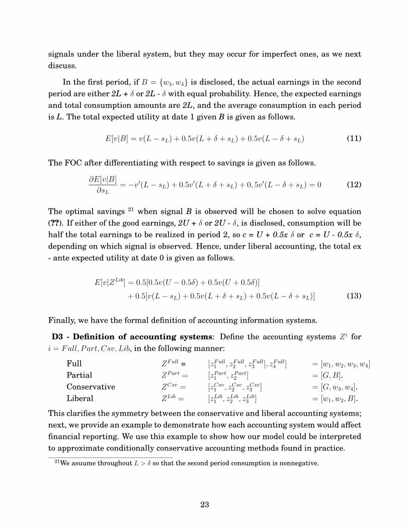


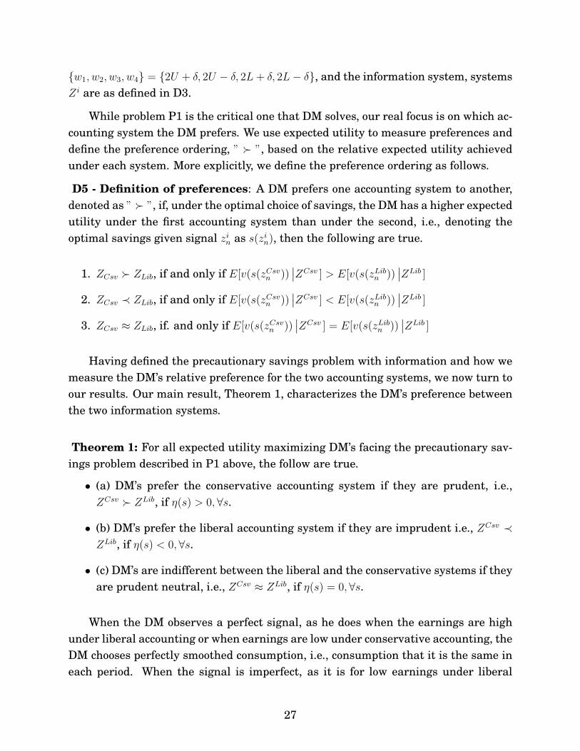


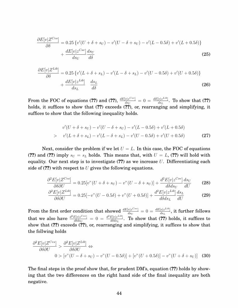

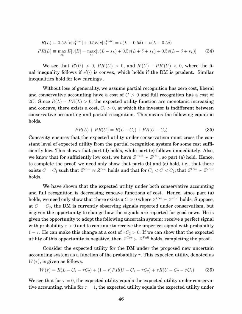


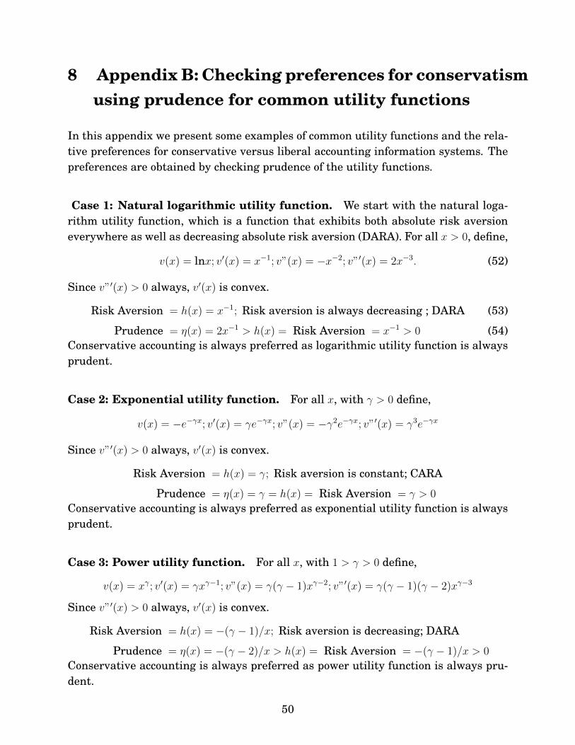


![looselywoven.orglooselywoven.org/concerts/prudence/music/Prudence Music Maria Full... · The colour of Prudence [July 2009] Please don’t disturb Dear Prudence ...](https://static.documents.pub/doc/80x56/5ac0c5187f8b9aca388c4f0c/music-maria-fullthe-colour-of-prudence-july-2009-please-dont-disturb-dear.jpg)


