Pseudonormality and a Lagrange Multiplier Theory for ... 2000 Submitted for publication to JOTA...

November 2000 Submitted for publication to JOTA

Pseudonormality and a Lagrange Multiplier Theory

for Constrained Optimization1

by

Dimitri P. Bertsekas and Asuman E. Ozdaglar2

Abstract

We consider optimization problems with equality, inequality, and abstract set constraints,and we explore various characteristics of the constraint set that imply the existence of Lagrangemultipliers. We prove a generalized version of the Fritz-John theorem, and we introduce newand general conditions that extend and unify the major constraint qualifications. Among theseconditions, two new properties, pseudonormality and quasinormality, emerge as central withinthe taxonomy of interesting constraint characteristics. In the case where there is no abstract setconstraint, these properties provide the connecting link between the classical constraint quali-fications and two distinct pathways to the existence of Lagrange multipliers: one involving thenotion of quasiregularity and Farkas’ Lemma, and the other involving the use of exact penaltyfunctions. The second pathway also applies in the general case where there is an abstract setconstraint.

1 Research supported by NSF under Grant ACI-9873339.2 Dept. of Electrical Engineering and Computer Science, M.I.T., Cambridge, Mass., 02139.

1

1. Introduction

1. INTRODUCTION

We consider finite-dimensional optimization problems of the form

minimize f(x)

subject to x ∈ C,(1.1)

where the constraint set C consists of equality and inequality constraints as well as an additional

abstract set constraint x ∈ X:

C = X ∩{x | h1(x) = 0, . . . , hm(x) = 0

}∩

{x | g1(x) ≤ 0, . . . , gr(x) ≤ 0

}. (1.2)

We assume throughout the paper that f , hi, gj are smooth (continuously differentiable) functions

from �n to �, and X is a nonempty closed set. In our notation, all vectors are viewed as column

vectors, and a prime denotes transposition, so x′y denotes the inner product of the vectors x and

y. We will use throughout the standard Euclidean norm ‖x‖ = (x′x)1/2.

Necessary conditions for the above problem can be expressed in terms of tangent cones,

normal cones, and their polars. In our terminology, a vector y is a tangent of a set S ⊂ �n at a

vector x ∈ S if either y = 0 or there exists a sequence {xk} ⊂ S such that xk �= x for all k and

xk → x,xk − x

‖xk − x‖ → y

‖y‖ .

An equivalent definition often found in the literature (e.g., Bazaraa, Sherali, and Shetty [BSS93],

Rockafellar and Wets [RoW98]) is that there exist a sequence {xk} ⊂ S with xk → x, and a

positive sequence {αk} such that αk → 0 and (xk − x)/αk → y. The set of all tangents of S at x

is denoted by TS(x) and is also referred to as the tangent cone of S at x. The polar cone of any

cone T is defined by

T ∗ ={z | z′y ≤ 0, y ∈ T

}.

For a nonempty cone T , we will use the well-known relation T ⊂(T ∗

)∗, which holds with equality

if T is closed and convex.

For a closed set X and a point x ∈ X, we will also use the normal cone of X at x, denoted

by NX(x), which is obtained from the polar cone TX(x)∗ by means of a closure operation. In

particular, we have z ∈ NX(x) if there exist sequences {xk} ⊂ X and {zk} such that xk → x,

zk → z, and zk ∈ TX(xk)∗ for all k. Equivalently, the graph of NX(·), viewed as a point-to-

set mapping,{(x, z) | z ∈ NX(x)

}, is the closure of the graph of TX(·)∗. The normal cone,

introduced by Mordukhovich [Mor76], has been studied by several authors, and is of central

importance in nonsmooth analysis (see the books by Aubin and Frankowska [AuF90], Rockafellar

2

1. Introduction

and Wets [RoW98], and Borwein and Lewis [BoL00]; for the case where X is a closed subset of

�n, our definition of NX(x) coincides with the ones used by these authors). In general, we have

TX(x)∗ ⊂ NX(x) for any x ∈ X. However, NX(x) may not be equal to TX(x)∗, and in fact it

may not even be a convex set. In the case where TX(x)∗ = NX(x), we will say that X is regular

at x. The term “regular at x in the sense of Clarke” is also used in the literature (see, Rockafellar

and Wets [RoW98], p. 199). Two properties of regularity that are important for our purposes are

that (1) if X is convex, then it is regular at each x ∈ X, and (2) if X is regular at some x ∈ X,

then TX(x) is convex (Rockafellar and Wets [RoW98], pp. 203 and 221).

A classical necessary condition for a vector x∗ ∈ C to be a local minimum of f over C is

∇f(x∗)′y ≥ 0, ∀ y ∈ TC(x∗), (1.3)

where TC(x∗) is the tangent cone of C at x∗ (see e.g., Bazaraa, Sherali, and Shetty [BSS93], Bert-

sekas [Ber99], Hestenes [Hes75], Rockafellar [Roc93], Rockafellar and Wets [RoW98]). Necessary

conditions that involve Lagrange multipliers relate to the specific representation of the constraint

set C in terms of the constraint functions hi and gj . In particular, we say that the constraint set

C of Eq. (1.2) admits Lagrange multipliers at a point x∗ ∈ C if for every smooth cost function

f for which x∗ is a local minimum of problem (1.1) there exist vectors λ∗ = (λ∗1, . . . , λ

∗m) and

µ∗ = (µ∗1, . . . , µ

∗r) that satisfy the following conditions:

∇f(x∗) +m∑

i=1

λ∗i∇hi(x∗) +

r∑j=1

µ∗j∇gj(x∗)

′

y ≥ 0, ∀ y ∈ TX(x∗), (1.4)

µ∗j ≥ 0, ∀ j = 1, . . . , r, (1.5)

µ∗j = 0, ∀ j /∈ A(x∗), (1.6)

where A(x∗) ={j | gj(x∗) = 0

}is the index set of inequality constraints that are active at

x∗. Condition (1.6) is referred to as the complementary slackness condition (CS for short). A

pair (λ∗, µ∗) satisfying Eqs. (1.4)-(1.6) will be called a Lagrange multiplier vector corresponding

to f and x∗. When there is no danger of confusion, we refer to (λ∗, µ∗) simply as a Lagrange

multiplier vector or a Lagrange multiplier . We observe that the set of Lagrange multiplier vectors

corresponding to a given f and x∗ is a (possibly empty) closed and convex set.

The condition (1.4) is consistent with the traditional characteristic property of Lagrange

multipliers: rendering the Lagrangian function stationary at x∗ [cf. Eq. (1.3)]. When X is a

convex set, Eq. (1.4) is equivalent to∇f(x∗) +

m∑i=1

λ∗i∇hi(x∗) +

r∑j=1

µ∗j∇gj(x∗)

′

(x − x∗) ≥ 0, ∀ x ∈ X. (1.7)

3

1. Introduction

This is because when X is convex, TX(x∗) is equal to the closure of the set of feasible directions

FX(x∗), which is in turn equal to the set of vectors of the form α(x − x∗), where α > 0 and

x ∈ X. If X = �n, Eq. (1.7) becomes

∇f(x∗) +m∑

i=1

λ∗i∇hi(x∗) +

r∑j=1

µ∗j∇gj(x∗) = 0,

which together with the nonnegativity condition (1.5) and the CS condition (1.6), comprise the

familiar Karush-Kuhn-Tucker conditions.

In the case where X = �n, it is well-known (see e.g., Bertsekas [Ber99], p. 332) that for a

given smooth f for which x∗ is a local minimum, there exist Lagrange multipliers if and only if

∇f(x∗)′y ≥ 0, ∀ y ∈ V (x∗),

where V (x∗) is the cone of first order feasible variations at x∗, given by

V (x∗) ={y | ∇hi(x∗)′y = 0, i = 1, . . . , m, ∇gj(x∗)′y ≤ 0, j ∈ A(x∗)

}.

This result, a direct consequence of Farkas’ Lemma, leads to the classical theorem that the

constraint set admits Lagrange multipliers at x∗ if TC(x∗) = V (x∗). In this case we say that

x∗ is a quasiregular point or that quasiregularity holds at x∗ [other terms used are x∗ “satisfies

Abadie’s constraint qualification” (Abadie [Aba67], Bazaraa, Sherali, and Shetty [BSS93]), or “is

a regular point” (Hestenes [Hes75])].

Since quasiregularity is a somewhat abstract property, it is useful to have more readily veri-

fiable conditions for the admittance of Lagrange multipliers. Such conditions are called constraint

qualifications, and have been investigated extensively in the literature. Some of the most useful

ones are the following:

CQ1: X = �n and x∗ is a regular point in the sense that the equality constraint gradients ∇hi(x∗),

i = 1, . . . , m, and the active inequality constraint gradients ∇gj(x∗), j ∈ A(x∗), are linearly

independent.

CQ2: X = �n, the equality constraint gradients ∇hi(x∗), i = 1, . . . , m, are linearly independent,

and there exists a y ∈ �n such that

∇hi(x∗)′y = 0, i = 1, . . . , m, ∇gj(x∗)′y < 0, ∀ j ∈ A(x∗).

For the case where there are no equality constraints, this is known as the Arrow-Hurwitz-

Uzawa constraint qualification, introduced in [AHU61]. In the more general case where there

4

1. Introduction

are equality constraints, it is known as the Mangasarian-Fromovitz constraint qualification,

introduced in [MaF67].

CQ3: X = �n, the functions hi are linear and the functions gj are concave.

It is well-known that all of the above constraint qualifications imply the quasiregularity

condition TC(x∗) = V (x∗), and therefore imply that the constraint set admits Lagrange multi-

pliers (see e.g., Bertsekas [Ber99], or Bazaraa, Sherali, and Shetty [BSS93]; a survey of constraint

qualifications is given by Peterson [Pet73]). These results constitute the classical pathway to

Lagrange multipliers for the case where X = �n.

However, there is another equally powerful approach to Lagrange multipliers, based on exact

penalty functions, which has not received much attention thus far. In particular, let us say that

the constraint set C admits an exact penalty at the feasible point x∗ if for every smooth function

f for which x∗ is a strict local minimum of f over C, there is a scalar c > 0 such that x∗ is also

a local minimum of the function

Fc(x) = f(x) + c

m∑

i=1

|hi(x)| +r∑

j=1

g+j (x)

over x ∈ X, where we denote

g+j (x) = max

{0, gj(x)

}.

Note that, like admittance of Lagrange multipliers, admittance of an exact penalty is a property

of the constraint set C, and does not depend on the cost function f of problem (1.1).

We intend to use exact penalty functions as a vehicle towards asserting the admittance of

Lagrange multipliers. For this purpose, there is no loss of generality in requiring that x∗ be a strict

local minimum, since we can replace a cost function f(x) with the cost function f(x)+ ‖x−x∗‖2

without affecting the problem’s Lagrange multipliers. On the other hand if we allow functions f

involving multiple local minima, it is hard to relate constraint qualifications such as the preceding

ones, the admittance of an exact penalty, and the admittance of Lagrange multipliers, as we show

in Example 11 of Section 7.

Note two important points, which illustrate the significance of exact penalty functions as a

unifying vehicle towards guaranteeing the admittance of Lagrange multipliers.

(a) If X is convex and the constraint set admits an exact penalty at x∗ it also admits Lagrange

multipliers at x∗. (This follows from Prop. 3.112 of Bonnans and Shapiro [BoS00]; see also

the subsequent Prop. 8, which generalizes the Bonnans-Shapiro result by assuming that X

is regular at x∗ instead of being convex.)

5

1. Introduction

(b) All of the above constraint qualifications CQ1-CQ3 imply that C admits an exact penalty.

(The case of CQ1 was treated by Pietrzykowski [Pie69]; the case of CQ2 was treated by

Zangwill [Zan67], Han and Mangasarian [HaM79], and Bazaraa and Goode [BaG82]; the

case of CQ3 will be dealt with in the present paper – see the subsequent Props. 3 and 9.)

Regularity

Admittance of LagrangeMultipliers

Linear/ConcaveConstraints

Mangasarian-FromovitzConstraint Qualification

Quasiregularity Admittance of an ExactPenalty

X = Rn

Figure 1. Characterizations of the constraint set C that imply admittance of Lagrange multi-

pliers in the case where X = �n.

Figure 1 summarizes the relationships discussed above for the case X = �n, and highlights

the two distinct pathways to the admittance of Lagrange multipliers. The two key notions,

quasiregularity and admittance of an exact penalty, do not seem to be directly related (see

Examples 6 and 7 in Section 7), but we will show in this paper that they are connected through

the new notion of constraint pseudonormality , which implies both while being implied by the

constraint qualifications CQ1-CQ3. Another similar connecting link is the notion of constraint

quasinormality , which is implied by pseudonormality.

Unfortunately, when X is a strict subset of �n the situation changes significantly because

there does not appear to be a satisfactory extension of the notion of quasiregularity, which

implies admittance of Lagrange multipliers. For example, the classical constraint qualification of

Guignard [Gui69] resembles quasiregularity, but requires additional conditions that are not easily

verifiable. In particular, Guignard ([Gui69], Th. 2) has shown that the constraint set admits

6

1. Introduction

Lagrange multipliers at x∗ if

V (x∗) ∩ conv(TX(x∗)

)= conv

(TC(x∗)

), (1.8)

and the vector sum V (x∗)∗ + TX(x∗)∗ is a closed set [here conv(S) denotes the closure of the

convex hull of a set S]. Guignard’s conditions are equivalent to

V (x∗)∗ + TX(x∗)∗ = TC(x∗)∗,

which in turn can be shown to be a necessary and sufficient condition for the admittance of

Lagrange multipliers at x∗ based on the classical results of Gould and Tolle [GoT71], [GoT72].

In the special case where X = �n, we have TX(x∗) = �n, TX(x∗)∗ = {0}, and the condition

(1.8) becomes V (x∗) = conv(TC(x∗)

)[or equivalently V (x∗)∗ = TC(x∗)∗], which is a similar but

slightly less restrictive constraint qualification than quasiregularity. However, in the more general

case where X �= �n, condition (1.8) and the closure of the set V (x∗)∗ + TX(x∗)∗ seem hard to

verify. (Guignard [Gui69] has only treated the cases where X is either �n or the nonnegative

orthant.)

In this paper, we focus on the connections between constraint qualifications, Lagrange

multipliers, and exact penalty functions. Much of our analysis is motivated by an enhanced set

of Fritz John necessary conditions that are introduced in the next section. Weaker versions of

these conditions were shown in a largely overlooked analysis by Hestenes [Hes75] for the case

where X = �n, and in the first author’s recent textbook [Ber99] for the case where X is a closed

convex set (see the discussion in Section 2). They are strengthened and further generalized in

Section 2 for the case where X is a closed but not necessarily convex set. In particular, we show

the existence of Fritz-John multipliers that satisfy some additional sensitivity-like conditions.

These conditions motivate the introduction of two new types of Lagrange multipliers, called

informative and strong . We show that informative and strong Lagrange multipliers exist when

the tangent cone is convex and the set of Lagrange multipliers is nonempty.

In Section 3, we introduce the notions of pseudonormality and quasinormality, and we

discuss their connection with classical results relating constraint qualifications and the admittance

of Lagrange multipliers. Quasinormality serves almost the same purpose as pseudonormality when

X is regular, but fails to provide the desired theoretical unification when X is not regular (compare

with Fig. 6). For this reason, it appears that pseudonormality is a theoretically more interesting

notion than quasinormality. In addition, in contrast with quasinormality, pseudonormality admits

an insightful geometrical interpretation. In Section 3, we also introduce a new and natural

extension of the Mangasarian-Fromovitz constraint qualification, which applies to the case where

X �= �n and implies pseudonormality.

7

2. Enhanced Fritz John Conditions

In Section 4, we make the connection between pseudonormality, quasinormality, and exact

penalty functions. In particular, we show that pseudonormality implies the admittance of an

exact penalty, while being implied by the major constraint qualifications. In the process we

prove in a unified way that the constraint set admits an exact penalty for a much larger variety of

constraint qualifications than has been known hitherto. We note that exact penalty functions have

traditionally been viewed as a computational device and they have not been earlier integrated

within the theory of constraint qualifications in the manner described here. Let us also note

that exact penalty functions are related to the notion of calmness, introduced and suggested as a

constraint qualification by Clarke [Cla76], [Cla83]. However, there are some important differences

between the notions of calmness and admittance of an exact penalty. In particular, calmness is

a property of the problem (1.1) and depends on the cost function f , while admittance of an

exact penalty is a property of the constraint set and is independent of the cost function. More

importantly for the purposes of this paper, calmness is not useful as a unifying theoretical vehicle

because it does not relate well with other major constraint qualifications. For example CQ1, one

of the most common constraint qualifications, does not imply calmness of problem (1.1), as is

indicated by Example 11 of Section 7, and reversely, calmness of the problem does not imply

CQ1.

In Section 5, we discuss some special results that facilitate proofs of admittance of Lagrange

multipliers and of an exact penalty. In Section 6, we generalize some of our analysis to the case

of a convex programming problem and we provide a geometric interpretation of pseudonormality.

Finally, in Section 7 we provide examples and counterexamples that clarify the interrelations

between the different characterizations that we have introduced.

2. ENHANCED FRITZ JOHN CONDITIONS

The Fritz John necessary optimality conditions [Joh48] are often used as the starting point for the

analysis of Lagrange multipliers. Unfortunately, these conditions in their classical form are not

sufficient to derive the admittance of Lagrange multipliers under some of the standard constraint

qualifications, such as when X = �n and the constraint functions hi and gj are linear (cf. CQ3).

Recently, the classical Fritz John conditions have been strengthened through the addition of an

extra necessary condition, and their effectiveness has been significantly enhanced (see Hestenes

[Hes75] for the case X = �n, and Bertsekas [Ber99], Prop. 3.3.11, for the case where X is a

closed convex set). The following proposition extends these results by allowing the set X to be

nonconvex, and by also showing that the Fritz John multipliers can be selected to have some

special sensitivity-like properties [see condition (iv) below].

8


Proposition 1: Let x∗ be a local minimum of problem (1.1)-(1.2). Then there exist scalars

µ∗0, λ∗

1, . . . , λ∗m, and µ∗

1, . . . , µ∗r , satisfying the following conditions:

(i) −(µ∗

0∇f(x∗) +∑m

i=1 λ∗i∇hi(x∗) +

∑rj=1 µ∗

j∇gj(x∗))∈ NX(x∗).

(ii) µ∗j ≥ 0 for all j = 0, 1, . . . , r.

(iii) µ∗0, λ

∗1, . . . , λ

∗m, µ∗

1, . . . , µ∗r are not all equal to 0.

(iv) If the index set I ∪ J is nonempty where

I = {i | λ∗i �= 0}, J = {j �= 0 | µ∗

j > 0},

there exists a sequence {xk} ⊂ X that converges to x∗ and is such that for all k,

f(xk) < f(x∗), λ∗i hi(xk) > 0, ∀ i ∈ I, µ∗

jgj(xk) > 0, ∀ j ∈ J, (2.1)

|hi(xk)| = o(w(xk)

), ∀ i /∈ I, g+

j (xk) = o(w(xk)

), ∀ j /∈ J, (2.2)

where

w(x) = min{

mini∈I

|hi(x)|, minj∈J

gj(x)}

. (2.3)

Proof: We use a quadratic penalty function approach. For each k = 1, 2, . . ., consider the

“penalized” problem

minimize F k(x) ≡ f(x) +k

2

m∑i=1

(hi(x)

)2 +k

2

r∑j=1

(g+

j (x))2 +

12||x − x∗||2

subject to x ∈ X ∩ S,

where S = {x | ||x − x∗|| ≤ ε}, and ε > 0 is such that f(x∗) ≤ f(x) for all feasible x with x ∈ S.

Since X ∩ S is compact, by Weierstrass’ theorem, we can select an optimal solution xk of the

above problem. We have for all k

f(xk) +k

2

m∑i=1

(hi(xk)

)2 +k

2

r∑j=1

(g+

j (xk))2 +

12||xk − x∗||2 = F k(xk) ≤ F k(x∗) = f(x∗) (2.4)

and since f(xk) is bounded over X ∩ S, we obtain

limk→∞

|hi(xk)| = 0, i = 1, . . . , m, limk→∞

|g+j (xk)| = 0, j = 1, . . . , r;

otherwise the left-hand side of Eq. (2.4) would become unbounded from above as k → ∞.

Therefore, every limit point x of {xk} is feasible, i.e., x ∈ C. Furthermore, Eq. (2.4) yields

f(xk) + (1/2)||xk − x∗||2 ≤ f(x∗) for all k, so by taking the limit as k → ∞, we obtain

f(x) +12||x − x∗||2 ≤ f(x∗).

9


Since x ∈ S and x is feasible, we have f(x∗) ≤ f(x), which when combined with the preceding

inequality yields ||x − x∗|| = 0 so that x = x∗. Thus the sequence {xk} converges to x∗, and it

follows that xk is an interior point of the closed sphere S for all k greater than some k.

For k ≥ k, we have by the necessary condition (1.3), ∇F k(xk)′y ≥ 0 for all y ∈ TX(xk), or

equivalently −∇F k(xk) ∈ TX(xk)∗, which is written as

−

∇f(xk) +

m∑i=1

ξki ∇hi(xk) +

r∑j=1

ζkj ∇gj(xk) + (xk − x∗)

∈ TX(xk)∗, (2.5)

where

ξki = khi(xk), ζk

j = kg+j (xk). (2.6)

Denote,

δk =

√√√√1 +m∑

i=1

(ξki )2 +

r∑j=1

(ζkj )2, (2.7)

µk0 =

1δk

, λki =

ξki

δk, i = 1, . . . , m, µk

j =ζkj

δk, j = 1, . . . , r. (2.8)

Then by dividing Eq. (2.5) with δk, we obtain

−

µk

0∇f(xk) +m∑

i=1

λki ∇hi(xk) +

r∑j=1

µkj∇gj(xk) +

1δk

(xk − x∗)

∈ TX(xk)∗. (2.9)

Since by construction we have

(µk0)2 +

m∑i=1

(λki )2 +

r∑j=1

(µkj )2 = 1, eqnum

the sequence {µk0 , λk

1 , . . . , λkm, µk

1 , . . . , µkr} is bounded and must contain a subsequence that con-

verges to some limit {µ∗0, λ

∗1, . . . , λ

∗m, µ∗

1, . . . , µ∗r}.

From Eq. (2.9) and the defining property of the normal cone NX(x∗) [xk → x∗, {xk} ⊂ X,

zk → z∗, and zk ∈ TX(xk)∗ for all k, imply that z∗ ∈ NX(x∗)], we see that µ∗0, λ∗

i , and µ∗j

must satisfy condition (i). From Eqs. (2.6) and (2.8), µ∗0 and µ∗

j must satisfy condition (ii), and

from Eq. (2.10), µ∗0, λ∗

i , and µ∗j must satisfy condition (iii). Finally, to show that condition (iv)

is satisfied, assume that I ∪ J is nonempty, and note that for all sufficiently large k within the

index set K of the convergent subsequence, we must have λ∗i λ

ki > 0 for all i ∈ I and µ∗

jµkj > 0

for all j ∈ J . Therefore, for these k, from Eqs. (2.6) and (2.8), we must have λ∗i hi(xk) > 0 for

all i ∈ I and µ∗jgj(xk) > 0 for all j ∈ J , while from Eq. (2.4), we have f(xk) < f(x∗) for k

sufficiently large (the case where xk = x∗ for infinitely many k is excluded by the assumption

10


that I ∪ J is nonempty). Furthermore, the conditions |hi(xk)| = o(w(xk)

)for all i /∈ I, and

g+j (xk) = o

(w(xk)

)for all j /∈ J are equivalent to

|λki | = o

(min

{mini∈I

|λki |, min

j∈Jµk

j

}), ∀ i /∈ I,

and

µkj = o

(min

{mini∈I

|λki |, min

j∈Jµk

j

}), ∀ j /∈ J,

respectively, so they hold for k ∈ K. This proves condition (iv). Q.E.D.

Note that if X is regular at x∗, i.e., NX(x∗) = TX(x∗)∗, condition (i) of Prop. 1 becomes

−

µ∗

0∇f(x∗) +m∑

i=1

λ∗i∇hi(x∗) +

r∑j=1

µ∗j∇gj(x∗)

∈ TX(x∗)∗,

or equivalentlyµ∗

0∇f(x∗) +m∑

i=1

λ∗i∇hi(x∗) +

r∑j=1

µ∗j∇gj(x∗)

′

y ≥ 0, ∀ y ∈ TX(x∗).

If in addition, the scalar µ∗0 can be shown to be strictly positive, then by normalization we can

choose µ∗0 = 1, and condition (i) of Prop. 1 becomes equivalent to the Lagrangian stationarity

condition (1.4). Thus, if X is regular at x∗ and we can guarantee that µ∗0 = 1, the vector

(λ∗, µ∗) = {λ∗1, . . . , λ

∗m, µ∗

1, . . . , µ∗r} is a Lagrange multiplier vector that satisfies condition (iv) of

Prop. 1. A key fact is that this condition is stronger than the CS condition (1.6). [If µ∗j > 0,

then according to condition (iv), the corresponding jth inequality constraint must be violated

arbitrarily close to x∗ [cf. Eq. (2.1)], implying that gj(x∗) = 0.] For ease of reference, we refer

to condition (iv) as the complementary violation condition (CV for short).† This condition will

turn out to be of crucial significance in the next section.

To place Prop. 1 in perspective, we note that its line of proof, based on the quadratic

penalty function, originated with McShane [McS73]. Hestenes [Hes75] observed that McShane’s

proof can be used to strengthen the CS condition to assert the existence of a sequence {xk} such

that

λ∗i hi(xk) > 0, ∀ i ∈ I, µ∗

jgj(xk) > 0, ∀ j ∈ J, (2.10)

which is slightly weaker than CV as defined here [there is no requirement that xk, simultaneously

with violation of the constraints with nonzero multipliers, satisfies f(xk) < f(x∗) and Eq. (2.2)].

† This term is in analogy with “complementary slackness,” which is the condition that for all j,

µ∗j > 0 implies gj(x

∗) = 0. Thus “complementary violation” reflects the condition that for all j, µ∗j > 0

implies gj(x) > 0 for some x arbitrarily close to x∗ (and simultaneously for all j with µ∗j > 0).

11


McShane and Hestenes considered only the case where X = �n. The case where X is a closed

convex set was considered in Bertsekas [Ber99], where a generalized version of the Mangasarian-

Fromovitz constraint qualification was also proved. The extension to the case where X is a

general closed set and the strengthened version of condition (iv) are given in the present paper

for the first time.

To illustrate the use of the generalized Fritz John conditions of Prop. 1 and the CV condition

in particular, consider the following example.

Example 1

Suppose that we convert a problem with a single equality constraint, minh(x)=0 f(x), to the in-

equality constrained problem

minimize f(x)

subject to h(x) ≤ 0, −h(x) ≤ 0.

The Fritz John conditions assert the existence of nonnegative µ∗0, λ

+, λ−, not all zero, such that

µ∗0∇f(x∗) + λ+∇h(x∗) − λ−∇h(x∗) = 0. (2.11)

The candidate multipliers that satisfy the above condition as well as the CS condition λ+h(x∗) =

λ−h(x∗) = 0, include those of the form µ∗0 = 0 and λ+ = λ− > 0, which provide no relevant

information about the problem. However, these multipliers fail the stronger CV condition of Prop.

1, showing that if µ∗0 = 0, we must have either λ+ �= 0 and λ− = 0 or λ+ = 0 and λ− �= 0. Assuming

∇h(x∗) �= 0, this violates Eq. (2.11), so it follows that µ∗0 > 0. Thus, by dividing Eq. (2.11) by

µ∗0, we recover the familiar first order condition ∇f(x∗) + λ∗∇h(x∗) = 0 with λ∗ = (λ+ − λ−)/µ∗

0,

under the regularity assumption ∇h(x∗) �= 0. Note that this deduction would not have been

possible without the CV condition.

If we can take µ∗0 = 1 in Prop. 1 for all smooth f for which x∗ is a local minimum, and X is

regular at x∗, then the constraint set C admits Lagrange multipliers of a special type, which satisfy

the stronger CV condition in place of the CS condition. The salient feature of such multipliers is

the information they embody regarding constraint violation with corresponding cost reduction.

This is consistent with the classical sensitivity interpretation of a Lagrange multiplier as the rate

of reduction in cost as the corresponding constraint is violated. Here we are not making enough

assumptions for this stronger type of sensitivity interpretation to be valid. Yet it is remarkable

that with hardly any assumptions (other than their existence), Lagrange multipliers of the type

obtained through Prop. 1, provide a significant amount of sensitivity information: they indicate

the index set I ∪ J of constraints that if violated, a cost reduction can be effected [the remaining

constraints, whose indices do not belong to I ∪ J , may also be violated, but the degree of their

12


violation is arbitrarily small relative to the other constraints as per Eqs. (2.2) and (2.3)]. In view

of this interpretation, we refer to a Lagrange multiplier vector (λ∗, µ∗) that satisfies, in addition

to Eqs. (1.4)-(1.6), the CV condition [condition (iv) of Prop. 1] as being informative.

An informative Lagrange multiplier vector is useful, among other things, if one is interested

in identifying redundant constraints. Given such a vector, one may simply discard the constraints

whose multipliers are 0 and check to see whether x∗ is still a local minimum. While there is no

general guarantee that this will be true, in many cases it will be; for example, in the special case

where f and X are convex, the gj are convex, and the hi are linear, x∗ is guaranteed to be a

global minimum, even after the constraints whose multipliers are 0 are discarded.

Now if we are interested in discarding constraints whose multipliers are 0, we are also

motivated to find Lagrange multiplier vectors that have a minimal number of nonzero components

(a minimal support). We call such Lagrange multiplier vectors minimal , and we define them as

having support I ∪ J that does not strictly contain the support of any other Lagrange multiplier

vector. Minimal Lagrange multipliers are not necessarily informative. For example, think of the

case where some of the constraints are duplicates of others. Then in a minimal Lagrange multiplier

vector, at most one of each set of duplicate constraints can have a nonzero multiplier, while in

an informative Lagrange multiplier vector, either all or none of these duplicate constraints will

have a nonzero multiplier. Nonetheless, minimal Lagrange multipliers turn out to be informative

after the constraints corresponding to zero multipliers are neglected, as can be inferred by the

subsequent Prop. 2. In particular, let us say that a Lagrange multiplier (λ∗, µ∗) is strong if in

addition to Eqs. (1.4)-(1.6), it satisfies the condition

(iv′) If the set I ∪ J is nonempty, where I = {i | λ∗i �= 0} and J = {j �= 0 | µ∗

j > 0}, then given

any neighborhood B of x∗, there exists a sequence {xk} ⊂ X that converges to x∗ and is

such that for all k,

f(xk) < f(x∗), λ∗i hi(xk) > 0, ∀ i ∈ I, gj(xk) > 0, ∀ j ∈ J. (2.12)

This condition resembles the CV condition, but is weaker in that it makes no provision for

negligibly small violation of the constraints corresponding to zero multipliers, as per Eqs. (2.2)

and (2.3). As a result, informative Lagrange multipliers are also strong, but not reversely.

The following proposition, illustrated in Fig. 2, clarifies the relationships between different

types of Lagrange multipliers.

Proposition 2: Let x∗ be a local minimum of problem (1.1)-(1.2). Assume that the tangent

cone TX(x∗) is convex and that the set of Lagrange multipliers is nonempty. Then:

13


Lagrange multipliers

Strong

Informative Minimal

Figure 2. Relations of different types of Lagrange multipliers, assuming that the tangent cone

TX(x∗) is convex (which is true in particular if X is regular at x∗).

(a) The set of informative Lagrange multiplier vectors is nonempty, and in fact the Lagrange

multiplier vector that has minimum norm is informative.

(b) Each minimal Lagrange multiplier vector is strong.

Proof: (a) We summarize the essence of the proof argument in the following lemma (a related

but different line of proof of this lemma is given in [BNO01]).

Lemma 1: Let N be a closed convex cone in �n, and let a0, a1, . . . , ar be given vectors in �n.

Suppose that the closed and convex set M ⊂ �r given by

M =

µ ≥ 0

∣∣∣ −

a0 +

r∑j=1

µjaj

∈ N

,

is nonempty. Then there exists a sequence {dk} ⊂ N∗ such that

a′0d

k → −‖µ∗‖2, (2.13)

(a′jd

k)+ → µ∗j , j = 1, . . . , r, (2.14)

where µ∗ is the vector of minimum norm in M .

Proof: For any γ ≥ 0, consider the function

Lγ(d, µ) =

a0 +

r∑j=1

µjaj

′

d + γ‖d‖ − 12‖µ‖2.

Our proof will revolve around saddle point properties of the convex/concave function L0, but to

derive these properties, we will work with its γ-perturbed and coercive version Lγ for γ > 0, and

then take the limit as γ → 0. With this in mind, we first establish that if γ > 0, Lγ(d, µ) has a

saddle point over d ∈ N∗ and µ ≥ 0.

14


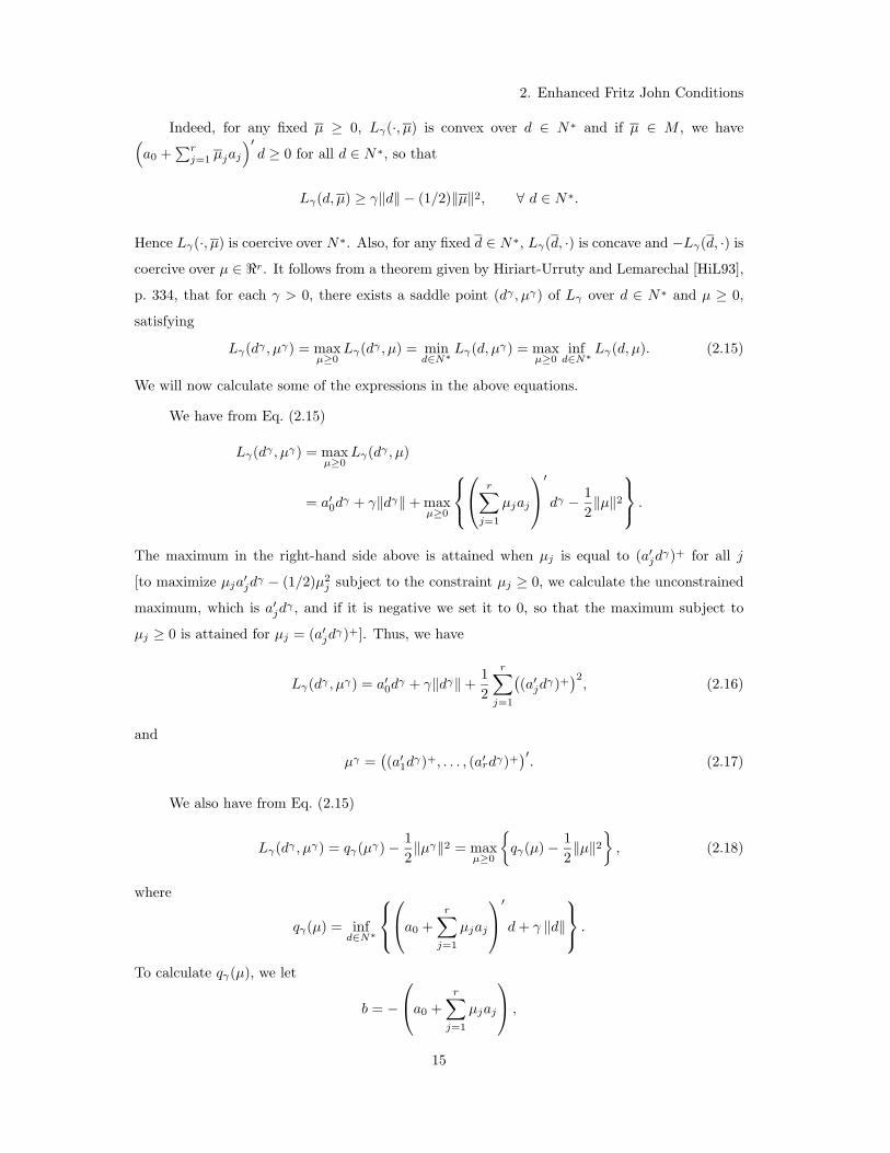
Indeed, for any fixed µ ≥ 0, Lγ(·, µ) is convex over d ∈ N∗ and if µ ∈ M , we have(a0 +

∑rj=1 µjaj

)′d ≥ 0 for all d ∈ N∗, so that

Lγ(d, µ) ≥ γ‖d‖ − (1/2)‖µ‖2, ∀ d ∈ N∗.

Hence Lγ(·, µ) is coercive over N∗. Also, for any fixed d ∈ N∗, Lγ(d, ·) is concave and −Lγ(d, ·) is

coercive over µ ∈ �r. It follows from a theorem given by Hiriart-Urruty and Lemarechal [HiL93],

p. 334, that for each γ > 0, there exists a saddle point (dγ , µγ) of Lγ over d ∈ N∗ and µ ≥ 0,

satisfying

Lγ(dγ , µγ) = maxµ≥0

Lγ(dγ , µ) = mind∈N∗

Lγ(d, µγ) = maxµ≥0

infd∈N∗

Lγ(d, µ). (2.15)

We will now calculate some of the expressions in the above equations.

We have from Eq. (2.15)

Lγ(dγ , µγ) = maxµ≥0

Lγ(dγ , µ)

= a′0d

γ + γ‖dγ‖ + maxµ≥0

r∑

j=1

µjaj

′

dγ − 12‖µ‖2

.

The maximum in the right-hand side above is attained when µj is equal to (a′jd

γ)+ for all j

[to maximize µja′jd

γ − (1/2)µ2j subject to the constraint µj ≥ 0, we calculate the unconstrained

maximum, which is a′jd

γ , and if it is negative we set it to 0, so that the maximum subject to

µj ≥ 0 is attained for µj = (a′jd

γ)+]. Thus, we have

Lγ(dγ , µγ) = a′0d

γ + γ‖dγ‖ +12

r∑j=1

((a′

jdγ)+

)2, (2.16)

and

µγ =((a′

1dγ)+, . . . , (a′

rdγ)+)′

. (2.17)

We also have from Eq. (2.15)

Lγ(dγ , µγ) = qγ(µγ) − 12‖µγ‖2 = max

µ≥0

{qγ(µ) − 1

2‖µ‖2

}, (2.18)

where

qγ(µ) = infd∈N∗

a0 +

r∑j=1

µjaj

′

d + γ ‖d‖

.

To calculate qγ(µ), we let

b = −

a0 +

r∑j=1

µjaj

,

15


and we use the transformation d = αξ, where α ≥ 0 and ‖ξ‖ = 1, to write

qγ(µ) = infα≥0

‖ξ‖≤1, ξ∈N∗

{α(γ − b′ξ)

}=

{ 0 if max‖ξ‖≤1, ξ∈N∗ b′ξ ≤ γ,

−∞ otherwise.(2.19)

We will show that

max‖ξ‖≤1, ξ∈N∗

b′ξ ≤ γ if and only if b ∈ N + S(0, γ), (2.20)

where S(0, γ) is the closed sphere of radius γ that is centered at the origin. Indeed, if b ∈N + S(0, γ), then b = b + b with b ∈ N and ‖b‖ ≤ γ, and it follows that for all ξ ∈ N∗ with

‖ξ‖ ≤ 1, we have b′ξ ≤ 0 and b′ξ ≤ γ, so that

b′ξ = b′ξ + b′ξ ≤ γ,

from which we obtain

max‖ξ‖≤1, ξ∈N∗

b′ξ ≤ γ.

Conversely, assume that b′ξ ≤ γ for all ξ ∈ N∗ with ‖ξ‖ ≤ 1. If b ∈ N , then clearly b ∈ N+S(0, γ).

If b /∈ N , let b be the projection of b onto N and let b = b − b. Because N is a convex cone, the

nonzero vector b belongs to N∗ and is orthogonal to b. Since the vector ξ = b/‖b‖ belongs to N∗

and satisfies ‖ξ‖ ≤ 1, we have γ ≥ b′ξ or equivalently γ ≥ (b + b)′(b/‖b‖) = ‖b‖. Hence, b = b + b

with b ∈ N and ‖b‖ ≤ γ, implying that b ∈ N + S(0, γ), and completing the proof of Eq. (2.20).

We have thus shown [cf. Eqs. (2.19) and Eq. (2.20)] that

qγ(µ) =

{0 if −

(a0 +

∑rj=1 µjaj

)∈ N + S(0, γ),

−∞ otherwise.(2.21)

Combining this equation with Eq. (2.18), we see that µγ is the vector of minimum norm on the

set

Mγ =

µ ≥ 0

∣∣∣ −

a0 +

r∑j=1

µjaj

∈ N + S(0, γ)

.

Furthermore, from Eqs. (2.18) and (2.21), we have

Lγ(dγ , µγ) = −12‖µγ‖2,

which together with Eqs. (2.16) and (2.17), yields

a′0d

γ + γ‖dγ‖ = −‖µγ‖2. (2.22)

We now take limit in the above equation as γ → 0. We claim that µγ → µ∗. Indeed, since

µ∗ ∈ Mγ , we have ‖µγ‖ ≤ ‖µ∗‖, so that {µγ | γ > 0} is bounded. Let µ be a limit point of µγ ,

and note that µ ≥ 0 and ‖µ‖ ≤ ‖µ∗‖. We have

−r∑

j=1

µγj aj = a0 + νγ + sγ ,

16


for some vectors νγ ∈ N and sγ ∈ S(0, γ), so by taking limit as γ → 0 along the relevant

subsequence, it follows that νγ converges to some ν ∈ N , and we have

−r∑

j=1

µjaj = a0 + ν.

It follows that µ ∈ M , and since ‖µ‖ ≤ ‖µ∗‖, we obtain µ = µ∗. The preceding argument has

shown that every limit point of µγ is equal to µ∗, so µγ converges to µ∗ as γ → 0. Thus, Eq.

(2.22) yields

lim supγ→0

a′0d

γ ≤ −‖µ∗‖2. (2.23)

Consider now the function

L0(d, µ) =

a0 +

r∑j=1

µjaj

′

d − 12‖µ‖2.

We have

a′0d

γ +12

r∑j=1

((a′

jdγ)+

)2 = supµ≥0

L0(dγ , µ)

≥ supµ≥0

infd∈N∗

L0(d, µ)

≥ infd∈N∗

L0(d, µ∗).

It can be seen that

infd∈N∗

L0(d, µ) =

{− 1

2‖µ‖2 if −(a0 +

∑rj=1 µjaj

)∈ N,

−∞ otherwise.

Combining the last two equations, we have

a′0d

γ +12

r∑j=1

((a′

jdγ)+

)2 ≥ −12‖µ∗‖2,

and since (a′jd

γ)+ = µγj [cf. Eq. (2.17)],

a′0d

γ ≥ −12‖µ∗‖2 − 1

2‖µγ‖2.

Taking the limit as γ → ∞, we obtain

lim infγ→0

a′0d

γ ≥ −‖µ∗‖2,

which together with Eq. (2.23), shows that a′0d

γ → −‖µ∗‖2. Since we have also shown that

(a′jd

γ)+ = µγj → µ∗

j , the proof is complete. Q.E.D.

We now return to the proof of Prop. 2(a). For simplicity we assume that all the constraints

are inequalities that are active at x∗ (equality constraints can be handled by conversion to two

17


inequalities, and inactive inequality constraints are inconsequential in the subsequent analysis).

We will use Lemma 1 with the following identifications:

N = TX(x∗)∗, a0 = ∇f(x∗), aj = ∇gj(x∗), j = 1, . . . , r,

M = set of Lagrange multipliers,

µ∗ = Lagrange multiplier of minimum norm.

If µ∗ = 0, then µ∗ is an informative Lagrange multiplier and we are done. If µ∗ �= 0, by Lemma

1, for any ε > 0, there exists a d ∈ N∗ = TX(x∗) such that

a′0d < 0, (2.24)

a′jd > 0, ∀ j ∈ J∗, a′

jd ≤ ε minl∈J∗

a′ld, ∀ j /∈ J∗, (2.25)

where J∗ = {j | µ∗j > 0}. By suitably scaling the vector d, we can assume that ‖d‖ = 1. Let

{xk} ⊂ X be such that xk �= x∗ for all k and

xk → x∗,xk − x∗

‖xk − x∗‖ → d.

Using Taylor’s theorem for the cost function f , we have for some vector sequence ξk converging

to 0f(xk) − f(x∗) = ∇f(x∗)′(xk − x∗) + o(‖xk − x∗‖)

= ∇f(x∗)′(d + ξk

)‖xk − x∗‖ + o(‖xk − x∗‖)

= ‖xk − x∗‖(∇f(x∗)′d + ∇f(x∗)′ξk +

o(‖xk − x∗‖)‖xk − x∗‖

).

From Eq. (2.24), we have ∇f(x∗)′d < 0, so we obtain f(xk) < f(x∗) for k sufficiently large.

Using also Taylor’s theorem for the constraint functions gj , we have for some vector sequence ξk

converging to 0,

gj(xk) − gj(x∗) = ∇gj(x∗)′(xk − x∗) + o(‖xk − x∗‖)

= ∇gj(x∗)′(d + ξk

)‖xk − x∗‖ + o(‖xk − x∗‖)

= ‖xk − x∗‖(∇gj(x∗)′d + ∇gj(x∗)′ξk +

o(‖xk − x∗‖)‖xk − x∗‖

).

This, combined with Eq. (2.25), shows that for k sufficiently large, gj(xk) is bounded from below

by a constant times ‖xk − x∗‖ for all j such that µ∗j > 0 [and hence gj(x∗) = 0], and satisfies

gj(xk) ≤ o(‖xk − x∗‖) for all j such that µ∗j = 0 [and hence gj(x∗) ≤ 0]. Thus, the sequence

{xk} can be used to establish the CV condition for µ∗, and it follows that µ∗ is an informative

Lagrange multiplier.

(b) We summarize the essence of the proof argument of this part in the following lemma.

18


Lemma 2: Let N be a closed convex cone in �n, let a0, a1, . . . , ar be given vectors in �n.


M =

µ ≥ 0

∣∣∣ −

a0 +

r∑j=1

µjaj

∈ N

,

is nonempty. Among index subsets J ⊂ {1, . . . , r} such that for some µ ∈ M we have J = {j |µj > 0}, let J ⊂ {1, . . . , r} have a minimal number of elements. Then if J is nonempty, there

exists a vector d ∈ N∗ such that

a′0d < 0, a′

jd > 0, for all j ∈ J. (2.26)

Proof: We apply Lemma 1 with the vectors a1, . . . , ar replaced by the vectors aj , j ∈ J . The

subset of M given by

M =

µ ≥ 0

∣∣∣ −

a0 +

∑j∈J

µjaj

∈ N, µj = 0, ∀ j /∈ J

is nonempty by assumption. Let µ be the vector of minimum norm on M . Since J has a minimal

number of indices, we must have µj > 0 for all j ∈ J . If J is nonempty, Lemma 1 implies that

there exists a d ∈ N∗ such that Eq. (2.26) holds. Q.E.D.

Given Lemma 2, the proof of Prop. 2(b) is very similar to the corresponding part of the

proof of Prop. 2(a). Q.E.D.

Sensitivity and the Lagrange Multiplier of Minimum Norm

Let us first introduce an interesting variation of Lemma 1:

Lemma 3: Let N be a closed convex cone in �n, and let a0, . . . , ar be given vectors in �n.


M =

µ ≥ 0

∣∣∣ −

a0 +

r∑j=1

µjaj

∈ N

,

is nonempty, and let µ∗ be the vector of minimum norm on M . Then

−‖µ∗‖2 ≤ a′0d +

12

r∑j=1

((a′

jd)+)2

, ∀ d ∈ N∗.

19


Furthermore, if d is an optimal solution of the problem

minimize a′0d +

12

r∑j=1

((a′

jd)+)2

subject to d ∈ N∗,

(2.27)

we have

a′0d = −‖µ∗‖2, (a′

jd)+ = µ∗j , j = 1, . . . , r. (2.28)

Proof: From the proof of Lemma 1, we have for all γ > 0

−12‖µ∗‖2 = sup

µ≥0inf

d∈N∗L0(d, µ)

≤ infd∈N∗

supµ≥0

L0(d, µ)

= infd∈N∗

a′

0d +12

r∑j=1

((a′

jd)+)2

.

(2.29)

If d is an optimal solution of problem (2.27), we obtain

infd∈N∗

a′

0d +12

r∑j=1

((a′

jd)+)2

= a′

0d +12

r∑j=1

((a′

jd)+)2

≤ a′0d

γ +12

r∑j=1

((a′

jdγ)+

)2.

Since (according to the proof of Lemma 1) a′0d

γ → −‖µ∗‖2 and (a′jd

γ)+ → µ∗j as γ → 0, by taking

the limit above as γ → 0, we see that equality holds throughout in the two above inequalities.

Thus (d, µ∗) is a saddle point of the function L0(d, µ) over d ∈ N∗ and µ ≥ 0. It follows that µ∗

maximizes L0(d, µ) over µ ≥ 0, so that µ∗j = (a′

jd)+ for all j and −‖µ∗‖2 = α′0d. Q.E.D.

The difference between Lemmas 1 and 3 is that in Lemma 3, there is the extra assumption

that problem (2.27) has an optimal solution (otherwise the lemma is vacuous). It can be shown

that, assuming the set M is nonempty, problem (2.27) is guaranteed to have at least one solution

when N∗ is a polyhedral cone. To see this, note that problem (2.27) can be written as

minimize a′0d +

12

r∑j=1

z2j

subject to d ∈ N∗, 0 ≤ zj , a′jd ≤ zj , j = 1, . . . , r,

where the zj are auxiliary variables. Thus, if N∗ is polyhedral, then problem (2.27) is a quadratic

program with a cost function that is bounded below by Eq. (2.29), and hence it has an optimal

solution (see Bonnans and Shapiro [BeS00], Th. 3.128). Thus, when N∗ is polyhedral, Lemma 3

20


applies. An important context where this is relevant is when X = �n in which case NX(x∗)∗ =

TX(x∗) = �n, or more generally when X is polyhedral, in which case TX(x∗) is polyhedral.

Another condition that guarantees the existence of an optimal solution of problem (2.27) is that

there exists a vector µ in the set

M =

µ ≥ 0

∣∣∣ −

a0 +

r∑j=1

µjaj

∈ N

such that

−

a0 +

r∑j=1

µjaj

∈ ri(N),

where ri(N) denotes the relative interior of N . The relevant analysis, which is due to Xin Chen

(private communication), is given in [BNO01].

When problem (2.27) can be guaranteed to have an optimal solution and Lemma 3 applies,

the line of proof of Prop. 2(a) can be used to show that if the Lagrange multiplier that has

minimum norm, denoted by (λ∗, µ∗), is nonzero, there exists a sequence {xk} ⊂ X and a positive

constant c such that

f(xk) = f(x∗) −m∑

i=1

λ∗i hi(xk) −

r∑j=1

µ∗jgj(xk) + o(‖xk − x∗‖), (2.30)

hi(xk) = cλ∗i ‖xk − x∗‖ + o(‖xk − x∗‖), i = 1, . . . , m, (2.31)

gj(xk) = cµ∗j ‖xk − x∗‖ + o(‖xk − x∗‖), if µ∗

j > 0, (2.32)

gj(xk) ≤ o(‖xk − x∗‖), if µ∗j = 0. (2.33)

These equations suggest that the minimum-norm Lagrange multiplier has a sensitivity in-

terpretation. In particular, the sequence {xk} above corresponds to the vector d ∈ TX(x∗) of Eq.

(2.28), which solves problem (2.27). From this it can be seen that a positive multiple of d solves

the problem

minimize ∇f(x∗)′d

subject tom∑

i=1

(∇hi(x∗)′d

)2 +∑

j∈A(x∗)

(∇gj(x∗)′d)+

)2 = β, d ∈ TX(x∗),

for any given positive scalar β. Thus, d is the tangent direction that maximizes the cost function

improvement (calculated up to first order) for a given value of the norm of the constraint violation

(calculated up to first order). From Eq. (2.30), this first order cost improvement is equal tom∑

i=1

λ∗i hi(xk) +

r∑j=1

µ∗jgj(xk).

Thus, the multipliers λ∗i and µ∗

j express the rate of improvement per unit constraint violation,

along the maximum improvement (or steepest descent) direction d. This is consistent with the

traditional sensitivity interpretation of Lagrange multipliers.

21


An Alternative Definition of Lagrange Multipliers

Finally, let us make the connection with Rockafellar’s treatment of Lagrange multipliers from

[Roc93] and [RoW98]. Consider vectors λ∗ = (λ∗1, . . . , λ

∗m) and µ∗ = (µ∗

1, . . . , µ∗r) that satisfy the

conditions

−

∇f(x∗) +

m∑i=1

λ∗i∇hi(x∗) +

r∑j=1

µ∗j∇gj(x∗)

∈ NX(x∗), (2.34)

µ∗j ≥ 0, ∀ j = 1, . . . , r, µ∗

j = 0, ∀ j /∈ A(x∗). (2.35)

Such vectors are called “Lagrange multipliers” by Rockafellar, but in this paper we will refer to

them as R-multipliers, to distinguish them from Lagrange multipliers as we have defined them

[cf. Eqs. (1.4)-(1.6)].

When X is regular at x∗, Rockafellar’s definition and our definition coincide. In general,

however, the set of Lagrange multipliers is a (possibly strict) subset of the set of R-multipliers,

since TX(x∗)∗ ⊂ NX(x∗) with inequality holding when X is not regular at x∗. Also, the existence

of R-multipliers does not guarantee the existence of Lagrange multipliers. Furthermore, even if

Lagrange multipliers exist, none of them may be informative or strong, unless the tangent cone

is convex (cf. Prop. 2 and Example 2 given below).

Note that multipliers satisfying the enhanced Fritz John conditions of Prop. 1 with µ∗0 = 1

are R-multipliers, and they still have the extra sensitivity-like property embodied in the CV

condition. Furthermore, Lemma 1 can be used to show that assuming NX(x∗) is convex, if the

set of R-multipliers is nonempty, it contains an R-multiplier with the sensitivity-like property

of the CV condition. However, if X is not regular at x∗, an R-multiplier may not render the

Lagrangian function stationary. The following is an illustrative example.

a1a2NX(x*)

x* = 0

X = TX(x*)

Figure 3. Constraints of Example 2. We have TX(x∗) = X = {x | (a′1x)(a′

2x) = 0} and NX(x∗)

is the nonconvex set consisting of the two rays of vectors that are colinear to either a1 or a2.

22

3. Pseudonormality, Quasinormality, and Constraint Qualifications

Example 2

In this 2-dimensional example there are two linear constraints a′1x ≤ 0 and a′

2x ≤ 0 with the vectors

a1 and a2 linearly independent. The set X is the (nonconvex) cone

X = {x | (a′1x)(a′

2x) = 0}.

Consider the vector x∗ = (0, 0). Here TX(x∗) = X and TX(x∗)∗ = {0}. However, it can be

seen that NX(x∗) consists of the two rays of vectors that are colinear to either a1 or a2:

NX(x∗) = {γa1 | γ ∈ �} ∪ {γa2 | γ ∈ �}

(see Fig. 3).

Because NX(x∗) �= TX(x∗)∗, X is not regular at x∗. Furthermore, both TX(x∗) and NX(x∗)

are not convex. For any f for which x∗ is a local minimum, there exists a unique Lagrange multiplier

(µ∗1, µ

∗2) satisfying Eqs. (1.4)-(1.6). The scalars µ∗

1, µ∗2 are determined from the requirement

∇f(x∗) + µ∗1a1 + µ∗

2a2 = 0. (2.36)

Except in the cases where ∇f(x∗) is equal to 0 or to −a1 or to −a2, we have µ∗1 > 0 and µ∗

2 > 0,

but the Lagrange multiplier (µ∗1, µ

∗2) is neither informative nor strong, because there is no x ∈ X

that simultaneously violates both inequality constraints. The R-multipliers here are the vectors

(µ∗1, µ

∗2) such that ∇f(x∗) + µ∗

1a1 + µ∗2a2 is either equal to a multiple of a1 or to a multiple of a2.

Except for the Lagrange multipliers, which satisfy Eq. (2.36), all other R-multipliers are such that

the Lagrangian function has negative slope along some of the feasible directions of X.

3. PSEUDONORMALITY, QUASINORMALITY, AND CONSTRAINT

QUALIFICATIONS

Proposition 1 leads to the introduction of a general constraint qualification under which the scalar

µ∗0 in Prop. 1 cannot be zero.

Definition 1: We say that a feasible vector x∗ of problem (1.1)-(1.2) is quasinormal if there

are no scalars λ1, . . . , λm, µ1, . . . , µr, and a sequence {xk} ⊂ X such that:

(i) −(∑m

i=1 λi∇hi(x∗) +∑r

j=1 µj∇gj(x∗))∈ NX(x∗).

(ii) µj ≥ 0, for all j = 1, . . . , r.

(iii) λ1, . . . , λm, µ1, . . . , µr are not all equal to 0.

23


(iv) {xk} converges to x∗ and for all k, λihi(xk) > 0 for all i with λi �= 0 and µjgj(xk) > 0 for

all j with µj �= 0.

If x∗ is a quasinormal local minimum, the Fritz John conditions of Prop. 1 cannot be

satisfied with µ∗0 = 0, so that µ∗

0 can be taken equal to 1. Then, if X is regular at x∗, the

vector (λ∗, µ∗) = (λ∗1, . . . , λ

∗m, µ∗

1, . . . , µ∗r) is an informative Lagrange multiplier. Quasinormality

was introduced for the special case where X = �n by Hestenes [Hes75], who showed how it can

be used to unify various constraint qualifications. The extension for the case where X �= �n is

investigated here for the first time. A related notion, also introduced here for the first time, is

given in the following definition.

Definition 2: We say that a feasible vector x∗ of problem (1.1)-(1.2) is pseudonormal if there

are no scalars λ1, . . . , λm, µ1, . . . , µr, and a sequence {xk} ⊂ X such that:

(i) −(∑m

i=1 λi∇hi(x∗) +∑r

j=1 µj∇gj(x∗))∈ NX(x∗).

(ii) µj ≥ 0, for all j = 1, . . . , r, and µj = 0 for all j /∈ A(x∗).

(iii) {xk} converges to x∗ andm∑

i=1

λihi(xk) +r∑

j=1

µjgj(xk) > 0, ∀ k. (3.1)

It can be seen that pseudonormality implies quasinormality. The following example shows

that the reverse is not true. We will show later in this section (Prop. 4), that under the assumption

that NX(x∗) is convex (which is true in particular if X is regular at x∗), quasinormality is in fact

equivalent to a slightly weaker version of pseudonormality.

Example 3

Let the constraint set be specified by C = {x ∈ X | g1(x) ≤ 0, g2(x) ≤ 0, g3(x) ≤ 0}, where X = �2

andg1(x) = x2

1 + (x2 − 1)2 − 1,

g2(x) =(x1 − cos(π/6)

)2+

(x2 + sin(π/6)

)2 − 1,

g3(x) =(x1 + cos(π/6)

)2+

(x2 + sin(π/6)

)2 − 1.

(see Fig. 4). Consider the feasible vector x∗ = (0, 0). Because there is no x that simultaneously

violates all three constraints, quasinormality is satisfied. However, a straightforward calculation

shows that we have∑3

j=1∇gj(x

∗) = 0, while

g1(x) + g2(x) + g3(x) = 3(x21 + x2

2) > 0, ∀ x �= x∗,

so by using µ = (1, 1, 1), the conditions for pseudonormality of x∗ are violated. Thus, even when

X = �n, quasinormality does not imply pseudonormality.

24


g1(x) < 0

x* = 0

g2(x) < 0

x2

x1

g3(x) < 0

_

_ _

Figure 4. Constraints of Example 3.

We now give some additional constraint qualifications, which together with CQ1-CQ3, given

in Section 1, will be seen to imply pseudonormality of a feasible vector x∗.

CQ4: X = �n and for some integer r < r, the following superset C of the constraint set C,

C ={x | hi(x) = 0, i = 1, . . . , m, gj(x) ≤ 0, j = r + 1, . . . , r

},

is pseudonormal at x∗. Furthermore, there exists a y ∈ �n such that

∇hi(x∗)′y = 0, i = 1, . . . , m, ∇gj(x∗)′y ≤ 0, ∀ j ∈ A(x∗),

∇gj(x∗)′y < 0, ∀ j ∈ {1, . . . , r} ∩ A(x∗).

Since CQ1-CQ3 imply pseudonormality, a fact to be shown in the subsequent Prop. 3, we

see that CQ4 generalizes all the constraint qualifications CQ1-CQ3.

CQ5:

(a) The equality constraints with index above some m ≤ m:

hi(x) = 0, i = m + 1, . . . , m,

are linear.

(b) There does not exist a vector λ = (λ1, . . . , λm) such that

m∑i=1

λi∇hi(x∗) ∈ NX(x∗) (3.2)

and at least one of the scalars λ1, . . . , λm is nonzero.

25


(c) The subspace

VL(x∗) ={y | ∇hi(x∗)′y = 0, i = m + 1, . . . , m

}has a nonempty intersection with the interior of NX(x∗)∗.

(d) There exists a y ∈ NX(x∗)∗ such that

∇hi(x∗)′y = 0, i = 1, . . . , m, ∇gj(x∗)′y < 0, ∀ j ∈ A(x∗).

We refer to CQ5 as the generalized Mangasarian-Fromovitz constraint qualification, since it

reduces to CQ2 when X = �n and none of the equality constraints is assumed to be linear. The

constraint qualification CQ5 has several special cases, which we list below.

CQ5a:

(a) There does not exist a nonzero vector λ = (λ1, . . . , λm) such that

m∑i=1

λi∇hi(x∗) ∈ NX(x∗).

(b) There exists a y ∈ NX(x∗)∗ such that

∇hi(x∗)′y = 0, i = 1, . . . , m, ∇gj(x∗)′y < 0, ∀ j ∈ A(x∗).

CQ5b: There are no inequality constraints, the gradients ∇hi(x∗), i = 1, . . . , m, are linearly inde-

pendent, and the subspace

V (x∗) ={y | ∇hi(x∗)′y = 0, i = 1, . . . , m

}

contains a point in the interior of NX(x∗)∗.

CQ5c: X is convex, there are no inequality constraints, the functions hi, i = 1, . . . , m, are linear,

and the linear manifold {x | hi(x) = 0, i = 1, . . . , m

}contains a point in the interior of X.

CQ5d: X is convex, the functions gj are convex, there are no equality constraints, and there exists

a feasible vector x satisfying

gj(x) < 0, ∀ j ∈ A(x∗).

26


CQ5a is the special case of CQ5 where all equality constraints are assumed nonlinear.

CQ5b is a special case of CQ5 (where there are no inequality constraints and no linear equality

constraints) based on the fact that if ∇hi(x∗), i = 1, . . . , m, are linearly independent and the

subspace V (x∗) contains a point in the interior of NX(x∗)∗, then it can be shown that assumption

(b) of CQ5 is satisfied. Finally, the convexity assumptions in CQ5c and CQ5d can be used to

establish the corresponding assumption (c) and (d) of CQ5, respectively. Note that CQ5d is the

well-known Slater constraint qualification, introduced in [Sla50].

Let us also mention the following constraint qualification.

CQ6: The set

W ={(λ, µ) | λ1, . . . , λm, µ1, . . . , µr satisfy conditions (i) and (ii)

of the definition of pseudonormality} (3.3)

consists of just the vector 0.

CQ6 is the constraint qualification introduced by Rockafellar [Roc93], who used McShane’s

line of proof to derive the Fritz John conditions in the classical form where CS replaces CV in

Prop. 1. Clearly CQ6 is a more restrictive condition than pseudonormality, since the vectors in

W are not required to satisfy condition (iii) of the definition of pseudonormality. If the set of

R-multipliers [Eqs. (2.34) and (2.35)] is a nonempty closed convex set, its recession cone is the

set W of Eq. (3.3) (this is shown in a less general context by Bonnans and Shapiro [BoS00],

Prop. 3.14, but their proof applies to the present context as well). Since compactness of a closed,

convex set is equivalent to its recession cone containing just the 0 vector (Rockafellar [Roc70],

Th. 8.4), it follows that if the set of R-multipliers is nonempty convex and compact, then CQ6

holds. In view of Prop. 1, the reverse is also true, provided the set of R-multipliers is guaranteed

to be convex, which is true in particular if NX(x∗) is convex. Thus, if NX(x∗) is convex, CQ6

is equivalent to the set of R-multipliers being nonempty and compact . It can also be shown that

if X is regular at x∗, then CQ6 is equivalent to CQ5a. This is proved by Rockafellar and Wets

[RoW98] in the case where X = �n, and can be verified in the more general case where X �= �n

by using their analysis given in p. 226 of [RoW98] (in fact it is well-known that for X = �n,

CQ5a is equivalent to nonemptiness and compactness of the set of Lagrange multipliers; this is

a result of Gauvin [Gau77]). However, CQ3, CQ4, and CQ5 do not preclude unboundedness of

the set of Lagrange multipliers and hence do not imply CQ6. Thus CQ6 is not as effective in

unifying various existing constraint qualifications as pseudonormality, which is implied by all the

constraint qualifications CQ1-CQ6, as shown in the following proposition.

Proposition 3: A feasible point x∗ of problem (1.1)-(1.2) is pseudonormal if any one of the

constraint qualifications CQ1-CQ6 is satisfied.

27


Proof: We will not consider CQ2 since it is a special case of CQ5. It is also evident that CQ6

implies pseudonormality. Thus we will prove the result for the cases CQ1, CQ3, CQ4, and CQ5

in that order. In all cases, the method of proof is by contradiction, i.e., we assume that there are

scalars λi, i = 1, . . . , m, and µj , j = 1, . . . , r, which satisfy conditions (i)-(iii) of the definition

of pseudonormality. We then assume that each of the constraint qualifications CQ1, CQ3, CQ4,

and CQ5 is in turn also satisfied, and in each case we arrive at a contradiction.

CQ1 : Since X = �n, implying that NX(x∗) = {0}, and we also have µj = 0 for all j /∈ A(x∗) by

condition (ii), we can write condition (i) as

m∑i=1

λi∇hi(x∗) +∑

j∈A(x∗)

µj∇gj(x∗) = 0.

Linear independence of ∇hi(x∗), i = 1, . . . , m, and ∇gj(x∗), j ∈ A(x∗), implies that λi = 0 for

all i and µj = 0 for all j ∈ A(x∗). This, together with the condition µj = 0 for all j /∈ A(x∗),

contradicts condition (iii).

CQ3 : By the linearity of hi and the concavity of gj , we have for all x ∈ �n,

hi(x) = hi(x∗) + ∇hi(x∗)′(x − x∗), i = 1, . . . , m,

gj(x) ≤ gj(x∗) + ∇gj(x∗)′(x − x∗), j = 1, . . . , r.

By multiplying these two relations with λi and µj , and by adding over i and j, respectively, we

obtainm∑

i=1

λihi(x) +r∑

j=1

µjgj(x) ≤m∑

i=1

λihi(x∗) +r∑

j=1

µjgj(x∗)

+

m∑

i=1

λi∇hi(x∗) +r∑

j=1

µj∇gj(x∗)

′

(x − x∗)

= 0,

(3.4)

where the last equality holds because we have λihi(x∗) = 0 for all i and µjgj(x∗) = 0 for all j

[by condition (ii)], andm∑

i=1


j=1

µj∇gj(x∗) = 0

[by condition (i)]. On the other hand, by condition (iii), there is an x satisfying∑m

i=1 λihi(x) +∑rj=1 µjgj(x) > 0, which contradicts Eq. (3.4).

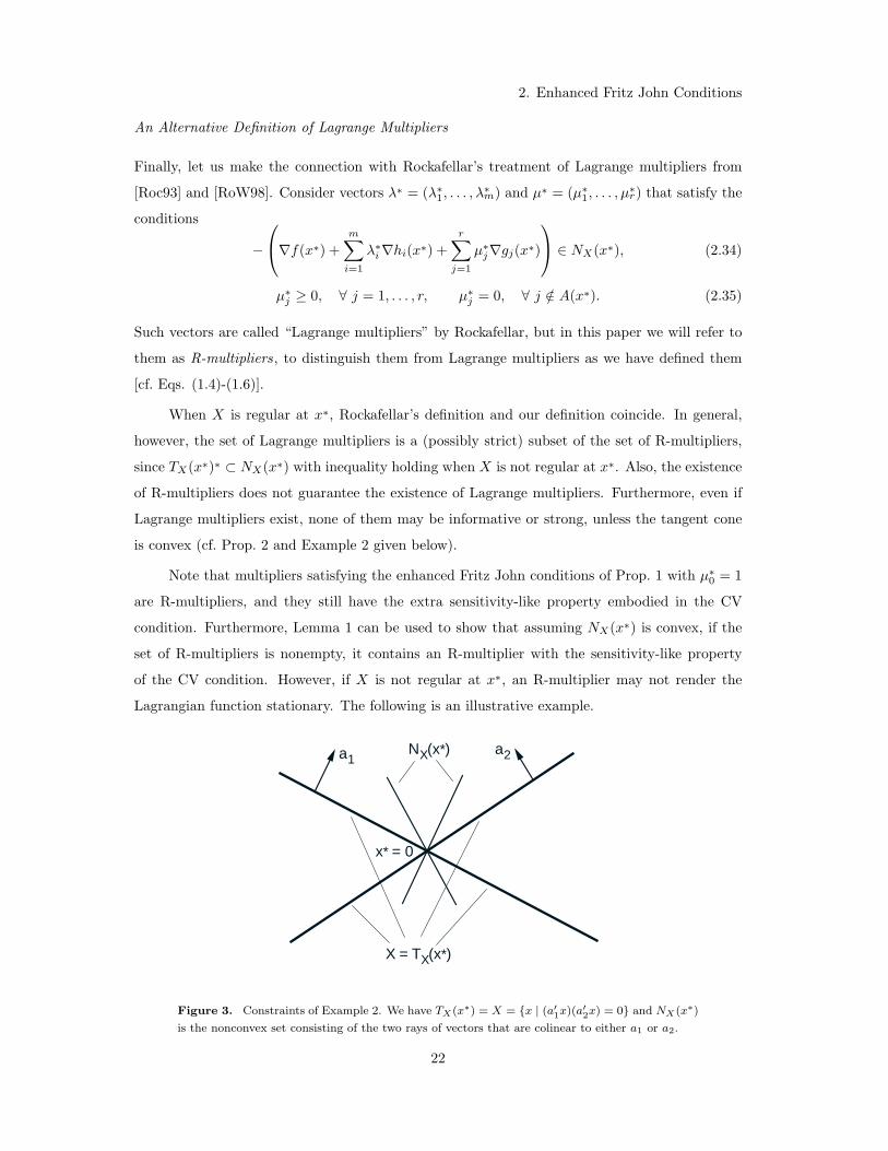
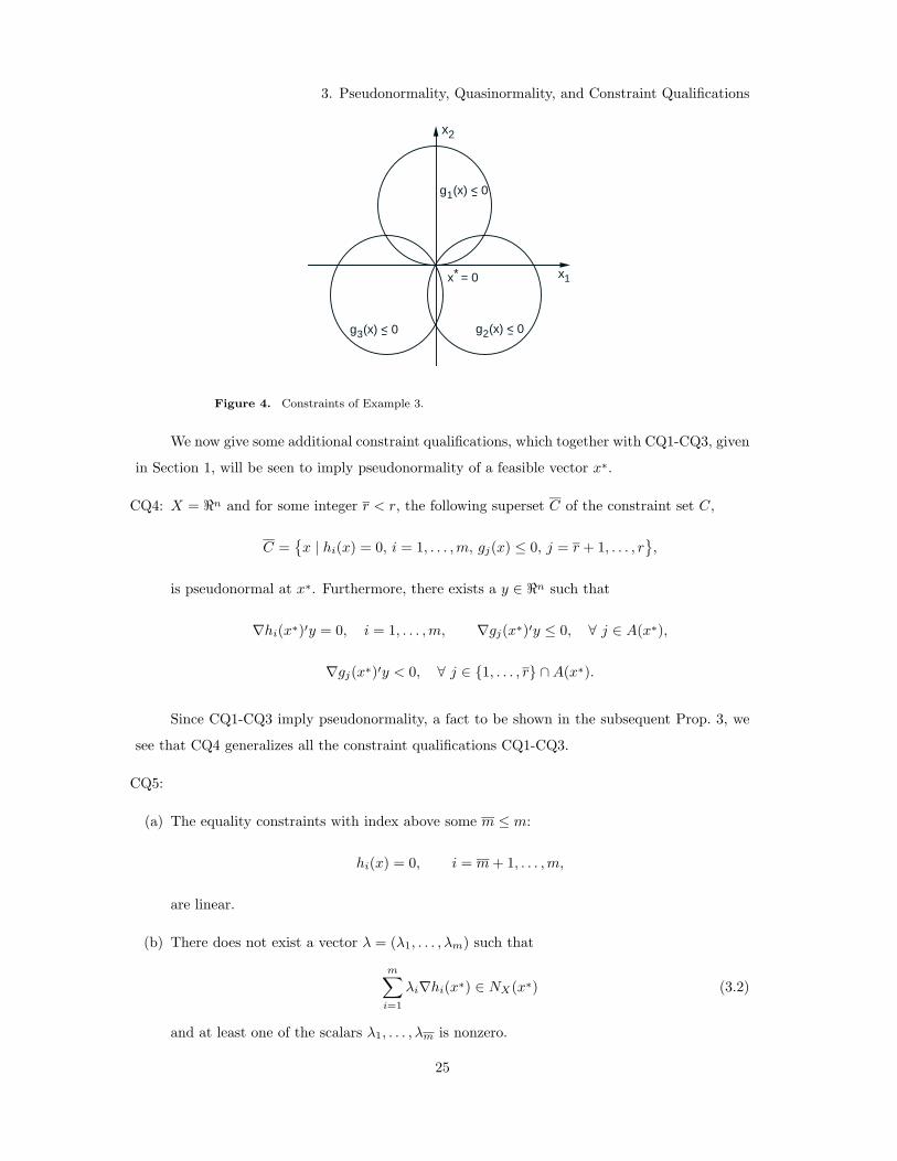
CQ4 : It is not possible that µj = 0 for all j ∈ {1, . . . , r}, since if this were so, the pseudonormality

assumption for C would be violated. Thus we have µj > 0 for some j ∈ {1, . . . , r} ∩ A(x∗). It

28


follows that for the vector y appearing in the statement of CQ4, we have∑r

j=1 µj∇gj(x∗)′y < 0,

so thatm∑

i=1

λi∇hi(x∗)′y +r∑

j=1

µj∇gj(x∗)′y < 0.

This contradicts the equation

m∑i=1


j=1

µj∇gj(x∗) = 0,

[cf. condition (i)].

CQ5 : We first show by contradiction that at least one of the λ1, . . . , λm and µj , j ∈ A(x∗) must

be nonzero. If this were not so, then by using a translation argument we may assume that x∗ is

the origin, and the linear constraints have the form a′ix = 0, i = m + 1, . . . , m. Using condition

(i) we have

−m∑

i=m+1

λiai ∈ NX(x∗). (3.5)

Let y be the interior point of NX(x∗)∗ that satisfies a′iy = 0 for all i = m + 1, . . . , m, and let S

be an open sphere centered at the origin such that y + d ∈ NX(x∗)∗ for all d ∈ S. We have from

Eq. (3.5),m∑

i=m+1

λia′id ≥ 0, ∀ d ∈ S,

from which we obtain∑m

i=m+1 λiai = 0. This contradicts condition (iii), which requires that

there exists some x ∈ S ∩ X such that∑m

i=m+1 λia′ix > 0.

Next we show by contradiction that we cannot have µj = 0 for all j. If this were so, by

condition (i) there must exist a nonzero vector λ = (λ1, . . . , λm) such that

−m∑

i=1

λi∇hi(x∗) ∈ NX(x∗). (3.6)

By what has been proved above, the multipliers λ1, . . . , λm of the nonlinear constraints cannot

be all zero, so Eq. (3.6) contradicts assumption (b) of CQ5.

Hence we must have µj > 0 for at least one j, and since µj ≥ 0 for all j with µj = 0 for

j /∈ A(x∗), we obtainm∑

i=1

λi∇hi(x∗)′y +r∑

j=1

µj∇gj(x∗)′y < 0,

for the vector y of NX(x∗)∗ that appears in assumption (d) of CQ5. Thus,

−

m∑

i=1


j=1

µj∇gj(x∗)

/∈

(NX(x∗)∗

)∗.

29


Since NX(x∗) ⊂(NX(x∗)∗

)∗, this contradicts condition (i). Q.E.D.

A consequence of Prop. 3 is that if any one of the constraint qualifications CQ1-CQ6 holds

and X is regular at x∗, by Prop. 1, the constraint set C admits informative Lagrange multipliers

at x∗. Without the regularity assumption on X, CQ5 and CQ6 similarly imply the admittance of

an R-multiplier vector. In the next section, we will also show similar implications regarding the

admittance of an exact penalty at x∗. To this end, we establish a relation between quasinormality

and a weaker version of pseudonormality.

Proposition 4: Let x∗ be a feasible vector of problem (1.1)-(1.2), and assume that the

normal cone NX(x∗) is convex. Then x∗ is quasinormal if and only if there are no scalars

λ1, . . . , λm, µ1, . . . , µr satisfying conditions (i)-(iii) of the definition of quasinormality together

with the following condition:

(iv′) {xk} converges to x∗ and for all k, λihi(xk) ≥ 0 for all i, µjgj(xk) ≥ 0 for all j, andm∑

i=1

λihi(xk) +r∑

j=1

µjgj(xk) > 0.

Proof: For simplicity we assume that all the constraints are inequalities that are active at

x∗. First we note that if there are no scalars µ1, . . . , µr with the properties described in the

proposition, then there are no scalars µ1, . . . , µr satisfying the more restrictive conditions (i)-(iv)

in the definition of quasinormality, so x∗ is not quasinormal.

To show the converse, suppose that there exist scalars µ1, . . . , µr satisfying conditions (i)-

(iii) of the definition of quasinormality together with condition (iv′), i.e., there exist scalars

µ1, . . . , µr such that:

(i) −(∑r

j=1 µj∇gj(x∗))∈ NX(x∗).

(ii) µj ≥ 0, for all j = 1, . . . , r.

(iii) {xk} converges to x∗ and for all k, gj(xk) ≥ 0 for all j, andr∑

j=1

µjgj(xk) > 0.

Condition (iii) implies that gj(xk) ≥ 0 for all j, and gj(xk) > 0 for some j such that µj > 0.

Without loss of generality, we can assume j = 1, so that we have g1(xk) > 0 for all k. Let

aj = ∇gj(x∗), j = 1, . . . , r. Then by appropriate normalization, we can assume that µ1 = 1, so

that

−

a1 +

r∑j=2

µjaj

∈ NX(x∗). (3.7)

30


If −a1 ∈ NX(x∗), the choice of scalars µ1 = 1 and µj = 0 for all j = 2, . . . , r, satisfies conditions

(i)-(iv) in the definition of quasinormality, hence x∗ is not quasinormal and we are done. Assume

that −a1 /∈ NX(x∗). The assumptions of Lemma 2 are satisfied, so it follows that there exist

scalars µ2, . . . , µr, not all 0, such that

−

a1 +

r∑j=2

µjaj

∈ NX(x∗), (3.8)

and a vector d ∈ NX(x∗)∗ with a′jd > 0, for all j = 2, . . . , r such that µj > 0. Thus

∇gj(x∗)′d > 0, ∀ j = 2, . . . , r with µj > 0, (3.9)

while by Eq. (3.8), the µj satisfy

−

∇g1(x∗) +

r∑j=2

µj∇gj(x∗)

∈ NX(x∗). (3.10)

Next, we show that the scalars µ1 = 1 and µ2, . . . , µr satisfy condition (iv) in the definition

of quasinormality, completing the proof. We use Thm. 6.26 and Thm. 6.28 of Rockafellar and

Wets [RoW98] to argue that for the vector d ∈ NX(x∗)∗ and the sequence xk constructed above,

there is a sequence dk ∈ TX(xk) such that dk → d. Since xk → x∗ and dk → d, by Eq. (3.9), we

obtain for all sufficiently large k,

∇gj(xk)′dk > 0, ∀ j = 2, . . . , r with µj > 0.

Since dk ∈ TX(xk), there exists a sequence {xkν} ⊂ X such that, for each k, we have xk

ν �= xk

for all ν and

xkν → xk,

xkν − xk

‖xkν − xk‖ → dk

‖dk‖ , as ν → ∞. (3.11)

For each j = 2, . . . , r such that µj > 0, we use Taylor’s theorem for the constraint function gj .

We have, for some vector sequence ξν converging to 0,

gj(xkν) = gj(xk) + ∇gj(xk)′(xk

ν − xk) + o(‖xkν − xk‖)

≥ ∇gj(xk)′(

dk

‖dk‖ + ξν

)‖xk

ν − xk‖ + o(‖xkν − xk‖)

= ‖xkν − xk‖

(∇gj(xk)′

dk

‖dk‖ + ∇gj(xk)′ξν +o(‖xk

ν − xk‖)‖xk

ν − xk‖

),

where the inequality above follows from Eq. (3.11) and the assumption that gj(xk) ≥ 0, for all j

and xk. It follows that for ν and k sufficiently large, there exists xkν ∈ X arbitrarily close to xk

such that gj(xkν) > 0, for all j = 2, . . . , r with µj > 0.

31

4. Pseudonormality and Admittance of an Exact Penalty

Since g1(xk) > 0 and g1 is a continuous function, we have that g1(x) > 0 for all x in some

neighborhood Vk of xk. Since xk → x∗ and xkν → xk for each k, by choosing ν and k sufficiently

large, we get gj(xkν) > 0 for j = 1 and each j = 2, . . . , r with µj > 0. This together with Eq.

(3.10), violates the quasinormality assumption of x∗, which completes the proof. Q.E.D.

The following example shows that convexity of NX(x∗) is an essential assumption for the

conclusion of Prop. 4.

Example 4

Here X is the subset of �2 given by

X ={x2 ≥ 0 |

((x1 + 1)2 + (x2 + 1)2 − 2

) ((x1 − 1)2 + (x2 + 1)2 − 2

)≤ 0

}(see Fig. 5). The normal cone NX(x∗) consists of the three rays shown in Fig. 5, and is not convex.

Let there be two inequality constraints with

g1(x) = −(x1 + 1)2 − (x2)2 + 1, g2(x) = −x2.

In order to have −∑

jµj∇gj(x

∗) ∈ NX(x∗), we must have µ1 > 0 and µ2 > 0. There is no x ∈ X

such that g2(x) > 0, so x∗ is quasinormal. However, for −2 ≤ x1 ≤ 0 and x2 = 0, we have x ∈ X,

g1(x) > 0, and g2(x) = 0. Hence x∗ does not satisfy the weak form of pseudonormality given in

Prop. 4.

x*=0

x2

x1

NX(x*)

XC∇g2(x*)

∇g1(x*)


4. PSEUDONORMALITY AND ADMITTANCE OF AN EXACT PENALTY

We will show that pseudonormality implies that the constraint set admits an exact penalty, which

in turn, together with regularity of X at x∗, implies that the constraint set admits Lagrange

32


multipliers. We first use the generalized Mangasarian-Fromovitz constraint qualification CQ5 to

obtain a necessary condition for a local minimum of the exact penalty function.

Proposition 5: Let x∗ be a local minimum of

Fc(x) = f(x) + c

m∑

i=1

|hi(x)| +r∑

j=1

g+j (x)

over X. Then there exist λ∗1, . . . , λ

∗m and µ∗

1, . . . , µ∗r such that

−

∇f(x∗) + c

m∑

i=1

λ∗i∇hi(x∗) +

r∑j=1

µ∗j∇gj(x∗)

∈ NX(x∗),

λ∗i = 1 if hi(x∗) > 0, λ∗

i = −1 if hi(x∗) < 0, λ∗i ∈ [−1, 1] if hi(x∗) = 0,

µ∗j = 1 if gj(x∗) > 0, µ∗

j = 0 if gj(x∗) < 0, µ∗j ∈ [0, 1] if gj(x∗) = 0.

Proof: The problem of minimizing Fc(x) over x ∈ X can be converted to the problem

minimize f(x) + c

m∑

i=1

wi +r∑

j=1

vj

subject to x ∈ X, hi(x) ≤ wi, −hi(x) ≤ wi, i = 1, . . . , m, gj(x) ≤ vj , 0 ≤ vj , j = 1, . . . , r,

which involves the auxiliary variables wi and vj . It can be seen that at the local minimum of this

problem that corresponds to x∗ the constraint qualification CQ5 is satisfied. Thus, by Prop. 3,

this local minimum is pseudonormal, and hence there exist multipliers satisfying the conditions of

Prop. 1 with µ∗0 = 1. With straightforward calculation, these conditions yield scalars λ∗

1, . . . , λ∗m

and µ∗1, . . . , µ

∗r , satisfying the desired conditions. Q.E.D.

Proposition 6: If x∗ is a feasible vector of problem (1.1)-(1.2), which is pseudonormal, the

constraint set admits an exact penalty at x∗.

Proof: Assume the contrary, i.e., that there exists a smooth f such that x∗ is a strict local

minimum of f over the constraint set C, while x∗ is not a local minimum over x ∈ X of the

function

Fk(x) = f(x) + k

m∑

i=1

|hi(x)| +r∑

j=1

g+j (x)

for all k = 1, 2, . . . Let ε > 0 be such that

f(x∗) < f(x), ∀ x ∈ C with x �= x∗ and ‖x − x∗‖ ≤ ε. (4.1)

33


Suppose that xk minimizes Fk(x) over the (compact) set of all x ∈ X satisfying ‖x − x∗‖ ≤ ε.

Then, since x∗ is not a local minimum of Fk over X, we must have that xk �= x∗, and that xk is

infeasible for problem (1.2), i.e.,

m∑i=1

|hi(xk)| +r∑

j=1

g+j (xk) > 0. (4.2)

We have

Fk(xk) = f(xk) + k

m∑

i=1

|hi(xk)| +r∑

j=1

g+j (xk)

≤ f(x∗), (4.3)

so it follows that hi(xk) → 0 for all i and g+j (xk) → 0 for all j. The sequence {xk} is bounded

and if x is any of its limit points, we have that x is feasible. From Eqs. (4.1) and (4.3) it then

follows that x = x∗. Thus {xk} converges to x∗ and we have ‖xk − x∗‖ < ε for all sufficiently

large k. This implies the following necessary condition for optimality of xk (cf. Prop. 5):

−

1

k∇f(xk) +

m∑i=1

λki ∇hi(xk) +

r∑j=1

µkj∇gj(xk)

∈ NX(xk), (4.4)

where

λki = 1 if hi(xk) > 0, λk

i = −1 if hi(xk) < 0, λki ∈ [−1, 1] if hi(xk) = 0,

µkj = 1 if gj(xk) > 0, µk

j = 0 if gj(xk) < 0, µkj ∈ [0, 1] if gj(xk) = 0.

In view of Eq. (4.2), we can find a subsequence {λk, µk}k∈K such that for some equality constraint

index i we have |λki | = 1 and hi(xk) �= 0 for all k ∈ K or for some inequality constraint index j

we have µkj = 1 and gj(xk) > 0 for all k ∈ K. Let (λ, µ) be a limit point of this subsequence. We

then have (λ, µ) �= (0, 0), µ ≥ 0. Using the closure of the mapping x �→ NX(x), Eq. (4.4) yields

−

m∑

i=1


j=1

µj∇gj(x∗)

∈ NX(x∗). (4.5)

Finally, for all k ∈ K, we have λki hi(xk) ≥ 0 for all i, µk

j gj(xk) ≥ 0 for all j, so that, for all

k ∈ K, λihi(xk) ≥ 0 for all i, µjgj(xk) ≥ 0 for all j. Since by construction of the subsequence

{λk, µk}k∈K, we have for some i and all k ∈ K, |λki | = 1 and hi(xk) �= 0, or for some j and all

k ∈ K, µkj = 1 and gj(xk) > 0, it follows that for all k ∈ K,

m∑i=1

λihi(xk) +r∑

j=1

µjgj(xk) > 0. (4.6)

Thus, Eqs. (4.5) and (4.6) violate the hypothesis that x∗ is pseudonormal. Q.E.D.

34


A cursory examination shows that the proof of Prop. 6 goes through if we substitute

pseudonormality with the weaker version of pseudonormality introduced in Prop. 4. Thus by

using also Prop. 4, we obtain the following:

Proposition 7: If x∗ is a feasible vector of problem (1.1)-(1.2), which is quasinormal, and the

normal cone NX(x∗) is convex, then the constraint set admits an exact penalty at x∗.

The following proposition establishes the connection between admittance of an exact penalty

and admittance of Lagrange multipliers. Regularity of X is an important condition for this

connection.

Proposition 8: Let x∗ be a feasible vector of problem (1.1)-(1.2), and let X be regular at x∗.

If the constraint set admits an exact penalty at x∗, it admits Lagrange multipliers at x∗.

Proof: Suppose that a given smooth function f(x) has a local minimum at x∗. Then the

function f(x) + ‖x− x∗‖2 has a strict local minimum at x∗. Since C admits an exact penalty at

x∗, there exist λ∗i and µ∗

j satisfying the conditions of Prop. 5. (The term ‖x − x∗‖2 in the cost

function is inconsequential, since its gradient at x∗ is 0.) In view of the regularity of X at x∗,

the λ∗i and µ∗

j are Lagrange multipliers. Q.E.D.

As an illustration of the above propositions, consider Example 3. Here, since x∗ is quasinor-

mal but not pseudonormal, Prop. 6 cannot be used. However, since X = �n and NX(x∗) = {0}is convex, Prop. 7 applies and shows that the constraint set admits an exact penalty at x∗. By

Prop. 8, since X is regular, the constraint set admits Lagrange multipliers at x∗. [This can also

be shown using the fact TC(x∗) = V (x∗) = {0}, which implies that X∗ is quasiregular.]

We will show in Example 5 in Section 7 that the converses of Props. 6 and 7 do not hold;

i.e., the admittance of an exact penalty function at a point x∗ does not imply pseudonormality

or quasinormality. Furthermore, we will also show in Example 8 that the regularity assumption

on X in Prop. 8 cannot be dispensed with. On the other hand, because Prop. 5 does not require

regularity of X, the proof of Prop. 8 can be used to establish that admittance of an exact penalty

implies the admittance of R-multipliers, as defined in Section 2. The relations shown thus far

are summarized in Fig. 6, which illustrates the unifying role of pseudonormality and quasinor-

mality. In this figure, unless indicated otherwise, the implications cannot be established in the

opposite direction without additional assumptions (Section 7 provides the necessary examples

and counterexamples).

35


Admittance of an ExactPenalty

Admittance of Informative andStrong Lagrange Multipliers

Quasiregularity

Quasinormality

Constraint QualificationsCQ1-CQ4

X = Rn

Pseudonormality

Constraint QualificationsCQ5, CQ6

X = Rn

Pseudonormality


Admittance of R-multipliers


Constraint QualificationsCQ5, CQ6

X = Rn and Regular


Quasinormality

Pseudonormality

Admittance of Informative andStrong Lagrange Multipliers


Figure 6. Relations between various conditions, which when satisfied at a local minimum x∗,

guarantee the admittance of an exact penalty and corresponding multipliers. In the case where

X is regular, the tangent and normal cones are convex. Hence, by Prop. 2(a), the admittance

of Lagrange multipliers implies the admittance of an informative Lagrange multiplier, while by

Prop. 7, quasinormality implies the admittance of an exact penalty.

36

5. Using the Extended Representation

5. USING THE EXTENDED REPRESENTATION

In practice, the set X can often be described in terms of smooth equality and inequality con-

straints:

X ={x | hi(x) = 0, i = m + 1, . . . ,m, gj(x) ≤ 0, j = r + 1, . . . , r

}.

Then the constraint set C can alternatively be described without an abstract set constraint, in

terms of all of the constraint functions

hi(x) = 0, i = 1, . . . ,m, gj(x) ≤ 0, j = 1, . . . , r.

We call this the extended representation of C, to contrast it with the representation (1.2), which

we call the original representation. Issues relating to exact penalty functions and Lagrange

multipliers can be investigated for the extended representation and results can be carried over to

the original representation by using the following proposition.

Proposition 9:

(a) If the constraint set admits Lagrange multipliers in the extended representation, it admits

Lagrange multipliers in the original representation.

(b) If the constraint set admits an exact penalty in the extended representation, it admits an

exact penalty in the original representation.

Proof: (a) The hypothesis implies that for every smooth cost function f for which x∗ is a local

minimum there exist scalars λ∗1, . . . , λ

∗m and µ∗

1, . . . , µ∗r satisfying

∇f(x∗) +m∑

i=1

λ∗i∇hi(x∗) +

r∑j=1

µ∗j∇gj(x∗) = 0, (5.1)

µ∗j ≥ 0, ∀ j = 0, 1, . . . , r,

µ∗j = 0, ∀ j /∈ A(x∗),

where

A(x∗) = {j | gj(x∗) = 0, j = 1, . . . , r}.

For y ∈ TX(x∗), we have ∇hi(x∗)′y = 0 for all i = m + 1, . . . ,m, and ∇gj(x∗)′y ≤ 0 for all

j = r + 1, . . . , r with j ∈ A(x∗). Hence Eq. (5.1) implies that

∇f(x∗) +

m∑i=1

λ∗i∇hi(x∗) +

r∑j=1

µ∗j∇gj(x∗)

′

y ≥ 0, ∀ y ∈ TX(x∗),

37

6. Extensions under Convexity Assumptions

and it follows that λ∗i , i = 1, . . . , m, and µ∗

j , j = 1, . . . , r, are Lagrange multipliers for the original

representation.

(b) Consider the exact penalty function for the extended representation:

F c(x) = f(x) + c

m∑

i=1

|hi(x)| +r∑

j=1

g+j (x)

.

We have Fc(x) = F c(x) for all x ∈ X. Hence if x∗ is an unconstrained local minimum of F c(x),

it is also a local minimum of Fc(x) over x ∈ X. Thus, for a given c > 0, if x∗ is both a strict local

minimum of f over C and an unconstrained local minimum of F c(x), it is also a local minimum

of Fc(x) over x ∈ X. Q.E.D.

Note that part (a) of the above proposition does not guarantee the existence of informative

Lagrange multipliers in the original representation, and indeed in Example 9 given in Section

7, there exist some informative Lagrange multipliers in the extended representation, but there

exists none in the original representation.

As an example where Prop. 9 is useful, consider the important special case where all con-

straints are linear and X is a polyhedron. Then the constraint set need not satisfy quasinormality,

as will be shown in Example 10 in Section 7. However, by Prop. 3, it satisfies quasinormality

in the extended representation, so using Prop. 9, it admits Lagrange multipliers and an exact

penalty at any feasible point in the original representation.

6. EXTENSIONS UNDER CONVEXITY ASSUMPTIONS

In this section, we extend the theory of preceding sections to the case where the functions f

and gj may be nondifferentiable, but are all instead assumed convex (a slightly more general

development is given in [BNO01], where each of the functions f and gj may be either smooth or

convex). We thus consider the problem

minimize f(x)

subject to x ∈ X, g(x) ≤ 0,(6.1)

where g(x) =(g1(x), . . . , gr(x)

)is the constraint function vector, and we assume that X is a

nonempty, closed, and convex set, and each of the functions f and gj is convex over �n. For

simplicity, we assume no equality constraints. The extension of the following analysis to the case

38


where there are linear equality constraints is straightforward: we simply replace each equality

constraint into two linear (and hence convex) inequality constraints.

For a convex function F , we use the notation ∂F (x) to denote the set of all subgradients of

F at x ∈ �n. To generalize the enhanced Fritz-John conditions under these assumptions, we use

the following classical condition for the problem of minimizing F (x) over X, where F is convex:

if x∗ is a local minimum of this problem and the tangent cone TX(x∗) is convex, then

0 ∈ ∂F (x∗) + TX(x∗)∗. (6.2)

By a nearly verbatim repetition of the proof of Prop. 1, while using this necessary condition

in place of −∇F k(xk) ∈ TX(xk)∗, together with the convexity assumptions on X, f , and gj , we

obtain the following extension of enhanced Fritz-John conditions:

Proposition 10: Consider problem (6.1), assuming that X is convex, and the functions f

and gj are convex over �n, and let x∗ be a global minimum. Then there exists a scalar µ∗0 and a

vector µ∗ = (µ∗1, . . . , µ

∗r), satisfying the following conditions:

(i) µ∗0f(x∗) = minx∈X

{µ∗

0f(x) + µ∗′g(x)}.

(ii) µ∗j ≥ 0 for all j = 0, 1, . . . , r.

(iii) µ∗0, µ

∗1, . . . , µ

∗r are not all equal to 0.

(iv) If the index set J = {j �= 0 | µ∗j > 0} is nonempty, there exists a sequence {xk} ⊂ X that

converges to x∗ and is such that for all k,

f(xk) < f(x∗), µ∗jgj(xk) > 0, ∀ j ∈ J,

gj(xk) = o

(minl∈J

gl(xk))

, ∀ j /∈ J.

The theory of the preceding sections can now be generalized using Prop. 10. We first extend

the definition of a Lagrange multiplier. If x∗ is a global minimum of problem (6.1), we say that

a vector µ∗ ≥ 0 is a Lagrange multiplier vector corresponding to f and x∗ if

f(x∗) = minx∈X

{f(x) + µ∗′g(x)

}, µ∗′g(x∗) = 0. (6.3)

Note here that since g(x∗) ≤ 0 and µ∗ ≥ 0, the condition µ∗′g(x∗) = 0 of Eq. (6.3) is equivalent

to the condition µ∗jgj(x∗) = 0 for all j, which is the CS condition.

Similarly, the definition of pseudonormality is extended as follows:

39


Definition 3: Consider problem (6.1), assuming that X is convex, and the functions f and

gj are convex over �n. A feasible vector x∗ is said to be pseudonormal if there exist no vector

µ = (µ1, . . . , µr) ≥ 0, and a sequence {xk} ⊂ X such that:

(i) 0 = µ′g(x∗) = infx∈X µ′g(x).

(ii) {xk} converges to x∗ and µ′g(xk) > 0 for all k.

If a global minimum x∗ is pseudonormal, by Prop. 10, there exists a Lagrange multiplier

vector, which also satisfies the extra CV condition (iv) of that proposition. Furthermore, the

analysis of Section 3 is easily extended to show that x∗ is pseudonormal under either one of the

following two criteria:

(a) Polyhedral criterion: X = �n and the functions gj are linear.

(b) Slater criterion: There exists a feasible vector x such that

gj(x) < 0, j = 1, . . . , r.

Thus, under either one of these criteria, a Lagrange multiplier vector is guaranteed to exist.

If X is a polyhedron (rather than X = �n) and the functions gj are linear, we can also prove

existence of at least one Lagrange multiplier, by combining the linearity criterion above with the

extended representation of the problem as in the preceding section. Also the Slater criterion can

be extended to the case where there are additional linear equality constraints. Then in addition

to the condition gj(x) < 0 for all j, for existence of a Lagrange multiplier, there should exist a

feasible vector in the relative interior of X.

Finally, let us provide a geometric interpretation of pseudonormality under convexity as-

sumptions. Consider the set

G = {g(x) | x ∈ X}

and hyperplanes that support this set at g(x∗). As Fig. 7 illustrates, pseudonormality of the

feasible point x∗ means that there is no hyperplane H with a normal µ ≥ 0 such that:

(1) H supports G at g(x∗) and passes through 0, i.e.,

H = {z | µ′z = µ′g(x∗) = 0}.

(2) g(x∗) can be approached by a sequence{g(xk)

}⊂ G ∩ int(H), where H is the upper

halfspace defined by the hyperplane H,

H = {z | µ′z ≥ 0}.

40


Figure 7 also indicates the type of constraint qualifications that guarantee pseudonormality.

The Slater condition can be rephrased to mean that the set G intersects the interior of the

nonpositive orthant. Clearly, if this is so, there cannot exist a hyperplane with a normal µ ≥ 0

that simultaneously supports G at g(x∗) and passes through 0. Similarly, if X = �n and the

gj are linear, the set G is an affine set, and if this is so, G is fully contained in the hyperplane

H and cannot intersect the interior of the upper halfspace H. Thus the polyhedral and Slater

criteria imply pseudonormality of all feasible points.

(a)

0

G = {g(x) | x ∈ X}

g(x*)

µ

x*: pseudonormal

H

(b)

0

G = {g(x) | x ∈ X}

g(x*)

µ

x*: pseudonormal

H

(c)

0

G = {g(x) | x ∈ X}

g(x*)

µ

x*: not pseudonormal

H

Figure 7. Geometric interpretation of pseudonormality. Consider the set

G = {g(x) | x ∈ X}

and hyperplanes that support this set at g(x∗). For feasibility, G should intersect the nonpositive

orthant {z | z ≤ 0}. The first condition [0 = µ′g(x∗) = infx∈X µ′g(x)] in the definition of

pseudonormality means that there is a hyperplane with normal µ, which simultaneously supports

G at g(x∗) and passes through 0 [note that, as illustrated in figure (a), this cannot happen if G

intersects the interior of the nonpositive orthant; cf. the Slater criterion]. The second condition

[{xk} converges to x∗ and µ′g(xk) > 0 for all k] means that g(x∗) can be approached by a sequence{g(xk)

}⊂ G ∩ int(H), where H is the upper halfspace defined by the hyperplane,

H = {z | µ′z ≥ 0};

[cf. figures (b) and (c)]. Pseudonormality of x∗ means that there is no µ ≥ 0 and {xk} ⊂ X

satisfying both of these conditions. If the Slater criterion holds, the first condition cannot be

satisfied. If the polyhedral criterion holds, the set G is an affine set and the second condition

cannot be satisfied (this depends critically on X = �n rather than X being a general polyhedron).

41

7. Examples and Counterexamples

7. EXAMPLES AND COUNTEREXAMPLES

In this section, we provide examples and counterexamples that clarify some of the earlier devel-

opments. In particular, we explore the relations between various conditions given in Fig. 6, and

we show (at least in the less obvious cases) that the one-directional arrows cannot be reversed in

the absence of additional assumptions.

Example 5

Here we show that even with X = �n, the admittance of an exact penalty does not imply pseudonor-

mality and quasinormality. Let C ={x ∈ �2 | g1(x) ≤ 0, g2(x) ≤ 0, h1(x) = 0

}, where

g1(x) = (x1 − 1)2 + x22 − 1,

g2(x) = (x1 + 1)2 + x22 − 1,

h1(x) = x2,

(see Fig. 8). The only feasible solution is x∗ = (0, 0) and the constraint gradients are given by

∇g1(x∗) = (−2, 0), ∇g2(x

∗) = (2, 0), ∇h1(x∗) = (0, 1).

Let µ1 = µ2 = 1 and λ = 0. With this choice of multipliers we have

µ1∇g1(x∗) + µ2∇g2(x

∗) + λ∇h1(x∗) = 0.

In addition it can be seen that arbitrarily close to x∗, there exists some x such that g1(x) > 0 and

g2(x) > 0 simultaneously. Thus x∗ is not quasinormal, and hence not pseudonormal.

g1(x) = 0

x* = 0

g2(x) = 0

∇g2(x*) ∇g1(x*)

∇h1(x*)

x2

x1

Figure 8. Constraints of Example 5. The only feasible point is x∗ = (0, 0).

On the other hand, the directional derivative of the function

P (x) = |h1(x)| +2∑

j=1

g+j (x)

42


at x∗ is positive in all directions. This is because the directional derivative of∑2

j=1g+

j (x) is

positive everywhere except in directions d1 = (0, 1) and d2 = (0,−1), and with the introduction

of the equality constraint, the function P (x) acquires a positive directional derivative in these

directions as well. By choosing a sufficiently large penalty parameter c, we can guarantee that x∗

is a local minimum of the function Fc(x). Hence the constraint set admits an exact penalty at x∗.

Example 6

Here we show that even with X = �n, the admittance of an exact penalty function does not imply

quasiregularity. Let C ={x ∈ �2 | g1(x) ≤ 0, g2(x) ≤ 0, g3(x) ≤ 0

}, where

g1(x) = −(x1 + 1)2 − (x2)2 + 1,

g2(x) = x21 + (x2 + 1)2 − 1,

g3(x) = −x2,

(see Fig. 9). The only feasible solution is x∗ = (0, 0) and the constraint gradients are given by

∇g1(x∗) = (−2, 0), ∇g2(x

∗) = (0, 2), ∇g3(x∗) = (0,−1).

At x∗ = (0, 0), the cone of first order feasible variations V (x∗) is equal to the nonnegative x1 axis

and strictly contains T (x∗), which is equal to x∗ only. Therefore x∗ is not a quasiregular point.

g1(x) = 0

x*=0=TX(x*)

g2(x) = 0

∇g2(x*)

∇g1(x*)

x2

x1

∇g3(x*)

V(x*)

Figure 9. Constraints of Example 6. The only feasible point is x∗ = (0, 0). The tangent

cone T (x∗) and the cone of first order feasible variations V (x∗) are also illustrated in the

figure.

However, it can be seen that the directional derivative of the function P (x) =∑3

j=1g+

j (x)

at x∗ is positive in all directions. This implies we can choose a sufficiently large penalty parameter

43


c, so that x∗ is a local minimum of the function Fc(x). The constraint set admits an exact penalty

function at x∗.

Example 7

Here we show that, when X = �n, the admittance of Lagrange multipliers with quasiregularity

(but not quasinormality) holding, does not imply the admittance of an exact penalty. Let C ={x ∈ �2 | g1(x) ≤ 0, g2(x) ≤ 0

}, where

g1(x) = x2,

g2(x) = x61 + x3

2.

At x∗ = (0, 0), the tangent cone is equal to the cone of first order feasible variations. Hence x∗

is a quasiregular point, which implies that the constraint set admits Lagrange multipliers at x∗.

However, it is not true that the constraint set admits an exact penalty function at x∗. For this

purpose, we consider the function f(x) = −x41 − x2, which is a smooth function with a strict local

minimum at x∗. By contrast, x∗ is not a local minimum of the function Fc(x) no matter how large

c is chosen. To illustrate this we define the function l(x1) = Fc(x1, 0) = −x41 + cx6

1, which has a

local maximum at x∗ for any c > 0. Hence the existence of Lagrange multipliers does not guarantee

the local exactness of the penalty function Fc(x).

Example 8

Here we show that if X is not regular, the admittance of an exact penalty does not imply the

admittance of Lagrange multipliers (although it does imply the admittance of R-multipliers). Con-

sider the set X ⊂ �2 depicted in Fig. 10, and let there be a single linear equality constraint

h(x) = x1 = 0. For x∗ = (0, 0), we have TX(x∗)∗ = {0}, while NX(x∗) consists of the two rays

shown in Fig. 10. Because ∇h(x∗) = (1, 0) /∈ NX(x∗), pseudonormality is satisfied, and hence

by Prop. 6, the constraint set admits an exact penalty at x∗. On the other hand for the cost

function f(x) = −x2, we have ∇f(x∗) + λ∇h(x∗) �= 0 for all λ, so there is no Lagrange multiplier.

The non-admittance of Lagrange multipliers can also be verified in this example by noting that

V (x∗)∗ + TX(x∗)∗ �= TC(x∗)∗.

Example 9

Here we show that there may exist informative Lagrange multipliers in the extended representation

of the constraint set, but not in the original representation. This suggests that the extended

representation of a constraint set cannot be used to infer the admittance of informative Lagrange

multipliers as opposed to other characteristics of the constraint set given by Prop. 9.

44


x*=0 ∇h(x*)

x2

x1

NX(x*)

X

C


Let the constraint set be represented in extended form without an abstract set constraint as

C ={x ∈ �2 | a′

1x ≤ 0, a′2x ≤ 0, (a′

1x)(a′2x) = 0

},

where a1 = (−1, 0) and a2 = (0,−1). Consider the vector x∗ = (0, 0). Here TC(x∗) consists

of the nonnegative coordinate axes, whereas V (x∗) is equal to the nonnegative orthant in the

extended representation, as shown in Fig. 11. Although x∗ is not a quasiregular point, we have

TC(x∗)∗ = V (x∗)∗, which (as mentioned in Section 1) is a necessary and sufficient condition for

the admittance of Lagrange multipliers at x∗ when X = �n. By Prop. 2, this implies that the

constraint set admits informative Lagrange multipliers in the extended representation.

V(x*)TC(x*)

TC(x*) ⊥ = V(x*)⊥

a1

a2

(a)

X = TX(x*)

TC(x*)

a1

a2

TC(x*) ⊥

(b)

-∇f(x*)

Figure 11. Constraints and relevant cones for different representations of the problem in

Example 9.

Now let the same constraint set be specified by the two linear constraint functions a′1x ≤ 0

45


and a′2x ≤ 0 together with the abstract constraint set

X = {x | (a′1x)(a′

2x) = 0}

Here TX(x∗) = X and TX(x∗)∗ = {0}. The normal cone NX(x∗) consists of the coordinate axes.

Since NX(x∗) �= TX(x∗)∗, X is not regular at x∗. Furthermore, TX(x∗) is not convex, so Prop.

2(a) cannot be used to guarantee the admittance of an informative Lagrange multiplier. For any f

for which x∗ is a local minimum, we must have −∇f(x∗) ∈ TC(x∗)∗ (see Fig. 11). The candidate

multipliers are determined from the requirement that

−(∇f(x∗) +

2∑j=1

µjaj

)∈ TX(x∗)∗ = {0},

which uniquely determines µ1 and µ2. If ∇f(x∗) lies in the interior of the positive orthant, we

need to have µ1 > 0 and µ2 > 0. However, there exists no x ∈ X that violates both constraints

a′1x ≤ 0 and a′

2x ≤ 0, so the multipliers do not qualify as informative. Thus, the constraint set

does not admit informative Lagrange multipliers in the original representation.

Example 10

Here we show that if the constraint set involves linear constraint functions and a polyhedral set X,

then x∗ need not be quasinormal (even though it admits Lagrange multipliers). Let C ={x ∈ X |

a′x ≤ 0, b′x ≤ 0}, where a = (1,−1), b = (−1,−1), and X =

{x ∈ �2 | a′x ≥ 0, b′x ≥ 0

}. The

constraint set is depicted in Fig. 12.

x*=0

x2

x1ab

X = TX(x*)

TX(x*)⊥

Figure 12. Constraints of Example 10. The only feasible point is x∗ = (0, 0). The tangent

cone TX(x∗) and its polar TX(x∗)∗ are shown in the figure.

46

References

The only feasible point is x∗ = (0, 0). By choosing µ = (1, 1), we get

− (a + b) ∈ TX(x∗)∗,

while in every neighborhood N of x∗ there is an x ∈ X ∩ N such that a′x > 0 and b′x > 0

simultaneously. Hence x∗ is not quasinormal. Note that this constraint set admits Lagrange

multipliers at x∗ = (0, 0) with respect to its extended representation (cf. Prop. 3), and hence

it admits Lagrange multipliers at x∗ = (0, 0) with respect to the original representation (cf. the

discussion at the end of Section 5).

Example 11

Here we show why in the definition of admittance of an exact penalty, it is necessary to restrict

attention to functions f with a strict local minimum at x∗. Consider the 2-dimensional constraint

set specified by

h(x) =x2

x21 + 1

= 0, x ∈ X = �2.

The feasible points are of the form x = (x1, 0) with x1 ∈ �, and at each of them the gradient

∇h(x∗) is nonzero, so CQ1 holds. If f(x) = x2, every feasible point is a local minimum, yet for

any c > 0, we have

infx∈�2

{x2 + c

|x2||x2

1 + 1|

}= −∞

(take x1 = x2 as x2 → −∞). Thus, the penalty function is not exact for any c > 0. It follows

that CQ1 would not imply the admittance of an exact penalty if we were to change the definition

of the latter to allow cost functions with nonstrict local minima. Note that for the cost function

f(x) = x2, it can be shown that the problem is not calm as per the definition of Clarke [Cla76],

[Cla83]. In particular, the primal function of this problem is given by

p(u) = infx2

x21+1

=u

x2 =

{u if u ≥ 0,

−∞ if u < 0,

and violates the definition of calmness as defined in [Cla83]. Thus CQ1 does not imply calmness,

illustrating a fundamental difference between the notions of calmness and of admittance of an exact

penalty.

REFERENCES

[AHU61] Arrow, K. J., Hurwicz, L., and Uzawa, H., 1961. “Constraint Qualifications in Maxi-

mization Problems,” Naval Research Logistics Quarterly, Vol. 8, pp. 175-191.

[Aba67] Abadie, J., 1967. “On the Kuhn-Tucker Theorem,” in Nonlinear Programming, Abadie,

J., (Ed.), North Holland, Amsterdam.

47

References

[AuF90] Aubin, J.-P., and Frankowska, H., Set-Valued Analysis, Birkhauser, Boston.

[BNO01] Bertsekas, D. P., with Nedic, A., and Ozdaglar, A. E., 2001. Lectures Notes on Con-

vexity, Duality, and Lagrange Multipliers, M.I.T., Cambridge, MA.

[BSS93] Bazaraa, M. S., Sherali, H. D., and Shetty, C. M., 1993. Nonlinear Programming Theory

and Algorithms, (2nd Ed.), Wiley, N. Y.

[BaG82] Bazaraa, M. S., and Goode, J. J., 1982. “Sufficient Conditions for a Globally Exact

Penalty Function without Convexity,” Math. Programming Stud., Vol. 19, pp. 1-15.

[Ber99] Bertsekas, D. P., “Nonlinear Programming: 2nd Edition,” Athena Scientific, Belmont,

MA, 1999.

[BoL00] Borwein, J. M., and Lewis, A. S., Convex Analysis and Nonlinear Optimization, Springer-

Verlag, N. Y.

[BoS00] Bonnans, J. F., and Shapiro, A., 2000. Perturbation Analysis of Optimization Problems,

Springer-Verlag, N. Y.

[Cla76] Clarke, F. H., 1976. Math. of Operations Reserach, Vol. 1 pp. 165-174.

[Cla83] Clarke, F. H., 1983. Optimization and Nonsmooth Analysis, Wiley, N. Y.

[Gau77] Gauvin, J., 1977. “A Necessary and Sufficient Condition to Have Bounded Multipliers

in Convex Programming,” Math. Programming., Vol. 12, pp. 136-138.

[GoT71] Gould, F. J., and Tolle, J., 1971. “A Necessary and Sufficient Condition for Constrained

Optimization,” SIAM J. Applied Math., Vol. 20, pp. 164-172.

[GoT72] Gould, F. J., and Tolle, J., 1972. “Geometry of Optimality Conditions and Constraint

Qualifications,” Math. Programming, Vol. 2, pp. 1-18.

[Gui69] Guignard, M., 1969. “Generalized Kuhn-Tucker Conditions for Mathematical Program-

ming Problems in a Banach Space,” SIAM J. on Control, Vol. 7, pp. 232-241.

[HaM79] Han, S. P., and Mangasarian, O. L., 1979. “Exact Penalty Functions in Nonlinear

Programming,” Math. Programming, Vol. 17, pp. 251-269.

[HiL93] Hiriart-Urruty, J.-B., and Lemarechal, C., 1993. Convex Analysis and Minimization

Algorithms, Vol. I, Springer-Verlag, Berlin and N. Y.

[Hes75] Hestenes, M. R., 1975. Optimization Theory: The Finite Dimensional Case, Wiley, N. Y.

[Joh48] John, F., 1948. “Extremum Problems with Inequalities as Subsidiary Conditions,” in

Studies and Essays: Courant Anniversary Volume, K. O. Friedrichs, Neugebauer, O. E., and

Stoker, J. J., (Eds.), Wiley-Interscience, N. Y., pp. 187-204.

48

References

[MaF67] Mangasarian, O. L., and Fromovitz, S., 1967. “The Fritz John Necessary Optimality

Conditions in the Presence of Equality and Inequality Constraints,” J. Math. Anal. and Appl.,

Vol. 17, pp. 37-47.

[McS73] McShane, E. J., 1973. “The Lagrange Multiplier Rule,” Amer. Mathematical Monthly,

Vol. 80, pp. 922-925.

[Mor76] Mordukhovich, B. S., 1976. “Maximum Principle in the Problem of Time Optimal Re-

sponse with Nonsmooth Constraints,” J. of Applied Mathematics and Mechanics, Vol. 40, pp.

960-969.

[Pet73] Peterson, D. W., 1973. “A Review of Constraint Qualifications in Finite-Dimensional

Spaces,” SIAM Review, Vol. 15, pp. 639-654.

[Pie69] Pietrzykowski, T., 1969. “An Exact Potential Method for Constrained Maxima,” SIAM

J. Numer. Anal., Vol. 6, pp. 294-304.

[RoW98] Rockafellar, R. T., and Wets, R. J.-B., 1998. Variational Analysis, Springer-Verlag,

Berlin.

[Roc70] Rockafellar, R. T., 1970. Convex Analysis, Princeton Univ. Press, Princeton, N. J.

[Roc73] Rockafellar, R. T., 1973. “A Dual Approach to Solving Nonlinear Programming Problems

by Unconstrained Minimization,” Math. Programming, Vol. 5, pp. 354-373.

[Roc93] Rockafellar, R. T., 1993. “Lagrange Multipliers and Optimality,” SIAM Review, Vol. 35,

pp. 183-238.

[Sla50] Slater, M., 1950. “Lagrange Multipliers Revisited: A Contribution to Non-Linear Pro-

gramming,” Cowles Commission Discussion paper, Math. 403.

[Zan67] Zangwill, W. I., 1967. “Nonlinear Programming via Penalty Functions,” Management

Sci., Vol. 13, pp. 344-358.

49

Date post:	05-Jul-2018
Category:	Documents
Upload:	danglien
View:	216 times
Download:	0 times

Pseudonormality and a Lagrange Multiplier Theory for ... 2000 Submitted for publication to JOTA...

Documents