Article history:Accepted 18 February 2014Available online 12 March 2014
Keywords:Fuzzy time seriesParticle swarm optimizationFuzzy c-meansForecastingDefine fuzzy relation
Fuzzy time series methods are effective techniques to forecast time series. Fuzzy time series methods are basedon fuzzy set theory. In the early years, classical fuzzy set operationswere used in the fuzzy time seriesmethods. Inrecent years, artificial intelligence techniques have been used in different stages of fuzzy time series methods. Inthis paper, a novel fuzzy time series method which is based on particle swarm optimization is proposed. A highorder fuzzy time series forecasting model is used in the proposed method. In the proposed method, determina-tion of fuzzy relations is performed by estimating the optimal fuzzy relation matrix. The performance of the pro-posed method is compared to some methods in the literature by using three real world time series. It is shownthat the proposed method has better performance than other methods in the literature.
Fuzzy time series methods have different approaches to uncertaintyfrom probabilistic statistical methods. Classical time series analysismethods are probabilistic methods, and they need some strict assump-tions. Moreover, probabilistic methods don't take into considerationfuzziness. However, some real life time series contain fuzziness. Becauseof this fact, various fuzzy time series methods were proposed in the lit-erature. Fuzzy time series methods do not need any assumptions likenormality and linearity.
Fuzzy time series methods were first defined in Song and Chissom(1993a). First definitions and methods were based on fuzzy set theoryand some fuzzy set operations. Song and Chissom (1993a) definedtwo different fuzzy time series types: time variant and time invariant.The first time invariant fuzzy time series method was proposed inSong and Chissom (1993b). There have been a lot of studies abouttime invariant fuzzy time series in the literature. But there have beena limited number of studies about time variant fuzzy time series.When fuzzy time series methods are examined, it can be said thatthey consist of three stages: fuzzification, determining fuzzy relationand defuzzification. Fuzzy time series methods are based on differentforecasting models. The forecasting models can be first order or highorder. When the first order models are used, it is assumed that fuzzytime series is caused by one order lagged fuzzy time series. Similarly,when nth order fuzzy time series forecasting model is used, fuzzytime series are caused by 1,2,…,n order lagged fuzzy time series.
In the literature, manymethods are used for determining fuzzy rela-tions. These methods are using fuzzy logic group relation tables, artifi-cial neural networks, fuzzy relation matrices obtained from somefuzzy set operations, particle swarm optimization and geneticalgorithms. Chen (1996, 2002), Lee et al. (2007, 2008), Duru et al.
(2010), Lee et al. (2013), Uslu et al. (2013), Bulut (2014) and Chenand Chen (2014) used fuzzy logic group relation tables. Aladag et al.(2009), Egrioglu et al. (2009a,b), Yolcu et al. (2013) and Aladag(2013) used some type of artificial neural networks. Song andChissom (1993b, 1994) used a fuzzy relation matrix obtained fromsome fuzzy set operations. Egrioglu (2012) used a fuzzy relation matrixobtained from a genetic algorithm and Aladag et al. (2012) used a fuzzyrelationmatrix obtained fromparticle swarmoptimization. Aladag et al.(2012) and Egrioglu (2012)methods are based on first order fuzzy timeseries forecastingmodels. The high order models are needed to forecastmany real life time series. Chen (2002), Lee et al. (2007, 2008), Kuo et al.(2009, 2010), Park et al. (2010), Chen and Chung (2006), Hsu et al.(2010), Egrioglu et al. (2009a,b, 2010), Aladag et al. (2009), Chen(2013), Qiu et al. (2013), and Jilani and Burney (2008) studies arebased on the high order fuzzy time series forecasting model. Somemethods which are used to determine fuzzy relations didn't take intoconsideration membership values of fuzzy sets. Song and Chissom(1993b), Yolcu et al. (2013), Yu and Huarng (2010), Egrioglu (2012)and Aladag et al. (2012) papers took into consideration membershipvalues of fuzzy sets.
In this study, a novel fuzzy time series method is proposed. The pro-posedmethod uses the fuzzy c-meanmethod in fuzzification stage, andthe particle swarm optimization method in the determining fuzzy rela-tion stage. The proposed method is based on the high order fuzzy timeseries forecasting model. The proposed method is an improved versionof the Aladag et al. (2012) method. Aladag et al. (2012) was based onthe first order fuzzy time series forecasting model as distinct from theproposed method. Particle swarm optimization is summarized in thesecond section of this paper. In the third section, the particulars of theproposedmethodare given. The application results are given in the fourthsection. The results are discussed in the last section of the paper.
634 E. Egrioglu / Economic Modelling 38 (2014) 633–639
2. Particle swarm optimization
Particle swarm optimization, which is an artificial intelligence tech-nique, was firstly proposed by Kenedy and Eberhart (1995). There havebeen different versions of particle swarm optimization in the literature.Shi and Eberhart (1999) used time varying inertia weight and Ma et al.(2006) used time varying acceleration coefficients in their algorithm. Analgorithmwhich uses time varying inertiaweight and a time varying ac-celeration coefficient is given below. We called this algorithmmodifiedparticle swarm optimization. This algorithm was firstly used in Aladaget al. (2012).
Algorithm 1. The modified particle swarm optimization
Step 1. Positions of each kth (k = 1,2, …, pn) particle's positions arerandomly determined and kept in a Xk given as follows:
Xk ¼ xk ;1; xk ;2;…; xk ;dn o
; k ¼ 1;2;…; pn ð1Þ
where xk,i (i = 1,2,…,d) represents ith position of kth particle.pn and d represent the number of particles in a swarm and po-sitions in a particle, respectively.
Step 2. Velocities are randomly determined and stored in a vector Vk
given below.
Vk ¼ vk;1; vk;2;…; vk;dn o
; k ¼ 1;2;…;pn: ð2Þ
Step 3. According to the evaluation function, Pbest and Gbest particlesgiven in Eqs. (1) and (2), respectively, are determined.
Pbestk ¼ pk;1;pk;2;…;pk;d� �
; k ¼ 1;2;…;pn ð3Þ
Gbest ¼ pg;1;pg;2;…;pg;d� �
ð4Þ
where Pbestk is a vector stores the positions corresponding tothe kth particle's best individual performance, and Gbest repre-sents the best particle, which has the best evaluation functionvalue found so far.
Fig. 1. Flow chart of the
Step 4. Let c1 and c2 represent cognitive and social coefficients, respec-tively, and w is the inertia parameter. Let (c1i, c1f), (c2i, c2f), and(w1,w2) be the intervals which include possible values for c1, c2andw, respectively. In each iteration, these parameters are cal-culated by using the formulas given in Eqs. (5), (6) and (7).
c1 ¼ c1 f−c1i� � t
maxtþ c1i ð5Þ
c2 ¼ c2 f−c2i� �maxt−t
maxtþ c2i ð6Þ
w ¼ w2−w1ð Þmaxt−tmaxt
þw1 ð7Þ
where maxt and t represent the maximum iteration numberand the current iteration number, respectively.
Step 5. Values of velocities and positions are updated by using the for-mulas given in Eqs. (8) and (9), respectively.
vtþ1i; j ¼ w� vti; j þ c1 � rand1 � pi; j−xti; j
� �þ c2 � rand2 � pg; j−xti; j
� �h i
ð8Þ
xtþ1i; j ¼ xti; j þ vtþ1
i; j ð9Þ
where rand1 and rand2 are generated random values from theinterval [0,1].
Step 6. Steps 3 to 5 are repeated until a predetermined maximum iter-ation number (maxt) is reached.
3. The proposed method
There have been a lot of studies about fuzzy time series methods inthe literature. The most important differences in fuzzy time seriesmethods from classical methods aremembership values and the advan-tages of membership values. Although the defuzzification process isperformed in the fuzzy time series methods, obtaining fuzzy forecasts
is still a good advantage because ofmembership values. In the literature,some studies didn't take into consideration these membership values inthe determination of fuzzy relation stage. Aladag et al. (2012) proposeda fuzzy time series method which is based on particle swarm optimiza-tion. The Aladag et al. (2012) method used the first order fuzzy time se-ries forecasting method. Better quality forecasts can be obtained fromhigh order models instead of first order models. The high order fuzzytime series forecasting model is defined as below.
Definition. Let F(t) be a time invariant fuzzy time series. If F(t) is causedby F(t− 1), F(t− 2),…, and F(t− n) then this fuzzy logical relationshipis represented by
F t−nð Þ;…; F t−2ð Þ; F t−1ð Þ→F tð Þ ð10Þ
and it is called the nth order fuzzy time series forecasting model.To obtain forecasts from a high order model (10) can be used in in-
tersection operations. After R fuzzy relation matrix is obtained, fuzzyforecasts can be calculated by using Eq. (11).
F tð Þ ¼ F t−nð Þ∩…∩F t−2ð Þ∩F t−1ð Þ∘Rð Þ ð11Þ
where “°” is max–min composition. R matrix was obtained by usingmax–min compositions and union operations in Song and Chissom(1993b). These operations were very complex and time consuming inSong and Chissom (1993b).
Model (10) is used in the proposed novel fuzzy time series forecast-ing method. The novel method is an improved version to high ordermodels of Aladag et al. (2012). The proposed method is using thefuzzy c-mean method that was proposed in Bezdek (1981) in thefuzzification stage, and the particle swarm optimization method in thedetermining fuzzy relation stage. Some advantages of the proposedmethod are listed below:
• Because of using fuzzy c-means in fuzzification stage, there is no needfor subjective decisions like determining interval length.
• The proposed method takes into consideration membership values.• Because R relation matrix is obtained from particle swarm optimiza-tion, there is no necessity for complex and time consuming matrixoperations.
• Because the proposed method is based on the high order fuzzy timeseries forecasting model, the better quality forecasts can be obtainfrom the proposed method for real life time series.
Fig. 3. The sequence chart of IMKB data.
The proposedmethod is given in Algorithm 2 and a flow chart of theproposed method is given in Fig. 1.
Algorithm 2.
Step 1. The parameters of the proposed method are determined. Theseparameters are:
pn: Particle number of swarm[c1i, c1f]: Cognitive coefficient interval[c2i, c2f]: Social coefficient intervalmaxt:Maximum iteration numberfsn: Number of fuzzy setntest: Observation number of testn: Model order.The root ofmean square error (RMSE) is used as a fitness function in theproposed method. RMSE is calculated according to Eq. (12).
where yt, yt, and n represent crisp time series, defuzzified forecasts, andthe number of forecasts, respectively.Step 2. The fuzzy c-meanmethod is applied to the training data of time
series. The cluster centers of fsn fuzzy sets Lr (r= 1,2,…,fsn) andmembership values of training data observations are obtainedby the fuzzy c-mean method. The fuzzy sets are redesigned ac-cording to the ascending ordered centers. The membershipvalues of test data observations are obtained from cluster cen-ters which were determined for training data by fuzzy c-mean. Fuzzy c-mean method is iteratively applied according tothe Bezdek (1981) procedure. First, the initial cluster centersare simulated by the interval on which time series is defined.The memberships are calculated according to Eq. (14).Eqs. (13) and (14) are consecutively used.
vi ¼
Xnj¼1
uβij x j
Xnj¼1
uβij
ð13Þ
uij ¼1
Xfsnk¼1
d xj; vi� �
d xj; vk� �
0@
1A
2= β−1ð Þð14Þ
where β is fuzziness indices and d(.) is Euclidean distance, x1, x2,…, xn are observations of training data and uij is membershipvalue of xj to ith fuzzy set. At the end of the FCM application pro-cesses, cluster centers vi(i = 1, 2, …, c) and membership valuesof training data observations to all fuzzy sets (uij, i = 1, 2, …, c;j = 1, 2, …, n) are obtained. The cluster centers are sorted intoan ascending order and the membership values are arrangedby the sort of orders.
Step 3. Generate a random initial positions and velocities.In the proposed method, positions are generated by uniformdistribution with (0,1) parameters. Velocities are generatedby uniform distribution with (−1,1). There are pn particles
a Distribution based method.b Average based method.
636 E. Egrioglu / Economic Modelling 38 (2014) 633–639
and velocities in the swarm. One particle has d positions. Inthe proposed method, positions of a particle are elements ofR fuzzy relation matrix. R fuzzy relation matrix has fsn col-umns and fsn rows and d= fsn × fsn. Each fuzzy relation ma-trix (Ri, i = 1, 2, …, pn) is obtained from each particle.
Step 4. Fitness (RMSE) values of the particles are calculated. In theproposed method, Steps 4.1 and 4.4 are applied to calculatethe RMSE value for each particle.
Step 4.1. Ri fuzzy relation matrix is constituted from particle posi-tions. The ith particle is shown in Fig. 2.Then R matrix is designed from ith particle as below:
Step 4.2. Fuzzy forecasts for training data are calculated byusing Eq. (11). For example, let model order be 2,fsn = 3, F(t− 1) = [0.7 0.3 0], F(t− 2) = [0.5 0.5 0] and
R ¼1 0:5 0:50:1 0 10:1 0 1
24
35:
Then, fuzzy forecast for t time is calculated as below:
F tð Þ ¼ F t−2ð Þ∩F t−1ð Þ�R� �F t−2ð Þ∩F t−1ð Þ ¼ min 0:7;0:5ð Þ; min 0:3;0:5ð Þ; min 0;0ð Þ½ � ¼ 0:5 0:3 0½ �
F tð Þ ¼ 0:5;0:3;0½ ��1 0:5 0:50:1 0 10:1 0 1
24
35
6000
6500
7000
7500
Fig. 4. The sequence chart of TAIFEX data.
¼ max min 0:5;1ð Þ; min 0:3;0:1ð Þ; min 0;0:1ð Þð Þ
�max min 0:5;0:5ð Þ; min 0:3;0ð Þ; min 0;0ð Þð Þmax min 0:5;1ð Þ; min 0:3;0:1ð Þ; min 0;0:1ð Þð Þ�
Step 4.3. Defuzzified forecasts are obtained. The ordered clustercenters of fuzzy sets and membership values of fuzzyforecasts are used for the defuzzification stage.
• If themembership values of the fuzzy forecast have only onemax-imum, then take the center value of this set as the defuzzified fore-casted value.
• If membership values of fuzzy forecast have two ormore consecu-tive maximums, then select the arithmetic mean of the centers ofthe corresponding clusters as the defuzzified forecasted value.
• Otherwise, standardize the fuzzy output and use the center of thefuzzy sets as the forecasted value.
Step 4.4. RMSE value is calculated according to Eq. (12).Step 5. According to RMSE, the Pbest and Gbest particles which are
given in Eqs. (3) and (4), respectively, are determined.Step 6. Update cognitive coefficient c1, social coefficient c2, and the in-
ertia parameter w at each iteration by using the formulas (5),(6) and (7), respectively.
Step 7. New velocities and positions of the particles are calculated byusing the formulas given in Eqs. (8) and (9).
Step 8. Repeat Step 4 to Step 8 until maximum iteration bound (maxt)is reached.
Step 9. Gbest gives optimal fuzzy relation matrix (Roptimal). Theforecasts and RMSE value for test data are calculated byusing Roptimal and applying Steps 4.2 and 4.4.
4. The application
In the literature, there are many studies about stock exchange fore-casting.Wei (2013) and Cheng et al. (2013) proposed newhybrid ANFIS(adaptive network fuzzy inference system) methods to forecast TAIEXdata. Cheng and Wei (2014) proposed a hybrid method to forecastTAIEX. In this study, the proposed method's performance is comparedwith some methods by using three different sets of the stock indextime series. The application results are given in the subsections.
4.1. IMKB application
The first time series is the data of Index 100 for the stocks and bondsexchangemarket of Istanbul (IMKB). Observations of IMKB are obtaineddaily between 03/October/2008 and 31/December/2008. A sequencechart of IMKB is given in Fig. 3. The time series has 59 observations.
Table 2Forecasting results for TAIFEX data set.
Date Test set Lee et al. (2007) Lee et al. (2008) Aladag et al. (2009) Hsu et al. (2010) Aladag (2013) Aladag et al. (2012) Proposed method
The first 52 and the last 7 observations are used as the training and thetest sets, respectively.
In Yolcu et al. (2013), IMKB data set was forecasted by Song andChissom (1993b), Chen (1996), and Huarng (2001) distribution and av-erage based methods, and Huarng and Yu (2006), and Cheng et al.(2008) methods. The forecasts and RMSE, mean absolute percentageerror (MAPE) and mean absolute error (MAE) values of these methodsare given in Table 1. MAPE and MAE values are calculated by using Eqs.(15)–(16).
MAPE ¼ 1n
Xnt¼1
yt−ytyt
�������� ð15Þ
MAE ¼ 1n
Xnt¼1
yt−ytj j: ð16Þ
The best forecasts are obtained from thesemethods in the followingsituations: In Song and Chissom (1993b), the number of fuzzy sets is 12;in Chen (1996), length of interval is 1200; in Huarng and Yu (2006)ratio based method, ratio sample percentile is 0.5; in Cheng et al.(2008), the number of fuzzy sets is 5; in Yolcu et al. (2013) method,the number of fuzzy sets is 11 and the number of hidden layer neuronsis 5. In the Huarng (2001) distribution based method, length of intervalis 800; in average basedmethod, length of interval is 200.Moreover, the
5100
5600
6100
6600
7100
7600
TAIEX
Fig. 5. The sequence graph of TAIEX Data.
best result obtained from the proposedmethod is given in Table 1. Iffivefuzzy sets and secondordermodel are used in the proposedmethod, thebest forecast result can be obtained from IMKB data set. In this situation,it obtained the optimal R matrix given below.
If Table 1 is examined, it is clear that the proposed method is betterthan the others according to RMSE and MAPE criteria.
4.2. Taiwan future exchange application
Secondly, the proposed method is applied to Taiwan future ex-change (TAIFEX) data whose observations are between 03.08.1998and 30.09.1998. The time series has 47 observations. The first 31 andthe last 16 observations are used as the training and the test sets, re-spectively. The graph of TAIFEX is given in Fig. 4.
TAIFEX data is forecasted by the proposed method. TAIFEX data isalso forecasted by using methods proposed by Lee et al. (2007, 2008),Aladag et al. (2009), Hsu et al. (2010), Aladag (2013) and Aladag et al.(2012). The forecast results produced by the methods proposed inAladag et al. (2009), Hsu et al. (2010), Aladag (2013) and Aladag et al.(2012) were taken from corresponding papers. When the proposed
Table 3The results obtained from all methods.
Method RMSE
Song and Chissom (1993b) 77.86Chen (1996) 77.18Chen (2002) 71.98Huarng and Yu (2006) 63.57Huarng et al. (2007) 72.35Yu and Huarng (2008) 67.00Aladag et al. (2009) 69.80Chen and Chen (2011) 57.30Proposed method 51.14
638 E. Egrioglu / Economic Modelling 38 (2014) 633–639
method is applied to TAIFEX data, the best forecasts are obtained fromsecond order model and five fuzzy sets. All forecasted results are givenin Table 2.
4.3. Taiwan Stock Exchange CapitalizationWeighted Stock Index Application
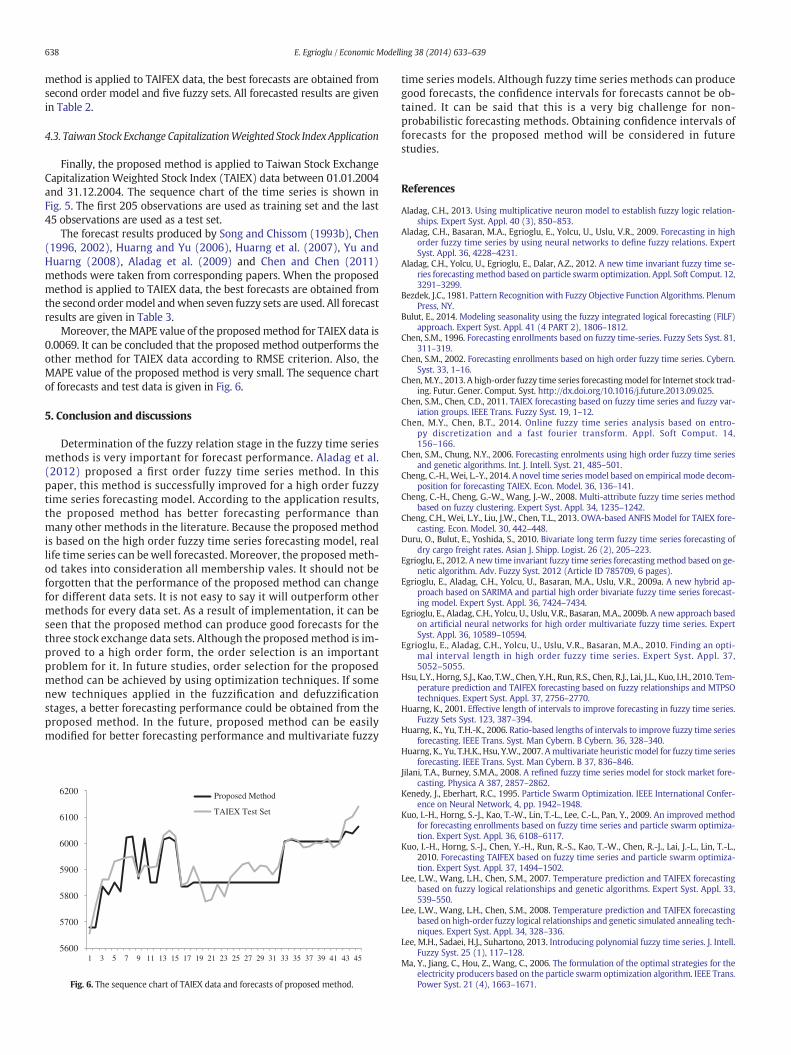
Finally, the proposed method is applied to Taiwan Stock ExchangeCapitalization Weighted Stock Index (TAIEX) data between 01.01.2004and 31.12.2004. The sequence chart of the time series is shown inFig. 5. The first 205 observations are used as training set and the last45 observations are used as a test set.
The forecast results produced by Song and Chissom (1993b), Chen(1996, 2002), Huarng and Yu (2006), Huarng et al. (2007), Yu andHuarng (2008), Aladag et al. (2009) and Chen and Chen (2011)methods were taken from corresponding papers. When the proposedmethod is applied to TAIEX data, the best forecasts are obtained fromthe second ordermodel andwhen seven fuzzy sets are used. All forecastresults are given in Table 3.
Moreover, theMAPE value of the proposedmethod for TAIEX data is0.0069. It can be concluded that the proposed method outperforms theother method for TAIEX data according to RMSE criterion. Also, theMAPE value of the proposed method is very small. The sequence chartof forecasts and test data is given in Fig. 6.
5. Conclusion and discussions
Determination of the fuzzy relation stage in the fuzzy time seriesmethods is very important for forecast performance. Aladag et al.(2012) proposed a first order fuzzy time series method. In thispaper, this method is successfully improved for a high order fuzzytime series forecasting model. According to the application results,the proposed method has better forecasting performance thanmany other methods in the literature. Because the proposed methodis based on the high order fuzzy time series forecasting model, reallife time series can bewell forecasted. Moreover, the proposedmeth-od takes into consideration all membership vales. It should not beforgotten that the performance of the proposed method can changefor different data sets. It is not easy to say it will outperform othermethods for every data set. As a result of implementation, it can beseen that the proposed method can produce good forecasts for thethree stock exchange data sets. Although the proposedmethod is im-proved to a high order form, the order selection is an importantproblem for it. In future studies, order selection for the proposedmethod can be achieved by using optimization techniques. If somenew techniques applied in the fuzzification and defuzzificationstages, a better forecasting performance could be obtained from theproposed method. In the future, proposed method can be easilymodified for better forecasting performance and multivariate fuzzy
Fig. 6. The sequence chart of TAIEX data and forecasts of proposed method.
time series models. Although fuzzy time series methods can producegood forecasts, the confidence intervals for forecasts cannot be ob-tained. It can be said that this is a very big challenge for non-probabilistic forecasting methods. Obtaining confidence intervals offorecasts for the proposed method will be considered in futurestudies.
References
Aladag, C.H., 2013. Using multiplicative neuron model to establish fuzzy logic relation-ships. Expert Syst. Appl. 40 (3), 850–853.
Aladag, C.H., Basaran, M.A., Egrioglu, E., Yolcu, U., Uslu, V.R., 2009. Forecasting in highorder fuzzy time series by using neural networks to define fuzzy relations. ExpertSyst. Appl. 36, 4228–4231.
Aladag, C.H., Yolcu, U., Egrioglu, E., Dalar, A.Z., 2012. A new time invariant fuzzy time se-ries forecasting method based on particle swarm optimization. Appl. Soft Comput. 12,3291–3299.
Bezdek, J.C., 1981. Pattern Recognition with Fuzzy Objective Function Algorithms. PlenumPress, NY.
Bulut, E., 2014. Modeling seasonality using the fuzzy integrated logical forecasting (FILF)approach. Expert Syst. Appl. 41 (4 PART 2), 1806–1812.
Chen, S.M., 1996. Forecasting enrollments based on fuzzy time-series. Fuzzy Sets Syst. 81,311–319.
Chen, S.M., 2002. Forecasting enrollments based on high order fuzzy time series. Cybern.Syst. 33, 1–16.
Chen, M.Y., 2013. A high-order fuzzy time series forecastingmodel for Internet stock trad-ing. Futur. Gener. Comput. Syst. http://dx.doi.org/10.1016/j.future.2013.09.025.
Chen, S.M., Chen, C.D., 2011. TAIEX forecasting based on fuzzy time series and fuzzy var-iation groups. IEEE Trans. Fuzzy Syst. 19, 1–12.
Chen, M.Y., Chen, B.T., 2014. Online fuzzy time series analysis based on entro-py discretization and a fast fourier transform. Appl. Soft Comput. 14,156–166.
Chen, S.M., Chung, N.Y., 2006. Forecasting enrolments using high order fuzzy time seriesand genetic algorithms. Int. J. Intell. Syst. 21, 485–501.
Cheng, C.-H.,Wei, L.-Y., 2014. A novel time series model based on empirical mode decom-position for forecasting TAIEX. Econ. Model. 36, 136–141.
Cheng, C.-H., Cheng, G.-W., Wang, J.-W., 2008. Multi-attribute fuzzy time series methodbased on fuzzy clustering. Expert Syst. Appl. 34, 1235–1242.
Cheng, C.H., Wei, L.Y., Liu, J.W., Chen, T.L., 2013. OWA-based ANFIS Model for TAIEX fore-casting. Econ. Model. 30, 442–448.
Duru, O., Bulut, E., Yoshida, S., 2010. Bivariate long term fuzzy time series forecasting ofdry cargo freight rates. Asian J. Shipp. Logist. 26 (2), 205–223.
Egrioglu, E., 2012. A new time invariant fuzzy time series forecastingmethod based on ge-netic algorithm. Adv. Fuzzy Syst. 2012 (Article ID 785709, 6 pages).
Egrioglu, E., Aladag, C.H., Yolcu, U., Basaran, M.A., Uslu, V.R., 2009a. A new hybrid ap-proach based on SARIMA and partial high order bivariate fuzzy time series forecast-ing model. Expert Syst. Appl. 36, 7424–7434.
Egrioglu, E., Aladag, C.H., Yolcu, U., Uslu, V.R., Basaran, M.A., 2009b. A new approach basedon artificial neural networks for high order multivariate fuzzy time series. ExpertSyst. Appl. 36, 10589–10594.
Egrioglu, E., Aladag, C.H., Yolcu, U., Uslu, V.R., Basaran, M.A., 2010. Finding an opti-mal interval length in high order fuzzy time series. Expert Syst. Appl. 37,5052–5055.
Hsu, L.Y., Horng, S.J., Kao, T.W., Chen, Y.H., Run, R.S., Chen, R.J., Lai, J.L., Kuo, I.H., 2010. Tem-perature prediction and TAIFEX forecasting based on fuzzy relationships and MTPSOtechniques. Expert Syst. Appl. 37, 2756–2770.
Huarng, K., 2001. Effective length of intervals to improve forecasting in fuzzy time series.Fuzzy Sets Syst. 123, 387–394.
Huarng, K., Yu, T.H.-K., 2006. Ratio-based lengths of intervals to improve fuzzy time seriesforecasting. IEEE Trans. Syst. Man Cybern. B Cybern. 36, 328–340.
Huarng, K., Yu, T.H.K., Hsu, Y.W., 2007. Amultivariate heuristicmodel for fuzzy time seriesforecasting. IEEE Trans. Syst. Man Cybern. B 37, 836–846.
Jilani, T.A., Burney, S.M.A., 2008. A refined fuzzy time series model for stock market fore-casting. Physica A 387, 2857–2862.
Kenedy, J., Eberhart, R.C., 1995. Particle Swarm Optimization. IEEE International Confer-ence on Neural Network, 4, pp. 1942–1948.
Kuo, I.-H., Horng, S.-J., Kao, T.-W., Lin, T.-L., Lee, C.-L., Pan, Y., 2009. An improved methodfor forecasting enrollments based on fuzzy time series and particle swarm optimiza-tion. Expert Syst. Appl. 36, 6108–6117.
Kuo, I.-H., Horng, S.-J., Chen, Y.-H., Run, R.-S., Kao, T.-W., Chen, R.-J., Lai, J.-L., Lin, T.-L.,2010. Forecasting TAIFEX based on fuzzy time series and particle swarm optimiza-tion. Expert Syst. Appl. 37, 1494–1502.
Lee, L.W., Wang, L.H., Chen, S.M., 2007. Temperature prediction and TAIFEX forecastingbased on fuzzy logical relationships and genetic algorithms. Expert Syst. Appl. 33,539–550.
Lee, L.W., Wang, L.H., Chen, S.M., 2008. Temperature prediction and TAIFEX forecastingbased on high-order fuzzy logical relationships and genetic simulated annealing tech-niques. Expert Syst. Appl. 34, 328–336.
Lee, M.H., Sadaei, H.J., Suhartono, 2013. Introducing polynomial fuzzy time series. J. Intell.Fuzzy Syst. 25 (1), 117–128.
Ma, Y., Jiang, C., Hou, Z., Wang, C., 2006. The formulation of the optimal strategies for theelectricity producers based on the particle swarm optimization algorithm. IEEE Trans.Power Syst. 21 (4), 1663–1671.
Park, J.-I., Lee, D.-J., Song, C.-K., Chun, M.-G., 2010. TAIFEX and KOSPI 200 forecastingbased on two factors high order fuzzy time series and particle swarm optimization.Expert Syst. Appl. 37, 959–967.
Qiu, W., Liu, X., Li, H., 2013. High-order fuzzy time series model based on generalizedfuzzy logical relationship. Math. Probl. Eng. http://dx.doi.org/10.1155/2013/927394.a (art. no. 927394).
Shi, Y., Eberhart, R.C., 1999. Empirical study of particle swarm optimization. Proc. IEEE Int.Congr. Evol. Comput. 3, 101–106.
Song, Q., Chissom, B.S., 1993a. Fuzzy time series and itsmodels. Fuzzy Sets Syst. 54, 269–277.Song, Q., Chissom, B.S., 1993b. Forecasting enrollments with fuzzy time series — Part I.
Fuzzy Sets Syst. 54, 1–10.Song, Q., Chissom, B.S., 1994. Forecasting enrollments with fuzzy time series - Part II.
Fuzzy Sets Syst 62 (62), 1–8.Uslu, V.R., Bas, E., Yolcu, U., Egrioglu, E., 2013. A fuzzy time series approach based on
weights determined by the number of recurrences of fuzzy relations. Swarm Evol.Comput. http://dx.doi.org/10.1016/j.swevo.2013.10.004.
Wei, L.Y., 2013. A hybrid model based on ANFIS and adaptive expectation genetic algo-rithm to forecast TAIEX. Econ. Model. 33, 893–899.
Yolcu, U., Aladag, C.H., Egrioglu, E., Uslu, V.R., 2013. Time series forecasting with a novelfuzzy time series approach: an example for Istanbul stock market. J. Stat. Comput.Simul. 83 (4), 597–610.
Yu, T.H.K., Huarng, K.H., 2008. A bivariate fuzzy time series model to forecast the TAIEX.Expert Syst. Appl. 34, 2945–2952.
Yu, T.H.-K., Huarng, K.-H., 2010. A neural network-based fuzzy time series model to im-prove forecasting. Expert Syst. Appl. 37, 3366–3372.