25
Psyc 235: Introduction to Statistics DON’T FORGET TO SIGN IN FOR CREDIT! http://www.psych.uiuc.edu/ ~jrfinley/p235/
| Date post: | 16-Dec-2015 |
| Category: |
Documents |
| Upload: | bryce-gibbs |
| View: | 217 times |
| Download: | 1 times |

Psyc 235:Introduction to Statistics
DON’T FORGET TO SIGN IN FOR CREDIT!
http://www.psych.uiuc.edu/~jrfinley/p235/

About the Graded Assessment…
• Number One Predictor of Performance on Assessment: How much of the content you’ve covered.
• Importance of time on ALEKS Help provide a measure to pace yourself Keep on track for option of extra credit final
• However! Your grade is based on how much of the content you’ve learned.
• You need to keep up with the content goals!

Trouble meeting content goals?
• All content goals are listed on the syllabus. (Available on course webpage)
• Please attend office hours and lab.• We are here to help!• Special Invited Lectures:
Mandatory for invited studentsWill cover topics that are giving folks
trouble Expect notices in the next couple weeks

Concerned about assessment grade?
• Catch up on content as soon as possible
• Remember the final extra credit option
• Feel free to contact us for more specific advice.

Moving Forward:
• Mid-course evaluation forms soon.• Suggestions for course, lecture, lab
format.

Data World vs. Theory World
• Theory World: Idealization of reality (idealization of what you might expect from a simple experiment) POPULATION parameter: a number that describes the
population. fixed but usually unknown
• Data World: data that results from an actual simple experiment SAMPLE statistic: a number that describes the sample
(ex: mean, standard deviation, sum, ...)

Last Week…
• Binomial: n: # of independent trials p: probability of “success” q: probability of failure (1-p) X = # of the n trials that are “successes” x = np
x = √np(1-p)

Binomial Probability Formula
€
P(X = k) = P(exactly k many successes)
€
P(X = k) =n
k
⎛
⎝ ⎜
⎞
⎠ ⎟pk (1− p)n−k
BinomialRandomVariable
specific # ofsuccesses youcould get
€
n
k
⎛
⎝ ⎜
⎞
⎠ ⎟=
n!
k!(n − k)!
combinationcalled the
Binomial Coefficient
probabilityof success
probabilityof failure
specific # offailures
Note for p (X ≥ k)
Sum p for each k in range.

Jason’s Coin Toss Demo:
Population:Outcomes of all possible coin tosses
(for a fair coin)Success=Heads p=.5
10 tosses n=10 (sample size)
Bernoulli Trial: one coin toss
Sample: X = ....
0
0.05
0.1
0.15
0.2
0.25
0.3
0 1 2 3 4 5 6 7 8 9 10
# of successes
probability
Sampling Distribution

Jason’s Coin Toss Demo:
Population:Outcomes of all possible coin tosses
(for a fair coin)
Sample: X = ....
0
0.05
0.1
0.15
0.2
0.25
0.3
0 1 2 3 4 5 6 7 8 9 10
# of successes
probability
Sampling Distribution
And,we can use the formulaswe’ve learned to calculate the population parameters for the sampling distribution:
x = np=10 * .5 = 5
x = √np(1-p)≈1.58
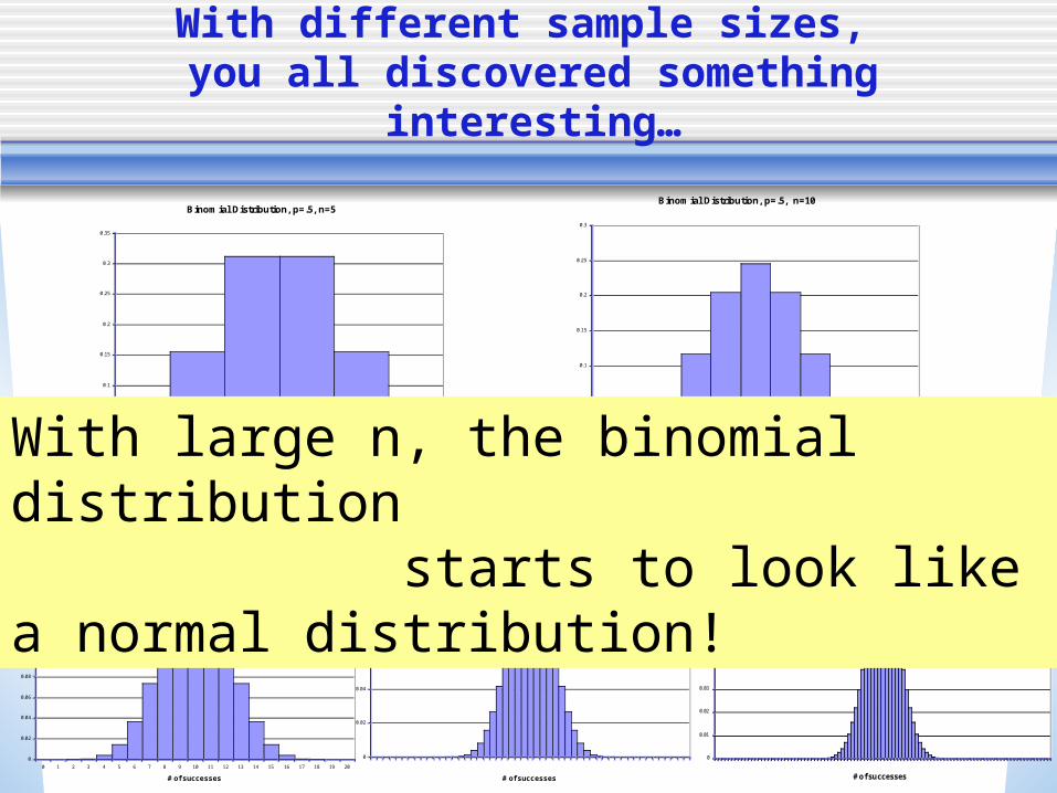
With different sample sizes, you all discovered something interesting…
Binomial Distribution, p=.5, n=10
0
0.05
0.1
0.15
0.2
0.25
0.3
0 1 2 3 4 5 6 7 8 9 10
# of successes
probability
Binomial Distribution, p=.5, n=5
0
0.05
0.1
0.15
0.2
0.25
0.3
0.35
0 1 2 3 4 5
# of successes
probability
Binomial Distribution, p=.5, n=50
0
0.02
0.04
0.06
0.08
0.1
0.12
0 2 4 6 8 10 12 14 16 18 20 22 24 26 28 30 32 34 36 38 40 42 44 46 48 50
# of successes
probability
Binomial Distribution, p=.5, n=100
0
0.01
0.02
0.03
0.04
0.05
0.06
0.07
0.08
0.09
0 3 6 912 15 18 21 24 27 30 33 36 39 42 45 48 51 54 57 60 63 66 69 72 75 78 81 84 87 90 93 96 99
# of successes
probability
Binomial Distribution, p=.5, n=20
0
0.02
0.04
0.06
0.08
0.1
0.12
0.14
0.16
0.18
0.2
0 1 2 3 4 5 6 7 8 9 10 11 12 13 14 15 16 17 18 19 20
# of successes
probability
With large n, the binomial distribution starts to look like a normal distribution!

What is a Normal Distribution?
• Class of distributions with the same overall shape• Continuous probability distribution• defined by two parameters:
mean: stdev: Special:Standard Normal Distribution
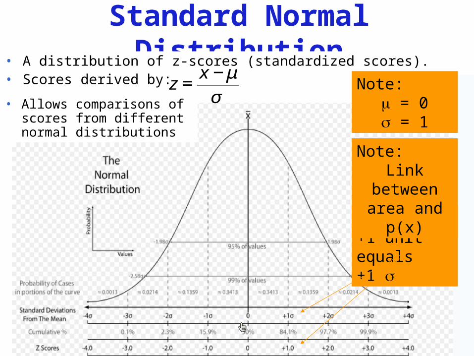
Standard Normal Distribution
Note also:+1 unit equals +1
• A distribution of z-scores (standardized scores).• Scores derived by:
€
z =x − μ
σ• Allows comparisons of scores from different normal distributions
Note: = 0 = 1
Note:Link between area and p(x)
Probability & Standardizing Scores
• The standard normal distribution allows us to easily calculate probabilities for any normal distribution:
• Example: Say that we know that the average checking account balance for a UIUC student is normally distributed with an average balance of $150 and a standard deviation of $125.
• What is the probability of a randomly selected student having a balance of…
• more than $250?• Less than $0• Between $100 and $200?

Why do we care so much about Normal Distributions?
• What happened to the binomial distribution as n increased?
Central Limit TheoremAs the sample size n increases, the distribution of the sample average approaches the normal distribution with a mean µ and variance 2/n irrespective of the shape of the original distribution.

Wait. What?
• Example: Rolling one die, multiple dice… • http://www.stat.sc.edu/~west/javahtml/CLT.html
• So, just like flipping the coin, multiple samples of the sum of the n observations, approaches the normal.
• Since the mean of a sample is the sum of all observations over n (where n is constant for all samples), this same principle applies to the sample mean.

Hmm. Ok…
• But, does the underlying distribution really not matter? http://intuitor.com/statistics/CentralLim.html
• Note that the size of n slightly changed the shape of the normal distribution.
• Also, note that the central limit theorem stated the mean was µ and variance 2/n (so stdev = /√n )
• The variance is a little different than before isn’t it?

T distributions
• To adjust for the fact that the normal distribution is a better approximation for a sampling distribution as n increases, we have the T distribution…
So, the t distribution varies depending on the number of degrees of freedom (n-1)
With lower n, the t distribution is more spread out. This means that getting more extreme values is more probable with low n.

So what good does that do us, anyway?
• Because we can assume that a sampling distribution will be approximately normal with a large n, we can use this distribution to estimate the probability of obtaining a given sample.

Example:(aka excuse to show pictures of my dog)
Notice that we don’t know what the underlying distribution of adoptability scores looks like at this shelter, but because of CLT we can still come upwith an answer.
A large dog shelter in Chicago wants to increase awareness of the adorable pups they have for adoption by bringing some dogs to a local festival. They have 50 people who have volunteered to walk the dogs around the festival. In the shelter there are several hundred dogs. The shelter knows that on average their dogs have a 14 point adoptability score (combination of things like behavior, training, breeding, cuteness, etc.), and the scores tend to vary by about 3. The shelter would prefer to show dogs that have an average of at least a 16 adoptability score. Should they go through all the dogs and select 50 by hand, or are they likely to get a group with this average by chance?

Example:(aka excuse to show pictures of my dog)
A large dog shelter in Chicago wants to increase awareness of the adorable pups they have for adoption by bringing some dogs to a local festival. They have 50 people who have volunteered to walk the dogs around the festival. In the shelter there are several hundred dogs. The shelter knows that on average their dogs have a 14 point adoptability score (combination of things like behavior, training, breeding, cuteness, etc.), and the scores tend to vary by about 3. The shelter would prefer to show dogs that have an average of at least a 16 adoptability score. Should they go through all the dogs and select 50 by hand, or are they likely to get a group with this average by chance?
What information is important here?
µ = 14 = 3X = 16
N = 50

A couple more distributions
• There are 2 more distributions that we will need later.
• ALEKS is familiarizing them with you now so that you know how to use the calculators etc. when it comes up.
• Generally, you should know: Shape of the distribution How to use the distribution practically (at this
point this means using the ALEKS calculator to find the probability of a given value in a distribution)-- so don’t worry
Vague concept of what the distribution means
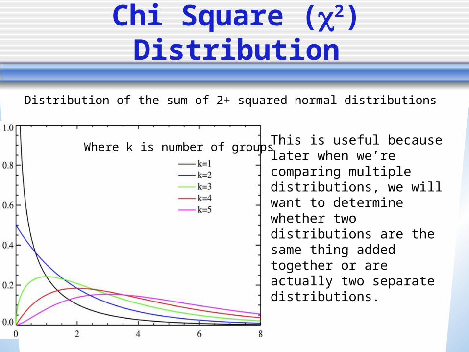
Chi Square (2) Distribution
Distribution of the sum of 2+ squared normal distributions
This is useful because later when we’re comparing multiple distributions, we will want to determine whether two distributions are the same thing added together or are actually two separate distributions.
Where k is number of groups

F distribution
Distribution of the variance of one sample from a normally distributed population divided by the variance of another.
d1 is degrees of freedom of the top (numerator) distributiond2 is degrees of freedom for the bottom (denominator) distribution
This will be useful later when we want to test if there is more variance within a group than across groups (ANOVA)… if there is greater within group variance, then its unlikely that the groupings are meaningful.

Next Week
• Keep up with the content goals• Watch for an email about course
evaluations/suggestions• Please let us know if you want or
need help• If you’ve fallen behind, expect to be
contacted by email.• Have a good week everyone!


