pT rr d pT rr - images.nature.com · (S16) Nature Neuroscience: doi:10.1038/nn.2814. 6 As we did...

1

Near-optimal visual search: behavior and neural basis Wei Ji Ma, Vidhya Navalpakkam, Jeffrey Beck, Ronald van den Berg, Alexandre Pouget Supplementary Results and Figures 1 Theory .......................................................................................................................... 1

1.1 Global log likelihood ratio ................................................................................... 1

1.2 Local log likelihood ratio (neural form) ............................................................... 3

1.3 Local log likelihood ratio (behavioral form) ........................................................ 5

1.4 Relation of optimal model to max and sum models ............................................. 7

1.5 Non-optimal local decision variables ................................................................... 8

2 Behavioral experiments ............................................................................................... 8

2.1 Experiments 1a and 2a ......................................................................................... 8

2.2 Individual-subject ROCs ...................................................................................... 9

2.3 Bayesian model comparison ................................................................................. 9

3 Neural implementation .............................................................................................. 10

3.1 Intuition behind a nonlinearity ........................................................................... 10

3.2 Network performance ......................................................................................... 10

3.3 Effect of non-Poisson-like statistics ................................................................... 11

Supplementary Figures are at the end.

1 Theory

1.1 Global log likelihood ratio Optimal decisions are based on the probabilities of the alternatives given the noisy evidence1. In our experiments, the alternatives are “target absent” (T=0) and “target present” (T=1). We call the variable T global target presence. In this section, we use a formulation of the model in which observations are patterns of neural activity at all N locations, r1,…,rN (Fig. 7a). This formulation is identical to the one discussed in the main text, except that population activity ri is used instead of the scalar internal representation xi. We will relate the scalar representation to population activity in Section 1.3, but the formulation with population activity is more complete because it allows for the automatic encoding of sensory uncertainty. The log likelihood ratio of global target presence (also called global decision variable) is defined as

1

1

, , | 1log

, , | 0N

N

p Td

p T

r r

r r

. (S1)

Nature Neuroscience: doi:10.1038/nn.2814

2

We now review the derivation of the expression for d in terms of locally defined quantities2-4. We assume that given target presence (0 or 1) at each location, the variability in population activity ri is conditionally independent between locations. As a consequence, when the target is absent, the probability of observing r1,…,rN is equal to the product of the probabilities of each pattern ri given that the ith location contains a distractor (Ti=0):

11

, , | 0 | 0 .N

N i ii

p T p T

r r r (S2)

If the target is present, it can be located at any of the N locations. We denote by p(Ti=1|T=1) the probability that location i contains the target in a target-present display. The probability of observing r1,…,rN if the target is present is obtained by marginalizing out target location, i.e., taking a weighted average over all possible target locations:

1 11

, , | 1 1| 1 , , | 1N

N i N ii

p T p T T p T

r r r r . (S3)

The conditional probability p(r1,…,rN|Ti=1) is computed by using the fact that if the target is present at the ith location, then it is absent at all other locations:

11

11

11

, , | 1 1| 1 | 1 | 0

| 1| 0 1| 1

| 0

| 0 1| 1 .i

N

N i i i j ji j i

N Ni i

j j iij i i

N Nd

j j iij

p T p T T p T p T

p Tp T p T T

p T

p T p T T e

r r r r

rr

r

r

(S4)

Here, di is the local log likelihood ratio (also called local decision variable) at location i, defined as

| 1log

| 0i i

ii i

p Td

p T

r

r. (S5)

Dividing Eq. (S4) by Eq. (S2) and taking the log, we find the global log likelihood ratio as

1

log 1| 1 i

Nd

ii

d p T T e

. (S6)


3

Finally, we assume that all locations are equally likely to contain the target and the

observer uses this knowledge, so that p(Ti=1|T=1)=1N. Then Eq. (S6) becomes

1

1log i

Nd

i

d eN

, (S8)

which is Eq. (2) in the main text. If d is positive, the observer’s response is “target present”, otherwise “target absent”; this is maximum-a-posteriori readout. It is important to note that Eq. (S8) holds regardless of the noise model at a given location, p(ri|Ti). It does not depend either on whether we use ri, xi, or some other variable to describe the local observations. The only assumptions we have made are that each location is equally likely to contain the target and that variability is conditionally independent between locations. The next step is to further evaluate the local log likelihood, di.

1.2 Local log likelihood ratio (neural form) Eq. (S5) expresses the local log likelihood ratio in terms of the probabilities of the activity in the ith population, ri, given target absence or presence at that location. These probabilities are obtained by marginalizing over si, the stimulus at that location:

| | 1log

| | 0

i i i i i

i

i i i i i

p s p s T dsd

p s p s T ds

r

r. (S9)

Since the target always has value sT, the numerator is equal to p(ri|sT). When the reliability of the stimulus is unknown, the stimulus likelihood, L(si)=p(ri|si), must be obtained by marginalization over the nuisance parameters ci, such as contrast. The most important feature of Poisson-like variability (Eq. (5) in the main text) is that this marginalization does not affect the form of the stimulus-dependence of the likelihood:

| | ,

,

, .

i i i

i i i

i i i i i i i

si i i i

si i i i

p s p s p d

e p d

p d e

h r

h r

r r c c c

r c c c

r c c c

(S10)

For the local log likelihood ratio, Eq. (S9), this implies


4

, | 1log

, | 0

| 1log .

| 0

i i i

i i i

i i i

i i i

si i i i i i i

i si i i i i i i

si i i

si i i

p d e p s T dsd

p d e p s T ds

e p s T ds

e p s T ds

h r

h r

h r

h r

r c c c

r c c c (S11)

Population activity ri only appears in a specific combination, namely through the local (unnormalized) stimulus likelihood function

| i i isi i iL s p s e h rr .

The width of this stimulus likelihood function is a measure of sensory uncertainty associated with the observation at the ith location on the given trial. The local decision variable, Eq. (S11), and therefore also the global decision variable, are functionals of the stimulus likelihood function5.

Since the target always has value sT, the numerator in the second line of Eq. (S11)

is equal to exp(hi(sT)ri). The denominator depends on the distractor distribution, p(si|Ti=0). We consider the two cases used in our experiments: homogeneous distractors, and heterogeneous distractors drawn from a uniform distribution. Homogeneous distractors In Experiments 1, 1a, and 3, distractors are homogeneous, that is, they all have the same orientation. Moreover, this orientation has the same value, sD, on all trials. (The optimal decision rule is different when the common distractor orientation varies from trial to trial, even if the target-distractor difference is kept constant by varying the target orientation as well.) In other words, the distractor distribution is a delta function. Then we have p(ri|Ti=0)=p(ri|sD), and from Eq. (S5),

|log

|i T

ii D

p sd

p s

r

r. (S12)

When we substitute Poisson-like neural variability with stimulus-dependent kernel hi(s), the local log likelihood ratio becomes

i i T i D id s s h h r . (S13)

In other words, the local log likelihood ratio is a linear combination of the activities of the neurons in the population (Fig. S11a). Although the variance σi

2 does not appear


5

explicitly in Eq. (S13) as it did in Eq. (3) in the main text, it does influence the decision variable. This is because in a probabilistic population code, the gain of ri is inversely

related to the variance, σi2 6. Specifically, the relationship between hi(s)ri, xi, and σi

2 is5

2

2

2

2i i

ii i

s x ss

r

h rr

.

Heterogeneous distractors In Experiments 2 and 4, distractors are heterogeneous and drawn independently from a uniform distribution over orientation, that is, p(si|Ti=0)=1/π. Substituting in Eq. (S11) and assuming Poisson-like variability, we find

0

0

1log log .

1

i T i

i i i

i i i

ss

i i T i is

i

ed s e ds

e ds

h rh r

h rh r (S14)

Unlike the local log likelihood ratio in the homogeneous case, this is a nonlinear function of ri. The integral can, in general, not be evaluated analytically.

1.3 Local log likelihood ratio (behavioral form) We modeled the psychophysics results using the optimal model described above, with the modification that we reduced neural population activity ri to a scalar observation, xi. This scalar observation is the maximum-likelihood estimate of s obtained from the population

activity, ˆi ML ix s r . (This population interpretation is to be contrasted with a previous

interpretation in terms of single-neuron activity7.) The maximum-likelihood estimate can be thought of as a noisy internal representation of the stimulus, that is, xi=si+noise. Using xi instead of ri is simpler, and sufficient to model behavioral experiments, as long as we keep in mind that the uncertainty associated with this observation, σi, is also encoded in ri. The scalar observation xi is assumed to obey a normal distribution centered at the true stimulus orientation, si, with standard deviation σi:

2

22

2

1|

2

i i

i

x s

i i

i

p x s e

. (S15)

We can now express the local log likelihood ratio in terms of xi and σi:

| , | 1| 1,log log

| 0, | , | 0

i i i i i ii i ii

i i i i i i i i i

p x s p s T dsp x Td

p x T p x s p s T ds

. (S16)


6

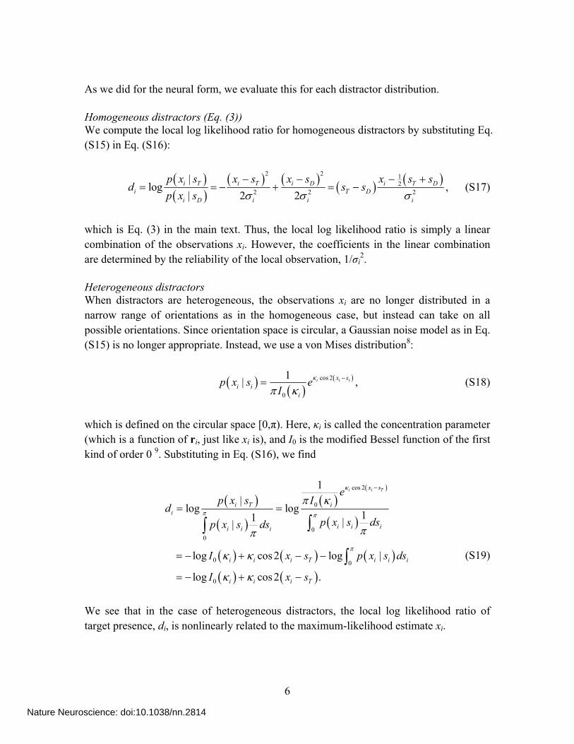
As we did for the neural form, we evaluate this for each distractor distribution. Homogeneous distractors (Eq. (3)) We compute the local log likelihood ratio for homogeneous distractors by substituting Eq. (S15) in Eq. (S16):

2 2 12

2 2 2

|log

| 2 2i T i T i D i T D

i T Di D i i i

p x s x s x s x s sd s s

p x s

, (S17)

which is Eq. (3) in the main text. Thus, the local log likelihood ratio is simply a linear combination of the observations xi. However, the coefficients in the linear combination are determined by the reliability of the local observation, 1/σi

2. Heterogeneous distractors When distractors are heterogeneous, the observations xi are no longer distributed in a narrow range of orientations as in the homogeneous case, but instead can take on all possible orientations. Since orientation space is circular, a Gaussian noise model as in Eq. (S15) is no longer appropriate. Instead, we use a von Mises distribution8:

cos 2

0

1| i i ix s

i ii

p x s eI

, (S18)

which is defined on the circular space [0,π). Here, κi is called the concentration parameter (which is a function of ri, just like xi is), and I0 is the modified Bessel function of the first kind of order 0 9. Substituting in Eq. (S16), we find

cos 2

0

00

0 0

0

1

|log log

11 ||

log cos 2 log |

log cos 2 .

i i Tx s

i T ii

i i ii i i

i i i T i i i

i i i T

ep x s I

dp x s dsp x s ds

I x s p x s ds

I x s

(S19)

We see that in the case of heterogeneous distractors, the local log likelihood ratio of target presence, di, is nonlinearly related to the maximum-likelihood estimate xi.


7

1.4 Relation of optimal model to max and sum models Previous studies of visual search have modeled the rule by which local information gets combined into a global decision variable. They typically assumed fixed target and distractor stimuli, and found that max and sum models often describe human behavior well2, 7, 10-12. Here, we point out their relationships to the optimal model.

In the maxx model, the global decision variable is obtained from local observations through a maximum operation:

max ii

d x . (S20)

In the sumx model, the decision variable is obtained by summing:

1

N

ii

d x

. (S21)

Both simple rules are special cases of the optimal model. Starting from Eq. (S8) for the global log likelihood ratio, we first consider the approximation in which the local log likelihood ratio at one location is substantially larger than at all other locations. Then the sum is dominated by its largest term, and Eq. (S8) becomes

max logii

d d N . (S22)

This is, up to a set size-dependent shift, the maxd decision variable. We saw in Eq. (S17) that if distractors are homogeneous and reliabilities are equal, di is linearly related to xi. In that case, Eq. (S22) is equivalent to the maxx rule, Eq. (S20), except that the optimal decision criterion is now no longer 0.

We next consider the special case in which all di are small in absolute value, |di|<1, which tends to occur when target and distractors are similar. Then we can perform a Taylor series expansion in Eq. (S8), to find

1 1

1 1

1 1log 1 log

1 1log 1 .

N N

i ii i

N N

i ii i

d d N dN N

d dN N

(S24)

This is proportional to the sum of the local log likelihood ratios, and therefore this approximation reduces to the sumd model. Again in the case of homogeneous distractors and equal reliabilities, di is linearly related to xi, and d in Eq. (S24) becomes equivalent to


8

the decision variable of the sumx model, Eq. (S21). It should be noted that the condition |di|<1 is hard to satisfy due to the tails of the Gaussian distribution obeyed by xi. Although the maxx and sumx rules are special cases of the optimal rule, the optimal rule is valid in much greater generality, namely for arbitrary reliabilities and target and distractor distributions.

1.5 Non-optimal local decision variables Here, we specify the maxx, sumx, L

2, and L4 models for heterogeneous distractors. When distractors are homogeneous, the local decision variable in these models is the internal

representation xi, which is drawn from a normal distribution with mean si and variance i2.

For homogeneous distractors, this is a reasonable choice, because coordinates can always be chosen such that the target orientation has a higher value than the distractor orientation, so that a target will tend to produce higher values of xi than a distractor. When distractors are heterogeneous however, the choice of local decision variable in models that do not use the local log likelihood ratio is less simple, since distractors can have all possible orientations. This means that there is no natural coordinate frame in which the target is larger than the distractors. This can be addressed by taking the local decision variable to be the response of a “detector” that responds most strongly to the target7, 13. This idea can be implemented in several ways. We chose a neurally inspired way in which the detector is a Poisson neuron with a Von Mises tuning curve over orientation. Its spike count ri in response to a stimulus si is drawn from a Poisson distribution with mean f(si,gi), where gi is the gain at the ith location (determined by the parameter that manipulates reliability, such as contrast). The mean is given by tuning curve of the neuron:

tc, exp cos 2 1i i i i Tf s g g s s b .

Here, κtc is the concentration parameter of the tuning curve, which we set to 1.5, and b is the baseline activity, which we set to 5.

2 Behavioral experiments

2.1 Experiments 1a and 2a Data were analyzed as in Experiments 1 to 4. ROCs of individual subjects in Experiment 1a are shown in Figure S5, and of Experiment 2a in Figure S6. Solid lines are model fits. MIXED ROC areas and model log likelihoods relative to the optimal model are shown in Figure S9. All values are negative for all subjects, indicating that the optimal model fits best. This is consistent with the results from Experiments 1 to 4.


9

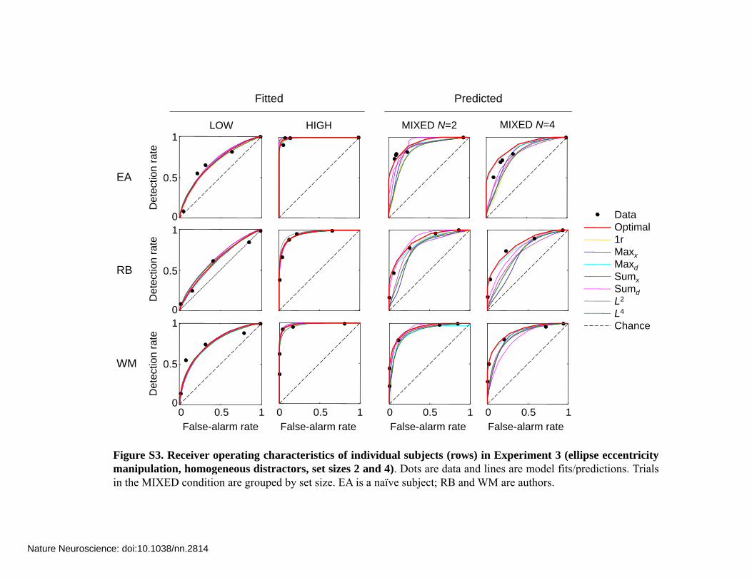
2.2 Individual-subject ROCs Figures S1 to S6 show the predicted ROCs in the MIXED condition for each experiment, each individual subject, and each model. A few remarks:

For a pair of MIXED ROCs conditioned on target reliability (low or high), the same set of “target absent” data was used to obtain the false-alarm rates.

The single-reliability (1r) model produces the same fits in LOW and HIGH as the optimal model. This is expected, since the models are equivalent when reliability is equal across all items and trials.

Partially or wholly below-chance ROCs are due to conditioning on target reliability. Unconditioned ROCs do not go below chance.

Non-concave ROCs for some models arise from a large difference between the fitted reliability values in LOW and HIGH. Unconditioned ROCs for the optimal model are always concave.

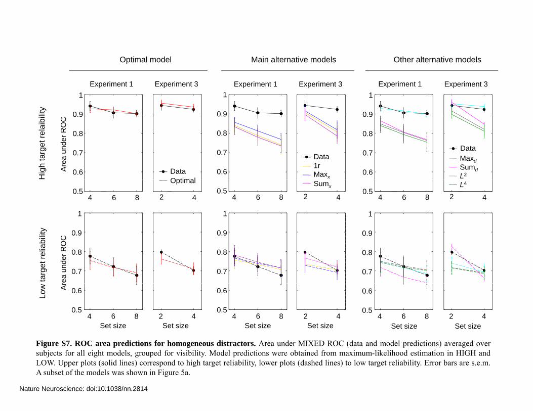
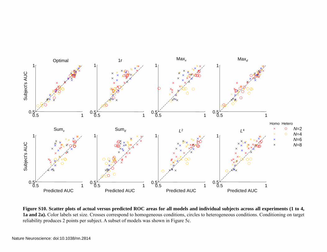
Figure S7 to S9a shows the area under the MIXED ROC (AUC) averaged over subjects, for each experiment, each target reliability condition, and each model. Figure S10 shows for each model, each homogeneity condition (homogeneous or heterogeneous) and each set size a scatter plot of actual versus predicted MIXED ROC area across all individual subjects, all experiments and both target reliability conditions.

We performed a 4-way ANOVA with factors observer type (data or model), stimulus type (bar or ellipse), distractor type (homogeneous or heterogeneous), and target reliability (low or high) on the combined AUC data of all six experiments. Main effects of observer type are shown in Table S1. No main effect or interactions were found for the optimal and maxd model.

Table S1: Main effect of observer type on AUC across all experiments, for each model

Model Main effect of observer type Conclusion

optimal F(1,108) = 0.14, p = 0.71 - 1r F(1,108) = 10.18, p = 0.0019 ruled out maxx F(1,108) = 21.64, p < 0.0001 ruled out maxd F(1,108) = 0.05, p = 0.82 - sumx F(1,108) = 29.16, p < 0.0001 ruled out sumd F(1,108) = 16.81, p < 0.0001 ruled out L2 F(1,108) = 24.63, p < 0.0001 ruled out L4 F(1,108) = 26.16, p < 0.0001 ruled out

2.3 Bayesian model comparison Table S2 shows the results of Bayesian model comparison. Values are means s.e.m. across subjects. The factor by which the optimal model is more likely than the alternative


10

model is given by the exponential of a value in the table. The optimal model is most likely across all experiments and all alternative models. Table S2: Log likelihood of the optimal model minus the likelihood of each alternative model (columns) for each experiment (row). Mean and standard error across subjects. 1r maxx maxd sumx sumd L2 L4 1 28.0 ± 1.8 14.4 ± 3.0 25.9 ± 2.2 30.9 ± 2.2 29.1 ± 1.5 22.6 ± 1.6 22.6 ± 2.32 11.4 ± 1.6 10.1 ± 3.9 8.6 ± 0.8 25.1 ± 5.4 6.1 ± 1.6 16.6 ± 5.0 12.3 ± 4.43 14.5 ± 3.1 14.1 ± 4.0 5.6 ± 0.6 18.9 ± 5.1 10.2 ± 1.7 21 ± 11 19.9 ± 9.84 14.0 ± 4.0 24.2 ± 3.5 56 ± 20 22.1 ± 4.7 16.3 ± 3.8 22.3 ± 5.0 25.1 ± 4.21a 7.5 ± 1.2 8.1 ± 0.9 5.2 ± 0.8 8.8 ± 0.1 4.8 ± 1.1 8.7 ± 1.6 8.6 ± 1.92a 11.1 ± 4.6 21.0 ± 7.0 60 ± 11 23.6 ± 2.6 31.2 ± 5.4 22.7 ± 4.6 24.2 ± 4.4

3 Neural implementation

3.1 Intuition behind a nonlinearity Figure S11c illustrates why marginalizing over distractor orientation requires a nonlinear operation when distractors are heterogeneous. We simulated a large number of population patterns of activity at a single location, with gain randomly drawn from a large range and orientation drawn from a uniform distribution. For every pattern, we took the inner product with the vector formed by the cosines of twice the preferred orientations of the neurons in the population, and with the vector formed by their sines (the factor 2 serves

to map orientation space [0,) onto the circle). The resulting vector is commonly known

at the population vector14. The target, assumed to be at 0, is detected if the second layer responds strongly whenever the point falls within the cone-shaped region delimited by the red parabola. This can be achieved if the second layer uses a quadratic nonlinearity, since a parabola is a quadratic function. When distractors are homogeneous, a linear boundary in activity space suffices.

3.2 Network performance Scatter plots shown in Figures 7c-d, S12-14 demonstrate the manner in which the tested networks fail to accurately represent the optimal posterior distribution. Bias is indicated by a deviation from the diagonal and lack of reliability by a large variance. In all cases, the network parameters were learned as described above.

Figure S12 shows network results for the first marginalization when distractors are homogeneous. As indicated in the main text, a Poisson-like probabilistic population code already exists in the input layer in this case. Since all tested networks include a purely linear network as a subset, it is not surprising that for all of the tested networks, learning converged to the optimal solution.

Figure S13 shows network results for the first marginalization when distractors are heterogeneous. In this case, the optimal decision boundary is nearly quadratic (Fig. 7b) and the linear networks (LIN and LDN) fail. The quadratic network (QUAD) is capable


11

of consistently representing the true probability only when contrast is known. This is indicated by a reliable, monotonic relationship between the network-estimated probability and the true probability of target presence when conditioned on contrast (Fig. 7c left panel, or Fig. S13b). Indeed, if we present only a single value of contrast when learning the network parameters, the approximation to the posterior estimated by the quadratic network is unbiased (not shown). While a quadratic nonlinearity allows the second layer to discriminate between a target and a distractor, it fails to satisfy the requirement that all layers use Poisson-like probabilistic population codes. The right panel of Figure 7c (S13d) shows that the addition of divisive normalization to the quadratic network (QDN) is sufficient to eliminate the need to know the contrast of the stimulus in order to reliably estimate the posterior over target presence. Intuitively, one could say that the function of the divisive normalization is to properly scale the network output so that the distance from the decision bound in Figure 7b is proportional to the log likelihood ratio.

The same trends hold for the marginalization over target location between the second and third layer, as shown in Figures 7d and S14. Specifically, note that the LIN and LDN networks are both biased (systematic deviation from the diagonal) and unreliable (large variance). The QUAD network is quite reliable but biased. It is unbiased when the local contrasts are known (not shown). Using a quadratic nonlinearity with divisive normalization (QDN), the third layer encodes a low-variance and unbiased estimate of the optimal posterior. Figure S15 indicates that the QDN network loses less information than the other tested networks on both marginalizations.

3.3 Effect of non-Poisson-like statistics The Poisson-like statistics of the input population represent a sufficient condition for the optimality of the QDN networks used to implement inference in this task. In order to give some insight into the reason for our choice of Poisson-like statistics, it is useful to consider a situation in which optimal inference fails due to non-Poisson-like statistics of the inputs. Recall that a Poisson-like population code representation of a posterior distribution results from a likelihood which can be parameterized by

| , , exp ( )p s c c s r r h r , (S25)

where the stimulus-dependent kernel, h(s), depends only on s and not on nuisance parameters such as contrast, denoted by c. This restriction on h(s) is non-trivial as h(s) is related to two quantities which often do depend on the nuisance parameter c, namely the tuning curve, f(s,c), and covariance, Σ(s,c), according to the equation

1'( ) ( , ) '( , )s s c s ch Σ f , (S26)

where the prime denotes a derivative with respect to the stimulus s.


12

We repeated the procedure used to demonstrate the near-optimality of the QDN network (and the suboptimality of the other networks) on an input population which does not satisfy this characteristic of a Poisson-like population. In particular, we continued to use input neurons whose activity is independent and Poisson, but now assumed that an increase in contrast modulates the width of the tuning curve, rather than its amplitude. Thus, the gain parameter g was fixed and the concentration parameter κtc was contrast-dependent:

tc, exp cos 2 1j jf s c g c s s . (S27)

For populations of independent Poisson neurons, the stimulus-dependent kernel is given

by the log of the tuning curve, i.e., tc, log cos 2 1j jh s c g c s s . Its

derivative with respect to s depends on c, and therefore the input population is not Poisson-like.

We showed that when the input population was Poisson-like and distractors were homogeneous, all networks were capable of near-optimal marginalization over orientation (Fig. S15a). This was because the input population was already a Poisson-like code for target presence. This is not the case when the stimulus-dependent kernel depends on contrast and the variability therefore deviates from Poisson-like. For instance, the linear network (LIN) is no longer capable of performing optimal inference (Fig. S16a, LIN). The QDN network, however, is capable of performing near-optimal inference (Fig. S16a, QDN) because it implements a marginalization over contrast rather than over distractor distribution (since the marginalization over distractors is trivial in this case). By contrast, all networks, including QDN, are suboptimal when the distractor distribution is uniform (Fig. S16b). This is because we are effectively asking the networks to implement two marginalizations, one over contrast and one over the distractor distribution, which it cannot do:

| | , |i i i i i i i i i ip T p s c p s T p c ds dc r r .

Compare this to Eq. (S11), where the contrast dependence factorizes out. A comparison of Figures S15a and S16c reinforces this point: while the QDN network lost less than 2% information in the heteregenous case with Poisson-like variability, the information loss jumped close to 30% when the variability was no longer Poisson-like. 1. Green, D.M. & Swets, J.A. Signal detection theory and psychophysics (John Wiley & Sons, Los Altos, CA, 1966). 2. Palmer, J., Verghese, P. & Pavel, M. The psychophysics of visual search. Vision Res 40, 1227-1268 (2000). 3. Peterson, W.W., Birdsall, T.G. & Fox, W.C. The theory of signal detectability. Transactions IRE Profession Group on Information Theory, PGIT-4, 171-212 (1954).


13

4. Nolte, L.W. & Jaarsma, D. More on the detection of one of M orthogonal signals. J Acoust Soc Am 41, 497-505 (1966). 5. Ma, W.J. Signal detection theory, uncertainty, and Poisson-like population codes. Vision Res 50, 2308-2319 (2010). 6. Ma, W.J., Beck, J.M., Latham, P.E. & Pouget, A. Bayesian inference with probabilistic population codes. Nat Neurosci 9, 1432-1438 (2006). 7. Verghese, P. Visual search and attention: a signal detection theory approach. Neuron 31, 523-535 (2001). 8. Mardia, K.V. & Jupp, P.E. Directional statistics (Wiley, 1999). 9. Abramowitz, M. & Stegun, I.A. eds. Handbook of mathematical functions (Dover Publications, New York, 1972). 10. Eckstein, M.P., Thomas, J.P., Palmer, J. & Shimozaki, S.S. A signal detection model predicts the effects of set size on visual search accuracy for feature, conjunction, triple conjunction, and disjunction displays. Percept Psychophys 62, 425-451 (2000). 11. Baldassi, S. & Verghese, P. Comparing integration rules in visual search. J Vision 2, 559-570 (2002). 12. Graham, N., Kramer, P. & Yager, D. Signal dection models for multidimensional stimuli: probability distributions and combination rules. J Math Psych 31, 366-409 (1987). 13. Eckstein, M.P., Peterson, M.F., Pham, B.T. & Droll, J.A. Statistical decision theory to relate neurons to behavior in the study of covert visual attention. Vision Res 49, 1097-1128 (2009). 14. Georgopoulos, A., Kalaska, J., Caminiti, R. & Massey, J.T. On the relations between the direction of two-dimensional arm movements and cell discharge in primate motor cortex. J. Neurosci. 2, 1527-1537 (1982).


LOW HIGH MIXED N=4 MIXED N=6 MIXED N=81

rate

Fitted Predicted

DB

1

0

0.5D

etec

tion

r

JB

0

1

0.5

Det

ectio

n ra

te

Optimal1rMax

Data

SN

1

0.5

0

tect

ion

rate

MaxxMaxdSumxSumdL2

L4

Chance

VN

10

Det

on r

ate

Chance

VN

0

0.5

0 10.5 0 10.5 0 10.5 0 10.5 0 10.5

Det

ectio

False-alarm rate False-alarm rate False-alarm rate False-alarm rate False-alarm rate

Figure S1. Receiver operating characteristics of individual subjects (rows) in Experiment 1 (bar contrast manipulation,homogeneous distractors, set sizes 4, 6, and 8). Dots are data and lines are model fits/predictions. Trials in the MIXED condition aregrouped by set size. DB and SN are naïve subjects; JB and VN are authors. Subject SN is also shown in Figures 4a and 8a.


LOW HIGHMIXED

Target low reliability1

te

MIXEDTarget high reliability

MIXEDAll

Fitted Predicted

AI

0

0.5

Det

ectio

n ra

t

MD

1

0.5

etec

tion

rate

Optimal1rMax

Data

VB

1

0.5

0

Dct

ion

rate

MaxxMaxdSumxSumdL2

L4

Chance

10

Det

ecra

te

Chance

VN

0

0.5

0 10.5 0 10.5 0 10.5 0 10.5 0 10.5

Det

ectio

n


Figure S2. Receiver operating characteristics of individual subjects (rows) in Experiment 2 (bar contrast manipulation, heterogeneousdistractors, set size 4). Dots are data and lines are model fits/predictions. Fewer than five dots in a plot means that the subject did not use allpossible responses (present/absent × confidence ratings). Trials in the MIXED condition are grouped by target reliability. AI, MD, and VB arenaïve subjects; VN is an author (also shown in Figures 4b and 8b). Below-chance ROCs are due to conditioning on target reliability.


Fitted Predicted

LOW HIGH MIXED N=2 MIXED N=4

EA

1

0.5tion

rate

EA

10

0.5

Det

ect

rate

Optimal1rMax

Data

RB

10

0.5

Det

ectio

n r Maxx

MaxdSumxSumdL2

L4

Chance

WM

0

0.5

Det

ectio

n ra

te

Chance

00 10.5 0 10.5 0 10.5 0 10.5False-alarm rate False-alarm rate False-alarm rate False-alarm rate

Figure S3. Receiver operating characteristics of individual subjects (rows) in Experiment 3 (ellipse eccentricitymanipulation, homogeneous distractors, set sizes 2 and 4). Dots are data and lines are model fits/predictions. Trialsp , g , ) pin the MIXED condition are grouped by set size. EA is a naïve subject; RB and WM are authors.


MIXED MIXEDMIXED

Fitted Predicted

LOW HIGH

EA

1

0.5

ectio

n ra

teTarget low reliability Target high reliabilityAll

10

Det

en

rate Optimal

1rMax

Data

RB

10

0.5

Det

ectio

e

MaxxMaxdSumxSumdL2

L4

Chance

WM

0

0.5

0 10 5 0 10 5 0 10 5 0 10 5

Det

ectio

n ra

te

0 10 5

Chance

0 10.5 0 10.5 0 10.5 0 10.5

False-alarm rate False-alarm rate False-alarm rate False-alarm rate

Figure S4. Receiver operating characteristics of individual subjects (rows) in Experiment 4 (ellipse eccentricity manipulation,heterogeneous distractors set size 2) Dots are data and lines are model fits/predictions Trials in the MIXED condition are grouped

False-alarm rate

0 10.5

heterogeneous distractors, set size 2). Dots are data and lines are model fits/predictions. Trials in the MIXED condition are groupedby target reliability. EA is a naïve subject; RB and WM are authors. Below-chance ROCs are due to conditioning on target reliability,non-concave ones are due to a large difference in the fitted parameters glow and ghigh.


LOW HIGHMIXED MIXEDMIXED

Fitted Predicted

LOW HIGH

RB

1

0.5

ectio

n ra

teTarget low reliability Target high reliabilityAll

10

Det

eon

rat

e Optimal1rMax

Data

SK

10

0.5

Det

ectio

te

MaxxMaxdSumxSumdL2

L4

Chance

WM

0

0.5

0 10 5 0 10 5 0 10 5 0 10 5

Det

ectio

n ra

t

0 10 5

Chance

0 10.5 0 10.5 0 10.5 0 10.5


0 10.5

Figure S5. Receiver operating characteristics of individual subjects (rows) in Experiment 1a (bar contrast manipulation,homogeneous distractors, set size 2). Dots are data and lines are model fits/predictions. SK is a naïve subject; RB and WM areauthors.


Fitted Predicted

LOW HIGHMIXED

Target low reliabilityMIXED

Target high reliabilityMIXED

All

RB

1

0 5ion

rate

RB

10

0.5

Det

ect

rate

Optimal1rMax

Data

SK

10

0.5

Det

ectio

n r Maxx

MaxdSumxSumdL2

L4

Chance

WM

1

0.5

Det

ectio

n ra

te

Chance

0 10.5 0 10.5 0 10.5

False-alarm rate False-alarm rate False-alarm rate

Figure S6. Receiver operating characteristics of individual subjects (rows) in Experiment 2a (bar contrast manipulation,

0 10.5 0 10.5

False-alarm rateFalse-alarm rate

0

heterogeneous distractors, set size 2). Dots are data and lines are model fits/predictions. SK is a naïve subject; RB and WM areauthors. Below-chance ROCs are due to conditioning on target reliability, non-concave ones are due to a large difference in the fittedparameters glow and ghigh.


Optimal model Main alternative models Other alternative models

0.9

1

RO

C

Experiment 1 Experiment 3

0.9

1


aibi

lity

0.9

1


0.6

0.7

0.8

Are

a un

der

R

0.6

0.7

0.8

OptimalData

1rMaxx

Data

Hig

h ta

rget

rel

a

0.6

0.7

0.8

MaxdSumdL2

Data

0.54 6 8 2 4

0.54 6 8 2 4

0 9

1

Optimal Sumx

0 9

1

y

0.54 6 8 2 4

L4

0 9

1

0.7

0.8

0.9

0.7

0.8

0.9

rea

unde

r R

OC

targ

et r

elia

bilit

y

0.7

0.8

0.9

0.5

0.6

4 6 8Set size

2 4Set size

0.5

0.6Ar

4 6 8Set size

2 4Set size

Low

0.5

0.6

Set size4 6 8 2 4

Set size

Figure S7. ROC area predictions for homogeneous distractors. Area under MIXED ROC (data and model predictions) averaged oversubjects for all eight models, grouped for visibility. Model predictions were obtained from maximum-likelihood estimation in HIGH andLOW. Upper plots (solid lines) correspond to high target reliability, lower plots (dashed lines) to low target reliability. Error bars are s.e.m.A subset of the models was shown in Figure 5a.


Experiment 2 Experiment 41 1

nder

RO

C optimal1rmaxxmaxd

data

0 6

0.8

1

0 6

0.8

1

nder

RO

C

low high low high

Are

a un d

sumxsumdL2

L40.4

0.6

0.4

0.6

Are

a un

Target reliability Target reliabilitylow high low high

Figure S8. ROC area predictions for heterogeneous distractors. Area under MIXED ROC (data andmodels) averaged over subjects in Experiments 2 and 4. Error bars are s.e.m. A subset of models was shown inFigure 5b.g


a1

data

Experiment 1a Experiment 2a1

b

Are

a un

der

RO

C

0.6

0.8optimal1rmaxxmaxdsumxsumd

Are

a un

der

RO

C

0.6

0.8

c d

A

0.4

Target reliabilitylow high

L2

L4

A

0.4

Target reliabilitylow high

0 0

log

likel

ihoo

d

log

likel

ihoo

d

-20

-40

-10

-80

Rel

ativ

e m

odel

Rel

ativ

e m

odel

-60

-40

1r maxx L2maxd sumx sumd L4

Figure S9. Model comparison at set size 2 (bar stimuli), Experiments 1a and 2a. (a) Area under ROC (dataand models) in Experiment 1a, averaged over subjects. Error bars are s.e.m. (b) Same for Experiment 2a. (c) Loglikelihood of alternative models minus that of the optimal model for individual subjects, obtained through

1r maxx L2maxd sumx sumd L4

Bayesian model comparison, in Experiment 1a (homogeneous distractors). (d) Same for Experiment 2a(heterogeneous distractors).


1

AU

C

Optimal1

1r1

Maxx

1

Maxd

Sub

ject

's A

0.5 10.5

0.5 10.5

0.5 10.5

0.5 10.5

1

Sumx

1

Sumd

1L2

1L4

N=6N=4N=2

Homo Hetero

Sub

ject

's A

UC N=8

0.5 10.5

Predicted AUC0.5 1

0.5

Predicted AUC0.5 1

0.5

Predicted AUC0.5 1

0.5

Predicted AUC

Figure S10. Scatter plots of actual versus predicted ROC areas for all models and individual subjects across all experiments (1 to 4,1a and 2a). Color labels set size. Crosses correspond to homogeneous conditions, circles to heterogeneous conditions. Conditioning on targetreliability produces 2 points per subject. A subset of models was shown in Figure 5c.


b6

aΔh

Orientation0

-1

Ker

nel v

alue

Con

trib

utio

n (%

)

2

4

h(sT) h(sD)

Orientation

0

90

e pr

ojec

tion

-90 -45 0 45 90-2

Preferred orientationC

-90 -45 0 45 90

Preferred orientation

0

Fi S11 P l ti di d i l h ( ) O i t ti d d t k l f t t ( 0° ) d

-90Cosine projection

Sin

e

Figure S11. Population coding and visual search. (a) Orientation-dependent kernels for target (sT=0°; green) anddistractor (sD=10°; yellow) orientations, and their difference Δh (blue). To compute these, we assumed independentPoisson neurons with von Mises tuning curves, fj(s)=g exp(tc cos(s-sj

pref)-1), where g is gain, sjpref is the preferred

orientation of the jth neuron, and κtc=2. The log likelihood ratio of local target presence is the inner product of Δh with asingle-trial population pattern of activity. (b) We quantified the contribution of each preferred orientation by sequentiallyremoving the corresponding neuron from all populations and computing the reduction in percentage correct on theremoving the corresponding neuron from all populations and computing the reduction in percentage correct on thesimulated search task (N=4, g=1.4, 105 trials). Blue: homogeneous distractors (sT=0°, sD=10°), green: heterogeneousdistractors (sT=0°). (c) Motivation for quadratic operations. Scatter plot of population vectors obtained from populationactivity. Dot color indicates presented orientation; gain was drawn randomly from a wide range. In the heterogeneouscondition, the target (green line, here at 0°) must be discriminated from distractors whose orientations are drawn from auniform distribution. The red line indicates a quadratic decision boundary.


1

stim

ate

a b

QUADLIN1

stim

ate

0.5

wor

k po

ster

ior

es

0.5

wor

k po

ster

ior

es

0 0.5 10N

etw

Optimal posteriorc d

LDN QDN

0 0.5 10N

etw

Optimal posterior

1

mat

e 1

mat

e

LDN QDN

0.5

rk p

oste

rior

est

im

0.5

k po

ster

ior

estim

0 0.5 10N

etw

or

Optimal posterior0 0.5 1

0Net

wor

Optimal posterior

Stimulus contrast: Low High

Figure S12. Performance of four networks in approximating optimaltarget detection at one location (homogeneous distractors). Posteriorprobability of local target presence encoded in the second layer of thenetwork versus the optimal posterior. Networks are characterized by their


operation types: LIN – linear; QUAD – quadratic; LDN – linear withdivisive normalization; QDN – quadratic with divisive normalization.Color indicates stimulus contrast.


1

mat

e

a b

QUADLIN1

mat

e

0.5

rk p

oste

rior

estim

Q

0.5

rk p

oste

rior

estim

0 0.5 10N

etw

oOptimal posterior

c d

0 0.5 10N

etw

o

Optimal posterior

1

ate 1

ate

LDN QDN

0.5

post

erio

r es

tima

0.5

post

erio

r es

tima

0 0.5 10N

etw

ork


0Net

wor

k Optimal posterior

Figure S13. Performance of four networks in approximating optimalmarginalization over distractor orientation (heterogeneousdistractors). Posterior probability of local target presence encoded in the


second layer of the network versus the optimal posterior. Networkcharacterizations are as in Figure S12. Color indicates stimulus contrast.Note that panels b and d are identical to the plots shown in Figure 7c.


1

timat

e

a b

QUADLIN1

timat

e

0.5

ork

post

erio

r es

t

0.5

ork

post

erio

r es

t

0 0.5 10N

etw

oOptimal posterior

c d

LDN

0 0.5 10N

etw

o

Optimal posterior

1

ate 1

ate

LDN QDN

0.5

k po

ster

ior

estim

a

0.5

k po

ster

ior

estim

a

0 0.5 10N

etw

ork


0Net

wor

kOptimal posterior

Figure S14. Performance of four networks in approximating optimalmarginalization over target location. Posterior probability of globaltarget presence encoded in the third layer of the network versus the

ti l t i Thi t ti i id ti l f h d

Average contrast: MediumLow High

optimal posterior. This computation is identical for homogeneous andheterogeneous distractors. Color indicates average contrast in the display.Set size was chosen 6. Note that panels b and d are identical to the plotsshown in Figure 7d.


HomogeneousN=4N=6

a b

30m

atio

n lo

ss

HomogeneousHeterogeneous

40

60

mat

ion

loss

N 6N=8

10

20

erce

ntag

e in

form

20

erce

ntag

e in

form

Figure S15. Information loss of four networks. (a) Percentageinformation loss of all networks in the computation of local target

0Pe

0P

LDN QDNQUADLINLDN QDNQUADLIN

information loss of all networks in the computation of local targetpresence, for homogeneous and heterogeneous distractors. (b)Percentage information loss of all networks in the computation of globaltarget presence, for each set size. This computation is identical forhomogeneous and heterogeneous distractors.


stim

ate LIN QUAD LDN QDNa

11 11

wor

k po

ster

ior

e

0.50.5 0.50.5

Net

w

b0 0.5 1 0 0.5 10 0.5 10 0.5 1

r es

timat

e 1

00 00

111

0 0 5 1 0 0 5 10 0 5 10 0 5 1Net

wor

k po

ster

io

0

0.5

0

0.5

0

0.5

0

0.5

Figure S16. Effect of a deviation from Poisson-like variability in the inputon the marginalization over distractor orientation. (a) Posterior probability

0 0.5 1Optimal posterior

c




N

60

HomogeneousHeterogeneous

oss

g ( ) p yof local target presence encoded in the second layer of the network versus theoptimal posterior, when distractors are homogeneous. Color indicates contrast.Each network has been trained. (b) Same for heterogeneous distractors. (c)Percentage information loss of all networks in computing local target presence,for homogeneous and heterogeneous distracters. Comparing to Figure S15a, it20

30

40

50

age

info

rmat

ion

lo

is clear that when the neural variability is no longer Poisson-like, none of thenetworks are near-optimal.

LIN QDN0

10

LDNQUADPer

cent

a


Date post:	05-Nov-2018
Category:	Documents
Upload:	vohuong
View:	218 times
Download:	0 times

pT rr d pT rr - images.nature.com · (S16) Nature Neuroscience: doi:10.1038/nn.2814. 6 As we did...

Documents