Case Study: Model for Economic Lifetime ofDrilling Machines in the Swedish Mining Industry
Hussan Al-Chalabi, Jan Lundberg, Alireza Ahmadi & Adam Jonsson
To cite this article: Hussan Al-Chalabi, Jan Lundberg, Alireza Ahmadi & Adam Jonsson (2015)Case Study: Model for Economic Lifetime of Drilling Machines in the Swedish Mining Industry,The Engineering Economist, 60:2, 138-154, DOI: 10.1080/0013791X.2014.952466
To link to this article: http://dx.doi.org/10.1080/0013791X.2014.952466
The Engineering Economist, 60:138–154, 2015Published with license by Taylor & Francis Group, LLCISSN: 0013-791X print/1547-2701 onlineDOI: 10.1080/0013791X.2014.952466
Case Study: Model for Economic Lifetime of DrillingMachines in the Swedish Mining Industry
HUSSAN AL-CHALABI,1 JAN LUNDBERG,2
ALIREZA AHMADI,2 AND ADAM JONSSON3
1Division of Operation, Maintenance and Acoustics, Lulea Universityof Technology, Lulea, Sweden and Mechanical Engineering Department,College of Engineering, University of Mosul, Mosul, Iraq2Division of Operation, Maintenance and Acoustics, Lulea Universityof Technology, Lulea, Sweden3Division of Mathematic Science, Lulea University of Technology, Lulea,Sweden
The purpose of this article is to develop a practical economic replacement decisionmodel to identify the economic lifetime of a mining drilling machine. A data-drivenoptimization model was developed for operating and maintenance costs, purchase price,and machine resale value. Equivalent present value of these costs by using discount ratewas considered. The proposed model shows that the absolute optimal replacement time(ORT) of a drilling machine used in one underground mine in Sweden is 115 months.Sensitivity and regression analysis show that the maintenance cost has the largest impacton the ORT of this machine. The proposed decision-making model is applicable anduseful and can be implemented within the mining industry.
Introduction
Economic globalization increases competition among mining companies, pushing them toachieve higher production rates by increasing automation and mechanization and using newand more effective equipment. This forces companies to use more reliable capital equipmentwith higher performance capabilities; naturally, these are more expensive. The equipmentused in underground mining industries is subject to degradation throughout its operatinglife. This increases the operating and maintenance costs and reduces production rates,causing a negative economic effect. In addition, the equipment used in underground miningis subject to a harsh working environment, and this accelerates degradation. Given all ofthese factors, key questions for the mining industry include the following. When shouldthe company replace the equipment to minimize cost? How can the maintenance manager
medium, provided the original work is properly attributed, cited, and is not altered, transformed, orbuilt upon in any way, is permitted. The moral rights of the named author(s) have been asserted.
Address correspondence to Hussan Al-Chalabi, Division of Operation, Maintenance and Acous-tics, Lulea University of Technology, Lulea 97187, Sweden. E-mail: [email protected]
138
Dow
nloa
ded
by [
Lul
ea U
nive
rsity
of
Tec
hnol
ogy]
at 0
0:35
05
Nov
embe
r 20
15
Model for Economic Lifetime of Drilling Machines 139
convince finance and production managers to replace capital equipment at a specified timein its life cycle? To answer these questions, life cycle cost analysis should be done inadvance of an equipment replacement decision.
The optimum replacement age of equipment is defined as the time at which the total costis at its minimum value (Jardine and Tsang 2006). In the mining industry, the costs associatedwith owning equipment can be grouped into categories: initial purchase, installation, directdowntime, maintenance and operating, financing, and cost recovery on disposal. The sumof these costs represents the total cost required to own the mining equipment (Hall 2007).Life cycle cost analysis helps decision makers justify equipment replacement on the basisof the total costs over the equipment’s useful life. It allows the maintenance manager tospecify the optimal replacement time at the time of the equipment’s purchase.
Cost function models can be allocated to the various categories to allow easy estimationof the total cost. Such models can be generally classified as detailed models, analogousmodels, and parametric models. A detailed model uses estimates of material quantitiesand prices, labor time, and rates to estimate the direct costs of equipment. Analogousmodels identify similar equipment and adjust costs to account for differences between itand the target equipment. Cost estimation with a parametric model is based on predictingthe equipment’s total cost by using regression analysis based on technical informationand historical cost (Asiedu 1998). Life cycle cost (LCC) analysis should not be seen asa method for defining the total cost of the equipment but as a help in decision making;thus, LCC analysis should be restricted to costs that can be controlled. In general, LCCis determined by summing up all of the potential costs associated with equipment over itslifetime. It is well known that the value of expenditure today costs more than the same valueof expenditure next year because of the “time value of money.” A discount rate is usedto take into consideration the time value of money. To compare costs incurred at differenttimes we must shift expenditure to a reference point in time. Thus, in this article, we areinterested in estimating the equivalent present value of earlier or future costs.
Literature Survey
Standard models for economic replacement time decision contain an estimation of the dis-counted costs by minimizing the LCC of the equipment. The assumption of these modelsis that equipment will be replaced at the end of its economic lifetime by a continuous se-quence of identical equipment (Hartman and Tan 2014). Recently, a number of researchershave studied the economic lifetime of capital equipment. Some consider the optimal life-time of capital equipment using economic theories and vintage capital models, representedmathematically by nonlinear Volterra integral equations with unknown limits of integration(Boucekkine et al. 1997; Cooley et al. 1997; Hritonenko 2005; Hritonenko and Yatsenko2003; Yatsenko 2005). Others use the theory of dynamic programming considering tech-nological changes under finite and infinite horizons (Bellman 1955; Bethuyne 1998; Eltonand Gruber 1976; Hartman 2005; Hritonenko and Yatsenko 2008; Mardin and Arai 2012).Yatsenko and Hritonenko (2005) studied the lifetime optimization of capital equipmentusing integral models. The study designs a general investigation framework for optimalcontrol of the models. Hritonenko and Yatsenko (2007) studied optimal equipment replace-ment without paradoxes. Using an integral model to calculate the economic lifetime ofequipment and considering technological changes (TCs), they showed that the economiclifetime of equipment is shorter when the embodied TC is more intense. Hartman andMurphy (2006) offered a dynamic programming approach to the finite-horizon equipment
Dow
nloa
ded
by [
Lul
ea U
nive
rsity
of
Tec
hnol
ogy]
at 0
0:35
05
Nov
embe
r 20
15
140 H. Al-Chalabi et al.
replacement problem with stationary cost. Their model studies the relationship between theinfinite-horizon solution (continuous replacement of equipment at the end of its economiclifetime) and the finite-horizon solution. Hritonenko and Yatsenko (2009) constructed acomputational algorithm to solve a nonlinear integral equation. The solution is importantfor finding the optimal policy of equipment replacement under technological advances.Karri (2007) considered the optimal replacement time of an old machine, using an opti-mization model that minimizes the machine cost. The model is built to handle capacityexpansion and replacement situations. Using real costs without inflation, Karri (2007) mod-eled the costs of the old machine with simple linear functions. He also used an optimizationmodel that maximizes profit. Scarf and Bouamra (1999) addressed the capital replacementproblem using a discounted cost criterion over a finite time horizon. They presented a robustapproach to solving the fleet replacement problem in which the fleet size is allowed to varyat replacement. A survey of multiple and single asset solution techniques under a variety ofsettings, including tax, variable utilization, various uncertainties, and technological change,was addressed by Hartman and Tan (2014). They also illustrated a number of open problemsthat are worthy of future research. Generally speaking, these studies focus on estimatingthe economic lifetime of equipment, considering technological changes and using integralmodels, theories of dynamic programming, vintage capital models, and algorithms to solvenonlinear integral equations.
Despite the available information, it can be difficult for users to implement complexmodels to calculate the optimal replacement time of equipment. Moreover, these modelssometimes require specific types of data that, as in our case study, are not available. Thesecan include data on production output, technological labor/output coefficient, revenue,profit, etc. Thus, the aim of this study is to identify the replacement age of a mining drillingmachine from an economic point of view, using available data from a mining company,specifically, the operating and maintenance costs, purchase price, and machine resale value.In this study, equivalent present value of these costs was considered by using a discount rate.
Description of Drilling Machine
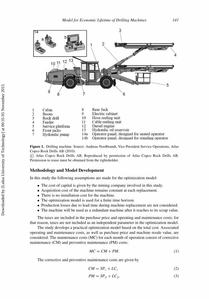
The drilling machines typically used in mines are manufactured by different companiesand have different technical characteristics; for example, capacity and power. An exampleof a drilling machine and its components is presented in Figure 1.
The drilling machine is divided into several subsystems connected in series configu-ration (see Atlas Copco Rock Drills AB 2010). If any subsystem fails, the operator willstop the machine to fix it. Thus, all machine subsystems work simultaneously to achievethe desired function.
Data Collection
The cost data used in this study were collected over 4 years in the Maximo computerizedmaintenance management system (CMMS). The cost data contain corrective maintenancecosts, preventive maintenance costs, and repair time. The corrective and preventive main-tenance costs contain spare parts and labor (repair person) costs. In CMMS, the cost dataare recorded based on calendar time. Because drilling is not a continuous process, theoperating cost is estimated by considering the utilization of the machines. It is importanthere to mention that all cost data used in this study are real costs without inflation. Due tothe company regulations, all cost data are encoded and expressed as currency unit (cu) forthis study. Samples of cost data can be seen in Table 1.
Dow
nloa
ded
by [
Lul
ea U
nive
rsity
of
Tec
hnol
ogy]
at 0
0:35
05
Nov
embe
r 20
15
Model for Economic Lifetime of Drilling Machines 141
In this study the following assumptions are made for the optimization model:
• The cost of capital is given by the mining company involved in this study.• Acquisition cost of the machine remains constant at each replacement.• There is no installation cost for the machine.• The optimization model is used for a finite time horizon.• Production losses due to lead time during machine replacement are not considered.• The machine will be used as a redundant machine after it reaches to its scrap value.
The taxes are included in the purchase price and operating and maintenance costs; forthat reason, taxes are not included as an independent parameter in the optimization model.
The study develops a practical optimization model based on the total cost. Associatedoperating and maintenance costs, as well as purchase price and machine resale value, areconsidered. The maintenance costs (MC) for each month of operation consist of correctivemaintenance (CM) and preventive maintenance (PM) costs:
MC = CM + PM. (1)
The corrective and preventive maintenance costs are given by
CM = SPc + LCc (2)
PM = SPp + LCp. (3)
Dow
nloa
ded
by [
Lul
ea U
nive
rsity
of
Tec
hnol
ogy]
at 0
0:35
05
Nov
embe
r 20
15
142 H. Al-Chalabi et al.
Table 1Sample of cost data
Workdescription
Actualworkingtime (h)
Actualmateri-als cost
(cu)
Totalreal cost
(cu)
Actuallabor(cu)
Actualservice
cost (cu)
Actualstartdate
Inventorydescrip-
tionWorktype
ExtensionExtender2 boltsofV-feeder
1 28.148 28.598 0.45 0 20xx-03-1513:23
Feeder PM
FU1 AtlasL2C/2
5 9.836 14.018 0 4.182 20xx-03-1513:24
PM
Mount thesensorcables
6 0 2.7 2.7 0 20xx-03-1522:41
Steeringsystem
CM
AtlasCopcoL2C
16 0 7.2 7.2 0 20xx-03-1613:17
Electricalsystem
CM
Replacingthe hosefeedingshift
0.5 0 0.225 0.225 0 20xx-03-1907:30
Hoses CM
Because drilling is not a continuous process in the collaborating mine, operating cost(energy cost and steel rod cost) is calculated for each month based on the utilization ofthe drilling machine. The company plans to use the machine for 120 months. Therefore,extrapolation for the operating and maintenance cost data was done. Figures 2 and 3illustrate the maintenance and operating costs determined by the data extrapolation.
In Figures 2 and 3, the dots represent the real historical data for maintenance andoperating costs. Curve fitting was done using Table Curve 2D (Alfasoft AB, Goteborg,Sweden) software to show the behavior of these costs before and after the time when datawere collected. Note that the fitting would be better if more data were available for a timeperiod of more than 4 years. This software uses the least squares method to find a robust(maximum likelihood) optimization for nonlinear fitting. It is worth mentioning that thedrilling machine in this case study has no multilevel preventive maintenance programme. Inaddition, it was new at the start of utilization. This is the main reason why the maintenancecost is quite low in earlier months. The history shows that when the maintenance costsstarted growing, the user company began to keep track of cost data by using CMMS.
The Lorentzian cumulative equation of extrapolation for expected maintenance costobtained by the software is expressed as
Y = a
π
[arctan
(x − b
c
)+ π
2
], (4)
Dow
nloa
ded
by [
Lul
ea U
nive
rsity
of
Tec
hnol
ogy]
at 0
0:35
05
Nov
embe
r 20
15
Model for Economic Lifetime of Drilling Machines 143
Figure 2. Maintenance cost.
where Y represents the expected maintenance cost, a = 217.42, b = 112.37, c = 13.63,r2 (adj.) = 0.97, and X represents the time (1, 2, 3, 4, . . . , n months). Similarly, theLorentzian cumulative equation of extrapolation for expected operating cost is expressedas
Y = a
π
[arctan
(x − b
c
)+ π
2
], (5)
Figure 3. Operating cost.
Dow
nloa
ded
by [
Lul
ea U
nive
rsity
of
Tec
hnol
ogy]
at 0
0:35
05
Nov
embe
r 20
15
144 H. Al-Chalabi et al.
where Y represents the expected operating cost, a = 79.89, b = 109.2, c = 13.85, r2 (adj.)= 0.91, and X represents the time (1, 2, 3, 4, . . . , n months).
As the figures show, the operating and maintenance costs increase over time. In fact,the number of failures increases with time and/or the machine consumes more energy dueto machine degradation.
A declining balance depreciation model is used to estimate the resale value ofthe machine after each month of operation. The machine’s resale value is its value ifthe company wants to sell it at any time during its planned lifetime. The resale value of themachine, denoted S(i), is assumed to be given by the following formula (Eschenbach 2010;Luderer et al. 2010):
S (i) = BV1 × (1 − Dr)i , (6)
where i represents time (month), i = 1, 2, 3, . . . , 120, and BV1 is the machine’s value atthe first day of operation. In addition,
BV1 = PP × a, (7)
where a represents the percentage that multiplied by the machine purchase price to representthe machine value at the first day of use. During discussions with us, company experts agreedthat the machine’s purchase price decreases by 10% on the first day of use (i.e., a = 0.9).In this study, the machine purchase price is 6,000 cu. Hence, the machine’s value on thefirst day of use is 5,400 cu.
The depreciation rate that allows for full depreciation by the end of the planned lifetimeof the machine is modeled by the following formula (Luderer et al. 2010):
Dr = 1 −(
SV
BV1
) 1T
, (8)
where T represents the planned lifetime of the machine, 120 months in the case study. Themachine was assumed to reach scrap value after 10 years. The machine’s resale value isgiven by
S (i) = (PP × a) × (1 − Dr)i . (9)
The declining balance depreciation model is suitable in this case because it assumesthat more depreciation occurs at the beginning of the equipment’s planned lifetime and lessat the end. It also considers that the equipment is more productive when it is new and itsproductivity declines continuously due to equipment degradation. Therefore, in the earlyyears of its planned lifetime, a machine will generate more revenue than in later years.In accountancy, depreciation refers to two aspects of the same concept. The first is thedecrease in the equipment’s value. The second is the allocation of the cost of the equipmentto periods in which it is used. The scrap value is an estimate of the value of the equipmentat the time it is disposed of. In this case study, 50 cu is assumed to be the scrap value ofthe machine at end of its planned lifetime, a figure given to us by experts at the company.Figure 4 shows the drilling machine’s resale values using the declining balance depreciationmodel.
It is clear from Figure 4 that the machine’s resale values decrease with time until itreaches scrap value at the end of its planned lifetime.
The next step in the calculations is to calculate the total ownership cost over eachoperating month. In this study, the economic lifetime of the drilling machine is defined as
Dow
nloa
ded
by [
Lul
ea U
nive
rsity
of
Tec
hnol
ogy]
at 0
0:35
05
Nov
embe
r 20
15
Model for Economic Lifetime of Drilling Machines 145
Figure 4. Machine resale value.
the machine age that minimizes the machine total ownership cost. The total ownership costover period i is denoted by TOCi, i = 1, 2, 3, . . . , n, where n is the number of operatingmonths. By definition,
TOCi = PP +[
RT∑i=1
(MCi + OCi)
]− S (i) , (10)
where MCi and OCi is the maintenance and operating costs for the ith month.The reason for using total ownership cost is that the machine’s PP, OC, and MC
represent costs, whereas the resale value represents income for the company when it iswilling to sell the machine.
The objective is to determine the optimal replacement time that minimizes the totalownership cost over the machine’s planned horizon. We assume that the replacementmachines (i.e., the new machines) have the same performance and cost as the existingmachine (i.e., identical machines). The number of replacement cycles during the plannedhorizon is modeled as
M =[
Planned lifetime
Replacement time
]=
[T
RT
]. (11)
Figure 5 illustrates the expected total ownership cost of the machine over the plannedhorizon.
As Figure 5 shows, the total ownership cost increases with time for two reasons: first,operating and maintenance costs increase over time; second, the machine’s resale valuedecreases over time until reaches its scrap value.
The optimal replacement time is the value of RT that minimizes the total ownershipcost value, as shown in Eq. (12). A discount rate of 10% was used to consider the timevalue of money as mentioned by the collaborating mining company.
TOCvalue =⎡⎣
⎧⎨⎩
⎛⎝PP +
⎡⎣RT∑
i=1
MCi + OCi
⎤⎦ − S (i)
⎞⎠ × 1
(1 + r)i
12
⎫⎬⎭ × M
⎤⎦ . (12)
Dow
nloa
ded
by [
Lul
ea U
nive
rsity
of
Tec
hnol
ogy]
at 0
0:35
05
Nov
embe
r 20
15
146 H. Al-Chalabi et al.
Figure 5. Expected total ownership cost.
Results and Discussion
Figure 6 shows the results when MATLAB (MathWorks, Natick, MA) software is used toenable a variation of the parameter RT of Eq. (12) for a planned horizon of 120 months.This is done to identify the optimal replacement time (ORT) of a drilling machine thatminimizes TOCvalue. The figure shows the TOCvalue versus a different replacement time RT.
To show the behavior of the optimization curve for a period more than the plannedhorizon, we assume that the optimization is used for a new finite time horizon of 240months; see Figure 7. The total ownership cost for each operating month of the newplanned horizon (i.e., i = 1, 2, 3, . . . , 240) is computed by using the total ownership cost
Figure 6. Total ownership cost versus replacement time of existing drilling machine.
Dow
nloa
ded
by [
Lul
ea U
nive
rsity
of
Tec
hnol
ogy]
at 0
0:35
05
Nov
embe
r 20
15
Model for Economic Lifetime of Drilling Machines 147
Figure 7. Optimal replacement time of existing drilling machine.
function obtained from Figure 5. This function is the fit of the calculated total ownershipcost over the machine’s old planned horizon (i.e., 120 months).
As is evident, the absolute lowest possible TOCvalue can be achieved by replacing themachine with an identical new one every 115 months. However, it must be noted that RT= 115 months generates the absolute minimum cost. As Figures 6 and 7 also show, withinthat, there is a range (e.g., 110–122 months) when the minimum TOCvalue can still beachieved in practice. In this study, we call it the optimum replacement range. Finding theoptimum replacement range is an important result of our study because it can help users intheir planning. A decision to replace equipment before or after this optimum replacementrange incurs greater cost for the company. The use of a lower replacement age (i.e., lessthan 110 months) incurs higher costs due to the high investment cost. Meanwhile, if thelifetime of the machine exceeds the upper limit of this range (i.e., more than 122 months),losses will increase for two reasons:
1. The cost of operation and maintenance increases when the operating time increasesdue to machine degradation.
2. The machine’s resale value will decrease each month of operation until it reachesits scrap value at the end of its planned lifetime.
Sensitivity Analysis
We next perform a sensitivity analysis to identify the effect of purchase price and operatingand maintenance costs on the ORT of the drilling machine. However, because most ofthe factors may be interrelated, we use a multisensitivity analysis to identify the effect ofmultiple changes of cost factors.
Dow
nloa
ded
by [
Lul
ea U
nive
rsity
of
Tec
hnol
ogy]
at 0
0:35
05
Nov
embe
r 20
15
148 H. Al-Chalabi et al.
Figure 8. Effect of increasing purchase price.
Single-Variable Sensitivity Analysis
A single-variable sensitivity analysis varies one factor and keeps the others constant. Thefactors considered in our sensitivity analysis include machine purchase price, as well asoperating and maintenance costs. Figure 8 illustrates the effect of an increasing purchaseprice on the ORT of the drilling machine.
Figure 8 shows that the ORT is an increasing step function of PP (based on the per-centage of purchase price); the ORT remains constant for a specific range of PP incrementsand then increases stepwise. As an example, if the purchase price increases from 1 to 4%,the ORT is constant. This means that the ORT increases stepwise at specific PP percentageincrements; that is, 5, 12, 19, 26, 34, and 42%.
Figure 9 illustrates the effect of decreasing machine operating cost (based on thepercentage of operating cost) on the ORT. It is obvious that when the machine’s operatingcost decreases, the ORT will increase stepwise, although it remains constant within aspecific range of decreasing OC. This means that the ORT is not sensitive to a specificrange of operating cost reductions and will increase stepwise at a specific OC rate ofreduction; that is, 15 and 34%.
Figure 10 illustrates the effect of decreasing machine maintenance costs on the ORTof the drilling machine. When the maintenance cost decreases, the ORT will increase as astep function of MC reduction. In addition, note that the ORT increases at reduction stepsof MC—that is, 7, 15, 23, 30, 36, 42, and 48%—and remains constant within these steps.
Figures 8, 9, and 10 show that with increasing purchase price and decreasing operatingand maintenance costs, the ORT of a new model of this machine will increase stepwise at a
Figure 9. Effect of decreasing operating cost.
Dow
nloa
ded
by [
Lul
ea U
nive
rsity
of
Tec
hnol
ogy]
at 0
0:35
05
Nov
embe
r 20
15
Model for Economic Lifetime of Drilling Machines 149
Figure 10. Effect of decreasing maintenance cost.
specific percentage of these factors. This may occur because there is a significant effect ofthese factors on the total ownership cost at these specific percentages of increasing factorof purchase price (IFPP), reduction factor of operating cost (RFOC), and reduction factorof maintenance cost (RFMC).
Multivariable Sensitivity Analysis
To increase our understanding of the correlation of input and output variables in the op-timization model, a multisensitivity analysis was performed considering three differentcases. MATLAB software was used to enable a variation of the three factors, IFPP, RFMCand RFOC, to show their effects on the ORT of the drilling machine. In all three cases, thepurchase price increases while the operating and maintenance costs decrease. Case 1 repre-sents the effect of decreasing machine maintenance costs while increasing purchase priceand decreasing operating costs at different percentages at the same time. Figure 11 showsthe correlation between decreasing machine maintenance cost and increasing purchaseprice for a given 15% reduction in the cost of operation. As the figure shows, decreasingmaintenance cost while increasing purchase price has a positive effect on increasing themachine’s optimal replacement time.
Case 2 studies the effect of increasing machine purchase price while simultaneouslydecreasing the maintenance cost at a given percentage of operating cost reduction. Case 3considers the effect of decreasing the machine’s operating cost while decreasing mainte-nance cost at a given percentage of increasing purchase price.
Figure 11. Effect of RFMC and IFPP for a given 15% RFOC.
Dow
nloa
ded
by [
Lul
ea U
nive
rsity
of
Tec
hnol
ogy]
at 0
0:35
05
Nov
embe
r 20
15
150 H. Al-Chalabi et al.
From the results of the three cases (Figure 11), it is clear that the ORT of a newmodel of this machine will increase as a result of increasing its purchase price, decreasingthe maintenance cost, and decreasing the cost of operation at different percentages. Theexplanation is that a new model of this machine is assumed to be more reliable than theold ones. This will lead to a decreased failure rate in a new model of this machine, which,in turn, reduces the maintenance cost. In addition, a new model of this machine is moreproductive than an old one; thus, it will finish the same job in less time. This will decreasethe energy consumption of a new model of this machine, which leads to a reduction in theoperating cost of it.
Regression Analysis
Our regression analysis of the ORT results obtained from the previous three cases usesMinitab (Minitlab Inc., State College, PA) software and the least squares method. TheORT of a new model of drilling machine is modeled as a linear function of IFPP, RFOC,and RFMC. IFPP is defined as the percentage increment on the machine’s purchase price.RFOC is the percentage reduction in the machine’s operating cost, and RFMC is thepercentage reduction in the machine’s maintenance cost. The regression analysis results inthe following mathematical model:
The ORT obtained from the regression model is compatible with the values shown inFigure 11. The other values of IFPP, RFOC, and RFMC can be calculated and checked aswell.
The high R2 adjusted value obtained from regression analysis, R2 (adj.) = 98.6%,indicates that the ORT of a new model of this machine depends linearly on the IFPP, RFOC,and RFMC. Following the results of the sensitivity and regression analyses, the rank of thefactors affecting the ORT of a new vintage model of a drilling machine is as follows:
1. The reduction in maintenance cost.2. The increase in purchase price.3. The reduction in operating cost.
Many studies have considered reliability, maintainability, and optimum replacementdecisions; readers are referred to, for example, Ahmadi and Kumar (2011), Wijaya et al.(2012) and Dandotiya and Lundberg (2012) for further studies in the recent literature.
Graphical User Interface
During the study, we noticed that the user company is not always able to go throughthe process introduced here. Therefore, to facilitate the decision-making process and toenhance the company’s ability to make the right decision at the right time, we developeda graphical user interface (GUI) to compute the ORT. The proposed GUI is designed toenable checking of the effect of changing any of the factors; that is, IFPP, RFOC, or RFMC.Figure 12 represents the GUI for case 1.
Dow
nloa
ded
by [
Lul
ea U
nive
rsity
of
Tec
hnol
ogy]
at 0
0:35
05
Nov
embe
r 20
15
Model for Economic Lifetime of Drilling Machines 151
Figure 12. Graphical user interface.
The selected input factors appear on the left side of Figure 12; the program calculatesthe ORT of the machine according to the selected input. The generated fields shown onthe right of the figure represent the ORT values, calculated after applying the proposedoptimization model. A plot representing the ORT trend appears in the figure’s centralcolumn. From this, decision makers can determine the best time economically to buy anew machine. They can choose one of three factors: purchase price, operating cost, ormaintenance cost. They can determine its effect on the ORT by observing the plot on theinterface. This method also provides decision makers with useful information if they arenegotiating with manufacturers over the purchase price of a new model of this machine.
Concluding Remarks
This article presents a comprehensive and practical approach that can be used to providethe optimal replacement time of an underground mining drilling machine. The followingconclusions can be derived from this study:
1. Although many other models require reliability and failure data to identify theoptimum replacement age, the approach presented herein is based on financial dataon the purchase price, operating and maintenance costs, and the machine’s resalevalue. This makes it very practical for industries.
2. According to the results obtained from the optimization curve, the absolute ORT ofthe drilling machine at the case study’s mine is 115 months of operation. However,the ORT has a practical range of 110 to 122 months, during which the total ownershipcost remains almost constant. This means that the company has the flexibility tomake replacements within the optimum replacement age range; that is, 12 months.Therefore, there is no fixed date or age at which the TOCvalue is minimum. Ingeneral, a range of months provides the minimum TOCvalue.
3. The results of the sensitivity analysis indicate that increasing the purchase price anddecreasing the operating and maintenance costs have a positive effect on increasingthe ORT.
4. The results of the regression analysis show that the ORT of the new machine dependslinearly on its IFPP, RFOC, and RFMC. These results confirm the computation andthe results of the sensitivity analysis.
5. The results of regression analysis show that the reduction in maintenance cost hasthe largest impact on the ORT, followed by the increase of purchase price and
Dow
nloa
ded
by [
Lul
ea U
nive
rsity
of
Tec
hnol
ogy]
at 0
0:35
05
Nov
embe
r 20
15
152 H. Al-Chalabi et al.
reduction of operating cost. Hence, the manufacturer must make a greater effortto improve the reliability and maintainability of the drilling machine to reduce thecosts associated with maintenance and to increase the ORT. However, a detailedRAMS analysis is required to identify the weakest points of the machine fromreliability, maintainability and supportability points of views.
6. Economists at the user company can easily use the GUI to estimate the ORT of anew machine and see the behavior of its ORT at IFPP, RFOC, and RFMC. Thesefactors will provide a clear view of the ORT of the new machine. Knowing this willhelp the user company determine when to buy a new machine and assist them inany negotiations with the manufacturer over the purchase price.
Acknowledgments
The people at Boliden AB and Atlas Copco who helped in this research are gratefullyacknowledged. The authors also thank Behzad Ghodrati for his help. Our sincerest gratitudeis extended to the reviewers and the editor of this journal for the valuable comments thatwe received from them, which helped to improve this article.
Funding
The authors thank Atlas Copco for their financial support.
Nomenclature
a Purchase price percentage at first day of operation (%)BV1 Machine’s value at first day of operation (cu)LCc Labor cost for corrective maintenance (cu)LCp Labor cost for preventive maintenance (cu)M Number of replacement cyclesS(i) Resale value (cu)SPc Spare part cost for corrective maintenance (cu)SPp Spear part cost for preventive maintenance (cu)T Planned lifetime (month)TOCvalue Total ownership cost multiplied by number of replacement cycles (cu)
References
Ahmadi, A. and Kumar, U. (2011) Cost based risk analysis to identify inspection and restorationintervals of hidden failures subject to aging. IEEE Transactions on Reliability, 60(1), 197–209.
Asiedu, Y. (1998) Product life cycle cost analysis: state of the art review. International Journal ofProduction Research, 36(4), 883–908.
Atlas Copco Rock Drills AB. (2010) Atlas Copco Boomer L1C, L2C Mk 7B operator’s instructions.Atlas Copco Rock Drills AB, Orebro, Sweden.
Bellman, R. (1955) Equipment replacement policy. Journal of Society for Industrial and AppliedMathematics, 3(3), 133–136.
Bethuyne, G. (1998) Optimal replacement under variable intensity of utilization and technologicalprogress. The Engineering Economist, 43(2), 85–105.
Boucekkine, R., Germain, M. and Licandro, O. (1997) Replacement echoes in the vintage capitalgrowth model. Journal of Economic Theory, 74(2), 333–348.
Dow
nloa
ded
by [
Lul
ea U
nive
rsity
of
Tec
hnol
ogy]
at 0
0:35
05
Nov
embe
r 20
15
Model for Economic Lifetime of Drilling Machines 153
Cooley, T., Greenwood, J. and Yorukoglu, M. (1997) The replacement problem. Journal of MonetaryEconomics, 40(3), 457–499.
Dandotiya, R. and Lundberg, J. (2012) Economic model for maintenance decision: a case study formill liners. Journal of Quality in Maintenance Engineering, 18(1), 79–97.
Elton, E.J. and Gruber, M. J. (1976) On the optimality of an equal life policy for equipment subjectto technological improvement. Operational Research Quarterly, 27(1), 93–99.
Eschenbach, T. (2010) Engineering economy: applying theory to practice, 3rd ed. Oxford UniversityPress, New York.
Hall, B. (2007) A lifetime of equipment optimisation. Australian Mining, 99(5), 58–59.Hartman, J.C. (2005) A note on “A Strategy for Optimal Equipment Replacement.” Production
Planning & Control, 16(7), 733–739.Hartman, J. C. and Murphy, A. (2006) Finite-horizon equipment replacement analysis. IIE Transac-
tions, 38(5), 409–419.Hartman, J. C. and Tan, C. H. (2014) Equipment replacement analysis: a literature review and
directions for future research. The Engineering Economist, 59(2), 136–153.Hritonenko, N. (2005) Optimization analysis of a nonlinear integral model with applications to
economics. Nonlinear Studies, 12(1), 59–72.Hritonenko, N. and Yatsenko, Y. (2003) Applied mathematical modeling of engineering problems.
Kluwer Academic Publishers, New York.Hritonenko, N. and Yatsenko, Y. (2007) Optimal equipment replacement without paradoxes: a con-
tinuous analysis. Journal of Operations Research Letters, 35(2), 245–250.Hritonenko, N. and Yatsenko, Y. (2008) The dynamics of asset lifetime under technological change.
Journal of Operations Research Letters, 36(5), 565–568.Hritonenko, N. and Yatsenko, Y. (2009) Integral equation of optimal replacement: analysis and
algorithms. Journal of Applied Mathematical Modelling, 33(6), 2737–2747.Jardine, A. and Tsang, A. (2006) Maintenance, replacement, and reliability theory and application.
Taylor & Francis Group, New York.Karri, T. (2007) Timing of capacity change: models for capital intensive industry. Lappeenranta
University of Technology, Lappeenranta.Luderer, B., Nollau, V. and Vetters, K. (2010) Mathematical formulas for economists. Springer Verlag,
Berlin.Mardin, F. and Arai, T. (2012). Capital equipment replacement under technological change. The
Engineering Economist, 57(2), 119–129.Scarf, P. A. and Bouamra, O. (1999) Capital equipment replacement model for a fleet with variable
size. Journal of Quality in Maintenance Engineering, 5(1), 40–49.Wijaya, A. R., Lundberg, J. and Kumar, U. (2012) Robust-optimum multi-attribute age-based re-
placement policy. Journal of Quality in Maintenance Engineering, 18(3), 325–343.Yatsenko, Y. (2005) Discrete and continuous-time modeling of optimal equipment replacement, Paper
read at the 2005 International Conference on Scientific Computing, Las Vegas, Nevada.Yatsenko, Y. and Hritonenko, N. (2005) Optimization of the lifetime of capital equipment using
integral models. Journal of Industrial and Management Optimization, 1(4), 415–432.
Biographical Sketches
Hussan Al-Chalabi received a B.Sc.Eng. degree in mechanical engineering from Mosul University,Iraq, in 1994 and an M.Sc degree in mechanical engineering in thermal power from Mosul University,Iraq, in 2008. Then he joined the Department of Mechanical Engineering at Mosul University as alecturer. In 2011, he joined the Division of Operation, Maintenance and Acoustics at Lulea Universityof Technology as a doctoral student.
Jan Lundberg is Professor of Machine Elements at Lulea University of Technology and alsoProfessor in Operation & Maintenance with a focus on product development. During 1983–2000, hisresearch concerned engineering design in the field of machine elements in industrial environments.
Dow
nloa
ded
by [
Lul
ea U
nive
rsity
of
Tec
hnol
ogy]
at 0
0:35
05
Nov
embe
r 20
15
154 H. Al-Chalabi et al.
During 2000–2006, his research concerned industrial design, ergonomics, and related problems ascultural aspects of design and modern tools for effective industrial design in industrial environments.Since 2006 his research is completely focused on maintenance issues including methods for measuringfailure sources, how to design out maintenance, and how to design for easy maintenance.
Alireza Ahmadi is an assistant professor in the Division of Operation and Maintenance Engineering,Lulea University of Technology (LTU), Sweden. He received his Ph.D. degree in operation andmaintenance engineering in 2010. Alireza has more than 10 years of experience in civil aviationmaintenance as a licensed engineer and production planning manager. His research topic is related tothe application of RAMS and maintenance optimization.
Adam Jonsson is a senior lecturer in the Department of Engineering Sciences and Mathematics,Lulea University of Technology, Sweden. He received his Ph.D. in statistics in 2008. Jonsson’sresearch is in applied probability and social welfare economics.