JHEP09(2017)151 Published for SISSA by Springer Received: August 7, 2017 Accepted: September 17, 2017 Published: September 28, 2017 Corrections to holographic entanglement plateau Bin Chen, a,b,c Zhibin Li d,e,f and Jia-ju Zhang g,h a Department of Physics and State Key Laboratory of Nuclear Physics and Technology, Peking University, 5 Yiheyuan Road, Beijing 100871, China b Collaborative Innovation Center of Quantum Matter, 5 Yiheyuan Road, Beijing 100871, China c Center for High Energy Physics, Peking University, 5 Yiheyuan Road, Beijing 100871, China d Theoretical Physics Division, Institute of High Energy Physics, Chinese Academy of Sciences, 19B Yuquan Road, Beijing 100049, China e Theoretical Physics Center for Science Facilities, Chinese Academy of Sciences, 19B Yuquan Road, Beijing 100049, China f School of Physics Sciences, University of Chinese Academy of Sciences, 19A Yuquan Road, Beijing 100039, China g Dipartimento di Fisica, Universit` a degli Studi di Milano-Bicocca, Piazza della Scienza 3, I-20126 Milano, Italy h INFN, Sezione di Milano-Bicocca, Piazza della Scienza 3, I-20126 Milano, Italy E-mail: [email protected], [email protected], [email protected]Open Access,c The Authors. Article funded by SCOAP 3 . https://doi.org/10.1007/JHEP09(2017)151
Transcript
JHEP09(2017)151
Published for SISSA by Springer
Received: August 7, 2017
Accepted: September 17, 2017
Published: September 28, 2017
Corrections to holographic entanglement plateau
Bin Chen,a,b,c Zhibin Lid,e,f and Jia-ju Zhangg,h
aDepartment of Physics and State Key Laboratory of Nuclear Physics and Technology,
Peking University,
5 Yiheyuan Road, Beijing 100871, ChinabCollaborative Innovation Center of Quantum Matter,
5 Yiheyuan Road, Beijing 100871, ChinacCenter for High Energy Physics, Peking University,
5 Yiheyuan Road, Beijing 100871, ChinadTheoretical Physics Division, Institute of High Energy Physics, Chinese Academy of Sciences,
19B Yuquan Road, Beijing 100049, ChinaeTheoretical Physics Center for Science Facilities, Chinese Academy of Sciences,
19B Yuquan Road, Beijing 100049, ChinafSchool of Physics Sciences, University of Chinese Academy of Sciences,
19A Yuquan Road, Beijing 100039, ChinagDipartimento di Fisica, Universita degli Studi di Milano-Bicocca,
Piazza della Scienza 3, I-20126 Milano, ItalyhINFN, Sezione di Milano-Bicocca,
Abstract: We investigate the robustness of the Araki-Lieb inequality in a two-dimensional
(2D) conformal field theory (CFT) on torus. The inequality requires that ∆S = S(L) −|S(L − `) − S(`)| is nonnegative, where S(L) is the thermal entropy and S(L − `), S(`)
are the entanglement entropies. Holographically there is an entanglement plateau in the
BTZ black hole background, which means that there exists a critical length such that when
` ≤ `c the inequality saturates ∆S = 0. In thermal AdS background, the holographic en-
tanglement entropy leads to ∆S = 0 for arbitrary `. We compute the next-to-leading order
contributions to ∆S in the large central charge CFT at both high and low temperatures.
In both cases we show that ∆S is strictly positive except for ` = 0 or ` = L. This turns
out to be true for any 2D CFT. In calculating the single interval entanglement entropy
in a thermal state, we develop new techniques to simplify the computation. At a high
temperature, we ignore the finite size correction such that the problem is related to the
entanglement entropy of double intervals on a complex plane. As a result, we show that the
leading contribution from a primary module takes a universal form. At a low temperature,
we show that the leading thermal correction to the entanglement entropy from a primary
module does not take a universal form, depending on the details of the theory.
Keywords: AdS-CFT Correspondence, Conformal Field Theory, Field Theories in Lower
A Mutual information of two intervals on a complex plane 23
B Analytical continuation 24
C Low temperature case from method of twist operators 25
C.1 Contributions from the vacuum module 27
C.2 Contributions from a nonvacuum module 28
1 Introduction
The holographic entanglement entropy [1–3] relates the quantum gravity to quantum in-
formation, and opens a new window to study the AdS/CFT correspondence [4–7]. The
entanglement entropy in a quantum field theory is usually not easy to compute. For a
conformal field theory (CFT) dual to the AdS Einstein gravity, it was suggested in [1, 2]
that the entanglement entropy of a subregion A could be holographically computed by the
so-called Ryu-Takayanagi (RT) formula
SA =Area of γA
4GN, (1.1)
where γA is the minimal surface in the bulk homologous to the subregion A. The area
law of the RT formula indicates a deep relation between the holographic entanglement
entropy and the black hole entropy. It has actually been shown in [8] that the holographic
entanglement entropy is actually a kind of generalized gravitational entropy. More precisely,
the RT formula originates from the semi-classical Euclidean gravity action, and there could
be gravitational quantum corrections to the holographic entanglement entropy [9–12].
– 1 –
JHEP09(2017)151
One of the situations that the quantum corrections to the holographic entanglement
entropy are important is the so-called holographic entanglement plateau [13]. For a subsys-
tem A and its complement Ac in a thermal state the Araki-Lieb inequality [14] requires that
∆S = Sth − |SAc − SA| ≥ 0, (1.2)
with Sth being the thermal entropy of the whole system and SA, SAc being the entan-
glement entropies. For the holographic entanglement entropies, when the subsystem A is
small enough but still finite the inequality could be saturated at a high enough tempera-
ture [1, 13, 15, 16]. The saturation is called the entropy plateaux. In this case, the minimal
surface γAc for the region Ac is the disconnected sum of the minimal surface γA for the
region A and the horizon of the black hole corresponding to the thermal state. However,
the saturation is possible if only the classical contribution has been considered. It was
pointed out in [12] that quantum corrections to the holographic entanglement entropy can
resolve the saturation. In other words, after considering the quantum correction, there is
always ∆S > 0, except for the case that the size of A or Ac becomes vanishing.
From the AdS/CFT correspondence, the classical action of the bulk configuration
corresponds to the leading order contribution in the field theory at large c (orN) limit, while
the one-loop quantum correction corresponds to the next-to-leading order contribution.
Such quantum correction is usually hard to compute in the bulk side [12]. In the case
of AdS3/CFT2 [17, 18], one may find the gravitational configuration via the Schottky
uniformization [19, 20] and compute the one-loop corrections by using the heat kernel and
the image method [21, 22]. However, in the large interval limit at finite temperature, the
computation becomes complicated and needs appropriate treatment on the monodromy
condition [23]. On the other hand, the large interval limit is singular in the sense that the
usual level expansion of the thermal density matrix becomes ill-behaved under the limit.
One has to find another kind of expansions to get the partition function perturbatively.
In [24], it was proposed that one has to insert the complete set of basis of the twist sector to
compute the partition function. For the large interval at a high temperature, this proposal
gives consistent results for the large c CFT with the bulk computation [23].
In this paper we revisit the issue of the large interval entanglement entropy and pay spe-
cial attention to the corrections to the entanglement plateau1 in AdS3/CFT2. We mainly
work on two-dimensional large central charge CFT with a sparse light spectrum [19, 25],
which is dual to the semiclassical limit of AdS3 gravity. On the CFT side we first focus on
the vacuum module in the large c limit, compute the short interval and long interval expan-
sions of the entanglement entropies, and get nonvanishing corrections to the entanglement
plateau. Moreover we also consider the leading contribution from a primary module. The
contribution is at the next-to-leading order in the large c limit. We find that in the high
temperature case the correction from the primary operator takes an universal form, but in
the low temperature case the correction is not universal and takes a complicated form.
1Strictly speaking, the entanglement plateau only appear in the high temperature CFT with large central
charges. Here we refer to the quantity ∆S loosely as the entanglement plateau even in the low temperature
case. The CFT at the low temperature is dual to the thermal AdS background, and the holographic
entanglement entropy trivially leads to ∆S = 0 for arbitrary size of A.
– 2 –
JHEP09(2017)151
Though we mainly do computation in the large c CFT, the study can actually be
applied to a general 2D CFT as well. In a 2D CFT, the vacuum module plays an essential
role as it involves the stress tensor and its contribution to the entanglement entropy includes
the part proportional to the central charge. Most of the study in this paper can be used in
a general 2D CFT. The only thing one should be cautious is the large c expansion, which
could not make sense.
The rest of the paper is organized as follows. In section 2 after giving a brief review
of the holographic entanglement plateau, we investigate ∆S (1.2) in the high temperature
case. We show that after omitting the finite size correction, which is exponentially small in
the high temperature limit, we can relate the computation to the one for the two-interval
entanglement entropy on a complex plane. Therefore we are allowed to read the mutual
information and the universal correction from a nonvacuum module. In section 3, we
discuss the low temperature case with contributions from only the vacuum module using
the method of multi-point correlation functions. We conclude in section 4 with discussions.
In appendix A we review the mutual information of two intervals on a complex plane that
is useful for section 2. In appendix B we calculate the relation relation (B.1) that is useful
to sections 3. In appendix C, we apply the operator product expansion (OPE) of the twist
operators to compute for the low temperature case and find agreement with the results in
sections 3.
2 High temperature case
We consider a two-dimensional CFT on a circle of length L and in a thermal state with
inverse temperature β. In this section we consider the high temperature case with β �L. We are interested in the single interval entanglement entropy. From the Araki-Lieb
inequality [14], we know that
|S(L− `)− S(`)| ≤ S(L), (2.1)
with S(`), S(L− `) being the entanglement entropies of the intervals with lengthes ` and
(L− `) respectively and S(L) being the thermal entropy of the system. Holographically, it
was found that there exists a critical length `grc so that when ` ≤ `gr
c , or equivalently when
` ≥ L−`grc , the Araki-Lieb inequality is saturated. The saturation is called the holographic
entanglement plateau [13]. Indeed, the holographic entanglement entropy in this case is
given by [13, 26]
Sgr(`) =
c3 log
(βπε sinh π`
β
)when ` < L− `gr
c ,
c3 log
(βπε sinh π(L−`)
β
)+ πcL
3β when ` > L− `grc .
(2.2)
with
`grc =
β
2πlog
2
1 + e−2πL/β≈ β
2πlog 2. (2.3)
– 3 –
JHEP09(2017)151
0.00 0.02 0.04 0.06 0.08 0.10ℓ/L
0.2
0.4
0.6
0.8
1.0Sgr(L)-Sgr(L-ℓ)+Sgr(ℓ)
(a)
0.00 0.02 0.04 0.06 0.08 0.10ℓ/L
0.0005
0.0010
0.0015
0.0020
Sgr(L)-Sgr(L-ℓ)+Sgr(ℓ)
β/L=0.1
β/L=0.3
β/L=0.5
β/L=0.7
β/L=0.9
(b)
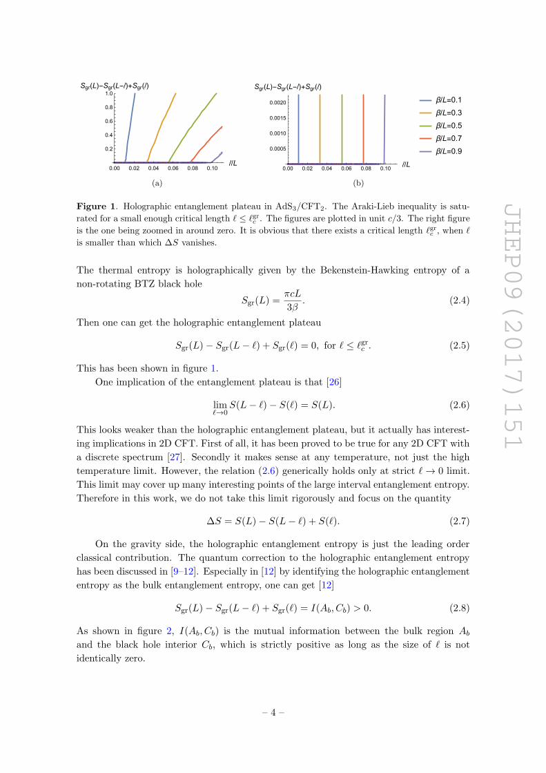
Figure 1. Holographic entanglement plateau in AdS3/CFT2. The Araki-Lieb inequality is satu-
rated for a small enough critical length ` ≤ `grc . The figures are plotted in unit c/3. The right figure
is the one being zoomed in around zero. It is obvious that there exists a critical length `grc , when `
is smaller than which ∆S vanishes.
The thermal entropy is holographically given by the Bekenstein-Hawking entropy of a
non-rotating BTZ black hole
Sgr(L) =πcL
3β. (2.4)
Then one can get the holographic entanglement plateau
One implication of the entanglement plateau is that [26]
lim`→0
S(L− `)− S(`) = S(L). (2.6)
This looks weaker than the holographic entanglement plateau, but it actually has interest-
ing implications in 2D CFT. First of all, it has been proved to be true for any 2D CFT with
a discrete spectrum [27]. Secondly it makes sense at any temperature, not just the high
temperature limit. However, the relation (2.6) generically holds only at strict `→ 0 limit.
This limit may cover up many interesting points of the large interval entanglement entropy.
Therefore in this work, we do not take this limit rigorously and focus on the quantity
∆S = S(L)− S(L− `) + S(`). (2.7)
On the gravity side, the holographic entanglement entropy is just the leading order
classical contribution. The quantum correction to the holographic entanglement entropy
has been discussed in [9–12]. Especially in [12] by identifying the holographic entanglement
entropy as the bulk entanglement entropy, one can get [12]
Sgr(L)− Sgr(L− `) + Sgr(`) = I(Ab, Cb) > 0. (2.8)
As shown in figure 2, I(Ab, Cb) is the mutual information between the bulk region Aband the black hole interior Cb, which is strictly positive as long as the size of ` is not
identically zero.
– 4 –
JHEP09(2017)151
AB AbBb Cb
(a)
AAbBBbCbC
(b)
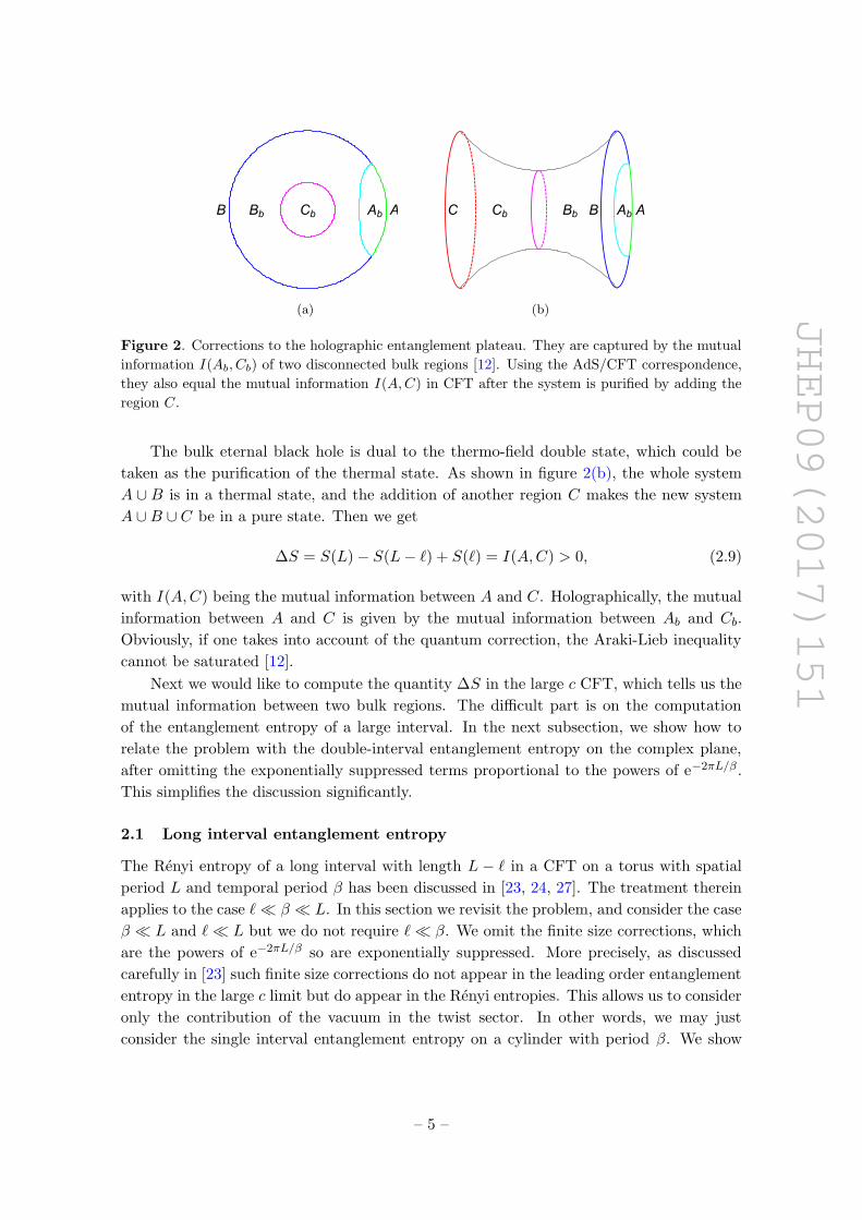
Figure 2. Corrections to the holographic entanglement plateau. They are captured by the mutual
information I(Ab, Cb) of two disconnected bulk regions [12]. Using the AdS/CFT correspondence,
they also equal the mutual information I(A,C) in CFT after the system is purified by adding the
region C.
The bulk eternal black hole is dual to the thermo-field double state, which could be
taken as the purification of the thermal state. As shown in figure 2(b), the whole system
A ∪ B is in a thermal state, and the addition of another region C makes the new system
A ∪B ∪ C be in a pure state. Then we get
∆S = S(L)− S(L− `) + S(`) = I(A,C) > 0, (2.9)
with I(A,C) being the mutual information between A and C. Holographically, the mutual
information between A and C is given by the mutual information between Ab and Cb.
Obviously, if one takes into account of the quantum correction, the Araki-Lieb inequality
cannot be saturated [12].
Next we would like to compute the quantity ∆S in the large c CFT, which tells us the
mutual information between two bulk regions. The difficult part is on the computation
of the entanglement entropy of a large interval. In the next subsection, we show how to
relate the problem with the double-interval entanglement entropy on the complex plane,
after omitting the exponentially suppressed terms proportional to the powers of e−2πL/β .
This simplifies the discussion significantly.
2.1 Long interval entanglement entropy
The Renyi entropy of a long interval with length L − ` in a CFT on a torus with spatial
period L and temporal period β has been discussed in [23, 24, 27]. The treatment therein
applies to the case `� β � L. In this section we revisit the problem, and consider the case
β � L and `� L but we do not require `� β. We omit the finite size corrections, which
are the powers of e−2πL/β so are exponentially suppressed. More precisely, as discussed
carefully in [23] such finite size corrections do not appear in the leading order entanglement
entropy in the large c limit but do appear in the Renyi entropies. This allows us to consider
only the contribution of the vacuum in the twist sector. In other words, we may just
consider the single interval entanglement entropy on a cylinder with period β. We show
– 5 –
JHEP09(2017)151
that the mutual information in (2.8), or equivalently in (2.9), equals the mutual information
of two intervals on the complex plane.
As shown in the left figure of figure 3, we consider the the long interval A = [−L/2, v]∪[u, L/2] with β � L and u − v = ` � L. Via the replica trick we need to compute the
partition function of the CFT on a Riemann surface Rn, which is obtained by pasting n
torus along the cuts. In the limits β � L, ` � L, the torus is approximately a cylinder
which we also denote by Rn, and for n = 1 it is an ordinary cylinder R. As shown in the
middle figure of figure 3, the cylinder Rn now is of length L and a temporal period nβ. We
use the coordinate w = x+ iτ on Rn. There are n cuts [v+ ijβ, u+ ijβ], j = 0, 1, · · · , n−1
with the same length u − v = ` in Rn, and the edges with the same color should be
identified. This is due to the fact that one may deform the interval on the torus [27]. The
original interval is very large, almost along the whole spatial direction of the torus. We
may take the interval to be the whole spatial direction minus the complement part, a short
interval of length `. The presence of the interval along the spatial direction is not trivial. It
induce the identification of the field in different replica such that the field theory is defined
on a cylinder with a temporal period nβ and n short cuts of length `. The Renyi entropy is
Sn(L− `) ≈ − 1
n− 1log
Z[Rn]
Z[R]n. (2.10)
In the above approximation, we have omitted the exponentially suppressed terms so that
the partition functions are defined on the cylinder. The Riemann surface Rn with coordi-
nate w can be mapped to an annulus with coordinate z by the conformal transformation
z = e2πwnβ . (2.11)
We denote the resulting annulus as Sn. The n cuts on Rn are mapped to the cuts on the
annulus along
[z(j)2 , z
(j)1 ] =
[e
2πvnβ
+ 2πijn , e
2πunβ
+ 2πijn
], j = 0, 1, · · · , n− 1. (2.12)
The boundaries of the cylinder at x = ±L/2 are mapped to the boundaries of the annulus
|z| = e±πLnβ . (2.13)
In the right figure of figure 3, we show the annulus Sn with n cuts, the edges of the same
color should be identified. We have the partition function
Z[Rn] = Z[Sn]. (2.14)
To regularize the ultra-violet(UV) divergences in the partition function and the Renyi
entropy, we have to impose cutoffs at the boundaries of the cuts in Rn and Sn. On Rn we
use the cutoff ε for every boundary, and so on Sn we have the cutoffs
2πε
nβz1,
2πε
nβz2, (2.15)
for the boundaries z(j)1 , z
(j)2 respectively.
– 6 –
JHEP09(2017)151
⇒ ⇒
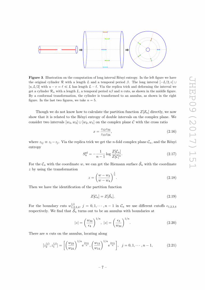
Figure 3. Illustration on the computation of long interval Renyi entropy. In the left figure we have
the original cylinder R with a length L and a temporal period β. The long interval [−L/2, v] ∪[u, L/2] with u− v = ` � L has length L− `. Via the replica trick and deforming the interval we
get a cylinder Rn with a length L, a temporal period nβ and n cuts, as shown in the middle figure.
By a conformal transformation, the cylinder is transformed to an annulus, as shown in the right
figure. In the last two figures, we take n = 5.
Though we do not know how to calculate the partition function Z[Sn] directly, we now
show that it is related to the Renyi entropy of double intervals on the complex plane. We
consider two intervals [w4, w3] ∪ [w2, w1] on the complex plane C with the cross ratio
x =z12z34
z13z24, (2.16)
where zij ≡ zi−zj . Via the replica trick we get the n-fold complex plane Cn, and the Renyi
entropy
Spln = − 1
n− 1log
Z[Cn]
Z[C]n. (2.17)
For the Cn with the coordinate w, we can get the Riemann surface Sn with the coordinate
z by using the transformation
z =
(w − w3
w − w4
) 1n
. (2.18)
Then we have the identification of the partition function
Z[Cn] = Z[Sn]. (2.19)
For the boundary cuts w(j)1,2,3,4, j = 0, 1, · · · , n − 1 in Cn we use different cutoffs ε1,2,3,4
respectively. We find that Sn turns out to be an annulus with boundaries at
|z| =(w34
ε4
)1/n
, |z| =(ε3w34
)1/n
. (2.20)
There are n cuts on the annulus, locating along
[z(j)2 , z
(j)1 ] =
[(w23
w24
)1/n
e2πijn ,
(w13
w14
)1/n
e2πijn
], j = 0, 1, · · · , n− 1, (2.21)
– 7 –
JHEP09(2017)151
⇒ ⇒
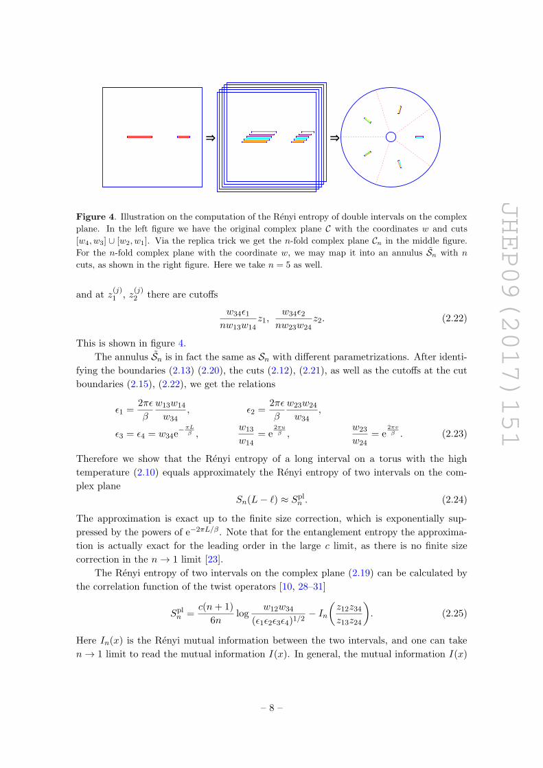
Figure 4. Illustration on the computation of the Renyi entropy of double intervals on the complex
plane. In the left figure we have the original complex plane C with the coordinates w and cuts
[w4, w3] ∪ [w2, w1]. Via the replica trick we get the n-fold complex plane Cn in the middle figure.
For the n-fold complex plane with the coordinate w, we may map it into an annulus Sn with n
cuts, as shown in the right figure. Here we take n = 5 as well.
and at z(j)1 , z
(j)2 there are cutoffs
w34ε1nw13w14
z1,w34ε2nw23w24
z2. (2.22)
This is shown in figure 4.
The annulus Sn is in fact the same as Sn with different parametrizations. After identi-
fying the boundaries (2.13) (2.20), the cuts (2.12), (2.21), as well as the cutoffs at the cut
boundaries (2.15), (2.22), we get the relations
ε1 =2πε
β
w13w14
w34, ε2 =
2πε
β
w23w24
w34,
ε3 = ε4 = w34e−πL
β ,w13
w14= e
2πuβ ,
w23
w24= e
2πvβ . (2.23)
Therefore we show that the Renyi entropy of a long interval on a torus with the high
temperature (2.10) equals approximately the Renyi entropy of two intervals on the com-
plex plane
Sn(L− `) ≈ Spln . (2.24)
The approximation is exact up to the finite size correction, which is exponentially sup-
pressed by the powers of e−2πL/β . Note that for the entanglement entropy the approxima-
tion is actually exact for the leading order in the large c limit, as there is no finite size
correction in the n→ 1 limit [23].
The Renyi entropy of two intervals on the complex plane (2.19) can be calculated by
the correlation function of the twist operators [10, 28–31]
Spln =
c(n+ 1)
6nlog
w12w34
(ε1ε2ε3ε4)1/2− In
(z12z34
z13z24
). (2.25)
Here In(x) is the Renyi mutual information between the two intervals, and one can take
n→ 1 limit to read the mutual information I(x). In general, the mutual information I(x)
– 8 –
JHEP09(2017)151
depends on the spectrum and the structure constants of the CFT. For a large c CFT, the
contributions are dominated by the those from the vacuum module. We review the results
in appendix A. Using the identifications (2.23), we get
Sn(L− `) ≈ c(n+ 1)
6nlog
(β
πεsinh
π`
β
)+πc(n+ 1)
6n
L
β− In
(1− e
− 2π`β
). (2.26)
Note that we need β, ` � L for the above approximation to be valid. When ` � β � L,
it is just
Sn(L− `) ≈ c(n+ 1)
6nlog
(β
πεsinh
π`
β
)+πc(n+ 1)
6n
L
β. (2.27)
and this is in accord to the holographic entanglement entropy (2.2) and the results
in [23, 24, 27]. When β � ` � L, the mutual information In in (2.26) gives an order
c contribution, which should be taken into account into the leading order contribution.
Finally we get
Sn(L− `) ≈ c(n+ 1)
6nlog
(β
πεsinh
π(L− `)β
), (2.28)
which is in accord to the holographic entanglement entropy (2.2).
It is remarkable that the treatment in this section has a larger validity domain than
that in [23, 24, 27]. An important simplification in our discussion is to omit the finite size
correction, which include the exponentially suppressed terms. This allows us to get the
result in the region β � `� L, which is beyond the one in the existing treatment.
Another remarkable fact is that the terms proportional to c in the entanglement en-
tropies are actually of universal form. They are either the single-interval Renyi entropy at
a finite temperature, or the Renyi entropy of the whole system. They are still true even
for a general 2D CFT.
2.2 Corrections to entanglement plateau
In the high temperature limit β � L, the entanglement entropy of a short interval with
`/L� 1 is approximately
Ssh(`) ≈ c
3log
(β
πεsinh
π`
β
). (2.29)
Taking n→ 1 limit of the result in the previous subsection we get the entanglement entropy
of a long interval
Slo(L− `) ≈ c
3log
(β
πεsinh
π`
β
)+πcL
3β− I
(1− e
− 2π`β
). (2.30)
For the large c CFT, if we only consider the leading contributions, then using (A.2) we get
Slo(`) =
c3 log β
2πε + cπ`3β when ` < L− `cft
c
c3 log
(βπε sinh π(L−`)
β
)+ πcL
3β when ` > L− `cftc ,
(2.31)
with the critical length
`cftc =
β
2πlog 2 (2.32)
which is the same as the gravity critical length `grc (2.3) in high temperature limit.
– 9 –
JHEP09(2017)151
0.2 0.4 0.6 0.8 1.0ℓ/L
2.×10-10
4.×10-10
6.×10-10
8.×10-10
1.×10-9
1.2×10⁻⁹
1.4×10⁻⁹
(a) β/L = 0.1
0.2 0.4 0.6 0.8 1.0ℓ/L
0.0005
0.0010
0.0015
0.0020
0.0025
0.0030
(b) β/L = 0.3
0.2 0.4 0.6 0.8 1.0ℓ/L
0.01
0.02
0.03
0.04
0.05
0.06
(c) β/L = 0.5
0.2 0.4 0.6 0.8 1.0ℓ/L
0.05
0.10
0.15
0.20
(d) β/L = 0.7
0.2 0.4 0.6 0.8 1.0ℓ/L
0.1
0.2
0.3
0.4
Ssh(ℓ)-Sgr(ℓ)
Slo(ℓ)-Sgr(ℓ)
(e) β/L = 0.9
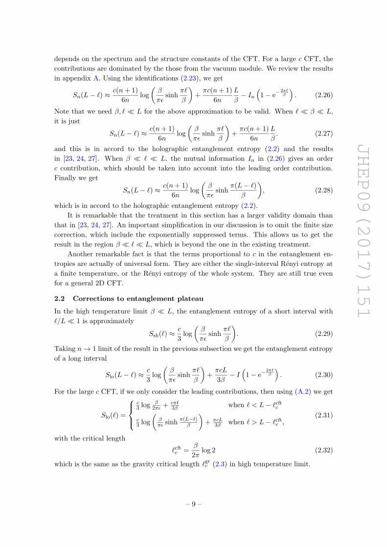
Figure 5. In the large c limit, the leading order entanglement entropy of a short interval (2.29)
and a long interval (2.31). We use the holographic entanglement entropy (2.2) as the benchmark
to compare. The figures are plotted in unit of c/3.
Although the short interval entanglement entropy (2.29) is derived with the assumption
`/L� 1, it has a much larger validity domain and matches the gravity result (2.2) as long
as 0 < ` < L−`c. The long interval entanglement entropy (2.31) is derived with assumption
(L − `)/L � 1, and it strictly matches the gravity result (2.2) for L − `c < ` < L, and
it also approximately matches (2.2) for β � ` < L. One can see this in figure 5. Note
that the short interval result (2.29) breaks down abruptly as `→ L, and and long interval
result (2.31) breaks down in a milder way as `→ 0.
Next we consider the next-to-leading order contribution to the entanglement entropies
of the long and the short intervals in the large c limit. We will see how such correction
change the entanglement plateau. First of all, for a CFT at a high temperature, omitting
the exponentially suppressed terms, one can easily get its thermal entropy
S(L) ≈ πcL
3β, (2.33)
which equals the black hole entropy (2.4). Then the correction to the entanglement
plateau is
∆S = S(L)− Slo(L− `) + Ssh(`) = I(
1− e− 2π`
β
)> 0, (2.34)
which is strictly positive as long as ` 6= 0. With the contributions from only the vacuum
module, we use (A.2), (A.3) and plot it in figure 6, and one can compare it with the gravity
result in figure 1.
There are other contributions to the mutual information from nonvacuum modules.
As we have shown, the function I(x) is actually related to the mutual information between
two intervals. The contribution from other modules can be read in a straightforward way.
In particular, as shown in [29, 32], the leading contribution from a primary module could
– 10 –
JHEP09(2017)151
0.00 0.02 0.04 0.06 0.08 0.10ℓ/L
0.2
0.4
0.6
0.8
1.0S(L)-Slo(L-ℓ)+Ssh(ℓ)
(a)
0.00 0.02 0.04 0.06 0.08 0.10ℓ/L
0.0005
0.0010
0.0015
0.0020
S(L)-Slo(L-ℓ)+Ssh(ℓ)β/L=0.1
β/L=0.2
β/L=0.3
β/L=0.5
β/L=0.7
β/L=0.9
(b)
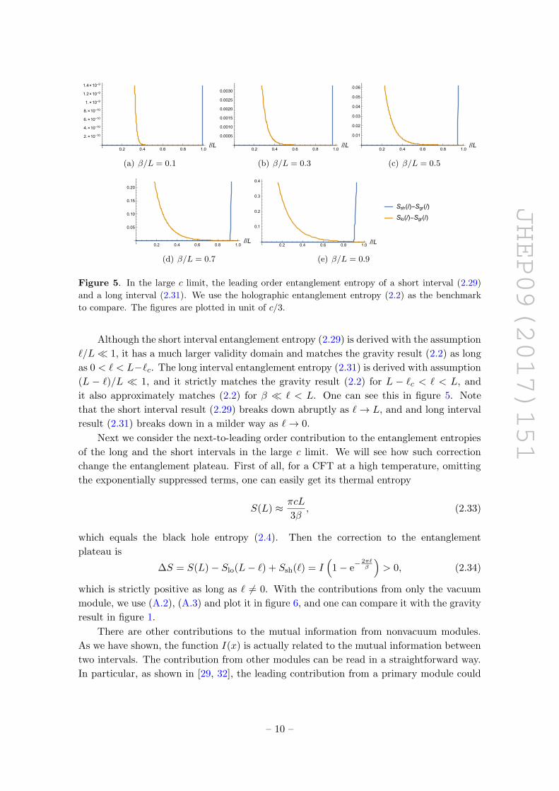
Figure 6. Corrections to the entanglement plateau in 2D CFT. We just set c = 3 to plot the
figures. From the left figure it seems suggest that the plateau is still there. The right figure shows
∆S after zooming in around the zero. From the right figure, it is easy to see that the plateau
disappears: ∆S = 0 only when l→ 0.
be of a universal form. As a result, when `� β, the correction from a nonvacuum module
with a primary operator X of scaling dimension ∆X takes a universal form so that we have
δX(S(L)− Slo(L− `) + Ssh(`)
)=
√πΓ(2∆X + 1)
4Γ(2∆X + 3/2)
(π`
β
)2∆X
+O(`2∆X+1, `3∆X ). (2.35)
Note that the universal contribution from the nonvacuum module is independent of the
central charge and the structure constants. For the contributions from the nonvacuum
modules, only the leading one from each module takes a universal form, while the subleading
ones rely on the details of the theory.
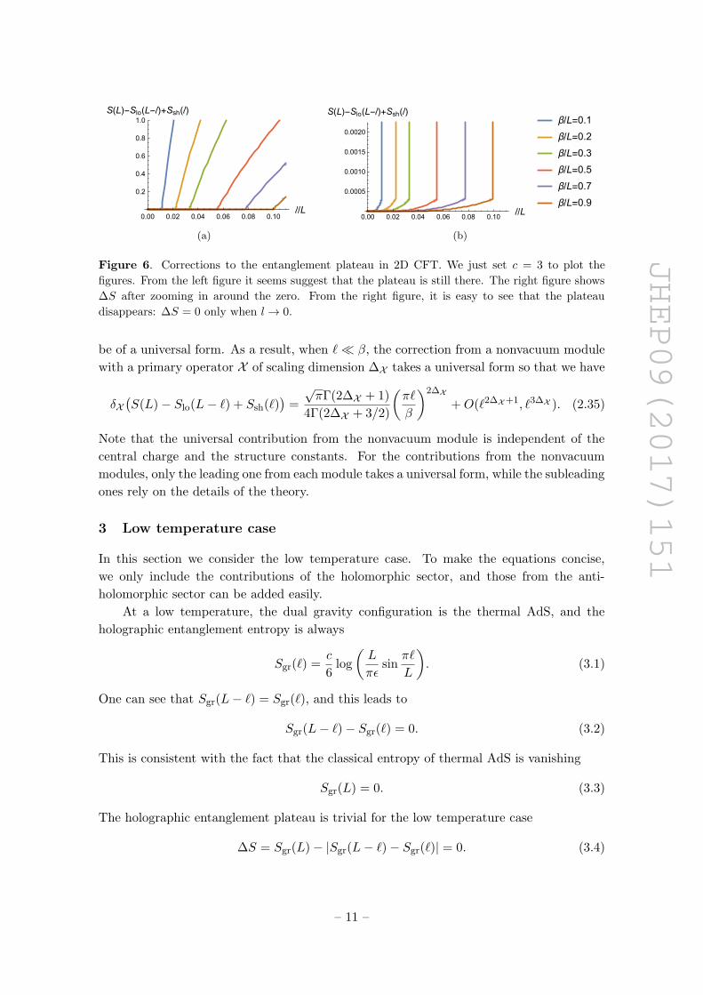
3 Low temperature case
In this section we consider the low temperature case. To make the equations concise,
we only include the contributions of the holomorphic sector, and those from the anti-
holomorphic sector can be added easily.
At a low temperature, the dual gravity configuration is the thermal AdS, and the
holographic entanglement entropy is always
Sgr(`) =c
6log
(L
πεsin
π`
L
). (3.1)
One can see that Sgr(L− `) = Sgr(`), and this leads to
Sgr(L− `)− Sgr(`) = 0. (3.2)
This is consistent with the fact that the classical entropy of thermal AdS is vanishing
Sgr(L) = 0. (3.3)
The holographic entanglement plateau is trivial for the low temperature case
∆S = Sgr(L)− |Sgr(L− `)− Sgr(`)| = 0. (3.4)
– 11 –
JHEP09(2017)151
AB AbBb
(a)
AAbBBbCbC
(b)
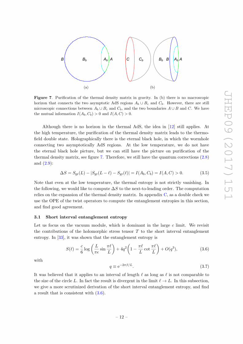
Figure 7. Purification of the thermal density matrix in gravity. In (b) there is no macroscopic
horizon that connects the two asymptotic AdS regions Ab ∪ Bc and Cb. However, there are still
microscopic connections between Ab ∪ Bc and Cb, and the two boundaries A ∪ B and C. We have
the mutual information I(Ab, Cb) > 0 and I(A,C) > 0.
Although there is no horizon in the thermal AdS, the idea in [12] still applies. At
the high temperature, the purification of the thermal density matrix leads to the thermo-
field double state. Holographically there is the eternal black hole, in which the wormhole
connecting two asymptotically AdS regions. At the low temperature, we do not have
the eternal black hole picture, but we can still have the picture on purification of the
thermal density matrix, see figure 7. Therefore, we still have the quantum corrections (2.8)
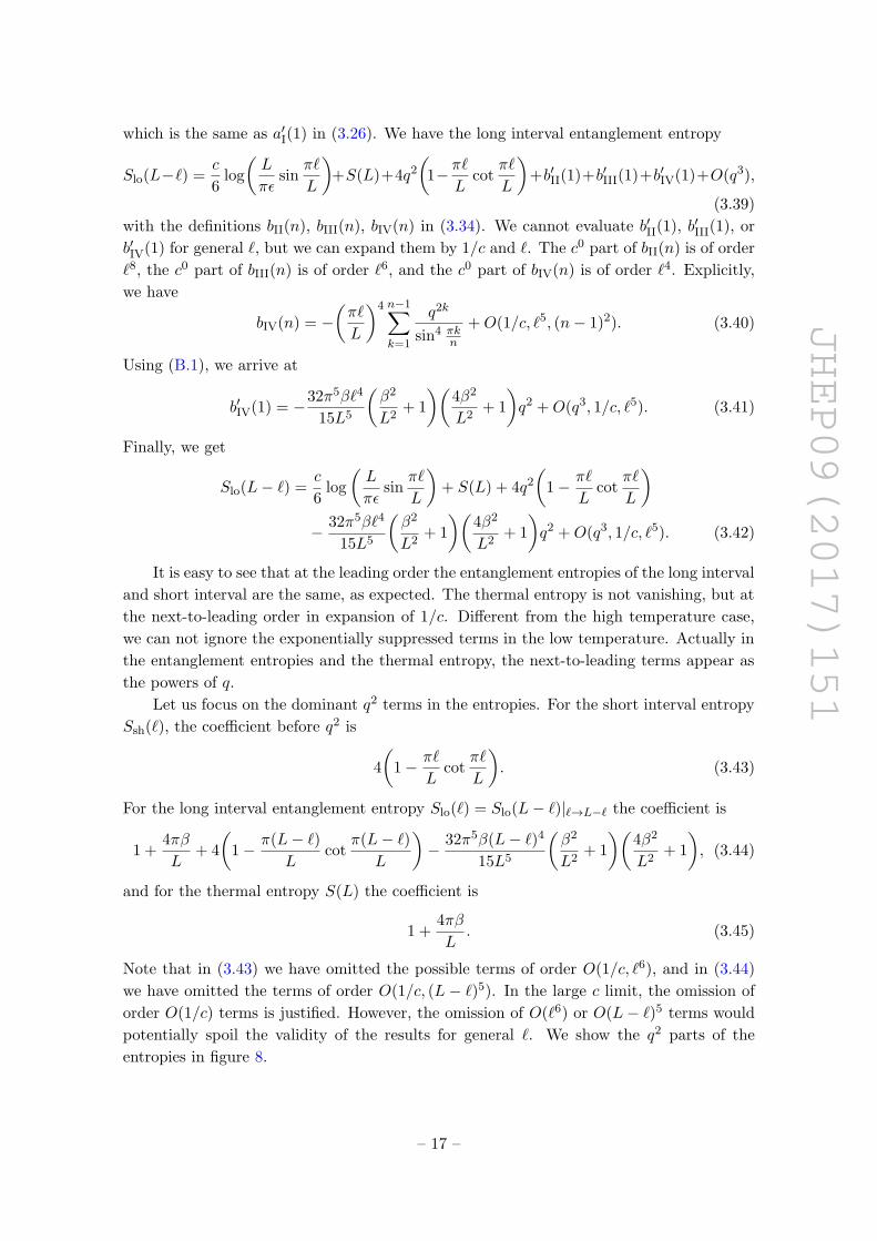
which is the same as a′I(1) in (3.26). We have the long interval entanglement entropy
Slo(L−`) =c
6log
(L
πεsin
π`
L
)+S(L)+4q2
(1− π`
Lcot
π`
L
)+b′II(1)+b′III(1)+b′IV(1)+O(q3),
(3.39)
with the definitions bII(n), bIII(n), bIV(n) in (3.34). We cannot evaluate b′II(1), b′III(1), or
b′IV(1) for general `, but we can expand them by 1/c and `. The c0 part of bII(n) is of order
`8, the c0 part of bIII(n) is of order `6, and the c0 part of bIV(n) is of order `4. Explicitly,
we have
bIV(n) = −(π`
L
)4 n−1∑k=1
q2k
sin4 πkn
+O(1/c, `5, (n− 1)2). (3.40)
Using (B.1), we arrive at
b′IV(1) = −32π5β`4
15L5
(β2
L2+ 1
)(4β2
L2+ 1
)q2 +O(q3, 1/c, `5). (3.41)
Finally, we get
Slo(L− `) =c
6log
(L
πεsin
π`
L
)+ S(L) + 4q2
(1− π`
Lcot
π`
L
)− 32π5β`4
15L5
(β2
L2+ 1
)(4β2
L2+ 1
)q2 +O(q3, 1/c, `5). (3.42)
It is easy to see that at the leading order the entanglement entropies of the long interval
and short interval are the same, as expected. The thermal entropy is not vanishing, but at
the next-to-leading order in expansion of 1/c. Different from the high temperature case,
we can not ignore the exponentially suppressed terms in the low temperature. Actually in
the entanglement entropies and the thermal entropy, the next-to-leading terms appear as
the powers of q.
Let us focus on the dominant q2 terms in the entropies. For the short interval entropy
Ssh(`), the coefficient before q2 is
4
(1− π`
Lcot
π`
L
). (3.43)
For the long interval entanglement entropy Slo(`) = Slo(L− `)|`→L−` the coefficient is
1 +4πβ
L+ 4
(1− π(L− `)
Lcot
π(L− `)L
)− 32π5β(L− `)4
15L5
(β2
L2+ 1
)(4β2
L2+ 1
), (3.44)
and for the thermal entropy S(L) the coefficient is
1 +4πβ
L. (3.45)
Note that in (3.43) we have omitted the possible terms of order O(1/c, `6), and in (3.44)
we have omitted the terms of order O(1/c, (L − `)5). In the large c limit, the omission of
order O(1/c) terms is justified. However, the omission of O(`6) or O(L− `)5 terms would
potentially spoil the validity of the results for general `. We show the q2 parts of the
entropies in figure 8.
– 17 –
JHEP09(2017)151
0.2 0.4 0.6 0.8 1.0ℓ/L
-5
5
10
15
20
25
30
0.981026 1
(a) β/L = 2
0.2 0.4 0.6 0.8 1.0ℓ/L
10
20
30
40
0.992446 1
(b) β/L = 3
0.2 0.4 0.6 0.8 1.0ℓ/L
20
40
60
0.998103 1
(c) β/L = 5
0.2 0.4 0.6 0.8 1.0ℓ/L
20
40
60
80
100
0.999245 1
(d) β/L = 7
0.2 0.4 0.6 0.8 1.0ℓ/L
-20
20
40
60
80
100
120
0.999523 1
q2 part of Ssh(ℓ)
q2 part of Slo(ℓ)
q2 part of S(L)
(e) β/L = 9
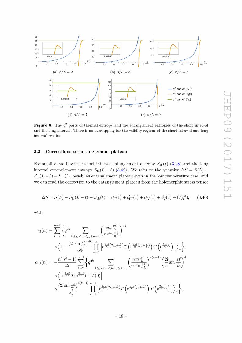
Figure 8. The q2 parts of thermal entropy and the entanglement entropies of the short interval
and the long interval. There is no overlapping for the validity regions of the short interval and long
interval results.
3.3 Corrections to entanglement plateau
For small `, we have the short interval entanglement entropy Ssh(`) (3.28) and the long
interval entanglement entropy Slo(L − `) (3.42). We refer to the quantity ∆S = S(L) −Slo(L− `) + Ssh(`) loosely as entanglement plateau even in the low temperature case, and
we can read the correction to the entanglement plateau from the holomorphic stress tensor
We expand the result (3.46) by small ` while keeping the central charge c general. It is
easy to see that cII(n), cIV(n) are of order `4, and cIII(n), cV(n) are of order `6. Explicitly,
we get
cII(n) = −4
c
(π`
L
)4 n−1∑k=2
Ck−2n−2q
2kn−1∑j=1
1
sin4 πjn
+O(`5, (n− 1)2),
cIV(n) =
(π`
L
)4 n−1∑k=1
q2k
sin4 πkn
+O(`5, (n− 1)2). (3.48)
Then we get the corrections to the entanglement plateau
S(L)−Slo(L−`)+Ssh(`) =32q2
15
(π`
L
)4[1
c+πβ
L
(β2
L2+1
)(4β2
L2+1
)]+O(q3, `5). (3.49)
Note that in the above result we do not require the central charge to be large, but we have
only incorporated the contributions from the vacuum module.
3.4 Low temperature case with nonvacuum module
In this subsection we consider the low temperature case with the leading contributions from
a holomorphic nonvacuum module. We consider the module with a general holomorphic
primary operator X of conformal weight hX and normalization αX . It was shown in [33]
the leading order correction to the single-interval entanglement entropy from the module
X takes a universal form
δXS(`) = 2hX qhX
(1− π`
Lcot
π`
L
)+O(qhX+1, q2hX ). (3.50)
It was believed that this applies to a general interval as long as the length ` cannot be
comparable to length of the system L.
Due to the presence of the primary module, we find that the corrections to the density
matrix and the reduced density matrices are respectively
δXρ =qhX
αX|X 〉〈X |+O(qhX+1), δXρA =
qhX
αXρA,X +O(qhX+1). (3.51)
– 19 –
JHEP09(2017)151
Using the same method as in subsection 3.1 we may get the corrections to the short interval
entanglement entropy
δXSsh(`) = 2hX qhX
(1− π`
Lcot
π`
L
)+ ∂na
IIX (n)|n=1 +O(qhX+1, q2hX ), (3.52)
with
aIIX (n) = −
n∑k=2
{qkhX
(sin π`
L
n sin π`nL
)2khX(1 + qhX
(sin π`
L
n sin π`nL
)2hX)n−k(3.53)
×∑
Z1,··· ,Zk
∑0≤j1<···<jk≤n−1
⟨ k∏a=1
[DXXZa
(e
2πinja(e
2πi`nL − 1
))hZaZa (e2πinja) ]⟩
C
}.
In aIIX (n) the quantities DXXZa are defined by the OPE of X (z1)X (z2)
FX (z1, z2) = 1 +∑Y
CXXYαXαY
∞∑r=0
arYr!
(z1 − z2)hY+r∂rY(z2)
= 1 +∑ZDXXZ(z1 − z2)hZZ(z2), (3.54)
with arY =CrhY+r−1
Cr2hY+r−1. The summation for Y runs over all the nonidentity holomorphic
quasiprimary operators with each Y being of conformal weight hY , and the summation
for Z runs over all the nonidentity holomorphic operators, including the quasiprimary
operators and their derivatives. It is possible that the term ∂naIIX (n)|n=1 give the same
order of contribution as qhX . It would be nice if ∂naIIX (n)|n=1 can be evaluated without
taking small ` expansion.
Similarly, we can read the correction to the thermal entropy and the entanglement
entropy of the long interval. The correction to the thermal entropy from the primary
module X is
δXS(L) =
(1 +
2πhXβ
L
)qhX +O(qhX+1, q2hX ). (3.55)
The corrections to the long interval entanglement entropy is
δXSlo(L− `) = (3.56)
δXS(L) + 2hX qhX
(1− π`
Lcot
π`
L
)+ ∂nb
IIX (n)|n=1 + ∂nb
IIIX (n)|n=1 +O(qhX+1, q2hX ),
– 20 –
JHEP09(2017)151
with the definitions
bIIX (n) = −qnhX(
sin π`L
n sin π`nL
)2nhX
(3.57)
×n∑k=2
∑Z1,··· ,Zk
∑0≤j1<···<jk≤n−1
⟨ k∏a=1
[DXXZa
(e
2πinja(e
2πi`nL − 1
))hZaZa (e2πinja) ]⟩
C,
bIIIX (n) = −n−1∑k=1
qkhX∑
0≤j1<···<jk≤n−1
(2in sin π`
L
)2khXαkX
×⟨ k∏a=1
[e
2πihXn (2ja+1− `
L)X(
e2πin (ja+1− `
L))X(
e2πinja) ]⟩
C.
The long interval result (3.56) is not universal and depends on the structure con-
stants, and the short interval result (3.52) is also possibly not universal. One can com-
pare (3.52), (3.56) with the result (3.50), which was obtained in [33]. We get the different
results by using a refined n → 1 limit. We sum all the terms of orders qhX , q2hX , · · · ,q(n−1)hX , qnhX before taking the n→ 1 limit, while in [33] only the term of order qhX was
kept in obtaining (3.50). Though it is fine to keep only the order qhX term in calculating
the n-th Renyi entropy with n = 2, 3, 4, · · · , we need to keep all the terms of orders qhX ,
q2hX , · · · , q(n−1)hX , qnhX to get the correct n → 1 limit. One justification for our treat-
ment is that δXS(`) in (3.50) is ill-defined in the limit `→ L while δXSlo(L− `) in (3.56)
is well-defined in the limit `→ 0. Note that it is still possible (3.50) is correct for a short
interval, i.e., that in (3.52) it is possible ∂naIIX (n)|n=1 ∼ O(q2hX ).
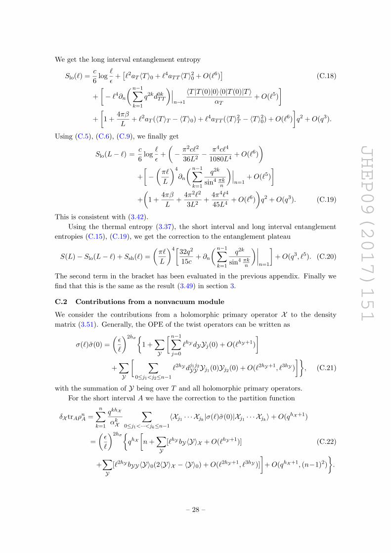
Summing up all the contributions, we find the correction to the entanglement plateau
The summation for Y runs over all the nonidentity holomorphic quasiprimary operators.
Finally we find
δX (S(L)− Slo(L− `) + Ssh(`))
=
√πqhX
4
∑Y
[C2XXY
α2XαY
Γ(hY + 1)
Γ(hY + 3/2)
(π`
L
)2hY
+O(`2hY+1, `3hY )
]
+
(π`
L
)2hX
∂n
[ n−1∑k=1
qkhX
(sin πkn )2hX
]∣∣∣n→1
+O(qhX+1, q2hX , `2hX+1). (3.61)
In the summation over Y, the holomorphic quasiprimary operator with the smallest con-
formal weight in each module dominates. For the vacuum module it is the stress tensor T ,
and for a nonvacuum module it is just the primary operator. The summation of Y in (3.61)
runs over T and all the nonidentity holomorphic primary operators. For the stress tensor,
it gives the correction (3.49). Note that that the result (3.61) does not take a universal
form, as it depends on the structure constants.
4 Conclusion and discussions
In this work, we studied the single-interval entanglement entropies at finite temperature in
2D CFT. We focused on the high temperature case with β � L and the low temperature
case with L� β. In particular we computed the entanglement entropies in the short and
large interval limits. This allows us to discuss the subleading correction to the entanglement
plateau
∆S = S(L)− |S(L− `)− S(`)| (4.1)
where S(L) is the thermal entropy of the system at the finite temperature. A general
lesson is that the Araki-Lieb inequality is robust and cannot be saturated for a finite ` if
the next-to-leading order contributions of large c limit are taken into account.
For the large c CFT with a gravity dual, it was found that there could be a holographic
entanglement plateau at a high temperature. As suggested in [12], ∆S is the mutual
information between the interior of the black hole and the region enclosed by the minimal
surface γ` [12]. We explicitly computed this mutual information in this work. In the semi-
classical AdS3/CFT2, we showed that ∆S is nonvanishing but is always an order c0 effect,
including both the contributions from the vacuum module and other primary modules.
In computing the entanglement entropies at a high temperature, we omitted the fi-
nite size effect, which contributes the exponentially suppressed terms. This simplifies the
– 22 –
JHEP09(2017)151
computation significantly and allows us to relate the computation with the computation
on the Renyi entropy of the two disconnected intervals on a complex plane. One impor-
tant consequence is that the leading contribution from the a nonvacuum module takes a
universal form.
On the other hand, in the low temperature case we cannot ignore the exponentially
suppressed terms. We used two different approaches to compute the thermal corrections
to the entanglement entropies and found consistent results. Quite interestingly we found
that the leading thermal correction to the long interval entanglement entropy actually does
not take a universal form. Instead, the leading correction to entanglement plateau actually
depends on the details of the theory.
It is remarkable that our treatment in this work does not restrict to the large c CFT,
and can be applied to a general CFT. In 2D CFT, the vacuum module is special as it
includes the stress tensor which encodes the information on the central charge. Therefore
the discussion on the vacuum module in this work certainly applies to other CFTs. At
the high temperature the case is related to the double interval mutual information on the
complex plane. In the latter case the leading contribution of the nonvacuum module to the
mutual information is of universal form. At the low temperature, the picture is similar but
the leading contributions from nonvacuum modules depend on the details of the theory.
Simply speaking, in a general 2D CFT the corrections from both vacuum and nonvacuum
modules are not suppressed by 1/c and so the entanglement plateau disappears.
Acknowledgments
We thank Peng-xiang Hao for a partial collaboration on this work, especially the calculation
in appendix C. We thank Erik Tonni for helpful discussions. We thank the Galileo Galilei
Institute for Theoretical Physics for the hospitality and the INFN for partial support during
the completion of this work. BC would like to thank Centro de Ciencias de Benasque Pedro
Pascual for hospitality during the completion of this work. BC was in part supported by
NSFC Grant No. 11275010, No. 11335012 and No. 11325522. ZL was supported by NSFC
Grant No. 11575202. JJZ was supported by the ERC Starting Grant 637844-HBQFTNCER
and in part by Italian Ministero dell’Istruzione, Universita e Ricerca (MIUR) and Istituto
Nazionale di Fisica Nucleare (INFN) through the “Gauge Theories, Strings, Supergravity”
(GSS) research project.
A Mutual information of two intervals on a complex plane
Here we review the useful property of the mutual information I(x) between two intervals
in a large c CFT with contributions from the vacuum module [10, 11, 29–31, 36, 37]. The
mutual information can be organized by orders of c
I(x) = IL(x) + INL(x) + · · · , (A.1)
– 23 –
JHEP09(2017)151
where x is the cross ratio. The leading part of the mutual information is universal and do
not depend on the details of the CFT
IL(x) =
{0 when x < 1/2c3 log x
1−x when x > 1/2,(A.2)
and with contributions of only the vacuum module the next-to-leading part can be written
in expansion of small x
INL(x) =x4
630+
2x5
693+
15x6
4004+
x7
234+
167x8
36036+
69422x9
14549535+
122x10
24871+O(x11). (A.3)
One has [10]
INL(x) = INL(1− x). (A.4)
For a nonvacuum module with a primary operator X of the scaling dimension ∆X , there
is a universal correction at the leading order [29]
δX I(x) =
√πΓ(2∆X + 1)x2∆X
42∆X+1Γ(2∆X + 3/2)+O(x2∆X+1, x3∆X ). (A.5)
In fact, for any 2D CFT the small x expansion of the mutual information can be
written as [36, 37]
I(x) = limn→1
1
n− 1
∑K
αKd2Kx
hK+hK2F1(hK , hK ; 2hK ;x)2F1(hK , hK ; 2hK ;x), (A.6)
where the summation K runs over all orthogonalized quasiprimary operators ΦK , with
conformal weights (hK , hK) and normalization αK , in the n-fold CFT that we call CFTn,
and dK is the OPE coefficient of twist operators. It is just (A.3) with the contributions
from only the vacuum module. The leading contribution from a nonvacuum module takes
the universal form (A.5), while the subleading contributions are not universal and depend
on details of the CFT. Also the subleading contributions from different modules are mixed
and cannot be separated.
B Analytical continuation
In the appendix, we prove the following identity2
∂n
( n−1∑k=1
q2k
sin4 πkn
)∣∣∣n=1
=32πβ
15L
(β2
L2+ 1
)(4β2
L2+ 1
)q2 +O(q3). (B.1)
Note that q = e−2πβ/L.
We consider the Mellin transform and its inverse transform
F (s) =
∫ ∞0
f(x)xs−1dx,
f(x) =1
2πi
∫ c+i∞
c−i∞F (s)x−sds. (B.2)
2We thank Peng-xiang Hao for his contributions to this appendix.
– 24 –
JHEP09(2017)151
We choose
F (s) =1
[sin(πs)]4, (B.3)
and so
f(x) =(log x)3 + 4π2 log x
6π4(x− 1). (B.4)
Then we getn−1∑k=1
q2k
sin4 πkn
=
∫ ∞0
q2x1/n − q2nx
x(1− q2x1/n)f(x)dx, (B.5)
which leads to
∂n
( n−1∑k=1
q2k
sin4 πkn
)∣∣∣n=1
=
∫ ∞0
q2[log(q2) + log x]
q2x− 1f(x)dx. (B.6)
The integral on the right-hand side is convergent for Req2 ≤ 0, Imq2 6= 0, and with an
analytical continuation we finally get
∂n
( n−1∑k=1
q2k
sin4 πkn
)∣∣∣n=1
=q2 log(q2)[log(q2) + 4π2][log(q2) + 16π2]
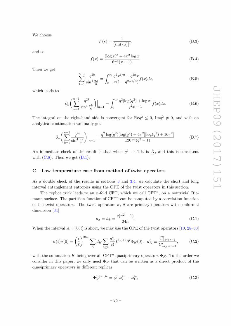
120π4(q2 − 1). (B.7)
An immediate check of the result is that when q2 → 1 it is 815 , and this is consistent
with (C.8). Then we get (B.1).
C Low temperature case from method of twist operators
As a double check of the results in sections 3 and 3.4, we calculate the short and long
interval entanglement entropies using the OPE of the twist operators in this section.
The replica trick leads to an n-fold CFT, which we call CFTn, on a nontrivial Rie-
mann surface. The partition function of CFTn can be computed by a correlation function
of the twist operators. The twist operators σ, σ are primary operators with conformal
dimension [34]
hσ = hσ =c(n2 − 1)
24n. (C.1)
When the interval A = [0, `] is short, we may use the OPE of the twist operators [10, 28–30]
σ(`)σ(0) =
(ε
`
)2hσ∑K
dK∑r≥0
arKr!`hK+r∂rΦK(0), arK ≡
CrhK+r−1
Cr2hK+r−1
, (C.2)
with the summation K being over all CFTn quasiprimary operators ΦK . To the order we
consider in this paper, we only need ΦK that can be written as a direct product of the
quasiprimary operators in different replicas
Φj1j2···jkK = φj11 φ
j22 · · ·φ
jkk , (C.3)
– 25 –
JHEP09(2017)151
where 0 ≤ ji ≤ n − 1 labels the replica. From the OPE coefficients dj1j2···jkK for Φj1j2···jkK ,
we may define
bK =∑
j1,j2,··· ,jk
dj1j2···jkK , aK = − limn→1
bKn− 1
. (C.4)
For the vacuum module, we only need the quasiprimary operators Tj , Aj , Tj1Tj2 , with
0 ≤ j ≤ n− 1, 0 ≤ j1 < j2 ≤ n− 1, the corresponding dK can be found in [29–31], and the
corresponding bK can be found in [38, 39], from which we may get
aT = −1
6, aA = 0, aTT = − 1
30c. (C.5)
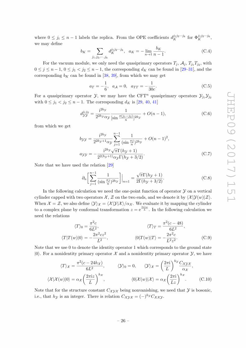
For a quasiprimary operator Y, we may have the CFTn quasiprimary operators Yj1Yj2with 0 ≤ j1 < j2 ≤ n− 1. The corresponding dK is [29, 40, 41]
dj1j2YY =i2hY
22hYαY
1
[sin π(j1−j2)n ]2hY
+O(n− 1), (C.6)
from which we get
bYY =i2hY
22hY+1αY
n−1∑j=1
1
(sin πjn )2hY
+O(n− 1)2,
aYY = − i2hY√πΓ(hY + 1)
22(hY+1)αYΓ(hY + 3/2). (C.7)
Note that we have used the relation [29]
∂n
[ n−1∑j=1
1
(sin πjn )2hY
]∣∣∣n=1
=
√πΓ(hY + 1)
2Γ(hY + 3/2). (C.8)
In the following calculation we need the one-point function of operator Y on a vertical
cylinder capped with two operators X , Z on the two ends, and we denote it by 〈X |Y(w)|Z〉.When X = Z, we also define 〈Y〉X = 〈X |Y|X 〉/αX . We evaluate it by mapping the cylinder
to a complex plane by conformal transformation z = e2πiwL . In the following calculation we
need the relations
〈T 〉0 =π2c
6L2, 〈T 〉T =
π2(c− 48)
6L2,
〈T |T (w)|0〉 = −2π2cz2
L2, 〈0|T (w)|T 〉 = − 2π2c
L2z2. (C.9)
Note that we use 0 to denote the identity operator 1 which corresponds to the ground state
|0〉. For a nonidentity primary operator X and a nonidentity primary operator Y, we have
〈T 〉X =π2(c− 24hX )
6L2, 〈Y〉0 = 0, 〈Y〉X =
(2πi
L
)hY CXYXαX
,
〈X |X (w)|0〉 = αX
(2πiz
L
)hX, 〈0|X (w)|X 〉 = αX
(2πi
Lz
)hX. (C.10)
Note that for the structure constant CXYX being nonvanishing, we need that Y is bosonic,
i.e., that hY is an integer. There is relation CXYX = (−)hYCXXY .
– 26 –
JHEP09(2017)151
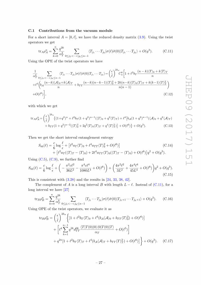
C.1 Contributions from the vacuum module
For a short interval A = [0, `], we have the reduced density matrix (3.9). Using the twist


![Published for SISSA by Springer2017)067.pdfposal of twistor string theory [10] and the resulting formula for gauge theory scattering amplitudes in four space-time dimensions [11],](https://static.documents.pub/doc/80x56/5ed94811a8e2071d2a5adc81/published-for-sissa-by-springer-2017067pdf-posal-of-twistor-string-theory-10.jpg)


