Pulsed Nuclear Magnetic Resonance: Spin Echoes

MIT Department of Physics

This experiment explores nuclear magnetic resonance (NMR) both as a physical phenomenon concerning atomic nuclei and as a ubiquitous laboratory technique for exploring the structure of bulk substances. Using radio frequency bursts tuned to resonance, pulsed NMR perturbs a thermal spin ensemble, which behaves on average like a magnetic dipole. One immediate consequence is the ability to measure the magnetic moments of certain nuclei such as hydrogen (i.e., the proton) and flourine; the former is of particular interest to nuclear physics.

In addition, the use of techniques like spin echoes lead to a myriad of pulse sequences which allow the determination of spin-lattice and spin-spin relaxation times of substances. Among the samples available in this lab are glycerin and paramagnetic ion solutions, whose viscocity and concentration strongly affect their relaxation times. Investigation of these dependences illustrate the use of pulsed NMR as a method for identifying and characterizing substances.

PREPARATORY QUESTIONS

Please visit the Pulsed NMR chapter on the course website to review the background material for this experiment. Answer all questions found in the chapter. Work out the solutions in your laboratory notebook; submit your answers on the website. [Note: Not available to OCW users.]

PROGRESS CHECK

By the end of your 2nd session in lab you should have a determination of the nuclear magnetic moment of fluo-rine. You should also have a preliminary value of T2 for 100% glycerine.

I. BACKGROUND

The NMR method for measuring nuclear magnetic mo-ments was conceived independently in the late 1940s by Felix Bloch and Edward Purcell, who were jointly awarded the Nobel Prize in 1952 for their work [1–4] Both investigators, applying somewhat different tech-niques, developed methods for determining the magnetic moments of nuclei in solid and liquid samples by mea-suring the frequencies of oscillating electromagnetic fields that resonantly induced transitions among their magnetic substates, resulting in the transfer of energy between the sample of the measuring device. Although the amounts of energy transferred are extremely small, the fact that the energy transfer is a resonance phenomenon enabled it to be measured. Bloch and Purcell both irradiated their samples with a

continuous wave (CW) of constant frequency while simul-taneously sweeping the magnetic field through the reso-nance condition. CW methods are rarely used in modern NMR experiments. Rather, radiofrequency (RF) energy is usually applied in the form of short bursts of radiation (hence, the term ”pulsed NMR”), and the effects of the induced energy level transitions are observed in the time

between bursts. More important, as we shall see, the techniques of pulsed NMR make it much easier to sort out the various relaxation effects in NMR experiments. Nevertheless, this experiment demonstrates the essen-

tial process common to all NMR techniques: the detec-tion and interpretation of the effects of a known perturba-tion on a system of magnetic dipoles embedded in a solid or liquid. As we shall see, this analysis of the system’s response to what is essentially a macroscopic perturba-tion yields interesting information about the microscopic structure of the material.

II. THEORY

II.1. Free Induction of a Classical Magnetic Moment

In classical electromagnetism, a charged body with nonzero angular momentum L possesses a quantity called a magnetic moment µ, defined by

µ = γL, (1)

where γ is the body’s gyromagnetic ratio, a constant depending on its mass and charge distribution. For a classical, spherical body of mass m and charge q dis-tributed uniformly, the gyromagnetic ratio is given by

qγcl = . (2)

2m

The magnetic moment is an interesting quantity be-cause when the body is placed in a static magnetic field B0, it experiences a torque

dL = µ × B0. (3)

dt

This equation of motion implies that if there is some nonzero angle α between L and B0, its axis of rotation L precesses about B0 at the rate

Id: 12.nmr.tex,v 1.117 2014/10/17 17:36:57 spatrick Exp ldana

2 Id: 12.nmr.tex,v 1.117 2014/10/17 17:36:57 spatrick Exp ldana

ωL = −γclB0 (4)

independently of the value of α, much like the behavior of a gyroscope in a uniform gravitational field. The mi-nus sign indicates that for a body with positive γ (e.g., positively charged sphere), the precession is clockwise. This phenomenon is called Larmor precession, and we call ωL =| ωL | the Larmor frequency. Suppose B0 = B0z; in this case, the x-y plane is

called the transverse plane. Next, suppose we place a solenoid around the magnetic moment, with the axis of the solenoid in the transverse plane (e.g., aligned with x). If α is nonzero, there is a nonzero transverse compo-nent of µ, which generates an oscillating magnetic field at the Larmor frequency. By Faraday’s law, this transverse component induces an emf

V (t) = V0(α)cos(ωLt + φ0). (5)

The phase φ0 is simply the initial transverse angle be-tween the µ and the solenoid axis, while V0 is an overall factor that incorporates constants like the overall magni-tudes of µ, signal amplification, and solenoid dimensions. It is worth noting, however, that V0 is a function of α: when α is zero, there is no signal, and as α is moved to-wards π/2, the signal reaches a maximum when µ lies in the transverse plane, which then decreases back to zero at α = π when µ is antiparallel to B0, and so on. But regardless of its magnitude, the induced emf al-

ways oscillates at the characteristic Larmor frequency. We call this detected voltage oscillation the free induc-tion NMR signal. It is this signal with which NMR is pri-marily concernedwe manipulate the magnetic moment of a sample and monitor the behavior of the free induction signal to understand its bulk material properties.

II.2. Nuclear Magnetism

In quantum mechanics, it is a fact that particles (i.e., electrons, protons, and composite nuclei) possess an in-trinsic quantity of angular momentum known as spin, which cannot quite be understood as any form of classical rotation. The particle’s spin angular momentum along any given direction is quantized, andfor a spin − 1 parti-2 cletakes on the values of +~/2 and −~/2, corresponding to two states we usually refer to as ”spin-up” and ”spin-down”. The general state (wavefunction) of any such two-state system is a complex superposition of these two eigenstates. We sketch a rough picture below of how macroscopic nuclear magnetism comes out of this micro-scopic framework; for more accurate details, see [5, 6]. There is no reason we should expect such a system

to behave anything like a classical particle with angular momentum. Yet, as shown in Appendix A, the wave-function for any two-state system can be visualized as a

vector in the Bloch sphere, using the relative phases in the superposition as direction angles. And it turns out that in this picture, when a charged quantum spin such as an atomic nucleus is placed in a static magnetic field, the wavefunction does indeed exhibit an analogue of Lar-mor precession in the Bloch sphere. Of course, there are key differences. For one thing, the precession frequency is not the same, owing to quantum effects. The difference is captured by changing the gyromagnetic ratio:

γ = gγcl. (6)

This corrective g-factor is analogous to the Lande g-factor in atomic spectroscopy and varies from nuclei to nuclei. We retain the definition of the magnetic mo-ment, so that in an eigenstate of angular momentum, the magnitude of the magnetic moment in that direction is µ = γ~/2. More significantly, however, precession of the wave-

function in the Bloch sphere is not quite the same as a precession in real space. For example, with a classi-cal magnetic moment µ aligned at some nonzero angle α with z, it is possible to measure precisely both µx = µ · xand µz = µ · z. But Heisenberg’s uncertainty principle forbids simultaneous measurements of both quantum op-erators and µx, µz even though the wavefunction vector in the Bloch sphere has well-defined projections onto x and z. Nevertheless, the expectation of the quantum magnetic

moment does behave exactly like the classical magnetic moment, in the limit of a large number of repeated mea-surements (a case of Ehrenfest’s theorem). It is precisely this correspondence that NMR relies on. But rather than making repeated measurement of a single quantum spin, we make an ensemble measurement of a large number of spins at once. If their wavefunctions are approximately the same (i.e., the spins are ”coherent”), then the en-semble should exhibit a macroscopic, classical magnetic moment. More precisely, what we measure in NMR is M = N

h µ i , or the expectation of the quantum magnetic mo-ment averaged over the bulk ensemble, multiplied by the number of spins which are coherent. Since the volume of our sample is fixed, this is proportional to the magnetiza-tion, and we will simply refer to M as the ”magnetization vector” of the sample. Our conclusion is that M exhibits the exact same dynamics as the classical magnetic mo-ment µ , generating an NMR free induction signal at the Larmor frequency ωL = γB0. It is worth noting that this macroscopic ensemble does indeed capture the quantum nature of the spins, by way of the non-classical gyromag-netic ratio γ.

II.3. Pulsed NMR

As suggested in Problem 3, the equilibrium state for a system of spins in a static magnetic field B0 = B0z

3 Id: 12.nmr.tex,v 1.117 2014/10/17 17:36:57 spatrick Exp ldana

produces a small magnetization M0 = M0z in the same direction as the magnetic field. However, we also know that such a configuration in which α = 0 still does not result in a free induction signal. We also need a way of perturbing the spins out of equilibrium, to generate a transverse component of the magnetization. We use a method called pulsed NMR in order to achieve this. In pulsed NMR, the same solenoid that is used to pick

up a transverse magnetization can also be used to gen-erate an RF field around the sample. We focus on the generation of a magnetic field

B1(t) = B1 cos ωtx (7)

It is standard to take B1 << B0, so that the field B1

can be treated as a perturbation. We then proceed to examine the behavior of M in response to this perturbing field. We first note that we can write B1 as a superposition

of two counter-rotating magnetic fields:

B1Br(t) = (cos ωtx+ sin ωty) (8)

2

B1Bl(t) = (cos ωtx+ sin ωty) (9)

2

Thus, B1 = Br + Bl. For nuclei with positive gyro-magnetic ratio, Bl rotates in the same direction as the magnetization (clockwise), while Br rotates in the oppo-site direction (counter-clockwise). We now consider the situation from the point of view of

an observer in a reference frame rotating in the direction of precession (that is, clockwise) with angular velocity ω. The unit vectors in this rotating frame are

x0 = cos ωtx− sin ωty (10)

y0 = sin ωtx− cos ωty (11)

z0 = z (12)

A moment’s thought will confirm that in the x y coor-dinate system, the x0 y0 system is indeed rotating clock-wise with angular velocity ω. In this rotating frame, the field Bl appears to be

stationary, while Br appears to be rotating counter-clockwise at a rate 2ω. This can be shown directly by solving for x and y in terms of x0 and y0 in the equa-tions above and substituting. The result is that the two rotating components become

B1Br = (cos 2ωtx0 + sin 2ωty0) (13)

2

1 Bl = Blx0 (14)

2

On the other hand, the static magnetic field does not appear any different, and B0 = B0x0. The total magnetic field in the rotating frame is, of

course, B = B0 +B1. But this magnetic field shouldeven in the rotating frameinduce a Larmor precession. The precession angular velocity of the magnetization vector in this frame is

Ω = −γB + ωz0 (15)

where the extra term comes from the kinematic mo-tion of the rotating frame (as if there were a fictitious magnetic field opposing B0 ). Written more explicitly in terms of components, we have

γB1 γB1Ω · x0 = − − cos 2ωt (16)

2 2

γB1Ω · y0 = − sin 2ωt (17)

2

Ω · z0 = −γB0 + ω (18)

Now the crucial point: when the frequency of the per-turbing field satisfies ω = γB0 = ωL (on resonance with the natural Larmor frequency), the rapid precession due to B0 vanishes in the rotating frame, and all that remains is a constant, slow precession about x0 at the rate γB1/2, with only the addition of tiny time-dependent flutters (the sines and cosines), which average out to zero. If M is initially parallel to B0, then application of the

perturbing pulse B1 for a time

π t90 = (19)

γB1

evidently rotates M by 90◦ about x0, placing M in the transverse plane perpendicular to B0. If the pulse is now turned off, M is left in the transverse plane, and from the point of view of an observer in the laboratory frame, it will be precessing at the Larmor frequency γB0 about z. By a similar argument, application of the perturbing pulse for a time t180 = 2t90 rotates M by 180◦, inverting the spin population. In practice, the value of 1 is not well-known, so t90 is usually found by trial and error, usually by looking for the pulse width which yields the greatest transverse magnetization.

II.4. Relaxation

Owing to the microscopic nature of nuclear magnetism, the free induction signal does not persist for very long.

4 Id: 12.nmr.tex,v 1.117 2014/10/17 17:36:57 spatrick Exp ldana

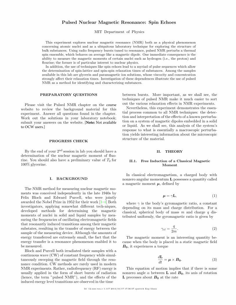
FIG. 1. An idealized scope trace of a free induction decay signal, showing also the decay envelope. The thick black line indicates the 90◦ perturbing pulse that puts the magnetiza-tion into the transverse plane. The decay constant T2

∗ consists of both the T2 effect discussed below as well as the effect of field inhomogeneities (discussed next section). Due to the latter effect, T2

∗ >> T1 in the real NMR setup.

Once perturbed, the spins proceed to return towards equilibrium, in a process called relaxation. Relaxation is one of the keys to the utility of NMR: different sub-stances return to equilibrium at different rates and in different ways; analysis of the relaxation times of a sam-ple gives significant insight into its chemical composition and structure. Relaxation mechanisms (and other effects, as discussed

in the following section) result in an exponential decay in the free induction NMR signal, which manifests itself as the ubiquitous free induction decay (FID) signal, a sketch of which is shown below. There are two relaxation mechanisms which are of

physical interest in this lab. The first is the eventual recovery of longitudinal magnetization (that is, magneti-zation along B0 ), due to rethermalization of the system. The second, which occurs even in the absence of the first, is the loss of transverse magnetization due to decoherence of the spins. Both of these mechanisms contribute to the decay observed in the FID, and the rates at which they occur depend on the substance in question. The first mechanism is typically called spin-lattice re-

laxation and the time constant governing its rate is de-noted T1. Its name derives from the fact that rethermal-ization is caused by the redistribution of energy from the spins to their surrounding environment (the ”lattice”). This has the effect of dissipating the energy of the pulse until the entire sample has returned to its original ther-mal state. If we use a 90◦ pulse to send the magnetization into the transverse plane at t = 0, then the spin-lattice relaxation process can be described by saying Mz recov-ers according to

−t/T1 ),Mz(t) = M0(1 − e (20)

where M0 is the magnitude of the longitudinal mag-

netization at thermal equilibrium. Of course, as Mz re-covers, the transverse magnetization correspondingly de-creases. The second mechanism is typically called spin-spin re-

laxation and the time constant governing its rate is de-noted T2. Its name derives from the idea that, as the spins are precessing, they feel small fluctuations in the magnetic field from magnetic dipole interactions of neigh-boring spins (perhaps other nuclei on the same molecule), which leads to randomization of the spin’s precessional motion. This causes the spinswhich were initially precess-ing in phase and constructively contributing to the trans-verse magnetizationto decohere and begin destructively interfering, diminishing the observed transverse magne-tization. This spin-spin relaxation process, like the spin-lattice relaxation, is an irreversible process, and it can be described by saying that the transverse magnetization Mxy decays according to

−t/T2Mxy(t) = M0e (21)

where M0 is the initial transverse magnetization at t = 0 right after a 90◦ pulse. Most of the measurement techniques used in this lab

center on the goal of obtaining these relaxation times for various substances. In particular, we are interested in how these relaxation times change as we vary the prop-erties of the substance such as concentration or viscos-ity. Typically, experiments to determine T1 perturb the system, let it relax, and then attempt to measure the re-covered longitudinal magnetization. On the other hand, experiments to find T2 rely on making observations of how the FID signal decays.

II.5. Spin Echoes

Although we are primarily interested in relaxation, there are other effects that contribute to the decay in the FID. The most important of these is inhomogene-ity in the magnetic field. A global inhomogeneity in the static magnetic field B0 can cause parts of the sample to precess at different rates, leading to phase differences and a loss of the ensemble-averaged transverse magneti-zation much more quickly than would be expected from just spin-spin interactions alone. In fact, for simple NMR setups such as the one used in

this lab where the static magnetic field is maintained by permanent magnets, such field inhomogeneities dominate relaxation. The observed decay constant of the FID is typically denoted T2

∗, and it consists of two components:

1/T ∗ = 1/T2 + γΔH0, (22)2

where T2 is the spin-spin relaxation time and ΔH0 is a measure of the inhomogeneity of the magnetic field over the sample volume.

5 Id: 12.nmr.tex,v 1.117 2014/10/17 17:36:57 spatrick Exp ldana

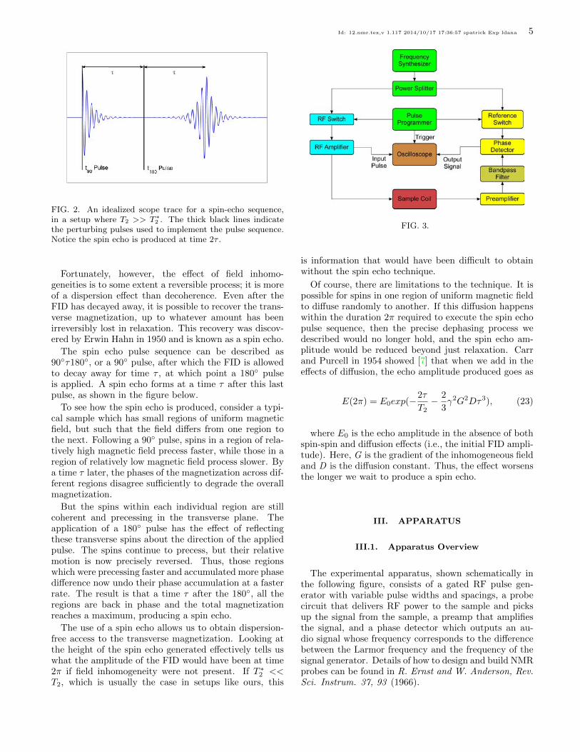
FIG. 2. An idealized scope trace for a spin-echo sequence, in a setup where T2 >> T 2

∗ . The thick black lines indicate the perturbing pulses used to implement the pulse sequence. Notice the spin echo is produced at time 2τ .

Fortunately, however, the effect of field inhomo-geneities is to some extent a reversible process; it is more of a dispersion effect than decoherence. Even after the FID has decayed away, it is possible to recover the trans-verse magnetization, up to whatever amount has been irreversibly lost in relaxation. This recovery was discov-ered by Erwin Hahn in 1950 and is known as a spin echo. The spin echo pulse sequence can be described as

90◦τ 180◦, or a 90◦ pulse, after which the FID is allowed to decay away for time τ , at which point a 180◦ pulse is applied. A spin echo forms at a time τ after this last pulse, as shown in the figure below. To see how the spin echo is produced, consider a typi-

cal sample which has small regions of uniform magnetic field, but such that the field differs from one region to the next. Following a 90◦ pulse, spins in a region of rela-tively high magnetic field precess faster, while those in a region of relatively low magnetic field process slower. By a time τ later, the phases of the magnetization across dif-ferent regions disagree sufficiently to degrade the overall magnetization. But the spins within each individual region are still

coherent and precessing in the transverse plane. The application of a 180◦ pulse has the effect of reflecting these transverse spins about the direction of the applied pulse. The spins continue to precess, but their relative motion is now precisely reversed. Thus, those regions which were precessing faster and accumulated more phase difference now undo their phase accumulation at a faster rate. The result is that a time τ after the 180◦, all the regions are back in phase and the total magnetization reaches a maximum, producing a spin echo. The use of a spin echo allows us to obtain dispersion-

free access to the transverse magnetization. Looking at the height of the spin echo generated effectively tells us what the amplitude of the FID would have been at time 2π if field inhomogeneity were not present. If T ∗ <<2 T2, which is usually the case in setups like ours, this

FIG. 3.

is information that would have been difficult to obtain without the spin echo technique.

Of course, there are limitations to the technique. It is possible for spins in one region of uniform magnetic field to diffuse randomly to another. If this diffusion happens within the duration 2π required to execute the spin echo pulse sequence, then the precise dephasing process we described would no longer hold, and the spin echo am-plitude would be reduced beyond just relaxation. Carr and Purcell in 1954 showed [7] that when we add in the effects of diffusion, the echo amplitude produced goes as

E(2π) = E0exp(− 2τ −

2 γ2G2Dτ3), (23)

T2 3

where E0 is the echo amplitude in the absence of both spin-spin and diffusion effects (i.e., the initial FID ampli-tude). Here, G is the gradient of the inhomogeneous field and D is the diffusion constant. Thus, the effect worsens the longer we wait to produce a spin echo.

III. APPARATUS

III.1. Apparatus Overview

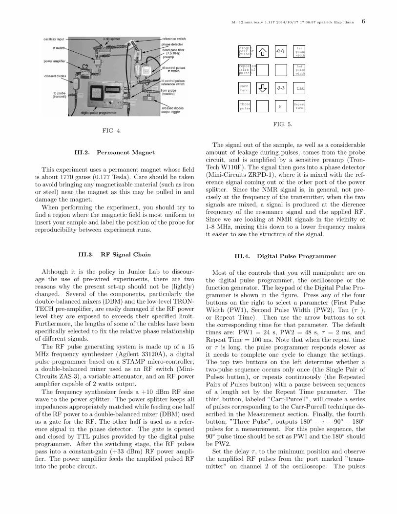
The experimental apparatus, shown schematically in the following figure, consists of a gated RF pulse gen-erator with variable pulse widths and spacings, a probe circuit that delivers RF power to the sample and picks up the signal from the sample, a preamp that amplifies the signal, and a phase detector which outputs an au-dio signal whose frequency corresponds to the difference between the Larmor frequency and the frequency of the signal generator. Details of how to design and build NMR probes can be found in R. Ernst and W. Anderson, Rev. Sci. Instrum. 37, 93 (1966).

6 Id: 12.nmr.tex,v 1.117 2014/10/17 17:36:57 spatrick Exp ldana

CarrPurc.

1st pulsewidth

2nd pulsewidth

tau

RepeatTimeN

singlepair ofpulses

repeatedpairs ofpulses

Threepulse

FIG. 4.

III.2. Permanent Magnet

This experiment uses a permanent magnet whose field is about 1770 gauss (0.177 Tesla). Care should be taken to avoid bringing any magnetizable material (such as iron or steel) near the magnet as this may be pulled in and damage the magnet. When performing the experiment, you should try to

find a region where the magnetic field is most uniform to insert your sample and label the position of the probe for reproducibility between experiment runs.

III.3. RF Signal Chain

Although it is the policy in Junior Lab to discour-age the use of pre-wired experiments, there are two reasons why the present set-up should not be (lightly) changed. Several of the components, particularly the double-balanced mixers (DBM) and the low-level TRON-TECH pre-amplifier, are easily damaged if the RF power level they are exposed to exceeds their specified limit. Furthermore, the lengths of some of the cables have been specifically selected to fix the relative phase relationship of different signals. The RF pulse generating system is made up of a 15

MHz frequency synthesizer (Agilent 33120A), a digital pulse programmer based on a STAMP micro-controller, a double-balanced mixer used as an RF switch (Mini-Circuits ZAS-3), a variable attenuator, and an RF power amplifier capable of 2 watts output. The frequency synthesizer feeds a +10 dBm RF sine

wave to the power splitter. The power splitter keeps all impedances appropriately matched while feeding one half of the RF power to a double-balanced mixer (DBM) used as a gate for the RF. The other half is used as a refer-ence signal in the phase detector. The gate is opened and closed by TTL pulses provided by the digital pulse programmer. After the switching stage, the RF pulses pass into a constant-gain (+33 dBm) RF power ampli-fier. The power amplifier feeds the amplified pulsed RF into the probe circuit.

FIG. 5.

The signal out of the sample, as well as a considerable amount of leakage during pulses, comes from the probe circuit, and is amplified by a sensitive preamp (Tron-Tech W110F). The signal then goes into a phase detector (Mini-Circuits ZRPD-1), where it is mixed with the ref-erence signal coming out of the other port of the power splitter. Since the NMR signal is, in general, not pre-cisely at the frequency of the transmitter, when the two signals are mixed, a signal is produced at the dierence frequency of the resonance signal and the applied RF. Since we are looking at NMR signals in the vicinity of 1-8 MHz, mixing this down to a lower frequency makes it easier to see the structure of the signal.

III.4. Digital Pulse Programmer

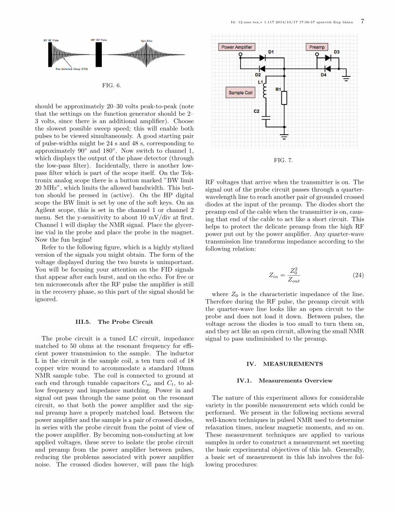
Most of the controls that you will manipulate are on the digital pulse programmer, the oscilloscope or the function generator. The keypad of the Digital Pulse Pro-grammer is shown in the figure. Press any of the four buttons on the right to select a parameter (First Pulse Width (PW1), Second Pulse Width (PW2), Tau (τ ), or Repeat Time). Then use the arrow buttons to set the corresponding time for that parameter. The default times are: PW1 = 24 s, PW2 = 48 s, τ = 2 ms, and Repeat Time = 100 ms. Note that when the repeat time or τ is long, the pulse programmer responds slower as it needs to complete one cycle to change the settings. The top two buttons on the left determine whether a two-pulse sequence occurs only once (the Single Pair of Pulses button), or repeats continuously (the Repeated Pairs of Pulses button) with a pause between sequences of a length set by the Repeat Time parameter. The third button, labeled ”Carr-Purcell”, will create a series of pulses corresponding to the Carr-Purcell technique de-scribed in the Measurement section. Finally, the fourth button, ”Three Pulse”, outputs 180◦ − τ − 90◦ − 180◦

pulses for a measurement. For this pulse sequence, the 90◦ pulse time should be set as PW1 and the 180◦ should be PW2. Set the delay τ , to the minimum position and observe

the amplified RF pulses from the port marked ”trans-mitter” on channel 2 of the oscilloscope. The pulses

7 Id: 12.nmr.tex,v 1.117 2014/10/17 17:36:57 spatrick Exp ldana

FIG. 6.

should be approximately 20–30 volts peak-to-peak (note that the settings on the function generator should be 2– 3 volts, since there is an additional amplifier). Choose the slowest possible sweep speed; this will enable both pulses to be viewed simultaneously. A good starting pair of pulse-widths might be 24 s and 48 s, corresponding to approximately 90◦ and 180◦ . Now switch to channel 1, which displays the output of the phase detector (through the low-pass filter). Incidentally, there is another low-pass filter which is part of the scope itself. On the Tek-tronix analog scope there is a button marked ”BW limit 20 MHz”, which limits the allowed bandwidth. This but-ton should be pressed in (active). On the HP digital scope the BW limit is set by one of the soft keys. On an Agilent scope, this is set in the channel 1 or channel 2 menu. Set the y-sensitivity to about 10 mV/div at first. Channel 1 will display the NMR signal. Place the glycer-ine vial in the probe and place the probe in the magnet. Now the fun begins! Refer to the following figure, which is a highly stylized

version of the signals you might obtain. The form of the voltage displayed during the two bursts is unimportant. You will be focusing your attention on the FID signals that appear after each burst, and on the echo. For five or ten microseconds after the RF pulse the amplifier is still in the recovery phase, so this part of the signal should be ignored.

III.5. The Probe Circuit

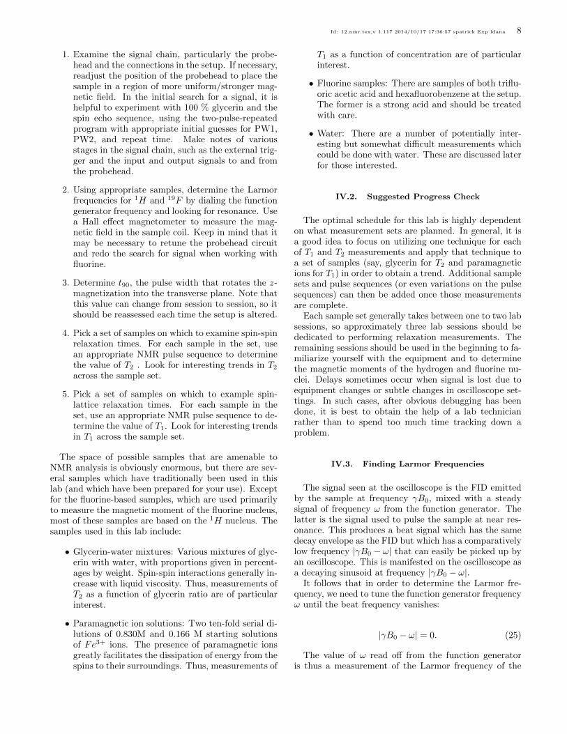
The probe circuit is a tuned LC circuit, impedance matched to 50 ohms at the resonant frequency for effi-cient power transmission to the sample. The inductor L in the circuit is the sample coil, a ten turn coil of 18 copper wire wound to accommodate a standard 10mm NMR sample tube. The coil is connected to ground at each end through tunable capacitors Cm and Ct, to al-low frequency and impedance matching. Power in and signal out pass through the same point on the resonant circuit, so that both the power amplifier and the sig-nal preamp have a properly matched load. Between the power amplifier and the sample is a pair of crossed diodes, in series with the probe circuit from the point of view of the power amplifier. By becoming non-conducting at low applied voltages, these serve to isolate the probe circuit and preamp from the power amplifier between pulses, reducing the problems associated with power amplifier noise. The crossed diodes however, will pass the high

FIG. 7.

RF voltages that arrive when the transmitter is on. The signal out of the probe circuit passes through a quarter-wavelength line to reach another pair of grounded crossed diodes at the input of the preamp. The diodes short the preamp end of the cable when the transmitter is on, caus-ing that end of the cable to act like a short circuit. This helps to protect the delicate preamp from the high RF power put out by the power amplifier. Any quarter-wave transmission line transforms impedance according to the following relation:

Z2 0Zin = (24)

Zout

where Z0 is the characteristic impedance of the line. Therefore during the RF pulse, the preamp circuit with the quarter-wave line looks like an open circuit to the probe and does not load it down. Between pulses, the voltage across the diodes is too small to turn them on, and they act like an open circuit, allowing the small NMR signal to pass undiminished to the preamp.

IV. MEASUREMENTS

IV.1. Measurements Overview

The nature of this experiment allows for considerable variety in the possible measurement sets which could be performed. We present in the following sections several well-known techniques in pulsed NMR used to determine relaxation times, nuclear magnetic moments, and so on. These measurement techniques are applied to various samples in order to construct a measurement set meeting the basic experimental objectives of this lab. Generally, a basic set of measurement in this lab involves the fol-lowing procedures:

8 Id: 12.nmr.tex,v 1.117 2014/10/17 17:36:57 spatrick Exp ldana

1. Examine the signal chain, particularly the probe-head and the connections in the setup. If necessary, readjust the position of the probehead to place the sample in a region of more uniform/stronger mag-netic field. In the initial search for a signal, it is helpful to experiment with 100 % glycerin and the spin echo sequence, using the two-pulse-repeated program with appropriate initial guesses for PW1, PW2, and repeat time. Make notes of various stages in the signal chain, such as the external trig-ger and the input and output signals to and from the probehead.

2. Using appropriate samples, determine the Larmor frequencies for 1H and 19F by dialing the function generator frequency and looking for resonance. Use a Hall effect magnetometer to measure the mag-netic field in the sample coil. Keep in mind that it may be necessary to retune the probehead circuit and redo the search for signal when working with fluorine.

3. Determine t90, the pulse width that rotates the z -magnetization into the transverse plane. Note that this value can change from session to session, so it should be reassessed each time the setup is altered.

4. Pick a set of samples on which to examine spin-spin relaxation times. For each sample in the set, use an appropriate NMR pulse sequence to determine the value of T2 . Look for interesting trends in T2

across the sample set.

5. Pick a set of samples on which to example spin-lattice relaxation times. For each sample in the set, use an appropriate NMR pulse sequence to de-termine the value of T1. Look for interesting trends in T1 across the sample set.

The space of possible samples that are amenable to NMR analysis is obviously enormous, but there are sev-eral samples which have traditionally been used in this lab (and which have been prepared for your use). Except for the fluorine-based samples, which are used primarily to measure the magnetic moment of the fluorine nucleus, most of these samples are based on the 1H nucleus. The samples used in this lab include:

• Glycerin-water mixtures: Various mixtures of glyc-erin with water, with proportions given in percent-ages by weight. Spin-spin interactions generally in-crease with liquid viscosity. Thus, measurements of T2 as a function of glycerin ratio are of particular interest.

• Paramagnetic ion solutions: Two ten-fold serial di-lutions of 0.830M and 0.166 M starting solutions of Fe3+ ions. The presence of paramagnetic ions greatly facilitates the dissipation of energy from the spins to their surroundings. Thus, measurements of

T1 as a function of concentration are of particular interest.

• Fluorine samples: There are samples of both triflu-oric acetic acid and hexafluorobenzene at the setup. The former is a strong acid and should be treated with care.

• Water: There are a number of potentially inter-esting but somewhat difficult measurements which could be done with water. These are discussed later for those interested.

IV.2. Suggested Progress Check

The optimal schedule for this lab is highly dependent on what measurement sets are planned. In general, it is a good idea to focus on utilizing one technique for each of T1 and T2 measurements and apply that technique to a set of samples (say, glycerin for T2 and paramagnetic ions for T1) in order to obtain a trend. Additional sample sets and pulse sequences (or even variations on the pulse sequences) can then be added once those measurements are complete. Each sample set generally takes between one to two lab

sessions, so approximately three lab sessions should be dedicated to performing relaxation measurements. The remaining sessions should be used in the beginning to fa-miliarize yourself with the equipment and to determine the magnetic moments of the hydrogen and fluorine nu-clei. Delays sometimes occur when signal is lost due to equipment changes or subtle changes in oscilloscope set-tings. In such cases, after obvious debugging has been done, it is best to obtain the help of a lab technician rather than to spend too much time tracking down a problem.

IV.3. Finding Larmor Frequencies

The signal seen at the oscilloscope is the FID emitted by the sample at frequency γB0, mixed with a steady signal of frequency ω from the function generator. The latter is the signal used to pulse the sample at near res-onance. This produces a beat signal which has the same decay envelope as the FID but which has a comparatively low frequency |γB0 − ω| that can easily be picked up by an oscilloscope. This is manifested on the oscilloscope as a decaying sinusoid at frequency |γB0 − ω|. It follows that in order to determine the Larmor fre-

quency, we need to tune the function generator frequency ω until the beat frequency vanishes:

|γB0 − ω| = 0. (25)

The value of ω read off from the function generator is thus a measurement of the Larmor frequency of the

9 Id: 12.nmr.tex,v 1.117 2014/10/17 17:36:57 spatrick Exp ldana

sample magnetization. On the scope, the approach to resonance should look like a decaying sinusoid as its fre-quency goes to zero (or its period goes to infinity): the result is simply an exponential decay. Another way to think about this measurement is to

consider the mixing as a ”stroboscopic” view of the mag-netization vector with strobe frequency ω, used to ob-serve the precessing magnetization which has natural fre-quency γB0. When the strobe frequency matches the natural frequency, the magnetization vector appears to stay stationary in the transverse plane, and it simply ap-pears to decay away with the time constant T ∗ .2 Once the Larmor frequency ω = γB0 has been found,

it is necessary also to measure the magnetic field seen by the sample. This is accomplished using a Hall effect mag-netometer, which is shared by several other experiments and so is not a part of the permanent setup. Make cer-tain to zero and calibrate the magnetometer before use and make measurements perpendicular to the magnetic field lines. Estimate the variations in the magnetic field over the sample. Once the resonance frequency has been found, it is

useful to return the oscillator frequency back to being slightly off resonance. Being able to observe a beat signal carried by the exponential decay envelope makes identi-fying and assessing pulse sequences easier. As long as ω ≈ γB0, it is still possible to perform rotations of the magnetization. Adjust ω around resonance to obtain a satisfactory FID signal.

IV.4. Finding Pulse Widths

To obtain an FID signal, it is unnecessary to use the exact value of t90 when pulsing the sample. When first searching for a signal or when making resonance mea-surements to find the Larmor frequency, almost any rea-sonable initial guess for PW1 will result in an observable FID signal (since α 6 0) . However, when utilizing es-= tablished NMR pulse sequences, it is important to have accurate values of t90 and t180 to use. As we mentioned before, it is difficult to know the

magnitude of the perturbing field B1, so the formula t90 = π/γB1 is not very helpful. However, we do know the amplitude of the FID should be maximum after a 90 pulse and minimum or zero after a 180 pulse. Thus, one easy way to obtain the pulse widths is to find the setting of PW1 which minimizes the FID. This gives t180 and halving that gives t90. Another method is to use spin echoes. Set PW1 to

some initial value and set PW2 to be exactly twice PW1. Then adjust PW1 (keeping PW2 twice PW1) until a spin echo is visible and is maximal. Then PW1 gives t90 while PW2 gives t180 . Obviously, there are many other ways in which the pulse widths can be obtained. Experiment with these or other techniques in order to

estimate the 90◦ and 180◦ pulse widths as closely as possi-ble. However, it is important also to realize that the pulse

programmer is only capable of setting PW1 and PW2 in units of 1 s each. Thus, it is only profitable to narrow down the pulse widths to within one or two microsec-onds. Generally, pulse sequences and measurements of relaxation times work well even if the pulse widths are slightly off. When in doubt, it may be helpful to test how big of an effect that changes in PW1 and PW2 make on specific pulse sequences. Note that the values of t90 and t180 are subject to

change from one session to the next, depending on the tuning of the probehead circuit, the power output of the function generator, the exact placement of the sample in the magnetic field, and so on. Thus, it is a good idea to quickly check the pulse widths every session for consis-tency.

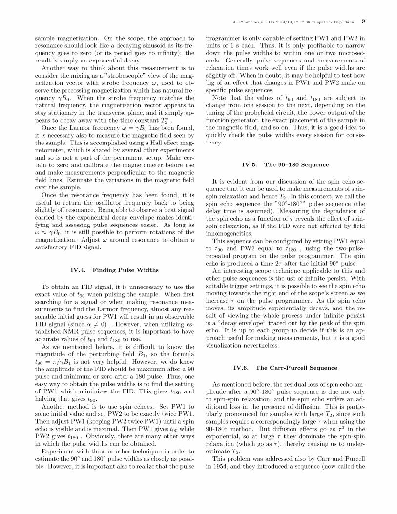
IV.5. The 90–180 Sequence

It is evident from our discussion of the spin echo se-quence that it can be used to make measurements of spin-spin relaxation and hence T2. In this context, we call the spin echo sequence the ”90◦-180◦” pulse sequence (the delay time is assumed). Measuring the degradation of the spin echo as a function of τ reveals the effect of spin-spin relaxation, as if the FID were not affected by field inhomogeneities. This sequence can be configured by setting PW1 equal

to t90 and PW2 equal to t180 , using the two-pulse-repeated program on the pulse programmer. The spin echo is produced a time 2τ after the initial 90◦ pulse. An interesting scope technique applicable to this and

other pulse sequences is the use of infinite persist. With suitable trigger settings, it is possible to see the spin echo moving towards the right end of the scope’s screen as we increase τ on the pulse programmer. As the spin echo moves, its amplitude exponentially decays, and the re-sult of viewing the whole process under infinite persist is a ”decay envelope” traced out by the peak of the spin echo. It is up to each group to decide if this is an ap-proach useful for making measurements, but it is a good visualization nevertheless.

IV.6. The Carr-Purcell Sequence

As mentioned before, the residual loss of spin echo am-plitude after a 90◦-180◦ pulse sequence is due not only to spin-spin relaxation, and the spin echo suffers an ad-ditional loss in the presence of diffusion. This is partic-ularly pronounced for samples with large T2, since such samples require a correspondingly large τ when using the 90-180◦ method. But diffusion effects go as τ3 in the exponential, so at large τ they dominate the spin-spin relaxation (which go as τ ), thereby causing us to under-estimate T2. This problem was addressed also by Carr and Purcell

in 1954, and they introduced a sequence (now called the

Id: 12.nmr.tex,v 1.117 2014/10/17 17:36:57 spatrick Exp ldana 10

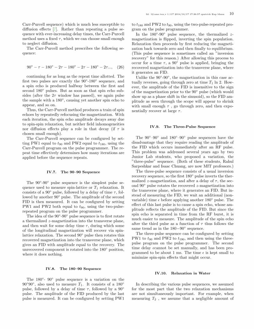
Carr-Purcell sequence) which is much less susceptible to diffusion effects [7]. Rather than repeating a pulse se-quence with ever-increasing delay times, the Carr-Purcell method uses a fixed τ , which we can choose small enough to neglect diffusion. The Carr-Purcell method prescribes the following se-

quence:

90◦ − τ − 180◦ − 2τ − 180◦ − 2τ − 180◦ − 2τ..., (26)

continuing for as long as the repeat time allotted. The first two pulses are exactly the 90◦-180◦ sequence, and a spin echo is produced halfway between the first and second 180◦ pulses. But as soon as that spin echo sub-sides (after the 2τ window has passed), we again pulse the sample with a 180◦, causing yet another spin echo to appear, and so on. Thus, the Carr-Purcell method produces a train of spin

echoes by repeatedly refocusing the magnetization. With each iteration, the spin echo amplitude decays away due to spin-spin relaxation, but neither field inhomogeneities nor diffusion effects play a role in that decay (if τ is chosen small enough). The Carr-Purcell sequence can be configured by set-

ting PW1 equal to t90 and PW2 equal to t180, using the Carr-Purcell program on the pulse programmer. The re-peat time effectively determines how many iterations are applied before the sequence repeats.

IV.7. The 90–90 Sequence

The 90◦-90◦ pulse sequence is the simplest pulse se-quence used to measure spin-lattice or T1 relaxation. It consists of a 90◦ pulse, followed by a delay of time τ , fol-lowed by another 90◦ pulse. The amplitude of the second FID is then measured. It can be configured by setting PW1 and PW2 both equal to t90, using the two-pulse-repeated program on the pulse programmer. The idea of the 90◦-90◦ pulse sequence is to first rotate

a thermalized z -magnetization into the transverse plane, and then wait for some delay time τ , during which some of the longitudinal magnetization will recover via spin-lattice relaxation. The second 90◦ pulse then rotates this recovered magnetization into the transverse plane, which gives an FID with amplitude equal to the recovery. The unrecovered component is rotated into the 180◦ position, where it does nothing.

IV.8. The 180–90 Sequence

The 180◦- 90◦ pulse sequence is a variation on the 90◦90◦, also used to measure T1. It consists of a 180◦

pulse, followed by a delay of time τ , followed by a 90◦

pulse. The amplitude of the FID produced by the last pulse is measured. It can be configured by setting PW1

to t180 and PW2 to t90, using the two-pulse-repeated pro-gram on the pulse programmer. In the 180◦-90◦ pulse sequence, the thermalized z -

magnetization is flipped, inverting the spin population. Relaxation then proceeds by first reducing the magneti-zation back towards zero and then finally to equilibrium. (This pulse sequence is sometimes called an ”inversion recovery” for this reason.) After allowing this process to occur for a time τ , a 90◦ pulse is applied, bringing the recovered magnetization into the transverse plane, where it generates an FID. Unlike the 90◦-90◦, the magnetization in this case ac-

tually reverses, going through zero at time T1 ln 2. How-ever, the amplitude of the FID is insensitive to the sign of the magnetization prior to the 90◦ pulse (which would show up as a phase shift in the sinusoid), so the FID am-plitude as seen through the scope will appear to shrink with small enough τ , go through zero, and then expo-nentially recover at large τ .

IV.9. The Three-Pulse Sequence

The 90◦–90◦ and 180◦–90◦ pulse sequences have the disadvantage that they require reading the amplitude of the FID which occurs immediately after an RF pulse. This problem was addressed several years ago by two Junior Lab students, who proposed a variation, the ”three-pulse” sequence. (Both of these students, Rahul Sarpeshkar and Isaac Chuang, are now MIT professors.) The three-pulse sequence consists of a usual inversion

recovery sequence, so the first 180◦ pulse inverts the ther-malized z -magnetization, and after a delay of τ , the sec-ond 90◦ pulse rotates the recovered z -magnetization into the transverse plane, where it generates an FID. But in-stead of measuring the FID, we wait an additional (non-variable) time � before applying another 180◦ pulse. The effect of this last pulse is to cause a spin echo, whose am-plitude reflects the amplitude of the FID. But since the spin echo is separated in time from the RF burst, it is much easier to measure. The amplitude of the spin echo after the third pulse as a function of τ thus follows the same trend as in the 180−90◦ sequence. The three-pulse sequence can be configured by setting

PW1 to t90 and PW2 to t190, and then using the three-pulse program on the pulse programmer. The second time delay �cannot be set manually, and has been pro-grammed to be about 1 ms. The time � is kept small to minimize spin-spin effects that might occur.

IV.10. Relaxation in Water

In describing the various pulse sequences, we assumed for the most part that the two relaxation mechanisms are not simultaneously important. For example, when measuring T2 , we assume that a negligible amount of

Id: 12.nmr.tex,v 1.117 2014/10/17 17:36:57 spatrick Exp ldana 11

the spin echo decay is due to actual recovery of the z -magnetization via spin-lattice relaxation. For the most part, this assumption is valid when working with samples in which one relaxation constant is drastically smaller than the other (e.g., T2 << T1 in viscous liquids and T1 << T2 in paramagnetic solutions).

Of course, whether this assumption is valid for any particular sample is something which deserves considera-tion in analyzing your results. In fact, this assumption is not quite true for many samples used in NMR, where T1

and T2 are usually comparable. An important example is water, where both of the relaxation constants are on the order of several seconds, making measurements of both quite difficult.

There is, however, at least one interesting way to mea-sure T1 in water which deserves mentioning. As discussed previously, if we want each pulse sequence to yield an in-dependent measurement, we must set the repeat time on the pulse programmer sufficiently large to allow rether-malization. For example, executing two spin echo se-quences too close together will make the second spin echo appear smaller. This suggests that we can actually take advantage of this fact to make a measurement of T1 us-ing spin echoes and by varying not the delay time but the repeat time.

Use the standard spin-echo sequence (90◦–180◦) with some fixed time constant τ . Record the spin echo height produced when repeating the sequence using a variable repeat time; the spin echo height as a function of the repeat time should give the exponential return of the magnetization with time constant T1. For higher repeat times higher than 3 s, you can use the two-pulse-single program on the pulse programmer and a watch, rather than the two-pulse-repeated program. As an optional experiment, perform these measurements with both tap water and distilled water. Is it possible to detect the difference?

The first measurements of T1 in distilled water stood for about thirty years. Since then, careful measurements have produced a number which is about 50% higher. The difference is due to the effect of dissolved oxygen in the water, as O2 is paramagnetic. As an optional experiment, try to remove the dissolved oxygen from a sample of dis-tilled water and see if there is any difference. One way this could be done is by bubbling pure nitrogen through

the water, as N2 is diamagnetic.

V. ANALYSIS

Due to the wide range of possible measurements in this experiment, there is a corresponding variety in the particular analysis approach that best suits your data set. However, some results that are often presented include the following:

• The Larmor frequencies and gyromagnetic ratios of the proton and 19F nucleus.

• Demonstration of the successful use of a pulse se-quence to measure the spin-lattice relaxation time T1 across a range of samples (e.g., paramagnetic ion solutions).

• Demonstration of the successful use of a pulse se-quence to measure the spin-lattice relaxation time T2 across a range of samples (e.g., paramagnetic ion solutions).

The idea is to structure the measurement sets and anal-ysis so that you can make a case for the effectiveness of NMR as a way of probing the microscopic structure of your samples, by demonstrating measurements that are sensitive to changes in the material structure. You may find throughout the experiment that some samples are easier to work with than others. Time constraints can also dictate which measurement sets to use and what analysis approach to take. One interesting idea often pursued is to reproduce the

early results by Bloembergen and Purcell when working with water-glycerin mixtures, such as those in [2] and Bloembergen’s thesis [8]. They found that plotting the relaxation constants against logarithm of viscosity (or concentration) resulted in interesting curves as the vis-cocity (concentration) varied over a large range. Tables relating percent weight of glycerin to viscosity can be found in tables like this one collected by DOW. Remember as always to address sources of errors or

uncertainty in your results, quantitatively whenever pos-sible. Each pulse sequence is susceptible to different sources of systematic effects (e.g., diffusion in the 90◦180◦

sequence), so interpretation of the results needs to take into account an understanding of the physics behind the technique. In some ways, this one of the central ideas behind NMR spectroscopy.

[1] F. Bloch, Phys. Rev. 70, 460 (1946). [5] A. Abragam, Principles of Nuclear Magnetism (Ox-[2] N. Bloembergen, E. Purcell, and R. Pound, Phys. Rev. ford University Press, 1961) physics Department Reading

73, 679 (1948). Room. [3] F. Bloch, Nobel Lecture (1952). [6] M. Levitt, Spin Dynamics: Basics of Nuclear Magnetic [4] E. M. Purcell, Nobel Lecture (1952). Resonance.

[7] H. Carr and E. Purcell, Phys. Rev. 94, 630 (1954).

Id: 12.nmr.tex,v 1.117 2014/10/17 17:36:57 spatrick Exp ldana 12

[8] N. Bloembergen, Nuclear Magnetic Relaxation (W.A. Benjamin, 1961) physics Department Reading Room.

Appendix A: Quantum Mechanical Description of NMR

Recall that for all spin-1/2 particles (protons, neu-trons, electrons, quarks, leptons), there are just two

1eigenstates: spin up |S, Sz i = | 1 , i ≡ |0i and spin down 2 2 |S, Szi = | 1 , − 1 i ≡ |1i. Using these as basis vectors, the 2 2 general state of a spin-1/2 particle can be expressed as a two-element column matrix called a spinor : � �

u|ψi = u|0i + d|1i = . (A1)d

Normalization imposes the constraint |u|2 + |d|2 = 1. The system is governed by the Schrodinger equation

d i~ |ψi = H|ψi, (A2)dt

which has the solution |ψ(t)i = U |ψ(0)i, where U = −iHt/~ e is unitary. In pulsed NMR, the Hamiltonian

~H = −~µ · B = −µ [σxBx + σyBy + σzBz ] (A3)

is the potential energy of a magnetic moment placed in an external magnetic field. The σi are the Pauli spin matrices: � �

0 1 σx ≡ ,

1 0 � � 0 −i

σy ≡ ,i 0 � � 1 0

σz ≡ . (A4)0 −1

Inserting Equations (A4), (A1), and (A3) into Equa-tion (A2), we get

u = (µ/~) [iBx + By ] d + i(µ/~)Bz u,

d = (µ/~) [iBx − By ] u − i(µ/~)Bzd. (A5)

If Bx = By = 0 and the equations reduce to

u = i(µ/~)Bzu,

d = −i(µ/~)Bz d. (A6)

Integrating with respect to time yields

i(µ/~)Bz t iω0t/2 u =u0e = u0e , −i(µ/~)Bz t −iω0t/2d =d0e = d0e , (A7)

where ω0 = 2µBz/~ is the Larmor precession frequency. If an atom undergoes a spin-flip transition from the spin up state to the spin down state, the emitted photon has energy E = ω0 ~.

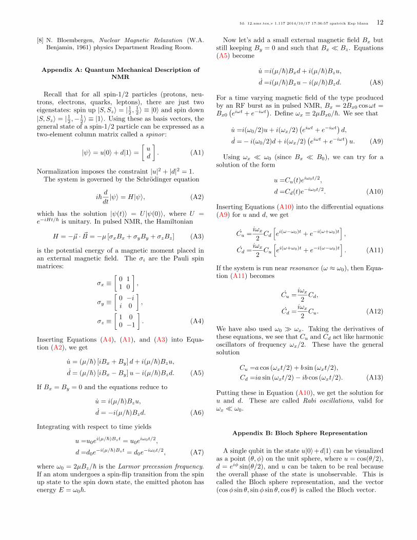
Now let’s add a small external magnetic field Bx but still keeping By = 0 and such that Bx � Bz. Equations (A5) become

u =i(µ/~)Bxd + i(µ/~)Bzu,

d =i(µ/~)Bxu − i(µ/~)Bzd. (A8)

For a time varying magnetic field of the type produced by an RF burst as in pulsed NMR, Bx = 2Bx0 cos ωt = � �

iωt −iωt Bx0 e + e . Define ωx ≡ 2µBx0/~. We see that � �iωt −iωtu =i(ω0/2)u + i(ωx/2) e + e d, � �

iωt −iωtd = − i(ω0/2)d + i(ωx/2) e + e u. (A9)

Using ωx � ω0 (since Bx � B0), we can try for a solution of the form

iω0t/2 u =Cu(t)e , −iω0t/2d =Cd(t)e . (A10)

Inserting Equations (A10) into the differential equations (A9) for u and d, we get h iiωx i(ω−ω0)t −i(ω+ω0)tC

u = Cd e + e ,2 h iiωx i(ω+ω0)t −i(ω−ω0)tCd = Cu e + e . (A11)2

If the system is run near resonance (ω ≈ ω0), then Equa-tion (A11) becomes

iωxC

u = Cd,2 iωx

C d = Cu. (A12)

2

We have also used ω0 � ωx. Taking the derivatives of these equations, we see that Cu and Cd act like harmonic oscillators of frequency ωx/2. These have the general solution

Cu =a cos (ωxt/2) + b sin (ωxt/2),

Cd =ia sin (ωxt/2) − ib cos (ωxt/2). (A13)

Putting these in Equation (A10), we get the solution for u and d. These are called Rabi oscillations, valid for ωx � ω0.

Appendix B: Bloch Sphere Representation

A single qubit in the state u|0i+ d|1i can be visualized as a point (θ, φ) on the unit sphere, where u = cos(θ/2), d = eiφ sin(θ/2), and u can be taken to be real because the overall phase of the state is unobservable. This is called the Bloch sphere representation, and the vector (cos φ sin θ, sin φ sin θ, cos θ) is called the Bloch vector.

Id: 12.nmr.tex,v 1.117 2014/10/17 17:36:57 spatrick Exp ldana 13

The Pauli matrices give rise to three useful classes of unitary matrices when they are exponentiated, the rota-tion operators about the x, y, and z axes, defined by the equations:

θ θ−iθσx/2Rx(θ) ≡e = cos I − i sin σx2 2� �

θ cos −i sin θ 2 2= , (B1)θ−i sin θ cos2 2

θ θ−iθσy /2Ry(θ) ≡e = cos I − i sin σy2 2� �

θ cos − sin θ 2 2= , (B2)

sin θ 2 cos θ

2

θ θ−iθσz /2Rz (θ) ≡e = cos I − i sin σz2 2� � −iθ/2e 0

= . (B3)iθ/20 e

One reason why the Rn(θ) operators are referred to as rotation operators is the following fact. Suppose a single qubit has a state represented by the Bloch vector ~λ. Then the effect of the rotation Rn(θ) on the state is to rotate it by an angle θ about the n axis of the Bloch sphere. An arbitrary unitary operator on a single qubit can

be written in many ways as a combination of rotations, together with global phase shifts on the qubit. A useful theorem to remember is the following: Suppose U is a unitary operation on a single qubit. Then there exist real numbers α, β, γ and δ such that

iαRxU = e (β)Ry (γ)Rx(δ). (B4)

Appendix C: Fundamental equations of magnetic resonance

The magnetic interaction of a classical electromagnetic field with a two-state spin is described by the Hamil-

~tonian H = −~µ · B, where µ~ is the spin, and B = B0z+B1(x cos ωt+ y sin ωt) is a typical applied magnetic field. B0 is static and very large, and B1 is usually time varying and several orders of magnitude smaller than B0

in strength, so that perturbation theory is traditionally employed to study this system. However, the Schrodinger equation for this system can be solved straightforwardly without perturbation theory. The Hamiltonian can be written as

~ω0H = Z + ~g(X cos ωt + Y sin ωt), (C1)

2

where g is related to the strength of the B1 field, and ω0

to B0, and X, Y , and Z are introduced as a shorthand for the Pauli matrices. Define |φ(t)i = eiωtZ/2|χ(t)i, such that the Schrodinger equation

i~∂t|χ(t)i = H|χ(t)i (C2)

can be re-expressed as � � ~ωiωZt/2He−iωZt/2 −i~∂t|φ(t)i = e Z |φ(t)i. (C3)2

Since

iωZt/2Xe−iωZt/2 = (X cos ωt − Y sin ωt),e (C4)

Equation (C3) simplifies to become � � ω0 − ω

i∂t|φ(t)i = Z + gX |φ(t)i, (C5)2

where the terms on the right multiplying the state can be identified as the effective “rotating frame” Hamiltonian. The solution to this equation is � �

ω0 −ωi Z+gX t

|φ(t)i = e 2 |φ(0)i. (C6)

The concept of resonance arises from the behavior of this solution, which can be understood to be a single qubit rotation about the axis

2gz + xω0 −ω n = r (C7)� �2 2g1 + ω0−ω

by an angle s� �2ω0 − ω |~n| = t + g2 . (C8)2

When ω is far from ω0, the spin is negligibly affected by the B1 field; the axis of its rotation is nearly parallel with z, and its time evolution is nearly exactly that of the free B0 Hamiltonian. On the other hand, when ω0 ≈ ω, the B0 contribution becomes negligible, and a small B1

field can cause large changes in the state, corresponding to rotations about the x axis. The enormous effect a small perturbation can have on the spin system, when tuned to the appropriate frequency, is responsible for the ‘resonance’ in nuclear magnetic resonance. In general, when ω = ω0, the single spin rotating frame

Hamiltonian can be written as

H = g1(t)X + g2(t)Y, (C9)

where g1 and g2 are functions of the applied transverse RF fields.

Appendix D: Modeling the NMR Probe

The material in this appendix was provided by Profes-sor Isaac Chuang. A tuned circuit is typically used to efficiently irradiate a sample with electromagnetic fields in the radiofrequency of microwave regime. This circuit allows power to be transferred from a source with min-imal reflection, while at the same time creating a large electric of magnetic field around the sample, which is typically placed within a coil that is part of it.

Id: 12.nmr.tex,v 1.117 2014/10/17 17:36:57 spatrick Exp ldana 14

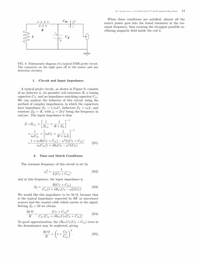
When these conditions are satisfied, almost all the source power goes into the tuned resonator at the res-onant frequency, thus creating the strongest possible os-cillating magnetic field inside the coil L.

FIG. 8. Schematatic diagram of a typical NMR probe circuit. The connector on the right goes off to the source and any detection circuitry.

1. Circuit and Input Impedance

A typical probe circuit, as shown in Figure 9, consists of an inductor L, its parasitic coil resistance R, a tuning capacitor CT , and an impedance matching capacitor Cm. We can analyze the behavior of this circuit using the method of complex impedances, in which the capacitors have impedance ZC = 1/iωC, inductors ZL = iωL, and resistors ZR = R, with ω = 2πf being the frequency in rad/sec. The input impedance is thus �

1 1 �−1

Z =ZCm + ZCT

+ R + ZL

1 �

1 �−1

= + iωCT + iωCm R + iωL

1 + iωR(CT + Cm) − ω2L(CT + Cm) = . (D1)

iωCm(1 + iRωCT − ω2LCT )

2. Tune and Match Conditions

The resonant frequency of this circuit is set by

1 ω2 = , (D2)∗ L(CT + Cm)

and at this frequency, the input impedance is

R(CT + Cm)Z0 = . (D3)

Cm(1 + iRω∗CT − ω∗2LCT )

We would like this impedance to be 50 Ω, because that is the typical impedance expected by RF or microwave sources and the coaxial cable which carries in the signal. Setting Z0 = 50 we obtain:

50 Ω (CT + Cm)2

= . (D4)R Cm [Cm + iRω∗CT (CT + Cm)]

To good approximation, the iRω∗CT (CT + Cm) term in the denominator may be neglected, giving � �2

50 Ω CT = 1 + . (D5)

R Cm

MIT OpenCourseWare https://ocw.mit.edu

8.13-14 Experimental Physics I & II "Junior Lab" Fall 2016 - Spring 2017

For information about citing these materials or our Terms of Use, visit: https://ocw.mit.edu/terms.