Inference from multiple imputation for missing data usingmixtures of normalsRussell J. Steele a, Naisyin Wang b, Adrian E. Raftery c,∗aMcGill University, Canadab University of Michigan, USAc University of Washington, USA
a r t i c l e i n f o
Article history:Received 25 April 2009Received in revised form8 January 2010Accepted 8 January 2010
Keywords:Importance samplingImproper imputationQuality of life
a b s t r a c t
We consider two difficulties with standard multiple imputationmethods formissing data based on Rubin’s tmethod for confidenceintervals: their often excessive width, and their instability. Theseproblems are present most often when the number of copies issmall, as is often the case when a data-collection organizationis making multiple completed datasets available for analysis. Wesuggest using mixtures of normals as an alternative to Rubin’st . We also examine the performance of improper imputationmethods as an alternative to generating copies from the trueposterior distribution for the missing observations. We report theresults of simulation studies and analyses of data on health-relatedquality of life in which the methods suggested here gave narrowerconfidence intervals and more stable inferences, especially withsmall numbers of copies or non-normal posterior distributions ofparameter estimates. A free R software package called MImix thatimplements our methods is available from CRAN.
In public health and social research, it is now common for researchers to collect a large amountof information on a big set of subjects. Organizations that collect and provide data often serve usersthat vary in their levels of statistical sophistication. As is standard in the imputation literature, wewillassume here that the data-collection organization has control over the datasets provided to users, but
∗ Corresponding address: Department of Statistics, University of Washington, Box 354322, Seattle, WA 98195-4322, UnitedStates. Tel.: +1 206 543 4505.E-mail address: [email protected] (A.E. Raftery).
not over the analyses they perform. The goal of the data-collection organization is to provide a set ofdata that users can analyze using standard complete data techniques.Usually, the possible recourses for peoplewhowish to analyze such data are to ignore observations
with missing data (row elimination or complete case analysis), to ignore entire variables for whichthere are missing values (column elimination), or to use a more sophisticated statistical technique tohandle the missingness in the data.None of these recourses is very attractive. The first two, which involve ignoring data that were
collected, are inefficient and can lead to biases if the missing data are not missing completely atrandom. For longitudinal clinical studies, they might actually cause one to eliminate a significantfraction of the data collected. The third is the most desirable from a statistical point of view, butrequires a level of technical sophistication beyond that of many users of large databases.Multiple imputation, introduced by Rubin for survey researchers [18,19] and popularized by
Schafer [21] and the accompanying software, is intuitively appealing and relatively straightforward,and is now widely used.The standard approach to inference about individual parameters frommultiple imputation is to use
a confidence interval based on the t distribution. We will show when the number of copies is small,this can lead to confidence intervals that are very wide, unstable, or both. Here we take a differentapproach, approximating the marginal posterior distribution of parameters or quantities of interestby amixture of normals, as has long been a standard approach to density estimation [6,28,4,17,7]. Weshow that this gives narrower confidence intervals and better overall performance than the t-basedintervals.A free R software package called MImix that implements our methods is available at http://cran.r-
project.org.In Section 2 we describe our method, in Section 3 we analyze a simple simulated example, and in
Section 4 we apply our method to a real data set from health-related quality of life research.
2. Methods
We denote the observed data by Y and the missing data by Z , and we assume that the analystis interested in estimating a particular vector-valued estimand of interest (Q ) (e.g. means, medians,regression coefficients, etc.).Rubin [20] addresses the topic from a Bayesian perspective, which we summarize here. A Bayesian
approach to inference about Q centers on the posterior distribution of Q given the observed dataY . One can write the posterior distribution of Q as P(Q |Y , X) =
∫P(Q |Y , Z, X)P(Z |Y , X)dZ , where
P(Z |Y , X) is the posterior distribution of the missing data Z given the observed data and X representsother information that the imputermay have. Note that the imputer is not necessarily the analyst, andmay, for example, be an agency providing a small number of multiply imputed copies of the datasetfor use by others. If one specifies a full probabilitymodel for themissing data, then one can in principlemake posterior inference about Q . The posterior mean and variance of Q are as follows:
E(Q |Y , X) = EZ (EQ (Q |Y , Z, X)|Y , X) (1)
Var(Q |Y , X) = EZ (VarQ (Q |Y , Z, X)|Y , X)+ VarZ (EQ (Q |Y , Z, X)|Y , X)= U + B. (2)
These could be estimated by simulating independent draws from the posterior distribution of themissing data Z , and replacing the expectations over Z in (1) and (2) by sample averages over thesimulated values of Z .Under the multiple imputation paradigm of [18], the imputer generates copies of the missing data
from P(Z |Y , X), a probability model that attempts to model the missing data based on the observedresponses (Y ) and other information for both complete and incomplete cases (X). Conditionally on theprobability model, the following are consistent estimators of Q , U and B:
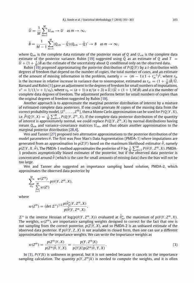
where Q∗m is the complete data estimate of the posterior mean of Q and U∗m is the complete dataestimate of the posterior variance. Rubin [19] suggested using Q as an estimate of Q and T =U + (1+ 1
M )B as the estimate of the uncertainty about Q conditional only on the observed data.Rubin [19] proposed approximating the posterior distribution of P(Q |Y ) by a t-distribution with
degrees of freedom that depend on the number of copies, the total number of cases, and an estimateof the amount of missing information in the problem, namely ν = (m − 1)(1 + r−1m )
2, where rmis the increase in relative increase in variance due to nonresponse, estimated as rm = (1 + 1
M )B/U .Barnard andRubin [1] gave an adjustment to the degrees of freedom for small numbers of imputations,ν∗ = 1/(1/ν + 1/ν0), where ν0 = (a+ 1) ∗ a/(a+ 3) ∗ U/(U + (1+ 1/M)B) and a is the number ofcomplete data degrees of freedom. The adjustment performs better for small numbers of copies thanthe original degrees of freedom suggested by Rubin [19].Another approach is to approximate the marginal posterior distribution of interest by a mixture
of estimated complete data posteriors. If one could generate M copies of the missing data from thecorrect probabilitymodel, {Z1, . . . , ZM}, then aMonte Carlo approximation can be used for P(Q |Y , X),i.e. P(Q |Y , X) = 1
M
∑Mm=1 P(Q |Y , Z
m, X). If the complete data posterior distribution of the quantityof interest is approximately normal, we could replace P(Q |Y , Zm, X) by normal distributions havingmeans Q∗m and variance–covariance matrices U∗m, and thus obtain another approximation to themarginal posterior distribution [28,4].Wei and Tanner [27] proposed two alternative approximations to the posterior distribution of the
model parameters θ . The first was Poor Man’s Data Augmentation (PMDA-1) where imputations aregenerated from an approximation to p(Z |Y ) based on the maximum likelihood estimator θ , namelyp(Z |Y , X, θ ). The PMDA-1method approximates the posterior of θ by 1M
∑Mm=1 P(θ |Y , Z
m, X). PMDA-1 produces asymptotically biased estimates of the posterior, but if the observed data posterior isconcentrated around θ (which is the case for small amounts of missing data) then the bias will not betoo large.Wei and Tanner also suggested an importance sampling based solution, PMDA-2, which
approximates the observed data posterior by
M∑m1
w(Zm)M∑i=1w(Z i)
p(θ |Y , Zm, X),
where
w(Zm) = (detΣ∗)1/2p(θ∗m|Y , Z
m, X)
p(θ |Y , Zm, X),
Σ∗ is the inverse Hessian of log(p(θ |Y , Zm, X)) evaluated at θ∗m, the maximum of p(θ |Y , Zm, X).
The weights, w(Zm), are importance sampling weights designed to correct for the fact that one isnot sampling from the correct posterior, p(Z |Y , X), and so PMDA-2 is an unbiased estimate of theobserved data posterior. If p(θ |Y , Z, X) is not available in closed form, then one can use a differentapproximation for the importance weights. We can write the importance weights as
w(Zm) =p(Zm|Y , X)
p(Zm|θ , Y , X)=
p(Y , Zm|X)
p(Y |X)p(Zm|θ , Y , X). (3)
In (3), P(Y |X) is unknown in general, but it is not needed because it cancels in the importancesampling calculation. The quantity p(Y , Zm|X) is needed to compute the weights, and it is often
not available in closed form. This is the complete data log-integrated likelihood, which can oftenbe approximated by the Schwarz approximation P(Y , Z |X, θm)n−d/2, where d is the number ofparameters and n is the total sample size for the complete data model [23,10].Summarizing via mixtures of normals rather than using a t distribution only slightly increases
the computational burden on the user. In order to obtain point estimates (via the median of theposterior density estimate) and 95% confidence (or credible) limits, the user must simply obtain therequired percentiles of the mixture distribution. Obtaining the desired mixture percentile values (saycj) requires solving
M∑m=1
w(zm)φ(q, θm, σ (θm)) = cj
for q where φ represents the normal density. Numerical root-finding methods (typically availablein statistical software) can be used to solve for q. If the user does not have access to such software,they could also generate samples of q from the mixture density and use the Monte Carlo samples toestimate the percentiles of interest.
3. Simulated data example
In this paper, we compare several multiple imputation methods for estimation of functionals ofinterest, focusing on the results for small numbers of copies. It has been shown elsewhere [19,14]that generating copies from the correct posterior distribution is preferable to generating copies froman approximation to the correct posterior as the number of copies used in the estimation tendsto infinity. We will focus on both very small numbers of copies (3 or 5) which makes sense forimputation for ‘‘typical’’ users (and is commonly recommended in texts and software documentationfor computational procedures), and we will also look at performance for 10 and 25 copies, which isfeasible when the storage capacity allows or the research problem demands higher precision. Wewillcompare four methods, two of which are proper, completing the missing observations via their trueposterior distribution, namely Rubin’s t and Monte Carlo methods. One method follows the conceptof PMDA-2, which uses an improper method of imputation generation but still yields asymptoticallycorrect inference for the parameters of interest. The last method is PMDA-1, which is both improperand inconsistent.The simple normal example has proved enlightening in other work [16], and we use it here
as a starting example. Assume that we observe N subjects and wish to estimate a tail probability,i.e. θ = Pr(X < ξ), where we assume that X is normally distributed with an unknown mean µ andvariance σ 2. If none of the N observations is missing, then one can obtain a model-based estimate ofthe tail probability, θ , namely θN = Φ(
ξ−xNsN), where Φ is the cumulative distribution function of the
standard normal.Using the asymptotic normality of θN to make inference about θ via the Delta method, we obtain
θN∼φ(Φ(
ξ−µ
σ), τ (µ, σ , ξ)
)where φ(a, b) indicates the normal density with mean a and variance b.
Here ∼, denotes approximately distributed and
τ(µ, σ , ξ) =
{∂∂µΦ(
ξ−µ
σ)}2σ 2 +
{∂
∂σ 2Φ(
ξ−µ
σ)}22σ 4
Nis the resulting variance from the Delta method. Given a sample x1, . . . , xN , we can estimate µ byxN and σ by sN and use the plug-in approach to obtain an approximate confidence set for the tailprobability of interest.One can also approach the problem as one of estimating the posterior distribution of θ , i.e.
p(θ |x1, . . . , xN). The posterior distribution for θ is not available in closed form, even whenusing the standard Normal-Inverse-χ2 conjugate priors for µ and σ 2. However, we can easilysample from the posterior distribution of µ and σ 2 in closed form, so we could generate anapproximate sample from p(θ |x1, . . . , xN) by first sampling µ and σ 2 from their joint posteriordistribution, and then calculate the resulting θ for each pair. Another possibility is to use a normal
approximation to the posterior via the same delta method approximation used in the frequentistcase, i.e. p(θ |x1, . . . , xN)∼φ(Φ(
ξ−xNsN), τ (xN , sN , ξ)). One can justify this approximation under the
assumption that any reasonably non-informative prior distribution will have negligible effect on thenormality of the likelihood asymptotically [2].In order to evaluate the imputation methods, we now assume that k of the N observations are
missing, leaving N − k = n observed data points. Because the data are missing completely at random(MCAR), the obvious correct inference for the problem is based on the estimator and variance estimateusing only the observed data points, i.e. θn is approximately normal with meanΦ(
ξ−xnsn) and variance
τ(xn, sn, ξ) where xn and s2n are the sample mean and variance of the reduced dataset. However,treating this as amissing data problem allows us to ‘‘impute’’ themissing data and use the ‘‘completeddata’’ x1, . . . , xN to make inference about the parameter of interest for a situation where we knowwhat the correct inference is.We generate M copies of the missing data points x(m)n+1, . . . , x
(m)N according to their true posterior
distribution p(·|x1, . . . , xn), or M copies of x∗(m)n+1 , . . . , x
∗(m)N according to their posterior distribution
conditional on the maximum likelihood estimates, p(·|x1, . . . , xn, µ, σ ). We then calculate xmN andsmN (m = 1, . . . ,M) (or x
∗mN and s∗mN ) for each completed dataset. In each case, the complete data
estimate of the posterior functional of interest is Φ( ξ−xmN
smN) (or Φ( ξ−x
∗mN
s∗mN)). We consider the following
approximations for p(θ |x1, . . . , xn):
• Rubin’s t: a t distribution with mean 1M
∑Mm=1Φ(
ξ−xmNsmN) and variance and degrees of freedom
estimated according to Rubin [19] and Barnard and Rubin [1].• Monte Carlo: a mixture of normal distributions, 1M
∑Mm=1 φ(Φ(
ξ−xmNsmN), τ (xmN , s
mN , ξ))
• PMDA-1: a mixture of normal distributions, 1M∑Mm=1 φ(Φ(
ξ−x∗mNs∗mN
), τ (x∗mN , s∗mN , ξ))
• PMDA-2: an importance weighted mixture of normal distributions,M∑m=1
w(x∗mn+1, . . . , x∗mN )φ
(Φ
(ξ − x∗mNs∗mN
), τ (x∗mN , s
∗mN , ξ)
).
There are at least two advantages toworkingwith our simple example above. First, we can simulatefrom the true posterior distribution of the missing data (no MCMC approximation is necessary). It isin fact the posterior predictive distribution based on the n completely observed data points. Second,we can generate datasets for which we know that the distributional assumptions hold. Therefore anydifferences between the methods must be due to their actual properties as estimators and simpleMonte Carlo variability due to the generation of datasets and the Monte Carlo sampling required ofthe methods, rather than to an incorrect data model or difficulties with generating samples from theposterior distribution.We simulated 10,000 datasets with 150 observations and 20% missingness. We let ξ = − 1.96.
In order to reduce Monte Carlo variability as much as possible, missing observations were generatedusing the same uniform random variables across the four methods and the inverse-CDF transformmethod. Also, an imputed data set with a smaller number of copies was always taken from a subsetof the corresponding imputed set with a largerm.We can evaluate our method from two perspectives. First, we can treat the imputation procedures
as Bayesian approximations to frequentist confidence sets. In that case, we are interested in thefrequentist coverage properties of our estimator and interval, i.e. whether the constructed intervalscontain the true value of θ over repeated datasets with the correct relative frequency. Of course,coverage is not the only concern.We also evaluate the average length of the interval and its variability.In general, we want to reach the correct coverage probability with the shortest interval possible.The second perspective from which we can evaluate our proposed imputation methods is as
an approximation to the true Bayesian posterior interval. We will focus on the Bayesian posteriorcoverage of our intervals, i.e. the amount of the true posterior distribution covered by our intervalresulting from the imputationprocedures. Again,wemust take into account the length of our intervals,
in that we want to have the shortest interval possible that completely covers the true Bayesianposterior interval.From a frequentist perspective, we focus on the performance of one application of our procedure
to a number of simulated datasets. We generated 10,000 datasets from a normal distribution withmean zero and variance 1. For each dataset, we applied each of the imputation methods listed aboveand calculated the length and coverage of the resulting 95% confidence intervals. Fig. 1 shows theestimated coverage probabilities for each of the four methods considered.The coverage probabilities for all 95% confidence intervals lie between 91% and 94%. ForM = 3 and
M = 5 copies, Rubin’s t-method has the best coverage of 92.5%, which is 1% or 1.5% higher than othercases. However, the cost of that coverage is a longer interval. The top-right plot in Fig. 1 shows therelative length of the credible/confidence intervals for the various methods. With 20% missing data,Rubin’smethod yields intervals that are over 10% longer than the standardMonte Carlo intervalswhenm = 3.Frequentist coverage of the true value is not the only consideration, at least from a Bayesian
viewpoint. We also consider the coverage of the true underlying posterior density of the tailprobability of interest. If we view all four imputation methods as attempts to approximate the trueunderlying posterior density of the population tail probability, then we can examine the amount ofposterior probability allocated to the true Bayesian 95% credible interval.The bottom-left plot in Fig. 1 shows the posterior coverages, which range from 92%–95%, for
the four imputation methods. The posterior coverage of Rubin’s method levels off more quickly,which is not surprising as themixture-based estimationmethods are more directly trying to estimatethe features of the underlying posterior distribution, allowing for greater posterior coverage by theapproximations via a mixture of normals. The variability of the posterior coverage of Rubin’s methodis greater, as illustrated by the bottom-right plot of Fig. 1, despite the fact that its average coverage isslightly larger. When considered closely, this is likely the case because, for small numbers of copies,the three imputation statistics of interest, (Q , U , B), will not be particularly robust to ‘‘extreme’’ copiesof the missing data. The posterior density estimate is only one t distribution based on those threeimputation statistics, so any large fluctuation in the summaries could cause a large fluctuation in thet approximation. The mixture approach has the advantage that such ‘‘extreme’’ copies will receiveweight of only 1/M in the density approximation.As pointed out by a reviewer, to refine the inference procedure, one could first construct a
confidence interval for the logit transformed θ and then inversely transform the endpoints. Theadvantage of such an approach is that the asymptotic normality emerges faster in the transformedscenario than in the untransformed one. We did this and obtained equivalent outcomes to that ofconducting direct inferences with θ . With the improved asymptotic normality in the transformedscenario, the coverage probabilities for all procedures improved by about 2%–3%. For M = 3, 5, and10 copies, the improved coverage probabilities for Monte Carlo and the two mixture approaches nowvary between 93%–94% while the coverage probabilities for Rubin’s t now reach 96%. The patternsin the relative lengths of intervals are similar to those given in Fig. 1: the two mixture approachescontinue to give the shortest intervals, while the relative average lengths of Rubin’s method to thoseof the standard Monte Carlo intervals increase slightly from 15%, 6% and 3% forM = 3%, 5%, and 10%to 17%, 8% and 6%, respectively.
4. Example: Missing data in health-related quality of life research
4.1. The model
In this section, we present a more complicated missing data example. Factor analysis models havebeen widely used by researchers in the social and health sciences for complex relationships betweenobserved measurements via latent constructs. In the usual factor analysis setting, one observes a p-dimensional vector of responses, yi = (yi1, . . . , yip) for each of n observations (i = 1., . . . n).The factor analysis model is
Fig. 1. Simulation results for estimation of the lower tail probability, Φ(ξ = −1.96), of a normal distribution for simulatednormal datasets with 20% missing where results are the average over 10,000 random datasets. The top-left figure containsthe estimated frequentist coverage probabilities of the associated 95% intervals. The top-right figure contains average intervallengths relative to the 95% confidence interval length for the mixture method with draws from the true posterior distribution(MC). The lower-left figure contains estimated posterior coverage probabilities for 95% confidence intervals for the lower 2.5thpercentile,Φ(ξ = −1.96). The lower-right figure contains the standard deviation for observed interval lengths relative to the95% confidence interval length for the mixture method with draws from the true posterior distribution (MC).
where µ is a (p × 1) mean vector, Λ is a (p × q) matrix of factor loadings, ωi is a (q × 1) vector oflatent construct measures, and εi is a vector of multivariate normal errors. The vector ωi is typicallyassumed to bemultivariate normal with variance–covariancematrix R; for simplicity, wewill assumethat R = Iq×q. The model errors, εi, represent variability unexplained by the latent factor structureand are assumed to be multivariate normal with diagonal variance–covariance matrix D, wherediag(D) = (σ 21 , . . . , σ
2p ). One can assess the relative ‘‘uniqueness’’ of the variables through the σ
2j
parameters, i.e. the larger the value of σ 2j parameter, the less that variable is explained by the factormodel.Several practical issues arise when utilizing factor analysis for either exploratory or confirmatory
analyses, particularly when using Bayesian methods. First, the factor loadings,Λ, typically have to beconstrained in some way in order for the loadings to be identifiable. We follow Lopes and West [13]and use the approach of Geweke and Zhou [8] to guarantee identifiability of the factor loadings byrestricting Λkk > 0 and Λjk = 0 for j < k. Our restrictions in this context are slightly artificial, butwe use them in order to ensure that the copies from a fully Bayesian analysis are compatible with thecomplete data factor analysis procedure.Even with this restriction it is difficult to make inference for the factor loadings,Λjk. For example,
although one can use asymptotic estimates via numerical differentiation to obtain standard errorestimates for the model parameters, the calculation can be difficult and numerically unstable.Resampling approaches such as the jackknife and bootstrap are often used in place of difficultnumerical methods. We also use the bootstrap approach here to obtain the estimated standard errorsfor the factor loadings. Although the loadings are asymptotically normal in theory, the convergenceof its distribution to normality can be quite slow.In the presence of missing data, there is no freely available software that can be used for factor
analysis. Certain commercial software packages (e.g. M-PLUS and LEM) allow for factor analyses with
missing data, but these packages can be expensive and require the user to learn a new softwarepackage. Here we assume that the user has access to readily available software that carries outcomplete data factor analyses, but does not implement a special purpose proper EM algorithm forthe incomplete data.
4.2. The data
Systemic sclerosis (SSc) is a debilitating inflammatory tissue disease that affects over 110,000people in the United States and Canada. The population it afflicts is similar to the populations affectedby other rheumatic diseases, mostly women and patients over the age of 55, although it can appearin severe forms in males and younger patients. The most common manifestations of the disease arefinger ulcers and thickening and hardening of skin tissue in the extremities. In the more severe forms,the disease can begin to inflame organ tissues. The disease can cause significant damage to organs inthe gastrointestinal tract or to the lungs.The data we consider here were obtained from the Canadian Scleroderma Research Group (CSRG)
patient registry. One of the primary research objectives of the CSRG is to quantify the impact of thedisease on patients’ quality of life and general overall health. There are currently 17 rheumatologistsin 11 hospitals across 9 provinces collecting data for the CSRG patient registry. The registry begancollecting data in 2003 and currently over 800 patients have been added to the registry, many withthree or four physician visits over a five year interval.Missing data present a problem for researchers using the CSRG registry, many of whom have
limited access to statistical expertise. The CSRG registry presents a textbook example of the situationdescribed by [19]wheremany researcherswho are not specialists in statisticalmethodologywillwantto conduct a wide variety of analyses with the same dataset.The SF-36 Quality of Life questionnaire is one of the most popular instruments for measuring
patient quality of life [24]. Factor analysis has been used extensively in the analysis of quality of lifedata and of the SF-36 itself [26,11,9,29]. The SF-36 manual [25] proposes a two-factor structure forthe 36 items on the questionnaire. We will examine only the data from the higher order structure of8 component subscales. These eight subscales represent eight hypothesized domains of functioning:physical functioning (PF), role physical (RP), bodily pain (BP), general health (GH), vitality (VT), socialfunctioning (SF), role limitations due to emotional problems, and mental health (Mental Health). The36 items from the questionnaire are used to compute a score for each of the subscales and then thesubscales are normalized so that the mean population score is 50 with a standard deviation of 10.The CSRG registry contains little missing data for the SF-36. We have restricted the data set
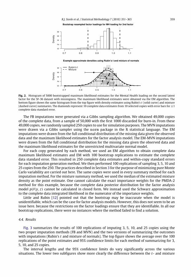
to limited and diffuse SSc patients with disease duration of 15 years or less who have completeinformation for the SF-36; there are 573 such subjects. We selected 230 subjects at random fromthe 573 and have made their subscale score for Mental Health and Role limitations due to emotionalproblem scoresmissing; the fraction of observationswithmissingness is approximately 40%.We focusour analyses on one of the factor loadings for the second factor in a factor analysis model that assumestwo latent factors following the same structure as suggested by the original SF-36 authors. The tophalf of Fig. 2 shows the resampled incomplete data maximum likelihood estimates of the MentalHealth factor loading for the second factor. We see that the incomplete data sampling distributionis left skewed, and so the asymptotic normal approximation might not be valid due to the missingobservations.
4.3. Simulation details
We examine four possible ways of generating copies of the missing data, namely:• proper imputation via draws from the posterior distribution generated via Gibbs sampling (FB),• proper imputation via single multivariate normal distribution and data augmentation (MVN),• improper imputation from the maximum likelihood estimates via the EM algorithm for the factoranalysis model with missing data (EM), and• improper imputation from the maximum likelihood estimate of the population covariance matrix(EM-MVN).
Fig. 2. Histogram of 5000 bootstrapped maximum likelihood estimates for the Mental Health loading on the second latentfactor for the SF-36 dataset with missingness. The maximum likelihood estimates were obtained via the EM algorithm. Thebottom figure shows the same histogram from the top figure with density estimates using Rubin’s t (solid curve) and mixture(dashed curve) summaries. The diamonds represent 10 complete data estimates from 10 selected copies with error bars for±1complete data standard error.
The FB imputations were generated via a Gibbs sampling algorithm. We obtained 49,000 copiesof the complete data, from a sample of 50,000 with the first 1000 discarded for burn-in. From these49,000 copies, we randomly sampled 250 copies to use for simulation purposes. TheMVN imputationswere drawn via a Gibbs sampler using the norm package in the R statistical language. The EMimputations were drawn from the full conditional distribution of the missing data given the observeddata and the maximum likelihood estimates for the factor analysis model. The EM-MVN imputationswere drawn from the full conditional distribution for the missing data given the observed data andthe maximum likelihood estimates for the unrestricted multivariate normal model.For each copy generated by each method, we used an EM algorithm to obtain complete data
maximum likelihood estimates and EM with 100 bootstrap replications to estimate the completedata standard error. This resulted in 250 complete data estimates and within-copy standard errorsfor each imputation generation method. We then performed 100 replications of sampling 3, 5, 10 and25 copies from the 250. The practices described in Section 3 for the purpose ofminimizing pureMonteCarlo variability are carried out here. The same copies were used in every summary method for eachimputationmethod. For the mixture summarymethod, we used the median of the estimatedmixturedensity as the point estimate. One cannot calculate the exact importance weights for the PMDA-2method for this example, because the complete data posterior distribution for the factor analysismodel p(θ |y, z) cannot be calculated in closed form. We instead used the Schwarz approximationto the complete data integrated likelihood in the numerator of the importance weights.Little and Rubin [12] pointed out that the bootstrap may be inaccurate when the model is
unidentifiable, which can be the case for factor analysis models. However, this does not seem to be anissue here. because the restrictions on the factor loadings ensure that they are identifiable. In all ourbootstrap replications, there were no instances where the method failed to find a solution.
4.4. Results
Fig. 3 summarizes the results of 100 replications of imputing 3, 5, 10, and 25 copies using thetwo proper imputation methods (FB and MVN) and the two versions of summarizing the outcomeswith imputations (Rubin’s t and mixture of normals). The top figure shows the average over the 100replications of the point estimates and 95% confidence limits for each method of summarizing for 3,5, 10, and 25 copies.The interval lengths and the 95% confidence limits do vary significantly across the various
situations. The lower two subfigures show more clearly the difference between the t- and mixture
Fig. 3. Quality of Life example: 100 replications of multiple imputation for two methods of summarizing (Rubin’s t [1, 2] andmixture of normals [3,4]) using copies of missing data generated from two different models (from the target factor analysisposterior distribution [1,3] and general multivariate normal [2,4]). The top subfigure shows the average of the estimates forthe Mental Health loading for the second latent factor (square or circle) and the associated 95% confidence limits (error bars)for the various methods of summarizing and generating form = 3, 5, 10, and 25 copies. The horizontal dashed lines show themaximum likelihood estimate and 95% confidence limits obtained from the non-parametric bootstrap. The lower-left subfigureshows the average interval width and the lower-right subfigure shows the standard deviation of the interval widths. In thelower-left subfigure, the horizontal dashed line is the interval width from the bootstrap sample.
summary methods. In general, the t-intervals are longer than the mixture summary intervals onaverage and the interval lengths are also more variable.We first focus on the results for the copies drawn from the fully Bayesian factor analysismodel (FB),
which correspond to the results labelled 1 (t-summaries) and 2 (mixture summaries). For 3, 5, 10, and25 copies respectively, the t-intervals are 25%, 11%, 4%, and 0.4% wider on average than the mixturesummary intervals. The t-intervals are much more variable in width than the mixture summaryintervals, as we also observed in the simulation study. The standard deviations of the t-intervals are3.1, 1.7 and 1.2 times larger than the standard deviations of themixture summary intervals for 3, 5 and10 copies respectively. For 25 copies, the t-intervals andmixture summary intervals are roughly equalin variability and both are similar in length to the bootstrap interval from the EM implementation forthe incomplete data set.The pattern is similar for copies drawn from the posterior for the general multivariate normal
model (MVN). The t-intervals are 27%, 11%, 4%, and 1% wider on average than the mixture intervalsfor 3, 5, 10, and 25 copies, while the t-interval widths are 2.7, 1.6, 1.2 and 1.0 times more variable.We also see that the intervals for theMVN copies are narrower than the intervals for copies generatedfrom the fully Bayesian model.In summary, multiple imputations from the full posterior distribution are theoretically more
accurate, and correspond more closely to the bootstrap than multivariate normal imputations
Fig. 4. Posterior density estimates for the Mental Health loading for the second factor using the Rubin’s t and the PMDA-1mixture summary approaches when imputing via 250 copies drawn from the Bayesian posterior distribution for the factoranalysis model. The gray solid line is the non-parametric density estimate from 5000 bootstrap samples, the black dashed lineis the summary using Rubin’s t-distribution, and the black solid line is the summary using a mixture of normals.
with larger numbers of copies. With fully Bayesian imputations, the mixture-based intervals aresubstantially narrower than the t-based intervals for small numbers of copies, converging when thenumber of copies reaches 25. The mixture-based intervals are also less variable than the t-basedintervals for small numbers of copies, again convergingwhen the number of copies reaches 25. Overall,fully Bayesian imputations with a mixture summary worked best in this example, particularly with10 or fewer copies.Fig. 4 shows density estimates using the t- and mixture summary methods for all 250 complete
data analyses generated from the posterior distribution for the factor analysis model. We comparethese to the density estimate from the 5000 non-parametric bootstrap resampled estimates using theEM algorithm for the incomplete data. With 250 copies, we can see that the mixture summaries areperforming better than the t-summary because of the ability tomodel the slight skew in the samplingdistribution of the factor loadings. The subfigures on the right side of the figure show that the t-summary underestimates the lower tail of the sampling distribution and overestimates the upper tail.In particular, in comparison to the mixture summary, the t-summary underestimates the area underthe curve of the left tails to the 2.5th and 5th percentiles by 27% and 14%, while it overestimates theequivalent right tails by 19% and 34% respectively. Thismay be due to the restriction of the t-summaryto a symmetric sampling (or posterior) distribution.We observe a slight bias in the estimation of the 95% confidence limits, although it is clear that
the mixture summary density is less biased than the t-summary density. The bias is likely due to tworeasons. First, the complete data posteriors for the factor loading, although less skewed, still exhibitsome skewness. This would prevent themixture of normals with a small number of copies from beingable to capture the skewed tail behavior. Second, the posterior distribution for the copies drawn fromthe fully Bayesian posterior distribution would depend on the priors used and different priors had
Fig. 5. 100 replications of multiple imputation for three methods of summarizing (Rubin’s t [1, 2], PMDA-1 [3,4], and PMDA-2 [5,6]) using copies of missing data generated from two different models (from a full conditional distribution based on theincomplete data factor analysis MLE [1,3,5] and theMLE from the general multivariate normal model [2,4,6]). The top subfigureshows the average of the estimates for theMentalHealth loading for the second latent factor (square or circle) and the associated95% confidence limits (error bars) for the various methods of summarizing and generating form = 3, 5, 10, and 25 copies. Thedashed lines across the width of the plot locate the maximum likelihood estimate and 95% confidence limits obtained from thenon-parametric bootstrap. The lower-left subfigure shows the average interval length and the lower-right subfigure shows thestandard deviation of the interval length. In the lower-left subfigure, the horizontal dashed line is the interval length from thebootstrap sample.
some effect on the shape and location of the posterior distribution (and thus on the copies of themissing data generated).Fig. 5 shows the results for the two improper copy generationmethods (EMand EM-MVN) for three
different summary methods (t-summary, mixture summary [PMDA-1], and importance weightedmixture summary [PMDA-2]). For the data generated using the EM approach, the t- and PMDA-1summary approaches behave similarly to the proper imputation methods. The t-intervals are 11%,6%, 2%, and 0.2% wider on average than the corresponding PMDA-1 intervals, for 3, 5, 10 and 25copies respectively. The standard deviations of the t-interval widths are 2.0, 1.5, 1.1 and 1.0 timesthe standard deviations of the PMDA-1 interval widths. So once again the t-intervals are less stablethan the equally weighted mixture summary intervals. Both summary methods yield intervals thatare much narrower on average than either of the proper imputation methods.We have also included results for an importance weighted mixture summary. The purpose of
the importance weights is to correct for the fact that we are sampling not from the true posteriordistribution of the missing data, but instead from an approximation that uses the incomplete datamaximum likelihood estimate.When the imputations were improperly generated, only PMDA-2 gaveacceptable outcomes. Even for PMDA-2, a moderate to large (m = 10 or 25) number of imputationcopies is needed to achieve roughly correct coverage. The average interval widths and stability of the
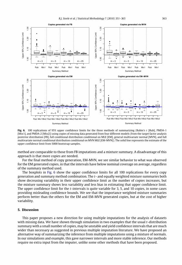
Fig. 6. 100 replications of 95% upper confidence limits for the three methods of summarizing (Rubin’s t [Rub], PMDA-1[Mix1], and PMDA-2 [Mix2]) using copies of missing data generated from four different models (from the target factor analysisposterior distribution [FB], full conditional distribution conditional on MLE [EM], general multivariate normal [MVN], and fullmultivariate normal conditional distribution conditional onMVNMLE [EM-MVN]). The solid line represents the estimate of theupper confidence limit from 5000 bootstrap samples.
method are comparable to those from FB imputations and a mixture summary. A disadvantage of thisapproach is that more copies are needed.For the final method of copy generation, EM-MVN, we see similar behavior to what was observed
for the EM generated copies, in that the intervals have below nominal coverage on average, regardlessof the summary method used.The boxplots in Fig. 6 show the upper confidence limits for all 100 replications for every copy
generation and summarymethod combination. The t- and equally weightedmixture summaries bothshow decreasing variability in their upper confidence limit as the number of copies increases, butthe mixture summary shows less variability and less bias in estimating that upper confidence limit.The upper confidence limit for the t-intervals is quite variable for 3, 5, and 10 copies, in some casesproviding misleading confidence bounds. We see that the importance weighted mixture summariesperform better than the others for the EM and EM-MVN generated copies, but at the cost of highervariability.
5. Discussion
This paper proposes a new direction for using multiple imputations for the analysis of datasetswith missing data. We have shown through simulation in two examples that the usual t-distributionsummarywith a small number of copies,may be unstable and yield confidence intervals that aremuchwider than necessary as suggested in previous multiple imputation literature. We have proposed analternative way of summarizing the inference frommultiple imputations using a mixture of normals.In our simulations and example, this gave narrower intervals andmore stable inference. Our methodsrequire no extra input from the imputer, unlike some other methods that have been proposed.
One could conclude that it is possible to improve on widely accepted methods for summarizingthe inference frommultiple imputation, such as Rubin’s t . Because of the extra variability introducedin the sampling of the missing observations from their true posterior distribution and the restrictionto using t-distributions for inference, multiple imputation with small to moderate numbers of copiescan provide inefficient or even incorrect inferences. Robins and Wang [16] looked at this problem indetail. Schafer and Schenker [22] cited this difficulty as a potential reason for using conditional meanimputation. Carabin et al. [3] gave an example of the failure of multiple imputation to yield usefulconfidence intervals in the context of censored regression models.Arguments similar to ours were made by Fay [5] and Rao and Shao [15] in their discussions of [20].
Rubin’s t estimators, in an effort to provide enough coverage,must inflate the variance of the completedata functionals to the pointwhere the estimates of the observed data functional become very variablethemselves. The estimated variability is often correct, but if the estimated variability is too high thenthe estimate could be of little use. It is important to note that the results investigated here apply onlyto small to moderate numbers of copies.Our approach could be viewed as a compromise between Rubin’s methods and the single
imputation methods of Fay [5] and Rao and Shao [15]. These single imputation methods usesophisticated methods to account for the uncertainty in parameter estimates while relying on thestability of a single, unbiased mean imputation to avoid the problems that multiple imputation haswhen drawing from the true posterior distribution. If one uses importance sampling methods likethose discussed here, approximately accurate estimates of variability can be obtained.We have approximated the complete data posterior distribution by a normal distribution, yielding
an approximation of the full posterior by amixture of normals, and found it toworkwell in simulationsand an example. It is possible that an even better approximationwould be provided by a t distribution,leading to an approximation of the posterior distribution by a mixture of t distributions. This wouldalso be more complicated, and an assessment of the resulting tradeoff between complexity andperformancewould be aworthy topic for further research. It should also be noted that doing inferenceon a scale where the normal approximation to the posterior is better is generally a good idea.In our experiments we found that good results are obtained by most methods with large numbers
of imputations. Thus the improvement from our methods over existing ones are likely to be greatestwhen the number of copies is small. This is most often the case when the copies are provided by theimputer rather than produced by the user. Increasing the number of copies produced is a good idea inany event when it is computationally feasible.The basic idea of approximating the posterior distribution in missing data cases by a mixture of
normals applies quite generally, but we have demonstrated it here only for scalar estimands. Theposterior distribution of a multivariate estimand can be approximated by our method by simplysimulating values of the parameters from the estimatedmixture of multivariate normal distributions.Detailed assessment of the application of the method to multivariate estimands and testing problemsis a topic for future research.A free R software package called MImix that implements our methods is available at http://cran.r-
project.org.
Acknowledgements
Steele’s research was supported by an NSERC Discovery Grant. Wang’s research was supportedby NIH grant CA 74552. Raftery’s research was supported by NIH grants R01 HD054511 and R01GM084163, NSF grants ATM 0724721 and IIS 0534094, and the Joint Ensemble Forecasting System(JEFS) under subcontract No. S06-47225 from the University Corporation for Atmospheric Research(UCAR). The authors acknowledge the Canadian Scleroderma Research Group (http://csrg-grcs.ca) andparticipating rheumatologists for the use for the CSRG SSc registry data. The authors are grateful tothe Guest Editor and two anonymous referees for their helpful comments.
References
[1] J. Barnard, D.B. Rubin, Small-sample degrees of freedom with multiple imputation, Biometrika 86 (1999) 948–955.[2] J.M. Bernardo, A.F.M. Smith, Bayesian Theory, John Wiley and Sons, 1994.
[3] H. Carabin, J. Gyorkos, J. Joseph, P. Payment, J. Soto, Comparison of methods to analyse imprecise faecal coliform countdata from environmental samples, Epidemiology and Infection 126 (2001) 1181–1190.
[4] M.D. Escobar, M. West, Bayesian density estimation and inference using mixtures, Journal of the American StatisticalAssociation 90 (1995) 577–588.
[5] R.E. Fay, Alternative paradigms for the analysis of imputed survey data, Journal of the American Statistical Association 91(1996) 490–498.
[6] T.S. Ferguson, Bayesian density estimation by mixtures of normal distributions, in: M.H. Rizvi, J.S. Rustagi, D. Siegmund(Eds.), Recent Advances in Statistics: Papers in Honor of Herman Chernoff on His Sixtieth Birthday, Academic Press, 1983,pp. 287–302.
[7] C. Fraley, A.E. Raftery, Model-based clustering, discriminant analysis, and density estimation, Journal of the AmericanStatistical Association 97 (2002) 611–631.
[8] J. Geweke, G. Zhou, Measuring the pricing error of the arbitrage pricing theory, The Review of Financial Studies 9 (1996)557–587.
[9] J. Jomeen, C.R. Martin, The factor structure of the SF-36 in early pregnancy, Journal of Psychosomatic Research 59 (2005)131–138.
[10] R.E. Kass, A.E. Raftery, Bayes factors, Journal of the American Statistical Association 90 (1995) 773–795.[11] S.D. Keller, J. Ware, P.M. Bentler, N.K. Aaronson, J. Alonso, G. Apolone, J.B. Bjorner, J. Brazier, M. Bullinger, S. Kaasa, A.
Leplège, M. Sullivan, B. Gandek, Use of structural equation modeling to test the construct validity of the SF-36 healthsurvey in ten countries: Results from the IQOLA project, Journal of Clinical Epidemiology 51 (1998) 1179–1188.
[12] R.J.A. Little, D.B. Rubin, Statistical analysis with missing data, 2nd ed., John Wiley and Sons, 2002.[13] H.F. Lopes, M. West, Bayesian model assessment in factor analysis, Statistica Sinica 14 (2004) 41–67.[14] X.-L. Meng, Missing data: Dial M for ???, Journal of the American Statistical Association 95 (452) (2000) 1325–1330.[15] J.N.K. Rao, J. Shao, On balanced half-sample variance estimation in stratified random sampling, Journal of the American
Statistical Association 91 (1996) 343–348.[16] J.M. Robins, N. Wang, Inference for imputation estimators, Biometrika 87 (2000) 113–124.[17] K. Roeder, L. Wasserman, Practical Bayesian density estimation using mixtures of normals, Journal of the American
Statistical Association 92 (1997) 894–902.[18] D.B. Rubin, Multiple imputations in sample surveys: A phenomenological Bayesian approach to nonresponse, in: ASA
Proceedings of the Section on Survey Research Methods, 1978, pp. 20–28.[19] D.B. Rubin, Multiple imputation for nonresponse in surveys, John Wiley and Sons, 1987.[20] D.B. Rubin, Multiple imputation after 18+ years, Journal of the American Statistical Association 91 (1996) 473–489.[21] J.L. Schafer, Analysis of incomplete multivariate data, Chapman & Hall Ltd, London, 1997.[22] J.L. Schafer, N. Schenker, Inference with imputed conditional means, Journal of the American Statistical Association 95
(2000) 144–154.[23] G. Schwarz, Estimating the dimension of a model, Annals of Statistics 6 (1978) 461–464.[24] J. Ware, B. Gandek, Overview of the SF-36 health survey and the international quality of life assessment (IQOLA) project,
Journal of Clinical Epidemiology 51 (1998) 903–912.[25] J. Ware, M. Kosinski, SF-36 physical and mental health summary scales: A manual for users of version 1’’, second ed.,
QualityMetric Incorporated, Lincoln, RI, 2001.[26] J. Ware, M. Kosinski, B. Gandek, N.K. Aaronson, G. Apolone, P. Bech, J. Brazier, M. Bullinger, S. Kaasa, A. Leplge, L. Prieto,
M. Sullivan, The factor structure of the SF-36 health survey in 10 countries: Results from the IQOLA project, Journal ofClinical Epidemiology 51 (1998) 1159–1165.
[27] G.C.G. Wei, M.A. Tanner, A Monte Carlo implementation of the EM algorithm and the Poor Man’s Data Augmentationalgorithms, Journal of the American Statistical Association 85 (1990) 699–704.
[28] M. West, Approximating posterior distributions by mixtures, Journal of the Royal Statistical Society, Series B,Methodological 55 (1993) 409–422.
[29] C.-H. Wu, K.-L. Lee, G. Yao, Examining the hierarchical factor structure of the SF-36 Taiwan version by exploratory andconfirmatory factor analysis, Journal of Evaluation in Clinical Practice 13 (2007) 889–900.