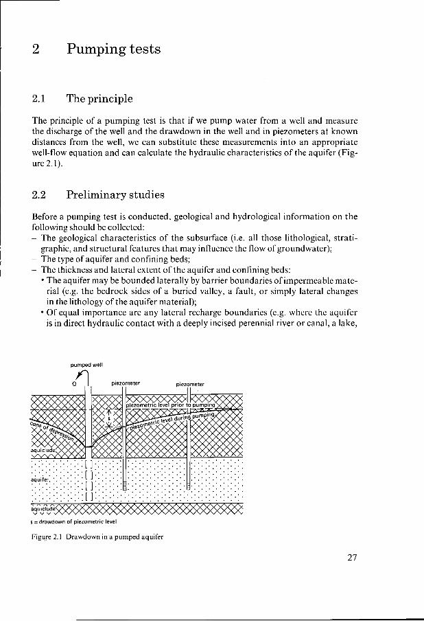
Figure 2.1 Drawdown in a pumped aquifer pumped well piezometer piezometer . . . . . . . . . . . . .. . . . . . . . . .[ ]:.'.'.'.'. :: ~.'.~.~.~.~.'.~.~.~.'.~.'.~.' . . . . . . . .... .............. ........ ..... .............. s =drawdown of piezometric level 2 Pumping tests 2.1 The principle The principle of a pumping test is that if we pump water from a well and measure the discharge of the well and the drawdown in the well and in piezometers at known distances from the well, we can substitute these measurements into an appropriate well-flow equation and can calculate the hydraulic characteristics of the aquifer (Fig- ure 2.1). 2.2 Preliminary studies Before a pumping test is conducted, geological and hydrological information on the following should be collected: - The geological characteristics of the subsurface (i.e. all those lithological, strati- - The type of aquifer and confining beds; - The thickness and lateral extent of the aquifer and confining beds: graphic, and structural features that may influence the flow of groundwater); The aquifer may be bounded laterally by barrier boundaries of impermeable mate- rial (e.g. the bedrock sides of a buried valley, a fault, or simply lateral changes in the lithology of the aquifer material); Of equal importance are any lateral recharge boundaries (e.g. where the aquifer is in direct hydraulic contact with a deeply incised perennial river or canal, a lake, 27
The principle of a pumping test is that if we pump water from a well and measure the discharge of the well and the drawdown in the well and in piezometers at known distances from the well, we can substitute these measurements into an appropriate well-flow equation and can calculate the hydraulic characteristics of the aquifer (Fig- ure 2.1).
2.2 Preliminary studies
Before a pumping test is conducted, geological and hydrological information on the following should be collected: - The geological characteristics of the subsurface (i.e. all those lithological, strati-
- The type of aquifer and confining beds; - The thickness and lateral extent of the aquifer and confining beds:
graphic, and structural features that may influence the flow of groundwater);
The aquifer may be bounded laterally by barrier boundaries of impermeable mate- rial (e.g. the bedrock sides of a buried valley, a fault, or simply lateral changes in the lithology of the aquifer material); Of equal importance are any lateral recharge boundaries (e.g. where the aquifer is in direct hydraulic contact with a deeply incised perennial river or canal, a lake,
27
or the ocean) or any horizontal recharge boundaries (e.g. where percolating rain or irrigation water causes the watertable of an unconfined aquifer to rise, or where an aquitard leaks and recharges the aquifer);
- Data on the groundwater-flow system: horizontal or vertical flow of groundwater, watertable gradients, and regional trends in groundwater levels;
- Any existing wells in the area. From the logs of these wells, it may be possible to derive approximate values of the aquifer’s transmissivity and storativity and their spatial variation. It may even be possible to use one of those wells for the test, thereby reducing the cost of field work. Sometimes, however, such a well may pro- duce uncertain results because details of its construction and condition are not avail- able.
2.3 Selecting the site for the well .
When an existing well is to be used for the test or when the hydraulic characteristics of a specific location are required, the well site is predetermined and one cannot move to another, possibly more suitable site. When one has the freedom to choose, however, the following points should be kept in mind: - The hydrogeological conditions should not change over short distances and should
be representative of the area under consideration, or at least a large part of it; - The site should not be near railways or motorways where passing trains or heavy
traffic might produce measurable fluctuations in the hydraulic head of a confined aquifer;
- The site should not be in the vicinity of existing discharging wells; - The pumped water should be discharged in a way that prevents its return to the
- The gradient of the watertable or piezometric surface should be low; - Manpower and equipment must be able to reach the site easily.
aquifer;
2.4 The well
After the well site has been chosen, drilling operations can begin. The well will consist of an open-ended pipe, perforated or fitted with a screen in the aquifer to allow water to enter the pipe, and equipped with a pump to lift the water to the surface. For the design and construction of wells, we refer to Driscoll (1986), Groundwater Manual (1981), and Genetier (1984), where full details are given. Some of the major points are summarized below.
2.4.1 Well diameter
A pumping test does not require expensive large-diameter wells. If a suction pump placed on the ground surface is used, as in shallow watertable areas, the diameter of the well can be small. A submersible pump requires a well diameter large enough to accommodate the pump.
28
The diameter of the well can be varied without greatly affecting the yield of the well. Doubling the diameter would only increase the yield by about 10 per cent, other things being equal.
2.4.2 Well depth
The depth of the well will usually be determined from the log of an exploratory bore hole or from the logs of nearby existing wells, if any. The well should be drilled to the bottom of the aquifer, if possible, because this has various advantages, one of which is that it allows a longer well screen to be placed, which will result in a higher well yield.
During drilling operations, samples of the geological formations that are pierced should be collected and described lithologically. Records should be kept of these litho- logical descriptions, and the samples themselves should be stored for possible future reference.
2.4.3 Well screen
The length of the well screen and the depth at which it is placed will largely be decided by the depth at which the coarsest materials are found. In the lithological descriptions, therefore, special attention should be given to the grain size of the various materials. If geophysical well logs are run immediately after the completion of drilling, a prelimin- ary interpretation of those logs will help greatly in determining the proper depth a t which to place the screen.
If the aquifer consists of coarse gravel, the screen can be made locally by sawing, drilling, punching, or cutting openings in the pipe. In finer formations, finer openings are needed. These may vary in size from some tenths of a millimetre to several milli- metres. Such precision-made openings can only be obtained in factory-made screens. To prevent the blocking of well screen openings by spherical grains, long narrow slits are preferable. The slots should retain 30 to 50 per cent of the aquifer material, depend- ing on the uniformity coefficient of the aquifer sample. (For details, see Driscoll 1986; Huisman 1972.)
The well screen should be slotted or perforated over no more than 30 to 40 per cent of its circumference to keep the entrance velocity low, say less than about 3 cm/s. At this velocity, the friction losses in the screen openings are small and may even be negligible.
A general rule is to screen the well over at least 80 per cent of the aquifer thickness because this makes it possible to obtain about 90 per cent or more of the maximum yield that could be obtained if the entire aquifer were screened. Another even more important advantage of this screen length is that the groundwater flow towards the well can be assumed to be horizontal, an assumption that underlies almost all well-flow equations (Figure 2.2A). There are some exceptions to the general rule: - In unconfined aquifers, it is common practice to screen only the lower half or lower
one-third of the aquifer because, if appreciable drawdowns occur, the upper part
29
A B fully partially penetrating penetrating well well
Figure 2.2 A) A fully penetrating well; B) A partially penetrating well
of a longer well screen would fall dry; - In a very thick aquifer, it will be obvious that the length of the screen will have
to be less than 80 per cent, simply for reasons of economy. Such a well is said to be a partially penetrating well. It induces vertical-flow components, which can extend outwards from the well to distances roughly equal to 1.5 times the thickness of the aquifer (Figure 2.2B). Within this radius, the measured drawdowns have to be corrected before they can be used in calculating the aquifer characteristics;
- Wells in consolidated aquifers do not need a well screen because the material around the well is stable.
2.4.4 Gravel pack
It is easier for water to enter the well if the aquifer material immediately surrounding the screen is removed and replaced by artificially-graded coarser material. This is known as a gravel pack. When the well is pumped, the gravel pack will retain much of the aquifer material that would otherwise enter the well. With a gravel pack, larger slot sizes can be selected for the screen. The thickness of the pack should be in the range of 8 to 15 cm. Gravel pack material should be clean, smoothly-rounded grains. Details on the gravel sizes to be used in gravel packs are given by Driscoll (1986) and Huisman (1972).
2.4.5 The pump
After the well has been drilled, screened, and gravel-packed, as necessary, a pump has to be installed to lift the water. It is beyond the scope of this book to discuss
30
the many kinds of pumps that might be used, so some general remarks must suffice: - The pump and power unit should be capable of operating continuously at a constant
discharge for a period of at least a few days. An even longer period may be required for unconfined or leaky aquifers, and especially for fractured aquifers. The same applies if drawdown data from piezometers at great distances from the well are to be analyzed. In such cases, pumping should continue for several days more;
- The capacity of the pump and the rate of discharge should be high enough to produce good measurable drawdowns in piezometers as far away as, say, 1 O0 or 200 m from the well, depending on the aquifer conditions.
After the pump has been installed, the well should be developed by being pumped a t a low discharge rate. When the initially cloudy water becomes clear, the discharge rate should be increased and pumping continued until the water clears again. This procedure should be repeated until the desired discharge rate for the test is reached or exceeded.
2.4.6 Discharging the pumped water
The water delivered by the well should be prevented from returning to the aquifer. This can be done by conveying the water through a large-diameter pipe, say over a distance of 100 or 200 m, and then discharging it into a canal or natural channel. The water can also be conveyed through a shallow ditch, but the bottom of the ditch should be sealed with clay or plastic sheets to prevent leakage. Piezometers can be used to check whether any water is lost through the bottom of the ditch.
2.5 Piezometers
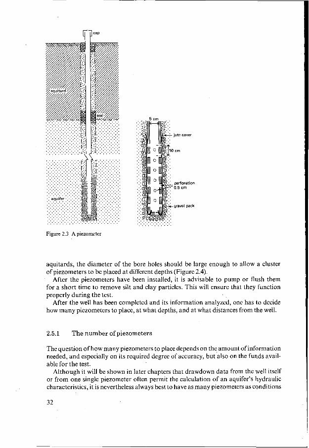
A piezometer (Figure 2.3) is an open-ended pipe, placed in a borehole that has been drilled to the desired depth in the ground. The bottom tip of the piezometer is fitted with a perforated or slotted screen, 0.5 to 1 m long, to allow the inflow of water. A plug at the bottom and jute or cotton wrapped around the screen will prevent the entry of fine aquifer material.
The annular space around the screen should be filled with a gravel pack or uniform coarse sand to facilitate the inflow of water. The rest of the annular space can be filled with any material available, except where the presence of aquitards requires a seal of bentonite clay or cement grouting to prevent leakage along the pipe. Experience has taught us that very fine clayey sand provides almost as good a seal as bentonite. It produces an error of less than 0.03 m, even when the difference in head between the aquifers is more than 30 m.
The water levels measured in piezometers represent the average head at the screen of the piezometers. Rapid and accurate measurements can best be made in small- diameter piezometers. If their diameter is large, the volume of water contained in them may cause a time lag in changes in drawdown. When the depth to water is to be mea- sured manually, the diameter of the piezometers need not be larger than 5 cm. If auto- matic water-level recorders or electronic water pressure transducers are used, larger- diameter piezometers will be needed. In a heterogeneous aquifer with intercalated
aquitards, the diameter of the bore holes should be large enough to allow a cluster of piezometers to be placed at different depths (Figure 2.4).
After the piezometers have been installed, it is advisable to pump or flush them for a short time to remove silt and clay particles. This will ensure that they function properly during the test.
After the well has been completed and its information analyzed, one has to decide how many piezometers to place, at what depths, and at what distances from the well.
2.5.1 The number of piezometers
The question of how many piezometers to place depends on the amount ofinformation needed, and especially on its required degree of accuracy, but also on the funds avail- able for the test.
Although it will be shown in later chapters that drawdown data from the well itself or from one single piezometer often permit the calculation of an aquifer’s hydraulic characteristics, it is nevertheless always best to have as many piezometers as conditions
32
permit. Three, at least, are recommended. The advantage of having more than one piezometer is that the drawdowns measured in them can be analyzed in two ways: by the time-drawdown relationship and by the distance-drawdown relationship. Obviously, the results of such analyses will be more accurate and will be representative of a larger volume of the aquifer.
2.5.2 Their distance from the well
Piezometers should be placed not too near the well, but not too far from it either. This rather vague statement needs some explanation. So,, as will be outlined below, the distances at which piezometers should be placed depends on the type of aquifer, its transmissivity, the duration of pumping, the discharge rate, the length of the well screen, and whether the aquifer is stratified or fractured.
The type of aquifer When a confined aquifer is pumped, the loss of hydraulic head propagates rapidly because the release of water from storage is entirely due to the compressibility of the aquifer material and that of the water. The drawdown will be measurable a t great distances from the well, say several hundred metres or more.
In unconfined aquifers, the loss of head propagates slowly. Here, the release of water from storage is mostly due to the dewatering of the zone through which the
cluster of pumped well piezometers
Figure 2.4 Cluster of piezometers in a heterogeneous aquifer intercalated with aquitards
33
water is moving, and only partially due to the compressibility of the water and aquifer material. Unless pumping continues for several days, the drawdown will only be mea- surable fairly close to the well, say not much more than about 100 m.
A leaky aquifer occupies an intermediate position. Depending on the hydraulic resis- tance of its confining aquitard (or aquitards), a leaky aquifer will resemble either a confined or an unconfined aquifer.
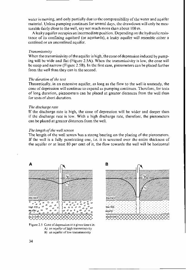
Transmissivity When the transmissivity of the aquifer is high,the cone of depression induced by pump- ing will be wide and flat (Figure 2.5A). When the transmissivity is low, the cone will be steep and narrow (Figure 2.5B). In the first case, piezometers can be placed farther from the well than they can in the second.
The duration of the test Theoretically, in an extensive aquifer, as long as the flow to the well is unsteady, the cone of depression will continue to expand as pumping continues. Therefore, for tests of long duration, piezometers can be placed at greater distances from the well than for tests of short duration.
The discharge rate If the discharge rate is high, the cone of depression will be wider and deeper than if the discharge rate is low. With a high discharge rate, therefore, the piezometers can be placed at greater distances from the well.
The length of the well screen The length of the well screen has a strong bearing on the placing of the piezometers. If the well is a fully penetrating one, i.e. it is screened over the entire thickness of the aquifer or at least 80 per cent of it, the flow towards the well will be horizontal
O [ ] O o o o 0 low KD: : : , ' : : :[ 1.. : : : : : : : : . a q u i f e r ' . ' . ' . ' . ' . ' . ' . [ I : . ' . ' . ' . . . . . . ' " " . 0 0 0 . . . . . . . . . . . . . . . . . . .
. . . . . . . . . . . . . . . . . . o " o u D D o[ O O 0 D
Figure 2.5 Cone of depression at a given timet in: A) an aquifer of high transmissivity B) an aquifer of low transmissivity
34
and piezometers can be placed close to the well. Obviously, if the aquifer is not very thick, it is always best to employ a fully penetrating well.
If the well is only partially penetrating, the relatively short length of well screen will induce vertical flow components, which are most noticeable near the well. If piez- ometers are placed near the well, their water-level readings will have to be corrected before being used in the analysis. These rather complicated corrections can be avoided if the piezometers are placed farther from the well, say at distances which are at least equal to 1.5 times the thickness of the aquifer. At such distances, it can be assumed that the flow is horizontal (see Figure 2.2) .
Stra t $ca tion Homogeneous aquifers seldom occur in nature, most aquifers being stratified to some degree. Stratification causes differences in horizontal and vertical hydraulic conductiv- ity, so that the drawdown observed at a certain distance from the well may differ at different depths within the aquifer. As pumping continues, these differences in draw- down diminish. Moreover, the greater the distance from the well, the less effect stratifi- cation has upon the drawdowns.
Fractured rock Deciding on the number and location of piezometers in fractured rock poses a special problem, although the rock can be so densely fractured that its drawdown response to pumping resembles that of an unconsolidated homogeneous aquifer; if so, the number and location of the piezometers can be chosen in the same way as for such an aquifer.
If the fracture is a single vertical fracture, however, matters become more compli- cated. The number and location of piezometers will then depend on the orientation of the fracture (which may or may not be known) and on the transmissivity of the rock on opposite sides of the fracture (which may be the same or, as so often happens, is not the same). Further, the fracture may be open or closed. If it is open, its hydraulic conductivity can be regarded as infinite, and it will resemble a canal whose water level is suddenly lowered. There will then be no hydraulic gradient inside the fracture, so that it can be regarded as an ‘extended well’, or as a drain that receives water from the adjacent rock through parallel flow. This situation requires that piezometers be placed along a line perpendicular to the fracture. To check whether the fracture can indeed be regarded as an ‘extended well’, a few piezometers should be placed in the fracture itself.
If the hydraulic conductivity of the fracture is severely reduced by weathering or by the deposition of minerals on the fracture plane, pumping will cause hydraulic gradients to develop in the fracture and in the adjacent rock. This situation requires piezometers in the fracture and in the adjacent rock.
If the fracture is a single vertical open fracture of infinite hydraulic conductivity and known orientation, and if the transmissivity of the rock is the same on both sides of the fracture, two piezometers on the same side of the fracture are required to deter- mine the perpendicular distances between the piezometers and the fracture (Figure 2.6A). In this figure, the piezometer closest to the pumped well is not the piezometer closest to the fracture. Regardless of the distances r, and rz, the drawdown will be greatest in the piezometer closest to the fracture. To analyze pumping test data from
35
such a fracture, we must know the distances between the piezometers and the fracture, xI and x2, which we can calculate from r, and r2, measured in the field, and the angles O, and 02.
If the precise orientation of the fracture is not known, more than two piezometers will be needed. As can be seen in Figure 2.6B, if x1 is small relative to x2, two orienta- tions are possible because xI may be on either side of the fracture. More piezometers must then be placed to find the orientation.
More piezometers are also required if there is geological evidence that the transmissi- vity of the rock on opposite sides of the fracture is significantly different.
Summarizing As is obvious from the above, there are many factors to be taken into account in deciding how far from the well the piezometers should be placed. Nevertheless, if one has a proper knowledge of the test site (especially of the type of aquifer, its thickness, stratification or fracturing, and expected transmissivity), it will be easier to make the right decisions.
Although no fixed rule can be given and the ultimate choice depends entirely on local conditions, placing piezometers between 10 and 100 m from the well will give reliable data in most cases. For thick aquifers or stratified confined ones, the distances should be greater, say between 1 O0 and 250 m or more from the well.
One or more piezometers should also be placed outside the area affected by the pumping so that the natural behaviour of the hydraulic head in the aquifer can be
A piezometer 1
J
, ./
,0 z m p e d well /
0 /
0 0
0 0
6 piezometer 2
0
'0 pumped well /
0 /
0 0
0 0
Figure 2.6 Piezometer arrangement near a fracture: A) of known orientation B) of unknown orientation
36
L O 0
LIO m 4 30 m P
P P 600m
loom 4
Figure 2.7 Example of a piezometer arrangement
measured. These piezometers should be several hundred metres away ,,om the well, or in the case of truly confined aquifers, as far away as one kilometre or more. If the readings from these piezometers show water-level changes during the test (e.g. changes caused by natural discharge or recharge), these data will be needed to correct the drawdowns induced by the pumping.
An example of a piezometer arrangement in an unconsolidated leaky aquifer is shown in Figure 2.7.
2.5.3 Depth of the piezometers
The depth of the piezometers is at least as important as their distance from the well. In an isotropic and homogeneous aquifer, the piezometers should be placed at a depth that coincides with that of half the length of the well screen. For example, if the well is fully penetrating and its screen is between 10 and 20 m below the ground surface, the piezometers should be placed at a depth of about 15 m.
For heterogeneous aquifers made up of sandy deposits intercalated with aquitards, it is recommended that a cluster of piezometers be placed, i.e. one piezometer in each sandy layer (see Figure 2.4). The holes in the aquitards should be sealed to prevent leakage along the tubes. Despite these precautions, some leakage may still occur, so it is recommended that the screens be placed a few metres away from the upper and lower boundaries of the aquitards where the effect of this leakage is small.
If an aquifer is overlain by a partly saturated aquitard, piezometers should also be placed in the aquitard to check whether its watertable is affected when the underly- ing aquifer is pumped. This information is needed for the analysis of tests in leaky aquifers.
2.6 The measurements to be taken
The measurements to be taken during a pumping test are of two kinds: - Measurements of the water levels in the well and the piezometers;
37
- Measurements of the discharge rate of the well. Ideally, a pumping test should not start before the natural changes in hydraulic head in the aquifer are known - both the long-term regional trends and the short-term local variations. So, for some days prior to the test, the water levels in the well and the piezometers should be measured, say twice a day. If a hydrograph (i.e. a curve of time versus water level) is drawn for each of these observation points, the trend and rate of water-level change can be read. At the end of the test (i.e. after complete recovery), water-level readings should continue for one or two days. With these data, the hydrographs can be completed and the rate of natural water-level change during the test can be determined. This information can then be used to correct the drawdowns observed during the test.
Special problems arise in coastal aquifers whose hydraulic head is affected by tidal movements. Prior to the test, a complete picture of the changes in head should be obtained, including maximum and minimum water levels in each piezometer and their time of occurrence.
When a test is expected to last one or more days, measurements should also be made of the atmospheric pressure, the levels of nearby surface waters, if present, and any precipitation.
In areas where production wells are operating, the pumping test has to be conducted under less than ideal conditions. Nevertheless, the possibly significant effects of these interfering wells can be eliminated from the test data if their on-off times and discharge rates are monitored, both before and during the test. Even so, it is best to avoid the disturbing influence of such wells if at all possible.
2.6.1 Water-level measurements
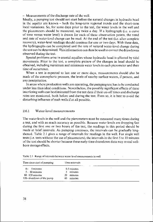
The water levels in the well and the piezometers must be measured many times during a test, and with as much accuracy as possible. Because water levels are dropping fast during the first one or two hours of the test, the readings in this period should be made a t brief intervals. As pumping continues, the intervals can be gradually leng- thened. Table 2.1 gives a range of intervals for readings in the well. For single well tests (i.e. tests without the use of piezometers), the intervals in the first 5 to 10 minutes of the test should be shorter because these early-time drawdown data may reveal well- bore storage effects.
Table 2.1 Range of intervals between water-level measurements in well
Time since start of pumping Time intervals
O- 5minutes 0.5 minutes 5- 60minutes 5 minutes
60- 120 minutes 20 minutes 120-shutdown of the pump 60 minutes
38
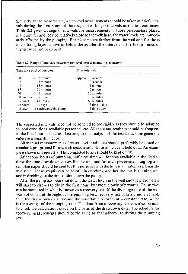
Similarly, in the piezometers, water-level measurements should be taken at brief inter- vals during the first hours of the test, and at longer intervals as the test continues. Table 2.2 gives a range of intervals for measurements in those piezometers placed in the aquifer and located relatively close to the well; here, the water levels are immedi- ately affected by the pumping. For piezometers farther from the well and for those in confining layers above or below the aquifer, the intervals in the first minutes of the test need not be so brief.
Table 2.2 Range of intervals between water-level measurements in piezometers
Time since start of pumping Time intervals
O - 2minutes 2 - Sminutes 5 - 15 minutes
15 - Sominutes 50 - 100 minutes
100 minutes - 5 hours 5 hours - 48 hours
48 hours - 6days 6days -shutdown of the pump
approx. I O seconds 30 seconds
1 minute 5 minutes
I O minutes 30 minutes 60 minutes
3 times a day 1 time a day
The suggested intervals need not be adhered to too rigidly as they should be adapted to local conditions, available personnel, etc. All the same, readings should be frequent in the first hours of the test because, in the analysis of the test data, time generally enters in a logarithmic form.
All manual measurements of water levels and times should preferably be noted on standard, pre-printed forms, with space available for all relevant field data. An exam- ple is shown in Figure 2.8. The completed forms should be kept on file.
After some hours of pumping, sufficient time will become available in the field to draw the time-drawdown curves for the well and for each piezometer. Log-log and semi-log paper should be used for this purpose, with the time in minutes on a logarith- mic scale. These graphs can be helpful in checking whether the test is running well and in deciding on the time to shut down the pump.
After the pump has been shut down, the water levels in the well and the piezometers will start to rise - rapidly in the first hour, but more slowly afterwards. These rises can be measured in what is known as a recovery test. If the discharge rate of the well was not constant throughout the pumping test, recovery-test data are more reliable than the drawdown data because the watertable recovers at a constant rate, which is the average of the pumping rate. The data from a recovery test can also be used to check the calculations made on the basis of the drawdown data. The schedule for 'recovery measurements should be the same as that adhered to during the pumping test.
39
Pumping t e s t ~ ~ . ~ . S r . E . O . ~ . ~ ~ E ~ ,
Pumping test by ....... !.&.kV ..................... Directed by ......... H.:.,w. For project . .A.cYz. E K ................. Location .... .V . f iE .6 .4 L.?X.N .....
..................
!.!h.? ........
Initial water level .....
Final water level .......... !..~...?%. Reference level ,~~.P. . !?.~. , !% Fi ....................... = 2?.32?. +m.S.l.*
TE.? ................................................................................ n. .czIS/l\n/P.Wh!. L.N.. .Grl.. ............................. ................ .WA.TE!Y..
Figure 2.8 Example of a pre-printed pumping-test form
2.6.1.1 Water-level-measuring devices
The most accurate recordings of water-level changes are made with fully-automatic microcomputer-controlled systems, as developed, for instance, by the TNO Institute of Applied Geoscience, The Netherlands (Figure 2.9). This system uses pressure trans-, ducers or acoustic transducers for continuous water-level recordings, which are stored on magnetic tape (see also Kohlmeier et al. 1983).
A good alternative is the conventional automatic recorder, which also produces a continuous record of water-level changes. Such recorders, however, require large- diameter piezometers.
40
, Fairly accurate measurements can be taken by hand, but then the instant of each reading must be recorded with a chronometer. Experience has shown that i t is possible to measure water levels to within 1 or 2 mm with one of the following: - A floating steel tape and standard with pointer; - An electrical sounder; - The wetted-tape method. For piezometers close to the well where water levels are changing rapidly during the first hours of the test, the most convenient device is the floating steel tape with pointer because it permits direct readings. For piezometers far from the well, conventional automatic recorders are the most suitable devices because only slow water-level changes can be interpreted from their graphs. For piezometers at intermediate dis- tances, either floating or hand-operated water-level indicators can be used, but even when water levels are changing rapidly, accurate observations can be made with a recorder, provided a chronometer is used and the time of each reading is marked manually on the graph.
For detailed descriptions of automatic recorders, mechanical and electrical sounders, and other equipment for measuring water levels in wells, we refer to hand- books (e.g. Driscoll 1986; Genetier 1984; Groundwater Manual 1981).
2.6.2 Discharge-rate measurements
Amongst the arrangements to be made for a pumping test is a proper control of the discharge rate. This should preferably be kept constant throughout the test. During pumping, the discharge should be measured at least once every hour, and any necessary adjustments made to keep it constant.
Figure 2.9 A fully-automated micro-computer-controlled recorder
41
The discharge can be kept constant by a valve in the discharge pipe. This is a more accurate method of control than changing the speed of the pump.
The fully-automatic computer-controlled system shown earlier in Figure 2.9 includes a magnetic flow meter for discharge measurements as part of a discharge- correction scheme to maintain a constant discharge.
A constant discharge rate, however, is not a prerequisite for the analysis of a pump- ing test. There are methods available that take variable discharge into account, whether it be due to natural causes or is deliberately provoked.
2.6.2.1 Discharge-measuring devices ,
To measure the discharge rate, a commercial water meter of appropriate capacity can be used. The meter should be connected to the discharge pipe in a way that ensures accurate readings being made: at the bottom of a U-bend, for instance, so that the pipe is running full., If the water is being discharged through a small ditch, a flume can be used to measure the discharge.
If no appropriate water meter or flume is available, there are other methods of measuring or estimating the discharge.
Container A very simple and fairly accurate method is to measure the time it takes to fill a contain- er of known capacity (e.g. an oil drum). This method can only be used if the discharge rate is low.
Orifice weir The circular orifice weir is commonly used to measure the discharge from a turbine or centrifugal pump. It does not work when a piston pump is used because the flow from such a pump pulsates too much.
The orifice is a perfectly round hole in the centre of a circular steel plate which is fastened to the outer end of a level discharge pipe. A piezometer tube is fitted in a 0.32 or 0.64 cm hole made in the discharge pipe, exactly 61 cm from the orifice plate. The water level in the piezometer represents the pressure in the discharge pipe when water is pumped through the orifice. Standard tables have been published which show the flow rate for various combinations of orifice and pipe diameter (Driscoll 1986).
Orifice bucket The orifice bucket was developed in the U.S.A. It consists of a small cylindrical tank with circular openings in the bottom. The water from the pump flows into the tank and discharges through the openings. The tank fills with water to a level where the pressure head causes the outflow through the openings to equal the inflow from the pump. If the tank overflows, one or more orifices are opened. If the water in the tank does not rise sufficiently, one or more orifices are closed with plugs.
A piezometer tube is connected to the outer wall of the tank near the bottom, and a vertical scale is fastened behind the tube to allow accurate readings of the water level in the tank. A calibration curve is required, showing the rate of discharge through
42
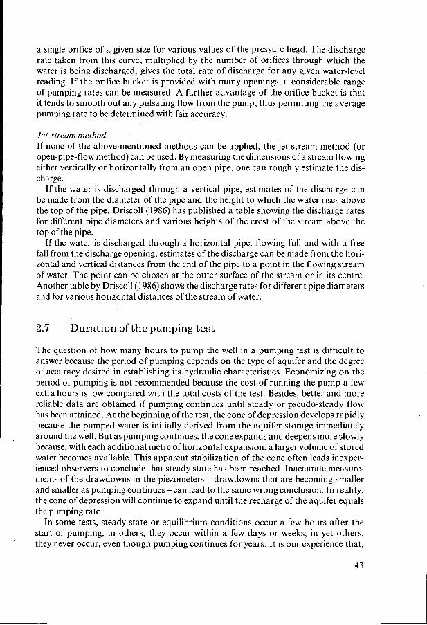
a single orifice of a given size for various values of the pressure head. The discharge rate taken from this curve, multiplied by the number of orifices through which the water is being discharged, gives the total rate of discharge for any given water-level reading. If the orifice bucket is provided with many openings, a considerable range of pumping rates can be measured. A further advantage of the orifice bucket is that it tends to smooth out any pulsating flow from the pump, thus permitting the average pumping rate to be determined with fair accuracy.
Jet-stream method If none of the above-mentioned methods can be applied, the jet-stream method (or open-pipe-flow method) can be used. By measuring the dimensions of a stream flowing either vertically or horizontally from an open pipe, one can roughly estimate the dis- charge.
If the water is discharged through a vertical pipe, estimates of the discharge can be made from the diameter of the pipe and the height to which the water rises above the top of the pipe. Driscoll (1986) has published a table showing the discharge rates for different pipe diameters and various heights of the crest of the stream above the top of the pipe.
If the water is discharged through a horizontal pipe, flowing full and with a free fall from the discharge opening, estimates of the discharge can be made from the hori- zontal and vertical distances from the end of the pipe to a point in the flowing stream of water. The point can be chosen at the outer surface of the stream or in its centre. Another table by Driscoll(l986) shows the discharge rates for different pipe diameters and for various horizontal distances of the stream of water.
2.7 Duration of the pumping test
The question of how many hours to pump the well in a pumping test is difficult to answer because the period of pumping depends on the type of aquifer and the degree of accuracy desired in establishing its hydraulic characteristics. Economizing on the period of pumping is not recommended because the cost of running the pump a few extra hours is low compared with the total costs of the test. Besides, better and more reliable data are obtained if pumping continues until steady or pseudo-steady flow has been attained. At the beginning of the test, the cone of depression develops rapidly because the pumped water is initially derived from the aquifer storage immediately around the well. But as pumping continues, the cone expands and deepens more slowly because, with each additional metre of horizontal expansion, a larger volume of stored water becomes available. This apparent stabilization of the cone often leads inexper- ienced observers to conclude that steady state has been reached. Inaccurate measure- ments of the drawdowns in the piezometers - drawdowns that are becoming smaller and smaller as pumping continues - can lead to the same wrong conclusion. In reality, the cone of depression will continue to expand until the recharge of the aquifer equals the pumping rate.
In some tests, steady-state or equilibrium conditions occur a few hours after the start of pumping; in others, they occur within a few days or weeks; in yet others, they never occur, even though pumping continues for years. It is our experience that,
43
under average conditions, a steady state is reached in leaky aquifers after 15 to 20 hours of pumping; in a confined aquifer, it is good practice to pump for 24 hours; in an unconfined aquifer, because the cone of depression expands slowly, a longer period is required, say 3 days.
As will be demonstrated in later chapters, it is not absolutely necessary to continue pumping until a steady state has been reached, because methods are available to ana- lyze unsteady-state data. Nevertheless, it is good practice to strive for a steady state, especially when accurate information on the aquifer characteristics is desired, say as a basis for the construction of a pumping station for domestic water supplies or other expensive works. If a steady state has been reached, simple equations can be used to analyze the data and reliable results will be obtained. Besides, the longer period of pumping required to reach steady state may reveal the presence of boundary condi- tions previously unknown, or in cases of fractured formations, will reveal the specific flows that develop during the test.
Preliminary plotting of drawdown data during the test will often show what is hap- pening and may indicate how much longer the test should continue.
2.8 Processing the data
2.8.1 Conversion of the data
The water-level data collected before, during, and after the test should first be expressed in appropriate units. The measurement units of the International System are recommended (Annex 2.1), but there is no fixed rule for the units in which the field data and hydraulic characteristics should be expressed. Transmissivity, for instance, can be expressed in m2/s or m2/d. Field data are often expressed in units other than those in which the final results are presented. Time data, for instance, might be expressed in seconds during the first minutes of the test, minutes during the follow- ing hours, and actual time later on, while water-level data might be expressed in differ- ent units of length appropriate to the timing of the observations.
It will be clear that before the field data can be analyzed, they should first be con- verted: the time data into a single set of time units (e.g. minutes) and the drawdown data into a single set of length units (e.g. metres), or any other unit of length that is suitable (Annex 2.2).
2.8.2 Correction of the data
Before being used in the analysis, the observed water levels may have to be corrected for external influences (i.e. those not related to the pumping). To find out whether this is necessary, one has to analyze the local trend in the hydraulic head or watertable. The most suitable data for this purpose are the water-level measurements taken in a ‘distant’ piezometer during the test, but measurements taken at the test site for some days before and after the test can also be used.
If, after the recovery period, the same constant water level is observed as during the pre-testing period, it can safely be assumed that no external events influenced the
44
hydraulic head during the test. If, however, the water level is subject to unidirectional or rhythmic changes, it will have to be corrected. I 2.8.2.1 Unidirectional variation
The aquifer may be influenced by natural recharge or discharge, which will result in a rise or a fall in the hydraulic head. By interpolation from the hydrographs of the well and the piezometers, this natural rise or fall can be determined for the pumping and recovery periods. This information is then used to correct the observed water levels.
Example 2.1 Suppose that the hydraulic head in an aquifer is subject to unidirectional variation, and that the water level in a piezometer at the moment to (start of the pumping test) is ho. From the interpolated hydrograph of natural variation, it can be read that, at a moment t,, the water level would have been h, if no pumping had occurred. The absolute value of water-level change due to natural variation at t , is then: ho - h, = Ah,. If the observed drawdown at t , is s,, where the observed drawdown is defined as the lowering of the water level with respect to the water level at t = to, the drawdown due to pumping is: - With natural discharge: s,’ = s, - Ah,; - With natural recharge: s,’ = s, + Ah,.
2.8.2.2 Rhythmic fluctuations
In confined and leaky aquifers, rhythmic fluctuations of the hydraulic head may be
atmospheric pressure. In unconfined aquifers whose watertables are close to the ground surface, diurnal fluctuations of the watertable can be significant because of the great difference between day and night evapotranspiration. The watertable drops during the day because of the consumptive use by the vegetation and recovers during the night when the plant stomata are closed.
Hydrographs of the well and the piezometers, covering sufficiently long pre-test and post-recovery periods, will yield the information required to correct the water levels observed during the test.
I I due to the influence of tides or river-level fluctuations, or to rhythmic variations in
Example 2.2 For this example, data from the pumping test ‘Dale” (see Chapter 4 and Figure 4.2) will be corrected for the piezometer at 400 m from the well. The piezometer was located 1900 m from the River Waal, which is under the influence of the tide in the North Sea. The Waal is hydraulically connected with the aquifer; hence the rise and fall of the river level affected the water levels in the piezometers. Piezometer readings covering a few days both prior to pumping and after complete recovery made it possible to interpolate the groundwater time-versus-tide curve for the pumping and recovery peri- ods.
45
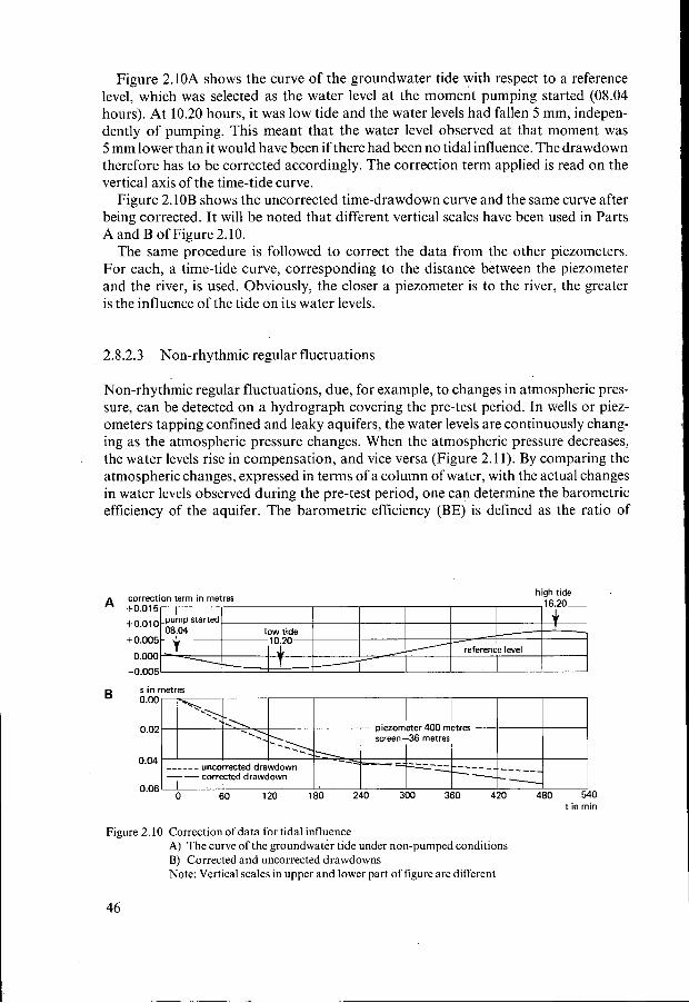
Figure 2.10A shows the curve of the groundwater tide with respect to a reference level, which was selected as the water level at the moment pumping started (08.04 hours). At 10.20 hours, it was low tide and the water levels had fallen 5 mm, indepen- dently of pumping. This meant that the water level observed at that moment was 5 mm lower than it would have been if there had been no tidal influence. The drawdown therefore has to be corrected accordingly. The correction term applied is read on the vertical axis of the time-tide curve.
Figure 2.10B shows the uncorrected time-drawdown curve and the same curve after being corrected. It will be noted that different vertical scales have been used in Parts A and B of Figure 2.10.
The same procedure is followed to correct the data from the other piezometers. For each, a time-tide curve, corresponding to the distance between the piezometer and the river, is used. Obviously, the closer a piezometer is to the river, the greater is the influence of the tide on its water levels.
. - '.
2.8.2.3 Non-rhythmic regular fluctuations
Y
---y., 0.02
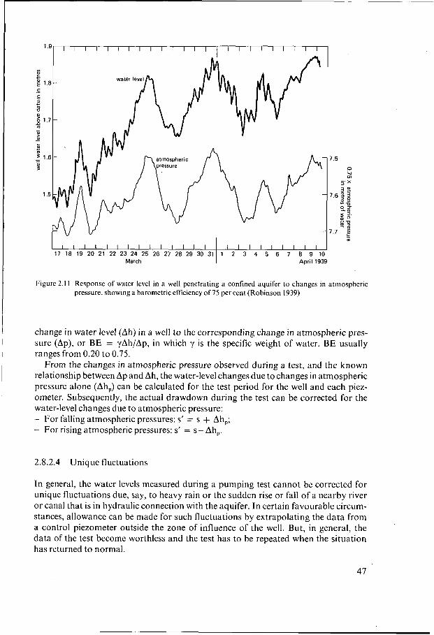
Non-rhythmic regular fluctuations, due, for example, to changes in atmospheric pres- sure, can be detected on a hydrograph covering the pre-test period. In wells or piez- ometers tapping confined and leaky aquifers, the water levels are continuously chang- ing as the atmospheric pressure changes. When the atmospheric pressure decreases, the water levels rise in compensation, and vice versa (Figure 2.1 1). By comparing the atmospheric changes, expressed in terms of a column of water, with the actual changes in water levels observed during the pre-test period, one can determine the barometric efficiency of the aquifer. The barometric efficiency (BE) is defined as the ratio of
piezometer 400 metres screen-36 metres -_ - -+,
high tide correction term in metres
A +0.015
f0.010
+ 0.005
0.000
-0.005
------ uncorrected drawdown 0.04
corrected drawdown -- I
B
--=-- '--y- _. - - - - - - - - - _ _ - - - 0.06 I
46
1.9 ~ 1 1 1 1 1 1 1 1 1 1 1 1 1 I I I I I I I I I
I I I I I I I I I I I I I I I I I I I I I I I 17 18 19 20 21 22 23 24 25 26 27 28 29 30 31 1 2 3 4 5 6 7 8 9 1(
March April 193
1
Figure 2. I I Response of water level in a well penetrating a confined aquifer to changes in atmospheric pressure, showing a barometric efficiency of 75 per cent (Robinson 1939)
change in water level (Ah) in a well to the corresponding change in atmospheric pres- sure (Ap), or BE = yAh/Ap, in which y is the specific weight of water. BE usually ranges from 0.20 to 0.75.
From the changes in atmospheric pressure observed during a test, and the known relationship between Ap and Ah, the water-level changes due to changes in atmospheric pressure alone (Ah,,) can be calculated for the test period for the well and each piez- ometer. Subsequently, the actual drawdown during the test can be corrected for the water-level changes due to atmospheric pressure: - For falling atmospheric pressures: s’ = s + Ah,,; - For rising atmospheric pressures: s’ = s - Ahp.
2.8.2.4 Unique fluctuations
In general, the water levels measured during a pumping test cannot be corrected for unique fluctuations due, say, to heavy rain or the sudden rise or fall of a nearby river or canal that is in hydraulic connection with the aquifer. In certain favourable circum- stances, allowance can be made for such fluctuations by extrapolating the data from a control piezometer outside the zone of influence of the well. But, in general, the data of the test become worthless and the test has to be repeated when the situation has returned to normal.
47
2.9 Interpretation of the data
Calculating hydraulic characteristics would be relatively easy if the aquifer system (i.e. aquifer plus well) were precisely known. This is generally not the case, so interpret- ing a pumping test is primarily a matter of identifying an unknown system. System identification relies on models, the characteristics of which are assumed to represent the characteristics of the real aquifer system.
Theoretical models comprise the type of aquifer (Section 1.2), and initial and bound- ary conditions. Typical outer boundary conditions were mentioned in Section 1.4. Inner boundary conditions are associated with the pumped well (e.g. fully or partially penetrating, small or large diameter, well losses).
In a pumping test, the type of aquifer and the inner and outer boundary conditions dominate at different times during the test. They affect the drawdown behaviour of the system in their own individual ways. So, to identify an aquifer system, one must compare its drawdown behaviour with that of the various theoretical models. The model that compares best with the real system is then selected for the calculation of the hydraulic characteristics.
System identification includes the construction of diagnostic plots and specialized plots. Diagnostic plots are log-log plots of the drawdown versus the time since pump- ing started. Specialized plots are semi-log plots of drawdown versus time, or drawdown versus distance to the well; they are specific to a given flow regime. A diagnostic plot allows the dominating flow regimes to be identified; these yield straight lines on special- ized plots. The characteristic shapes of the curves can help in selecting the appropriate model.
In a number of cases, a semi-log plot of drawdown versus time has more diagnostic value than a log-log plot. We therefore recommend that both types of graphs be con- structed.
The choice of theoretical model is a crucial step in the interpretation of pumping tests. If the wrong model is chosen, the hydraulic characteristics calculated for the real aquifer will not be correct. A troublesome fact is that theoretical solutions to well-flow problems are usually not unique. Some models, developed for different aquifer systems, yield similar responses to a given stress exerted on them. This makes system identification and model selection a difficult affair. One can reduce the number of alternatives by conducting more field work, but that could make the total costs of the test prohibitive. In many cases, uncertainty as to which model to select will remain. We shall discuss this problem briefly below. The examples we give will illus- trate that analyzing a pumping test is not merely a matter of opening a particular page of this book and applying the method described there.
2.9.1 Aquifer categories
Aquifers fall into two broad categories: unconsolidated aquifers and consolidated frac- tured aquifers. Within both categories, the aquifers may be confined, unconfined, or leaky (Section 1.2, Figure 1.1). We shall first consider all three types of unconsolidated aquifer, and then the consolidated aquifer, but only the confined type.
Figure 2.12 shows log-log and semi-log plots of the theoretical time-drawdown rela-
48
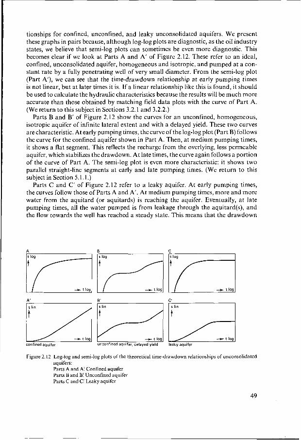
tionships for confined, unconfined, and leaky unconsolidated aquifers. We present these graphs in pairs because, although log-log plots are diagnostic, as the oil industry states, we believe that semi-log plots can sometimes be even more diagnostic. This becomes clear if we look at Parts A and A’ of Figure 2.12. These refer to an ideal, confined, unconsolidated aquifer, homogeneous and isotropic, and pumped at a con- stant rate by a fully penetrating well of very small diameter. From the semi-log plot (Part A’), we can see that the time-drawdown relationship at early pumping times is not linear, but at later times it is. If a linear relationship like this is found, it should be used to calculate the hydraulic characteristics because the results will be much more accurate than those obtained by matching field data plots with the curve of Part A. (We return to this subject in Sections 3.2.1 and 3.2.2.)
Parts B and B’ of Figure 2.12 show the curves for an unconfined, homogeneous, isotropic aquifer of infinite lateral extent and with a delayed yield. These two curves are characteristic. At early pumping times, the curve of the log-log plot (Part B) follows the curve for the confined aquifer shown in Part A. Then, at medium pumping times, it shows a flat segment. This reflects the recharge from the overlying, less permeable aquifer, which stabilizes the drawdown. At late times, the curve again follows a portion of the curve of Part A. The semi-log plot is even more characteristic: it shows two parallel straight-line segments at early and late pumping times. (We return to this subject in Section 5.1.1 .)
Parts C and C’ of Figure 2.12 refer to a leaky aquifer. At early pumping times, the curves follow those of Parts A and A’. At medium pumping times, more and more water from the aquitard (or aquitards) is reaching the aquifer. Eventually, at late pumping times, all the water pumped is from leakage through the aquitard(s), and the flow towards the well has reached a steady state. This means that the drawdown
A E’ I s lin
E Í unconfined aquifer, delayed + yield t log
C‘ s lin
Figure 2.12 Log-log and semi-log plots of the theoretical time-drawdown relationships of unconsolidated aquifers: Parts A and Ai Confined aquifer Parts B and Bi Unconfined aquifer Parts C and Ci Leaky aquifer
49
in the aquifer stabilizes, as is clearly reflected in both graphs. (We return to this subject in Sections 4.1.1 and 4.1.2.)
We shall now consider the category of confined, consolidated fractured aquifers, some examples of which are shown in Figure 2.13. Parts A and A’ of this figure refcr to a confined, densely fractured, consolidated aquifer of the double-porosity type. In an aquifer like this, we recognize two systems: the fractures of high permeability and low storage capacity, and the matrix blocks of low permeability and high storage capacity. The flow towards the well in such a system is entirely through the fractures and is radial and in an unsteady state. The flow from the matrix blocks into the frac- tures is assumed to be in a pseudo-steady state. Characteristic of the flow in such a system is that three time periods can be recognized: - Early pumping time, when all the flow comes from storage in the fractures; - Medium pumping time, a transition period during which the matrix blocks feed
their water at an increasing rate to the fractures, resulting in a (partly) stabilizing drawdown;
- Late pumping time, when the pumped water comes from storage in both the frac- tures and the matrix blocks.
(We return to this subject in Chapter 17.) The shapes of the curves in Parts A and A‘ of Figure 2.13 resemble those of Parts
B and B’ of Figure 2.12, which refer to an unconfined, unconsolidated aquifer with delayed yield.
Parts B and B’ of Figure 2.13 present the curves for a well that pumps a single plane vertical fracture in a confined, homogeneous, and isotropic aquifer of low perme- ability. The fracture has a finite length and a high hydraulic conductivity. Characteris- tic of this system is that a log-log plot of early pumping time shows a straight-line segment of slope 0.5. This segment reflects the dominant flow regime in that period:
Figure 2.13 Log-log and semi-log plots of the theoretical time-drawdown relationships of consolidated,
pumped well in single plane,
fractured aquifers: Parts A and A‘: Confined fractured aquifer, double porosity type Parts Band B’: A single plane vertical fracture Parts C and C’: A permeable dike in an otherwise poorly permeable aquifer
50
it is horizontal, parallel, and perpendicular to the fracture. This flow regime gradually changes, until, at late time, it becomes pseudo-radial. The shapes of the curves at late time resemble those of Parts A and A' of Figure 2.12. (We return to this subject in Section 18.3.)
Parts C and C' of Figure 2.1 3 refer to a well in a densely fractured, highly permeable dike of infinite length and finite width in an otherwise confined, homogeneous, isotro- pic, consolidated aquifer of low hydraulic conductivity and high storage capacity. Characteristic of such a system are the two straight-line segments in a log-log plot of early and medium pumping times. The first segment has a slope of 0.5 and thus resembles that of the well in the single, vertical, plane fracture shown in Part B of Figure 2.13. At early time, the flow towards the well is exclusively through the dike, and this flow is parallel. At medium time, the adjacent aquifer starts yielding water to the dike. The dominant flow regime in the aquifer is then near-parallel to parallel, but oblique to the dike. In a log-log plot, this flow regime is reflected by a one-fourth slope straight-line segment. At late time, the dominant flow regime is pseudo-radial, which, in a semi-log plot, is reflected by a straight line.
The one-fourth slope straight-line segment does not always appear in a log-log plot; whether it does or not depends on the hydraulic diffusity ratio between the dike and the adjacent aquifer. (We return to this subject in Section 19.3.)
2.9.2 Specific boundary conditions
When field data curves of drawdown versus time deviate from the theoretical curves of the main types of aquifer, the deviation is usually due to specific boundary condi- tions (e.g. partial penetration of the well, well-bore storage, recharge boundaries, or impermeable boundaries). Specific boundary conditions can occur individually (e.g. a partially penetrating well in an otherwise homogeneous, isotropic aquifer of infinite extent), but they often occur in combination (e.g. a partially penetrating well near a deeply incised river or canal). Obviously, specific boundary conditions can occur in all types of aquifers, but the examples we give below refer only to unconsolidated, confined aquifers.
Purtialpenetrution of the well Theoretical models usually assume that the pumped well fully penetrates the aquifer, so that the flow towards the well is horizontal. With a partially penetrating well, the condition of horizontal flow is not satisfied, at least not in the vicinity of the well. Vertical flow components are thus induced in the aquifer, and these are accompanied by extra head losses in and near the well. Figure 2.14 shows the effect of partial penet- ration. The extra head losses it induces are clearly reflected. (We return to this subject in Chapter IO.)
Well-bore storage All theoretical models assume a line source or sink, which means that well-bore storage effects can be neglected. But all wells have a certain dimension and thus store some water, which must first be removed when pumping begins. The larger the diameter of the well, the more water it will store, and the less the condition of line source or
51
A I
Figure 2.14 The effect of the well’s partial penetration on the time-drawdown relationship in an unconsoli- dated, confined aquifer. The dashed curves are those of Parts A and A of Figure 2.12
sink will be satisfied. Obviously, the effects of well-bore storage will appear at early pumping times, and may last from a few minutes to many minutes, depending on the storage capacity of the well. In a log-log plot of drawdown versus time, the effect of well-bore storage is reflected by a straight-line segment with a slope of unity. (We return to this subject in Section 15.1.1 .)
If a pumping test is conducted in a large-diameter well and drawdown data from
that those data will also be affected by the well-bore storage in the pumped well. At early pumping time, the data will deviate from the theoretical curve, although, in a log-log plot, no early-time straight-line segment of slope unity will appear. Figure 2.15 shows the effect of well-bore storage on time-drawdown plots of observation wells or piezometers. (We return to this subject in Section 1 1.1 .)
I I
observation wells or piezometers are used in the analysis, it should not be forgotten 1
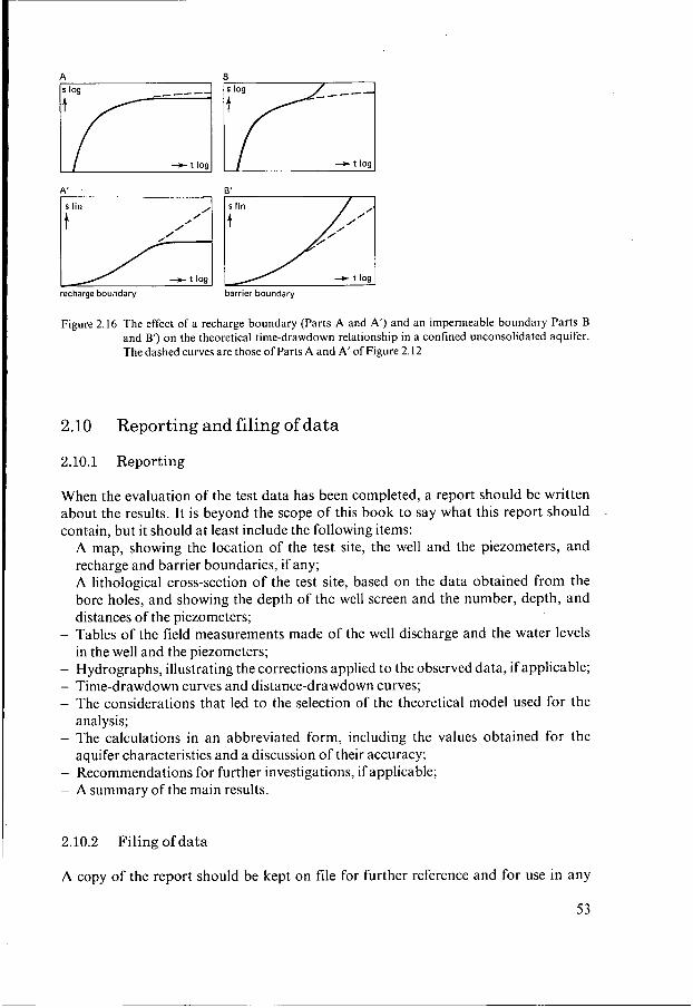
Recharge or impermeable boundaries The theoretical curves of all the main aquifer types can also be affected by recharge or impermeable boundaries. This effect is shown in Figure 2.16. Parts A and A of that figure show a situation where the cone of depression reaches a recharge boundary. When this happens, the drawdown in the well stabilizes. The field data curve then begins to deviate more and more from the theoretical curve, which is shown in the dashed segment of the curve. Impermeable (no-flow) boundaries have the opposite effect on the drawdown. If the cone of depression reaches such a boundary, the draw- down will double. The field data curve will then steepen, deviating upward from the theoretical curve. This is shown in Parts B and B’ of Figure 2.16. (We return to this subject in Chapter 6.)
well.bore storage
Figure 2.15 The effect of well-bore storage in the pumped well on the theoretical time-drawdown plots of observation wells or piezometers. The dashed curves are those of Parts A and A’ of Figure 2.12
52
recharge boundary barrier boundary
Figure 2.16 The effect of a recharge boundary (Parts A and A’) and an impermeable boundary Parts B and B’) on the theoretical time-drawdown relationship in a confined unconsolidated aquifer. The dashed curves are those of Parts A and A’ of Figure 2.12
2.10 Reporting and filing of data
2.10.1 Reporting
When the evaluation of the test data has been completed, a report should be written about the results. It is beyond the scope of this book to say what this report should contain, but it should at least include the following items: - A map, showing the location of the test site, the well and the piezometers, and
recharge and barrier boundaries, if any; - A lithological cross-section of the test site, based on the data obtained from the
bore holes, and showing the depth of the well screen and the number, depth, and distances of the piezometers;
- Tables of the field measurements made of the well discharge and the water levels in the well and the piezometers;
- Hydrographs, illustrating the corrections applied to the observed data, if applicable; - Time-drawdown curves and distance-drawdown curves; - The considerations that led to the selection of the theoretical model used for the
analysis; - The calculations in an abbreviated form, including the values obtained for the
aquifer characteristics and a discussion of their accuracy; - Recommendations for further investigations, if applicable; - A summary of the main results.
2.10.2 Filing of data
A copy of the report should be kept on file for further reference and for use in any
53
later studies. Samples of the different layers penetrated by the borings should also be filed, as should the basic field measurements of the pumping test. The conclusions drawn from the test may become obsolete in the light of new insights, but the hard facts, carefully collected in the field, remain facts and can always be re-evaluated.