Lima Vehicle Activity Study Conducted December 01 - 12, 2003 Final Report Submitted June 28, 2004 James Lents, [email protected]Nicole Davis, [email protected]International Sustainable Systems Research (http://www.issrc.org ) 21573 Ambushers St., Diamond Bar, CA 91765, USA Nick Nikkila, [email protected]Global Sustainable Systems Research (http://www.gssr.net/ ) 7146 Aloe Court, Rancho Cucamonga, CA 91739, USA Mauricio Osses, [email protected]University of Chile (http://www.uchile.cl ) Department of Mechanical Engineering, Casilla 2777, Santiago, Chile
Transcript
Lima Vehicle Activity Study
Conducted December 01 - 12, 2003 Final Report Submitted June 28, 2004
I. INTRODUCTION..............................................................................................................................................1 II. VEHICLE TECHNOLOGY DISTRIBUTION...............................................................................................3
II.A. BACKGROUND AND OBJECTIVES .................................................................................................................3 II.B. METHODOLOGY...........................................................................................................................................3 II.C. SURVEY RESULTS........................................................................................................................................7
IV. VEHICLE START PATTERNS................................................................................................................27 IV.A. BACGROUND AND OBJECTIVES ..................................................................................................................27 IV.B. METHODOLOGY.........................................................................................................................................27 IV.C. RESULTS ....................................................................................................................................................27
V. IVE APPLICATION AND EMISSIONS RESULTS....................................................................................29 APPENDIX A DATA COLLECTION PROGRAM USED IN LIMA .................................................................................A.1 APPENDIX B DAILY LOG OF THE DATA COLLECTION PROGRAM CONDUCTED IN LIMA...........................B.1
iii
1
EXECUTIVE SUMMARY Lima, Peru was visited from December 1, 2003 to December 15, 2003 to collect and analyze data related to on-road transportation. The study effort was designed to support estimates of the air pollution impacts of on-road transportation in Lima that will be used in the development of air quality management plans for the region. It is also hoped that the collected data can be extrapolated to other Peruvian cities to support environmental improvement efforts in the other cities as well. The data collection effort was a partnership between Lima local and regional governments, Universidad Nacional Mayor de San Marcos (UNMSM)
1
, non-government officials, and the International Sustainable Systems Research Center (ISSRC) in cooperation with the University of California at Riverside (UCR). The Clean Air Initiative in Latin American Cities provided technical and financial support. In all, about thirty persons participated in data collection activities over an approximate two week period. The study collected three types of information on vehicles operating on Lima streets: technology distribution, driving patterns, and start patterns. Each area is summarized below. Vehicle Technology Distribution
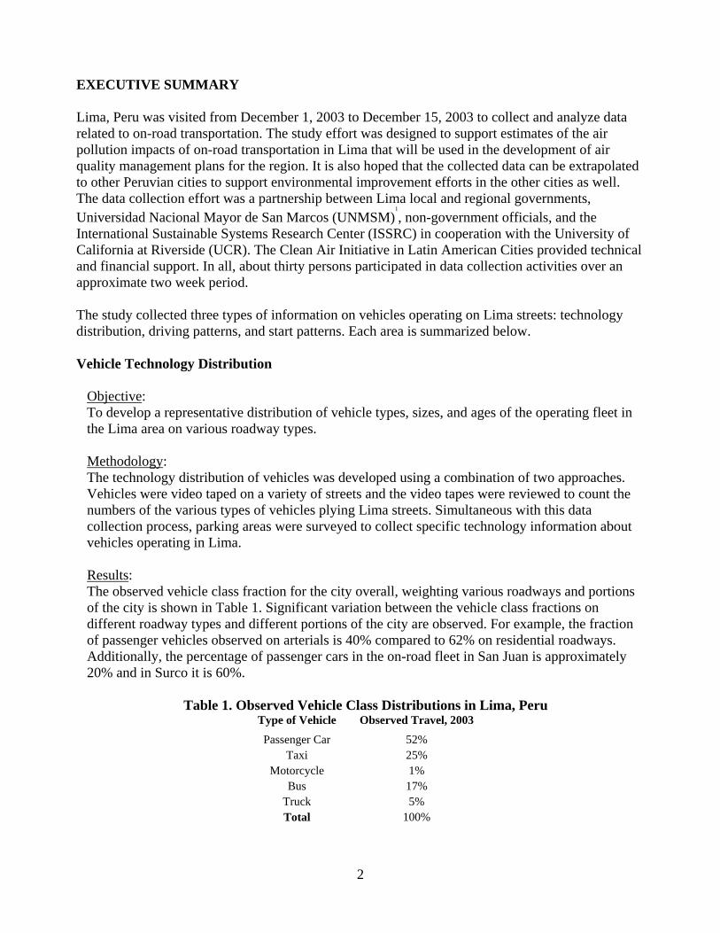
Objective: To develop a representative distribution of vehicle types, sizes, and ages of the operating fleet in the Lima area on various roadway types. Methodology: The technology distribution of vehicles was developed using a combination of two approaches. Vehicles were video taped on a variety of streets and the video tapes were reviewed to count the numbers of the various types of vehicles plying Lima streets. Simultaneous with this data collection process, parking areas were surveyed to collect specific technology information about vehicles operating in Lima. Results: The observed vehicle class fraction for the city overall, weighting various roadways and portions of the city is shown in Table 1. Significant variation between the vehicle class fractions on different roadway types and different portions of the city are observed. For example, the fraction of passenger vehicles observed on arterials is 40% compared to 62% on residential roadways. Additionally, the percentage of passenger cars in the on-road fleet in San Juan is approximately 20% and in Surco it is 60%.
Table 1. Observed Vehicle Class Distributions in Lima, Peru
Type of Vehicle Observed Travel, 2003
Passenger Car 52% Taxi 25%
Motorcycle 1% Bus 17%
Truck 5% Total 100%
2
In addition to observing the class distribution, a separate survey was conducted to determine the emissions control technology and engine type of the passenger fleet. Over half of the passenger vehicles have no catalyst, and approximately 40% have three way catalysts. The majority of passenger vehicles on the road are gasoline carbureted vehicles.
Vehicle Driving Patterns
Objectives: To collect second-by-second information on the speed and acceleration of the main types of vehicles operating in Lima on a representative set of roadways throughout the day. Methodology: The driving patterns for the various classes of vehicles were measured using Global Positioning Satellite (GPS) technology. This technology allows for the second by second measurements of vehicle speeds and altitude. GPS units were carried on nine selected routes. Data was collected from 07:00 to 19:00 to provide driving pattern information for differing times of the day. Results: Driving pattern data was successfully collected over 6 days from a number of passenger vehicles, taxis, buses and delivery trucks. Overall, various road types and vehicle types have similar average velocities. It is interesting that the fastest and lowest velocities occur on the highways, the highest speeds during the very early morning hours and lowest velocities in the middle of the day, when average speeds are even lower than on residential roadways. Delivery trucks maintain a relatively low average velocity throughout the day due to the idle time during deliveries. Buses and taxis have similar average speeds to passenger vehicles traveling on arterial and residential roadways. Taxis and passenger vehicles operating on the highway during the middle of the day and evening exhibit the highest occurrences of hard accelerations, due to congestion and high target velocities.
Vehicle Start Patterns
Objective: To collect a representative sample of the number, time of day, and soak period from passenger vehicles operating in Lima. Methodology: The vehicle engine start patterns were collected using equipment that senses vehicle system voltage denoted VOCE units. VOCE data can be used to determine when vehicles start, how long they operate, and how long they sit idle between starts. This information is essential to establish vehicle start emissions. The VOCE units were placed in passenger vehicles and left there for a period of a week. Results: Over 340 days of start patterns from 80 different vehicles were collected over the study period. The results show that on average, a typical passenger car is started 5.6 times per day. Approximately 20% of the starts occur between 6 am and 9 am, and another 20% occur between 3 pm and 6 pm. In the early morning hours, over half of the starts occur after having soaked over 12 hours. These long soaks leave the engine cold, which results in increased starting emissions.
3
Conclusions
The three types of data collected in this study have been used to compile a comprehensive analysis of the make-up and behavior of the current on-road mobile fleet in Lima. This data is pertinent for correctly estimating current mobile source emissions and projecting the impact of proposed control strategies and growth scenarios, because the vehicle type, speed profiles, and the number of starts and the soak period have a large impact on the mobile source emissions inventory. The data collected in this study was formatted to allow vehicle emissions estimates using the International Vehicle Emissions Model (http://www.issrc.org/ive or www.gssr.net/ive). The IVE model was developed with USEPA funding to make emissions estimates under different technology and driving situations as found in various countries, and has been used extensively in several developing countries. Although up-to date vehicles activity and fleet information was collected in this study, no emissions measurements were made. All emission estimates conducted using the IVE model’s default emission rates. It is recommended that some emission measurements be conducted to create Lima specific emissions. Overall, the results of this study have shown that driving in Lima is similar to other developing urban areas with some subtle but important differences. The number of starts per day and the kilometers driven per day per passenger vehicle is slightly lower than seen in other areas researched to date. Of all the areas observed to date, Lima has the lowest percentage of passenger vehicles (including two-wheeled vehicles as passenger vehicles) and the highest percentage of small buses and trucks. The average age of the passenger fleet and average mileage accumulation varies widely from city to city in the countries studied to date, but Lima falls in the middle of this range for both variables. Lima’s passenger fleet is comprised of approximately half non catalyst vehicles, compared to 1% in the US; 20-30% in Mexico City, Santiago, and Pune; and 90-100% in Almaty and Nairobi. A preliminary emissions analysis using the IVE model indicate that on the order of 22 metric tons of PM, 370 tons of NOx, 200 tons of VOC, and 3,500 tons/day of CO are emitted from on-road motor vehicles each day in Lima. By viewing the contribution of various vehicle types to the inventory, it was determined that to reduce PM (and toxic) emissions in Lima, buses and trucks must be controlled. To reduce NOx, buses, trucks, and passenger vehicles must be further controlled. All of these types of vehicles in the Lima fleet have better emissions control alternatives that could be employed to reduce emissions. Lima currently has the second highest emission rate for PM and NOx on a per vehicle mile basis from the urban areas in Los Angeles, Nairobi, Santiago, Pune and Mexico City, largely due to the lack of control technology on the trucks, buses, and passenger vehicles operating in the area, and the fact that a higher percentage of the fleet is trucks and buses. It must be noted again that the emissions analysis is subject to the appropriateness of the emission rates used in the IVE model. Several recommendations for additional study include using the tools outlined in this report to develop a strategy for improving future air quality, determine the appropriateness of the collected data to suburban areas outside of Lima or other urban areas within Peru, and improve the emission factors for in-use vehicles. An improved estimate of current overall vehicular travel (VKT) and future growth rates is also recommended.
I. INTRODUCTION The vehicle activity study was conducted in Lima, Peru, was from December 1, 2003 to December 15, 2003. During this time, in cooperation with local universities and government officials, three types of information were collected. Subsequently, this data was processed and analyzed and put into a format to be used in the IVE model. The data, collection process, comparisons with other areas studied, and emissions results from the IVE modeled are reported in this paper. The data collected has three purposes:
• To estimate the technology distribution of vehicles operating on Lima streets. • To measure driving patterns for the various classes of vehicles operating on Lima streets. • To estimate the times and numbers of vehicle engine starts for the various classes of vehicles
operating on Lima streets. The technology distribution of vehicles was developed using a combination of two approaches. Vehicles were video taped on a variety of streets and the video tapes were reviewed to count the numbers of the various types of vehicles plying Lima streets. Simultaneous with this data collection process, parking areas were surveyed to collect specific technology information about vehicles operating in Lima. The driving patterns for the various classes of vehicles were measured using Global Positioning Satellite (GPS) technology. This technology allows for the second by second measurements of vehicle speeds. GPS units were carried on a variety of vehicles on a variety of street types throughout the metropolitan area. Data was collected from 07:00 to 19:00 to provide driving pattern information for differing times of the day. The vehicle engine start patterns were collected using equipment that senses vehicle system voltage denoted VOCE units. VOCE data can be used to determine when vehicles start, how long they operate, and how long they sit idle between starts. This information is essential to establish vehicle start emissions. The data collected in this study was formatted to allow vehicle emissions estimates using the International Vehicle Emissions Model (http://www.issrc.org/ive or www.gssr.net/ive). This model was developed with USEPA funding to make emissions estimates under different technology and driving situations as found in various countries. Each process and results are described in detail in the next sections.
II. VEHICLE TECHNOLOGY DISTRIBUTION II.A. BACKGROUND AND OBJECTIVES The most critical element of on-road transportation emissions analysis is the nature of the vehicle technologies that operate on the street or in the region of interest. Differing vehicle technologies can produce considerably different rates of emissions. Vehicles operating on the same roads can produce emissions that are 300 times different from one another. The fractions of various types of vehicles in a local fleet and the fractions of these various types of vehicles actually operating on the roadways are not necessarily the same. This difference occurs because some classes of vehicles are operated considerably more than other classes vehicles. For example, a class of vehicles that operates twice as much as another class will produce an on-road fraction that is twice as great even if there are equal numbers of vehicles in the static fleet. The fraction of interest for estimating on-road emissions is the fraction of driving contributed by the various vehicle technologies since this will correspond to the about of air emissions that are produced. Thus, the most accurate estimate of vehicular contribution to air emissions is made by determining the fractions of the various vehicle technology classes actually operating on city streets rather than the distribution of vehicles registered in the region of interest. The objective of this portion of the study is to develop a representative distribution of vehicle types, sizes, and ages of the operating fleet in the Lima area on various roadway types through a passenger survey. The goal of the survey was to identify the specific engine technologies, drive train, control technologies, air conditioning, total use, and model years of the vehicles surveyed. II.B. METHODOLOGY In order to insure that the most representative data is collected, both video-traffic and parked vehicle studies were carried out from 07:00 in the morning to 19:00 in the evening over 6 days in 3 representative sections of the urban area. Surveys were carried out on or near (in the cases of parked vehicle surveys) a residential street, an arterial roadway, and a highway in each area surveyed. Figure II.1 shows the three different areas where both parking lot and video taping activities were carried out.
3
Sector A: Surco
Sector B: San Juan Villamaria
Sector C: San Isidro
Figure II.1: Sectors where Activity Study was carried out in Lima, Peru To determine the fractions of the various vehicle technology classes operating on city streets, video cameras were set up along the sides of the road and traffic movement taped. Figure II.2 illustrates this process on a residential street in Lima, Peru.
Figure II.2: Video Taping Road Traffic in Lima, Peru
4
The completed videotapes were analyzed in slow motion to insure the most accurate counts of vehicles, as it is shown in Figure II.3.
Figure II.3: Video Tape Counting at UNMSM, Lima, Peru
It is not possible using the video taping process to determine the exact nature of the vehicle technologies observed. The video taping allowed the determination of the fractions of trucks, buses, passenger vehicles, 2-wheelers, and such operating on the roadways of interest. To understand the specific technologies of local vehicles, parking surveys were completed. Parked vehicle surveys allow careful inspection of vehicles so that the engine technology, model year, control equipment, and fuel type can be established. The parked vehicle surveys were used to estimate the more specific natures of the general vehicle classifications determined from the video tape studies. The parking lot survey in Lima was directed by Cesar Ramirez of the Servicio Nacional de Adiestramiento en Trabajo Industrial (SENATI). Two teams of students were used in the study. One team was experienced with respect to vehicle technologies and the other group was experienced with respect to survey methodologies. The two teams worked the same areas each day following the schedule and locations selected for video tape recordings (Table II.1). Figure II.4 illustrates the training process for the students at UNMSM, and Figure II.5 shows the actual parking lot survey process in Lima, Peru.
Figure II.4: Training for students participating in the Parking Lot Survey
5
Figure II.5: Parking Lot Survey in Lima, Peru
Table II.1 indicates the locations in Lima where video surveys were completed. These locations were suggested by the Lima city officials as representative of the general metropolitan area. They also represent the locations were driving patterns were measured. Parking surveys were completed at locations generally in the vicinity of the video surveys.
Table II.1 Video Locations Surveyed in Lima, Peru Street Type Location Date and Hour of Surveys
Wed, Dec 3 @ 09:00, 12:00 Highway A1 Av. Javier Prado - Surco Fri, Dec 5 @ 13:00, 16:00, 19:00 Thu, Dec 4 @ 06:00, 11:00 Highway B1 Av. Panamericana Sur - San Juan Wed, Dec 10 @ 15:00, 18:00 Tue, Dec 9 @ 07:00, 10:00 Highway C1 Av. Paseo de la Republica - San Isidro Thu, Dec 11 @ 14:00, 17:00 Wed, Dec 3 @ 07:00, 10:00 Arterial A2 Av. Las Palmeras - Surco Fri, Dec 5 @ 14:00, 17:00 Thu, Dec 4 @ 07:00, 09:00 Arterial B2 Av. Los Héroes - San Juan Wed, Dec 10 @ 13:00, 16:00 Tue, Dec 9 @ 08:00, 11:00 Arterial C2 Av. Arequipa - San Isidro Thu, Dec 11 @ 15:00, 18:00 Wed, Dec 3 @ 08:00, 11:00 Residential A3 Av. Via Lactea - Surco Fri, Dec 5 @ 15:00, 18:00
Thu, Dec 4 @ 10:00 Residential B3 J. C. Tello - San Juan Wed, Dec 10 @ 14:00, 17:00 Tue, Dec 9 @ 06:00, 09:00, 12:00 Residential C3 Av. Conquistadores - San Isidro Thu, Dec 11 @ 13:00, 19:00
6
Two cameras were placed along roads as described in Table II.1. The cameras were operated for 20 minutes during the hour of interest. The cameras were then moved to the next location of interest and again operated for 20 minutes. The 20 minute operation times were selected to yield a significant amount of data and to allow for disassembly movement to a new location and reassembly in order to collect data in the next hour. The actual 20 minutes surveyed in any hour was random depending upon the time it took to move the cameras from one location and get them set up in a second location. The schedules followed are shown in the preceding Table II.1. The video tapes were reviewed in slow motion and stop action as needed to yield accurate analysis of the roadway vehicle distributions. This is a key advantage of using video tape instead of direct human observation. There was a misunderstanding in the data collection schedule such that in a few cases the video camera operators failed to collect data on certain hours. Information for these few hours was estimated using adjacent hours. Also, video counts from individual vehicle categories varied considerably from hour to hour due to the limited video taping time. To correct for this, we used the overall vehicle flow, which was more consistent, and then used the average vehicle category fractions to estimate typical vehicle flow for each vehicle category. II.C. SURVEY RESULTS II.C.1. Fleet Composition Table II.2 below indicate the results of the analysis. As can be seen in Table II.2 the distribution of vehicles varies with street type and time of day. Thus, for highly time and street specific analysis, care must be taken to construct a proper technology distribution for the time and street of interest. For this analysis, overall average technology distributions are developed for the general metropolitan area.
Table II.2: Results of Analysis of Lima Videotapes Road type Area Time Vehicles
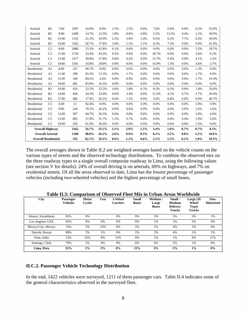
The overall averages shown in Table II.2 are weighted averages based on the vehicle counts on the various types of streets and the observed technology distributions. To combine the observed mix on the three roadway types to a single overall composite roadway in Lima, using the following values (see section V for details): 24% of overall driving is on arterials, 69% on highways, and 7% on residential streets. Of all the areas observed to date, Lima has the lowest percentage of passenger vehicles (including two-wheeled vehicles) and the highest percentage of small buses.
Table II.3: Comparison of Observed Fleet Mix in Urban Areas Worldwide City Passenger
II.C.2. Passenger Vehicle Technology Distribution In the end, 1422 vehicles were surveyed, 1211 of them passenger cars. Table II.4 indicates some of the general characteristics observed in the surveyed fleet.
8
Table II.4: General characteristics of the surveyed Passenger Cars Type of Fuel* Air Conditioning System Type of Transmission Catalytic Converter (CC) 72% Gasoline 71% with A/C 74% Mechanic Trans. 58% without CC 26% Diesel 29% without A/C 26% Automatic Trans. 42% with CC
• 2% LPG and gasoline (dual engines) The IVE Model defines 1328 technology classifications based on fuel type, engine technology, and control technology plus 45 user defined technologies. An example of six technology types for gasoline passenger vehicles is shown in Figure II.5:
Table II.5: IVE technology fractions of the Gasoline Passenger Cars
The engine size of the Lima vehicle fleet was generally midsize (1301-2000cc). Table II.6 indicates the engine size and use distribution of the passenger vehicle.
Table II.6: Size and Use Characteristics of the Surveyed Passenger Car Fleet Vehicle Engine Size 35% Low Use
(<80 K km) 32% Medium Use
(80-161 K km) 33% High Use (>161 K km)
17% Small (<1301 cc) 4.66% 6.81% 5.86% 74% Medium (1301-2000 cc) 25.83% 21.70% 25.98%
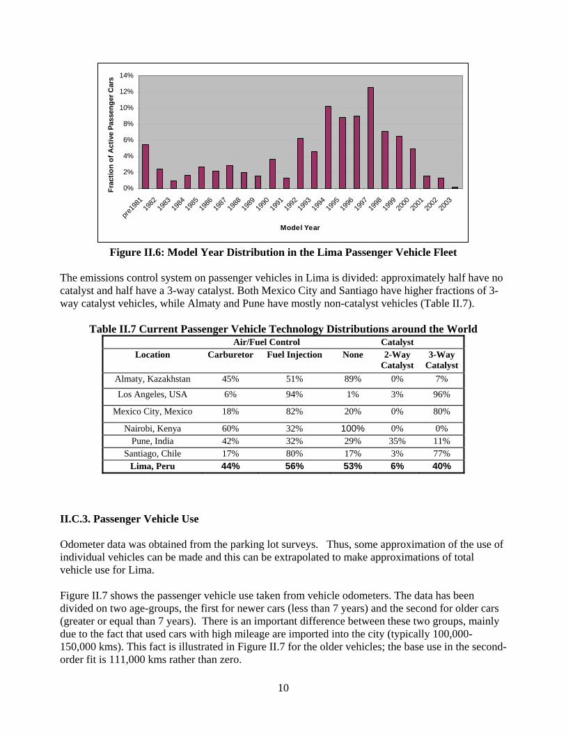
9% Large (>2000 cc) 4.28% 3.03% 1.85% Information in Table II.5 must be combined with information in Tables II.6 along with the video collected data in Table II.2 to produce the passenger vehicle information for estimating emissions. Figure II.6 illustrates the model year distribution for active passenger vehicles in Lima. The average age of passenger vehicles surveyed during the parking lot activity was 10.98 years. According to governmental registration figures (Parque Automotor Lima, Diciembre 2002, Dirección General de Circulación Terrestre, OGPP-MTC) the average age of registered passenger cars in Lima reaches up to 14 years.
9
0%
2%
4%
6%
8%
10%
12%
14%
pre19
8119
8219
8319
8419
8519
8619
8719
8819
8919
9019
9119
9219
9319
9419
9519
9619
9719
9819
9920
0020
0120
0220
03
Model Year
Frac
tion
of A
ctiv
e Pa
ssen
ger C
ars
Figure II.6: Model Year Distribution in the Lima Passenger Vehicle Fleet
The emissions control system on passenger vehicles in Lima is divided: approximately half have no catalyst and half have a 3-way catalyst. Both Mexico City and Santiago have higher fractions of 3-way catalyst vehicles, while Almaty and Pune have mostly non-catalyst vehicles (Table II.7).
Table II.7 Current Passenger Vehicle Technology Distributions around the World Air/Fuel Control Catalyst
II.C.3. Passenger Vehicle Use Odometer data was obtained from the parking lot surveys. Thus, some approximation of the use of individual vehicles can be made and this can be extrapolated to make approximations of total vehicle use for Lima. Figure II.7 shows the passenger vehicle use taken from vehicle odometers. The data has been divided on two age-groups, the first for newer cars (less than 7 years) and the second for older cars (greater or equal than 7 years). There is an important difference between these two groups, mainly due to the fact that used cars with high mileage are imported into the city (typically 100,000-150,000 kms). This fact is illustrated in Figure II.7 for the older vehicles; the base use in the second-order fit is 111,000 kms rather than zero.
10
y = -996.88x2 + 20923x + 111098R2 = 0.1464
y = -482.11x2 + 20295xR2 = 0.9394
0
50000
100000
150000
200000
250000
0 2 4 6 8 10
Vehicle Age [yrs]
Odo
met
er [k
m]
12
Figure II.7: Passenger Vehicle Use during the first fifteen years of age
As is typical for the United States and all other countries studied so far, vehicle use decreases with vehicle age. Using the age distribution illustrated in previous Figure II.6, the average passenger car age in Lima is approximately 11 years. Considering this figure and from the data analysis for the newer age-group of cars in Lima, it is possible to estimate an overall average for Lima passenger cars equals to 15,000 km/year, thus, an average daily driving of 41 kilometers of driving per day over the year (assuming 365 days/year). The scatter in the data for the high use years is due to the small numbers of vehicles observed with higher ages and the fact that the odometers themselves become unreliable. The equation shown in Figure IIc.1 will produce unreasonable results if extrapolated beyond 15 years due to the uncertainty in the odometer readings for vehicles older than 7 years. It may be more appropriate to replace the second order term in the vehicle use equation with a value that is similar in a relative sense to those measured in other countries. The same analysis indicated in the above paragraph, made for the older age-group trendline, generates an average of 10,000 km/year, but this figure seems unreliable due to the uncertainty in odometer readings for this group. The current travel in Lima is estimated to be approximately 70,729,000 kilometers per day in the Lima Metropolitan Area1. This estimate is used in the IVE analysis to project emissions for the whole city. Table II.8 below provides the estimated total driving based on measurements made in this study.
1 This calculation is based on a total passenger car fleet of 647,000 vehicles driving 41 km/day, and 178,000 non-passenger vehicles driving 200 km/day (public transport and trucks). Fleet estimates are based on data provided by Ministerio de Transportes y Comunicaciones (MTC), Parque Automotor Lima 2002. Source: Dirección General de Circulación Terrestre, produced by OGPP - Dirección de Información de Gestión Estadística.
11
Table II.8: Observed Travel Distribution by vehicle type in Lima
Type of Vehicle Fraction of
Observed Travel, 2003
Estimated Travel (km/day)
Thousands Passenger Car 51.65% 24,600
Taxi 24.92% 1,190 Motorcycle 1.25% 9,409
Bus 17.45% 23,130 Truck 4.73% 12,400 Total 100.00% 70,729
The values shown in Table II.8 should only be treated as approximations, but they should be in the ballpark of the true total driving occurring in Lima in 2003. A final issue of interest is to compare Lima driving with other areas. Figure II.8 illustrates the total driving per vehicle for the countries studied to date. As can be seen, passenger cars are driven the most in the United States and the least in Pune, India. For the first 10 years of age, Lima has a similar mileage pattern for passenger vehicles to the driving observed in Los Angeles, USA. As mentioned earlier, the data becomes unreliable after 10-12 years due to the uncertainty on the odometer readings.
Figure II.8: Comparison of Passenger Vehicle Use in different cities
Figure II.9 illustrates the average age of the on-road vehicle fleet in different cities where the IVE methodology has been carried on.
12
4.7
6.4 6.5 6.6
10.98 11.3
13.2
0
2
4
6
8
10
12
14
16
Pune,
India
Mexico
City
, Mex
ico
Santia
go, C
hile
Los A
ngeles
, USA
Lima,
Peru
Almaty
, Kaz
akhs
tan
Nairob
i, Ken
ya
Aver
age
Age
[yrs
]
Figure II.9: Comparison of Average Vehicle Age in different cities
13
III. VEHICLE DRIVING PATTERNS III.A. BACKGROUND AND OBJECTIVES The main objective of this section is to collect second-by-second information on the speed and acceleration of the main types of vehicles operating in Lima on a representative set of roadways throughout the day. III.B. METHODOLOGY Vehicle driving patterns were measured using GPS technology as described in Appendix A. This technology allows the measurement each second of vehicle location, speed, and altitude. Three representative sections of the city were selected for the IVE study in Lima. The areas selected should represent a generally lower income area, a generally upper income area, and a commercial area of the city. Figure II.5 and Table III.1 show the sectors and streets selected in this study.
Table III.1 Streets selected for vehicle driving in Lima, Peru Street Type Location
Highway A1 Av. Javier Prado - Surco
Highway B1 Av. Panamericana Sur - San Juan
14
Highway C1 Av. Paseo de la Republica - San Isidro
Arterial A2 Av. Las Palmeras - Surco
Arterial B2 Av. Los Héroes - San Juan
Arterial C2 Av. Arequipa - San Isidro
Residential A3 Av. Via Lactea - Surco
15
Residential B3 J. C. Tello - San Juan
Residential C3 Av. Conquistadores - San Isidro
Figure III.1 illustrates the location data collected from one of the CGPS installed on a passenger car driving over Sector A in Lima. Roads A1 (Av. Javier Prado), A2 (Av. Panamericana Sur) and A3 (Av. Paseo de la República) can be identified with the drawings in Table III.1. III.C. RESULTS
-76.99
-76.985
-76.98
-76.975
-76.97
-76.965-12.095-12.09-12.085-12.08-12.075-12.07
Figure III.1: CGPS output from Sector A, Surco (streets A1, A2 and A3)
Figure III.2 presents an example of speeds as measured by the GPS unit for about 180 seconds around 11:30 driving a passenger car (Sector A, Surco).
Figure III.2: Example of Residential, Arterial, and Highway Driving at 11:30am in Lima Figure III.3 presents an example of altitude and velocity recorded from a small bus (Combi) over a 30 minutes drive. The altitude reading is the least certain of the data collected by a GPS unit, but it is still useful for estimating road grade.
Altitude Speed Figure III.3: Example of Altitude and Speed Recorded by GPS over a 30 Minutes Drive
In using this data to estimate road grade, care must be taken to look at multiple adjacent sample points to make the most appropriate estimate of road grade.
17
The IVE model uses a calculation of the power demand on the engine per unit vehicle mass to correct for the driving pattern impact on vehicle emissions. This power factor is called vehicle specific power (VSP). The VSP is the best, although imperfect, indicator of vehicle emissions relative the vehicles base emission rate. Equation III.1 presents the VSP equation used.
S = vehicle speed in km/second. dS/dt = vehicle acceleration km/second/second. Grade = grade of road grade radians.
About 65% of the variance in vehicle emissions can be accounted for using VSP. To further improve the emissions correction for vehicle driving, a factor denoted vehicle stress was developed. Vehicle stress (STR) uses an estimate of vehicle RPM combined with the average of the power exerted by the vehicle in the 15 seconds before the event of interest. Equation III.2 indicates the calculation for STR.
STR=RPM + 0.08*PreaveragePower III.2 Where,
RPM = the estimated engine RPM/1000 (an algorithm was developed by driving many different vehicles and measuring RPM compared to vehicle speed and acceleration. The minimum RPM allowed is 900. PreaveragePower = the average of VSP the 15 seconds before the time of interest. The 0.08 coefficient was developed from a statistical analysis of emissions and speed data from about 500 vehicles to give the best correction factor when combined with VSP.
Ultimately, the GPS data for each vehicle type studied is broken into one of 20 VSP bins and one of 3 STR Bins. Thus, each point along the driving route can be allocated to one of 60 driving bins. A given driving trace can be evaluated to indicate the fraction of driving that occurs in each driving bin. These fractions are used to develop a correction factor for a given driving situation. III.C.1. Passenger Cars Data on passenger car driving was collected in three parts of Lima (see Table II.1) over six days. Due to limited data, the driving data collected was allocated into 2 hour groups instead of 1 hour groups. Table III.2 indicates the average speed for each type of road studied for each 2-hour group.
Table III.2: Average Passenger Car Speeds on Lima Roads Time Highway Arterial Residential Street 5:30 51.82 24.58 21.63 7:30 51.82 24.58 21.63 9:30 38.15 24.84 21.80
Speed is not a good indicator of vehicle power demand. Vehicle acceleration consumes considerable energy and is not indicated by average vehicle speed. Tables III.3 to III.5 below provide the power bin distribution for the driving on Lima Highways, Arterials, and Residential streets respectively averaged over all hours. For use in the IVE model, the power bin distributions can also be used in the two hour groupings indicated in Table III.3 to make hourly estimates of emissions from passenger vehicles. It should be noted that Power Bins 1-11 represent the case of negative power (i.e. the vehicle is slowing down or going down a hill or some combination of each). Power Bin 12 represents the zero or very low power situation such as waiting at a signal light. Power Bins 13 and above represent the situation where the vehicle is using positive power (i.e. driving at a constant speed, accelerating, going up a hill or some combination of all three.
Table III.3: Distribution of driving into IVE Power Bins for passenger cars operating on Highways averaged over all hours (average speed: 37.49 km/hour)
Table III.4: Distribution of Driving into IVE Power Bins for Passenger Cars Operating on Arterials Averaged Over All Hours (average speed: 24.45 km/hour)
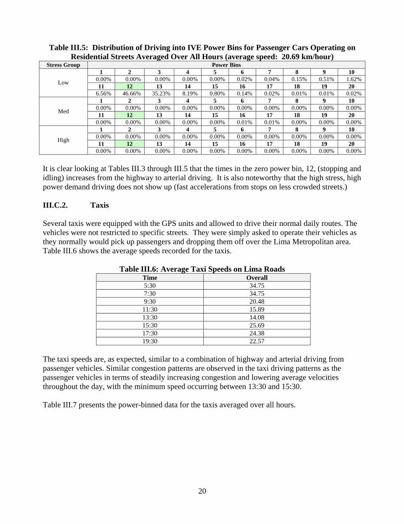
Table III.5: Distribution of Driving into IVE Power Bins for Passenger Cars Operating on Residential Streets Averaged Over All Hours (average speed: 20.69 km/hour)
0.00% 0.00% 0.00% 0.00% 0.00% 0.00% 0.00% 0.00% 0.00% 0.00% It is clear looking at Tables III.3 through III.5 that the times in the zero power bin, 12, (stopping and idling) increases from the highway to arterial driving. It is also noteworthy that the high stress, high power demand driving does not show up (fast accelerations from stops on less crowded streets.) III.C.2. Taxis Several taxis were equipped with the GPS units and allowed to drive their normal daily routes. The vehicles were not restricted to specific streets. They were simply asked to operate their vehicles as they normally would pick up passengers and dropping them off over the Lima Metropolitan area. Table III.6 shows the average speeds recorded for the taxis.
Table III.6: Average Taxi Speeds on Lima Roads Time Overall 5:30 34.75 7:30 34.75 9:30 20.48
The taxi speeds are, as expected, similar to a combination of highway and arterial driving from passenger vehicles. Similar congestion patterns are observed in the taxi driving patterns as the passenger vehicles in terms of steadily increasing congestion and lowering average velocities throughout the day, with the minimum speed occurring between 13:30 and 15:30. Table III.7 presents the power-binned data for the taxis averaged over all hours.
20
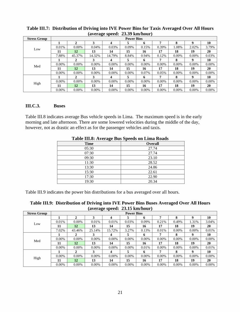
Table III.7: Distribution of Driving into IVE Power Bins for Taxis Averaged Over All Hours (average speed: 23.39 km/hour)
0.00% 0.00% 0.00% 0.00% 0.00% 0.00% 0.00% 0.00% 0.00% 0.00% III.C.3. Buses Table III.8 indicates average Bus vehicle speeds in Lima. The maximum speed is in the early morning and late afternoon. There are some lowered velocities during the middle of the day, however, not as drastic an effect as for the passenger vehicles and taxis.
Table III.8: Average Bus Speeds on Lima Roads Time Overall 05:30 27.74 07:30 27.74 09:30 23.10 11:30 28.52 13:30 24.86 15:30 22.61 17:30 22.90 19:30 20.34
Table III.9 indicates the power bin distributions for a bus averaged over all hours.
Table III.9: Distribution of Driving into IVE Power Bins Buses Averaged Over All Hours (average speed: 23.15 km/hour)
III.C.4. Trucks Table III.10 indicates average truck vehicle speeds in Lima. The maximum speed is in the early morning and evening. During the day the average velocity is significantly lower.
Table III.10: Average Delivery Truck Speeds on Lima Roads Time Overall 05:30 36.22 07:30 36.22 09:30 26.20 11:30 21.03 13:30 22.47 15:30 23.30 17:30 7.02 19:30 17.01
Table III.11 indicates the power bin distributions for the trucks averaged over all hours. A very large fraction of the truck driving pattern is spent idling. This idling is attributed to the deliveries the truck drivers make while the vehicle is still running. The daytime deliveries, in conjunction with daytime congestion, explain why the average velocity is so much lower during business hours, and lower than the buses. Table III.11: Distribution of Driving into IVE Power Bins Trucks Averaged Over All Hours
(average speed: 17.09 km/hour) Stress Group Power Bins
0.00% 0.00% 0.00% 0.00% 0.00% 0.00% 0.00% 0.00% 0.00% 0.00% III.C.5. Summary of Driving Pattern Results Figure III.4 compares driving speeds by hour for the four types of vehicles studied. In general, congestion lowers the average velocity during the daytime hours by 30 to 60 percent of free flow velocities. It was assumed that the early morning and late evening velocities were similar to the late evening and 6 AM data because no data was collected between 10 pm and 5 AM. Overall, various road types and vehicle types have similar average velocities. It is interesting that the fastest and lowest velocities occur on the highways, the highest speeds during the very early morning hours and lowest velocities in the middle of the day, when average speeds are even lower than on residential roadways. Delivery trucks maintain a relatively low average velocity throughout the day due to the idle time during deliveries. Buses and taxis have similar average speeds to passenger vehicles traveling on arterial and residential roadways.
22
0
10
20
30
40
50
60
0:00
1:00
2:00
3:00
4:00
5:00
6:00
7:00
8:00
9:00
10:00
11:00
12:00
13:00
14:00
15:00
16:00
17:00
18:00
19:00
20:00
21:00
22:00
23:00
Time of Day (hh:mm)
Aver
age
Vel
ocity
(kph
)
PCHwy PCRes PCArt 2wHwy 2wRes 2wArt Taxi Bus
Figure III.4: Average Speeds for All Road Types and Vehicle Classes in Lima
23
Figure III.5 shows the distribution into driving bins for four of the main classes of driving at 05:30. There is little to distinguish the driving patterns between passenger vehicles, 3-Wheel vehicles, and buses at this time of the morning. The 2-Wheel vehicles and passenger vehicles are using slightly more relative power (i.e. accelerations) in driving under free flow conditions.
Figure III.5: Comparison of Driving Patterns for Four Major Vehicle Classes for 05:30
24
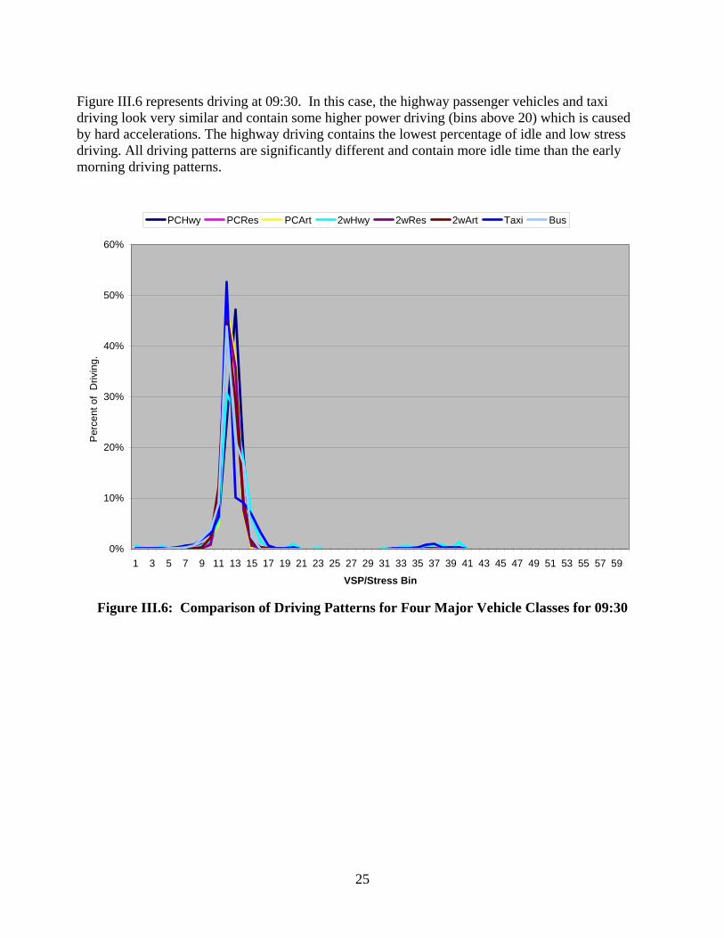
Figure III.6 represents driving at 09:30. In this case, the highway passenger vehicles and taxi driving look very similar and contain some higher power driving (bins above 20) which is caused by hard accelerations. The highway driving contains the lowest percentage of idle and low stress driving. All driving patterns are significantly different and contain more idle time than the early morning driving patterns.
Figure III.6: Comparison of Driving Patterns for Four Major Vehicle Classes for 09:30
25
Figure III.7 represents the 12:30 time frame. This hour of the day represents the most uniform driving among the various vehicle classes. Very little high stress driving is seen here. Both the 09:30 and the 12:30 driving contain much larger proportions of low stress and idle driving.
Figure III.7: Comparison of Driving Patterns for Four Major Vehicle Classes for 12:30
Data sets using the binned data and average speeds are used in the IVE model to correct emission estimates for local driving patterns.
26
IV. VEHICLE START PATTERNS2 IV.A. BACGROUND AND OBJECTIVES Between10% and 30% of vehicle emissions come from vehicle starts in the United States. This is a significant amount of emissions. Thus, it is important to understand vehicle start patterns in an urban area to fully evaluate vehicle emissions. To measure start patterns, a small device that plugs into the cigarette lighter or otherwise hooks into a vehicles electrical system has been developed. The voltage fluctuations in the electrical system can be used to estimate when a vehicle engine is on and off. This process is described in Appendix A. The main objective of this section is to collect a representative sample of the number, time of day, and soak period from passenger vehicles operating in Lima. IV.B. METHODOLOGY The vehicle engine start patterns were collected using equipment that senses vehicle system voltage denoted VOCE units. VOCE data can be used to determine when vehicles start, how long they operate, and how long they sit idle between starts. This information is essential to establish vehicle start emissions. The VOCE units were placed in passenger vehicles and left there for a week. IV.C. RESULTS Table IV.1 indicates the measured start and soak patterns for passenger vehicles in Lima. Data was successfully collected from about 80 passenger vehicles over about 4 days for each vehicle. This provides about 340 vehicle days of data. While this amount of information is significant, it was felt that hour by hour data would include too few events and would thus not be meaningful. Thus, the data was lumped into 3 hour groups.
Table IV.1: Passenger Vehicle Start and Soak Patterns for Lima Soak Time (hrs)
2 The data for this chapter is still being analyzed and the vehicle soak patterns will likely change modestly to reflect this further analysis. These changes could also slightly change the emission results, which will also be modified if needed.
27
Overall, Lima passenger vehicles were started 5.6 times per day. This is typical of what is observed in other urban areas that have been studied. Starts per day vary from 6-8 for passenger vehicles in the urban areas studied to date.3 As expected, most starts occur in the 06:00 to 09:00 time frame. The second highest number of starts is in the 15:00- 18:00 time frame, and the third in the 18:00 – 21:00 time frame. The highest fraction of starts after an 8 or more hour weight occurs in the early morning to morning time frame as would be expected. These long soak times leave the engine cold and result in much greater start emissions.
3 Studies to date have been conducted in Los Angeles, USA; Santiago, Chile; Nairobi, Kenya; and Pune, India.
28
V. IVE APPLICATION AND EMISSIONS RESULTS The total daily driving in the Lima Metropolitan Area is on the order of 70,000,000 kilometers based on the information provided to us [1]. The fraction of driving per hour can be estimated using traffic counts shown in Table II.1 and averaged according to the fraction of driving on each type of street discussed in Section II.A. Based on the observed number of vehicles on the different road types and the total length of each type of road in Lima, it was estimated that 24% of overall driving in Lima is on arterials, 69% on highways, and 7% on residential streets. The results are shown in Table V.1. Since no data was collected between 0:00 and 06:00 and between 19:00 and 0:00 these values were estimated using fractions observed in other urban areas. In the case of vehicle starts, Tables IV.1 and IV.2 were weighted by the fraction of passenger vehicles. A total of approximately 0.9 million vehicles were assumed to be in daily operation in 2003 in the Lima Metropolitan Area.
Table V.1: Estimated Fraction and VMT and Starts By Hour in Lima Metropolitan Area
Total 70,000,000 26,205,375 (data in red had to be estimated from data collected in other urban areas since these times were not observed in Lima) The calculations shown above are for illustrative purposes only. They are approximations and more extensive measurements should be completed in Lima to improve the estimate of total daily driving in Lima and hourly driving outside of the hours measured in this study.
29
No data was available concerning the technology distribution of the bus and truck diesel fleets in Lima. There has been little regulation of diesels and the diesel engine producers are international in scope. Thus, the technologies assumed for the bus and truck fleets were the same as those observed in our study in Mexico City where actual diesel engine technology data was available. This is another part of the study where improvements can be made, but it is not anticipated that there will be enough variation in the diesel fleet in Mexico City and Lima to significantly change the emission results. Figure V.1 shows the modeling results using the data developed or estimated from this study for Carbon Monoxide. The top line reflects start and running emissions added together.
Figure V.1: Overall Lima Carbon Monoxide Emissions
The peak CO emissions are occurring around 07:30 and 18:00. The minimum during the day occurs around 10:00. Off course, emissions are very low from 21:00 to 02:00. It is also valuable to note the importance of start emissions in Lima. Most of the time, they represent almost half of vehicle CO emissions. Overall, Figure V.1 reflects a total of 3524 metric tons of CO emitted per day into the air over Lima or an overall daily average emission rate of 50 grams/kilometer traveled including starting and running emissions.
30
Figure V.2 shows the modeling results using the data developed or estimated from this study for volatile organic compounds (VOC) including evaporative emissions. The top line reflects start, running, and evaporative emissions added together.
Figure V.2: Overall Lima Volatile Organic Emissions
There are two VOC peak emissions, one occurring in the morning, which could facilitate ozone formation. Start emissions are not as great a percentage of emissions as is the case for CO, but they are still large. Evaporative emissions are somewhat important as well. Figure V.2 reflects a total of 294 metric tons per day of VOC emissions going into the air over Lima or an overall daily average emission rate of 4 grams/kilometer including starting, running, and evaporative emissions.
31
Figure V.3 shows the modeling results using the data developed or estimated from this study for Nitrogen Oxides (NOx). The top line reflects start and running emissions added together. Start emissions are much lower in this case. As is the case for CO and VOC, there is a bimodal distribution of emissions with the largest peaks occurring in the morning and the afternoon. Figure V.3 reflects a total of 367 metric tons per day of NOx going into the air over Lima or an overall daily average emission rate of 5 grams/kilometer including starting and running emissions.
Figure V.4 shows the modeling results using the data developed or estimated from this study for Particulate Matter (PM). The top line reflects start and running emissions added together. Start emissions are much lower in this case although still large. Figure V.4 reflects a total of 22 metric tons per day of PM going into the air over Lima or an overall daily average emission rate of 0.30 grams/kilometer including starting and running emissions.
Figure V.4: Overall Lima Particulate Matter Emissions
Figures V.1-V.4 were calculated based on a total daily driving of 70 million kilometers and a fleet of 924,695 vehicles. The emission numbers will of course have to be modified if the total kilometers per day measured in Lima are greater than 70,000,000 and/or if the number of vehicles actually operating daily is different from 0.9 million.
33
To better understand the emissions created from the Lima vehicle fleet, it is useful to look at the contribution of each type of vehicle class. For Lima, the major vehicle categories include light duty passenger vehicles and trucks (LD), two wheeled vehicles (2w), taxis (taxis), buses (Bus), and trucks (Truck). The fraction of travel from each of these types of vehicles is shown in the last column of Figure V.5. The percent contribution each of these vehicle types to vehicular CO, VOC, NOx, and PM emissions is also shown in Figure V.5. These results indicate the majority of vehicular CO, VOC, and NOx are from buses and passenger cars.
0%
10%
20%
30%
40%
50%
60%
CO VOC NOX PM VMT
PC Taxi Buses Truck 2w
Figure V.5 Emission Contribution of Each Vehicle Type in Lima
Clearly, to reduce PM emissions in Lima, buses and trucks must be controlled. To reduce NOx, buses, trucks, and passenger vehicles must be further controlled.
34
Another calculation that is of interest is the overall per kilometer emissions of Lima vehicles compared to vehicle fleets in cities of other countries. Figure V.6 compares Lima with Los Angeles, Santiago, Mexico, Nairobi, and Pune. These locations have a very different profile of vehicle fleet, fuel type, and driving patterns.
0
2
4
6
8
10
12
14
CO/10 VOC NOx PM*10 CO2/40
Emis
sion
Rat
e (g
/km
)
Los Angeles Nairobi Santiago Pune Mexico Lima
Figure V.6: Comparison of Daily Average Emission Rates in Countries Studied to Date
The Lima fleet has the second highest emissions of both NOx and PM, and the highest CO2 emissions. It is a moderate producer of CO and VOC. The high PM emissions are particularly troubling because they suggest a commensurate high emission rate of toxics. Figures V5 and V6 illustrate the possibilities that if emission rates were lowered, significant emissions reductions could be achieved in the Lima area.
35
In conclusion, this study has developed basic data to allow for improved estimates of emissions from the Lima fleet. Additional studies are needed to further improve emission estimates in Peru, but significant planning activities can occur using the data in this report. Our recommendations are as follows:
1. Use the IVE model along with air quality measurements to map out a strategy for improved future air quality, and then seek to improve the air quality management process by further upgrading the Lima database.
2. Investigate the variations of the fleet, activity and fuel quality on areas beyond Lima if
extrapolations are to be made to the entire metropolitan area.
3. Improve emission factors for in-use vehicles. More emission studies are needed to verify the operating emissions of passenger vehicles, buses and trucks in Lima to insure that the best emission factors are being used. This research is being planned for later in 2004 for Sao Paulo and Mexico City.
4. Improve the estimate of total VMT for the entire Lima region to support overall emission
estimates. 5. Directly measure toxic emissions from these vehicles to better quantify the toxic emission
rates from these sources.
36
37
Appendix A
Data Collection Program Used in Lima
1 A.
International Vehicle Emissions Model
Field Data Collection Activities
2 A.
3 A.
Table of Contents A.I. Introduction …………………………………………………………………... A6 A.II. Collecting Representative Data ……………………………………………… A7 A.III. On-Road Driving Pattern Collection Using GPS Technology ………………. A11 A.IV. On-Road Vehicle Technology Identification Using Video Cameras ………… A15 A.V. On-Road Vehicle Technology Identification Using Parked Vehicle Surveys ... A17 A.VI. Vehicle Start-Up Patterns by Monitoring Vehicle Voltage …………….…….. A18 A.VII. Research Coordination and Local Support Needs ……………………….…… A20
4 A.
5 A.
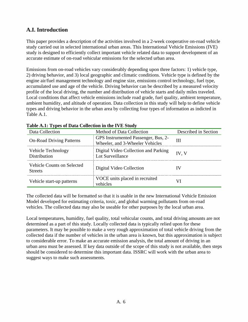
A.I. Introduction This paper provides a description of the activities involved in a 2-week cooperative on-road vehicle study carried out in selected international urban areas. This International Vehicle Emissions (IVE) study is designed to efficiently collect important vehicle related data to support development of an accurate estimate of on-road vehicular emissions for the selected urban area. Emissions from on-road vehicles vary considerably depending upon three factors: 1) vehicle type, 2) driving behavior, and 3) local geographic and climatic conditions. Vehicle type is defined by the engine air/fuel management technology and engine size, emissions control technology, fuel type, accumulated use and age of the vehicle. Driving behavior can be described by a measured velocity profile of the local driving, the number and distribution of vehicle starts and daily miles traveled. Local conditions that affect vehicle emissions include road grade, fuel quality, ambient temperature, ambient humidity, and altitude of operation. Data collection in this study will help to define vehicle types and driving behavior in the urban area by collecting four types of information as indicted in Table A.1. Table A.1: Types of Data Collection in the IVE Study
Data Collection Method of Data Collection Described in Section
On-Road Driving Patterns GPS Instrumented Passenger, Bus, 2-Wheeler, and 3-Wheeler Vehicles III
Vehicle Technology Distribution
Digital Video Collection and Parking Lot Surveillance IV, V
Vehicle Counts on Selected Streets Digital Video Collection IV
Vehicle start-up patterns VOCE units placed in recruited vehicles VI
The collected data will be formatted so that it is usable in the new International Vehicle Emission Model developed for estimating criteria, toxic, and global warming pollutants from on-road vehicles. The collected data may also be useable for other purposes by the local urban area. Local temperatures, humidity, fuel quality, total vehicular counts, and total driving amounts are not determined as a part of this study. Locally collected data is typically relied upon for these parameters. It may be possible to make a very rough approximation of total vehicle driving from the collected data if the number of vehicles in the urban area is known, but this approximation is subject to considerable error. To make an accurate emission analysis, the total amount of driving in an urban area must be assessed. If key data outside of the scope of this study is not available, then steps should be considered to determine this important data. ISSRC will work with the urban area to suggest ways to make such assessments.
6 A.
A.II. Collecting Representative Data Before the specific study elements are described, it is important to consider the overall data collection process. The IVE study is carried out over a single 2-week study period. Given that there are limited equipment and study personnel, it is not possible to collect a complete data set over an entire urban area. Thus, the study must be designed to collect representative data that can be extrapolated to the full urban area. The IVE study process has been designed with this thought in mind. On-road driving varies by the time of the day, by the day of the week, and by the location in an urban area. To account for this, during the IVE study, data is collected at different times of the day and in different locations within an urban area. This study is not designed to generally capture data on the weekend or very late at night. Thus, the study is primarily applicable to weekday driving and only limited weekend extrapolations and assumptions about traffic flow very late at night can be made. Conducting a weekend study will produce valuable information and should be considered for future research4. It should also be noted that the collected data could be improved in the future by replicating data collection activities to improve statistics, expanding the parts of the city studied, and expanding the times that are studied. Selecting Parts of a City for Study Three representative sections of the city are normally selected for the IVE study. The areas selected should represent the fleet makeup and the general driving taking place in the city. It is recommended that one of the study areas represent a generally lower income area of the city, one of the study areas represent a generally upper income area of the city, and one of the study areas represent a commercial area of the city. The sections representing the upper and lower income areas of the city for study should not be the absolute poorest or richest part of the city. It is better to select areas that are representative of the lower half of the income and the upper half of the income. Normally the urban center is selected as the best commercial area to study. Due to their much greater knowledge of their own city, it is an important role of the local partners for an IVE study to play a primary role in the selection of the three appropriate parts of the urban area to study. ISSRC is amenable to modifications in the recommended study areas due to unique situations that might occur in a particular urban area. For example, there may not be a large enough discernable upper or lower income area. The following criteria should be used as guidelines for selecting adequate sites:
♦Selection of a low income, upper income, and commercial area with a variety of streets
(i.e. residential, freeway, and arterial) in the area.
♦Accessibility to a representative parking lot or on-street parking where up to 150 parked vehicles can be studied within 10 minutes walking of each site selected.
4 In Los Angeles, some of the worst air pollution levels now occur on the weekend. This is due to the modified driving patterns and fleet mix that occurs on weekends compared to weekdays.
7 A.
Selecting Driving Routes for Study Within each of the study areas, different types of streets must be analyzed to gather data representative of all of urban streets. Streets are often classified into three general groupings. The first group represents streets that are major urban connectors and can connect one urban area to another. These streets are typically characterized by the highest traveling speed in free-flow traffic with minimal stops from cross-flow traffic and are commonly referred to as highways or freeways in some cases. The second classification of streets represents streets that connect sections of an urban area. They may connect one section of an urban area with another or may provide an important connection within a section of the urban area. These streets are typically referred to as arterials. The third classification of streets represents the streets that take people to their homes or small commercial sections of an urban area, and are usually one- or two-lane roadways with a relatively lower average speed and frequent intersections. These streets are typically referred to as residential streets. Due to time limitations, only nine street-sections can be effectively studied during the IVE project. The term “street-section” as used in this study can include parts of more than one street, but to simplify data analysis, the streets that are included within a single street-section should all be the same street classification. For example, residential streets should not be mixed with highways in a single street-section. It is important that the nine selected street sections represent each of the important street types in the urban area. The following criteria should be used as guidelines for selecting suitable street- sections:
♦For each of the street-sections, accessibility to a safe and legal location for the camera team to be dropped where 2 cameras & tripods can be set up with a clear view of the nearby traffic (tripods are approximately 0.5 meters in diameter). This location should be within approximately 5 minutes of the driving route. Preferably, the cameras will capture a portion of the driving trace5 being covered by the chase vehicles.
♦Access to the different street types in a part of the city so that the chase vehicle can move
from one street-section type to another within 10 minutes driving time. This insures that time loss in moving from the highway street-section to the residential street section to the arterial street section and back does not require too much lost driving time.
♦A driving trace for each street segment must be defined so that the driver can complete it
in 50 minutes or less under the worst traffic conditions that will be encountered during the study.
In the upper and lower income sections of the city, it is recommended that a highway street-section, an arterial street-section, and a residential street-section be selected in each of the two areas. In the commercial area it is recommended that a highway section and two arterial sections be selected for study. As noted earlier, the defined street-sections do not have to be the same street, although they should be the same classification of street for a street-section grouping. Figure A.1 shows an example of three street-segments designed for an upper-income area in Los Angeles, California.
5 A driving trace is the route followed by the chase vehicles as they drive along one of the selected street-sections.
8 A.
Figure A.1 Example of a Residential, Arterial, and Freeway Street-Segment Selected for a Single Study Area
Designing a set of interconnected arterials or residential streets that ultimately connect to one another to form a circular drive can provide an effective street-section for this study. This circular design is often not possible with highways and the driver may have to drive one way on a highway and then return on that same highway on the other side of the street. During less congested times, it is often possible that a driver can drive the designated street-section more than one time. This is not a problem and simply adds to the database during a time period. As is the case with selecting general areas of the city to study, it is an important role of the local partners to select the nine streets to be studied. ISSRC will review the nine selected street sections and make recommendations as necessary. Times of Data Collection It is also important to collect data at different times of the day to account for traffic congestion and resulting changing flow rates as the day progresses. Testing is carried out normally over a 6 day period for the collection of urban driving patterns and vehicle technology data. Since driving in difficult traffic situations and collecting on-road vehicle technologies are typically very tiring and dirty activities, data collection is held to about 7 hours each day. Since information is typically needed from 06:00 to 20:00 to understand the complete cycle of traffic flow, the driving times are
9 A.
set for 7 hours in the morning on one day of data collection and 7 hours in the evening the next day of data collection. Data collection is normally started at 06:00 and continues until shortly before 13:00 for the morning data collection and starts at 13:00 and goes to shortly before 20:00 for the afternoon data collection. If special circumstances exist in an area where data is desired at earlier or later times, this should be discussed in advance of the study period. Collecting Other Related Data Parking lot data is collected in the same parts of the city where on-road driving and technology data are collected. It is desirable to capture vehicle technologies that exist down to 1% of the fleet. To increase the probability of seeing the types of vehicles that exist at the 1% level and to improve the accuracy of vehicle use data, it is important to collect data on more than 800 randomly selected parked vehicles over the 6-day study period. Generally, it is attempted to collect data on 300 vehicles in each of the three selected sections of the urban area; however, vehicle availability in lower income sections often reduce the total collected data to 800-850 vehicles in the overall study. In the case of the collection of start-up data, individuals are asked to carry small data collection devices in their vehicles. It is important that the individuals selected for this portion of the study should be representative of the general driving population. It would be best to study at least 300 persons, but lack of time and equipment does not allow this large of a study. As discussed later in this paper, it is more efficient to collect data over more days from fewer persons. In all, it is hoped that more than 100 persons will use the units for at least 3 days per person to provide 300 person-days of information.
10 A.
A.III. On-Road Driving Pattern Collection Using GPS Technology Collection of on-road driving pattern data will be conducted on the streets identified by local agencies as discussed in Section II. This data collection will be conducted using combined Global Positioning Satellite (CGPS) modules with microprocessors developed by CE-CERT and GSSR. The unit is placed on a vehicle that drives on predetermined street sections with the flow of traffic. The CGPS module collects information about the location, speed, and altitude on a second by second basis. For areas with large passenger vehicle, bus, 2-wheeler, and/or 3-wheeler populations it is important to collect independent driving pattern data for all of these vehicles since they will likely operate differently. Eight CGPS modules will be provided for the study: three for passenger vehicles, one for a 2-wheeler, and two each for buses and 3-wheelers. An additional two units are brought as backup units. The collection procedure for each type of vehicle is described later in this section. Figure A.2 shows a typical CGPS unit. They weigh about 5.5 kilograms each and can be strapped to the back of a 2-wheeler or placed on the seat of a passenger vehicle. An antenna is required. In the case of 2-wheelers, 3-wheelers, and buses some experimentation may be required to fina a suitable location for the antenna. The antenna is magnetic and will stick to the roof of automobiles easily. In the case of buses with fiberglass roofs, 2-wheelers, and 3-wheelers tape or other attachment means may be necessary. The antenna may be taped to the top of the CGPS box, the bus roof, or may be attached to the helmet of the 2-wheeler operator.
Figure A.2 CGPS Unit
Driving Pattern Collection for Passenger Vehicles and 2-wheelers To collect general passenger vehicle driving patterns, the local partners for the study must arrange for three passenger vehicles and local drivers to drive for eight hours each day for 6 days. In addition, one CGPS unit will be dedicated to the collection of 2-wheeler data6. The local study
6 The decision to collect data from 2-wheelers and 3-wheelers is dependent upon the size fraction of these types of vehicles in the fleet. In the case of studies in the United States and Chile it was determined that 2-wheelers and 3-wheelers were too small of a portion of the fleets to justify the collection of driving pattern data for these vehicles.
11 A.
partners should identify up to six 2-wheelers and drivers to participate in this study7. Figure A.3 shows a passenger vehicle equipped with a GPS module as used in Santiago, Chile. The CGPS units do not require an operator or laptop computer. Thus, only the driver is necessary.
GPS Antenna
Laptop & Recorder
Driver
GPS Antenna
Laptop & Recorder
Driver
GPS Antenna
Laptop & Recorder
Driver
Figure A.3: GPS Instrumented Vehicle in Santiago, Chile
These drivers are asked to operate their vehicles on the nine designated street-sections (see Section II for a discussion of street-sections) over the course of the study. The purpose of the instrumented vehicle is to collect representative data concerning local passenger vehicle driving patterns. To accomplish this, the vehicle is operated on the selected street-sections in accordance with normal traffic at the time they operate. It is important that the drivers duplicate typical driving patterns for the study area. Each day, one of the instrumented vehicles is assigned to a different selected area of the city (see Section II for a discussion of the general test areas of the urban area). The vehicles will operate in their section of the urban area for two days before moving to the next selected area of the city. The first day they will operate their vehicles in the morning timeframe and the second day they will operate their vehicles in the afternoon timeframe. Each vehicle will operate on a selected street-section for 1 hour and then move to another of the selected street-section in a predetermined pattern. Since there are three street sections in an area, after the third section is reached, the driver will return to the first street section and repeat the process until the end of the 7-hour test period. Table III.1 shows the driving circuits for the three passenger vehicles and 2-wheeler. It is important that the drivers adhere strictly to the defined street-section order to insure that all times of the day are covered. The 3 parts of the urban area designated for study are denoted as Area A, Area B, and Area C. The 3 street-sections selected in each area are designated as street-section 1, 2, or 3. Thus the highway street-section in Area A is designated as Street-Section A.1 and similarly for the others.
7 It should be okay to use as few as three 2-wheelers over the course of the study. It is important to get a cross section of 2-wheeler types that represent different engine sizes. The use of 6 2-wheelers will reduce driver fatigue during the course of the study. One 2-wheeler could operate each day through the 6-day study.
12 A.
Table A.2: Passenger Vehicle and 2-Wheeler Driving Circuits Day 1
It is important that the passenger vehicle and 2-wheeler operators keep a record of the times when their driving should not be included in the analysis due to their taking a rest or leaving the study area. It is also important that the drivers note any unusual traffic conditions that would invalidate the data. Each driver is to be supplied with a writing tablet and pen in order to make records of unusual traffic situations. The CGPS unit will record information on where the driver operated the vehicle and how it was operated. Thus, data analysis will indicate if the proper driving routes were followed. Measurement of Bus and 3-Wheeler Driving Patterns In the case of 3-wheelers and buses, student participants will be asked to take passage on suitable buses and 3-wheeler vehicles operating on the street sections of interest. Four units are dedicated to this purpose. Two units will be used for 3-wheelers and two units will be used for buses8. Care should be taken to select likely bus routes and 3-wheeler routes to be used before the study begins in order to avoid lost time once ISSRC personnel reach the study area.
8 The reserve CGPS units could also be used if the local partners are willing to provide additional 2-wheelers or students to collect bus and 3-wheeler data. Of course, if a CGPS unit fails the reserve units will have to be moved to replace the failed unit.
14 A.
A.IV. On-Road Vehicle Technology Identification Using Digital Video Cameras Two digital video cameras are set up on the roadside or above the road to capture images of the vehicles driving by. This data is later manually reviewed to determine the number, size and type of vehicle. It is important to set the cameras at an appropriate height in order to have a good view of traffic on one side of a roadway. Useful data can be captured with the cameras located at the roadside, but on busy roads it is best to have the cameras elevated 1 to 3 meters above the street level when possible. Figure IV.1 shows videotaping in Santiago, Chile on a residential street. In this case due to the low traffic volume and small street size, videotaping could be carried out at street level. Figure A.4 shows videotaping from an overpass of a freeway in Los Angeles, California. In this case due to the high traffic volume and the multiple lane roadways, data is best collected from directly above the street. Data is collected on the same roads and at the same times when driving patterns are being collected. This allows driving speeds and patterns determined from the CGPS units (discussed earlier in this paper) to be correlated with traffic counts taken from the digital video cameras. Thus, selection of roadways, as discussed in Section II, should consider the video taping requirements as well.
Figure A.4: Cameras collecting data on a resident
15 A.
Detail Camera
ial roadway in S
Traffic Count Camera
antiago, Chile
Camera Setup on the Overpass Picture of the Freeway Below
Figure A.5: Camera collecting data from a freeway overpass in Los Angeles, California The digital video cameras and the two operators usually travel with one of the instrumented vehicles to their desired location. Videotapes for analysis are collected for at least 20 minutes out of each hour and preferably for 40 minutes of each hour. Local citizens passing the cameras often have questions and upon occasion, the police become concerned about the operation of the cameras. It is important to provide a local person to explain the purpose of the data collection effort to avoid raising local concerns. It should also be noted that working along side the street for up to 7 hours a day could expose the video taping crew to considerable dust and other pollutants. It is recommended that the camera operators have good quality dust masks for cases where the dust levels are high. Each day about 3.5 hours of videotapes are collected. These videotapes are analyzed the following day by student workers and ISSRC staff to develop the needed data for establishing on-road fleet fractions. ISSRC will provide two videotape readers and laptop computers to support analysis of the data during the data collection process.
16 A.
A.V. On-Road Vehicle Technology Identification Using Parked Vehicle Surveys The on-road technology identification process using digital video cameras does not collect all of the information required to completely identify the vehicle. Therefore, it is important to supplement this data by visual inspection of parked vehicles using on-street and parking lot surveys. Figure V.1 shows data collection in a Nairobi parking lot. By use of an experienced mechanic recruited from the local area, model year distributions, odometer (distance traveled) data, air conditioning, engine air/fuel control, engine size, and emissions control technology can be estimated for the local fleet using this type of survey technique. Studies in Los Angeles indicate that the technology distributions found in parking lots and along the street closely mirror the on-road vehicle fleet.
Figure A.6: Parking Lot Data Collection in Nairobi, Kenya
The determination of the needed data involves looking inside of parked vehicles. This process can alarm vehicle owners and the police upon occasion. It is important that a local person participate in the parking lot survey that can explain the purpose of the study and resolve concerns of local law enforcement officials. Surveys are conducted in the same general areas where the vehicle driving patterns are collected. The parked vehicle survey team typically rides to their daily study area with the second instrumented vehicle (the first instrumented vehicle carries the on-road camera crew). The second instrumented vehicle leaves the parked vehicle survey team at a suitable location where sufficient numbers of parked vehicles can be found. This instrumented vehicle returns at the end of the study to pick up the surveyors. As noted earlier it is desirable to collect data on more than 800 vehicles. Thus, the daily goal for the parking lot survey crew is 150 vehicles.
17 A.
A.VI. Vehicle Start-Up Patterns by Monitoring Vehicle Voltage As noted earlier, vehicles pollute more when they are first started compared to operations when they are fully warmed up. The colder the vehicle when started, the typically greater emissions. It is thus important to know how often vehicles are started in an urban area and how long a vehicle is off between starts to make an accurate estimate of start-up emissions. ISSRC will bring 56 Vehicle Occupancy Characteristics Enumerator (VOCE) units to measure the times that vehicles are started and how often. These VOCE units will also give us information on how long vehicles are typically operated at different hours of the day. Figure VI.1 shows one of the units in a typical application. It is normally plugged into the cigarette lighter in the vehicle and left there for up to a week at a time, collecting data all the while.
Cigarette Lighter Plug
t
Figure A.7: VOCE Unit for Collecting Vehicle Start Informat The VOCE units operate by simply recording vehicle voltage on a second by secovoltage rises when the vehicle is operated. Software has been developed to downldata from the units. In cases where there are no cigarette lighters, clamps are avaiclamp the VOCE units to the vehicle battery or other suitable location to capture During the study, 50 of the VOCE units will be distributed to local vehicle ownertheir vehicles for four days. The units are then retrieved, the data downloaded, an50 different vehicle owners for another four days. To complete this part of the sparticipants must be identified by the local partners to use the units by the titeam reaches the location. The VOCE units are distributed within the first 24 hothe ISSRC team. At the end of 4 days, the units are retrieved, the data downloadethe units re-distributed the next day for another 4 days. This will give us 400 persinformation. In some cases when a weekend intervenes, the units are left for morewith the vehicle owners and weekend data is collected. The VOCE units are capa
18 A.
VOCE Uni
ion
nd basis. The oad and interpret lable to directly system voltage.
s and attached to d given back out to tudy, 100 me the ISSRC urs after arrival of d over night, and on days of than four days
ble of operating
and collecting data for more than a week if necessary. There will be 6 extra VOCE units that can be used to replace units if they become faulty. In past studies, the vehicle owners have installed the units themselves since they normally only have to be plugged into the vehicles cigarette lighter and left there for the four days of data collection. In cases where the vehicle does not have a cigarette lighter, ISSRC personnel and local partners may have to help the vehicle owner to install the unit. It is important that none of the VOCE units are lost because they are each hand built and can not be easily replaced. To complete this part of the operation, one local person is normally required to spend most of their time during the testing program to first identify 100 participants in advance and then to give out and retrieve the units. Vehicle owners often forget to bring the VOCE units back when they are supposed to or have a problem that keeps them from coming to work to return the units. Thus, while simple in concept, identification, deployment and retrieval of 50 units in the proper timeframe can be a complicated and tedious process. Finally, in selecting vehicle owners to use the VOCE units it is import to select persons that represent a cross section of drivers in the urban area of interest.
19 A.
A.VII. Research Coordination and Local Support Needs In order to properly carry out the data collection and processing outlined in this paper, both ISSRC and local support are needed. ISSRC will provide 2 persons to work on the project. It is requested that the local partners supply 17-23 persons. 7-14 of these people can be students. Table A.3 below outlines the needed ISSRC and local support requirements.
Table A.3: Study Support Requirements ISSRC Support Local Support - Staff Local Support – Student
Prior to Start of the Test
Obtain needed Visas, test and pack equipment, review streets selected
by local partners.
Obtain permission to bring test equipment into the country. Identify 100 persons to participate in vehicle start pattern data
collection. Identify road sections for vehicle technology and driving pattern
measurement. Identify support staff including students, mechanics, motorcycle
owners, and chase vehicles and drivers.
On-Road Driving Patterns Researcher A: Provide training in use of GPS in chase car situations.
Support data analysis as data is collected.
3 local drivers with vehicle to collect on-road passenger car driving patterns
1 student to support data analysis process.
Researcher A: Provide training in use of GPS on 2-Wheeler, 3-
Wheeler, and Buses. Support data analysis as data is collected.
3-6 motorcycle operators for one or two days each (could be students).
3-4 students to ride in 3-Wheeler and Bus to collect driving
pattern data.
On-Road Vehicle Technology Identification Researcher B: Setup and operate video camera and help determine
best locations for videotaping.
1 person to help setup equipment and answer questions of local citizens and
police.
Researcher B: Support tape analysis and data entry as video data is
collected.
2 students to review tapes and record technology information.
Parking Lot Technology Surveys Researcher B: Provide training on parking lot surveys. Support data
analysis as data is collected.
1-2 expert vehicle mechanics to support identification of model year and engine
technology
Researcher A/B: Support data entry and analysis process.
1 person to answer questions and get permission to collect data in parking lots
and on the street.
1 student to support entry of data into the computer and early
analysis of data. Vehicle Start Pattern Measurement
Researcher A: Support distribution and retrieval of VOCE units and
down loading data.
1-2 persons to identify 100 vehicle owners to use VOCE units in advance of start of
study and to support distribution and retrieval of the VOCE units.
Researcher A/B: Support data analysis.
Total Personnel Requirements
2 ISSRC personnel 10-15 persons to support field operations 7-8 students to support data review and entry.
20 A.
As noted earlier, the typical daily schedule is from about 06:00 to 13:00 on 3 of the 6 data collection days and 13:00 to 20:00 on 3 of the 6 data collection days. The students involved in data analysis will be requested to work each day after fieldwork is conducted. A specific test schedule will be supplied for each location based on the dates of arrival of the ISSRC team members and intervening weekends. Table A.4 below provides a checklist of equipment being brought into the country. The local partner must make arrangements with customs so that this equipment can be easily brought into and out of the country.
Table A.4: List of Equipment Brought Into and Out of the Country Equipment Use Number
GPS Speed, Altitude, and Location Measurement Device
To measure traffic patterns of vehicles operating on urban streets. 10 units
VOCE Start-Up and Driving-Time monitor
To measure the typical times vehicles are started and operated in the urban
area. 56 units
Portable Computer To record data and carry out data analysis processes. 5 units
Portable Printer To print out reports 1 unit
Video Camera To record vehicle activity on selected streets. 2 units
Video Tape Reader To read tapes and display pictures on computer screens. 2 units
Commercial GPS Device To check operation of the main GPS testing units. 1 unit
Soldering Iron To repair equipment as needed. 1 unit
Electrical Meter To check and repair equipment as needed 1 unit
Commercial AA batteries For use in the VOCE units 200 units
If you have questions about the study please contact:
discuss study and use of equipment. VOCE units distributed to
first 50 participants.
1st day of on-road testing, video taping, and parking lot surveys.
2nd day of on-road testing, video taping, and parking lot surveys. Begin processing collected data.
3rd day of on-road testing, video taping, and parking lot surveys.
Process collected
data.
4th day of on-road testing, video taping,
and parking lot surveys. Process
collected data.
March 16, 2003
March 17, 2003
March 18, 2003
March 19, 2003
March 20, 2003
March 21, 2003
March 22, 2003
Sunday Monday Tuesday Wednesday Thursday Friday Saturday No field data
collection or processing.
First 50 VOCE Units
collected. Data downloaded in
the evening.
5th day of on-road testing, video taping, and parking lot surveys.
VOCE Units distributed to
2nd 50 participants as early in day as
possible. Process
collected data.
6th day of on-road testing, video taping, and parking lot surveys. Process collected data.
Process collected
data.
2nd 50 VOCE units collected
and data downloaded. Meet at about
10:00 to review data collected
and preliminary
results of the study. Depart
by van for airport in
Mumbai at about 5PM.
Depart Mumbai at
01:05 Saturday morning.
22 A.
Example of the Work Schedule for Almaty, Kazakhstan March 30,2003
March 31, 2003
April 1, 2003 April 2, 2003 April 3, 2003 April 4, 2003 April 5, 2003
Sunday Monday Tuesday Wednesday Thursday Friday Saturday Depart Los Angeles for
Almaty, Kazakhstan
Arrive Almaty,
Kazakhstan late evening.
Meet with Almaty study group at about
14:00 to discuss study
and use of equipment. VOCE units distributed to
first 50 participants
1st day of on-road testing, videotaping, and parking lot surveys.
2nd day of on-road testing, videotaping, and parking lot surveys. Begin processing collected data.
3rd day of on-road testing, videotaping,
and parking lot surveys. Process
collected data.
April 6, 2003 April 7, 2003 April 8, 2003 April 9, 2003 April 10, 2003
April 11, 2003 April 12, 2003
Sunday Monday Tuesday Wednesday Thursday Friday Saturday No field data
collection or processing.
First 50 VOCE Units
collected. Data
downloaded in the evening.
4th day of on-road testing, videotaping, and parking lot surveys.
VOCE Units distributed to
2nd 50 participants as early in day as
possible. Process
collected data.
5th day of on-road testing, videotaping, and parking lot surveys.
Process collected data.
6th day of on-road testing, videotaping, and parking lot surveys. Process collected data.
Process collected data. 2nd 50 VOCE
Units collected in the
afternoon and data
downloaded.
Meet at about 14:00 to
review data collected and preliminary
results of the study.
April 13, 2003
April 14, 2003
April 15, 2003
April 16, 2003
April 17, 2003
April 18, 2003 April 19, 2003
Sunday Monday Tuesday Wednesday Thursday Friday Saturday Depart from
Almaty, Kazakhstan
for Los Angeles in very early morning.
23 A.
Appendix B
Daily Log of the Data Collection Program Conducted in Lima
B.1
B.2
Day One (Wednesday, December 3, 2003)
Manuel Garcia, who was supposed to be the driver for Car One, had problems with his car and did not want to jeopardize the project by bringing an undependable vehicle, however, we were not informed until 05:30 when Ernesto arrived. Ernesto called a friend who came with his car. We told Ernesto and the video team to begin at the second location at 0700-0800. So, lost the opportunity for GPS and video at A1 during the 0600-0700 time period. Srta Maura A. Pizarro Cruz came on time to serve as the third bus GPS operator, however, she had not been informed and did not have the list of bus routes to be taken. So, she is accompanying Carlos A. Malpartida Dominguez on his bus routes for the day and will serve as the third bus GPS operator tomorrow. Mauricio called cars two and three at 7:15 and they had finished the first route and were beginning the second. No way to contact car one to check on them. May need to purchase a cell phone to give them so we can check on them from time to time. Am concerned about the safety of the camera team and security of the camera equipment at the residential and arterial routes in area B. Will talk with Daniel Lovera about the possibility of hiring a security guard for the two days that the cameras will be used in Area B. When traveling by taxi from the hotel to the University, Mauricio and I took GPS readings. No reason it should not be valid taxi driving data. Saved file in Lima Day One folder. At approximately 10 a.m. Mauricio received a call from Gustavo who reported the zoom was not working on one of the cameras. We agreed he should continue with only the remaining camera for the rest of the day. It turned out that Gustavo (the one I had familiarized with the cameras and tripods) had some reason to leave so he had another person named Gustavo handle the cameras and failed to show him how to focus the viewfinder. Although the titles for the occupancy camera were provided just like those for the counter cameras, the counter titles were used for the two video's (0700-0800 & 0800-0900) that were filmed using the occupancy camera. The label on the film cassette is correct but, the 10-second video titles are incorrect because they indicate the film is from the “counter” camera. Santos reported that he had to make a modification to the residential route for the low-income area since one of the streets turned out to be one-way. We will inform the others in the morning and have them adjust their maps as well. Talked with Daniel and he says we will have 10 mechanics and 10 students performing the parking lot surveys on Friday and Sunday. In the low-income area, he is going to inform the local police of the work that we are doing and ask that they keep an eye on the video team. When downloading the GPS data collected during the day, CGPS unit 5, would not download using the download macro. It was downloaded after querying the settings and using the retrieve data setting. As a result, unit 5 was pulled from active use and Carlos (Bus 2) will be given unit 7 tomorrow.
Day Two (Thursday, December 4, 2003) Gustavo, who is doing the video taping, was late and held up Car One for area B. At 9 am, Mauricio received a call from Gustavo, the video camera operator, indicating that he felt the schedule was in error and had started videotaping on B1 during the first hour instead of B2 as the schedule calls. He had also convinced Ernesto and Rosemery to change. As a result, the first three hours on routes in area B and Area A were not done in accordance with the schedule. Santo followed the schedule, so area C should be okay. On route B, the data from the previous day was repeated for the first two hours and no data was collected during the third hour. On route A, Rosmery repeated the previous days' schedule for the first three hours. Part way through the third
B.3
hour, she learned of the error. She then went to the route that was on the schedule for hour three and collected 5 minutes of data before the end of the hour. She then proceeded in accordance with the schedule for the rest of the day. Car One (route B) experienced a mechanical malfunction. As a result, data was only collected for one circuit of route B1 (approx 4 min) and no data was collected during the last hour. Since the video cameraman is transported by Car One, no video was taken during the last hour (1200-1300) either. Thus video taping was done at the wrong locations for the first two hours, no video taping was done during the third hour, video taping was done at the correct locations (in accordance with the schedule) for hours 0900-1000, 1000-1100, and 1100-1200, and no video taping was done during the last hour. The three bus riders (Luis, Carlos, and Maura) started on time and, on their own, decided to collect more data than scheduled. They returned in the 2000 to 2100 time period. Luis had an interesting experience. He was 5 minutes into one bus route when the bus was pulled over by the police and the driver and the passengers were ordered to get off the bus. Luis refused to do so and told the police he was engaged in an environmental study for the university. The policeman told Luis he should hire a private bus and not use a public bus for the study. Luis told him the whole point of the study is to get data on public buses and continued to refuse to stop sampling and get off the bus. Ultimately, the policeman made a phone call and then told the driver and the passengers to get back on the bus and to proceed so the data collection could continue. The driver was very happy that the bus was allowed to proceed and thanked Luis profusely. Mauricio gave a very good seminar (with especially nice power point graphics) that lasted from 1800-1930. It was attended by students as well as people from other institutes/agencies. Mr. Cesar Ramirez, from SENATI, was in attendance and promised that he would have 10 mechanics available to work on the parking lot survey on Saturday and Sunday. After Mauricio’s seminar concluded, Mr. Ramirez provided some training to 20 students that are going to be assisting the mechanics on the surveys (10 on Saturday and 10 on Sunday.
Day Three (Friday, December 05, 2003) Began to download VOCE as units came in. Pretty rushed time since they came in pretty late and needed to get back out right away. Mauricio and I divided up the tasks and he went back to the hotel to provide the CGPS and camera equipment to the people for Cars 1,2,3 and Bus3. We brought two CGPS units to the university to give to Luis and Carlos for Buses 1 and 2 so they would not have to travel to the hotel. To speed the download process up, I began to use Jim’s smaller Sony. The night before, I thought I had been successful in telling the program to send the data to the VOCELima1 folder on the desktop. After downloading the first group that came in. I could not locate the data that had been downloaded on the smaller Sony. When I queried the send file, it indicated the data had been sent to a file on the desktop that is entitled, “VOCE 11-25-03.” There is no file by that name on the desktop. There is a file with that name in the recycle bin but, it has no data in it. Both Mauricio and I tried various ways to locate the data but, to no avail. There is a file listed as wbemcore that seems to indicate it tried to do something with files but, there doesn’t seem to be any data associated with it. This file can be found at C:\WINNT\system32\wbem\Logs. We later were able to determine, through a process of elimination, that the units involved were units 4, 6, 8, and 10. I then input the order for the program to send the data to the VOCELima1 file and successfully downloaded two files into it. The third unit (014A) that I tried to download on that computer, seemed to run forever and the data looked very suspicious. I finally pulled the plug out of the unit.
B.4
It continued to log data for quite a while after. Unit 014A was placed on the “needs repair” pile and taken out of service. At this point, I decided not to use the small Sony any longer. I transferred the files from the two that had successfully downloaded to the main VOCELima1 file on the large Sony. I pulled the batteries out unit 014A and let it sit for over half of an hour. When I attempted to download it again, it did the same thing. When attempting to download the information from Unit 30, the program would recognize it but, would only indicate the unit id. After just a moment, it indicates it no longer has a connection with the unit. Units 25 and 28 failed to connect with the program. All four (14, 25, 28, and 30) were pulled from service. After downloading more of the incoming VOCE data, we noticed that Mauricio’s computer was indicating Dec 6th instead of Dec 5th. So, there are some in the file that erroneously show Dec 6th as the download date instead of the 5th. Mauricio then corrected the date on his computer. Later, a couple of VOCE units seemed to act similar to 014A but, did eventually come to an end and showed the recording blocks had been reset. So, I decided to give 14 another try and to just let it download for a longer time. When I checked it later it had downloaded over 600 kbs of data (stored as unit14b) and started to recycle. I saved 14b along with 14a but when I looked at the end of the file, it indicates the unit entered its low power mode. I do not expect the data is valid. A total of 9 VOCE units were not returned by the end of the day (units 26, 29, 41, 47, 48, 49, 59, 61, and 64). We suggested that the individuals continue to keep them in their vehicles and we will collect them with the others on Thursday of next week.
Day Four (Tuesday, December 9, 2003) Only had cars 1, 2, and 3, equipped with CGPS units. All three got off on time in the early morning. Later received a call that Car 1 had broken down and Ernesto arranged for another to take its place. As a result, they were only able to get about 8 minutes of route driving during one of the hours. Since the video team uses Car 1 for transportation, they ended up taking a taxi to the next location. Due to the delay, only 15 minutes of video was collected instead of the normal 20. Car 3 was working in the low income area and had a flat tire due to nails in the road. It occurred very close to a tire repair shop and, as a result, very little time was lost. Jim tried to recover the VOCE data from units 2, 4, 6, and 10, but it does not appear to be recoverable. At 6 pm, Jim gave a presentation on the IVE model. We seem to be getting behind in having the vehicle counts completed for the videos. Silvia went with the camera crew and was unavailable for viewing the videos. Maura is going to work on videos in the morning before she leaves with the CGPS unit to monitor bus drivign activity. Took Jim to the airport for his flight to Rio de Janiero. All 10 CPGS units were charged during the night.
Day Five (Wednesday, December 10, 2003) Mauricio and I met with Carlos Hernando and Marta Valencia at the Tata taxi company in Surco. They agreed to put 5 VOCE units (#’s 65, 66, 67, 68, and 70) on 5 of their taxis and keep them on until Friday morning. We will then catch a cab to the company’s office and pick them up. They hid the units up under the dash and secured them with tape. They are interested in finding out how much time the cabs are turned off and I told them we will provide them with the information once we have assessed the data. Carlos indicated that the average daily kilometers traveled by his taxis (they have more than 100) is 450. They work two 12-hour shifts per day. Later in the day, we spoke with a taxi driver who said that during his 12 to 16 hour days he averages 240 kilometers. He
B.5
also verified what Willi had said that all of the station wagon taxis are diesel and most, if not all, of the sedan taxis are diesel because gasoline is so expensive. We staged out of the university instead of from the hotel. As normal, CGPS units 1, 2, and 3 were given out for Cars 1, 2, and 3, respectively. As in the previous days, CGPS units 4, 6, and 7 were given out for buses 1, 2, and 3, respectively. Shortly after leaving the university, Santos called to say that when he opened his case (CGPS 2) the switch was found to be on. Both Mauricio and I were sure the switch had not been on during the night while the unit was charging and felt it was something that had occurred within a short time before it was noted. As a result, we told Santos to just go on to his route and begin with his data collection. CGPS units 9 and 10 were given to Helga who is taking them to a waste management company where they will be put on a couple of waste hauling trucks and returned later in the evening. I asked Helga to be sure to find out information on the size of the trucks, the engines, etc. Mauricio gave a good seminar on the IVE activity study process at approximately 10 am. During the seminar, Cesar Ramirez, from SENATI, observed that we should have some activity data for the Combi’s since they make up a large part of the on-road vehicle fleet. Carlos and Luis have agreed to carry CGPS units on Combi’s for most of the day tomorrow. Mauricio gave a presentation at Protransporte at 3 pm. While there, we received a call indicating that the bus that Carlos had been riding in had hit a tree and the CGPS antenna apparently received some damage since it could no longer acquire satellites. We asked him to return to the university. Protransporte provided some inventory information on the Lima vehicle fleet. We have a meeting on Thursday with Cesar Ramirez at SENATI to see what vehicle inventory information he has available. We returned to the hotel from Protransporte for a short breather prior to making another trip to the university. Maura worked on the video tapes until she had to leave with the CGPS unit and ride buses. Nady came in and worked on video tapes. I discovered that she has not been recording the hours during which the video segments were made. I went back through the videos and determined the hours. I also noted that the times she had recorded for the lengths of each video segment were not as accurate as we would like and corrected. Flor volunteered to help with making the vehicle counts from the videos. We expect to have Maura, Silvia, Flor, and Nady available tomorrow. As a result, we are hoping to get the backlog caught up. Apparently the bus that Carlos had been riding in had gone under a low-hanging limb that knocked the antenna off of the roof. I replaced the antenna and the unit (CGPS unit 7) quickly acquired satellites.
Day Six (Thursday, December 11, 2003) Luis and Carlos came to the hotel at 5 am and picked up CGPS units 4, 5, 6, and 7. They are taking units 5 and 6 somewhere to be placed in trucks. Luis will take unit 4 and Carlos will take unit 7 and they will each ride around in Combi’s until mid afternoon. Around 7 am we received a phone call from Silvia Iglesias (the director of the college of geology) reporting that she had been robbed while stopped in her car and the VOCE unit she had placed in her car was one of the items taken. It is VOCE unit 21. Later, we provided her with a description of the VOCE unit so that she could include it in her report to the police. We are hoping that this police report will satisfy the customs officials when they find that I am leaving with fewer units than I brought into Peru. We conducted a comparative test for the video readers. It turned out to be a very instructive lesson and one that I would recommend be done at the beginning of every activity study from now on. The results are shown in an excel spreadsheet entitled “Limavideocomparison.” Maura, Flor, and Nady are taking turns on the video readers. Rosmery came in early to pick up her CGPS unit (unit 3) since her route today is the farthest away. Cars 1 and 2 picked up their CGPS units (units 1 and 2) between 12:30
B.6
and 1 pm. Mauricio provided me with digital maps showing the three areas and their routes. VOCE unit 4 came in but, it will not connect with the program. Both Mauricio and I tried it on our computers with no success. Removed batteries and placed in case with others. Spent a couple of hours at SENATI. Cesar is going to try to get us some vehicle data from the auto manufacturer’s association to give to us tomorrow. Cesar and the chief engineer at the inspection station indicated that 100% of the station wagon vehicles are diesel and have 2-liter engines. 65% of the gasoline vehicles have 1.5-liter engines. Since 1996, used vehicles were allowed to be sold in Peru. One of the documents provided indicates that 65% of the vehicles sold in 1998 were used vehicles coming in from other countries (mainly Japan and Korea). One of the documents received from SENATI says there are 690,000 vehicles in Lima/Callao with an average fleet age of 18 years. We were shown a video that indicated there are 650,000 vehicles in the fleet of which the medium sized buses (omnibus) average 18 years of age, the small sized buses (microbus) average 15 years, and the combi’s (camioneta rural) average 10 years. The buses are used 14 to 16 hours per day. There was a reference indicating that the combi’s average 7.3 seconds of travel time between stops. Of the total vehicle fleet in Peru, 67% are in Lima. On the return trip to the university we queried the driver. He indicated that he worked 12 hours per day and averaged 200-220 kpd. He does not stop and wait for passengers to come to him, he is always driving around looking for potential passengers. We began downloading VOCE units upon return to the university. VOCE unit 3 only gives the id and then disconnects just like unit 30 did earlier. CGPS unit 5 indicates the software connects with the unit but, like before, the macro won’t download. I attempted the manual process for downloading like I did on the first day but, with no success. We will bring the unit back to the US and attempt to recover when there is more time available. Every one of the VOCE units that were downloaded using the small Sony continue to recycle when they reach the end of the data. I think it is something in the program itself that is on that computer. None of the ones downloaded on the other computers experienced cycling. Ernesto (car one) indicated that he lost satellite signals for 15 minutes during his route in car 1, maybe due to the buildings.
Day Seven (Friday, December 12, 2003)
Picked up the 5 VOCE units (65, 66, 67, 68, 70) at Tata Taxi. Paid $25 ($5 per taxi). Carlos and Marta are really nice folks and we have found that Tata taxi is a very respected taxi company. They provided data on the taxi’s in which the VOCE units were placed and on the start and stop times. One driver pulled the plug out of the cigarette lighter and then put it back in so, those times were recorded and provided. During the drive back to the university, we queried the Tata driver. He said that he works 12 hours and that if he does not have a client and has not been asked to drive to pick up a client by the Tata central operator, he drives around looking for clients. As a result, the taxis are generally on the move all the time. Gustavo told Mauricio that he had given two VOCE units to a friend and he forgot to get the units back this morning. As a result the friends went off to their work with the units still in their vehicles. Mauricio ended up paying for a taxi so Gustavo could go to their work place and pick up the units. Flor, Maura, Rosmery, and Ernesto are working in rotation on inputting the data from the technology surveys. Later, Gustavo joined in to help on inputting the technology data. Maura and Nady are doing the video counts. Helga returned with news that the women at the Ministry of Transporte and Communications had told her to come back at 5 this afternoon to pick up the units that were in the cars of the volunteers from their agency. This is in spite of the fact that we made it clear they should recover the units on Thursday evening since we had to download them early on Friday in order to get packed up on time. Mauricio called
B.7
them and spoke with their boss and made her aware of the problem. She said she would locate the seven VOCE units and arrange that we can go to pick them up at three pm. At this point, we still have 14 VOCE units that have not been returned in addition to the one that was stolen. Daniel came and asked Nady to stop reading the video and to go to the Catholic university to pick up a VOCE unit (unit 23) that he had given someone he knows there. She came back and indicated that he had not given the person any instructions so he had simply thrown the paper away. As a result, she did not have any information on the start time. She unplugged the unit from the car and recorded the stop time. She also noted that the car is a Daewoo Tico. Later, Daniel said that he put the unit in the car and so he knows the start time. Helga is supposed to be logging in all the VOCE information so it should be in there, however, I think the start time is probably suspect. They are inputting the technology data but, it does not look like the work will be done in time before I have to leave. In that case, I will take what is done and the raw data and pack up to get to the airport. At 4:45 pm, Helga brought in the last of the VOCE units. She reported that units 15 and 43 had not been operated. Downloaded last of VOCE units. Looks like we received data from 50 units in the second phase. The students are not going to get all of the technology data logged. We are having them copy the remaining data sheets. I will take the originals and leave them the copies. I will ask that they complete the data logging and send to me via email. Just in case they don’t, we will have the original log sheets to work off of. Mauricio has written a message to Arnold Millet at Protransporte that contains photos of examples of each size of truck and bus that we are identifying in our video counts. Arnold is going to try to get us engine size and technology information and send it to me via email. One 20-minute segment on one of the three video tapes will not be done before I have to leave. It is 11 December, 2003, Route C3 from 1600-1700.