Purified Sentiment Indicators for the Stock Market...

0

Purified Sentiment Indicators

For The

Stock Market By

David R. Aronson, adjunct Professor of Finance, Baruch College Hood River Research, Inc.

&John R. Wolberg, Professor of Mechanical Engineering, Technion, Haifa Israel

POB 1809 Madison Square Station, New York, New York

10159

1

Purified Sentiment Indicators for the Stock Market

Abstract We attempt to improve the stationarity and predictive power of

stock market sentiment indicators (SI) by removing the influence of the market’s recent price dynamics (velocity, acceleration & volatility). We call the result a purified sentiment indicator (PSI). PSI is derived with an adaptive regression model employing price dynamics indicators to predict SI. PSI is the difference between observed SI and predicted SI normalized by model error. We produce PSI for the following SI: CBOE Implied Volatility Index (VIX), CBOE Equity Put to Call Ratio (PCR), American Association of Individual Investors Bulls minus Bears (AAII), Investors Intelligence Bulls minus and Bears (INV) and Hulbert’s Stock Newsletter Sentiment Index (HUL). All SI series are predictable from price dynamics (r-squares range from .25 to .70). Using cross-validation we derive a signaling rule for each SI, PSI, and price dynamics indicator and compare them with a random signal in terms of their out-of-sample profit factor (PF) trading the SP500. Purification generally improves the stationarity of SI by reducing drift and stabilizing variability. However, it generally reduces PF for PCR, AAII, INV and HUL suggesting at least some of their predictive power stems from price dynamics. In contrast, PF of VIX is significantly enhanced by purification implying it contains predictive information above and beyond price dynamics but which is masked by price dynamics. Purified VIX is superior to all other indicators tested.

I. Background

A. Sentiment Indicators Technical analysts use SI to gauge the expectations of various groups of market participants, predict market trends and generate buy & sell signals under the assumption that they carry information that is not redundant of price indicators. SI are interpreted on the basis of Contrary Opinion Theory which suggests that if investors become too extreme in their expectations,

2

the market will subsequently move opposite to the expectation. Thus, extreme levels of optimism (pessimism) should precede market declines (advances). There are of two types of SI: direct and indirect. Direct indicators poll investors in a particular group, such as individual investors (AAII) or writers of newsletters (INV & HUL) about their market expectations. Indirect indicators (PCR &VIX) infer the expectations of investors in a particular group by analyzing market statistics that reflect the group’s behavior. For example, put and call option volumes reflect the behavior of option traders. Thus an abnormally high ratio of put to call volume would imply options traders expect the market to decline.

B. Prior Research

Influence of Market Dynamics Our study is motivated by three areas of prior research: (1) influence of market dynamics on sentiment indicators, (2) predictive power of sentiment indicators and (3) use of regression analysis to purge indicators of unwanted effects in an effort to boost their predictive power. With respect to (1), intuition alone would suggest that sentiment should be influenced by the market’s recent behavior. A down (up) trend should fuel pessimism (optimism). This is supported by studies demonstrating that people suffer from an availability bias, the tendency to overestimate the probability of an event which is easily brought to mind due to recency or vividness. Thus, investors would likely overestimate the probability that a recent trend will continue. Empirical support can be found in Fosback (1976), Solt & Statman (1988), De Bondt (1993), Clarke and Statman (1998), Fisher and Statman (2000), Simon and Wiggens (2001), Brown & Cliff (2004) Wang, Keswani & Taylor (2006).

3

Tests of Predictive Power Tests of SI predictive power are numerous but inconsistent. However, because the studies consider different SI, historical periods, and evaluation metrics, a firm conclusion is difficult. Two evaluation methods have been used: correlation and the profitability of rule-based signals. Correlation quantifies the strength of the relationship between sentiment and the market’s future return in terms of r-squared, which is the percentage of the variation in return that is predicted by the SI. The signal approach measures the financial performance of sell (buy) signals given when the indicator crosses a threshold indicating excessive optimism (pessimism). Here a useful metric is the profit factor, the ratio of gains from profitable signals to losses from unprofitable signals. It implicitly takes into account the fraction of profitable signals and the average size of wins and losses. Values above 1.0 indicate a profitable rule, while values less than 1.0 indicate an unprofitable rule. Because market conditions over a given test period can profoundly impact the profit factor, an important benchmark for comparison is the profit factor of a similar number of random signals over the same time period. Using both methods, Fosback (1976) tests numerous sentiment indicators on data from 1941 through 1975, finding that some are predictive individually and conjointly when used in multiple-regression models. Solt & Statman (1988) test INV from 1963 to 1985 and find no predictive power, and attribute a pervasive belief in INV’s efficacy to cognitive errors (confirmation bias and erroneous intuitions about randomness). Clark & Statman (1998) use an additional ten years of data and confirm INV’s lack of utility. Fisher & Statman (2000) confirm this result but find that AAII is predictive. They use multiple regression to combine several SI and obtain an r-squared of 0.08 which has economic value in market timing. Simon & Wiggens (2001) use data from 1989 to 1998 to show that VIX and S&P100 option put-to-call ratio are statistically significant predictors of S&P500 over 10 to 30 days forward and derive an effective signaling rule. They conclude the SI examined frequently have statistically and economically significant predictive value. Hayes (1994) combines stock market sentiment with that of gold and treasury bonds to form a composite SI for

4

stocks and finds rule-based signals that are useful. In contrast, Brown and Cliff (2004) tested ten SI observed monthly from 1965 to 1998, and weekly from 1987 to 1998 and find that used individually or combined they have limited ability to predict near-term market returns. Wang, Keswani & Taylor (2006) test OEX put-to-call volume ratio, OEX put-to-call open interest ratio, AAII and INV using regression and find no predictive power. Clearly, the evidence is mixed.

Regression Modeling for Indicator Purification Indicator purification via regression modeling is introduced by Fosback (1976). He finds sentiment of odd-lot short sellers and mutual fund managers is predictable and that they have enhanced forecasting significance when they deviate from predicted levels. The Fosback Index (FI) is the deviation of mutual fund cash-to-asset ratio (CAR) from a regression model’s prediction based on short-term interest rates. FI signals are superior to CAR. Goepfert (2004) applies Fosback’s method to more recent data, confirming the relation between short-term interest and CAR (r-squared 0.55) and the potency of FI signals. Merrill (1982) uses regression to remove the effect of beta from a stock’s relative strength ratio (RS). A limited test shows purified RS signals are superior to those obtained from traditional RS. Jacobs and Levy (2000), use multiple regression to purify 25 fundamental and technical indicators and demonstrate that the purified indicators have improved predictive power and independence. Stonecypher (1988) derives an “available liquidity” indicator, the deviation of stocks prices from a regression prediction based on mutual fund cash, credit balances and short interest.

C. How This Paper Extends Prior Research Our research extends prior research in several ways. First, we apply regression purification to five SI not previously treated in this manner. Second, while prior studies use static regression models, ours is adaptive, with periodic refitting to allow changing indicators and indicator weights to capture changes in the linkage between market dynamics and

5

sentiment. Third, while prior studies have established the link between price velocity and SI, our study also considers acceleration and volatility. Fourth, unlike prior studies using regression for purification, we normalize the deviation between observed and predicted sentiment by the model’s standard error, thus producing an indicator with more stable variance. Fifth, prior efforts to reduce drift and stabilize the variability of SI use the trend and variability of the SI itself. Instead we use the stock market’s price dynamics because of their established influence on sentiment.

II. Analysis Procedure

A. Sentiment Indicators Analyzed

American Association of Individual Investors Sentiment Survey (AAII): July 27, 1987 to October 31, 2008, published weekly. Source Ultra Financial Systems (www.ultrafs.com)

Investors Intelligence Advisor Sentiment Bulls - Bears (INV): January 4, 1963 to October 31, 2008, published weekly by Investor’s Intelligence.

Hulbert Stock Newsletter Sentiment Index (HUL): January 2, 1985 to October 31, 2008, published weekly, is the average recommended stock market exposure for a subset of short-term market timers tracked by the Hulbert Financial Digest. Source: Mark Hulbert. CBOE Equity Put to Call Volume Ratio (PCR): October 1, 1985 through October 31, 2008. Series includes ETF options. Source: Luthold Group.

CBOE Implied Volatility Index (VIX): January 2, 1986 through October 31, 2008. It is an indicator of the implied volatility of SP500 index options. Prior to 2003 it was based on S&P100 options. Source: Ultra Financial Systems (www.ultrafs.com).

6

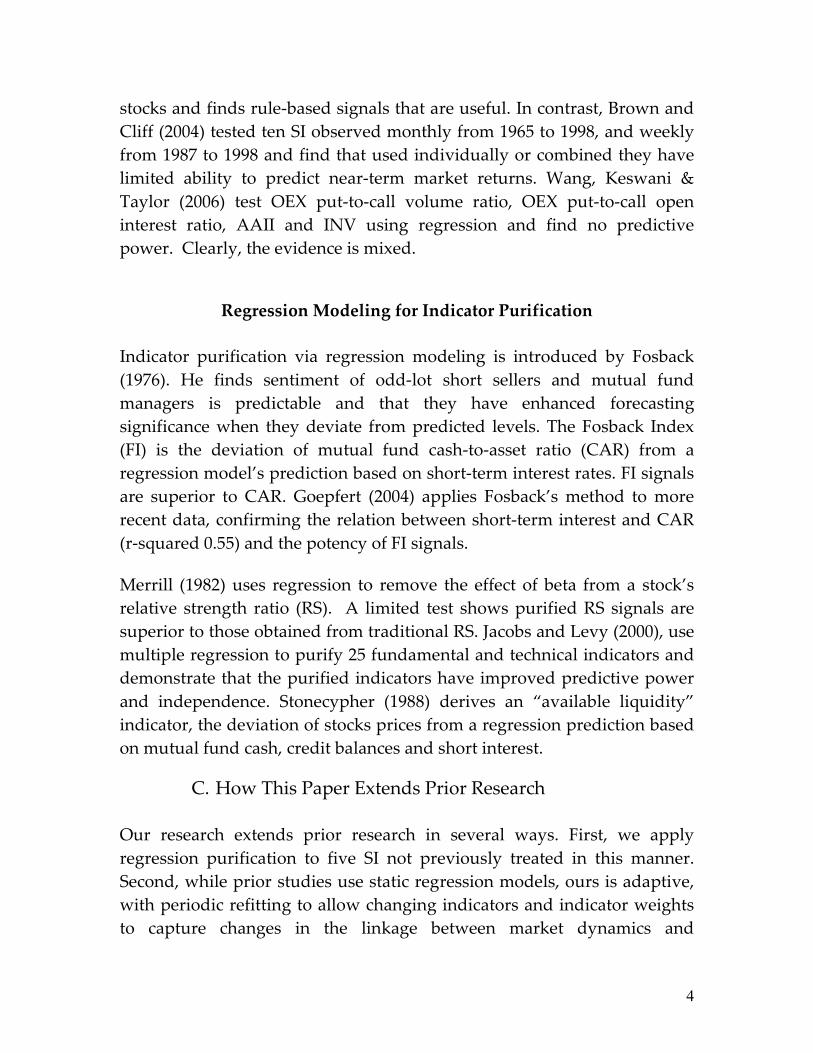
B. Method Used To Derive Purified Sentiment Indicators The conceptual basis of our purification method is seen in Figure 1, a scatterplot of velocity (price dynamics) versus a sentiment indicator. Each point on the plane is a combination of sentiment and velocity.

PriceVelocity

Optimism

Pessimism

V

Current Observation

PredictedSentiment

givenVelocity “V”

DeviationObserved

Vs.Predicted

Fig. 1

SentimentIndicator

ObservedSentiment

+-

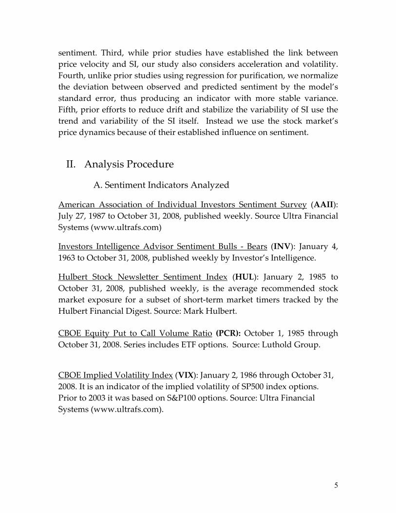
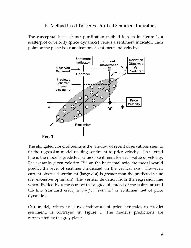
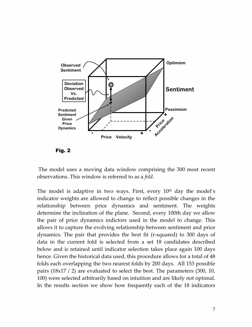
The elongated cloud of points is the window of recent observations used to fit the regression model relating sentiment to price velocity. The dotted line is the model’s predicted value of sentiment for each value of velocity. For example, given velocity “V” on the horizontal axis, the model would predict the level of sentiment indicated on the vertical axis. However, current observed sentiment (large dot) is greater than the predicted value (i.e. excessive optimism). The vertical deviation from the regression line when divided by a measure of the degree of spread of the points around the line (standard error) is purified sentiment or sentiment net of price dynamics. Our model, which uses two indicators of price dynamics to predict sentiment, is portrayed in Figure 2. The model’s predictions are represented by the grey plane.

7

Price Velocity

Price

Accelera

tion

Pessimism

Optimism

Sentiment

Fig. 2

+-

+

-

PredictedSentiment

GivenPrice

Dynamics

ObservedSentiment

DeviationObserved

Vs.Predicted

The model uses a moving data window comprising the 300 most recent observations. This window is referred to as a fold.

The model is adaptive in two ways. First, every 10th day the model’s indicator weights are allowed to change to reflect possible changes in the relationship between price dynamics and sentiment. The weights determine the inclination of the plane. Second, every 100th day we allow the pair of price dynamics indictors used in the model to change. This allows it to capture the evolving relationship between sentiment and price dynamics. The pair that provides the best fit (r-squared) to 300 days of data in the current fold is selected from a set 18 candidates described below and is retained until indicator selection takes place again 100 days hence. Given the historical data used, this procedure allows for a total of 48 folds each overlapping the two nearest folds by 200 days. All 153 possible pairs (18x17 / 2) are evaluated to select the best. The parameters (300, 10, 100) were selected arbitrarily based on intuition and are likely not optimal. In the results section we show how frequently each of the 18 indicators

8

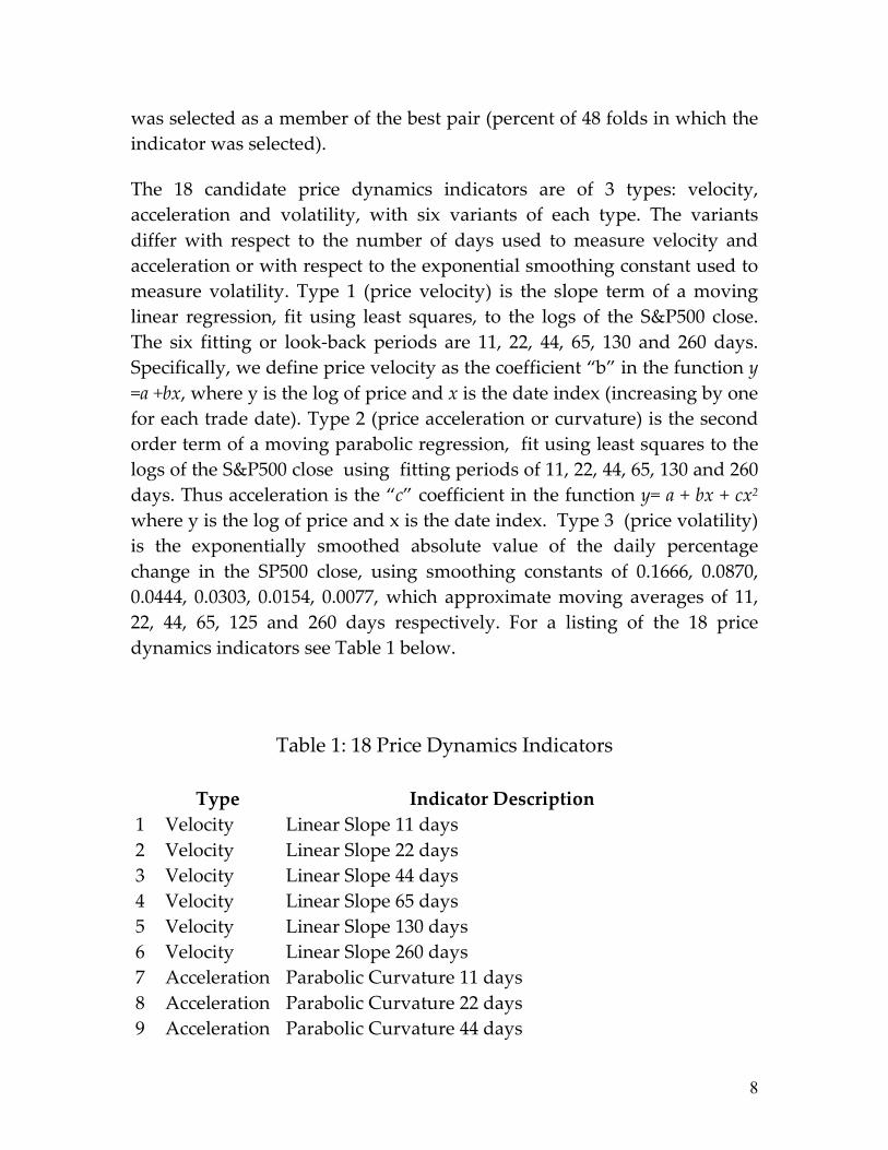
was selected as a member of the best pair (percent of 48 folds in which the indicator was selected). The 18 candidate price dynamics indicators are of 3 types: velocity, acceleration and volatility, with six variants of each type. The variants differ with respect to the number of days used to measure velocity and acceleration or with respect to the exponential smoothing constant used to measure volatility. Type 1 (price velocity) is the slope term of a moving linear regression, fit using least squares, to the logs of the S&P500 close. The six fitting or look-back periods are 11, 22, 44, 65, 130 and 260 days. Specifically, we define price velocity as the coefficient “b” in the function y=a +bx, where y is the log of price and x is the date index (increasing by one for each trade date). Type 2 (price acceleration or curvature) is the second order term of a moving parabolic regression, fit using least squares to the logs of the S&P500 close using fitting periods of 11, 22, 44, 65, 130 and 260 days. Thus acceleration is the “c” coefficient in the function y= a + bx + cx2

where y is the log of price and x is the date index. Type 3 (price volatility) is the exponentially smoothed absolute value of the daily percentage change in the SP500 close, using smoothing constants of 0.1666, 0.0870, 0.0444, 0.0303, 0.0154, 0.0077, which approximate moving averages of 11, 22, 44, 65, 125 and 260 days respectively. For a listing of the 18 price dynamics indicators see Table 1 below.

Table 1: 18 Price Dynamics Indicators

Type Indicator Description 1 Velocity Linear Slope 11 days 2 Velocity Linear Slope 22 days 3 Velocity Linear Slope 44 days 4 Velocity Linear Slope 65 days 5 Velocity Linear Slope 130 days 6 Velocity Linear Slope 260 days 7 Acceleration Parabolic Curvature 11 days 8 Acceleration Parabolic Curvature 22 days 9 Acceleration Parabolic Curvature 44 days

9

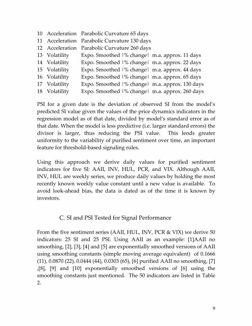
10 Acceleration Parabolic Curvature 65 days 11 Acceleration Parabolic Curvature 130 days 12 Acceleration Parabolic Curvature 260 days 13 Volatility Expo. Smoothed |% change| m.a. approx. 11 days 14 Volatility Expo. Smoothed |% change| m.a. approx. 22 days 15 Volatility Expo. Smoothed |% change| m.a. approx. 44 days 16 Volatility Expo. Smoothed |% change| m.a. approx. 65 days 17 Volatility Expo. Smoothed |% change| m.a. approx. 130 days 18 Volatility Expo. Smoothed |% change| m.a. approx. 260 days

PSI for a given date is the deviation of observed SI from the model’s predicted SI value given the values of the price dynamics indicators in the regression model as of that date, divided by model’s standard error as of that date. When the model is less predictive (i.e. larger standard errors) the divisor is larger, thus reducing the PSI value. This lends greater uniformity to the variability of purified sentiment over time, an important feature for threshold-based signaling rules. Using this approach we derive daily values for purified sentiment indicators for five SI: AAII, INV, HUL, PCR, and VIX. Although AAII, INV, HUL are weekly series, we produce daily values by holding the most recently known weekly value constant until a new value is available. To avoid look-ahead bias, the data is dated as of the time it is known by investors.

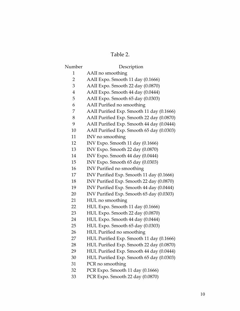
C. SI and PSI Tested for Signal Performance From the five sentiment series (AAII, HUL, INV, PCR & VIX) we derive 50 indicators: 25 SI and 25 PSI. Using AAII as an example: [1]AAII no smoothing, [2], [3], [4] and [5] are exponentially smoothed versions of AAII using smoothing constants (simple moving average equivalent) of 0.1666 (11), 0.0870 (22), 0.0444 (44), 0.0303 (65), [6] purified AAII no smoothing, [7] ,[8], [9] and [10] exponentially smoothed versions of [6] using the smoothing constants just mentioned. The 50 indicators are listed in Table 2.

10

Table 2.

Number Description 1 AAII no smoothing 2 AAII Expo. Smooth 11 day (0.1666) 3 AAII Expo. Smooth 22 day (0.0870) 4 AAII Expo. Smooth 44 day (0.0444) 5 AAII Expo. Smooth 65 day (0.0303) 6 AAII Purified no smoothing 7 AAII Purified Exp. Smooth 11 day (0.1666)8 AAII Purified Exp. Smooth 22 day (0.0870)9 AAII Purified Exp. Smooth 44 day (0.0444)10 AAII Purified Exp. Smooth 65 day (0.0303)11 INV no smoothing 12 INV Expo. Smooth 11 day (0.1666) 13 INV Expo. Smooth 22 day (0.0870) 14 INV Expo. Smooth 44 day (0.0444) 15 INV Expo. Smooth 65 day (0.0303) 16 INV Purified no smoothing 17 INV Purified Exp. Smooth 11 day (0.1666) 18 INV Purified Exp. Smooth 22 day (0.0870) 19 INV Purified Exp. Smooth 44 day (0.0444) 20 INV Purified Exp. Smooth 65 day (0.0303) 21 HUL no smoothing 22 HUL Expo. Smooth 11 day (0.1666) 23 HUL Expo. Smooth 22 day (0.0870) 24 HUL Expo. Smooth 44 day (0.0444) 25 HUL Expo. Smooth 65 day (0.0303) 26 HUL Purified no smoothing 27 HUL Purified Exp. Smooth 11 day (0.1666)28 HUL Purified Exp. Smooth 22 day (0.0870)29 HUL Purified Exp. Smooth 44 day (0.0444)30 HUL Purified Exp. Smooth 65 day (0.0303)31 PCR no smoothing 32 PCR Expo. Smooth 11 day (0.1666) 33 PCR Expo. Smooth 22 day (0.0870)

11

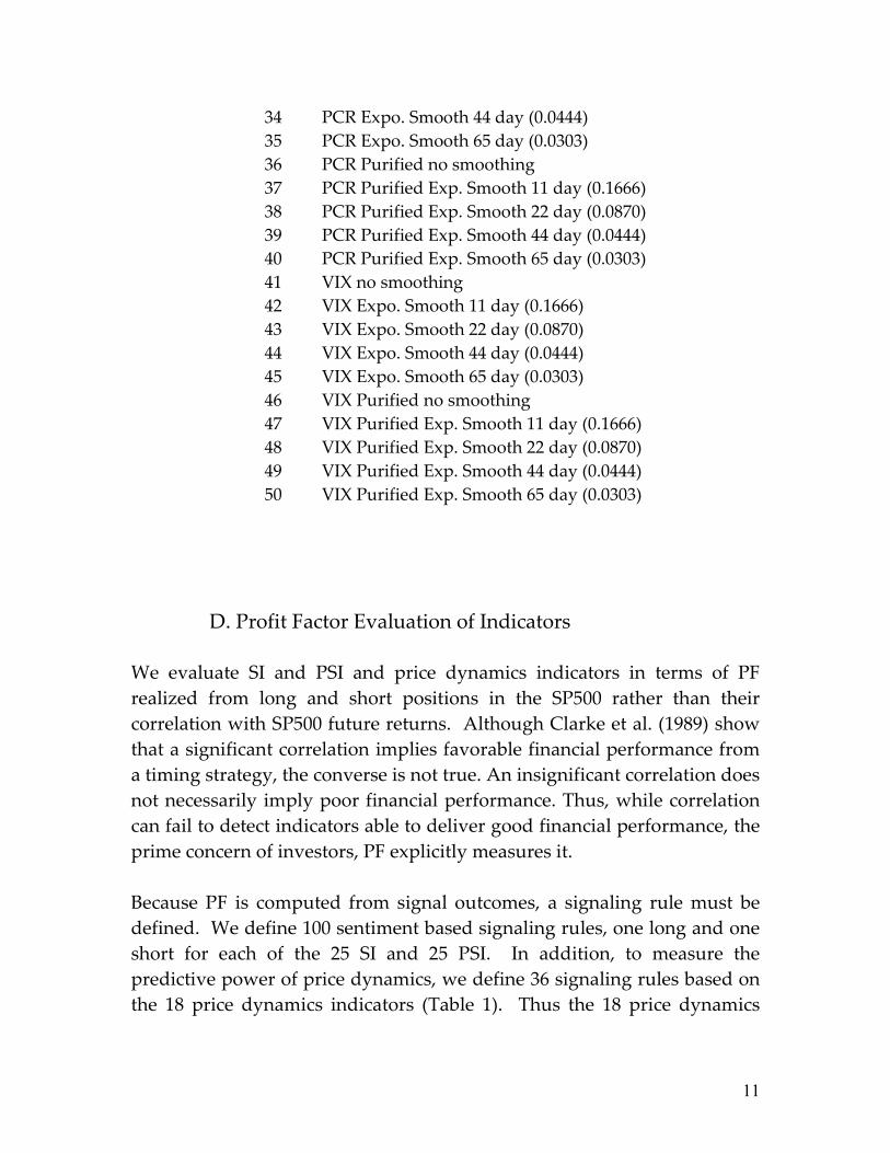
34 PCR Expo. Smooth 44 day (0.0444) 35 PCR Expo. Smooth 65 day (0.0303) 36 PCR Purified no smoothing 37 PCR Purified Exp. Smooth 11 day (0.1666) 38 PCR Purified Exp. Smooth 22 day (0.0870) 39 PCR Purified Exp. Smooth 44 day (0.0444) 40 PCR Purified Exp. Smooth 65 day (0.0303) 41 VIX no smoothing 42 VIX Expo. Smooth 11 day (0.1666) 43 VIX Expo. Smooth 22 day (0.0870) 44 VIX Expo. Smooth 44 day (0.0444) 45 VIX Expo. Smooth 65 day (0.0303) 46 VIX Purified no smoothing 47 VIX Purified Exp. Smooth 11 day (0.1666) 48 VIX Purified Exp. Smooth 22 day (0.0870) 49 VIX Purified Exp. Smooth 44 day (0.0444) 50 VIX Purified Exp. Smooth 65 day (0.0303)

D. Profit Factor Evaluation of Indicators We evaluate SI and PSI and price dynamics indicators in terms of PF realized from long and short positions in the SP500 rather than their correlation with SP500 future returns. Although Clarke et al. (1989) show that a significant correlation implies favorable financial performance from a timing strategy, the converse is not true. An insignificant correlation does not necessarily imply poor financial performance. Thus, while correlation can fail to detect indicators able to deliver good financial performance, the prime concern of investors, PF explicitly measures it. Because PF is computed from signal outcomes, a signaling rule must be defined. We define 100 sentiment based signaling rules, one long and one short for each of the 25 SI and 25 PSI. In addition, to measure the predictive power of price dynamics, we define 36 signaling rules based on the 18 price dynamics indicators (Table 1). Thus the 18 price dynamics

12

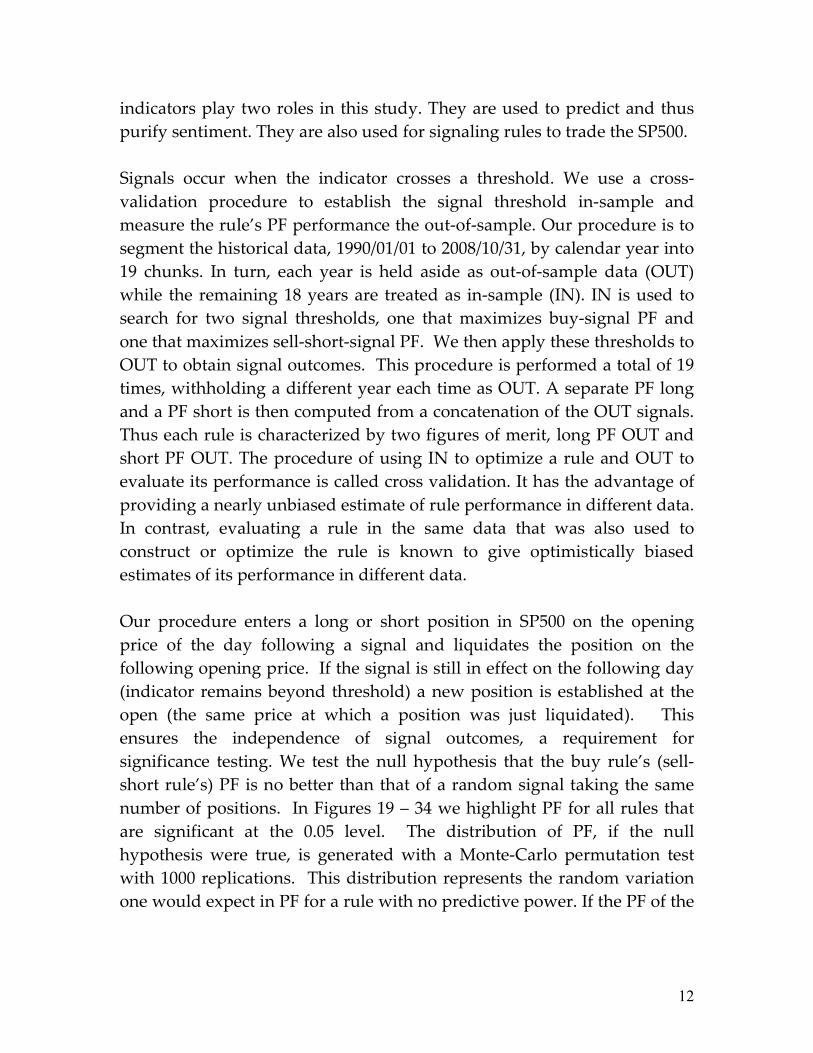
indicators play two roles in this study. They are used to predict and thus purify sentiment. They are also used for signaling rules to trade the SP500. Signals occur when the indicator crosses a threshold. We use a cross-validation procedure to establish the signal threshold in-sample and measure the rule’s PF performance the out-of-sample. Our procedure is to segment the historical data, 1990/01/01 to 2008/10/31, by calendar year into 19 chunks. In turn, each year is held aside as out-of-sample data (OUT) while the remaining 18 years are treated as in-sample (IN). IN is used to search for two signal thresholds, one that maximizes buy-signal PF and one that maximizes sell-short-signal PF. We then apply these thresholds to OUT to obtain signal outcomes. This procedure is performed a total of 19 times, withholding a different year each time as OUT. A separate PF long and a PF short is then computed from a concatenation of the OUT signals. Thus each rule is characterized by two figures of merit, long PF OUT and short PF OUT. The procedure of using IN to optimize a rule and OUT to evaluate its performance is called cross validation. It has the advantage of providing a nearly unbiased estimate of rule performance in different data. In contrast, evaluating a rule in the same data that was also used to construct or optimize the rule is known to give optimistically biased estimates of its performance in different data. Our procedure enters a long or short position in SP500 on the opening price of the day following a signal and liquidates the position on the following opening price. If the signal is still in effect on the following day (indicator remains beyond threshold) a new position is established at the open (the same price at which a position was just liquidated). This ensures the independence of signal outcomes, a requirement for significance testing. We test the null hypothesis that the buy rule’s (sell-short rule’s) PF is no better than that of a random signal taking the same number of positions. In Figures 19 – 34 we highlight PF for all rules that are significant at the 0.05 level. The distribution of PF, if the null hypothesis were true, is generated with a Monte-Carlo permutation test with 1000 replications. This distribution represents the random variation one would expect in PF for a rule with no predictive power. If the PF of the

13

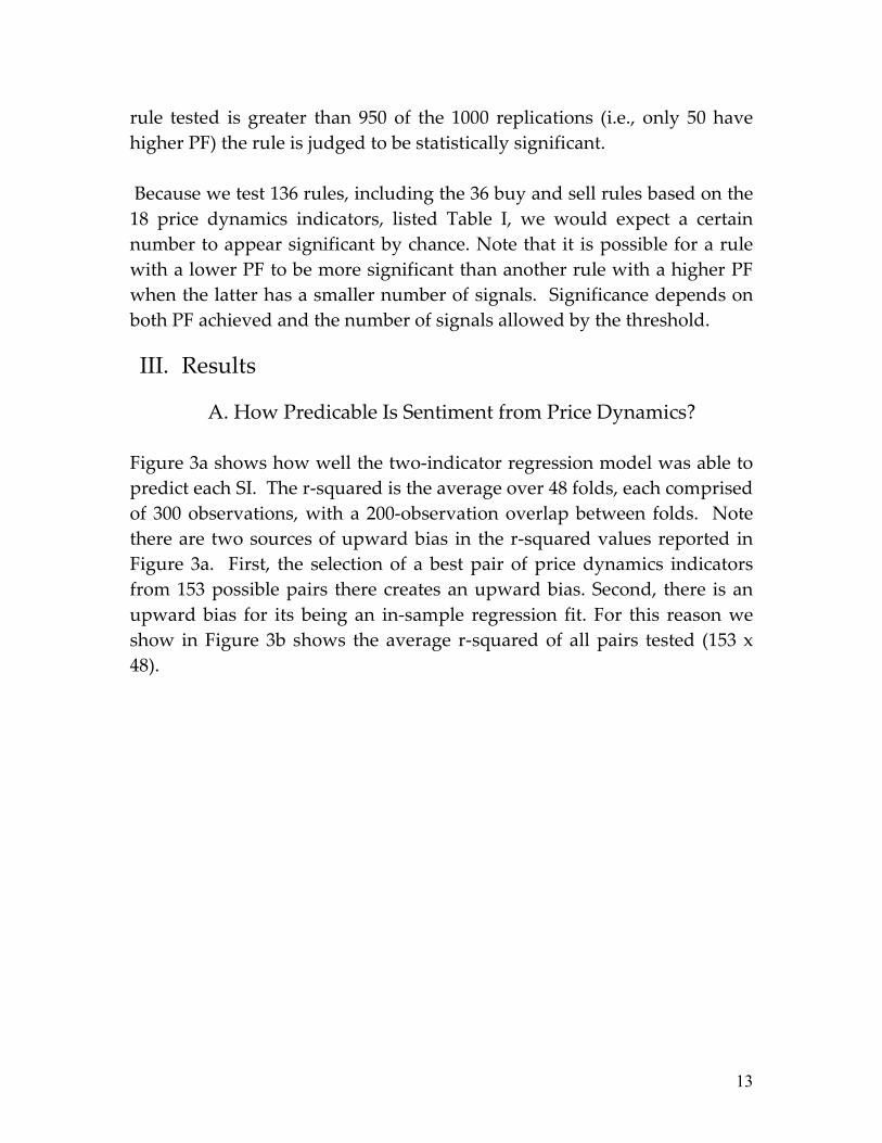
rule tested is greater than 950 of the 1000 replications (i.e., only 50 have higher PF) the rule is judged to be statistically significant. Because we test 136 rules, including the 36 buy and sell rules based on the 18 price dynamics indicators, listed Table I, we would expect a certain number to appear significant by chance. Note that it is possible for a rule with a lower PF to be more significant than another rule with a higher PF when the latter has a smaller number of signals. Significance depends on both PF achieved and the number of signals allowed by the threshold.

III. Results

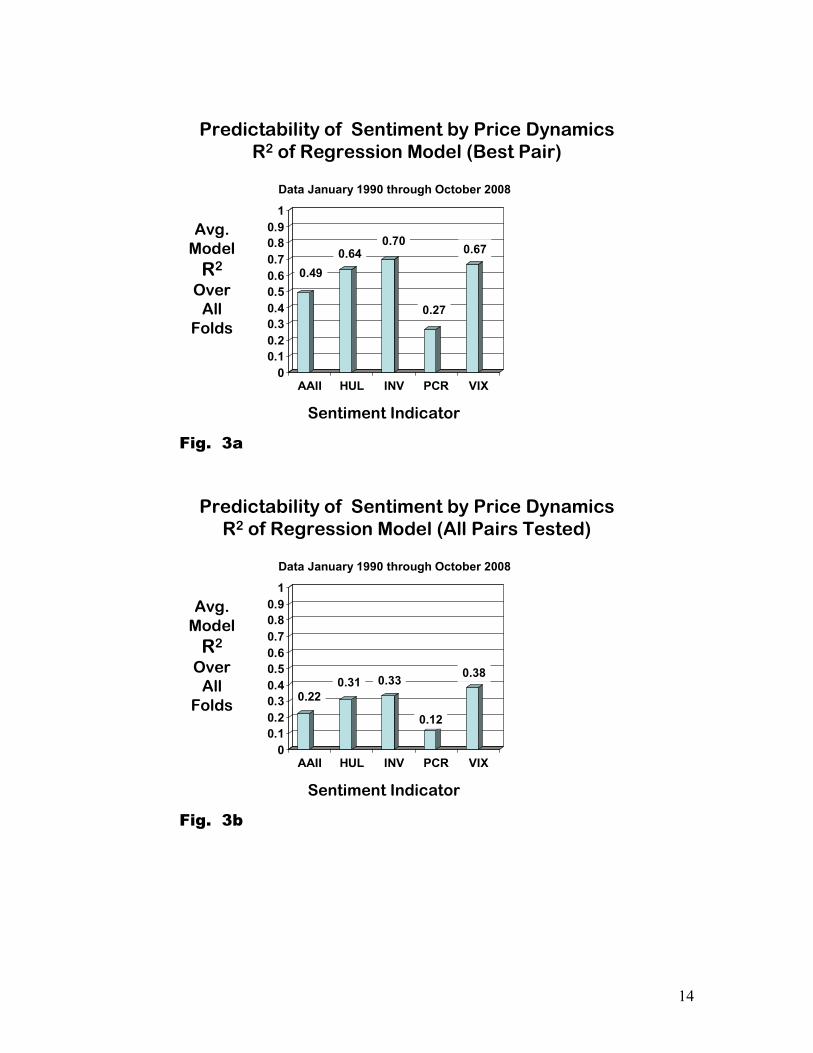
A. How Predicable Is Sentiment from Price Dynamics? Figure 3a shows how well the two-indicator regression model was able to predict each SI. The r-squared is the average over 48 folds, each comprised of 300 observations, with a 200-observation overlap between folds. Note there are two sources of upward bias in the r-squared values reported in Figure 3a. First, the selection of a best pair of price dynamics indicators from 153 possible pairs there creates an upward bias. Second, there is an upward bias for its being an in-sample regression fit. For this reason we show in Figure 3b shows the average r-squared of all pairs tested (153 x 48).

14

00.10.20.30.40.50.60.70.80.9

1

AAII HUL INV PCR VIX

EastWest

Predictability of Sentiment by Price Dynamics R2 of Regression Model (Best Pair)

Sentiment Indicator

Avg.Model

R2

OverAll

Folds

0.490.64

0.700.67

0.27

Fig. 3a

Data January 1990 through October 2008

00.10.20.30.40.50.60.70.80.9

1

AAII HUL INV PCR VIX

EastWest

Predictability of Sentiment by Price Dynamics R2 of Regression Model (All Pairs Tested)

Sentiment Indicator

0.220.31 0.33 0.38

0.12

Fig. 3b

Data January 1990 through October 2008

Avg.Model

R2

OverAll

Folds

15

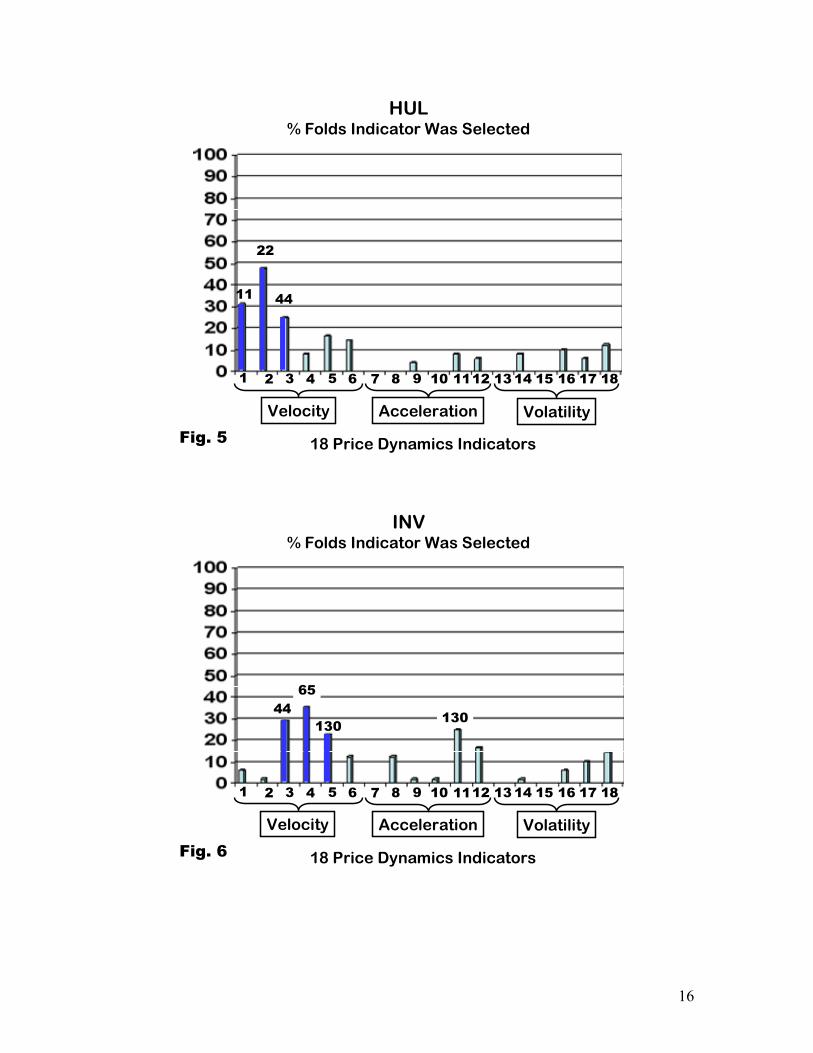
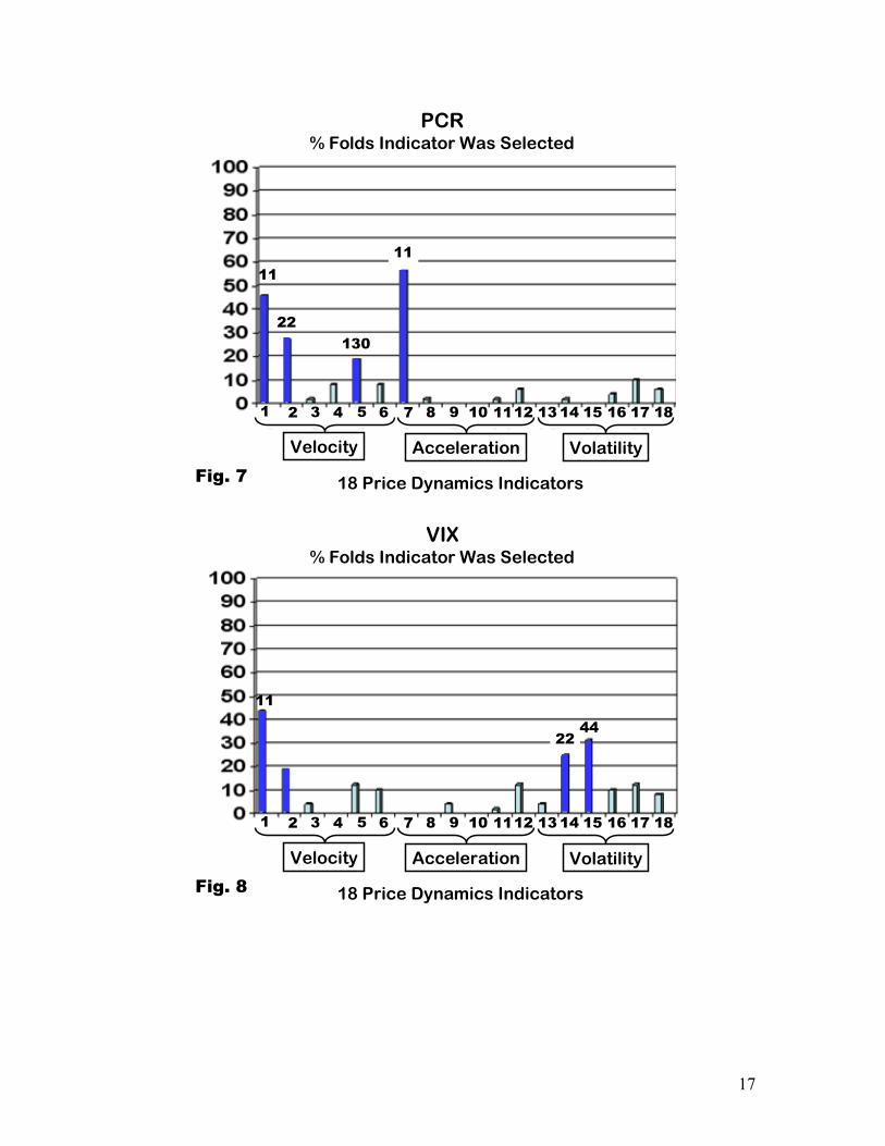
B. Relative Importance of 18 Price Dynamics Indicators in Predicting Sentiment

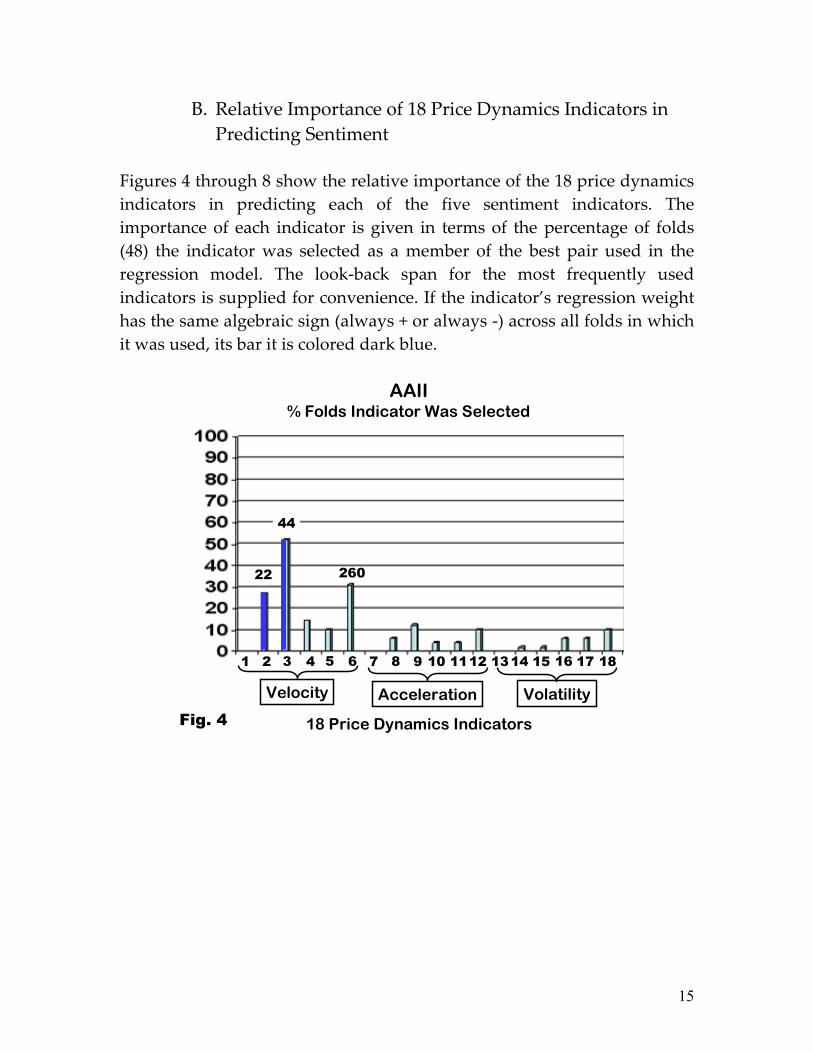
Figures 4 through 8 show the relative importance of the 18 price dynamics indicators in predicting each of the five sentiment indicators. The importance of each indicator is given in terms of the percentage of folds (48) the indicator was selected as a member of the best pair used in the regression model. The look-back span for the most frequently used indicators is supplied for convenience. If the indicator’s regression weight has the same algebraic sign (always + or always -) across all folds in which it was used, its bar it is colored dark blue.

18 Price Dynamics Indicators

44

22

4 6 8 9 13101 2 3 5 7 1411 15 1716 18124 86

Velocity Acceleration Volatility

Fig. 4

260

AAII% Folds Indicator Was Selected

16


1 9 11 13 15 1710


16 182 3 4 5 7 8 12 146

22

11

Fig. 5

HUL% Folds Indicator Was Selected

44

1 9 10 16 182 3 4 5 7 8 12 146 11 13 15 17


44

18 Price Dynamics IndicatorsFig. 6

65

130 130

INV% Folds Indicator Was Selected

17



11

1 9 102 3 4 5 7 8 126 13 15 171411 16 18

Fig. 7

11

22130

PCR% Folds Indicator Was Selected

1 9 10 16 182 3 4 5 7 8 12 146 11 13 15 17


11

18 Price Dynamics IndicatorsFig. 8

2244

VIX% Folds Indicator Was Selected

18

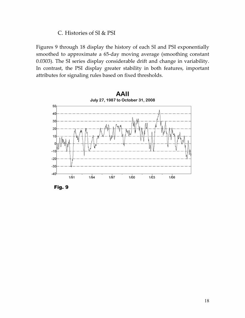
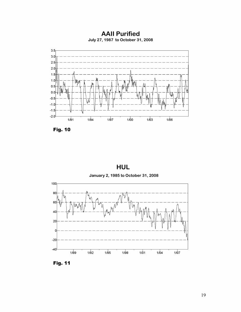
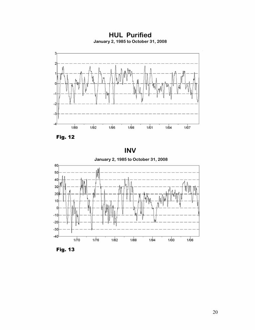
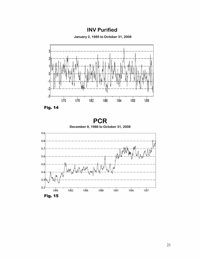
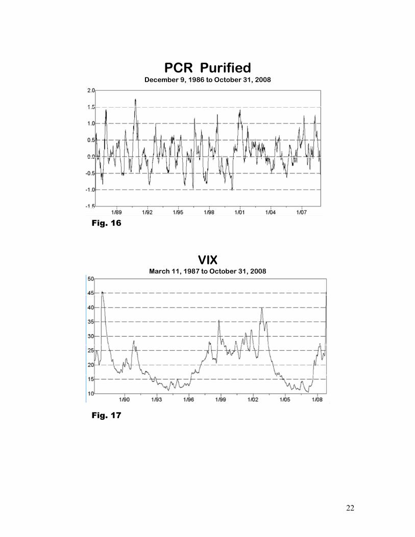
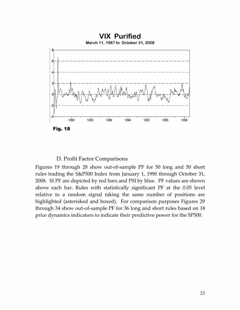
C. Histories of SI & PSI Figures 9 through 18 display the history of each SI and PSI exponentially smoothed to approximate a 65-day moving average (smoothing constant 0.0303). The SI series display considerable drift and change in variability. In contrast, the PSI display greater stability in both features, important attributes for signaling rules based on fixed thresholds.

AAII July 27, 1987 to October 31, 2008

Fig. 9

19

Fig. 10

AAII Purified July 27, 1987 to October 31, 2008

Fig. 11

HULJanuary 2, 1985 to October 31, 2008

20

Fig. 12

HUL PurifiedJanuary 2, 1985 to October 31, 2008

Fig. 13

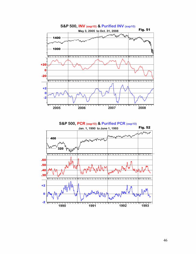
INVJanuary 2, 1985 to October 31, 2008

21

Fig. 14

INV PurifiedJanuary 2, 1985 to October 31, 2008

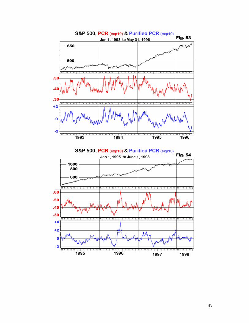
PCRDecember 9, 1986 to October 31, 2008

Fig. 15

22

Fig. 16

PCR PurifiedDecember 9, 1986 to October 31, 2008

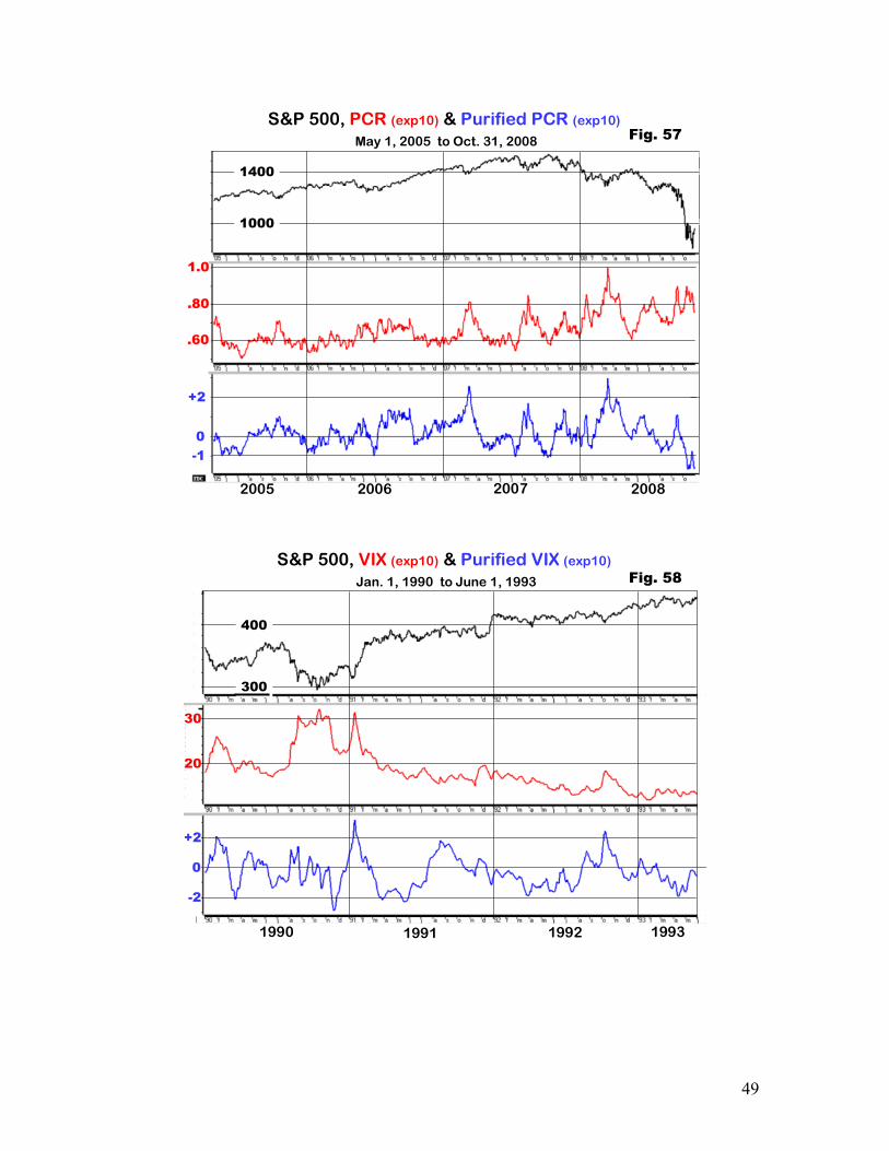
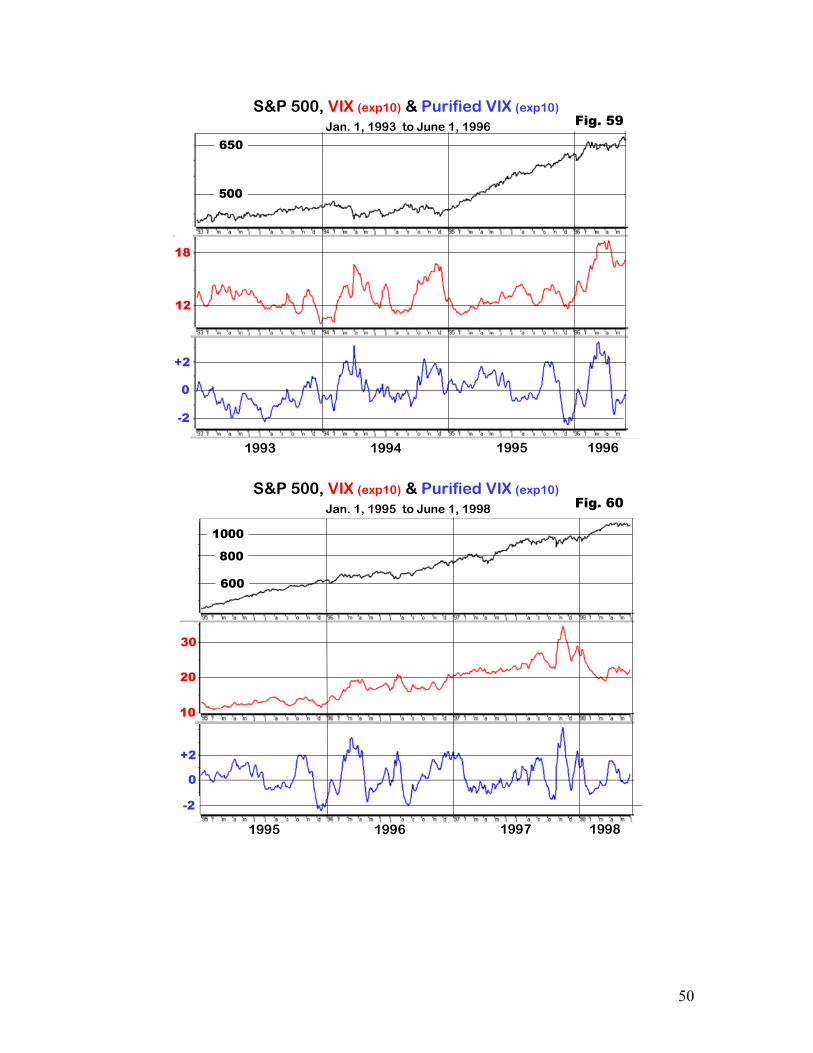
VIXMarch 11, 1987 to October 31, 2008

Fig. 17

23

Fig. 18

VIX PurifiedMarch 11, 1987 to October 31, 2008

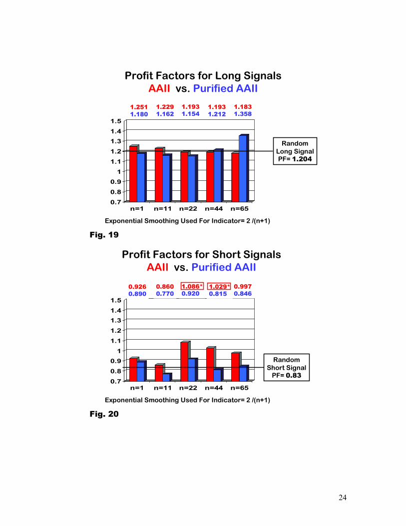
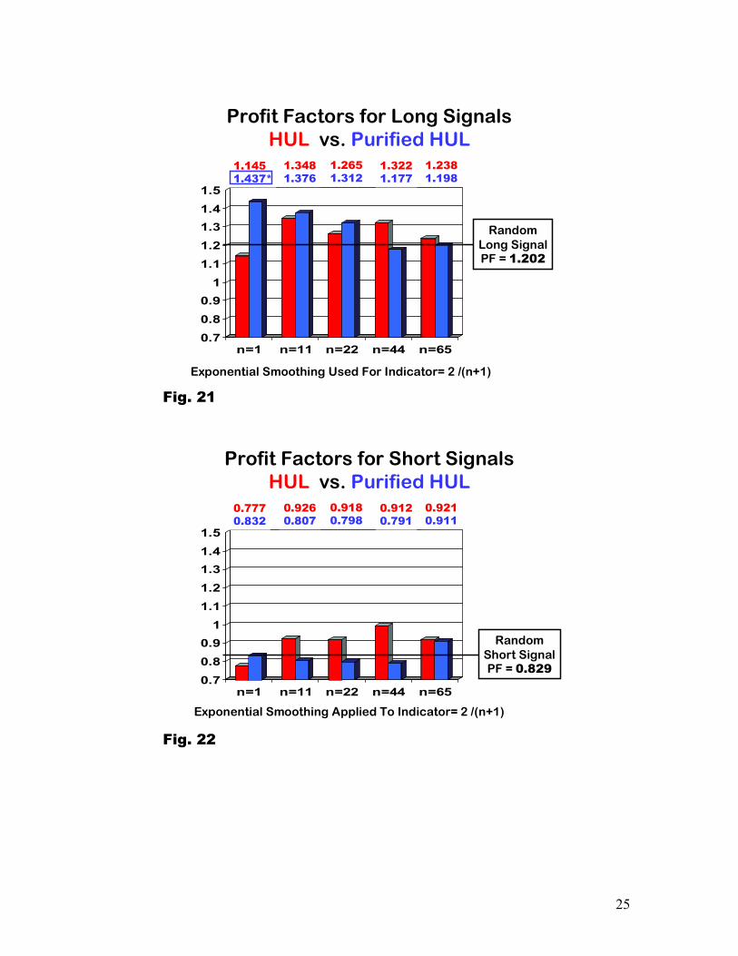
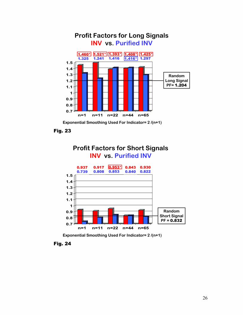
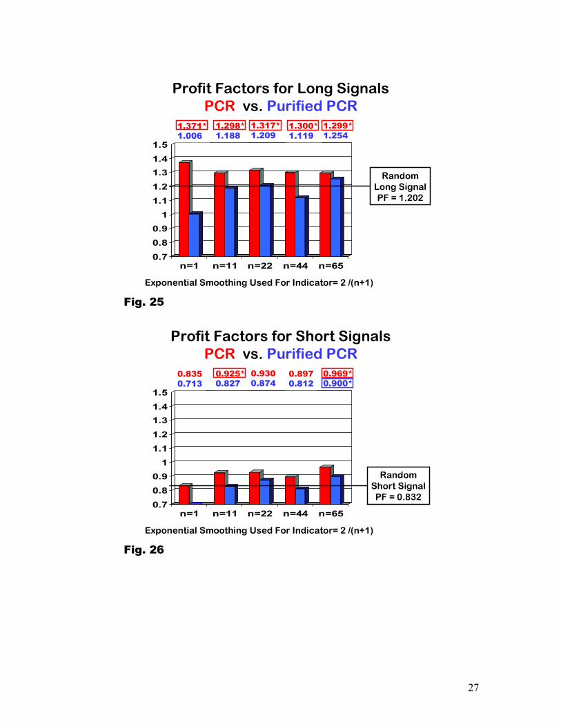
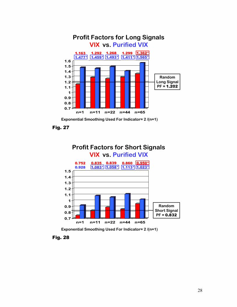
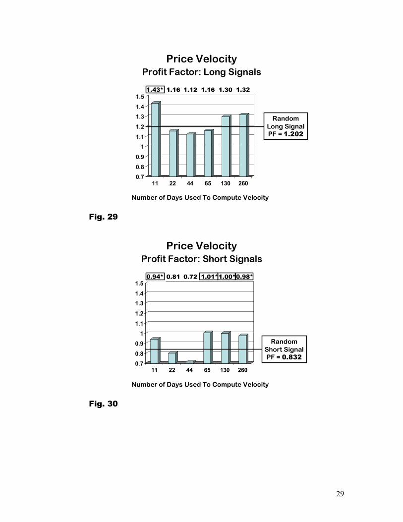
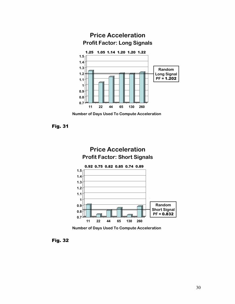
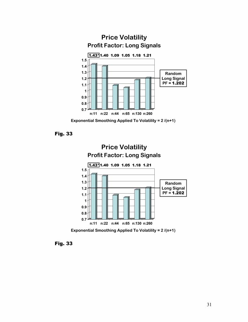
D. Profit Factor Comparisons Figures 19 through 28 show out-of-sample PF for 50 long and 50 short rules trading the S&P500 Index from January 1, 1990 through October 31, 2008. SI PF are depicted by red bars and PSI by blue. PF values are shown above each bar. Rules with statistically significant PF at the 0.05 level relative to a random signal taking the same number of positions are highlighted (asterisked and boxed). For comparison purposes Figures 29 through 34 show out-of-sample PF for 36 long and short rules based on 18 price dynamics indicators to indicate their predictive power for the SP500.

24

Profit Factors for Long SignalsAAII vs. Purified AAII

0.70.80.9

11.11.21.31.41.5

n=1 n=11 n=22 n=44 n=65

OrdinaryPurified

RandomLong SignalPF= 1.204

1.2511.180

1.2291.162

1.1931.154

1.1931.212

1.1831.358

Exponential Smoothing Used For Indicator= 2 /(n+1)

Fig. 19

Profit Factors for Short SignalsAAII vs. Purified AAII

0.70.80.9

11.11.21.31.41.5

n=1 n=11 n=22 n=44 n=65

OrdinaryPurified

0.9260.890

0.8600.770

1.086*0.920

1.029*0.815

0.9970.846

RandomShort Signal

PF= 0.83


Fig. 20

25

Profit Factors for Long SignalsHUL vs. Purified HUL

0.70.80.9

11.11.21.31.41.5

n=1 n=11 n=22 n=44 n=65

OrdinaryPurified

1.1451.437*

1.3481.376

1.2651.312

1.3221.177

1.2381.198

RandomLong SignalPF = 1.202


Fig. 21

Profit Factors for Short SignalsHUL vs. Purified HUL

0.70.80.9

11.11.21.31.41.5

n=1 n=11 n=22 n=44 n=65

OrdinaryPurified

Exponential Smoothing Applied To Indicator= 2 /(n+1)

0.7770.832

0.9260.807

0.9180.798

0.9120.791

0.9210.911

RandomShort SignalPF = 0.829

Fig. 22

26

Profit Factors for Long SignalsINV vs. Purified INV

0.70.80.9

11.11.21.31.41.5

n=1 n=11 n=22 n=44 n=65

OrdinaryPurified

RandomLong SignalPF= 1.204

1.460*1.325

1.521*1.241

1.393*1.416

1.408*1.416*

1.425*1.297


Fig. 23

Profit Factors for Short SignalsINV vs. Purified INV

0.70.80.9

11.11.21.31.41.5

n=1 n=11 n=22 n=44 n=65

OrdinaryPurified

0.9370.739

0.9170.808

0.953*0.853

0.8430.840

0.9300.822



Fig. 24

27

Profit Factors for Long SignalsPCR vs. Purified PCR

0.70.80.9

11.11.21.31.41.5

n=1 n=11 n=22 n=44 n=65

OrdinaryPurified


1.371*1.006

1.298*1.188

1.317*1.209

1.300*1.119

1.299*1.254


Fig. 25

Profit Factors for Short SignalsPCR vs. Purified PCR

0.70.80.9

11.11.21.31.41.5

n=1 n=11 n=22 n=44 n=65

OrdinaryPurified


0.8350.713

0.925*0.827

0.9300.874

0.8970.812

0.969*0.900*


Fig. 26

28

Profit Factors for Long SignalsVIX vs. Purified VIX

0.70.80.9

11.11.21.31.41.51.6

n=1 n=11 n=22 n=44 n=65

OrdinaryPurified

1.1631.477*

1.2921.459*

1.2681.493*

1.2991.411*

1.362*1.565*



Fig. 27

Profit Factors for Short SignalsVIX vs. Purified VIX

0.70.80.9

11.11.21.31.41.5

n=1 n=11 n=22 n=44 n=65

OrdinaryPurified

0.7520.928

0.8351.083*

0.8391.058*

0.8601.113*

0.950*1.023*



Fig. 28

29

0.70.80.9

11.11.21.31.41.5

11 22 44 65 130 260

East


1.43* 1.16

Number of Days Used To Compute Velocity

Price Velocity Profit Factor: Long Signals

1.12 1.16 1.30 1.32

Fig. 29

0.70.80.9

11.11.21.31.41.5

11 22 44 65 130 260

East


Price Velocity Profit Factor: Short Signals

0.94* 0.81 0.72 1.01*1.00*0.98*

Number of Days Used To Compute Velocity

Fig. 30

30

0.70.80.9

11.11.21.31.41.5

11 22 44 65 130 260

East


Price Acceleration Profit Factor: Long Signals

1.25 1.05 1.14 1.20 1.20 1.22

Number of Days Used To Compute Acceleration

Fig. 31

0.70.80.9

11.11.21.31.41.5

11 22 44 65 130 260

East

Price Acceleration Profit Factor: Short Signals

0.92 0.75 0.82 0.85 0.74 0.89

Number of Days Used To Compute Acceleration


Fig. 32

31

0.70.80.9

11.11.21.31.41.5

n:11 n:22 n:44 n:65 n:130 n:260

East


Exponential Smoothing Applied To Volatility = 2 /(n+1)

Price Volatility Profit Factor: Long Signals

1.43*1.40 1.09 1.05 1.18 1.21

Fig. 33

0.70.80.9

11.11.21.31.41.5

n:11 n:22 n:44 n:65 n:130 n:260

East



Price Volatility Profit Factor: Long Signals

1.43*1.40 1.09 1.05 1.18 1.21

Fig. 33

32

0.70.80.9

11.11.21.31.41.5

n:11 n:22 n:44 n:65 n:130 n:260

East


Price Volatility Profit Factor: Short Signals

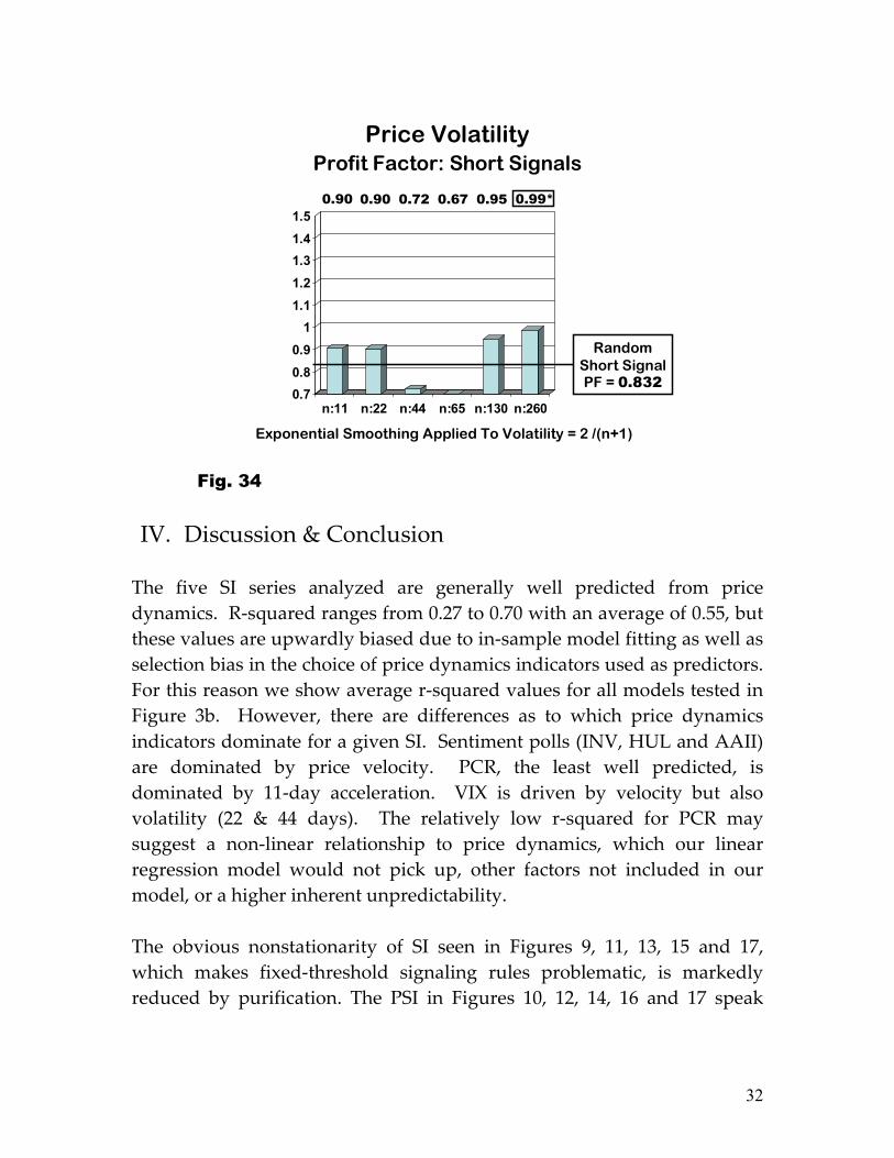
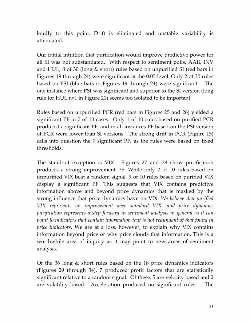
0.90 0.90 0.72 0.67 0.95 0.99*


Fig. 34

IV. Discussion & Conclusion The five SI series analyzed are generally well predicted from price dynamics. R-squared ranges from 0.27 to 0.70 with an average of 0.55, but these values are upwardly biased due to in-sample model fitting as well as selection bias in the choice of price dynamics indicators used as predictors. For this reason we show average r-squared values for all models tested in Figure 3b. However, there are differences as to which price dynamics indicators dominate for a given SI. Sentiment polls (INV, HUL and AAII) are dominated by price velocity. PCR, the least well predicted, is dominated by 11-day acceleration. VIX is driven by velocity but also volatility (22 & 44 days). The relatively low r-squared for PCR may suggest a non-linear relationship to price dynamics, which our linear regression model would not pick up, other factors not included in our model, or a higher inherent unpredictability. The obvious nonstationarity of SI seen in Figures 9, 11, 13, 15 and 17, which makes fixed-threshold signaling rules problematic, is markedly reduced by purification. The PSI in Figures 10, 12, 14, 16 and 17 speak

33

loudly to this point. Drift is eliminated and unstable variability is attenuated. Our initial intuition that purification would improve predictive power for all SI was not substantiated. With respect to sentiment polls, AAII, INV and HUL, 8 of 30 (long & short) rules based on unpurified SI (red bars in Figures 19 through 24) were significant at the 0.05 level. Only 2 of 30 rules based on PSI (blue bars in Figures 19 through 24) were significant. The one instance where PSI was significant and superior to the SI version (long rule for HUL n=1 in Figure 21) seems too isolated to be important. Rules based on unpurified PCR (red bars in Figures 25 and 26) yielded a significant PF in 7 of 10 cases. Only 1 of 10 rules based on purified PCR produced a significant PF, and in all instances PF based on the PSI version of PCR were lower than SI versions. The strong drift in PCR (Figure 15) calls into question the 7 significant PF, as the rules were based on fixed thresholds. The standout exception is VIX. Figures 27 and 28 show purification produces a strong improvement PF. While only 2 of 10 rules based on unpurified VIX beat a random signal, 9 of 10 rules based on purified VIX display a significant PF. This suggests that VIX contains predictive information above and beyond price dynamics that is masked by the strong influence that price dynamics have on VIX. We believe that purified VIX represents an improvement over standard VIX, and price dynamics purification represents a step forward in sentiment analysis in general as it can point to indicators that contain information that is not redundant of that found in price indicators. We are at a loss, however, to explain why VIX contains information beyond price or why price clouds that information. This is a worthwhile area of inquiry as it may point to new areas of sentiment analysis. Of the 36 long & short rules based on the 18 price dynamics indicators (Figures 29 through 34), 7 produced profit factors that are statistically significant relative to a random signal. Of these, 5 are velocity based and 2 are volatility based. Acceleration produced no significant rules. The

34

predictive power in velocity and the strong impact of velocity on sentiment polls (AAII, INV & HUL) suggests that the predictive power residing in the unpurified form may largely derive from the predictive power of velocity. In other words, the polls are proxies for price velocity. A strong motivation for utilizing SI is to obtain predictive information that is independent of and accretive to that found in price-based indicators. Our study of suggests that AAII, INV, HUL and PCR add minimal value once price indicators have been utilized. This is most problematic for analysts who use subjective judgment to combine price indicators with unpurified sentiment indicators. This double counting could result in price being given excessive weight. Those using a statistical model derived with automated indicator selection do not face this issue as redundant indicators are not likely to be included in the model.

35

References

Brown, Gregory, W. and Cliff, Michael T. (2004), “Investor sentiment and the near-term stock market”, Journal of Empirical Finance, vol 11, no.1, (January):1-27

Clark, R.G., Fitzgerald, M.T, Berant, P. and Statman, M. (1989), “Market Timing with Imperfect Information.”, Financial Analysts Journal, vol. 45, no. 6, (November/December): 27-36

Clark, R.G., and Statman, Meir (1998), “Bullish or Bearish?”, Financial Analysts Journal, (May/June), 63-72

De Bondt, Werner, (1993), “Betting on Trends: Intuitive Forecasts of Financial Risk and Return”, International Journal of Forecasting, vol. 9, no.3, (November): 355-371

Fisher, Kenneth L. and Statman, Meir (2000), “Investor sentiment and stock returns, Financial Analysts Journal, Vol. 56, no. 2. (Mar/April): 16-23

Fosback, Norman, G., (1976), Stock Market Logic: A Sophisticated Approach to Profits on Wall Street, Dearborn Financial Publishing, Inc., The book is no longer in print.

Goepfert, Jason, “Mutual Fund Cash Reserves, the Risk-Free Rate and Stock Market Performance, MTA Journal, no. 62 (Summer-Fall 2004):12-17

Hayes, Timothy, (1994), “Using Market Sentiment in One Market to Call Prices in Another”,MTA Journal, no. 44, (Winter 1994-Spring 1995):10-25

Hayes, Timothy, (2001), The Research Driven Investor, McGraw-Hill, New York

Jacobs, Bruce and Levy Kenneth, (2000), Equity Management: Quantitative Analysis for Stock Selection, McGraw-Hill, New York

Merrill, Arthur, (1982)“ DFE Deviation From Expected (Relative Strength Corrected for Beta), MTA Journal, no. 14, (August): 21-28

36

Simon, David P. and Wiggens III, Roy A., (2001) “S&P futures returns and contrary sentiment indicators”, The Journal of Futures Markets, Vol.21, no.5

Solt, Machael E., and Statman, Meir (1998), “How Useful is the Sentiment Index.?”, Financial Analysts Journal, vol. 44, no.5, (September/October):44-55

Stonecypher, Lance, (1988) “Liquidity Indicators – Still Valuable Market Timing Tools, MTA Journal, no. 29 (February):15-23

Wang, Yaw-Huei and Kewwani, Aneel and Taylor, Stephan J., (2006)“The relationships between sentiment, returns and volatility”, International Journal of Forecasting vol. 22, no. 1 (Jan-March).

37

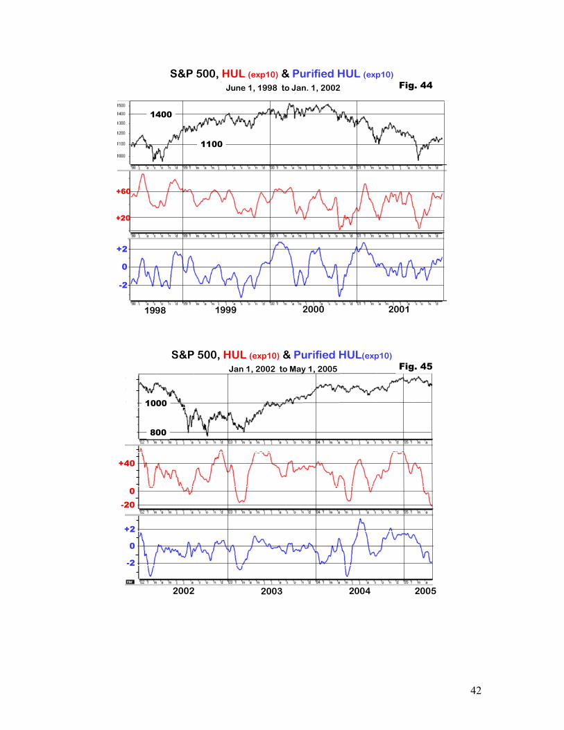
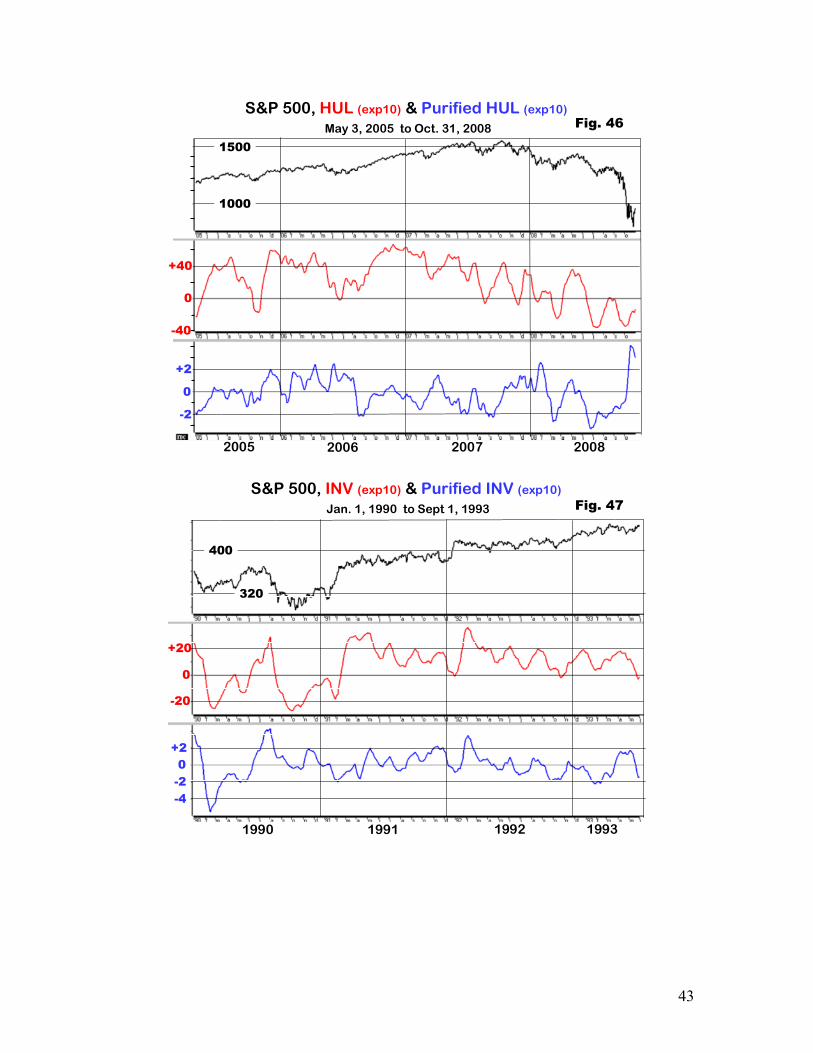
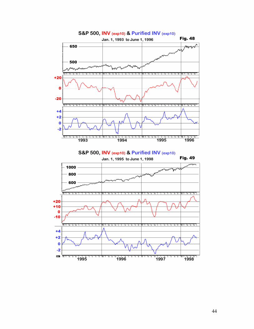
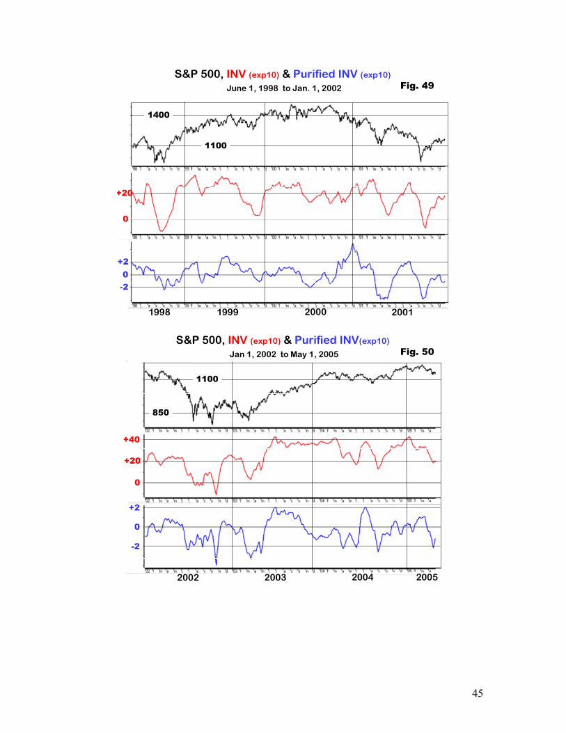
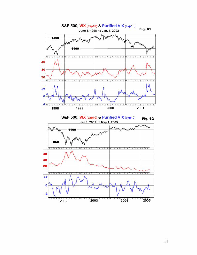
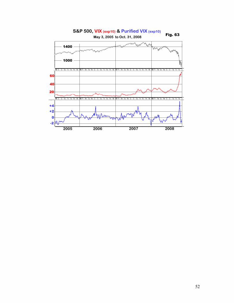
Appendix 1

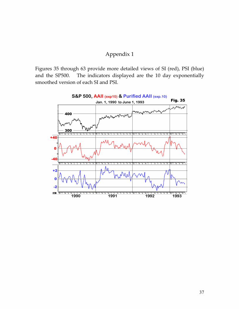
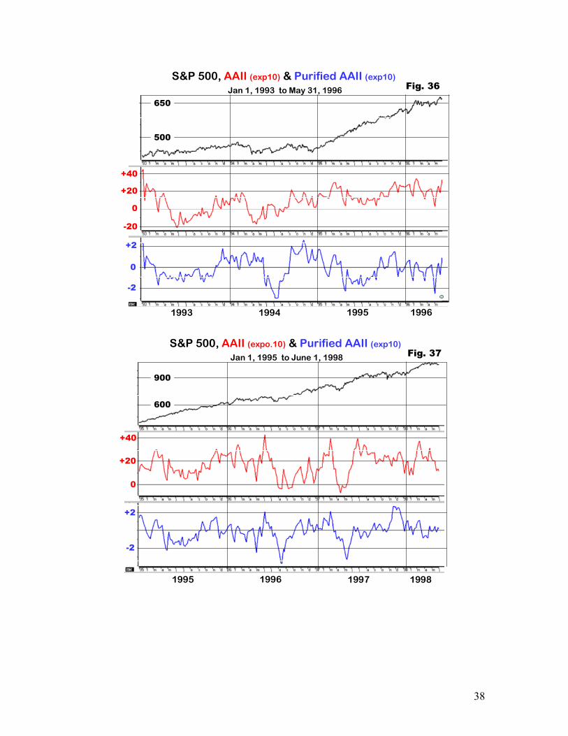
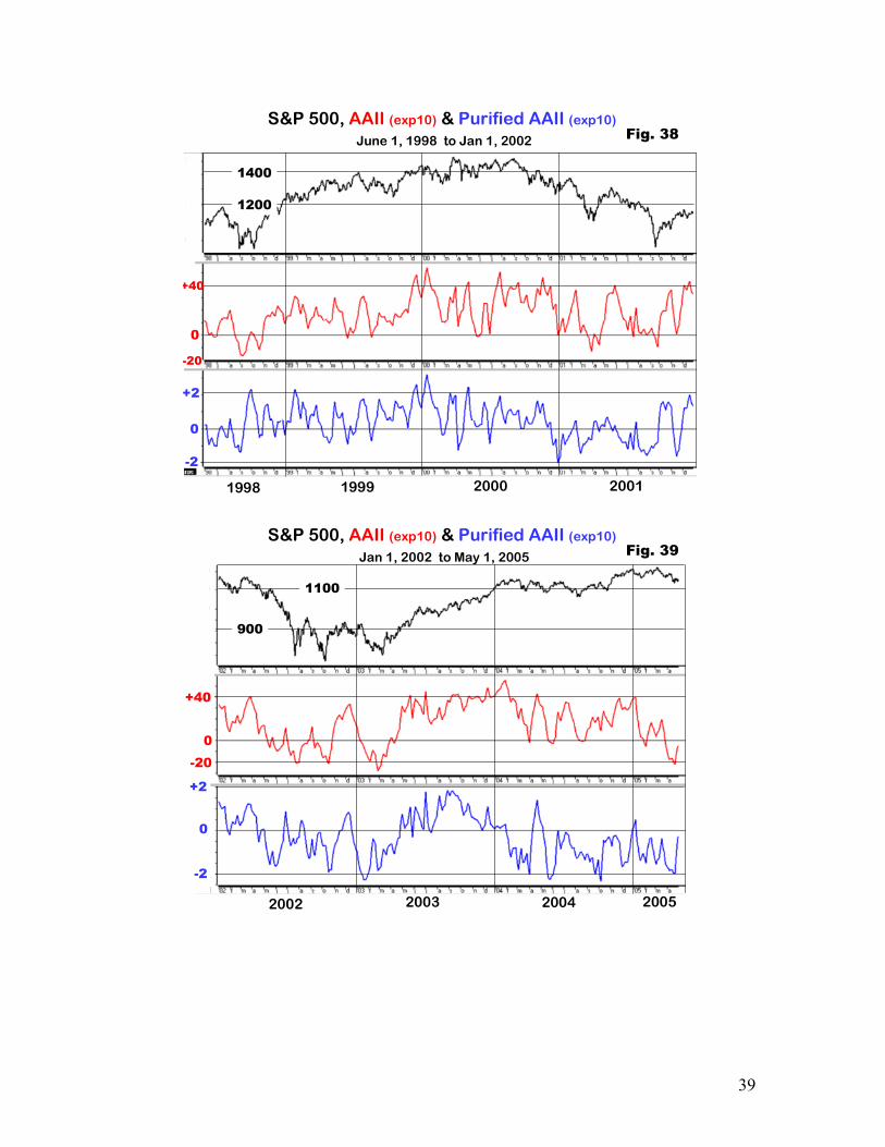
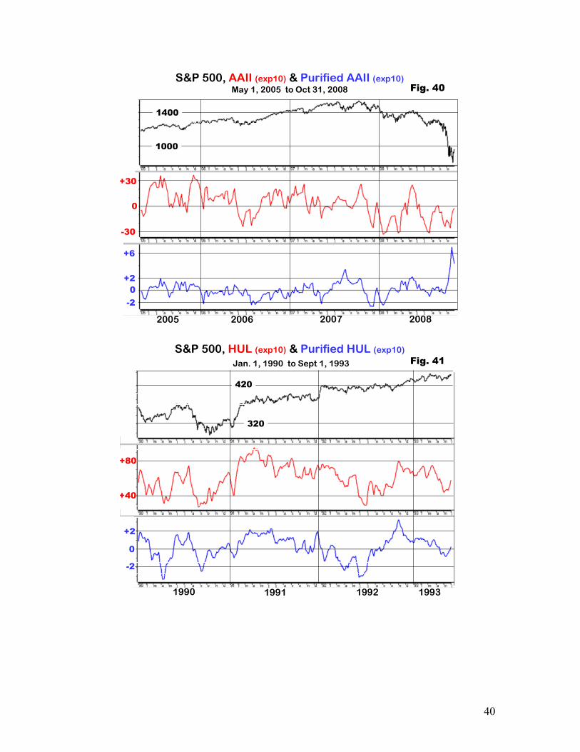
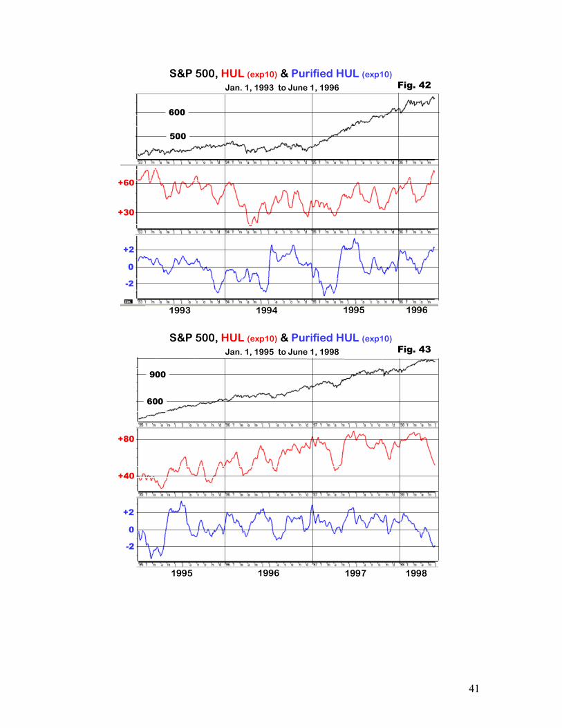
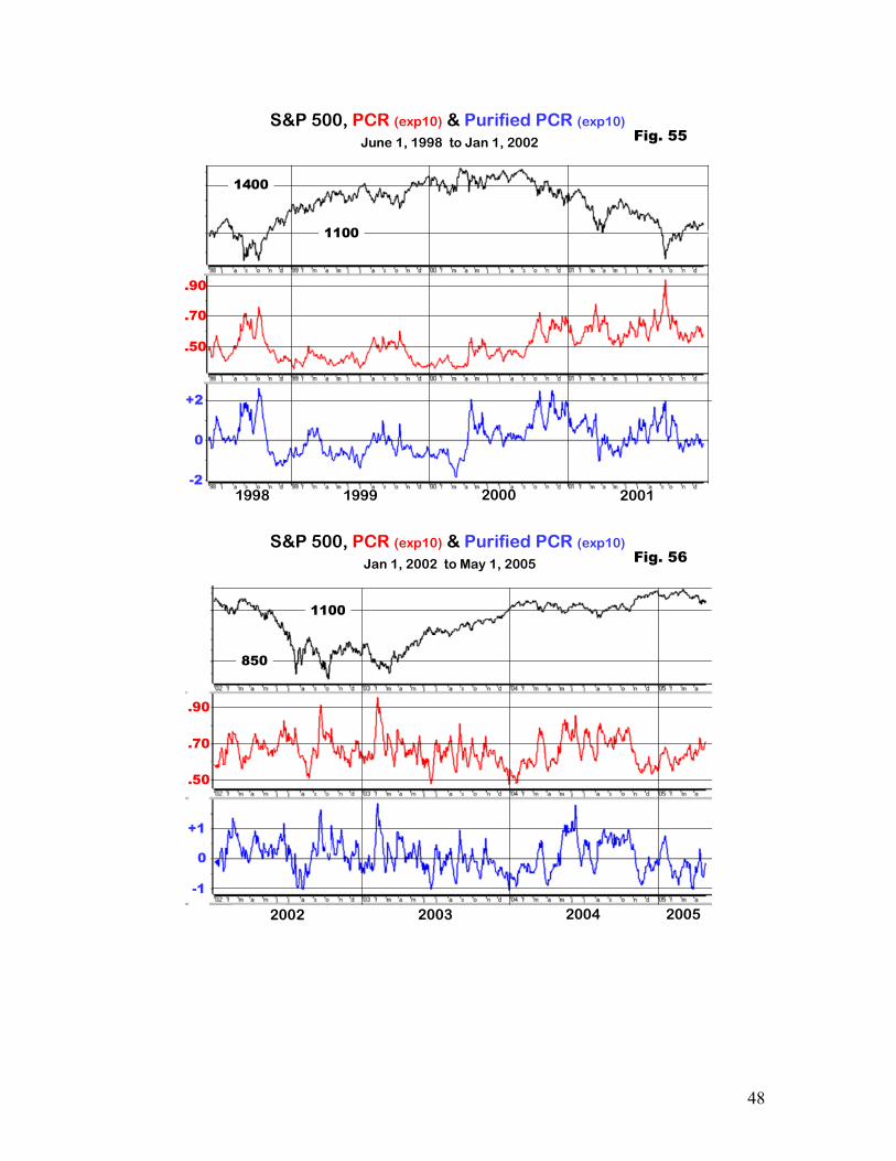
Figures 35 through 63 provide more detailed views of SI (red), PSI (blue) and the SP500. The indicators displayed are the 10 day exponentially smoothed version of each SI and PSI.

1991 1992 19931990

+2

0

-2

+40

-40

0

Fig. 35

400

300

S&P 500, AAII (exp10) & Purified AAII (exp.10)

Jan. 1, 1990 to June 1, 1993

38

S&P 500, AAII (exp10) & Purified AAII (exp10)

Jan 1, 1993 to May 31, 1996 Fig. 36

+2

-2

0

+40

0

-20

500

650

+20

1994 1995 19961993

Fig. 37

+2

-2

+40

+20

0

600

900

S&P 500, AAII (expo.10) & Purified AAII (exp10)

Jan 1, 1995 to June 1, 1998

1996 1997 19981995

39


June 1, 1998 to Jan 1, 2002 Fig. 38

1400

1200

-20

0

+40

+2

-2

0

1999 2000 20011998


Jan 1, 2002 to May 1, 2005 Fig. 39

-2

0

+2

2003 2004 20052002

0-20

+40

1100

900

40

S&P 500, AAII (exp10) & Purified AAII (exp10)May 1, 2005 to Oct 31, 2008

-20

+2

+6

1400

1000

+30

-30

0

2006 2007 20082005

Fig. 40

S&P 500, HUL (exp10) & Purified HUL (exp10)

Jan. 1, 1990 to Sept 1, 1993

1991 1992 19931990

Fig. 41

420

320

+2

0

-2

+40

+80

41


Jan. 1, 1993 to June 1, 1996 Fig. 42

1994 1995 19961993

+60

+30

600

500

+2

0

-2


Jan. 1, 1995 to June 1, 1998 Fig. 43

1996 1997 19981995

600

900

+2

0

-2

+80

+40

42


June 1, 1998 to Jan. 1, 2002 Fig. 44

1999 2000 20011998

0

+2

-2

+20

+60

1100

1400

S&P 500, HUL (exp10) & Purified HUL(exp10)

Jan 1, 2002 to May 1, 2005

-200

+40

0

+2

-2

2003 2004 20052002

1000

800

Fig. 45

43


May 3, 2005 to Oct. 31, 2008

2006 2007 20082005

1500

1000

+40

0

-40

0

+2

-2

Fig. 46

S&P 500, INV (exp10) & Purified INV (exp10)

Jan. 1, 1990 to Sept 1, 1993

1991 1992 19931990

Fig. 47

-20

+2

+20

-20

0

400

320

-4

44


Jan. 1, 1993 to June 1, 1996 Fig. 48

1994 1995 19961993

-20

+2+4

-20

+20

0

500

650


Jan. 1, 1995 to June 1, 1998 Fig. 49

1996 1997 19981995

+4+20-2

-100

+20

1000

800

600

+10

45


June 1, 1998 to Jan. 1, 2002 Fig. 49

1999 2000 20011998

0+2

-2

0

+20

1100

1400

S&P 500, INV (exp10) & Purified INV(exp10)

Jan 1, 2002 to May 1, 2005 Fig. 50

2003 2004 20052002

0

+20

+40

0

+2

-2

850

1100

46


May 3, 2005 to Oct. 31, 2008

2006 2007 20082005

1400

1000

0

+20

-20

0+2

-2

Fig. 51

S&P 500, PCR (exp10) & Purified PCR (exp10)

Jan. 1, 1990 to June 1, 1993

1991 1992 19931990

+2

0

-2

.30

.40

.50

.60

400

Fig. 52

320

47


Jan 1, 1993 to May 31, 1996

1994 1995 19961993

Fig. 53

500

650

.30

.40

.50

+2

0

-2


Jan 1, 1995 to June 1, 1998

1996 1997 19981995

Fig. 54

+4

+2

0

-2

.30

.40

.50

.60

1000800

600

48


June 1, 1998 to Jan 1, 2002

.50

.70

.90

+2

0

-2

1100

1400

Fig. 55

1999 2000 20011998


Jan 1, 2002 to May 1, 2005 Fig. 56

2003 2004 20052002

850

1100

.50

.70

.90

0

+1

-1

49


May 1, 2005 to Oct. 31, 2008 Fig. 57

2006 2007 20082005

1.0

.80

.60

1000

1400

-10

+2

S&P 500, VIX (exp10) & Purified VIX (exp10)

Jan. 1, 1990 to June 1, 1993

1991 1992 19931990

400

300

30

20

+2

-2

0

Fig. 58

50


Jan. 1, 1993 to June 1, 1996 Fig. 59

-2

0

+2

12

18

1994 1995 19961993

500

650


Jan. 1, 1995 to June 1, 1998

1000

800

600

1996 1997 19981995

+2

-2

0

20

30

10

Fig. 60

51


June 1, 1998 to Jan. 1, 2002

1999 2000 20011998

-2

0

+2

20

30

40

Fig. 61

1100

1400


Jan 1, 2002 to May 1, 2005

+2

-2

0

2003 2004 20052002

20

40

30

Fig. 62

850

1100

52


May 3, 2005 to Oct. 31, 2008

2006 2007 20082005

40

60

20

+2

-20

+4

Fig. 63

1000

1400

Date post:	20-May-2018
Category:	Documents
Upload:	lekiet
View:	224 times
Download:	1 times

Purified Sentiment Indicators for the Stock Market...

Documents