+ All Categories
Home > Documents > Pursuing Collective Synchrony in Teams: A Regime-Switching ...

Pursuing Collective Synchrony in Teams: A Regime-Switching ...

Date post: 06-Apr-2022
Category:
Upload: others
View: 2 times
Download: 0 times
Share this document with a friend
43
University of Rhode Island University of Rhode Island DigitalCommons@URI DigitalCommons@URI Psychology Faculty Publications Psychology 2021 Pursuing Collective Synchrony in Teams: A Regime-Switching Pursuing Collective Synchrony in Teams: A Regime-Switching Dynamic Factor Model of Speed Similarity in Soccer Dynamic Factor Model of Speed Similarity in Soccer Daniel M. Smith Theodore A. Walls Follow this and additional works at: https://digitalcommons.uri.edu/psy_facpubs The University of Rhode Island Faculty have made this article openly available. The University of Rhode Island Faculty have made this article openly available. Please let us know Please let us know how Open Access to this research benefits you. how Open Access to this research benefits you. This is a pre-publication author manuscript of the final, published article. Terms of Use This article is made available under the terms and conditions applicable towards Open Access Policy Articles, as set forth in our Terms of Use.
Transcript

University of Rhode Island University of Rhode Island

DigitalCommons@URI DigitalCommons@URI

Psychology Faculty Publications Psychology

2021

Pursuing Collective Synchrony in Teams: A Regime-Switching Pursuing Collective Synchrony in Teams: A Regime-Switching

Dynamic Factor Model of Speed Similarity in Soccer Dynamic Factor Model of Speed Similarity in Soccer

Daniel M. Smith

Theodore A. Walls

Follow this and additional works at: https://digitalcommons.uri.edu/psy_facpubs

The University of Rhode Island Faculty have made this article openly available. The University of Rhode Island Faculty have made this article openly available. Please let us knowPlease let us know how Open Access to this research benefits you. how Open Access to this research benefits you.

This is a pre-publication author manuscript of the final, published article.

Terms of Use This article is made available under the terms and conditions applicable towards Open Access

Policy Articles, as set forth in our Terms of Use.

Running head: REGIME-SWITCHING DYNAMIC FACTOR MODELING 1

Pursuing Collective Synchrony in Teams: A Regime-Switching Dynamic Factor Model of1

Speed Similarity in Soccer2

Daniel M. Smith3

Springfield College4

Theodore A. Walls5

University of Rhode Island6

Author Note7

Authors’ contact details are as follows: 1) Smith: [email protected],8

+1-413-748-3177, Department of Physical Education and Health Education, 263 Alden9

Street, Springfield, MA 01109; 2) Walls: [email protected], +1-401-874-2105, Department of10

Psychology, 306 Chafee Hall, 142 Flagg Road, Kingston, RI 0288111

REGIME-SWITCHING DYNAMIC FACTOR MODELING 2

Abstract12

Collective synchrony refers to the simultaneous occurrence of behavior, cognition, emotion,13

and/or physiology within teams of three or more persons. It has been suggested that14

collective synchrony may emanate from the copresence of team members, from their15

engagement in a shared task, and from coordination enacted in pursuit of a collective goal.16

In this paper, a regime-switching dynamic factor analytical approach is used to examine17

interindividual similarities in a particular behavioral measure (i.e., speed) in a collegiate18

soccer team. First, the analytical approach is presented didactically, including the state19

space modeling framework in general, followed by the regime-switching dynamic factor20

model in particular. Next, an empirical application of the approach is presented. Speed21

similarity (covariation in speed, operationalized in two ways: running cadence and distance22

covered) during competitive women’s soccer games is examined. A key methodological23

aspect of the approach is that the collective is the unit of analysis, and individuals vary24

about collective dynamics and their evolution. Reporting on the results of this study, we25

show how features of substantive interest, such as the magnitude and prevalence of26

behavioral similarity, can be parameterized, interpreted, and aggregated. Finally, we27

highlight several key findings, as well as opportunities for future research, in terms of28

methodological and substantive aims for advancing the study of collective synchrony.29

Keywords: intensive longitudinal data, state space models, time series30

REGIME-SWITCHING DYNAMIC FACTOR MODELING 3

Pursuing Collective Synchrony in Teams: A Regime-Switching Dynamic Factor Model of31

Speed Similarity in Soccer32

During team performance, teammates will at times exhibit similarities in various33

behavioral, cognitive, emotional, and physiological states. Such simultaneous occurrences34

are known as synchrony (Feldman, 2003; Wiltermuth & Heath, 2009). Synchrony within a35

group of three or more persons, which typically applies in team performance settings, is36

referred to as collective synchrony (Smith, 2018). Teams have three key characteristics that37

may help explain why collective synchrony can occur. That is, during competition38

members of a team are copresent in the performance setting, they are engaged in a shared39

task, and they coordinate with one another to achieve a common goal. Copresence means40

that team members are proximal to each other and are susceptible to emotional contagion,41

defined as “the tendency to automatically mimic and synchronize expressions,42

vocalizations, postures, and movements with those of another person and, consequently, to43

converge emotionally” (Hatfield, Cacioppo, & Rapson, 1993). While engaging in a shared44

task, team members may match each other’s behaviors due to specific task constraints. For45

example, rowing either in-phase or anti-phase (essentially, turn taking) may be a task46

constraint in the context of crew. Similarly, the expectation of team members to move up47

and down a basketball court together as a team is a structural feature of the game which48

will inevitably produce some degree of collective synchrony in speed, direction of49

movement, and by extension due to the metabolic demands of this action, physiological50

outcomes such as heart rate. Finally, teammates may exhibit collective synchrony in part51

due to their coordination, that is, their arrangement of individual actions to achieve group52

goals (Cannon-Bowers, Tannenbaum, Salas, & Volpe, 1995). Coordination in team sports53

and some performing arts (e.g., dance) stems primarily from visual perception (Araújo,54

Davids, & Hristovski, 2006) and both verbal and nonverbal communication such as eye55

contact, pointing, and body position (Duarte, Araújo, Correia, & Davids, 2012). This may56

also contribute to collective synchrony.57

REGIME-SWITCHING DYNAMIC FACTOR MODELING 4

In Smith (2018), we introduced a conceptual framework proposing that the above58

mentioned antecedents (copresence, shared task, and coordination) each may partially59

explain why collective synchrony in behavior (e.g., running speed) and physiology (e.g.,60

heart rate) materializes. In an actual performance setting, more than one of these elements61

is likely to be at play. For example, collective synchrony in teammates’ heart rates may62

reflect common emotions to some extent, but this effect is certain to be confounded by the63

metabolic demands of the (shared) physical activity. A long-term aim may be to parse each64

antecedent in order to examine the role of each in team performance. The current study is65

focused on developing an analytical approach to investigating the interindividual66

covariation of behavioral time series (i.e., behavioral similarity), along with substantive67

aims of an exploratory nature.68

In this paper, we use movement data from a collegiate women’s soccer team during69

competition to examine the extent to which team members demonstrate speed similarity,70

where speed is operationalized as running cadence (a measure of steps taken per unit time)71

and distance covered within defined time intervals. In our approach, “similarity” is72

modeled as team members’ covariation in speed (i.e., not as similarity in actual speed73

levels). Although speed similarity is not likely to be directly predictive of goals or wins,74

owing to the many variables that influence these outcomes, speed similarity is useful to75

analyze in the context of soccer because the tendency of players to move similarly is one76

important part of team performance. There is empirical evidence that behavioral77

synchrony may be particularly valuable when soccer teams defend (López-Felip, Davis,78

Frank, & Dixon, 2018). Hence, speed similarity may be one indicator of the effectiveness79

with which a team deploys defensive tactics. Conversely, other evidence suggests that80

movement synchrony exists in a team independent of ball possession (Duarte et al., 2013).81

To meet the substantive aims of this study, a finely tuned approach to inferential modeling82

was required. In this study, we explored the use of regime-switching dynamic factor83

analysis, within a state space modeling framework, in order to quantify speed similarity84

REGIME-SWITCHING DYNAMIC FACTOR MODELING 5

and identify a team’s discrete changes between states of high similarity and no similarity.85

This approach enables quantifying speed similarity’s prevalence, that is, the proportion of86

time spent in a state of high similarity, and the magnitude, or extent, of similarity. In this87

paper, we demonstrate how these features may be interpreted from the results of a88

regime-switching dynamic factor analysis. Useful new conceptions for considering these89

types of phenomena, such as dwell time and stability of the similarity, are described.90

Our methodological strategy is notable for several reasons. First, although studies in91

various disciplines have focused on synchrony in bivariate time series (e.g., from dyads),92

relatively few have examined synchrony in groups of three or more persons. As a result,93

there are several available statistical methods for dyadic applications, but there is a94

shortage of multivariate options that would apply to behavioral similarity. The current95

study is a step toward understanding synchrony in teams of various sizes. Second, although96

synchrony has been acknowledged as a transient state which necessitates statistical97

methods accounting for changes in synchrony over time (Palumbo et al., 2017), it is most98

common for researchers to aggregate information about synchrony in a way that ignores its99

temporal dynamics. In the current research, we use an approach that accommodates100

temporal changes between differing states of similarity. Third, team sport scientists have101

called for methods that enable weighting each player’s unique influence on collective team102

variables, citing emerging approaches such as cluster phase, dominant region, and103

self-propelled particle models, which have been used to study collective behavior in schools104

of fish and crowds of people (Duarte et al., 2012). As we demonstrate in this paper, the use105

of dynamic factor analysis allows this type of weighting by producing a factor loading that106

quantifies the proportion of variation in each player’s signal explained by variation in a107

collective variable. Our strategy consolidates several techniques relevant to the study of108

behavioral similarity and in so doing forms an extensive case application which others may109

utilize in framing their analyses.110

Our presentation is organized as follows. In the next section, we give an introduction111

REGIME-SWITCHING DYNAMIC FACTOR MODELING 6

to the state space modeling framework, followed by coverage of regime-switching dynamic112

factor analysis in particular. Subsequently, we report on the empirical application113

(including Method, Results, and Discussion), followed by the Conclusion section, in which114

we highlight the important findings and future research directions associated with this115

paper. A supplementary online resource for this paper includes the R software (R Core116

Team, 2017) code used in the empirical application.117

Analytical Approach118

State Space Modeling Framework119

State space modeling is a framework for analyzing intensive longitudinal data (ILD),120

which arise when measurement occasions number in the tens, hundreds, thousands, etc.121

(Walls & Schafer, 2006). To define state space modeling, three key characteristics are122

notable. First, state space models are useful for modeling system dynamics, including the123

relationships among variables and their changes across time. Second, state space models124

are primarily useful when there are a large number of repeated observations across time,125

that is, ILD or time series data. Third, state space models refer not to a particular126

statistical model but rather to a framework that can be applied flexibly to deploy many127

types of statistical models. State space models have been described as a unified128

methodology for a wide range of problems in time series analysis (Durbin & Koopman,129

2012) and a general model that encompasses many special cases of interest (Shumway &130

Stoffer, 2010). This is not unlike structural equation modeling, a framework with which131

state space modeling has been compared (Chow, Ho, Hamaker, & Dolan, 2010). In fact,132

recent software advances have enabled the implementation of state space models within a133

structural equation modeling environment (Hunter, 2018).134

State space modeling offers several advantages over competing approaches. First,135

state space models can handle multiple observed and unobserved variables, much like136

structural equation modeling, but the former is better suited to modeling intraindividual137

REGIME-SWITCHING DYNAMIC FACTOR MODELING 7

dynamics, especially when measurement occasions (T ) outnumber subjects (N ; Chow et138

al., 2010). Second, many ILD models, such as time-varying regression, ARMA models,139

linear mixed models, and dynamic factor models, can be deployed in state space form (Ho,140

Shumway, & Ombao, 2006). Third, the methods enabled by state space models are able to141

address a wider range of problems than more traditional approaches to time series analysis142

(e.g., the Box-Jenkins ARIMA method; Durbin & Koopman, 2012). Fourth, state space143

models require a lower computational burden than Laird-Ware linear mixed models,144

efficiency which is valuable when analyzing ILD with large T (Ho et al., 2006; Jones, 1993).145

Fifth, state space modeling handles three issues common in ILD applications, that is,146

unevenly spaced data, missing data, and forecasting.147

In the name “state space modeling”, “state” refers to an unobserved, or latent,148

variable that characterizes a dynamic system, and “space” refers to a vector space, or a149

collection of vectors. Put together, “state space” reflects the central component of the150

model, that is, a set of state vectors, one per time point, containing the latent state151

variables. In state space modeling it is assumed that a dynamic system’s evolution over152

time is characterized by these state vectors, denoted in this paper as ηt. These are153

associated with vectors of the observed variables (Yt), and the nature of this relationship is154

defined by a loading matrix (Λ). The relationship among state variables, from one time155

point to the next, is defined by an autoregression matrix (Φ). Paramount to the156

framework, the state vector (ηt) appears in both equations used to specify a state space157

model, namely the observation equation and the state equation, which are, respectively158

Yt = Ληt + εt, εt ∼ N(0, Θ) (1)

159

ηt = Φηt−1 + ζt, ζt ∼ N(0, Ψ) (2)

where160

• Yt is a p × 1 vector of observations at the current time t161

REGIME-SWITCHING DYNAMIC FACTOR MODELING 8

• ηt and ηt−1 are k × 1 state vectors at the current and previous times, respectively162

• Λ is a p × k loading matrix relating the state variables to the observed values163

• εt is a p × 1 vector of measurement errors with zero mean and covariance matrix Θ164

• Φ is a k × k autoregression matrix reflecting the dependence of the current state165

vector on the previous one166

• ζt is a k × 1 vector of innovation errors with zero mean and covariance matrix Ψ.167

Owing to the flexibility of state space modeling mentioned above, Equations 1 and 2168

can be customized by defining the contents of the model matrices, in particular Λ and Φ.169

These equations can also be extended in order to estimate intercepts and regression170

coefficients relating a vector of covariates to either the observation vector or state vector.171

The unknown parameters of a state space model are estimated using a recursive172

procedure called the Kalman filter (Kalman, 1960). In this algorithm, information about173

the system state vector (ηt) is updated at each time step, as a vector of observed data (Yt)174

is introduced. The Kalman filter is initiated with user-defined starting values for the state175

vector and its covariance matrix at t = 0 (i.e., η0|0 and P0|0, respectively). The Kalman176

filter’s steps are as follows:177

ηt|t−1 = Φηt−1|t−1 (3)178

Pt|t−1 = ΦPt−1|t−1Φ′ + Ψ (4)179

et = Yt − Yt|t−1 = Yt − Ληt|t−1 (5)180

Dt = ΛPt|t−1Λ′ + Θ (6)181

Kt = Pt|t−1Λ′D−1t (7)

182

ηt|t = ηt|t−1 + Ktet (8)

REGIME-SWITCHING DYNAMIC FACTOR MODELING 9

183

Pt|t = (I − KtΛ)Pt|t−1 (9)

The Kalman filter proceeds at each time step by computing one-step-ahead184

predictions of the state vector and its covariance matrix (Equations 3 and 4), a vector of185

one-step-ahead prediction errors and its covariance matrix (Equations 5 and 6), and a186

matrix called the Kalman gain (Equation 7). Those five equations make up the “prediction187

step” of the Kalman filter. In Equations 8 and 9, the state vector and its covariance matrix188

are updated based on the one-step-ahead prediction errors and the Kalman gain matrix189

(note: I is an identity matrix). These two equations make up the “update step” of the190

Kalman filter. The byproducts et and Dt, which are the one-step-ahead prediction error191

vector and its covariance matrix, respectively, are passed to a likelihood function known as192

the prediction error decomposition function (Equation 10; Harvey, 1989). Optimizing this193

function returns the model parameter estimates:194

12

T!

t=1[−p log(2π) − log |Dt| − e′

tD−1t et] (10)

Next, we demonstrate how a regime-switching dynamic factor model (RSDFM) can195

be represented as a state space model.196

Regime-Switching Dynamic Factor Analysis197

Regime-switching state space models (Kim & Nelson, 1999) are useful for198

applications in which a dynamic system transitions (i.e., switches) between two or more199

discrete stages (i.e., regimes). For example, this approach has been used to detect switches200

between regimes of high and low pain, abrupt mood changes during a major depressive201

episode, and changes between high and low performance in basketball field goal attempts202

(Hamaker & Grasman, 2012); as well as between regimes of facial electromyography203

activation and nonactivation (Yang & Chow, 2010). In the current study, we use a204

REGIME-SWITCHING DYNAMIC FACTOR MODELING 10

regime-switching state space modeling approach to analyze transitions between high and205

zero speed similarity during soccer competition.206

Equations 1 and 2 can be modified as follows to reflect regime dependency, where the207

subscript Rt indicates matrices that may contain regime-varying parameters:208

Yt = ΛRtηt + εt, εt ∼ N(0, ΘRt) (11)

209

ηt = ΦRtηt−1 + ζt, ζt ∼ N(0, ΨRt) (12)

Within a regime-switching paradigm, the state space framework remains flexible to fit210

many special cases of statistical models. Dynamic factor analysis (Ho et al., 2006; Engle &211

Watson, 1981; Molenaar, 1985; Nesselroade, McArdle, Aggen, & Meyers, 2002) generalizes212

conventional multi-subject cross-sectional factor analysis to ILD in order to capture213

common dependence among multiple time series. One novel aspect of our approach is that214

the collective is treated as the unit of analysis, with speed similarity operationalized as the215

latent structure that drives multiple time series (i.e., one time series per individual).216

Another novel aspect is the use of a regime-switching model to account for transitions217

between a regime of “high” similarity, that is, one in which the observed time series are218

driven by a common latent factor; and “zero” similarity, that is, a regime in which there is219

assumed to be no correlation among the multiple time series.220

REGIME-SWITCHING DYNAMIC FACTOR MODELING 11

The RSDFM used in the current investigations is written221

"

##########$

y1t

y2t

...

ypt

%

&&&&&&&&&&'

=

())))))))))))))))))))))))))*

))))))))))))))))))))))))))+

"

##########$

0 0

0 0... ...

0 0

%

&&&&&&&&&&'

"

##$Ct

Ct−1

%

&&' +

"

##########$

ε1t

ε2t

...

εpt

%

&&&&&&&&&&'

, Θ =

"

##########$

θ11

θ21

. . .

θp1

%

&&&&&&&&&&'

; if Rt = 1

"

##########$

1 0

λ2 0... ...

λp 0

%

&&&&&&&&&&'

"

##$Ct

Ct−1

%

&&' +

"

##########$

ε1t

ε2t

...

εpt

%

&&&&&&&&&&'

, Θ =

"

##########$

θ12

θ22

. . .

θp2

%

&&&&&&&&&&'

; if Rt = 2

(13)

222 "

##$Ct

Ct−1

%

&&' =

"

##$φ1 φ2

1 0

%

&&'

"

##$Ct−1

Ct−2

%

&&' +

"

##$ζt

0

%

&&' , Ψ =

"

##$ψ 0

0 0

%

&&' (14)

where the observation vector [y1t y2t . . . ypt]′ is a multivariate time series consisting of223

data from p persons1. Regime 1 (Rt = 1) is defined as the “zero” similarity regime, and224

Regime 2 (Rt = 2) is defined as the “high” similarity regime. This is apparent in the225

disparate loading matrices (ΛRt) in Equation 13. Whereas in Regime 1 the loadings are set226

to zero signifying that the observations are not driven by a latent collective process, in227

Regime 2 the loadings are estimated parameters, with the exception of the first one being228

set to 1 for the purpose of scaling. Additionally, Equation 13 reflects that the measurement229

error variance matrix (ΘRt) is estimated separately for each regime.230

In Equations 13 and 14, for illustration, a second-order autoregressive process, or231

AR(2), is specified for the collective state variable (Ct). However, these equations can be232

modified to specify any chosen order of process. In the case application reported in this233

1 Although in multivariate applications the symbols p and n conventionally refer to the number of variablesand persons, respectively, in this model formulation the number of time series (p) is equal to the number ofpersons in the collective (i.e., one time series per person). We have decided to keep with the convention ofthe state space modeling framework, in which the observation vector is p × 1, and hence throughout thispaper, p refers to the number of persons in the collective.

REGIME-SWITCHING DYNAMIC FACTOR MODELING 12

paper, AR(1) and AR(2) models are used, as we explain under the heading “Data234

Processing and Analysis”. To re-formulate the model depicted in Equations 13 and 14 as an235

AR(1) process, the state vector would become simply [Ct]; Φ and Ψ would become 1 × 1236

matrices (i.e., [φ1] and [ψ], respectively) in Equation 14; and the second column (of zeros)237

in each regime-dependent Λ matrix in Equation 13 would be omitted.238

In order to infer the regime in which a system resides at each time point (i.e., Rt), it239

is necessary to estimate a transition probability matrix (Π), which contains values240

indicating the probability that the system (e.g., collective) is in a particular regime241

conditional upon the regime at the previous time point. This is a square matrix whose242

dimensions equal the number of regimes. For a two-regime model, to which the scope of243

this paper is limited, the transition probability matrix can be written as244

"

##$π11 π12

π21 π22

%

&&' (15)

where each πij is the probability of Regime j at time t, given Regime i at time t − 1, or245

expressed in notation, πij = Pr[Rt = j|Rt−1 = i]. For example, π11 is the probability of246

staying in Regime 1, while π12 is the probability of switching from Regime 1 to Regime 2.247

Hence, these values must sum to 1, and more generally, all row sums of Π must equal 1.248

Therefore, it is only necessary to estimate one probability per row. In our application, the249

natural log odds of π11 and π21 were estimated.250

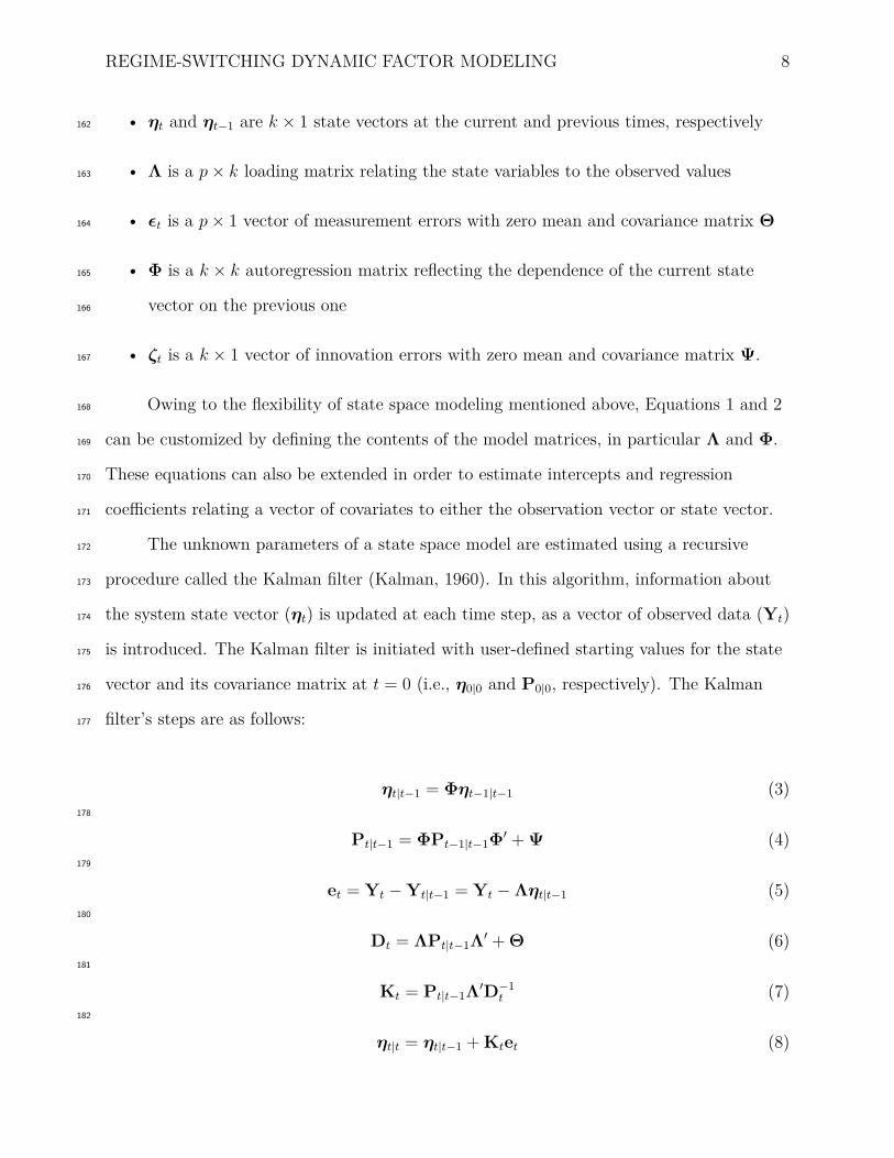
Estimation of the state vector and regime at each time step, as well as the model251

parameters, is performed using the Kim filter (Kim & Nelson, 1999) and maximum252

likelihood estimation. The Kim filter is a combination of the Kalman filter (Kalman, 1960)253

and the Hamilton filter (Hamilton, 1989). In a regime-switching model, the Hamilton filter254

enables the probabilistic inference of the regimes, which are also unobserved, based on the255

behavior of the observed time series. The Kim filter deploys these algorithms in three256

steps. First, the Kalman filter is used to generate an estimate of the state vector and its257

REGIME-SWITCHING DYNAMIC FACTOR MODELING 13

covariance matrix. Second, the Hamilton filter is used to obtain the joint probability of258

Regime i at time t − 1 and Regime j at time t (i.e., Pr[Rt−1 = i, Rt = j|Yt]), as well as the259

probability of Regime j at time t (i.e., Pr[Rt = j|Yt]). Third, a so-called collapsing process260

combines the estimates from the first two steps. Prediction errors are obtained as261

byproducts of the Kim filter and passed to the prediction error decomposition function262

(Equation 10), which is entered into an optimization step to obtain the parameter263

estimates. For each iteration of the optimization routine, the Kim filter is carried out264

recursively for all t (1, 2, . . . , T ) so that the state vector and regime probabilities have been265

estimated at each time step. Although a full and detailed coverage of these algorithms is266

beyond the scope of this paper, details can be obtained from other sources (Kim & Nelson,267

1999; Yang & Chow, 2010). The estimated parameters of the RSDFM include the factor268

loadings for Regime 2 (λ2, . . . , λp), measurement error variances for each regime269

(θ11, . . . , θp1, θ12, . . . , θp2), one or two autoregression coefficients for the latent collective270

variable (φ1, φ2), the innovation error variance (ψ), and the natural log odds of the regime271

transition probabilities (ln( πij

1−πij)).272

Interpreting the Parameters of the RSDFM273

It may be of substantive value to researchers to quantify the magnitude and274

prevalence of behavioral similarity. Magnitude is the extent to which the individuals in a275

collective are synchronized in terms of the variable of interest. Within the RSDFM276

approach, magnitude may be interpreted from the effect sizes attributed to the individuals277

in a collective. Effect size refers to the proportion of variance in each observed time series278

explained by the collective state variable, and as such, its value may range from 0 to 1. In279

the current formulation of the RSDFM, effect size for each individual is equal to 1 minus280

the unexplained variance (i.e., measurement error variance) in Regime 2, which is also281

equal to the Regime 2 standardized factor loading squared. Regime 1 is formulated with282

zero factor loadings (i.e., no collective process driving the observed time series), and hence,283

REGIME-SWITCHING DYNAMIC FACTOR MODELING 14

should have 100% unexplained variance. That is, the confidence intervals of the Regime 1284

measurement error variances should all include 1. In sum, an effect size between 0 and 1285

will be estimated for each individual for Regime 2, and this will quantify the magnitude of286

speed similarity, or the extent to which each individual’s time series reflects the collective,287

within the high similarity regime. Individual effect sizes can be averaged to obtain an288

aggregate measure of magnitude for the collective. As an alternative approximation of289

magnitude, and/or for comparison, the researcher may assess the correlation coefficients for290

all pairs of collective members (e.g., teammates) separately for each of the predicted291

regimes.292

It may also be useful to quantify speed similarity’s prevalence, which we define as the293

proportion of time in which a collective resides in Regime 2 (i.e., the high similarity294

regime). The RSDFM approach yields a prediction of Regime 1 or Regime 2 at every time295

point, making it straightforward to assess the prevalence of high similarity. This can be296

easily computed as the number of time points at which Regime 2 was predicted, divided by297

the total number of time points. This proportion (or percentage, if reported as such) is298

often referred to as the dwell time of a system within a particular state, in this case the299

high similarity regime. In the next sections, dwell time will be reported as the main metric300

of prevalence. The estimated regime transition probabilities (πij) can also indicate whether301

Regimes 1 and 2 are well balanced or one regime is relatively dominant over an analyzed302

time interval. For example, if π11 is estimated to be .75 and π22 is estimated to be .99, this303

suggests that Regime 2 is dominant. That is, Regime 2 is so prevalent that when the304

collective resides in this high similarity state, there is only a .01 probability of switching to305

Regime 1 at the next time point. In contrast, when the collective is classified as residing in306

Regime 1, there is a .25 probability of switching to Regime 2. These approaches to307

examining and reporting the magnitude and prevalence of behavioral similarity are308

demonstrated in the empirical study reported in the next section.309

REGIME-SWITCHING DYNAMIC FACTOR MODELING 15

Application: Speed Similarity in Women’s Soccer Players310

Method311

Participants, Procedures, and Materials. Varsity women’s soccer players were312

recruited from a National Collegiate Athletic Association (NCAA) Division I team in the313

United States. The university’s Institutional Review Board approved the study protocol314

detailing the recruitment of participants and data collection procedures. The number of315

players who gave informed consent to participate in the study was 25. Data were collected316

during the team’s competitive 2017 season, including all 18 regular season home and away317

games. Only outfield players were included in the study; goalkeepers were excluded. For318

each game, participants who started the game and played without substitution until319

halftime were included. Therefore, out of the ten outfield players starting each game, some320

were excluded due to first half substitutions and the fact that some starters may not have321

been consenting participants. The actual sample size for each of the 18 games ranged from322

3 to 9 participants (median = 6). Data from the second half of games were not used due to323

practical issues such as the halftime break and the prevalence of second half substitutions.324

In this study, the collective is the unit of analysis, and data were collected in the325

team’s natural competitive setting without any researcher interference. That is, in each326

game it was solely the team’s coaching staff who determined which individuals played, so327

the study participants vary from game to game. A unique identification code was randomly328

assigned to each participant for the purpose of recording which individuals started each329

game. However, for the purposes of the analyses performed, the identities of the individuals330

participating in each game and their playing positions (e.g., defender, midfielder, forward)331

are not accounted for. In terms of how the analyses were carried out, the individual332

participants can be assumed to be interchangeable. For example, the symbol used to333

represent player 4 (i.e., y4) may, in different games, refer to different individuals. Likewise,334

data from the same individual may, for example, be denoted as y1 in one game and y3 in335

another game.336

REGIME-SWITCHING DYNAMIC FACTOR MODELING 16

Data were collected using the Polar® Team Pro system (Polar Electro, Inc., Kempele,337

Finland). This system consists of a chest strap monitor worn by each participant and a338

tablet computer application with an interface that enables real-time performance tracking.339

The wearable devices include GPS tracking, accelerometers, and heart rate monitoring, and340

the data are delivered to the online application using Bluetooth technology. The system341

was owned and used regularly by the team during training and competitive games. Team342

members each had their own numbered device, and at the outset of the study all343

participants already had training and experience wearing the monitors properly. Data344

streams including acceleration, running cadence, cumulative distance, and heart rate were345

available for download after each game. In this study the variables of interest are cadence346

and distance. Data sets were downloaded following each game, then processed and347

analyzed, as detailed next.348

Data Processing and Analysis. Cadence data streams were recorded at a rate of349

1 Hz in units of revolutions per minute (rpm), where one revolution equals two steps (e.g.,350

80 rpm = 160 steps per minute). Cumulative distance was recorded at 10 Hz in units of351

yards. The cumulative distance time series were converted to distances covered within352

defined time intervals, or bins, by differencing the cumulative values. Similarly, cadence353

time series were aggregated by taking the mean cadence within each bin. Time series were354

examined for order of ARMA process using plots of the autocorrelation function (ACF)355

and partial ACF (PACF) and by running univariate ARMA models on individual time356

series. The R (R Core Team, 2017) functions acf, pacf, and arima were used to perform357

these diagnostics. If the ACF has a significant autocorrelation persisting over many lags358

(i.e., decays gradually), and the PACF becomes non-significant abruptly after a smaller359

number of lags, then this is indicative of an AR process (Bowerman, O’Connell, & Koehler,360

2005). ACF and PACF plots for this study are included in Figure 1. Inspecting these plots361

to guide our assessment of ARMA order, we treated the significance thresholds (dashed362

lines) as approximate but not strict cutoffs. Most of the individual time series, both for363

REGIME-SWITCHING DYNAMIC FACTOR MODELING 17

cadence and distance, exhibited ACFs and PACFs reflecting an AR(1) process (Panels D &364

F of Figure 1) or an AR(2) process (Panels B, H, L). Much less common were AR(3)365

processes (Panel J), so only AR(1) and AR(2) models were used in this study.366

(FIGURE 1 NEAR HERE)367

Determining an appropriate sampling rate (i.e., bin size) for the data requires368

balancing a tradeoff between scientific and practical considerations. In terms of scientific369

considerations, it is desirable to sample data frequently enough to reflect the time scale of370

interest to examine changes in the observed variables (Collins & Graham, 2002; Smith &371

Walls, 2016; Walls, Barta, Stawski, Collyer, & Hofer, 2012). In terms of practical372

considerations, data sampled very close together may have features such as repetition of373

the same or very similar values (i.e., high autocorrelation) and may therefore exhibit374

nonstationarity. Ultimately, both cadence and distance time series were aggregated in bins375

of 3 seconds due to issues with nonstationarity that became apparent when using bins of 1376

or 2 seconds. This was evident in part by the large number of models that failed to377

converge. Of the models that did successfully converge, the estimated AR coefficients were378

very close to, and their confidence intervals covered, the boundaries of stationarity379

conditions. That is, for AR(1) models, the parameter φ1 estimates were close to 1, and for380

AR(2) models, the sums of the parameter φ1 and φ2 estimates were close to 1. These381

problems were no longer apparent after reducing the sampling rate by increasing the bin382

size to 3 seconds. Given that observations were taken from the first half (45 minutes) of383

each soccer game, using a bin size of 3 seconds yielded time series each with 900384

observations. Finally, before analysis each time series was intraindividually standardized,385

that is, converted to z-scores. Doing so enables straightforward interpretation of each386

measurement error variance estimate as the proportion of variance in the observations not387

explained by the latent collective variable and is consistent with previous regime-switching388

applications (e.g., Chow, Witkiewitz, Grasman, Hutton, & Maisto, 2014; Chow,389

Witkiewitz, Grasman, & Maisto, 2015). Moreover, speed similarity should not be affected390

REGIME-SWITCHING DYNAMIC FACTOR MODELING 18

by intraindividual standardization because similarity is modeled as covariation, not as391

sameness of players’ actual levels of cadence or distance. However, it is unknown what392

effect standardization might have on the standard error estimates, so this is an important393

area of future research (see Conclusion).394

In this study, in addition to a two-regime RSDFM characterizing the presence of zero395

and high similarity regimes, it is also considered that a one-regime model, that is, a396

non-switching (high similarity only) dynamic factor model (DFM), may provide better fit397

than the RSDFM. For all analyses, we used the dynr R package (Ou, Hunter, & Chow,398

2018); code included in supplementary online resource. The variables cadence and distance399

were analyzed separately for each of the 18 games (i.e., 36 unique data sets). With a400

typical laptop, analyzing each variable (fitting 4 models for each of 18 games) took401

approximately 1.5 hours. For each data set, the best fitting model was selected by402

comparing Akaike Information Criterion (AIC; Akaike, 1998) and Bayesian Information403

Criterion (BIC; Schwarz, 1978) fit indices. When comparing AIC or BIC values for models404

fit to a given data set, smaller values indicate better model fit. In sum, one best fitting405

model (AR(1) DFM, AR(2) DFM, AR(1) RSDFM, or AR(2) RSDFM) was selected for406

each game/variable combination based on the lowest AIC/BIC value (see Tables 1 and 2).407

There were some models that converged but had non-positive definite Hessian matrices,408

which meant that the standard errors were computed using a nearest positive definite409

approximation to the Hessian matrix, and hence were not trustworthy. These models were410

discarded and not considered for selection.411

Results412

In general, AIC and BIC were in agreement of the best fitting model for each data413

set, so only AIC values are displayed in Tables 1 and 2. One exception was the analysis of414

cadence data from Game 17, where the AR(2) RSDFM produced the smallest AIC, while415

the AR(2) one-regime model produced the smallest BIC. In that case, the RSDFM was416

REGIME-SWITCHING DYNAMIC FACTOR MODELING 19

Game N AR(1)DFM

AR(2)DFM

AR(1)RSDFM

AR(2)RSDFM

Selected Model

1 8 17105 16969 - - AR(2)DFM2 6 12702 12586 12634 12530 AR(2)RSDFM3 9 - 19116 19168 - AR(2)DFM4 5 10956 - - - AR(1)DFM5 5 10286 10204 10211 10125 AR(2)RSDFM6 6 11808 11674 11761 - AR(2)DFM7 7 15258 15162 - 15098 AR(2)RSDFM8 9 19396 19262 - - AR(2)DFM9 7 - 15144 - - AR(2)DFM10 6 12995 12872 12956 14580 AR(2)DFM11 8 - - - 17591 AR(2)RSDFM12 7 14240 14116 14104 13984 AR(2)RSDFM13 4 7798 7727 7791 7667 AR(2)RSDFM14 6 12934 12816 12891 - AR(2)DFM15 7 - 15179 - - AR(2)DFM16 5 11400 11284 11342 11238 AR(2)RSDFM17 4 8566 8483 8556 8468 AR(2)RSDFM18 3 - 6666 6674 6596 AR(2)RSDFM

Note: The selected model for each data set (table row) is that with the smallest AIC value;missing AIC indicates that the model failed to converge during estimation or was discarded

Table 1Cadence models: sample sizes (N), AIC, selected model.

selected. AR(2) models were more commonly selected than AR(1) models for both417

variables analyzed. One striking difference between the analyses for cadence and distance is418

the number of regime-switching models (RSDFMs) selected over one-regime models419

(DFMs). Out of the 18 selected models used to analyze cadence, there were 9 RSDFMs420

and 9 DFMs. Out of the 17 selected models for distance (for Game 15, no model was421

selected), 14 were RSDFMs and 3 were DFMs.422

Next, we present detailed results of one exemplar analysis each for cadence and423

distance. These include the Game 7 cadence data and Game 12 distance data. In both of424

the examples, the AR(2) RSDFM was the selected model. Parameter estimates from the425

AR(2) RSDFM fit to the Game 7 cadence data can be found in Table 3. Some individual426

differences are apparent in the magnitudes (effect sizes) associated with individual players.427

REGIME-SWITCHING DYNAMIC FACTOR MODELING 20

Game N AR(1)DFM

AR(2)DFM

AR(1)RSDFM

AR(2)RSDFM

Selected Model

1 8 17026 16934 16651 16565 AR(2)RSDFM2 6 12656 12590 12517 12440 AR(2)RSDFM3 9 18934 18837 18745 - AR(1)RSDFM4 5 - 10822 10753 - AR(1)RSDFM5 5 10115 10066 10004 9958 AR(2)RSDFM6 6 11935 11874 11778 11687 AR(2)RSDFM7 7 14935 14877 - 14755 AR(2)RSDFM8 9 18809 18687 18699 - AR(2)DFM9 7 - 14918 14892 14804 AR(2)RSDFM10 6 13159 13044 12948 12828 AR(2)RSDFM11 8 17263 17141 17147 - AR(2)DFM12 7 14319 14193 14087 13965 AR(2)RSDFM13 4 7742 7695 7621 7567 AR(2)RSDFM14 6 - 13302 13228 - AR(1)RSDFM15 7 - - - - None16 5 11399 11265 11307 - AR(2)DFM17 4 - 8634 8235 8200 AR(2)RSDFM18 3 6703 6628 6598 6532 AR(2)RSDFM

Note: The selected model for each data set (table row) is that with the smallest AIC value;missing AIC indicates that the model failed to converge during estimation or was discarded

Table 2Distance models: sample sizes (N), AIC, selected model.

That is, the collective state variable explains a higher proportion of variance in some428

individuals’ cadence compared to others. This is reflected by the standardized loadings,429

which can be squared to obtain effect sizes. For example, the standardized loading430

associated with y2 is .20 (i.e., effect size of .04, unexplained variance of .96 in Regime 2),431

which may point to this individual lacking in similarity, in terms of cadence, with the rest432

of her teammates. This is also evident in Table 4, which displays the empirical bivariate433

correlations in cadence time series during predicted Regime 1 (“Zero”; Panel a) and434

predicted Regime 2 (“High”; Panel b) intervals. In Panel b, it is clear that correlations435

involving y2 tend to be smaller than others. As expected, the correlations displayed in436

Table 4 tend to be higher in predicted Regime 2 intervals, compared to their Regime 1437

counterparts in Panel a, which tended to be smaller and, in some cases, negative. The438

REGIME-SWITCHING DYNAMIC FACTOR MODELING 21

Parameter Symbol Est. SE t 95% CI pL1 fixed (std.) λ1 1.00 (.81) - - - -L2 unstd. (std.) λ2 .30 (.20) .05 6.6 (.21 , .39) <.001L3 unstd. (std.) λ3 .75 (.62) .04 16.7 (.66 , .83) <.001L4 unstd. (std.) λ4 .90 (.70) .04 21.1 (.82 , .98) <.001L5 unstd. (std.) λ5 1.10 (.90) .04 29.4 (1.03 , 1.18) <.001L6 unstd. (std.) λ6 .60 (.54) .04 13.9 (.52 , .68) <.001L7 unstd. (std.) λ7 .92 (.77) .04 22.5 (.84 , 1.00) <.001MEV1 reg. 1 θ11 .87 .14 6.4 (.61 , 1.14) <.001MEV2 reg. 1 θ21 .86 .15 5.8 (.57 , 1.15) <.001MEV3 reg. 1 θ31 1.09 .18 6.1 (.74 , 1.44) <.001MEV4 reg. 1 θ41 .65 .11 5.8 (.43 , .87) <.001MEV5 reg. 1 θ51 .91 .14 6.7 (.64 , 1.17) <.001MEV6 reg. 1 θ61 1.28 .22 5.7 (.84 , 1.72) <.001MEV7 reg. 1 θ71 1.24 .19 6.6 (.87 , 1.61) <.001MEV1 reg. 2 θ12 .34 .02 14.0 (.29 , .39) <.001MEV2 reg. 2 θ22 .96 .05 18.9 (.86 , 1.06) <.001MEV3 reg. 2 θ32 .61 .04 15.8 (.54 , .69) <.001MEV4 reg. 2 θ42 .51 .03 16.4 (.45 , .57) <.001MEV5 reg. 2 θ52 .19 .02 11.5 (.16 , .23) <.001MEV6 reg. 2 θ62 .71 .04 16.2 (.62 , .80) <.001MEV7 reg. 2 θ72 .40 .03 14.5 (.35 , .46) <.001AR1 coefficient φ1 1.30 .05 27.8 (1.21 , 1.39) <.001AR2 coefficient φ2 -.49 .04 -12.5 (-.57 , -.41) <.001IE var. ψ .12 .01 8.4 (.09 , .15) <.001Log odds 1→1 ln( π11

1−π11) 1.23 .28 4.5 (.69 , 1.78) <.001

Log odds 2→1 ln( π211−π21

) -3.38 .28 -11.9 (-3.94 , -2.82) <.001

Note: CI = confidence interval; Est. = estimate; IE = innovation error; L = loading; MEV =measurement error variance; p = p-value; reg. = regime; SE = standard error; std. =standardized; t = Student’s t test statistic; unstd. = unstandardized; var. = variance

Table 3Parameter estimates from AR(2) RSDFM fit to Game 7 cadence data.

REGIME-SWITCHING DYNAMIC FACTOR MODELING 22

y1 y2 y3 y4 y5 y6

y2 .19y3 -.20 .10y4 -.06 -.11 .35y5 .45 .08 -.38 -.10y6 .16 .19 -.06 -.11 .00y7 -.27 -.25 .34 .22 -.13 -.39(a) “Zero” similarity intervals (predicted Regime 1)

y1 y2 y3 y4 y5 y6

y2 .19y3 .39 .18y4 .51 .20 .51y5 .74 .17 .48 .63y6 .42 .11 .34 .36 .43y7 .56 .16 .54 .49 .67 .33(b) “High” similarity intervals (predicted Regime 2)

Table 4Empirical correlations in cadence in Game 7, by predicted regime.

empirical correlations in Panel a demonstrate that a zero similarity regime may not fit the439

data well in terms of covariation in pairs of teammates (e.g., a correlation between y1 and440

y5 of .45 and between y6 and y7 of -.39).441

The log odds of the regime transition probabilities suggest that Regime 2 was442

dominant, according to the AR(2) RSDFM. The estimated value of -3.38 for ln( π211−π21

)443

equates to a probability of switching from Regime 2 to Regime 1 of only .034, and444

therefore, the probability of staying in the high similarity Regime 2 is estimated to be .966.445

On the other hand, the estimated value of 1.23 for ln( π111−π11

) in Table 3 would convert to446

π11 = .774, which is not a very high probability of staying in the zero similarity Regime 1.447

The prevalence of Regime 2 is quite apparent in the top panel of Figure 2, which shows the448

Game 7 cadence time series superimposed on the predicted regimes. In this analysis, the449

team was predicted to reside in the high similarity regime with a dwell time of .91 (i.e., 820450

out of the 900 time points). In the bottom panel of Figure 2, the plot is zoomed in on 30451

REGIME-SWITCHING DYNAMIC FACTOR MODELING 23

time points to show time series data in each predicted regime. The individual time series452

appear to vary independently of one another when Regime 1 is predicted (white region)453

and show more similar patterns of variation when Regime 2 is predicted (shaded region).454

(FIGURE 2 NEAR HERE)455

Results of the analysis of Game 12 distance data, using an AR(2) RSDFM, can be456

found in Table 5. Unlike in the previous example, the standardized loadings are all457

relatively high, ranging from .57 to .87 (.32 to .75 when squared to evaluate effect size, or458

magnitude). This suggests a large proportion of variance in players’ distance explained by459

the collective state variable, that is, a large magnitude of speed similarity. The smallest of460

the standardized loadings (.57, or 32% explained variance) is consistent with the slightly461

lower correlation coefficients including y5 in Table 6(b), although this individual difference462

is not as striking as in the previous example. In other words, there is some indication that463

y5 may not be synchronized to her teammates as well as they are to each other, in terms of464

distance covered in Game 12. As expected, the correlation coefficients in Table 6(a) are low465

and/or negative, but their counterparts in Panel b are higher and entirely positive.466

As in the previous example, “staying probabilities” predicted by the AR(2) RSDFM467

for the Game 12 distance data (π11 = .579; π22 = .946), and the predicted regimes468

themselves (see Figure 3, top panel), show that the high similarity Regime 2 is far more469

prevalent than Regime 1. In this example, the team was predicted to reside in Regime 2 for470

857 out of 900 time points (i.e., dwell time = .95). In the bottom panel of Figure 3, the471

plot is zoomed in on 30 time points to juxtapose the behavior of time series in predicted472

Regime 1 against Regime 2. Again, the time series appear to behave more similarly in the473

shaded region and less so in the area with a white background.474

(FIGURE 3 NEAR HERE)475

Having inspected the results of two models in detail, next we present aggregate476

information about the magnitude and prevalence of speed similarity reflected by the477

selected model results, across the entire season. In particular, to summarize the magnitude478

REGIME-SWITCHING DYNAMIC FACTOR MODELING 24

Parameter Symbol Est. SE t 95% CI pL1 fixed (std.) λ1 1.00 (.71) - - - -L2 unstd. (std.) λ2 .94 (.81) .05 19.7 (.84, 1.03) <.001L3 unstd. (std.) λ3 1.15 (.84) .05 22.6 (1.05, 1.25) <.001L4 unstd. (std.) λ4 .94 (.81) .05 2.2 (.85, 1.04) <.001L5 unstd. (std.) λ5 .81 (.57) .05 16.0 (.71, .91) <.001L6 unstd. (std.) λ6 1.03 (.86) .05 21.9 (.93, 1.12) <.001L7 unstd. (std.) λ7 .99 (.87) .05 21.8 (.90, 1.08) <.001MEV1 reg. 1 θ11 .69 .14 5.0 (.42, .96) <.001MEV2 reg. 1 θ21 1.97 .31 6.3 (1.36, 2.59) <.001MEV3 reg. 1 θ31 .67 .13 5.3 (.43, .92) <.001MEV4 reg. 1 θ41 1.85 .30 6.2 (1.26, 2.43) <.001MEV5 reg. 1 θ51 .61 .13 4.8 (.36, .85) <.001MEV6 reg. 1 θ61 2.14 .35 6.0 (1.44, 2.83) <.001MEV7 reg. 1 θ71 2.26 .36 6.3 (1.56, 2.96) <.001MEV1 reg. 2 θ12 .49 .03 17.3 (.43, .54) <.001MEV2 reg. 2 θ22 .35 .02 16.0 (.31, .40) <.001MEV3 reg. 2 θ32 .30 .02 15.2 (.26, .34) <.001MEV4 reg. 2 θ42 .35 .03 13.1 (.29, .40) <.001MEV5 reg. 2 θ52 .68 .04 18.1 (.60, .75) <.001MEV6 reg. 2 θ62 .26 .02 15.1 (.23, .30) <.001MEV7 reg. 2 θ72 .25 .02 14.8 (.21, .28) <.001AR1 coefficient φ1 1.26 .04 29.4 (1.18, 1.34) <.001AR2 coefficient φ2 -.50 .04 -12.4 (-.58, -.42) <.001IE var. ψ .12 .01 8.8 (.10, .15) <.001Log odds 1→1 ln( π11

1−π11) .32 .24 1.3 (-.15, .79) .091

Log odds 2→1 ln( π211−π21

) -2.91 .19 -15.3 (-3.28, -2.53) <.001

Note: CI = confidence interval; Est. = estimate; IE = innovation error; L = loading; MEV =measurement error variance; p = p-value; reg. = regime; SE = standard error; std. =standardized; t = Student’s t test statistic; unstd. = unstandardized; var. = variance

Table 5Parameter estimates from AR(2) RSDFM fit to Game 12 distance data.

REGIME-SWITCHING DYNAMIC FACTOR MODELING 25

y1 y2 y3 y4 y5 y6

y2 .01y3 .03 .14y4 .22 .15 .10y5 .16 -.37 -.24 .19y6 .10 -.11 -.02 -.23 .00y7 .18 .27 .15 .26 -.04 .07(a) “Zero” similarity intervals (predicted Regime 1)

y1 y2 y3 y4 y5 y6

y2 .48y3 .61 .64y4 .52 .55 .63y5 .48 .35 .48 .47y6 .56 .62 .71 .57 .39y7 .52 .66 .65 .73 .42 .62(b) “High” similarity intervals (predicted Regime 2)

Table 6Empirical correlations in distance in Game 12, by predicted regime.

of similarity, we focus on mean effect sizes (i.e., proportion of variance explained by the479

collective state variable) and bivariate correlations between teammate pairs (i.e., in zero vs.480

high predicted regimes). To summarize the prevalence of similarity, we present dwell time481

proportions in the high similarity regime. In Figure 4, overlapping histograms depict the482

distribution of bivariate correlations between teammate pairs for selected regime-switching483

models. The histograms represent bivariate correlations from all 9 of the selected RSDFMs484

analyzing cadence data and all 14 of the selected RSDFMs analyzing distance data. As485

expected, the distributions of correlation coefficients for Regime 1 are approximately486

centered on zero, and the distributions for Regime 2 are approximately centered on .5, with487

only positive values.488

(FIGURE 4 NEAR HERE)489

Figures 5 and 6 is display prevalence and magnitude, respectively, over the course of490

the 18-game season. Although it is not possible to examine temporal trends due to the491

REGIME-SWITCHING DYNAMIC FACTOR MODELING 26

many variables (individuals involved, opponent, location, conditions, etc.) that may differ492

for each game, it is clear that Regime 2 was overwhelmingly prevalent in all of the analyses493

(i.e., greater than .88 dwell time for all 23 of the selected RSDFMs). A possible494

explanation for the dominance of Regime 2 is addressed in the Discussion section. The495

magnitudes in Figure 6 are displayed as the mean effect sizes, that is, the means of the496

squared standardized loadings for all selected models, both DFMs and RSDFMs. The497

mean effect sizes mostly range from .4 to .6 throughout the season.498

(FIGURES 5 AND 6 NEAR HERE)499

Discussion500

The analysis of cadence and distance data sets from college women’s soccer produced501

several important outcomes worthy of discussion, both at the level of specific analyses and502

at the aggregate level. To exemplify the substantively relevant details that can be503

extracted from each analysis, we presented two sets of results using the RSDFM approach504

(Game 7 cadence and Game 12 distance). One characteristic of a team’s speed similarity505

that is likely to have scientific and practical value is the magnitude of similarity. In506

particular, standardized loadings, when squared, equal the effect size, the proportion of507

variance in each observed time series explained by the collective state variable. This can be508

interpreted as the extent of each individual’s similarity with the collective. In the Game 7509

example, it was noted that one individual’s cadence (y2) was not as well synchronized to510

the collective as the cadences of the other six members. The small standardized loading511

(.20) and small bivariate correlations between y2 and each other time series in predicted512

Regime 2 supported this finding. Hence, with this analytical approach it is possible to513

identify individuals who contribute more or less than others to behavioral similarity, which514

has practical value to those affiliated with teams such as coaches, performance analysts,515

sport psychologists, and the athletes themselves. Additionally, presenting specific examples516

made it possible to show didactically how the bivariate correlations among time series can517

REGIME-SWITCHING DYNAMIC FACTOR MODELING 27

be inspected separately for the two predicted regimes for comparison, and how the518

estimated regime switching probabilities (πij) and proportion of dwell time reflect the519

prevalence of each regime. Plotting the predicted regimes is also useful to visualize the520

prevalence of each regime.521

Other important outcomes of the study can be examined at the aggregate level. This522

is useful, as in the case of this study, when analyzing behavioral similarity within many523

measurement epochs (e.g., games) spanning a longer time period (e.g., a sports season).524

First, to aggregate information about the magnitude of speed similarity over all games in525

which a regime-switching model was selected, we generated overlapping histograms to526

compare the distribution of bivariate correlations in the predicted Regime 1 versus Regime527

2. This confirmed what one might expect, that is, smaller correlations centered on zero in528

Regime 1, and larger positive correlations centered on .5 in Regime 2. Second, the mean529

effect sizes, computed by averaging the squared standardized loadings from each selected530

model, can be plotted for the 18-game season. In this application, there was substantial531

heterogeneity in games (in terms of players, opponents, conditions, etc.) that would have532

hindered our ability to assess longitudinal trends in speed similarity, but under more533

controlled conditions, researchers may choose to investigate questions such as: Does the534

average magnitude of a group’s behavioral similarity change over time? Third, we535

emphasized the proportion of time spent in each regime (i.e., dwell time) as a substantively536

valuable outcome to assess the prevalence of high similarity when using RSDFMs. At the537

aggregate level, dwell time proportions can be plotted, for example, for all games in a538

season to check for changes over time.539

We reported a large percentage of time spent in the high similarity regime (i.e.,540

greater than 88%). This finding is likely due to the constraints of competitive soccer. That541

is, particularly at the highest levels of competitive sport, the movements of teammates are542

often constrained to be highly similar. The observed variables cadence and distance were543

used in this study to operationalize speed of movement. In competitive soccer, in which544

REGIME-SWITCHING DYNAMIC FACTOR MODELING 28

team members are typically arranged in and trained to maintain a particular formation, it545

would be expected, and beneficial to performance, for teammates to move in similar546

directions and at similar speeds in response to events in the game such as the position of547

the ball and the team in possession. Indeed, it is difficult to envision a team achieving548

success with some players standing still, others walking, others jogging, and others549

sprinting. Put another way, it would be detrimental to the team’s overall performance if550

individuals’ speeds were uncorrelated, that is, if they did not reside in the high similarity551

regime for a large proportion of time points. Given the context of NCAA Division I552

competition, it is appropriate that the proportions of dwell time in the high similarity553

regime were so high. In other contexts or at other levels of expertise, it may be of554

substantive interest to rigorously test whether a collective can show improvements over555

time, in terms of dwell time in a high similarity state.556

Conclusion557

This paper featured didactic presentation of a regime-switching dynamic factor558

analytic approach and an empirical application. This inquiry produced several important559

developments in the study of collective synchrony. First, unlike most other synchrony560

applications, which tend to focus on dyads, here we have employed a multivariate approach561

to enable the examination of behavioral similarity in groups of three or more. Our data562

included teams of various sizes ranging from three to nine. Second, as opposed to studies563

that have used metrics to quantify synchrony over the duration of a time interval as a564

single aggregate value, we used a regime-switching approach to account for temporal565

changes between states of high and zero similarity. Third, the dynamic factor modeling566

approach used in this study enabled the weighting of each individual player’s unique567

influence on the team’s behavioral similarity. These weights, or factor loadings, can be568

squared to obtain effect sizes (i.e., proportions of explained variance), which quantify the569

magnitude of similarity. These can be examined on an individual basis and summarized for570

REGIME-SWITCHING DYNAMIC FACTOR MODELING 29

all team members by computing the mean of their values, for example. Fourth, by571

categorizing time intervals as residing within either a high or zero similarity regime, this572

modeling approach allows the researcher to extract information about the prevalence of573

behavioral similarity. That is, what proportion of time (i.e., dwell time) is spent in the574

high similarity regime over a given time interval analyzed? We have shown how these575

features, magnitude and prevalence, can be aggregated and depicted graphically in order to576

summarize multiple epochs of observation over a longer time period.577

In terms of the methodological aim, this investigation has demonstrated the value of578

the RSDFM approach to analyzing behavioral similarity. In our application, it was579

apparent that the parameter estimates and predicted regimes can be useful to directly580

interpret about a single time interval (e.g., dwell time within one game; magnitude of581

similarity of one player’s behavior with that of the collective), and to aggregate for a larger582

set of events (e.g., many games within a season). Substantively, two findings are583

particularly noteworthy. First, each player’s unique contribution to behavioral similarity584

can be detected in the form of a standardized factor loading. The practical significance of585

this cannot be overstated. This implies that stakeholders interested in team performance586

(e.g., coaches, analysts, players, support staff) could use this information to identify and587

address possible weaknesses in terms of behavioral similarity. Second, the large dwell time588

proportions of the high similarity regime observed in college women’s soccer players’589

running cadences and distances is notable. In earlier text, we suggested that this is likely590

due to the task constraints of high-level competitive soccer.591

The above methodological and substantive findings are salient in the fledgling science592

of collective synchrony, and they point to multiple avenues for future work. Regarding the593

methodological approach, first, simulation studies are needed to systematically evaluate the594

RSDFM approach under varying conditions such as number of persons, number of time595

points, frequency of regime switching, and other model parameters. Simulations in which596

skewness, kurtosis, and model error are manipulated would shed light on the robustness of597

REGIME-SWITCHING DYNAMIC FACTOR MODELING 30

estimation and model selection when the assumption of normality is violated. It will also598

be important to investigate whether intraindividual standardization affects the standard599

error estimates. This issue is well documented in structural equation modeling (Cudeck,600

1989; Krane & McDonald, 1978), but it is unclear whether it applies in state space601

modeling. Second, more application is needed with multivariate time series exhibiting602

greater balance in behavioral similarity, unlike in our empirical application where the high603

similarity regime dominated. Third, it would be worthwhile to assess the value of604

approaching the regime-switching framework as a continuous time model (Voelkle & Oud,605

2013). This may be particularly advantageous when observations are not equally spaced606

and/or when individuals within a collective are observed over the same time period but not607

at the exact same time points. Fourth, multifactor models may be useful to assess whether608

there are “sub-collectives” within a team. In other words, are there subgroups within a609

team that demonstrate similarity such as attackers/defenders or left/central/right610

positions? Fifth, beyond magnitude and prevalence, which we highlighted as two important611

features, it may be worthwhile to explore the stability of behavioral similarity. That is, for612

what duration does a team typically reside in one regime before switching to the other?613

Sixth, selecting an overall ARMA order for multi-subject time series models is a broad and614

difficult challenge (see also Rovine & Walls, 2006) that needs to be addressed. Finally,615

from a methods perspective, it is important to consider whether a RSDFM can be616

formulated to effectively detect more subtle regime changes (e.g., medium vs. low vs.617

none). It may be advantageous to establish guidelines for determining absolute cutoffs to618

differentiate between low similarity and no similarity. In this paper, we have used effect619

size (explained variance) and correlation to quantify the magnitude of similarity.620

Leveraging null hypothesis significance testing (i.e., p-values and confidence intervals) is a621

possibility for establishing a cutoff between low and no similarity. For example, one622

possibility is to create pseudo-collectives by randomly drawing time series from different623

games, then computing confidence intervals of correlations among these unrelated time624

REGIME-SWITCHING DYNAMIC FACTOR MODELING 31

series, in order to characterize a state of no similarity.625

There are numerous possible substantive directions for future research. More studies626

are needed to understand the relationship between team performance and collective627

physiological synchrony, for example. This has been the focus of a few studies (Elkins et628

al., 2009; Henning, Boucsein, & Gil, 2001; Strang, Funke, Russell, Dukes, & Middendorf,629

2014), but this relationship is still not well understood. As it was suggested in the630

introduction of this paper, an important future direction will be to control for copresence,631

characteristics of the shared task, and/or coordination, in order to tease out the effect of632

each on collective behavioral and physiological synchrony. Understanding the unique role633

of each antecedent in the context of team performance would have tremendous scientific634

and practical importance. For example, to what extent is collective synchrony in635

physiology related to interindividual matching of emotion, and not simply a byproduct of636

the metabolic demands of physical exertion? It would also be useful to investigate637

collective synchrony in other variables not included in this paper such as players’ direction638

of movement (i.e., change in longitudinal and lateral position). Another critical question639

that remains is whether behavioral similarity can be developed within a team (i.e., can a640

team gain expertise in it, and can it be trained?). Finally, another important remaining641

issue for future research is to clarify what specifically is the relationship between behavioral642

similarity and collective flow. If collective flow is an outcome of behavioral similarity as we643

have rendered previously (Smith, 2018), then it is plausible that regime changes in644

behavioral similarity may reflect the emergence/departure of collective flow states.645

Although there is still much to uncover about how and why behavioral similarity manifests646

during team performance, this paper has taken some very important steps to establish a647

framework for scholarly inquiry in the field.648

REGIME-SWITCHING DYNAMIC FACTOR MODELING 32

References649

Akaike, H. (1998). Information theory and an extension of the maximum likelihood650

principle. In Selected papers of hirotugu akaike (pp. 199–213). Springer.651

Araújo, D., Davids, K., & Hristovski, R. (2006). The ecological dynamics of decision652

making in sport. Psychology of Sport and Exercise, 7 (6), 653–676.653

Bowerman, B., O’Connell, R. T., & Koehler, A. B. (2005). Forecasting, time series, and654

regression: An applied approach (4th ed.). Cincinnati, OH: South-Western College655

Pub.656

Cannon-Bowers, J., Tannenbaum, S., Salas, E., & Volpe, C. (1995). Defining competencies657

and establishing team training requirements. In R. Guzzo & E. Salas (Eds.), Team658

effectiveness and decision making in organizations (pp. 333–380). San Francisco, CA:659

Jossey-Bass.660

Chow, S.-M., Ho, M.-H. R., Hamaker, E. L., & Dolan, C. V. (2010). Equivalence and661

differences between structural equation modeling and state-space modeling662

techniques. Structural Equation Modeling, 17 , 303–332.663

Chow, S.-M., Witkiewitz, K., Grasman, R., Hutton, R. S., & Maisto, S. A. (2014). A664

regime-switching longitudinal model of alcohol lapse-relapse. In P. C. M. Molenaar,665

R. M. Lerner, & K. M. Newell (Eds.), Handbook of developmental systems theory and666

methodology (pp. 397–424). Guilford Press.667

Chow, S.-M., Witkiewitz, K., Grasman, R., & Maisto, S. A. (2015). The cusp catastrophe668

model as cross-sectional and longitudinal mixture structural equation models.669

Psychological Methods, 20 (1), 142–164.670

Collins, L. M., & Graham, J. W. (2002). The effect of the timing and spacing of671

observations in longitudinal studies of tobacco and other drug use: Temporal design672

considerations. Drug & Alcohol Dependence, 68 , 85–96.673

Cudeck, R. (1989). Analysis of correlation matrices using covariance structure models.674

Psychological Bulletin, 105 (2), 317–327.675

REGIME-SWITCHING DYNAMIC FACTOR MODELING 33

Duarte, R., Araújo, D., Correia, V., & Davids, K. (2012). Sports teams as superorganisms:676

implications of sociobiological models of behaviour for research and practice in team677

sports performance analysis. Sports Medicine, 42 (8), 633–642. doi:678

10.2165/11632450-000000000-00000679

Duarte, R., Araújo, D., Correia, V., Davids, K., Marques, P., & Richardson, M. J. (2013).680

Competing together: Assessing the dynamics of team-team and player-team681

synchrony in professional association football. Human Movement Science, 32 (4),682

555–566. doi: 10.1016/j.humov.2013.01.011683

Durbin, J., & Koopman, S. J. (2012). Time series analysis by state space methods (Second684

ed.).685

Elkins, A. N., Muth, E. R., Hoover, A. W., Walker, A. D., Carpenter, T. L., & Switzer,686

F. S. (2009). Physiological compliance and team performance. Applied Ergonomics,687

40 (6), 997–1003. doi: 10.1016/j.apergo.2009.02.002688

Engle, R., & Watson, M. (1981). A one-factor multivariate time series model of689

metropolitan wage rates. Journal of the American Statistical Association, 76 (376),690

774–781. doi: 10.1080/01621459.1981.10477720691

Feldman, R. (2003). Infant–mother and infant–father synchrony: The coregulation of692

positive arousal. Infant Mental Health Journal, 24 (1), 1–23.693

Hamaker, E. L., & Grasman, R. P. P. P. (2012). Regime switching state-space models694

applied to psychological processes: Handling missing data and making inferences.695

Psychometrika, 77 (2), 400–422.696

Hamilton, J. D. (1989). A new approach to the economic analysis of nonstationary time697

series and the business cycle. Econometrica: Journal of the Econometric Society,698

357–384.699

Harvey, A. C. (1989). Forecasting, structural time series models and the kalman filter.700

Cambridge, UK: Cambridge University Press.701

Hatfield, E., Cacioppo, J. T., & Rapson, R. L. (1993). Emotional contagion. Current702

REGIME-SWITCHING DYNAMIC FACTOR MODELING 34

Directions in Psychological Science, 2 (3), 96–100.703

Henning, R. A., Boucsein, W., & Gil, M. C. (2001). Social-physiological compliance as a704

determinant of team performance. International Journal of Psychophysiology, 40 (3),705

221–232. doi: 10.1016/S0167-8760(00)00190-2706

Ho, M.-H. R., Shumway, R., & Ombao, H. (2006). The state space approach to modeling707

dynamic processes. In T. A. Walls & J. L. Schafer (Eds.), Models for intensive708

longitudinal data (pp. 148–175). New York, NY: Oxford. doi:709

10.1093/acprof:oso/9780195173444.001.0001710

Hunter, M. D. (2018). State space modeling in an open source, modular, structural711

equation modeling environment. Structural Equation Modeling: A Multidisciplinary712

Journal, 25 (2), 307–324.713

Jones, R. H. (1993). Longitudinal data with serial correlation: a state-space approach.714

London, UK: Chapman & Hall Press.715

Kalman, R. E. (1960). A new approach to linear filtering and prediction problems. Journal716

of Basic Engineering, 82 (1), 35–45.717

Kim, C. J., & Nelson, C. R. (1999). State-space models with regime switching: classical and718

gibbs-sampling approaches with applications. Cambridge, MA: MIT Press.719

Krane, W. R., & McDonald, R. P. (1978). Scale invariance and the factor analysis of720

correlation matrices. British Journal of Mathematical and Statistical Psychology,721

31 (2), 218–228.722

López-Felip, M. A., Davis, T. J., Frank, T. D., & Dixon, J. A. (2018). A cluster phase723

analysis for collective behavior in team sports. Human Movement Science, 59 ,724

96–111. doi: 10.1016/j.humov.2018.03.013725

Molenaar, P. C. M. (1985). A dynamic factor model for the analysis of multivariate time726

series. Psychometrika, 50 (2), 181–202. doi: 10.1007/BF02294246727

Nesselroade, J. J., McArdle, J. J., Aggen, S. H., & Meyers, J. H. (2002). Dynamic factor728

analysis models for representing process in multivariate time-series. In729

REGIME-SWITCHING DYNAMIC FACTOR MODELING 35

D. M. Moskowitz & S. L. Hershberger (Eds.), Modeling intraindividual variability730

with repeated measures data: Methods and applications (pp. 233–266). Mahwah, NJ:731

Erlbaum.732

Ou, L., Hunter, M. D., & Chow, S.-M. (2018). dynr: Dynamic modeling in r [Computer733

software manual]. Retrieved from https://CRAN.R-project.org/package=dynr (R734

package version 0.1.12-5)735

Palumbo, R. V., Marraccini, M. E., Weyandt, L. L., Wilder-Smith, O., McGee, H. A., Liu,736

S., & Goodwin, M. S. (2017). Interpersonal autonomic physiology: A systematic737

review of the literature. Personality and Social Psychology Review, 21 (2), 99–141.738

doi: 10.1177/1088868316628405739

R Core Team. (2017). R: A language and environment for statistical computing [Computer740

software manual]. Vienna, Austria. Retrieved from http://www.R-project.org/741

Rovine, M. J., & Walls, T. A. (2006). Multilevel autoregressive modeling of interindividual742

differences in the stability of a process. In T. A. Walls & J. L. Schafer (Eds.), Models743

for intensive longitudinal data (pp. 127–147). New York, NY: Oxford.744

Schwarz, G. (1978). Estimating the dimension of a model. The Annals of Statistics, 6 (2),745

461–464.746

Shumway, R. H., & Stoffer, D. S. (2010). Time series analysis and its applications: with r747

examples. Springer Science & Business Media.748

Smith, D. M. (2018). Collective synchrony in team sports (Unpublished doctoral749

dissertation). University of Rhode Island.750

Smith, D. M., & Walls, T. A. (2016). Multiple time scale models in sport and exercise751

science. Measurement in Physical Education and Exercise Science, 20 (4), 185–199.752

Strang, A. J., Funke, G. J., Russell, S. M., Dukes, A. W., & Middendorf, M. S. (2014).753

Physio-behavioral coupling in a cooperative team task: Contributors and relations.754

Journal of Experimental Psychology: Human Perception and Performance, 40 (1),755

145–159.756

REGIME-SWITCHING DYNAMIC FACTOR MODELING 36

Voelkle, M. C., & Oud, J. H. (2013). Continuous time modelling with individually varying757

time intervals for oscillating and non-oscillating processes. British Journal of758

Mathematical and Statistical Psychology, 66 (1), 103–126.759

Walls, T. A., Barta, W. D., Stawski, R. S., Collyer, C., & Hofer, S. M. (2012).760

Time-scale-dependent longitudinal designs. In B. Laursen, T. D. Little, & N. A. Card761

(Eds.), Handbook of developmental research methods (pp. 46–64). New York, NY:762

Guilford.763

Walls, T. A., & Schafer, J. L. (Eds.). (2006). Models for intensive longitudinal data. New764

York, NY: Oxford.765

Wiltermuth, S. S., & Heath, C. (2009). Synchrony and cooperation. Psychological Science,766

20 (1), 1–5.767

Yang, M., & Chow, S.-M. (2010). Using state-space model with regime switching to768

represent the dynamics of facial electromyography (EMG) data. Psychometrika,769

75 (4), 744–771.770

REGIME-SWITCHING DYNAMIC FACTOR MODELING 37

Figure 1 . Plots of ACF and PACF of cadence (upper 3 rows) and distance (lower 3 rows)time series data; each row shows ACF (left) and PACF (right) side-by-side for a randomlyselected participant; dashed lines indicate p = .05 significance limits.

REGIME-SWITCHING DYNAMIC FACTOR MODELING 38

Figure 2 . Game 7 cadence data superimposed on predicted regimes; full time series (toppanel) and zoomed in (bottom panel).

REGIME-SWITCHING DYNAMIC FACTOR MODELING 39

Figure 3 . Game 12 distance data superimposed on predicted regimes; full time series (toppanel) and zoomed in (bottom panel).

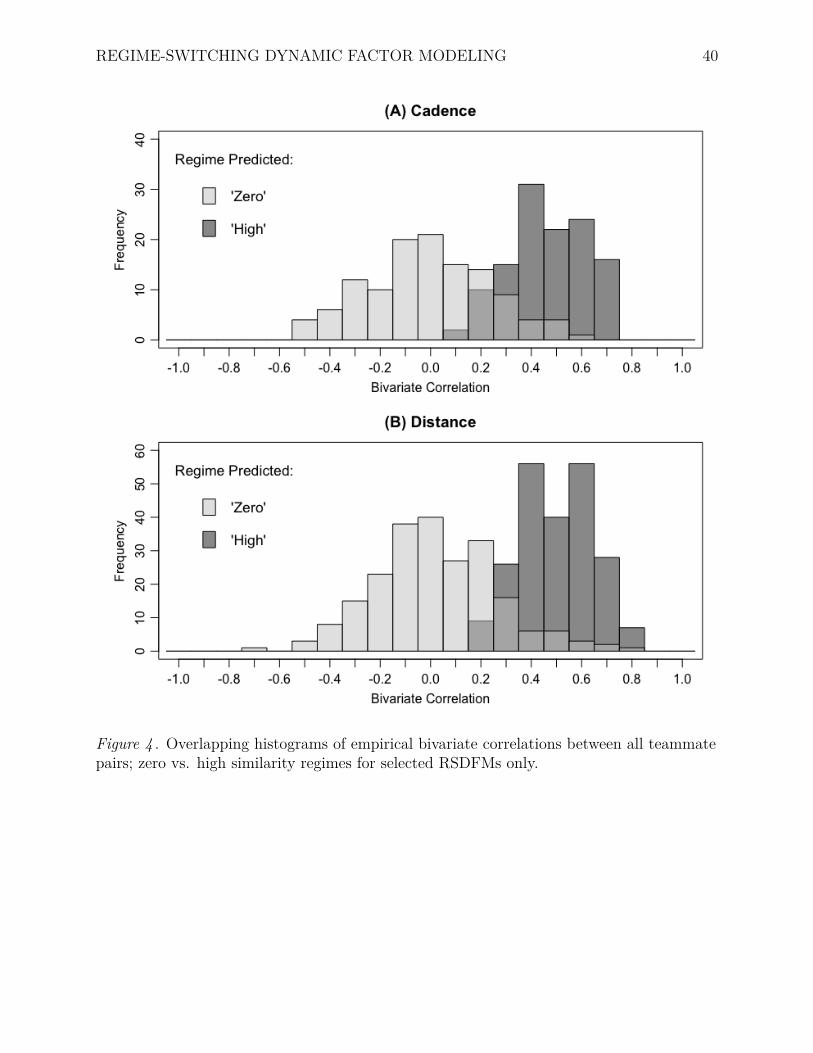
REGIME-SWITCHING DYNAMIC FACTOR MODELING 40

Figure 4 . Overlapping histograms of empirical bivariate correlations between all teammatepairs; zero vs. high similarity regimes for selected RSDFMs only.

REGIME-SWITCHING DYNAMIC FACTOR MODELING 41

Figure 5 . Proportion dwell time in high similarity regime, over 18 games.

REGIME-SWITCHING DYNAMIC FACTOR MODELING 42

Figure 6 . Mean effect sizes, over 18 games.


Recommended