39
PVE for MRI Brain PVE for MRI Brain Tissue Classification Tissue Classification Zeng Dong SLST, UESTC 6-9
| Date post: | 02-Jan-2016 |
| Category: |
Documents |
| Upload: | stella-mccoy |
| View: | 226 times |
| Download: | 0 times |

PVE for MRI Brain Tissue PVE for MRI Brain Tissue ClassificationClassification
Zeng DongSLST, UESTC
6-9

PVEPVEPartial Volume Effect

ContentsContents
OverviewMethod
Nei. PVE Model
MAPResultDiscussionConclusion

Overview 1-roleOverview 1-role
Roles of Segmentation
in qualitative
in visualization

Overview 2 – difficultyOverview 2 – difficulty
difficulty inhomogeneous
PVE
hard
soft segmentation • Statistic• MAP• MRF

Overview 3 - PVE Overview 3 - PVE
IEE95 NOISE MODELS based Sampling noise Material-dependent NoisePVE
direct
indirect

DirectDirect
Determine PVC directlyIEEE91
nwyK
jjii j
1
multichannel
),()( niii wgwyp
]1,0[,11
jj i
K
ji ww

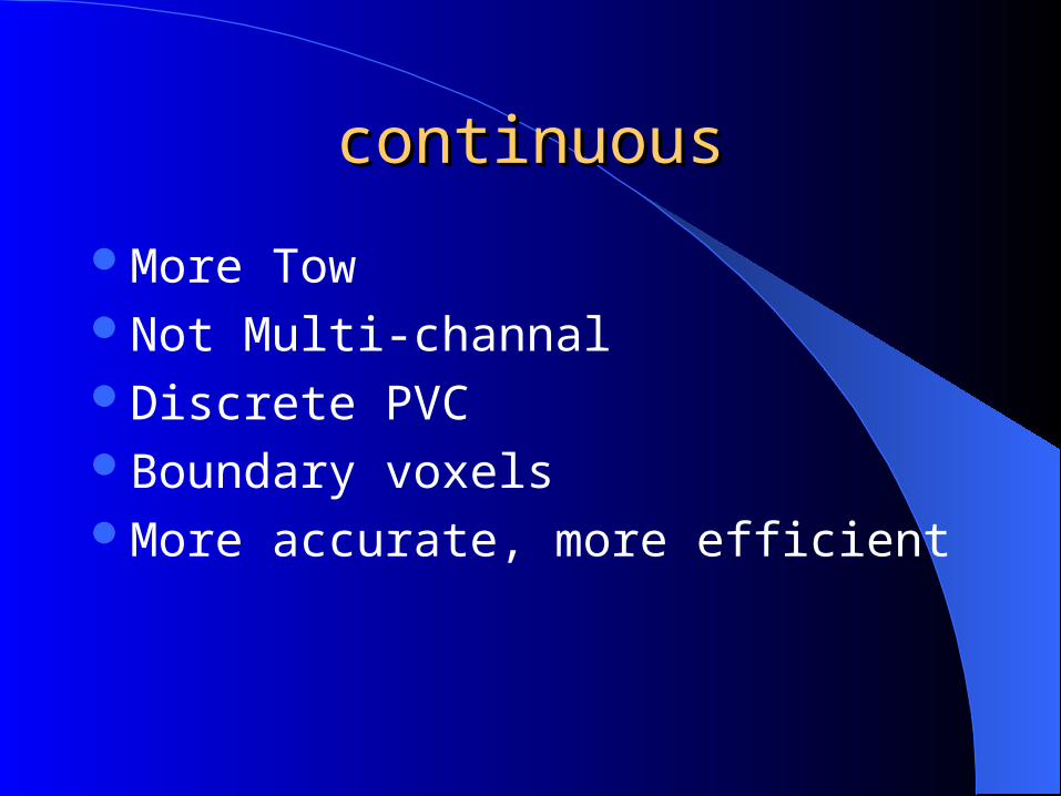
continuouscontinuous
IEE03
Only tow types

continuouscontinuous
02 Fuzzy Markov
discrete PVC

IndirectIndirect
PV classDetermine PVC based on PV voxels
),()( niii wgwyp
iw
inii dwwgyp ),()(
continuouscontinuous
More TowNot Multi-channalDiscrete PVCBoundary voxelsMore accurate, more efficient

Method-Nei. PVEMethod-Nei. PVE
},,1{ :SetIndex NS
},{ :image Obseved SiyY i
N: numbers of pixels
Assume:
},0;{H : SiyiSetIndexmask i
mask

continuouscontinuous
},,1{ :SetIndex Pure KP K: numbers of pure
j :RV Pure b ),( pj
pjg
Pjpj
pj
p ,,
g(.,.): Gaussian function

continuecontinue
Observed is mixed with its nei.s meanly during sampling
Nei. Size M
M
jii jy
My
1
1

continuecontinue
K
jjji bn
My
1
1
MnK
jj
1
],0[ Mn j

continuecontinue
L kinds of mixed types:Mixed set
Assume
LF ,,1
FlvV l , Pjnv jl , A mixed type
typel)mixed(labe therepresent RV Assume ii yx
SiFxxX ii ,; :Set Label

continuecontinue
),(),( iip
ii gxyp
K
jjji n
M 1
1
K
jjji n
M 1
1

PVE SegmentationPVE SegmentationMAP
)(arg max* YXPXX
Y: observed images
X: segmentation images
prior
likelihood
)()()( XPXYPYXP

Likelihood termLikelihood term
Assume that the intensity at voxel i does not depend on the tissue content of the other voxels.
N
i
pii xypXYP
1
),()(

PriorPrior
Assume X is MRF on nei. System C, and x is a realization RF X
))(exp(1
)( xUZ
xp
Z: Partition function
U(x): Potential energy function
Xx
xUZ ))(exp(
Cc
c xvxU )()(

continuecontinue
SNxxVxU iSi Ni
ii
i
,),()( 2
otherwiseCv
maskivvrxxV
i
ii
x
xxiiii
,
,),(
0
2
2
constant enough large a is C
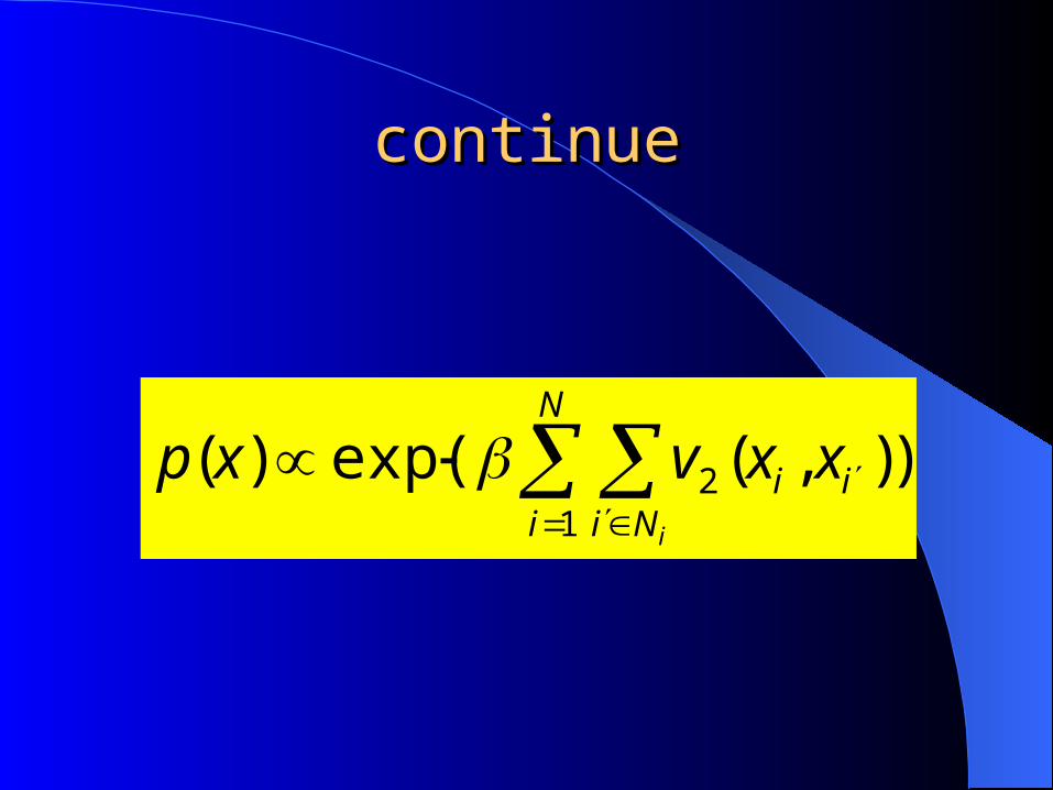
continuecontinue
)),(exp()(1
2
N
i Niii
i
xxvxp

continuecontinue
)()()( XPXYPYXP
N
i i
ii
i
N
i Niii
y
xxvi
)2
)(exp(
2
1
)),(exp(
2
12

ICMICM
Iterative Constrained Mode
local
combination

continuecontinue
iNiii
K
j
pjj
K
j
pjjiK
j
pjji
xxv
nM
nM
y
nM
U
),(
1
1
2
12
1ln
2
1
2
1
1

continuecontinue
jN
kkk
jj yyjP
N 1
)(1
2
1
22 )(1
j
N
kii
jj
j
yyjPN

continuecontinue
1. Init X (beta = 0, M=1)2. Update mixel mean and variance3. ICM4. goto 2

ResultResult
Brain tissue classification
K=3: CSF, GM, WM
N=1,3,7,27

continuecontinue
Generate Mixed types:
for CSF=M:0
for GM=(M-CSF):0 {
WM=M-CSF-GM
…
}

continuecontinue
Example(K=3,M=7)
Reduce: Not tow maximization( 3) CSF !=0 && GM != 0 (18)
1 2 3 4 5 6 7 8 9 10 11 12 13 14 15 16 17 18 19 20 21 22 23 24 25 26 27 28 29 30 31 32 33 34 35 36
CSF 7 6 6 5 5 5 4 4 4 4 3 3 3 3 3 2 2 2 2 2 2 1 1 1 1 1 1 1 0 0 0 0 0 0 0 0GM 0 1 0 2 1 0 3 1 2 0 4 3 2 1 0 5 4 3 2 1 0 6 5 4 3 2 1 0 7 6 5 4 3 2 1 0WM0 0 1 0 1 2 0 1 2 3 0 1 2 3 4 0 1 2 3 4 5 0 1 2 3 4 5 6 0 1 2 3 4 5 6 7

continuecontinue
Ori seg
Ori
Seg with b
Seg without b

continuecontinue
compare
数据 100_23 1_24 11_3 110_3 111_2 112_2 12_3 13_3 15_3* 17_3*CSF 0.3018 0.1089 0.1159 0.3101 0.3418 0.3072 0.1182 0.3097GM 0.8880 0.8460 0.8781 0.8221 0.8195 0.8056 0.9035 0.9022WM 0.8339 0.8170 0.8356 0.7757 0.7956 0.7649 0.8583 0.8529数据 17_3 191_3 202_3 205_3CSF 0.1031 0.1296 0.0891GM 0.642 0.8541 0.8924 0.8781WM 0.782 0.8263 0.8403 0.8433
Mean: csf 20% GM 86% WM :83%
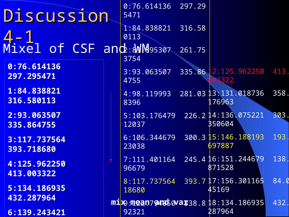
Discussion 4-1Discussion 4-1Mixel of CSF and WM
0:76.614136 297.295471
1:84.838821 316.580113
2:93.063507 335.864755
3:117.737564 393.718680
4:125.962250 413.003322
5:134.186935 432.287964
6:139.243421 377.461605
7:144.299907 322.635246
8:159.469365 158.156170
9:164.525851 103.329811
10:169.582336 48.503452
mix mean and var
0:76.614136 297.295471
1:84.838821 316.580113
2:89.895307 261.753754
3:93.063507 335.864755
4:98.119993 281.038396
5:103.176479 226.212037
6:106.344679 300.323038
7:111.401164 245.496679
8:117.737564 393.718680
9:122.794050 338.892321
10:137.963508 174.413245
11:143.019993 119.586886
12:125.962250 413.003322
13:131.018736 358.176963
14:136.075221 303.350604
15:146.188193 193.697887
16:151.244679 138.871528
17:156.301165 84.045169
18:134.186935 432.287964
19:139.243421 377.461605
20:144.299907 322.635246
21:159.469365 158.156170
22:164.525851 103.329811
23:169.582336 48.503452

continouscontinous
Mixel of CSF and WM
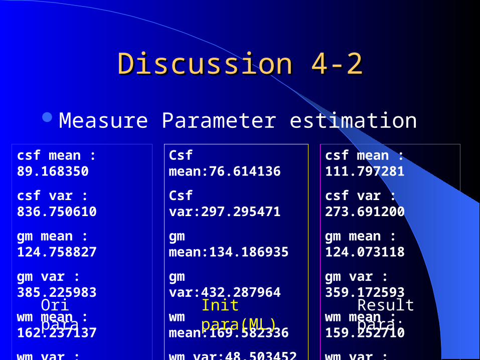
Discussion 4-2Discussion 4-2
Measure Parameter estimation
csf mean : 89.168350
csf var : 836.750610
gm mean : 124.758827
gm var : 385.225983
wm mean : 162.237137
wm var : 186.776108
csf mean : 111.797281
csf var : 273.691200
gm mean : 124.073118
gm var : 359.172593
wm mean : 159.252710
wm var : 212.954779
Result para:Ori para
Csf mean:76.614136
Csf var:297.295471
gm mean:134.186935
gm var:432.287964
wm mean:169.582336
wm var:48.503452
Init para(ML)

Discussion 4-3Discussion 4-3
Prior Parameter estimation
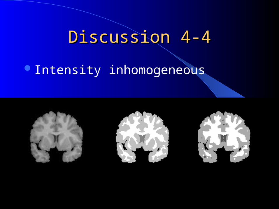
Discussion 4-4Discussion 4-4
Intensity inhomogeneous

ConclusionConclusion
More accurate, more efficientUnify frameworkgeneralization

Thanks


