PYGIST Python Interface to Gist Graphicshifweb.lbl.gov/public/software/gist/pygist.pdf · PYGIST...

UCRL-MA-128569Revision No. 5April 18, 2003

PYGIST

Python Interface to Gist Graphics

AbstractThis document describes usage of the PYGIST and GIST3D Python modules. PYGIST enables

users to access Yorick graphics functions from the Python scripting language. This moduleprovides 2D plotting capability. The separate GIST3D modules provides a set of Python functions

for interpreted 3D graphics.

Contents

1 Introduction 1

1.1 History . . . . . . . . . . . . . . . . . . . . . . . . . . . . . . . . . . . . . . . . 1

1.2 The 1.5 Update . . . . . . . . . . . . . . . . . . . . . . . . . . . . . . . . . . . . 1

1.3 Platforms . . . . . . . . . . . . . . . . . . . . . . . . . . . . . . . . . . . . . . . 2

1.4 Current Maintenance . . . . . . . . . . . . . . . . . . . . . . . . . . . . . . . . . 3

2 PyGist Installation 4

2.1 Windows . . . . . . . . . . . . . . . . . . . . . . . . . . . . . . . . . . . . . . . 4

2.2 Cygwin . . . . . . . . . . . . . . . . . . . . . . . . . . . . . . . . . . . . . . . . 5

3 User Setup and Demo 6

3.1 GISTPATH . . . . . . . . . . . . . . . . . . . . . . . . . . . . . . . . . . . . . . 6

4 Python Gist Graphics 7

4.1 PyGist 2D Graphics . . . . . . . . . . . . . . . . . . . . . . . . . . . . . . . . . . 7

4.1.1 Example 1 . . . . . . . . . . . . . . . . . . . . . . . . . . . . . . . . . . 7

4.1.2 Example 2 . . . . . . . . . . . . . . . . . . . . . . . . . . . . . . . . . . 8

4.2 PyGist 3D Graphics . . . . . . . . . . . . . . . . . . . . . . . . . . . . . . . . . . 9

4.2.1 General overview of module pl3d . . . . . . . . . . . . . . . . . . . . . . 9

4.2.2 Overview of module plwf . . . . . . . . . . . . . . . . . . . . . . . . . . 10

4.2.3 Overview of module slice3 . . . . . . . . . . . . . . . . . . . . . . . . . . 11

4.3 movie.py: PyGist 3D Animation . . . . . . . . . . . . . . . . . . . . . . . . . . . 11

ii

4.3.1 Examples . . . . . . . . . . . . . . . . . . . . . . . . . . . . . . . . . . . 12

4.4 Function Summary . . . . . . . . . . . . . . . . . . . . . . . . . . . . . . . . . . 13

5 Control Functions 20

5.1 Device Control . . . . . . . . . . . . . . . . . . . . . . . . . . . . . . . . . . . . 20

5.1.1 Window Control . . . . . . . . . . . . . . . . . . . . . . . . . . . . . . . 20

5.1.2 Changing the Window Style Interactively . . . . . . . . . . . . . . . . . . 22

5.1.3 Hard Copy and File Control . . . . . . . . . . . . . . . . . . . . . . . . . 26

5.2 Other Controls . . . . . . . . . . . . . . . . . . . . . . . . . . . . . . . . . . . . 27

5.2.1 animate: Control Animation Mode . . . . . . . . . . . . . . . . . . . . . . 27

5.2.2 palette: Set or Retrieve Palette . . . . . . . . . . . . . . . . . . . . . . . . 27

5.2.3 plsys: Set Coordinate System . . . . . . . . . . . . . . . . . . . . . . . . 28

5.2.4 redraw: Redraw X Window . . . . . . . . . . . . . . . . . . . . . . . . . 28

6 Plot Limits and Scaling 29

6.1 Setting Plot Limits . . . . . . . . . . . . . . . . . . . . . . . . . . . . . . . . . . 29

6.1.1 limits: Save or Restore Plot Limits . . . . . . . . . . . . . . . . . . . . . . 29

6.1.2 ylimits: Set y-axis Limits . . . . . . . . . . . . . . . . . . . . . . . . . . . 30

6.2 Scaling and Grid Lines . . . . . . . . . . . . . . . . . . . . . . . . . . . . . . . . 30

6.2.1 logxy: Set Linear/ Log Axis Scaling . . . . . . . . . . . . . . . . . . . . . 30

6.2.2 gridxy: Specify Grid Lines . . . . . . . . . . . . . . . . . . . . . . . . . . 31

6.3 Zooming Operations . . . . . . . . . . . . . . . . . . . . . . . . . . . . . . . . . 31

7 Two-Dimensional Plotting Functions 33

7.1 Output Primitives . . . . . . . . . . . . . . . . . . . . . . . . . . . . . . . . . . . 33

iii

7.1.1 plg: Plot a Graph . . . . . . . . . . . . . . . . . . . . . . . . . . . . . . . 33

7.1.2 plmesh: Set Default Mesh . . . . . . . . . . . . . . . . . . . . . . . . . . 34

7.1.3 plm: Plot a Mesh . . . . . . . . . . . . . . . . . . . . . . . . . . . . . . . 36

7.1.4 plc: Plot Contours . . . . . . . . . . . . . . . . . . . . . . . . . . . . . . 37

7.1.5 plv: Plot a Vector Field . . . . . . . . . . . . . . . . . . . . . . . . . . . . 38

7.1.6 plf: Plot a Filled Mesh . . . . . . . . . . . . . . . . . . . . . . . . . . . . 40

7.1.7 plfc: Plot filled contours . . . . . . . . . . . . . . . . . . . . . . . . . . . 41

7.1.8 plfp: Plot a List of Filled Polygons . . . . . . . . . . . . . . . . . . . . . . 42

7.1.9 pli: Plot a Cell Array . . . . . . . . . . . . . . . . . . . . . . . . . . . . . 43

7.1.10 pldj: Plot Disjoint Lines . . . . . . . . . . . . . . . . . . . . . . . . . . . 45

7.1.11 plt: Plot Text . . . . . . . . . . . . . . . . . . . . . . . . . . . . . . . . . 46

7.1.12 pltitle: Plot a Title . . . . . . . . . . . . . . . . . . . . . . . . . . . . . . 47

7.1.13 plh: Plot a Histogram . . . . . . . . . . . . . . . . . . . . . . . . . . . . . 48

7.2 Plot Function Keywords . . . . . . . . . . . . . . . . . . . . . . . . . . . . . . . 48

8 Inquiry and Miscellaneous Functions 53

8.1 Inquiry and Editing Functions . . . . . . . . . . . . . . . . . . . . . . . . . . . . 53

8.1.1 plq: Query Plot Element Status . . . . . . . . . . . . . . . . . . . . . . . 53

8.1.2 pledit: Change Plotting Properties . . . . . . . . . . . . . . . . . . . . . . 53

8.1.3 plremove: Remove Plot Element from Display . . . . . . . . . . . . . . . 54

8.1.4 pldefault: Set Default Values . . . . . . . . . . . . . . . . . . . . . . . . . 54

8.2 Miscellaneous Functions . . . . . . . . . . . . . . . . . . . . . . . . . . . . . . . 55

8.2.1 bytscl: Convert to Color Array . . . . . . . . . . . . . . . . . . . . . . . . 55

8.2.2 histeqscale: Histogram Equalized Scaling . . . . . . . . . . . . . . . . . 56

iv

8.2.3 meshloc: Get Mesh Location . . . . . . . . . . . . . . . . . . . . . . . . 56

8.2.4 mouse: Handle Mouse Click . . . . . . . . . . . . . . . . . . . . . . . . . 56

8.2.5 moush: Mouse in a Mesh . . . . . . . . . . . . . . . . . . . . . . . . . . . 57

8.2.6 pause: Pause . . . . . . . . . . . . . . . . . . . . . . . . . . . . . . . . . 57

9 Three-Dimensional Plotting Functions 59

9.1 Setting Up For 3D Graphics . . . . . . . . . . . . . . . . . . . . . . . . . . . . . 59

9.1.1 The Plotting List . . . . . . . . . . . . . . . . . . . . . . . . . . . . . . . 59

9.1.2 Functions For Setting Viewing Parameters . . . . . . . . . . . . . . . . . . 60

9.1.3 Lighting Parameters . . . . . . . . . . . . . . . . . . . . . . . . . . . . . 61

9.1.4 Display List . . . . . . . . . . . . . . . . . . . . . . . . . . . . . . . . . . 62

9.2 3D Graphics Control Functions . . . . . . . . . . . . . . . . . . . . . . . . . . . . 62

9.2.1 Getting a Window . . . . . . . . . . . . . . . . . . . . . . . . . . . . . . 62

9.2.2 Displaying the Gnomon . . . . . . . . . . . . . . . . . . . . . . . . . . . 62

9.2.3 Plotting the Display List . . . . . . . . . . . . . . . . . . . . . . . . . . . 63

9.2.4 The variabledraw3 and the idler . . . . . . . . . . . . . . . . . . . . . . 64

9.3 Data Setup Functions for Plotting . . . . . . . . . . . . . . . . . . . . . . . . . . . 65

9.3.1 Creating a Plane . . . . . . . . . . . . . . . . . . . . . . . . . . . . . . . 65

9.3.2 Creating a mesh3 argument . . . . . . . . . . . . . . . . . . . . . . . . . 65

9.4 The Slicing Functions . . . . . . . . . . . . . . . . . . . . . . . . . . . . . . . . . 68

9.4.1 slice3mesh: Pseudo-slice for a surface . . . . . . . . . . . . . . . . . . . . 69

9.4.2 slice3: Plane and Isosurface Slices of a 3D mesh . . . . . . . . . . . . . . 70

9.4.3 slice2 and slice2x: Slicing Surfaces with planes . . . . . . . . . . . . . . . 71

9.5 The 3D Plotting Functions . . . . . . . . . . . . . . . . . . . . . . . . . . . . . . 72

v

9.5.1 plwf: plot a wire frame . . . . . . . . . . . . . . . . . . . . . . . . . . . . 72

9.5.2 pl3surf: plot a 3-D surface . . . . . . . . . . . . . . . . . . . . . . . . . . 73

9.5.3 pl3tree: add a surface to a plotting tree . . . . . . . . . . . . . . . . . . . . 75

9.6 Contour Plotting on Surfaces: plzcont and pl4cont . . . . . . . . . . . . . . . . . . 78

9.7 Animation: movie and spin3 . . . . . . . . . . . . . . . . . . . . . . . . . . . . . 80

9.7.1 The movie module and function . . . . . . . . . . . . . . . . . . . . . . . 80

9.7.2 The spin3 function . . . . . . . . . . . . . . . . . . . . . . . . . . . . . . 82

9.8 Syntactic Sugar: Some Helpful Functions . . . . . . . . . . . . . . . . . . . . . . 83

9.8.1 Specifying the palette to be split: splitpalette . . . . . . . . . . . . . . . . 83

9.8.2 Saving and restoring the view and lighting: save3, restore3 . . . . . . . . . 83

10 Acknowledgements 86

A Useful Functions for Developers 87

A.1 Find 3D Lighting: get3light . . . . . . . . . . . . . . . . . . . . . . . . . . . . . 87

A.2 Get Normals to Polygon Set: get3normal . . . . . . . . . . . . . . . . . . . . . . 87

A.3 Get Centroids of Polygon Set: get3centroid . . . . . . . . . . . . . . . . . . . . . 88

A.4 Get Viewer’s Coordinates: get3xy . . . . . . . . . . . . . . . . . . . . . . . . . . 88

A.5 Add object to drawing list: set3object . . . . . . . . . . . . . . . . . . . . . . . . 88

A.6 Sort z Coordinates: sort3d . . . . . . . . . . . . . . . . . . . . . . . . . . . . . . 89

A.7 Set the cmax parameter: lightwf . . . . . . . . . . . . . . . . . . . . . . . . . . . 90

A.8 Return a Wire Frame Specification: xyzwf . . . . . . . . . . . . . . . . . . . . . 90

A.9 Calculate Chunks of Mesh: iterator3 . . . . . . . . . . . . . . . . . . . . . . . . . 91

A.10 Get Vertex Values of Function: getv3 . . . . . . . . . . . . . . . . . . . . . . . . . 91

vi

A.11 Get Cell Values of Function: getc3 . . . . . . . . . . . . . . . . . . . . . . . . . . 92

A.12 Controlling Points Close to the Slicing Plane:slice2precision . . . . . . . . . . . 93

A.13 Scale variables to a palette: bytscl, splitbytscl . . . . . . . . . . . . . . . . . . . . 93

A.14 Return Vertex Coordinates for a Chunk: xyz3 . . . . . . . . . . . . . . . . . . . . 94

A.15 Find Corner Indices of List of Cells: tocorners3 . . . . . . . . . . . . . . . . . . . 94

A.16 Timing: timer , timer print . . . . . . . . . . . . . . . . . . . . . . . . . . . . . . 94

B Maintenance: Things You Really Didn’t Want to Know 96

B.1 The Workhorse: gistCmodule . . . . . . . . . . . . . . . . . . . . . . . . . . . . . 96

B.1.1 Memory Maintenance: PyObjects . . . . . . . . . . . . . . . . . . . . . . 96

B.1.2 Memory Management: ArrayObjects . . . . . . . . . . . . . . . . . . . . 98

B.1.3 Memory Management: naked memory . . . . . . . . . . . . . . . . . . . . 99

B.1.4 Computing contour curves: contour . . . . . . . . . . . . . . . . . . . . . 100

B.1.5 Computing slices: slice2, slice2x,slice2part . . . . . . . . . . . . . . . . 100

B.2 Some Yorick-like Functions: yorick.py . . . . . . . . . . . . . . . . . . . . . . . . 103

B.3 Additional Array Operations: arrayfnsmodule . . . . . . . . . . . . . . . . . . . . 104

B.3.1 Counting Occurrences of a Value: histogram . . . . . . . . . . . . . . . . 104

B.3.2 Assigning to an Arbitrary Subset of an Array: arrayset . . . . . . . . . . . 105

B.3.3 Sorting an array: indexsort . . . . . . . . . . . . . . . . . . . . . . . . . 105

B.3.4 Interpolating Values: interp . . . . . . . . . . . . . . . . . . . . . . . . . 105

B.3.5 Digitizing an array: digitize . . . . . . . . . . . . . . . . . . . . . . . . . 106

B.3.6 Reversing a Two-Dimensional array: reverse . . . . . . . . . . . . . . . . 106

B.3.7 Obtaining an Equally-Spaced Array of Floats: span . . . . . . . . . . . . . 106

B.3.8 Effective Length of an Array: nz . . . . . . . . . . . . . . . . . . . . . . . 106

vii

B.3.9 Finding Edges Cut by Isosurfaces: findmask . . . . . . . . . . . . . . . . 107

B.3.10 Order Cut Edges of a cell: construct3 . . . . . . . . . . . . . . . . . . . . 107

B.3.11 Expand cell-centered values to node-centered values: tocorners . . . . . . 107

B.4 More slice3 details . . . . . . . . . . . . . . . . . . . . . . . . . . . . . . . . . . 108

B.4.1 Standard ordering for the four types of mesh cells . . . . . . . . . . . . . . 108

B.4.2 Standard numbering of cells in a regular rectangular mesh . . . . . . . . . 109

B.4.3 How slice3 works . . . . . . . . . . . . . . . . . . . . . . . . . . . . . . . 110

C Change History for this Document 116

viii

1 Introduction

1.1 History

This documentation is a revision of the original documentation[1] with a new title.

The Python Gist Scientific Graphics Package, written by Lee Busby and Zane Motteler ofLawrence Livermore National Laboratory, is a set of Python modules for production of general sci-entific graphics. The Python Gist modulegist.py and the associated Python extensiongistCmodule.cprovide a Python interface to the Gist library and is referred to as ‘PyGist.’

Gist is a scientific graphics library written in C by David H. Munro of Lawrence LivermoreNational Laboratory. It features support for three common graphics output devices: X-Windows,(color) Postscript, and ANSI/ISO Standard Compute Graphics Metafile (CGM). The library is small(written directly to Xlib), portable, efficient, and full-featured. It produces x-y plots with “good”tick marks and tick labels, 2D quadrilateral mesh plots with contours, filled contours, vector fields,or pseudocolor maps on such meshes, and a selection of 3D plots, including wire mesh plots (trans-parent or opaque), shaded and colored surface plots, isosurface and plane cross sections of meshescontaining data, and real-time animation (moving-light sources and rotations. The 3D library ispackaged separately as the ‘Gist3D’ module.

The original Python Gist module utilized the “Numerical” package due to J. Hugunin and others.PyGist is therefore fast and able to handle large datasets. The Gist module includes an X-windowsevent dispatcher which can be dynamically added to the Python interpreter. This makes fast mouse-controlled zoom, pan, and other graphic operations available to the researcher while maintainingthe usual Python command-line interface.

1.2 The 1.5 Update

PyGist was unmaintained for a period of time, during which the three dependent componentschanged significantly:

• Yorick 1.3 evolved to Yorick 1.5 with major changes to the graphics and event handling.

• Python 1.x evolved to Python 2.x.

• Numerical package has also evolved under Paul Dubois.

1

2 1. INTRODUCTION

The major issues addressed in bringing up PyGist 1.5 were the following:

• Upgrading the C extension to be compatible with Yorick version 1.5.

• Porting the code system to wider set of platforms of current interest: including Solaris,IRIX64, OSF/1, AIX, Linux, Cygwin, and Windows.

• Getting these two products (Python and Yorick) that support event handling to cooperate inthis area.

• Simplifying the distribution of PyGist by:

– Including the required portion of Yorick in the PyGist source.

– Packaging the software using Python DistUtils.

1.3 Platforms

PyGist 1.5.x runs on the following platforms:

• AIX

• Intel Linux 1

• alpha Linux

• Windows2

• Cygwin 3

• alpha OSF/1

• Solaris

• IRIX64 (one issue)

1Michiel de Hoon has tested PyGist on i386, and Lila Chase on Pentium4 SMP (i686).2Michiel de Hoon has tested PyGist on the following: DOS command prompt, Python for Windows, PyShell, PyCrust,

PythonWin.3Michiel de Hoon has tested PyGist on Cygwin with or without X11.

1.4. CURRENT MAINTENANCE 3

1.4 Current Maintenance

The following people are currently involved in the maintenance of PyGist:

• Dave Munro, LLNL: Gist, event handling interface

• Michiel de Hoon, University of Tokyo: Cygwin and Windows ports, build facility

• Dave Grote, LBNL: contributed bug fixes

• Lila Chase, LLNL: porting, testing, documentation

2 PyGist Installation

In general, the installation consists of running the following two steps:

python setup.py configpython setup.py install

This works on Linux, Unix, Mac OS X, Cygwin, and Windows (for the latter two, see below).Some Python versions older than 2.3 contain bugs in the distutils package, and may therefore needa different installation procedure:

cd src; make clean; make config; cd ..python setup.py install

instead.

Alternatively, use the script provided:

./install (for installation in a private directory)

./llnl_install (for installation in a public LLNL directory)

2.1 Windows

For use on Windows (from the DOS prompt or using a GUI such as IDLE, PythonWin, PyCrust, orPyShell), use the Windows installer. It is available athttp://bonsai.ims.u-tokyo.ac.jp/˜mdehoon .

If you want to recompile Pygist for Windows from source, you can do so using Cygwin/MinGW.To compile, run

/cygdrive/c/Python22/python setup.py config --compiler=mingw32/cygdrive/c/Python22/python setup.py build --compiler=mingw32

Here,/cygdrive/c/Python22/python refers to Windows’s Python as seen from Cyg-win. The exact path may be different on your machine. To install Pygist for Python on Windows,run

4

2.2. CYGWIN 5

/cygdrive/c/Python22/python setup.py install

If instead you want to create the Window installer, run

/cygdrive/c/Python22/python setup.py bdist_wininst

2.2 Cygwin

For Cygwin without XFree86, the usual installation procedure is used:

python setup.py configpython setup.py install

If you want to use Cygwin with the XFree86 implementation of the X Windows System, youneed to add--x11 to these commands:

python setup.py config --x11python setup.py install --x11

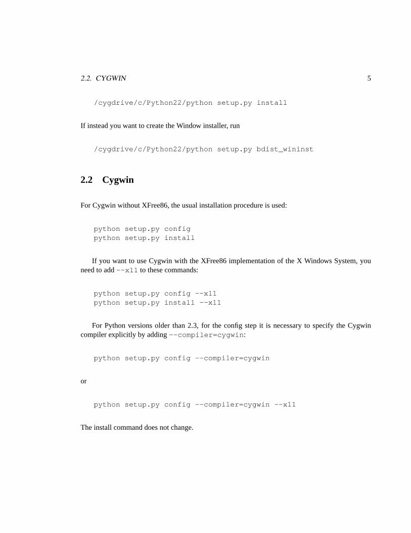
For Python versions older than 2.3, for the config step it is necessary to specify the Cygwincompiler explicitly by adding--compiler=cygwin :

python setup.py config --compiler=cygwin

or

python setup.py config --compiler=cygwin --x11

The install command does not change.

3 User Setup and Demo

At LLNL, the public version of python is installed in/usr/apps/python/opt/bin on bothopen and closed Livermore Computing computers and on the local AX-net computers. Ensure thatpython is in your path; if it is not, add:

set path = ( /usr/apps/python/opt/bin $path )

to your.cshrc if your are a CSH user, andsource the file.

There is a demonstration Python script installed in${PYTHONHOME}/lib/python2.2/site-packages/gist/gistdemolow.py , wherePYTHONHOMEis where your Python is installed; at LLNL, it is/usr/apps/python/opt .

To run the demo, type:

pythonimport gistdemolowgistdemolow.run()(ctrl-d)

3.1 GISTPATH

Gist has style files (*.gs ) and palette files (*.gp ), typically installed in a subdirectoryg wherePython is installed, and the user usually does not need to do anything else to access these files.

However, Zope users and others may require an extra setup step. For example, because Zope’sPython is installed in a non-standard location, PyGist has problems finding these files. To solve thisproblem, set the environment variable GISTPATH to the correct location of these files.

6

4 Python Gist Graphics

Gist is a scientific graphics library written in C by David H. Munro of Lawrence Livermore NationalLaboratory. It features support for three common graphics output devices: X Windows, (color)Postscript, and ANSI/ ISO Standard Computer Graphics Metafiles (CGM). The library is small(written directly to Xlib), portable, efficient, and full-featured. It produces x vs. y plots with “good”tick marks and tick labels, 2D quadrilateral mesh plots with contours, filled contours, vector fields,or pseudocolor maps on such meshes. Some 3D plot capabilities are also available. The Python Gistmodule gist. py and the Python extension gistCmodule provide a low-level Python interface to thislibrary as far as 2D is concerned. In addition, there are several other Python modules which interfacewith the 2D graphics to produce 3D graphics and animation: movie.py (supporting animation),pl3d.py (basic 3D plotting algorithms), plwf.py (wire frame plotting), and slice3.py (providing meshcapability with isosurface and plane slicing). Collectively all of these interface modules are knownas PyGist.

This chapter will summarize the plotting features that are available in PyGist, and list (in thefinal section) the functions that are to be described in future chapters.

4.1 PyGist 2D Graphics

In two dimensions, PyGist supplies functions to plot curves, meshes (with various combinations ofcontours, filled mesh cells, and vector fields on the mesh, with color-filled contours in the future),sets of filled polygons, cell arrays, sets of disjoint lines, text strings, and a title. These are allprovided by the Python module gist.py.

We will show a couple of simple examples below to give the reader a flavor of the interface.

4.1.1 Example 1

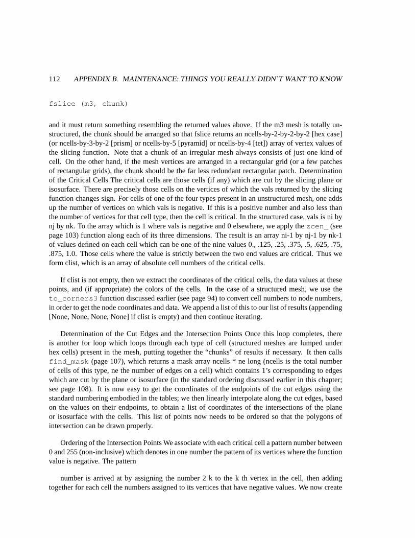
In the first example we simply plot a straight line from (1, 0) to (2, 1). Note that only two coordinatesare specified for y; x is not specified. In such a case, the values of x default to the integers from 1 tolen (y).

from gist import * # Put plot functions in name space.pldefault (marks = 1, width = 0, type = 1, style = "work.gs",

7

8 4. PYTHON GIST GRAPHICS

dpi = 100) # Set some defaults.winkill (0) # Kill any existing window.window (0, wait = 1, dpi = 75)plg ([0, 1]) # The first positional argument is y.

A

A

A

A

1.0 1.2 1.4 1.6 1.8 2.00.0

0.2

0.4

0.6

0.8

1.0

System 0

The first positional argument in PLG isy .

As can be deduced from this example, most PyGist function calls can be augmented with anumber of optional keyword arguments. These can (usually) be supplied in any order, and each isof the form keyword= value. Throughout this manual, a list of the available keywords for a functionis given with the description of the function.

4.1.2 Example 2

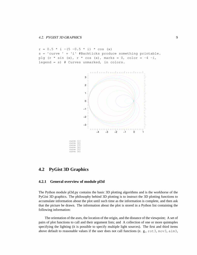
The next example computes and plots a set of nested cardioids in the primary and secondary colors.

fma()x = 2 * pi * arange (200, typecode = Float) / 199.0for i in range (1, 7):

4.2. PYGIST 3D GRAPHICS 9

r = 0.5 * i -(5 -0.5 * i) * cos (x)s = ’curve ’ + ‘i‘ #Backticks produce something printable.plg (r * sin (x), r * cos (x), marks = 0, color = -4 -i,legend = s) # Curves unmarked, in colors.

−4 −3 −2 −1 0 1

−3

−2

−1

0

1

2

3

curve [1]curve [2]curve [3]curve [4]curve [5]curve [6]

4.2 PyGist 3D Graphics

4.2.1 General overview of module pl3d

The Python module pl3d.py contains the basic 3D plotting algorithms and is the workhorse of thePyGist 3D graphics. The philosophy behind 3D plotting is to instruct the 3D plotting functions toaccumulate information about the plot until such time as the information is complete, and then askthat the picture be drawn. The information about the plot is stored in a Python list containing thefollowing information:

The orientation of the axes, the location of the origin, and the distance of the viewpoint; A set ofpairs of plot functions to call and their argument lists; and A collection of one or more quintuplesspecifying the lighting (it is possible to specify multiple light sources). The first and third itemsabove default to reasonable values if the user does not call functions (e. g.,rot3 , mov3, aim3 ,


set3_ light ., etc.) to set them. The list described in the second bullet is built by a set of oneor more calls to the various plotting functions, which create the list of arguments for each call andthen add the function name and argument list pair to the plot list for future execution. When the listis complete, a call to draw3 causes the list to be traversed, and at this point each plotting functionon the list executes with the argument list that was built when it was first called.

4.2.2 Overview of module plwf

The main function of interest in plwf.py is the function plwf (“plot wire frame”), which enables theuser to plot an arbitrary wire frame on a quadrilateral grid. The grid may be see-through or not (cellsfilled with the background color). In the latter case, the drawing order of the zones is determined bya simple “painter’s algorithm”, which works fairly well if the mesh is reasonably nearly rectilinear,but can fail even then if the viewpoint is chosen to produce extreme fisheye perspective effects. Onemust look at the resulting plot carefully to be sure the algorithm has correctly rendered the model ineach case.

A 3D wire mesh can also be plotted using shading and lighting effects as determined by valuesset in the pl3d module; or the zones can be colored (using the current palette) by their average heightor by the values of some function, which may be zone-centered or node-centered.

Examples

The following is a fairly simple example of a wire mesh plot.

from pl3d import *set_draw3_(0)x = span (-1, 1, 64, 64)y = transpose (x)z = (x + y) * exp (-6.*(x* x+ y* y))orient3 ()light3 ()from plwf import *plwf (z, y, x)[xmin, xmax, ymin, ymax] = draw3(1)limits (xmin, xmax, ymin, ymax)

Calling set_draw3_ with argument zero tells the 3d plotting routines not to draw the graphuntil asked (by a call to draw3). orient3 and light3 set the orientation and lighting parameters to

4.3. MOVIE.PY: PYGIST 3D ANIMATION 11

default values when called with no arguments. (light3 is irrelevant for this durface, since it is notshaded.) The plwf call puts this surface on the drawing list (plwf = “plot wire frame.”) The draw3call then causes the drawing list to be plotted. draw3 returns the maxima and minima of the x andy variables, which must then be sent to the limits function to prevent the plot appearing distorted.(Ah, the perils of using low level graphics.)

4.2.3 Overview of module slice3

Module slice3.py contains two plotting functions of interest. First, pl3surf can be used for graphingsurfaces on an arbitrary two-dimensional mesh with filled cells and no mesh lines. (Currently plwfcan be used to do the same thing in the case of a mesh all of whose cells are quadrilateral, andhas more flexibility, in that it allows mesh lines to be drawn and/ or allows for the mesh to be see-through.) Secondly, pl3tree is a plotting function that can be called multiple times in order to haveseveral surfaces drawn on the same graph. pl3tree (as its name suggests) creates a tree of valuessorted as to when they will be plotted on the screen; if the algorithm works correctly, then moredistant cells are plotted first, then covered by closer cells which are plotted later, giving the surfacethe correct appearance.

Surfaces to be plotted by pl3surf or pl3tree can be generated by taking plane sections of anarbitrary mesh or by creating isosurfaces for some function or functions defined on the mesh. Theseplanes and isosurfaces can themselves be sliced and portions discarded, to enhance visibility of theinterior. The functions mesh3 and slice3mesh take raw input data and put it into the form acceptedby slice3, which can form plane sections or isosurfaces through the mesh. Functions slice2 (whichreturns the portion of a surface in front of the slicing plane) and slice2x (which returns the two partsof a surface sliced by a plane) complete the triumvirate of slicing functions.

The algorithms in slice3 are independent of the underlying graphics. Thus slice3 may equallywell be used with Narcisse graphics.

4.3 movie.py: PyGist 3D Animation

The module movie.py supports 3D real time animation. Function movie accepts as argument thename of a drawing function which has as its single argument a frame number; movie then callsthis drawing function within a loop, halting when the function returns zero. The idea is that thedrawing function increments from the previous frame and draws the new frame, returning zerowhen some predefined event takes place, e. g., some set number of frames has been drawn, ora certain amount of time has elapsed. The functionspin3 in modulepl3d calls movie ; thedrawing function_spin3 draws the successive frames of a rotating 3D plot. The demonstration


module demo5.py contains an example of a shaded surface with a moving light source; the drawingfunction,demo5_light , moves the light and draws the next frame.

4.3.1 Examples

The following example is explained by comments in the code. It is taken from demo5.py. (To repeat,demo5_light is a function which appears in demo5.py.)

# First we define the mesh and functions on it.# (Note: nx == ny == nz == 20)xyz = zeros ((3, nx, ny, nz), Float)xyz [0] = multiply.outer (span (-1, 1, nx),ones ((ny, nz), Float))xyz [1] = multiply.outer (ones (nx, Float),multiply.outer (span (-1, 1, ny), ones (nz, Float)))xyz [2] = multiply.outer (ones ((nx, ny), Float),span (-1, 1, nz))r = sqrt (xyz [0] ** 2 + xyz [1] ** 2 + xyz [2] ** 2)theta = arccos (xyz [2] / r)phi = arctan2 (xyz [1] , xyz [0] + logical_not (r))y32 = sin (theta) ** 2 * cos (theta) * cos (2 * phi)# mesh3 creates an object which slice3 can slice. The# isosurfaces will be with respect to constant values# of the function r * (1. + y32)].m3 = mesh3 (xyz, funcs = [r * (1. + y32)])[nv, xyzv, dum] = slice3 (m3, 1, None, None, value = .50)# (inner isosurface)[nw, xyzw, dum] = slice3 (m3, 1, None, None, value = 1.)# (outer isosurface)pxy = plane3 (array ([ 0, 0, 1], Float), zeros (3, Float))pyz = plane3 (array ([ 1, 0, 0], Float), zeros (3, Float))[np, xyzp, vp] = slice3 (m3, pyz, None, None, 1)# (pseudo-colored plane slice)[np, xyzp, vp] = slice2 (pxy, np, xyzp, vp)# (cut slice in half, discard "back" part)[nv, xyzv, d1, nvb, xyzvb, d2] = \slice2x (pxy, nv, xyzv, None) # halve inner isosurface[nv, xyzv, d1] = \slice2 (-pyz, nv, xyzv, None)# (... halve one of those halves)

4.4. FUNCTION SUMMARY 13

[nw, xyzw, d1, nwb, xyzwb, d2] = \slice2x (pxy , nw, xyzw, None)# (split outer isosurface in halves)[nw, xyzw, d1] = \slice2 (-pyz, nw, xyzw, None) # discard half of one halffma () # frame advance# split_palette causes isosurfaces to be shaded in grey# scale, plane sections to be colored by function valuessplit_palette (" earth.gp")gnomon (1) # show small set of axesclear3 () # clears drawing listset_draw3_(0) # Make sure we don’t draw till ready# Create a tree of objects and put on drawing listpl3tree (np, xyzp, vp, pyz)pl3tree (nvb, xyzvb)pl3tree (nwb, xyzwb)pl3tree (nv, xyzv)pl3tree (nw, xyzw)orient3 ()# set lighting parameters for isosurfaceslight3 (diffuse = .2, specular = 1)limits (square= 1)demo5_light (1) # Causes drawing to appear

demo5.py also contains code which rotates the above object in real-time animation. It is notpossible to illustrate that here.

4.4 Function Summary

Here is a summary of the functions which are described in the remainder of this manual.

Control functions See page 20.

window ([n] [, <keylist>]) # open or select device nkeywords: display, dpi, dump, hcp, legends, private, style, wait

winkill ([n]) # delete device n

n = current_window () # determine active device


fma () # frame advance

Plot limits and scaling See page 29.

old_limits = limits ()

old_limits = limits (xmin [, xmax[, ymin[, ymax]]][, <keylist>])

keywords: square, nice, restrict

limits (old_limits)

ylimits (ymin[, ymax])

logxy (xflag[, yflag])

gridxy (flag)

gridxy (xflag, yflag)

zoom_factor (factor)

unzoom ()

Two-dimensional plotting functions See page 33.

plg (y [, x][, <keylist>]) # plot a graphkeywords: legend, hide, type, width, color, closed,

smooth, marks, marker, mspace, mphase, rays

plmesh ([ y, x][, ireg][, triangle= tri_array])# set default mesh

plmesh () # delete default mesh

plm ([ y, x][, ireg][, <keylist>])# plot mesh

keywords: boundary, inhibit, legend, hide, type, width,color, region

plc (z[, y, x][, ireg][, <keylist>])


# plot contourskeywords: levs, triangle, legend, hide, type, width,

color, smooth, marks, marker, mspace, mphase,region

plfc (z[, y, x][, ireg][, <keylist>])# plot filled contours

keywords: contours, colors, region, triangle, scale

plv (vy, vx[, y, x][, ireg][, <keylist>])# plot vector field

keywords: scale, hollow, aspect, legend, hide, type,width, color, smooth, marks, marker, mspace,mphase, triangle, region

plf (z[, y, x][, ireg][, <keylist>])# Plot a filled mesh

keywords: edges, ecolor, ewidth, legend, hide, region,top, cmin, cmax

plfp (z, y, x, n[, <keylist>])# Plot filled polygons

keywords: legend, hide, top, cmin, cmax

pli (z[[, x0, y0], x1, y1][, <keylist>])# Plot a cell array

keywords: legend, hide, top, cmin, cmax

pldj (x0, y0, x1, y1[, <keylist>])# Plot disjoint lines

keywords: legend, hide, type, width, color

plt (text, x, y[, <keylist>])keywords: tosys, font, height, opaque, path, justify,

legend, hide, color

pltitle (title) # Plot a title

Inquiry and Miscellaneous functions See page 53.

plq () # Query plot element status


legend_list = plq ()**** RETURN VALUE NOT YET IMPLEMENTED ****

plq (n_element[, n_contour])

properties = plq (n_element[, n_contour])

pledit ([ n_element[, n_contour],] <keylist>)# Change Plotting Properties of Current ElementThe keywords can be any of the keywords that apply to the current element.

pldefault (key1= value1, key2= value2, ...)# Set default valuesThe keywords can be most of the keywords that can be passed to the plottingcommands.Also, one can specify a larger CGM file size:pldefault (cgmfilesize=20) # default is 10 MB; reset to 20 MB

bytscl (z[, top= max_byte][, cmin= lower_cutoff][, cmax= upper_cutoff])# Convert data to color array

histeq_scale (z[, top= top_value][, cmin= cmin][,cmax= cmax]) **** NOT YET IMPLEMENTED ****# Histogram Equalized Scaling

mesh_loc (y0, x0[, y, x[, ireg]])# Get zone index of (x0, y0)

result = mouse (system, style, prompt)# Handle Mouse Click

moush ([ y, x[, ireg]])# Return zone index of point clicked in mesh

pause (milliseconds) # self-explanatory

Three-dimensional plotting functions See page 59.

orient3 (phi = angle 1 , theta = angle 2)

rot3 (xa = angle x , ya = angle y , za = angle z)


mov3 (xa = val 1 , ya = val 2 , za = val 3)

aim3 (xa = val 1 , ya = val 2 , za = val 3)

light3 (ambient= a_level, diffuse= d_level,specular= s_level, spower= n, sdir= xyz)

clear3 ()

window3 ([n] [, dump = val] [, hcp = filename])

gnomon ([onoff] [, chr = <labels>])

set_default_gnomon ([onoff])

[lims = ] draw3 ([called_as_idler = <val>])

limits (lims [0], lims [1], lims [2], lims [3])

set_draw3_ (n)

n = get_draw3_ ()

clear_idler ()

set_idler (func_name)

set_default_idler ()

call_idler ()

plane3 (< normal>, <point>)

mesh3 (x, y, z)

mesh3 (x, y, z, funcs = [f1, f2, ...], [verts = <spec>])

mesh3 (xyz, funcs = [f1, f2, ...])

mesh3 (nxnynz, dxdydz, x0y0z0, funcs = [f1, f2, ...])


slice3mesh (z [, color])

slice3mesh (nxny, dxdy, x0y0, z [, color])

slice3mesh (x, y, z [, color])

slice3 (m3, fslice, nv, xyzv [, fcolor [, flg 1 ]][, value = <val>] [, node = flg 2 ])[nverts, xyzverts, values] = slice2 (plane, nv, xyzv, vals)[nverts, xyzverts, values, nvertb, xyzvertb, valueb] =

slice2x (plane, nv, xyzv, vals)

plwf (z [, y, x] [, <keylist>])keywords: fill, shade, edges, ecolor, ewidth, cull, scale, cmax

pl3surf (nverts, xyzverts [, values] [, <keylist>])keywords: cmin, cmax

pl3tree (nverts, xyzverts [, values] [, <keylist>])keywords: plane, cmin, cmax, split

Animation functions See page 80.

movie (draw_frame [, time_limit = 120.][, min_interframe = 0.0][, bracket_time = array ([ 2., 2.], Float)][, lims = None][, timing = 0])

spin3 (nframes = 30,axis = array ([-1, 1, 0], Float),tlimit = 60.,dtmin = 0.0,bracket_time = array ([ 2., 2.], Float),lims = None,timing = 0,angle = 2. * pi)

Syntactic Sugar See page 83.

split_palette ([palette_name])


view = save3 ()

restore3 (view)

5 Control Functions

This chapter contains all the information you need to control PyGist devices. Device refers to an XWindow or a hard copy file. In addition, we describe functions which control some aspects of theappearance of the graph.

5.1 Device Control

5.1.1 Window Control

Calling Sequences...

window ([n] [, <keylist>])winkill ([n])n = current_window ()fma()

Description The window function selects device n as the current graphics device. n may range from0 to 7, inclusive. Each graphics device corresponds to an X window, a hardcopy file, or both,depending on the values of the keyword arguments described below. If n is omitted, it defaultsto the current active device, if any. window returns the number of the currently active device.winkill deletes the current graphics device, or device n if n is specified.current_windowreturns the number of the current active device, or -1 if there is none. fma frame advances thecurrent graphics device. The current picture remains displayed in the associated X window(if any) until the next element is actually plotted. An fma must be given after the last plot toa hardcopy file for that plot to appear when the file is printed.

The keywords accepted by the window function are

display, dpi, dump, hcp, legends, private, style, wait

and are described in the next subsection.

Keyword Arguments The following keyword arguments can be specified with this function. dis-play A string of the formhost: server. screen which tells where the X window willappear (for example,icf.llnl.gov: 0.0 ). If not specified, uses your default display(which it gets from your DISPLAY environment variable). Usedisplay = "" (the nullstring) to create a graphics device which has no associated X window. (You should do this ifyou want to make plots in a non-interactive batch mode.)

20

5.1. DEVICE CONTROL 21

dpi The allowed values for dpi are 75 and 100. The X window will appear on your defaultdisplay at 75 dpi, unless you specify the display and/ or dpi keywords. A dpi = 100 Xwindow is larger than a dpi = 75 X window; both represent the same thing on paper.

dump The dump keyword, if present, controls whether all colors are converted to a grayscale (dump = 0, the default), or the current palette is dumped at the beginning of eachpage of hardcopy output. Set dump to 1 if you are doing color plots. The dump keywordapplies only to the specific hardcopy file defined using the hcp keyword (see below)—use the dump keyword in thehcp_file command to get the same effect in the defaulthardcopy file.

hcp The value of this keyword is a quoted string giving a file name. By default, a graph-ics window does NOT have a hardcopy file of its own—any requests for hardcopy aredirected to the default hardcopy file, so hardcopy output from any window goes to asingle file. By specifying the hcp keyword, however, a hardcopy file unique to this win-dow will be created. If the hcp filename ends in. ps , then the hardcopy file will bea PostScript file; otherwise, hardcopy files are in binary CGM format. Usehcp = ""(the null string) to revert to the default hardcopy file (closing the window specific file, ifany).

In the next section of this manual we shall consider the hardcopy and file functions.Note that the PyGist default is to write to a hardcopy file only on demand. (See functionhcp on page 26)

legends The legends keyword, if present, controls whether the curve legends are (legends = 1,the default) or are not (legends = 0) dumped to the hardcopy file. The legends keywordapplies to all pictures dumped to hardcopy from this graphics window. Legends arenever plotted to the X window.

private By default, an X window will attempt to use shared colors, which permits severalPyGist graphics windows (including windows from multiple instances of Python) touse a common palette. You can force an X window to post its own colormap (set itscolormap attribute) with the private = 1 keyword. You will most likely have to fiddlewith your window manager to understand how it handles colormap focus if you do this.Use private = 0 to return to shared colors.

style The style keyword, if present, specifies (as a quoted string) the name of a Gist stylesheetfile; the default iswork.gs . The style sheet determines the number and location ofcoordinate systems, tick and label styles, and the like. Here are brief descriptions of theavailable stylesheets:

axes.gsaxes with labeled tick marks along bottom and left of graph. boxed.gs: lines allthe way around the plot with tick marks, labeled along bottom and left.

boxed2.gssame as boxed.gs but no tick marks on the top and right sides.

l nobox.gs no box, axes, or ticks; graph extends all the way to edge of window.

nobox.gs indistinguishable froml_nobox.gs . vg.gs: large tick marks all the wayaround the graph, but no lines, with large infrequent labels on the bottom and left.

22 5. CONTROL FUNCTIONS

vgbox.gs same as vg.gs except with lines all the way around as well

work.gs small tick marks with small, frequent labels on bottom and left, no lines.

work2.gs similar to work.gs, but no ticks along top and right. wait By default, Pythonwill not wait for the X window to become visible. Code which creates a newwindow, then plots a series of frames to that window should use wait = 1 to assurethat all frames are actually plotted.

Examples The first example ensures that an old window 0 is not hanging around, and then createsa new 100 dpi window.

winkill(0)window (0, wait = 1, dpi = 100)

The second example changes the style sheet of window 2.

window (2, style = "vgbox.gs")

5.1.2 Changing the Window Style Interactively


style = get_style()set_style(style)

Description The functionget_style() returns a set of nested dictionaries that contain the styleinformation that is currently used by the active window. The dictionary has the followingstructure:style

[’landscape’] : Set orientation to portrait (0) or landscape (1)[’legend’] :

[’x’] : NDC horizontal location of the legend box[’y’] : NDC vertical location of the legend box[’dx’] : NDC horizontal offset to 2nd column[’dy’] : NDC vertical offset to 2nd column[’nchars’] : Maximum number of characters on a line[’nlines’] : Maximum number of lines[’nwrap’] : Maximum number of lines to wrap long legends[’textStyle’] :

[’height’] : Character height in NDC, default 0.0156 (12pt)[’font’] : Text font, specified by an integer:


Courier: 0Times: 4Helvetica: 8Symbol: 12New Century: 16(add 1 for bold, 2 for italic)

[’color’] : Text color[’orient’] : Text path

(’right’, ’up’, ’left’, ’down’)[’alignH’] : Horizontal alignment

(’normal’, ’left’, ’center’, ’right’)[’alignV’] : Vertical alignment

(’normal’, ’top’, ’cap’, ’half’,’base’, ’bottom’)

[’contourlegend’] :[’x’] : NDC horizontal location of the contour legend box[’y’] : NDC vertical location of the contour legend box[’dx’] : NDC horizontal offset to 2nd column in the contour legend box[’dy’] : NDC vertical offset to 2nd column in the contour legend box[’nchars’] : Maximum number of characters on a line[’nlines’] : Maximum number of lines[’nwrap’] : Maximum number of lines to wrap long legends[’textStyle’] :

[’height’] : Character height in NDC, default 0.0156 (12pt)[’font’] : Text font, specified by an integer:

Courier: 0Times: 4Helvetica: 8Symbol: 12New Century: 16(add 1 for bold, 2 for italic)

[’color’] : Text color[’orient’] : Text path

(’right’, ’up’, ’left’, ’down’)[’alignH’] : Horizontal alignment

(’normal’, ’left’, ’center’, ’right’)[’alignV’] : Vertical alignment

(’normal’, ’top’, ’cap’, ’half’,’base’, ’bottom’)

[’systems’] : returns a list of systems, each of which is a dictionary with the keys:[’legend’] : default legend[’viewport’] : viewport size,array([left, right, bottom, top])


[’ticks’] :[’frame’] : Switch the frame on (1) or off (0)[’frameStyle’] :

[’color’] : Color of the frame[’width’] : Line width of the frame[’type’] : Line style of the frame:

(’none’, ’solid’, ’dash’, ’dot’,’dashdot’, ’dashdotdot’)

[’horizontal’] :[’nDigits’] : Number of digits for the tick labels[’nMinor’] : Number of minor tick marks[’nMajor’] : Number of major tick marks[’logAdjMinor’] : Adjustment factor for nMinor for a log scale[’logAdjMajor’] : Adjustment factor for nMajor for a log scale[’flags’] : Integer, given by the sum of

1: There are ticks at the bottom edge of the viewport2: There are ticks at the upper edge of the viewport4: Ticks are centered on the axis8: Ticks are go inward from the axis

16 : Ticks are go outward from the axis32 : There are labels at the bottom edge64 : There are labels at the upper edge

128 : There is a full grid256 : There is a single grid line at the origin512 : Alternative tick generator is used

1024 : Alternative label generator is used[’xOver’] : Horizontal position of the overflow label[’yOver’] : Vertical position of the overflow label[’labelOff’] : Offset from the edge of the viewport to the labels[’tickOff’] : Offset from the edge of the viewport to the ticks[’tickLen’] : Tick lengths in NDC[’tickStyle’] :

[’color’] : Color of the ticks[’width’] : Line width of the ticks[’type’] : Line type of the ticks


[’gridLevel’] : Level of the ticks at which the grid is drawn[’gridStyle’] :

[’color’] : Color of the grid[’width’] : Line width of the grid[’type’] : Line type of the grid



[’vertical’] :[’nDigits’] : Number of digits for the tick labels[’nMinor’] : Number of minor tick marks[’nMajor’] : Number of major tick marks[’logAdjMinor’] : Adjustment factor for nMinor for a log scale[’logAdjMajor’] : Adjustment factor for nMajor for a log scale[’flags’] : Integer, given by the sum of

1: There are ticks at the left edge of the viewport2: There are ticks at the right edge of the viewport4: Ticks are centered on the axis8: Ticks are go inward from the axis

16 : Ticks are go outward from the axis32 : There are labels at the left edge64 : There are labels at the right edge

128 : There is a full grid256 : There is a single grid line at the origin512 : Alternative tick generator is used

1024 : Alternative label generator is used[’xOver’] : Horizontal position of the overflow label[’yOver’] : Vertical position of the overflow label[’labelOff’] : Offset from the edge of the viewport to the labels[’tickOff’] : Offset from the edge of the viewport to the ticks[’tickLen’] : Tick lengths in NDC[’tickStyle’] :

[’color’] : Color of the ticks[’width’] : Line width of the ticks[’type’] : Line type of the ticks


[’gridLevel’] : Level of the ticks at which the grid is drawn[’gridStyle’] :

[’color’] : Color of the grid[’width’] : Line width of the grid[’type’] : Line type of the grid


By changing the values of the appropriate keys in the dictionarystyle , and calling theroutineset_style(style) , the style of the current window can be changed interactively.This is used in theplh routine (see page 48) to switch off the tick marks and labels belowthe horizontal axis in a histogram.


5.1.3 Hard Copy and File Control


eps (name)hcp ()hcp_file ([filename] [, dump = 0/1])filename = hcp_finish ([n])hcp_out ([n] [, keep = 0/ 1])hcpon ()hcpoff ()

Descriptions ...

eps(name)Write the picture in the current graphics window to the Encapsulated PostScriptfile name +.epsi (i. e., the suffix.epsi is added to name). The eps function requiresthe ps2epsi utility which comes with the project GNU Ghostscript program. Any hard-copy file associated with the current window is first closed, but the default hardcopy fileis unaffected. As a side effect, legends are turned off and color table dumping is turnedon for the current window. The environment variablePS2EPSI_FORMATcontains theformat for the command to start the ps2epsi program.

hcp() The hcp function sends the picture displayed in the current graphics window to thehardcopy file. (The name of the default hardcopy file can be specified usinghcp_file ;each individual graphics window may have its own hardcopy file as specified by thewindow function.)

hcp file([filename [,dump=0/1])]

Sets the default hardcopy file to filename. If filename ends with.ps , the file will bea PostScript file, otherwise it will be a binary CGM file. By default, the hardcopy filename will beAa00.cgm , or Ab00.cgm if that exists, orAc00.cgm if both exist, andso on. The default hardcopy file gets hardcopy from all graphics windows which do nothave their own specific hardcopy file (see the window function). If the dump keywordis present and nonzero, then the current palette will be dumped at the beginning of eachframe of the default hardcopy file. This is what you want to do when you want colorplots. With dump = 0, the default behavior of converting all colors to a gray scale isrestored.

filename=hcpfinish([n )] Close the current hardcopy file and return the filename. If nis specified, close the hcp file associated with window n and return its name; usehcp_finish(-1) to close the default hardcopy file.

hcp out([n [,keep=0/1])] **** NOT YET IMPLEMENTED **** Finishes the current hard-copy file and sends it to the printer. If n is specified, prints the hcp file associated with

5.2. OTHER CONTROLS 27

window n; usehcp_out(-1) to print the default hardcopy file. Unless the keep key-word is supplied and nonzero, the file will be deleted after it is processed by gist andsent to lpr.

hcpon() The hcpon function causes every fma (frame advance) function call to do an implicithcp, so that every frame is sent to the hardcopy file.

hcpoff() The hcpoff command reverts to the default “demand only” mode.

5.2 Other Controls

5.2.1 animate: Control Animation Mode

Calling Sequence...

animate([0/1])

Description Without any arguments, toggle animation mode; with argument 0, turn off animationmode; with argument 1 turn on animation mode. In animation mode, the X window associatedwith a graphics window is actually an offscreen pixmap which is bit-blitted onscreen when anfma() command is issued. This is confusing unless you are actually trying to make a movie,but results in smoother animation if you are. Generally, you should turn animation on, runyour movie, then turn it off.

5.2.2 palette: Set or Retrieve Palette

Calling Sequence...

palette (filename)palette (source_window_number)palette (red, green, blue[, gray][, query = 1]

[, ntsc = 1/0])

Description Set (or retrieve with query = 1) the palette for the current graphics window. Thefilename is the name of a Gist palette file; the standard palettes areearth.gp , stern.gp ,rainbow.gp , heat.gp , gray.gp , andyarg.gp . Use the maxcolors keyword in thepldefault command to put an upper limit on the number of colors which will be read from thepalette in filename.


In the second form, the palette for the current window is copied from window numbersource_window_number .If the X colormap for the window is private, there will still be two separate X colormaps forthe two windows, but they will have the same color values.

In the third form, red, green, and blue are 1D arrays of unsigned char (Python typecode"b" ) and of the same length specifying the palette you wish to install; the values shouldvary between 0 and 255, and your palette should have no more than 240 colors. If ntsc= 0,monochrome devices (such as most laser printers) will use the average brightness to translateyour colors into gray; otherwise, the NTSC (television) averaging will be used (.30*red .59*green+.11*blue+). Alternatively, you can specify gray explicitly.

Ordinarily, the palette is not dumped to a hardcopy file (color hardcopy is still rare and ex-pensive), but you can force the palette to dump using thewindow() or hcp_file() com-mands.

5.2.3 plsys: Set Coordinate System

Calling Sequence...

plsys(n)

Description Set the current coordinate system to number n in the current graphics window. Ifn equals 0, subsequent elements will be plotted in absolute NDC coordinates outside of anycoordinate system. The default style sheetwork.gs defines only a single coordinate system,so the only other choice is n equal 1.

You can make up your own style sheet (using a text editor) which defines multiple coordinatesystems. You need to do this if you want to display four plots side by side on a single page,for example. The standard style sheetswork2.gs andboxed2.gs define two overlayedcoordinate systems with the first labeled to the right of the plot and the second labeled to theleft of the plot. When using overlayed coordinate systems, it is your responsibility to ensurethat the x-axis limits in the two systems are identical.

5.2.4 redraw: Redraw X Window

Calling Sequence...

redraw ()

6 Plot Limits and Scaling

6.1 Setting Plot Limits

6.1.1 limits: Save or Restore Plot Limits

Calling Sequence...

old_limits = limits()old_limits = limits(xmin [, xmax[, ymin[, ymax]]]

[, <keylist>])limits(old_limits)

Description In the first form, restore all four plot limits to extreme values, and save the previouslimits in the tupleold_limits .

In the second form, set the plot limits in the current coordinate system to xmin, xmax, ymin,ymax, which may each be a number to fix the corresponding limit to a specified value, orthe string"e" to make the corresponding limit take on the extreme value of the currentlydisplayed data. Arguments may be omitted from the right end only. (But see ylimits, below,to set limits on the y-axis.)

limits() always returns a tuple of 4 doubles and an integer;old_limits[0:3] arethe previous xmin, xmax, ymin, and ymax, andold_limits[4] is a set of flags indicatingextreme values and the square, nice, restrict, and log flags. This tuple can be saved and passedback tolimits() in a future call to restore the limits to a previous state.

In an X window, the limits may also be adjusted interactively with the mouse. Drag left tozoom in and pan (click left to zoom in on a point without moving it), drag middle to pan, andclick (and drag) right to zoom out (and pan). If you click just above or below the plot, theseoperations will be restricted to the x-axis; if you click just to the left or right, the operations arerestricted to the y-axis. A shift-left click, drag, and release will expand the box you draggedover to fill the plot (other popular software zooms with this paradigm). If the rubber band boxis not visible with shift-left zooming, try shift-middle or shift-right for alternate XOR masks.Such mouse-set limits are equivalent to a limits command specifying all four limits exceptthat the unzoom command (see “Zooming Operations” on page 31) can revert to the limitsbefore a series of mouse zooms and pans.

The limits you set using the limits or ylimits functions carry over to the next plot; that is, anfma operation does not reset the limits to extreme values.

29

30 6. PLOT LIMITS AND SCALING

Keyword Arguments The following keyword arguments can be specified with this function.

square = 0/1

If present, the square keyword determines whether limits marked as extreme values will beadjusted to force the x and y scales to be equal (square= 1) or not (square= 0, the default).

nice = 0/ 1

If present, the nice keyword determines whether limits will be adjusted to nice values (nice=1) or not (nice= 0, the default).

restrict = 0/ 1

There is a subtlety in the meaning of “extreme value” when one or both of the limits on theOPPOSITE axis have fixed values: does the “extreme value” of the data include points whichwill not be plotted because their other coordinate lies outside the fixed limit on the oppositeaxis (restrict= 0, the default), or not (restrict= 1)?

6.1.2 ylimits: Set y-axis Limits

Calling Sequence...

ylimits (ymin[, ymax])

Description Set the y-axis plot limits in the current coordinate system to ymin, ymax, which mayeach be a number to fix the corresponding limit to a specified value, or the string"e" to makethe corresponding limit take on the extreme value of the currently displayed data.

Arguments may be omitted only from the right. Use limits(xmin, xmax) to accomplish thesame function for the x-axis plot limits.

Note that the corresponding Yorick function for ylimits is range. Since this word is a Pythonbuilt-in function, the name has been changed to avoid the collision.

6.2 Scaling and Grid Lines

6.2.1 logxy: Set Linear/ Log Axis Scaling

Calling Sequence...

6.3. ZOOMING OPERATIONS 31

logxy(xflag[, yflag])

Description logxy sets the linear/log axis scaling flags for the current coordinate system. xflag andyflag may be 0 to select linear scaling, or 1 to select log scaling. yflag may be omitted (butnot xflag).

6.2.2 gridxy: Specify Grid Lines

Calling Sequence...

gridxy(flag)gridxy(xflag, yflag)

Description Turns on or off grid lines according to flag. In the first form, both the x and y axesare affected. In the second form, xflag and yflag may differ to have different grid options forthe two axes. In either case, a flag value of 0 means no grid lines (the default), a value of1 means grid lines at all major ticks (the level of ticks which get grid lines can be set in thestyle sheet), and a flag value of 2 means that the coordinate origin only will get a grid line. Instyles with multiple coordinate systems, only the current coordinate system is affected. Thekeywords can be used to affect the style of the grid lines.

You can also turn the ticks off entirely. (You might want to do this to plot your own customset of tick marks when the automatic tick generating machinery will never give the ticks youwant. For example a latitude axis in degrees might reasonably be labeled “0, 30, 60, 90”, butthe automatic machinery considers 3 an “ugly” number—only 1, 2, and 5 are “pretty”—andcannot make the required scale. In this case, you can turn off the automatic ticks and labels,and use plsys, pldj, and plt to generate your own.)

To fiddle with the tick flags in this general manner, set the 0x200 bit of flag (or xflag or yflag),and “or-in” the 0x1ff bits however you wish. The meaning of the various flags is described inthework.gs Gist style sheet. Additionally, you can use the 0x400 bit to turn on or off theframe drawn around the viewport. Here are some examples:

gridxy(0x233) work.gs default settinggridxy(0, 0x200) like work.gs, but no y-axis ticks or labelsgridxy(0, 0x231) like work.gs, but no y-axis ticks on rightgridxy(0x62b) boxed.gs default setting

6.3 Zooming Operations


32 6. PLOT LIMITS AND SCALING

zoom_factor(factor)unzoom()

Descriptions zoom_factor sets the zoom factor for mouse-click zoom in and zoom out opera-tions. The default factor is 1.5; factor should always be greater than 1.0.

unzoom restores limits to their values before zoom and pan operations performed interac-tively using the mouse. Use

old_limits = limits()...limits(old_limits)

to save and restore plot limits generally.

7 Two-Dimensional Plotting Functions

This chapter describes the Gist output primitives are available for drawing two-dimensional plots.Keyword arguments that apply only to a single function are described with that function; those thatapply to several are collected in a separate section at the end of the chapter.

7.1 Output Primitives

7.1.1 plg: Plot a Graph

Calling Sequence...

plg(y [, x][, <keylist>])

Description Plot a graph of y versus x. y and x must be 1D arrays of equal length. If x is omitted,it defaults to [1, 2, ..., len(y)].

Keyword Arguments The following keyword argument(s) apply only to this function.

rspace = <float value>rphase = <float value>arroww = <float value>arrowl = <float value>

Select the spacing, phase, and size of occasional ray arrows placed along polylines. Thespacing and phase are in NDC units (0. 0013 NDC equals 1.0 point); the default rspace is0.13, and the default rphase is 0.11375, but rphase is automatically incremented for successivecurves on a single plot. The arrowhead width, arroww, and arrowhead length, arrowl are inrelative units, defaulting to 1.0, which translates to an arrowhead 10 points long and 4 pointsin half-width.

The following additional keyword arguments can be specified with this function. legend, hide,type, width, color, closed, smooth, marks, marker, mspace, mphase, rays

See “Plot Function Keywords” on page 48 for detailed descriptions of these keywords.

Examples The following example simply plots two straight lines.

33

34 7. TWO-DIMENSIONAL PLOTTING FUNCTIONS

>>> from gist import *>>> window (0, wait= 1, dpi= 75)0>>> plg([0,1])>>> plg([1,0])

The following draws the graph of a sine curve:

fma()x = 10* pi* arange(200, typecode = Float)/ 199.0plg(sin(x), x)

7.1.2 plmesh: Set Default Mesh

Calling Sequence...

plmesh([y, x][, ireg][, triangle= tri_array])plmesh()

Description Set the default mesh for subsequent plm, plc, plv, plf, and plfc calls. In the secondform, plmesh deletes the default mesh (until you do this, or switch to a new default mesh, the

7.1. OUTPUT PRIMITIVES 35

A

A

A

A

A

A

A

A

A

A

A

AA

A

A

A

A

A

A

A

A

A

A

A

A

A

0 5 10 15 20 25 30−1.0

−0.5

0.0

0.5

1.0

default mesh arrays persist and takes up space in memory). The y, x, and ireg arrays shouldall be the same shape; y and x will be converted to double, and ireg will be converted to int.

If ireg is omitted, it defaults to ireg(0,)= ireg(, 0)= 0, ireg(1:, 1:)= 1; that is, region number 1 isthe whole mesh. The triangulation arraytri_array is used by plc and plfc; the correspon-dence betweentri_array indices and zone indices is the same as for ireg, and its defaultvalue is all zero. The ireg ortri_array arguments may be supplied without y and x tochange the region numbering or triangulation for a given set of mesh coordinates. However,a default y and x must already have been defined if you do this. If y is supplied, x must besupplied, and vice-versa.

Example The following example creates a mesh whose graph we will see later. For convenience,we show the functions span and a3, which are used to build the data.

def span(lb, ub, n):if n < 2: raise ValueError, ’3rd arg must be at least 2’b = lba = (ub -lb)/(n -1.0)return map(lambda x, A= a, B= b: A* x + B, range(n))def a3(lb, ub, n):return reshape (array(n* span(lb, ub, n), Float), (n, n))fma()limits()x = a3(-1, 1, 26)y = transpose (x)


z = x+ 1j* yz = 5.* z/(5.+ z* z)xx = z. realyy = z. imaginaryplmesh(yy, xx)

7.1.3 plm: Plot a Mesh

Calling Sequence...

plm([y,x][,ireg][,<keylist>])

Description Plot a mesh of y versus x. y and x must be 2D arrays with equal dimensions. If present,ireg must be a 2D region number array for the mesh, with the same dimensions as x and y.The values of ireg should be positive region numbers, and zero for zones which do not exist.The first row and column of ireg never correspond to any zone, and should always be zero.The default ireg is 1 everywhere else.

The y, x, and ireg arguments may all be omitted to default to the mesh set by the most recentplmesh call.


boundary = 0/ 1

If present, the boundary keyword determines whether the entire mesh is to be plotted (bound-ary= 0, the default), or just the boundary of the selected region (boundary= 1).

inhibit = 0/ 1/ 2/ 3

If present, the inhibit keyword causes the (x(, j), y(, j)) lines to not be plotted (inhibit= 1), the(x(i,), y(i,)) lines to not be plotted (inhibit= 2), or both sets of lines not to be plotted (inhibit=3). By default (inhibit= 0), mesh lines in both logical directions are plotted.

The following additional keyword arguments can be specified with this function:

legend, hide, type, width, color, region


Example The mesh set by the plmesh function call in the preceding example may be plotted simplyby calling plm with no arguments:

plm ()


−1.0 −0.5 0.0 0.5 1.0

−1.0

−0.5

0.0

0.5

1.0

plm,

7.1.4 plc: Plot Contours

Calling Sequence...

plc(z[, y, x][, ireg][, <keylist>])

Description Plot contours of z on the mesh y versus x. y, x, and ireg are as for plm. The z arraymust have the same shape as y and x. The function being contoured takes the value z at eachpoint (x, y); that is, the z array is presumed to be point-centered. The y, x, and ireg argumentsmay all be omitted to default to the mesh set by the most recent plmesh call.


levs = z_values

The levs keyword specifies a list of the values of z at which you want contour curves. Thedefault is eight contours spanning the range of z.

triangle = triangle

Set the triangulation array for a contour plot. triangle must be the same shape as the ireg(region number) array, and the correspondence between mesh zones and indices is the sameas for ireg. The triangulation array is used to resolve the ambiguity in saddle zones, in whichthe function z being contoured has two diagonally opposite corners high, and the other two


corners low. The triangulation array element for a zone is 0 if the algorithm is to choose atriangulation, based on the curvature of the first contour to enter the zone. If zone (i, j) isto be triangulated from point (i-1, j-1) to point (i, j), then triangle(i, j)= 1, while if it is tobe triangulated from (i-1, j) to (i, j-1), then triangle(i, j)=-1. Contours will never cross this“triangulation line”.

You should rarely need to fiddle with the triangulation array; it is a hedge for dealing withpathological cases.

The following additional keyword arguments can be specified with this function. legend, hide,type, width, color, smooth, marks, marker, mspace, mphase, region


Examples The following example gives a contour plot of the same mesh used in the preceding twoexamples. Calling plm with boundary = 1 and region = 1 plots the boundary of the mesh(which, by default, is one region); then calling plc plots a default number of contours (8).

fma()def mag(* args):

r = 0for i in range(len(args)):

r = r + args[i]* args[i]return sqrt(r)

plm(region= 1, boundary= 1)plc (mag(x+. 5, y-. 5), marks= 1, region= 1)plm(inhibit= 3, boundary= 1, region= 1)plm(boundary= 1, region= 1)

7.1.5 plv: Plot a Vector Field

Calling Sequence...

plv(vy, vx[, y, x][, ireg][, <keylist>])

Description Plot a vector field (vx, vy) on the mesh (x, y). y, x, and ireg are as for plm. The vyand vx arrays must have the same shape as y and x. The y, x, and ireg arguments may all beomitted to default to the mesh set by the most recent plmesh call.


scale = dt


BC

C

C

D

D

E

E

F

F

F

G

G

G

G

H

−1.0 −0.5 0.0 0.5 1.0

−1.0

−0.5

0.0

0.5

1.0

plm, B: plc, plm, plm,

B: plc, B: 0.1556C: 0.4103D: 0.6649E: 0.9196F: 1.174G: 1.429H: 1.684I: 1.938

−1.0 −0.5 0.0 0.5 1.0

−1.0

−0.5

0.0

0.5

1.0

plv,

The scale keyword is the conversion factor from the units of (vx, vy) to the units of (x, y) —a time interval if (vx, vy) is a velocity and (x, y) is a position — which determines the lengthof the vector “darts” plotted at the (x, y) points.

If omitted, scale is chosen so that the longest ray arrows have a length comparable to a “typ-ical” zone size. You can use the scalem keyword in pledit to make adjustments to the scalefactor computed by default.


hollow = 0/ 1aspect = <float value>

Set the appearance of the “darts” of a vector field plot. The default darts, hollow= 0, are filled;use hollow= 1 to get just the dart outlines. The default is aspect= 0.125; aspect is the ratioof the half-width to the length of the darts. Use the color keyword to control the color of thedarts.

The following additional keyword arguments can be specified with this function. legend, hide,type, width, color, smooth, marks, marker, mspace, mphase, triangle, region


Example This example applies to the same mesh that we have considered in the last three examples.

plv(x+. 5, y-. 5)

The plot appears on the next page.

7.1.6 plf: Plot a Filled Mesh

Calling Sequence...

plf(z[, y, x][, ireg][, <keylist>])

Description Plot a filled mesh y versus x. y, x, and ireg are as for plm. The z array must havethe same shape as y and x, or one smaller in both dimensions. If z is of type unsigned char(Python typecode ’b’), it is used “as is”; otherwise, it is linearly scaled to fill the currentpalette, as with the bytscl function. The mesh is drawn with each zone in the color derivedfrom the z function and the current palette; thus z is interpreted as a zone-centered array. They, x, and ireg arguments may all be omitted to default to the mesh set by the most recentplmesh call.

A solid edge can optionally be drawn around each zone by setting the edges keyword non-zero. ecolor and ewidth determine the edge color and width. The mesh is drawn zone by zonein order from ireg(2+ imax) to ireg(jmax* imax) (the latter is ireg(imax, jmax)), so you canachieve 3D effects by arranging for this order to coincide with back-to-front order. If z is nil,the mesh zones are filled with the background color, which you can use to produce 3D wireframes.


edges = 0/ 1ecolor = <color value>ewidth = <float value>


Set the appearance of the zone edges in a filled mesh plot (plf). By default, edges= 0, and thezone edges are not plotted. If edges= 1, a solid line is drawn around each zone after it is filled;the edge color and width are given by ecolor and ewidth, which are “fg” and 1.0 by default.

The following additional keyword arguments can be specified with this function. legend, hide,region, top, cmin, cmax See “Plot Function Keywords” on page 48 for detailed descriptionsof these keywords. (See the bytscl function description on page 93 for explanation of top,cmin, cmax.)

Examples The following gives a filled mesh plot of the same mesh we have been considering inthe preceding examples.

plf (mag(x+. 5, y-. 5))

−1.0 −0.5 0.0 0.5 1.0

−1.0

−0.5

0.0

0.5

1.0

plf,

7.1.7 plfc: Plot filled contours

Calling Sequence...

plfc (z, y, x, ireg, contours = 20, colors = None,region = 0, triangle = None, scale = "lin")

Description Unlike the other plotting primitives, plfc is implemented in Python code. It calls a Cmodule to compute the contours, then uses plfp (described in the next subsection) to draw the


filled contour lines. It does not use the mesh plotting routines; hence the arguments z, y, x,and ireg must be given explicitly. They will not default to the values set by plmesh.

Keyword Arguments The values given above for the keyword arguments are the defaults. Themeanings of the keywords are as follows:

contours

If an integer, specifies the number of contour lines desired. The contour levels will be com-puted automatically. If an array of floats, specifies the actual contour levels.

colors

An array of unsigned char (Python typecode’b’ ) with values between 0 and 199 specifyingthe indices into the current palette of the fill colors to use. The size of this array (if present)must be one larger than the number of contours specified.

triangle

As described for the mesh plots. scale If the number of contours was given, this keywordspecifies how they are to be computed:"lin" (linearly), "log" (logarithmically) and"normal" (based on the normal distribution; the minimum and maximum contours willbe two standard deviations from the mean).

Example In the following example, we have to explicitly compute and pass an ireg array. We plotfilled contours and then plot contour lines on top of them. Note that the contour divisionsdo not coincide, since the two routines use different algorithms for computing contour levels.Perhaps someday this defect will be remedied.

ireg = ones (xx. shape, Int)ireg [0, :] = 0ireg [:, 0] = 0plfc(mag(x+. 5, y-. 5), yy, xx, ireg, contours= 8)plc (mag(x+. 5, y-. 5), marks= 1)

7.1.8 plfp: Plot a List of Filled Polygons

Calling Sequence...

plfp(z, y, x, n[, <keylist>])

Description Plot a list of filled polygons y versus x, with colors z. The n array is a 1D list oflengths (number of corners) of the polygons; the 1D colors array z has the same length as n.The x and y arrays have length equal to the sum of all dimensions of n.

If z is of type unsigned char (Python typecode"b" ), it is used “as is”; otherwise, it is linearlyscaled to fill the current palette, as with the bytscl function.


JK

K

K

L

L

M

M

N

N

N

O

O

O

O

P

−1.0 −0.5 0.0 0.5 1.0

−1.0

−0.5

0.0

0.5

1.0

J: plc, plm,

J: plc, J: 0.1556K: 0.4103L: 0.6649M: 0.9196N: 1.174O: 1.429P: 1.684Q: 1.938

Keyword Arguments The following keyword arguments can be specified with this function. leg-end, hide, top, cmin, cmax See “Plot Function Keywords” on page 48 for detailed descrip-tions of these keywords. (See the bytscl function description on page 93 for explanation oftop, cmin, cmax.)

Example This example gives a sort of “stained glass window” effect;.

z = array([190,100, 130,100,50,190,160,100,50,100,130], ’b’)y = array ([1.0, 2.0, 7.0, 8.0, 1.0, 1.0, 2.0, 0.0, 1.0, 1.0,1.0, 1.0, 2.0, 1.0, 2.0, 2.0, 2.0, 1.0, 8.0, 7.0, 2.0, 2.0,7.0, 7.0, 7.0, 8.0, 8.0, 7.0, 7.0, 8.0, 7.0, 8.0, 8.0, 8.0,8.0, 9.0])x = array ([0.0, 1.0, 1.0, 0.0, 0.0, 1.5, 1.0, 1.5, 3.0, 0.0,1.5, 3.0, 2.0, 1.5, 2.0, 1.0, 2.0, 3.0, 3.0, 2.0, 1.0, 2.0,2.0, 1.0, 2.0, 3.0, 1.5, 1.0, 2.0, 1.5, 1.0, 1.5, 0.0, 0.0,3.0, 1.5])n = array ([4, 3, 3, 3, 3, 4, 4, 3, 3, 3, 3])plfp (z, y, x, n)

7.1.9 pli: Plot a Cell Array

Calling Sequence...


0.0 0.5 1.0 1.5 2.0 2.5 3.0 0

2

4

6

8

pli(z[[, x0, y0], x1, y1][, <keylist>])

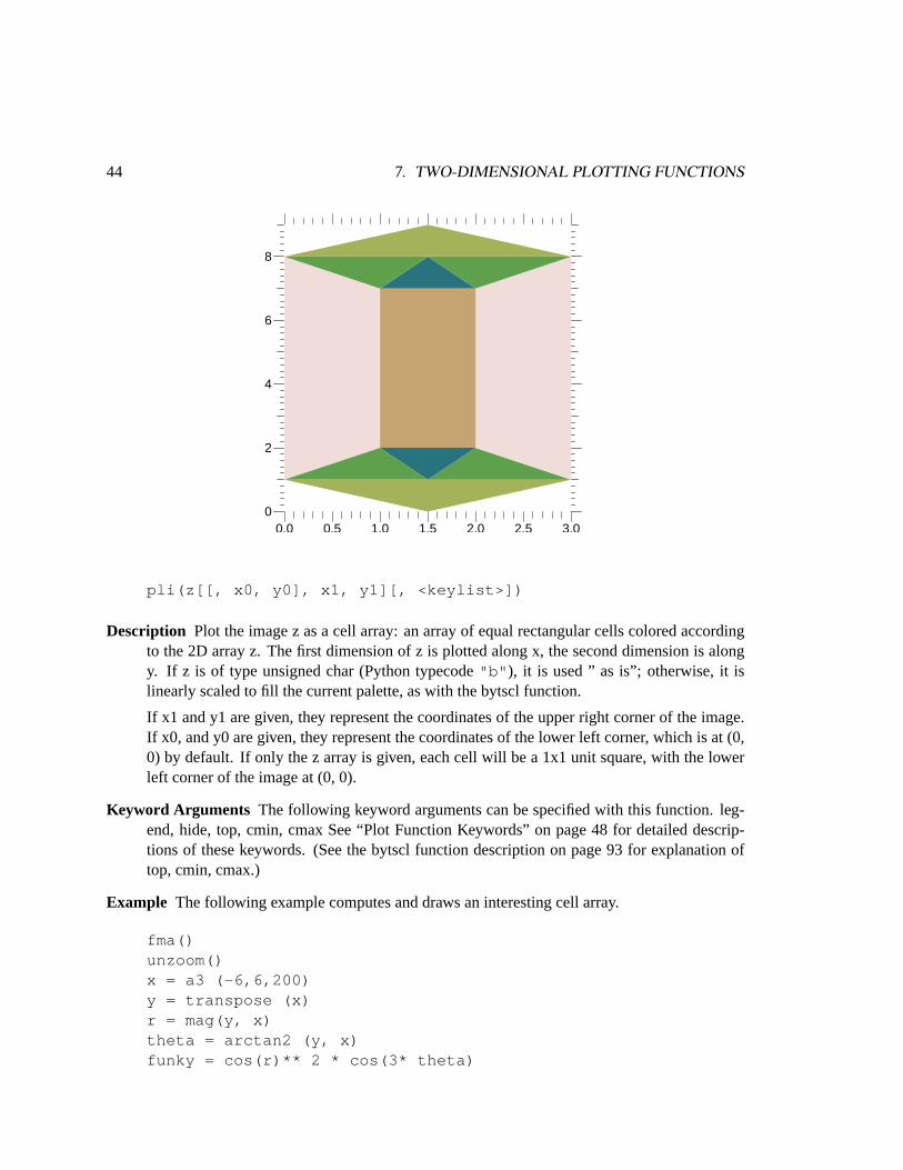
Description Plot the image z as a cell array: an array of equal rectangular cells colored accordingto the 2D array z. The first dimension of z is plotted along x, the second dimension is alongy. If z is of type unsigned char (Python typecode"b" ), it is used ” as is”; otherwise, it islinearly scaled to fill the current palette, as with the bytscl function.

If x1 and y1 are given, they represent the coordinates of the upper right corner of the image.If x0, and y0 are given, they represent the coordinates of the lower left corner, which is at (0,0) by default. If only the z array is given, each cell will be a 1x1 unit square, with the lowerleft corner of the image at (0, 0).

Keyword Arguments The following keyword arguments can be specified with this function. leg-end, hide, top, cmin, cmax See “Plot Function Keywords” on page 48 for detailed descrip-tions of these keywords. (See the bytscl function description on page 93 for explanation oftop, cmin, cmax.)

Example The following example computes and draws an interesting cell array.

fma()unzoom()x = a3 (-6,6,200)y = transpose (x)r = mag(y, x)theta = arctan2 (y, x)funky = cos(r)** 2 * cos(3* theta)


pli(funky)

0 50 100 150 200 0

50

100

150

200

pli,

7.1.10 pldj: Plot Disjoint Lines

Calling Sequence...

pldj(x0, y0, x1, y1[, <keylist>])

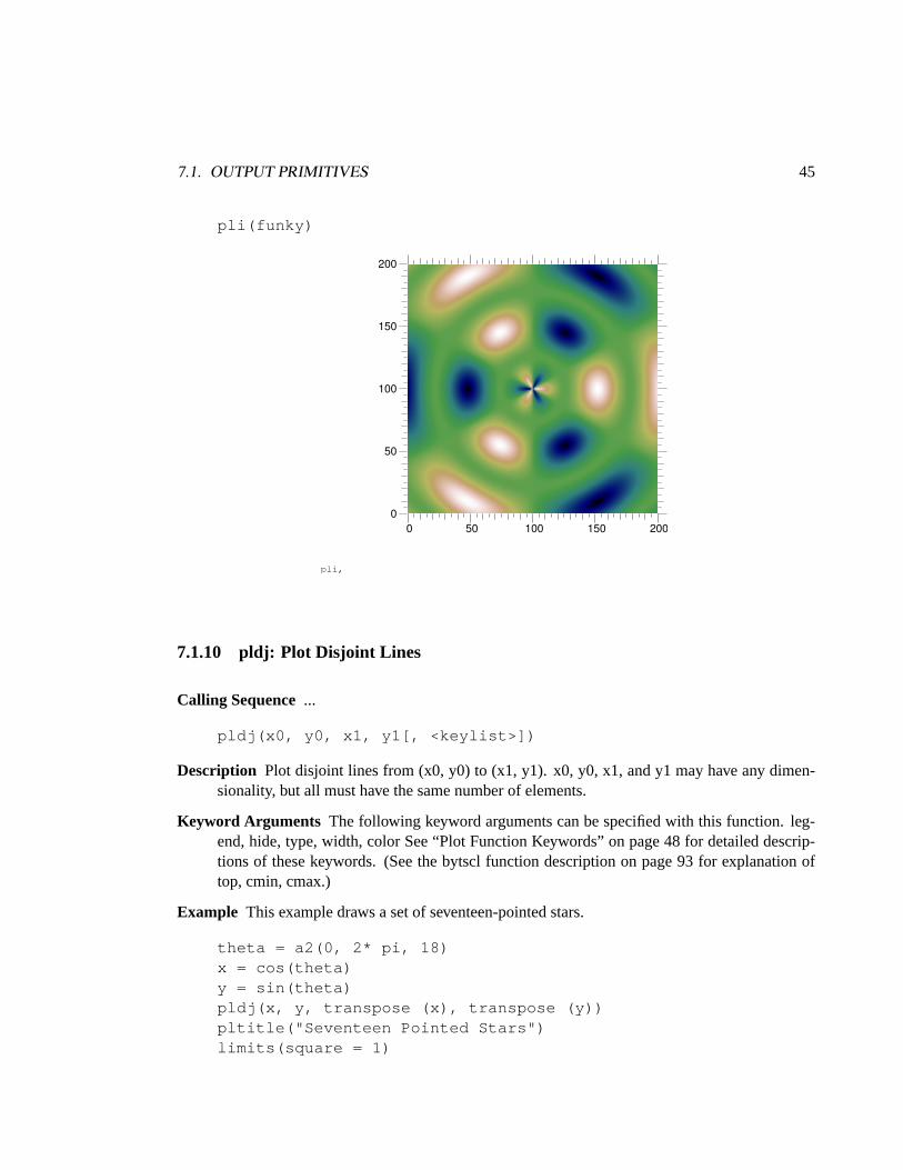
Description Plot disjoint lines from (x0, y0) to (x1, y1). x0, y0, x1, and y1 may have any dimen-sionality, but all must have the same number of elements.

Keyword Arguments The following keyword arguments can be specified with this function. leg-end, hide, type, width, color See “Plot Function Keywords” on page 48 for detailed descrip-tions of these keywords. (See the bytscl function description on page 93 for explanation oftop, cmin, cmax.)

Example This example draws a set of seventeen-pointed stars.

theta = a2(0, 2* pi, 18)x = cos(theta)y = sin(theta)pldj(x, y, transpose (x), transpose (y))pltitle("Seventeen Pointed Stars")limits(square = 1)


−1.0 −0.5 0.0 0.5

−0.5

0.0

0.5

Seventeen Pointed Stars

pldj,

7.1.11 plt: Plot Text

Calling Sequence...

plt(text, x, y[, <keylist>])

Description Plot text (a string) at the point (x, y). The exact relationship between the point (x, y)and the text is determined by the justify keyword. text may contain newline ("\n" ) charactersto output multiple lines of text with a single call.

The coordinates (x, y) are NDC coordinates (outside of any coordinate system) unless thetosys keyword is present and non-zero, in which case the text will be placed in the current co-ordinate system. However, the character height is never affected by the scale of the coordinatesystem to which the text belongs.

Note that the pledit command (see “pledit: Change Plotting Properties” on page 53) takes dxand/ or dy keywords to adjust the position of existing text elements.

Keyword Arguments The following keyword argument(s) apply only to this function. tosys =0/ 1 Establish the interpretation of (x, y). If tosys= 0 (the default), use Normalized DeviceCoordinates; if nonzero, use the current coordinate system.

font = <font value>height = <float value>opaque = 0/ 1


path = 0/ 1orient = <integer value>justify = (see text description)

Select text properties. The font can be any of the strings"courier" , "times" , "helvetica"(the default),"symbol" , or "schoolbook" . Append B for boldface and"I" for italic,so "courierB" is boldface Courier,"timesI" is Times italic, and"helveticaBI"is bold italic (oblique) Helvetica. Your X server should have the Adobe fonts (available freefrom the MIT X distribution tapes) for all these fonts, preferably at both 75 and 100 dpi.Occasionally, a PostScript printer will not be equipped for some fonts; often New CenturySchoolbook is missing. The font keyword may also be an integer: 0 is Courier, 4 is Times,8 is Helvetica, 12 is Symbol, 16 is New Century Schoolbook, and you add 1 to get boldfaceand/ or 2 to get italic (or oblique).

The height is the font size in points; 14.0 is the default. X windows only has 8, 10, 12, 14,18, and 24 point fonts, so don’t stray from these sizes if you want what you see on the screento be a reasonably close match to what will be printed. By default, opaque= 0 and text istransparent. Set opaque= 1 to white-out a box before drawing the text.

The default path (path= 0) is left-to-right text; set path= 1 for top-to-bottom text. The defaulttext justification,justify="NN" is normal in both the horizontal and vertical directions.Other possibilities are"L" , "C" , or "R" for the first character, meaning left, center, and righthorizontal justification, and"T" , "C" , "H" , "A" , or "B" for the second character, meaningtop, capline, half, baseline, and bottom vertical justification. The normal justification"NN"is equivalent to"LA" if path= 0, and to"CT" if path= 1. Common values are"LA" , "CA" ,and"RA" for garden variety left, center, and right justified text, with the y coordinate at thebaseline of the last line in the string presented to plt. The characters labeling the right axis ofa plot are"RH" , so that the y value of the text will match the y value of the correspondingtick. Similarly, the characters labeling the bottom axis of a plot are"CT" . The justificationmay also be a number, horizontal+ vertical, where horizontal is 0 for"N" , 1 for "L" , 2 for"C" , or 3 for "R" , and vertical is 0 for"N" , 4 for "T" , 8 for "C" , 12 for "H" , 16 for "A" ,or 20 for"B" .

The integer value orient (default 0) specifies one of four angles that the text makes with thehorizontal (0 is horizontal, 1 is ninety degrees, 2 is 180 degrees, and 3 is 270 degrees).

7.1.12 pltitle: Plot a Title

Calling Sequence...

pltitle(title)

Description Plot title centered above the coordinate system for any of the standard Gist styles. Youwill need to customize this for other plot styles.


7.1.13 plh: Plot a Histogram

Calling Sequence...

plh(y, [x, labels, <keylist>])

Description Draws a histogram, where the height of the bars is given by Y. If X is None, the barsin the histogram have a width equal to unity. If X is a single real number, it is interpreted asthe width of the bars. If X is a one- dimensional array with an equal number of elements asthe Y array, then X is interpreted as the widths of the bars. In all of these cases, the histogramstarts at the origin. However, if X is a one-dimensional array with one element more than Y,then X is interpreted as the locations of the start and end points of the bars in the histogram.If X is a one-dimensional array with twice as many elements as Y, then X represents the startand end points for each bar separately.

The keyword color is either a single color to fill the bars with, or a list of colors, one foreach bar. If the keyword labels is given, then the horizontal tick marks and numerical labelsare switched off. The keyword labels should then consist of a list of strings, with the samenumber of elements as Y. These labels are drawn below the horizontal axis.

To switch the tick marks and labels back on for subsequent plots, you can execute

window(style="work.gs")

which will reset the window to the usual work.gs style sheet.

Keyword Arguments width, hide, color

7.2 Plot Function Keywords

In addition to the keyword arguments described above with individual Gist primitive plotting com-mands, the following keywords are available to modify the details of the plots.

legend ...

legend = "text destined for the legend"

Set the legend for a plot. There are no default legends in PyGist. Legends are never plottedto the X window; use the plq command to see them interactively. Legends will appear inhardcopy output unless they have been explicitly turned off.

7.2. PLOT FUNCTION KEYWORDS 49

Plotting Commands: plg, plm, plc, plv, plf, pli, plt, pldj

See also:hide

hide ...

hide = 0/ 1

Set the visibility of a plotted element. The default is hide= 0, which means that the elementwill be visible. Use hide= 1 to remove the element from the plot (but not from the displaylist).

Plotting Commands: plg, plm, plc, plv, plf, pli, plt, pldj, plh

See also:legend

type ...

type = <line type value>

Select line type. Valid values are the strings"solid" , "dash" , "dot" , "dashdot" ,"dashdotdot" , and"none" . The"none" value causes the line to be plotted as a poly-marker. The type value may also be a number; 0 is"none" , 1 is"solid" , 2 is"dash" , 3is "dot" , 4 is "dashdot" , and 5 is"dashdotdot" .

Plotting Commands: plg, plm, plc, pldj

See also:width, color, marks, marker, rays, closed, smooth

width ...

width = <floating point value>

Select line width. Valid values are positive floating point numbers giving the line thicknessrelative to the default line width of one half point, which is width = 1.0.

Plotting Commands: plg, plm, plc, pldj, plv (only if hollow= 1), plh

See also:type, color, marks, marker, rays, closed, smooth

color ...

color = <color value>


Select line or text color. Valid values are the strings"bg" , "fg" , "black" , "white" ,"red" , "green" , "blue" , "cyan" , "magenta" , "yellow" , or a 0-origin index intothe current palette. The default is"fg" . Negative numbers may be used instead of the strings:-1 is "bg" (background), -2 is"fg" (foreground), -3 is black, -4 is white, -5 is red, -6 isgreen, -7 is blue, -8 is cyan, -9 is magenta, and -10 is yellow.

Plotting Commands: plg, plm, plc, pldj, plt, plh

See also:type, width, marks, marker, mcolor, rays, closed, smooth

marks ...

marks = 0/ 1

Select unadorned lines (marks= 0), or lines with occasional markers (marks= 1). Ignored iftype is "none" (indicating polymarkers instead of occasional markers). The spacing andphase of the occasional markers can be altered using the mspace and mphase keywords; thecharacter used to make the mark can be altered using the marker keyword.

Plotting Commands: plg, plc

See also:type, width, color, marker, rays, mspace, mphase, msize, mcolor

marker ...

marker = <character or integer value>

Select the character used for occasional markers along a polyline, or for the polymarker iftype="none" . The special values’\ 1’ , ’\ 2’ , ’\ 3’ , ’\ 4’ , and’\ 5’ stand forpoint, plus, asterisk, circle, and cross, which are prettier than text characters on output to somedevices. The default marker is the next available capital letter:’A’, ’B’, ..., ’Z’ .


See also:type, width, color, marks, rays, mspace, mphase, msize, mcolor

mspace ...

mspace = <float value>mphase = <float value>msize = <float value>

Select the spacing, phase, and size of occasional markers placed along polylines. The msizealso selects polymarker size if type is"none" . The spacing and phase are in NDC units (0.0013 NDC equals 1.0 point); the default mspace is 0.16, and the default mphase is 0.14, butmphase is automatically incremented for successive curves on a single plot. The msize is inrelative units, with the default msize of 1.0 representing 10 points.

7.2. PLOT FUNCTION KEYWORDS 51


See also:type, width, color, marks, marker, rays

mcolor ...

mcolor = <color value>

The mcolor keyword is the same as the color keyword, but controls the marker color insteadof the line color. Setting the color automatically sets the mcolor to the same value, so youonly need to use mcolor if you want the markers for a curve to be a different color than thecurve itself.



rays ...

rays = 0/ 1

Select unadorned lines (rays= 0), or lines with occasional ray arrows (rays= 1). Ignored iftype is"none" . The spacing and phase of the occasional arrows can be altered using therspace and rphase keywords; the shape of the arrowhead can be modified using the arrowwand arrowl keywords.


See also:type, width, color, marker, marks, rspace, rphase, arroww, arrowl

closed/smooth...

closed = 0/ 1smooth = 0/ 1/ 2/ 3/ 4

Select closed curves (closed= 1) or default open curves (closed= 0), or Bezier smoothing(smooth¿ 0) or default piecewise linear curves (smooth= 0). The value of smooth can be 1, 2,3, or 4 to get successively more smoothing. Only the Bezier control points are plotted to anX window; the actual Bezier curves will show up in PostScript hardcopy files. Closed curvesjoin correctly, which becomes more noticeable for wide lines; non-solid closed curves maylook bad because the dashing pattern may be incommensurate with the length of the curve.

Plotting Commands: plg, plc (smooth only)



region ...

region = <region number>

Select the part of mesh to consider. The region should match one of the numbers in theireg array. Putting region= 0 (the default) means to plot the entire mesh; that is, everythingEXCEPT region zero (non-existent zones). Any other number means to plot only the specifiedregion number; region= 3 would plot region 3 only.

Plotting Commands: plm, plc, plv, plf

8 Inquiry and Miscellaneous Functions

This chapter describes functions that are available to inquire about the state of PyGist control vari-ables and set their values. It also describes other miscellaneous functions.

8.1 Inquiry and Editing Functions

8.1.1 plq: Query Plot Element Status

Calling Sequence...

plq()legend_list = plq() **** RETURN VALUE NOT YET IMPLEMENTED ****plq(n_element[, n_contour])properties = plq(n_element[, n_contour])

Description Called as a subroutine, plq prints the list of legends for the current coordinate sys-tem (with an(H) to mark hidden elements), or prints a list of current properties of elementn_element (such as line type, width, font, etc.), or of contour numbern_contour ofelement numbern_element (which must be contours generated using the plc command).Elements and contours are both numbered starting with one; hidden elements or contours areincluded in this numbering.

The plq function always operates on the current coordinate system in the current graphicswindow; use window and plsys to change these.

8.1.2 pledit: Change Plotting Properties

Calling Sequence...

pledit([n_element[, n_contour],] <keylist>)

where, as usual,<keylist> has the formkey1=value1 , key2=value2 , ...

53

54 8. INQUIRY AND MISCELLANEOUS FUNCTIONS

Description pledit changes some property or properties of element numbern_element (and con-tour numbern_contour of that element). Ifn_element andn_contour are omitted,the default is the most recently added element, or the element specified in the most recent plqquery command.

The keywords can be any of the keywords that apply to the current element. These are: plg:color, type, width, marks, mcolor, marker, msize, mspace, mphase, rays, rspace, rphase, ar-rowl, arroww, closed, smooth plm: region, boundary, inhibit, color, type, width plc: region,color, type, width, marks, mcolor, marker, msize, mspace, mphase, smooth, levs (For con-tours, if you aren’t talking about a particularn_contour , any changes will affect ALL thecontours.) plv: region, color, hollow, width, aspect, scale plf: region pldj: color, type, widthplt: color, font, height, path, justify, opaque

A plv (vector field) element can also take the scalem keyword to multiply all vector lengthsby a specified factor.

A plt (text) element can also take the dx and/ or dy keywords to adjust the text position by(dx, dy).

8.1.3 plremove: Remove Plot Element from Display

Calling Sequence...

plremove(n_element)

Description Removes the element numbern_element from the display. Ifn_element is omit-ted, the default is the most recently added element, or the element specified in the most recentplq query command.

8.1.4 pldefault: Set Default Values

Calling Sequence...

pldefault(key1= value1, key2= value2, ...)

Description Set default values for the various properties of graphical elements. The keywords canbe most of the keywords that can be passed to the plotting commands:

plg: color, type, width, marks, mcolor, msize, mspace,mphase, rays, rspace, rphase, arrowl, arroww

plm: color, type, width

8.2. MISCELLANEOUS FUNCTIONS 55

plc: color, type, width, marks, mcolor, marker, msize,mspace, mphase

plv: color, hollow, width, aspectplf: edges, ecolor, ewidthpldj: color, type, widthplt: color, font, height, path, justify, opaque

The initial default values are:

color="fg", type="solid", width= 1.0 (1/ 2 point),marks= 1, mcolor="fg", msize= 1.0 (10 points), mspace= 0.16,mphase= 0.14,rays= 0, arrowl= 1.0 (10 points), arroww= 1.0 (4 points), rspace= 0.13,rphase= 0.11375,font="helvetica", height= 12.0, path= 0, justify="NN",opaque= 0,hollow= 0, aspect= 0.125,edges= 0, ecolor="fg", ewidth= 1.0 (1/ 2 point)

Additional default keywords are:

dpi, style, legends (see window command)palette (to set default filename as in palette command)maxcolors (default 200)cgmfilesize (default 10 MB) in units of MBytes

8.2 Miscellaneous Functions

8.2.1 bytscl: Convert to Color Array

Calling Sequence...

bytscl(z[, top= max_byte][, cmin= lower_cutoff][, cmax= upper_cutoff])

Description bytscl returns an unsigned char array of the same shape as z, with values linearlyscaled to the range 0 to one less than the current palette size. Ifmax_byte is specified, thescaled values will run from 0 tomax_byte instead.

If lower_cutoff and/ orupper_cutoff are specified, z values outside this range aremapped to the cutoff value; otherwise the linear scaling maps the extreme values of z to 0 andmax_byte .


8.2.2 histeqscale: Histogram Equalized Scaling

**** NOT YET IMPLEMENTED ****

Calling Sequence...

histeq_scale(z[, top= top_value][, cmin= cmin][, cmax= cmax])

Description histeq_scale returns a byte-scaled version of the array z having the property thateach byte occurs with equal frequency (z is histogram equalized). The result bytes range from0 to top_value , which defaults to one less than the size of the current palette (or 255 if nopli, plf, or palette command has yet been issued).

If non-nil cmin and/or cmax is supplied, values of z beyond these cutoffs are not included inthe frequency counts.

8.2.3 meshloc: Get Mesh Location

Calling Sequence...

mesh_loc(y0, x0[, y, x[, ireg]])

Description mesh_loc returns the zone index (= i+ imax*(j-1)) of the zone of the mesh (x, y)(with optional region number array ireg) containing the point (x0, y0). If (x0, y0) lies outsidethe mesh, returns 0. For example,ireg(mesh_loc(x0,y0,y,x,ireg)) is the regionnumber of the region containing (x0, y0). If no mesh specified, uses default. x0 and y0 maybe arrays as long as they are conformable.

8.2.4 mouse: Handle Mouse Click

This function is useful in developing interactive graphics applications.

Calling Sequence...

result = mouse(system, style, prompt)

Description mouse displays the specified prompt, then waits for a mouse button to be pressed, thenreleased. It returns a tuple of length eleven:

8.2. MISCELLANEOUS FUNCTIONS 57

result = [x_pressed, y_pressed, x_released, y_released,xndc_pressed, yndc_pressed, xndc_released,yndc_released, system, button, modifiers]

If system>=0 , the first four coordinate values will be relative to that coordinate system. Forsystem<0 , the first four coordinate values will be relative to the coordinate system underthe mouse when the button was pressed.

The second four coordinates are always normalized device coordinates, which start at (0, 0) inthe lower left corner of the 8.5x11 sheet of paper the picture will be printed on, with 0.0013NDC unit being 1/ 72.27 inch (1. 0 point). Look in the style sheet for the location of theviewport in NDC coordinates (see the style keyword).

If style is 0, there will be no visual cues that the mouse command has been called; this isintended for a simple click. If style is 1, a rubber band box will be drawn; if style is 2, arubber band line will be drawn. These disappear when the button is released.

Clicking a second button before releasing the first cancels the mouse function, which willthen return nil. Ordinary text input also cancels the mouse function, which again returns nil.

The left button reverses foreground for background (by XOR) in order to draw the rubberband (if any). The middle and right buttons use other masks, in case the rubber band is notvisible with the left button.

result[8] is the coordinate system in which the first four coordinates are to be interpreted.result[9] is the button which was pressed, 1 for left, 2 for middle, and 3 for right (4 and 5 arealso possible).

result[10] is a mask representing the modifier keys which were pressed during the operation:1 for shift, 2 for shift lock, 4 for control, 8 for mod1 (alt or meta), 16 for mod2, 32 for mod3,64 for mod4, and 128 for mod5.

8.2.5 moush: Mouse in a Mesh

Calling Sequence...

moush([y,x[,ireg]])

Description moush returns the 1-origin zone index for the point clicked in for the default mesh, orfor the mesh (x, y) (region array ireg).

8.2.6 pause: Pause

Calling Sequence...


pause(milliseconds)

Description Pause for the specified number of milliseconds of wall clock time, or until input arrivesfrom the keyboard. This is intended for use in creating animated sequences.

9 Three-Dimensional Plotting Functions

The PyGist 3D graphics uses the PyGist 2D graphics to draw its pictures; most of the 3D routinesare computational, and take 3D data in one form or another and massage it until, when plotted,it will appear to be a correct two-dimensional projection of a three-dimensional graph. The usualorder of operation in 3D PyGist is

• Retrieve or compute your data;

• Tell PyGist orientation and lighting information;

• Call the appropriate PyGist computational routines;

• Call one or more PyGist 3D plotting routines;

• Call the master function draw3, which actually displays the graph.

PyGist builds a list of information about the graph which you wish to plot, but in its normaloperating mode, does not actually draw the graph until you ask it to do so, by invoking draw3.Meanwhile, it stores the information about the graph in a Python list. In this chapter we shalldescribe the contents of this list in general terms, and the commands which you use to build it(orientation and lighting functions); the setup functions for complicated 3D plots; and the plottingfunctions themselves. In a final section, for people who may some day be maintaining or adding tothis code, we describe the auxiliary functions which everyday users will seldom if ever use.

9.1 Setting Up For 3D Graphics

9.1.1 The Plotting List

The 3D PyGist graphics keeps an internal list called_draw3_list containing complete informa-tion about the currently active frame (which may or may not be visible depending on whether draw3has been invoked). Regular users should never need to access this list; however, there is an accessfunction available calledget_draw3_list_ which code developers and maintainers may use toget at the list;get_draw3_n_ returns the number of elements in the viewing and lighting portionof the list, described below. Likewise, ordinary users do not really need to know the structure of thislist in detail; however, every user of the 3D graphics should be aware of the contents of the list, howit affects the graph, and what functions to use to alter it.

59

60 9. THREE-DIMENSIONAL PLOTTING FUNCTIONS

_draw3_list is a Python list, organized as follows:

[rotation, origin, camera_dist, ambient, diffuse, specular,spower, sdir, fnc 1 , args 1 , fnc 2 , args 2 ,...]

The elements of this list are divided into the viewing transformation, lighting specifications, anddisplay information, as follows:

Viewing: rotation: a 3-by-3 rotation matrix giving the angles of view. origin: a 3-vector givingthe coordinates of the origin in the user’s coordinate system.

camera dist: A real number giving the camera distance; the value None (the default) trans-lates to infinity.

Lighting: ambient: a light level (in arbitrary units) that is added to every part of the surface re-gardless of its orientation. It might be said to be the amount of light which a surfaceexudes on its own. A surface with ambient of 0 is totally black unless illuminated. dif-fuse: a light level which is proportional to cos( theta), where theta is the angle betweenthe surface normal and the viewing direction, so that surfaces directly facing the viewerare bright, while surfaces viewed edge on are unlit (and surfaces facing away, if drawn,are shaded as if they faced the viewer). specular: a light level proportional to a highpower spower of 1 + cos (alpha), where alpha is the angle between the specular reflec-tion angle and the viewing direction. The light source for the calculation of alpha liesin the direction sdir (a 3 element vector) in the viewer’s coordinate system at infinitedistance. You can have ns light sources by making specular, spower, and sdir (or anycombination) be vectors of length ns (3-by-ns in the case of sdir).

Display: fnc1, fnc2, etc.: Plotting function( s) (whose argument lists are arg 1 , arg 2 , etc., re-spectively) defining the component( s) of this graph. During its normal operating mode,the 3D graphics accumulates information about calls to plotting functions until the usercalls the function draw3. These calls are then executed when draw3 is invoked.

9.1.2 Functions For Setting Viewing Parameters

Angular orientation


orient3 (phi = angle 1 , theta = angle 2 )rot3 (xa = angle x , ya = angle y , za = angle z )

9.1. SETTING UP FOR 3D GRAPHICS 61

Description Note that most of the functions in 3D PyGist accept keyword arguments. These argu-ments may be entered in any order; omitted arguments will default to a sensible value.

orient3 sets the orientation of the object to (angle 1 , angle 2 ). Orientations are a subset ofthe possible rotation matrices in which the z axis of the object appears vertical on the screen(that is, the object z axis projects onto the viewer y axis). The theta angle is the angle fromthe viewer y axis to the object z axis, positive if the object z axis is tilted towards you (towardviewer +z). phi is zero when the object x axis coincides with the viewer x axis. If neitherphi nor theta is specified, phi defaults to -pi / 4 and theta defaults to pi / 6. If only phi isspecified, theta remains unchanged, unless the current theta is near pi / 2, in which case thetareturns to pi / 6, or unless the current orientation does not have a vertical z axis, in which casetheta returns to its default. If only theta is specified, phi retains its current value. Unlike rot3,orient3 is not a cumulative operation.

rot3 rotates the current 3D plot by angle x about viewer’s x axis, angle y about viewer’s yaxis, and angle z about viewer’s z-axis.

Physical orientation


mov3 (xa = val 1 , ya = val 2 , za = val 3 )aim3 (xa = val 1 , ya = val 2 , za = val 3 )setz3 (zc = dist)

Description mov3 moves the current 3D plot by val 1 along the viewer’s x axis, val 2 along theviewer’s y axis, and val 3 along the viewer’s z axis. aim3 moves the current 3D plot to putthe point (val 1 , val 2 , val 3 ) in object coordinates at the point (0, 0, 0)—the aim point—inthe viewer’s coordinates. In both functions, if any of the val 1 , val 2 , or val 3 is missing, itdefaults to 0.

setz3 sets the camera position to dist (x = y = 0) in the viewer’s coordinate system. If distis None or if zc is missing, set the camera to infinity (default).

9.1.3 Lighting Parameters

Calling Sequence...

light3 (ambient= a_level, diffuse= d_level, specular= s_level,spower= n, sdir= xyz)

This function is used to set the lighting parameters for the current drawing list.


9.1.4 Display List


<plot function> (arg 1 , arg 2 , arg 3 , ...)clear3 ( )

When one of the plotting functions (plwf, pl3surf, pl3tree) is called and the internal variable_draw3 has been set to zero, or else if it is nonzero and the idler is a do-nothing routine,Then this plot call will add<plot function> to the display list, and will process thearguments into a Python list, which will be added to the display list after the function name.

The function clear3 clears the display list of all plotting functions. It leaves orientation andlighting information unchanged.

9.2 3D Graphics Control Functions

9.2.1 Getting a Window

Calling Sequence...

window3 ( [n] [, dump = val] [, hcp = filename])

Description If n is specified, make window n the active window (open a window if necessary). Ifn is not specified, connect to the active window, or open one if none is active. Associate thehardopy file named filename with the window if hcp is specified; this will be postscript if thename ends in .ps, or cgm if it ends in .cgm. The style sheet associated with the window willbenobox. gs , i. e., a plain window with no axes (except possibly a gnomon). The dumpkeyword, if 1, causes the color palette to be dumped to the hcp file with each frame that issent there (otherwise hardcopy plots will be in greyscale).

9.2.2 Displaying the Gnomon

Webster’s defines a gnomon as “an object that by its position... serves as an indicator.” In 3D PyGist,the gnomon is a small diagram of the coordinate axes that appears in the lower left corner of a 3Dplot, if this capability has been turned on.

Calling Sequence...

9.2. 3D GRAPHICS CONTROL FUNCTIONS 63

gnomon ( [onoff] [, chr = <labels>] )set_default_gnomon ( [onoff])

Description gnomon toggles the gnomon display if onoff is omitted. If onoff is present and non-zero turn on the gnomon. If zero, turn it off.set_default_gnomon allows the user tospecify what the default gnomon is to be when the default idler is called (see the discussionin “The variable_draw3 and the idler” on page 64, and “The Default Idler” on page 64.)

The gnomon shows the x, y, and z axis directions in the object coordinate system. The direc-tions are labeled. The labels default to X, Y, and Z, but may be specified to be something elseby using the keyword chr. ¡labels¿ must be a Python list consisting of three character strings.The gnomon is always infinitely far behind the object (away from the camera).

There is a mirror-through-the-screen-plane ambiguity in the display which is resolved in twoways: (1) the (x, y, z) coordinate system is right-handed, and (2) If the tip of an axis projectsinto the screen, its label is drawn in opposite polarity to the other text in the screen.

9.2.3 Plotting the Display List

The only way that the display list can be plotted is by an invocation of the function draw3. The usermay control when this function gets called. To have a new plot appear totally under user control, set_draw3 to 0 (i. e., executeset_draw3_(0) ) and then call draw3 only when you want the plotto appear. To have a plot appear automatically after each plot command is given,_draw3 shouldbe set to 1 and the idler should be set to some function which calls draw3. The details are in “Thevariable_draw3 and the idler” on page 64.

Calling Sequence...

[lims = ] draw3 ( [called_as_idler = <val>])limits (lims [0], lims [1], lims [2], lims [3])

Description The functiondraw3 traverses the display list and executes each function on the listwith the list of arguments supplied. Assuming that the list is not empty, this means thatthe frame specified by this list will be displayed. If the parametercalled_as_idler ispresent and is nonzero, then afma (frame advance) call will be made first, meaning that thecurrent display will be erased before the new one is plotted. Otherwise the new display willappear on top of the old.

draw3 always attempts to return a list of four items[xmin, xmax, ymin, ymax]which give the maximum and minimum of the x and y coordinates actually plotted to thePyGist window. Calling the limits function with these four values as limits will scale thegraph properly. One could also perform computations with these limits (for example, to force


x and y to the same scale, or to shrink the graph a little to force it well inside the borders ofthe window). If you like the way your graphs look, then there is no reason to deal with thesenumbers.

We apologize for this messy kludge; we have encountered timing problems and other diffi-culties with the Gist limits calculating process which we have not been able to solve exceptby computing our own limits.

9.2.4 The variable draw3 and the idler

_draw3 is an internal 3D PyGist variable accessible to the user only by means of the access func-tions described below._draw3 , in conjunction with a function called an idler, determines whether,after a plot function and its arguments have been placed on the display list, some further actiontakes place. The default idler (see below) will cause the graph to be plotted each time it is called;and it will be called immediately after the plot function has been added to the display list, provided_draw3 is nonzero.


set_draw3_ (n)n = get_draw3_ ( )

Description The first function is used to set_draw3 to n (default 0), and the second, to read itscurrent setting.


clear_idler ( )set_idler (func_name)set_default_idler ( )call_idler ( )

Description The functionclear_idler sets the idler function to a routine which does nothing.It will be called after each plot function adds to the display list (if_draw3 is nonzero),but will do nothing. set_idler allows the user to define an action for 3D PyGist to takeafter each plot function call adds to the display list.func_name must be callable with noarguments. It will be called only if_draw3 is nonzero.set_default_idler will set theidler to call the function whose code is given below.call_idler gives you the capabilityto call the idler yourself, if you wish.

The Default Idler

Below is the code for the default idler.

9.3. DATA SETUP FUNCTIONS FOR PLOTTING 65

def _draw3_idler ( ) :global _default_gnomonorient3 ()if current_window () == -1 :window3 (0)else :window3 (current_window ())gnomon (_default_gnomon)lims = draw3 (1)if lims == None :returnelse :limits (lims [0], lims [1], lims [2], lims [3])

9.3 Data Setup Functions for Plotting

9.3.1 Creating a Plane

Calling Sequence...

plane3 (< normal>, <point>)

Description This function returns the coefficients of the equation of a plane as a vector of lengthfour. This is the form of a plane argument as expected by the slicing functions. ¡normal¿ isa vector of length three giving the direction numbers of the normal to the plane; ¡point¿ is avector of length three giving the coordinates of a point in the plane.

9.3.2 Creating a mesh3 argument

The function mesh3 is used to create a mesh3 object from your data. A mesh3 object is required asan input to a number of routines, most importantly, the various slicing functions.

Calling Sequence...

mesh3 (x, y, z)mesh3 (x, y, z, funcs = [f1, f2, ...], [verts = <spec>])


Description mesh3 creates a mesh3 object as expected by the various functions slice3, xyz3, getv3,etc. The form of a mesh3 object will be described below (See “Description of a mesh3 object”on page 65). Note that Python is able to determine which of the above calls is intendedbecause it can check for the presence of optional and keyword arguments and can check thedimensions and types of the arguments.

In the first two forms of the call, x, y, and z are coordinate arrays specifying the mesh. If x,y, and z are three dimensional of the same shape, then they represent the coordinates of thevertices of a regular rectangular mesh. If x, y, and z are one dimensional of the same size,then the keyword argument verts determines how they are interpreted. If verts is not present,then we have a structured rectangular mesh with unequally spaced nodes. If verts is present,then they represent the coordinates of an unstructured mesh, and the keyword argument vertsmust be used to pass information about the cells to the mesh3 function. ¡spec¿ can be either asingle two dimensional array of integer subscripts into x, y, and z, or a Python list of up to foursuch objects, one for each type of cell in the mesh. The format of the two dimensional arrayfor each type of cell shape is as follows: hexahedra: the array is no_hex_cells b y 8.The first subscript is the hexahedron cell number; for each value of this subscript, the secondindexes the vertices in canonical order (the first side in outward normal order, the oppositeside’s corresponding vertices in inward normal order).

prisms: the array is no_prism_cells b y 6. The first subscript is the prism cell number;for each value of this subscript, the second indexes the vertices in canonical order (thefirst side in outward normal order, the opposite side’s corresponding vertices in inwardnormal order).

pyramids: the array isno_pyr_cells by 5. The first subscript is the pyramid cell number;for each value of this subscript, the second indexes first the apex, then the vertices of thebase in inward normal order.

tetrahedra: the array isno_tet_cells by 4. The first subscript is the tetrahedron cellnumber; for each value of this subscript, the second indexes first some arbitrary cell asthe apex, then the vertices of the base in inward normal order. Each type of cell has arelative cell number running from 0 tono_celltype_cells -1. The cells are alsoassumed to have absolute cell numbers, which depend on the order in which the definingarrays appear, but will run consecutively starting from 0 in the first cell of the first typeup to the total number of cells -1 for the last cell of the last type.

The optional keyword funcs defines f1, f2, etc., which are arrays of function values (e. g.density, temperature) defined on the mesh. In the case of a regular (or structured) rectangularmesh, these functions are 3D arrays. If they represent cell-centered data, they will have oneless value along each dimension than the coordinate arrays. If they are vertex-centered data,then they will have the same dimensions. In the case of an unstructured mesh, f1, f2, etc.are one-dimensional arrays. If they represent cell-centered data, then they are indexed by theabsolute cell number, and must be the same length as the number of cells. If they represent

9.3. DATA SETUP FUNCTIONS FOR PLOTTING 67

vertex-centered data, then they are indexed the same as the vertices, and must be the samelength as the vertex arrays.

Calling Sequence...

mesh3 (xyz, funcs = [f1, f2, ...])

Description In this case xyz is a four dimensional array specifying the mesh; xyz [0] is the threedimensional x coordinate, xyz [1] is the three dimensional y coordinate, and xyz [2] is thethree dimensional z coordinate. (mesh3 actually converts the x, y, z arguments of the first twocalls into this xyz form in a mesh3 object; see “Description of a mesh3 object” on page 65.The funcs keyword operates as previously described.

Calling Sequence...

mesh3 (nxnynz, dxdydz, x0y0z0, funcs = [f1, f2, ...])

Description nxnynz is a vector of 3 integers, specifying the number of cells of a uniform 3D meshin the x, y, and z directions, respectively. dxdydz is an array of three reals, specifying the sizeof the entire mesh, not the size of one cell, in each of the three directions, and x0y0z0 is anarray of three reals, representing the point of minimum x, y, and z where the mesh begins.The funcs keyword operates as previously described.

Description of a mesh3 object The form of a mesh3 object varies according to whether the meshspecified was uniform, structured, or unstructured.

Uniform case, node equally spaced:...

[[ xyz3_unif, getv3_rect, getc3_rect, iterator3_rect],[ (nxnynz [0], nxnynz [1], nxnynz [2]),array ( [dxdydz, x0y0z0])], [f1, f2, ...]]

The four items in the first list are the names of functions. The details of these need notconcern us at this time except in their broad outlines. The iterator3 function will splitthe mesh into chunks for processing by the slicing functions, if necessary, in order tosave space. xyz3 returns the vertex coordinates of a chunk. getv3 returns the vertexvalues of a function on the chunk; getc3 returns cell values. Because these routinesnecessarily differ depending on the type of mesh, their names are passed along with themesh specifications to that the appropriate ones can be called. The remainder of theitems in the object specify the mesh and the function( s) defined on the mesh (if any; ifthere are none, the final list will be []).

Uniform case, nodes unequally spaced:...


[[ xyz3_unif, getv3_rect, getc3_rect, iterator3_rect],[ (len (x) -1, len (y) -1, len (z) -1),array ( [x, y, z])], [f1, f2, ...]]

The functions’ purpose is as described above. x, y, and z are one-dimensional arrays,possibly of different lengths, specifying the node coordinates of a uniform rectangularmesh, which might be unequally spaced. The triple consisting of the three array lengthsminus one gives the size of the mesh in cells.

Structured case: ...

[[ xyz3_rect, getv3_rect, getc3_rect, iterator3_rect],[dim_cell, xyz], [f1, f2, ...]]

The functions’ purpose is as described above.dim_cell is an integer vector of lengththree giving the size of the mesh in cells,dim_cell[0] being the x direction size,dim_cell[1] the y, anddim_cell[2] the z. xyz is a four-dimensional array ofcoordinates;xyz[0] is the three dimensional x coordinate array,xyz[1] is the threedimensional y coordinate array, andxyz[2] is the three dimensional z coordinate array.

Unstructured case: ...

[[ xyz3_irreg, getv3_irreg, getc3_irreg, iterator3_irreg],[dims, array ( [x, y, z]), sizes, totals], [f1, f2, ...]]

The functions’ purpose is as described above. dims is the value of the keyword argumentverts, i. e., it represents one array, or a list of up to four arrays, specifying the subscripts ofthe cell vertices into arrays x, y, and z in canonical order. If there is only one type of cellin the unstructured mesh, then sizes and totals will not be present; otherwise, they are usedto help recover the absolute cell number from a cell’s index in the list of cells of the sametype. sizes [i] is the number of cells of type i; totals [i] is the total number of cells up to andincluding type i.

9.4 The Slicing Functions

The slicing functions must be called in order to create data appropriate for the pl3surf (plot a 3Dsurface) and pl3tree (add a plot to a tree) routines. In general, the slicing routines take a meshspecification of some sort and return a list of the form

[nverts, xyzverts, color]

which specifies a set of polygonal cells and how to color them.

9.4. THE SLICING FUNCTIONS 69

nverts is no_cells long and the i th entry tells how many vertices the i th cell has.

xyzverts is sum (nverts) by 3 and gives the vertex coordinates of the cells in order, i. e., the firstnverts[0] entries inxyzverts are the coordinates of the first polygon’s vertices, thenextnverts[1] entries are the coordinates of the second polygon’s vertices, etc.

color , if present, isno_cells long and contains a color value for each cell in the mesh.

9.4.1 slice3mesh: Pseudo-slice for a surface

The function slice3mesh is designed specifically to produce an input argument for pl3surf, althoughif you want more than one surface in a picture, it can also be fed to pl3tree. It has several distinctcalling sequences, which Python can distinguish with its type savvy.

Calling Sequence...

slice3mesh (z [, color])

Description z is a two dimensional array of function values, assumed to be on a uniform meshnx by ny cells (assuming z is nx by ny) nx being the number of cells in the x direction, nythe number in the y direction. color, if specified, is either an nx by ny array of cell-centeredvalues by which the surface is to be colored, or an nx+1 by ny+1 array of vertex-centeredvalues, which will be averaged over each cell to give cell-centered values.

Calling Sequence...

slice3mesh (nxny, dxdy, x0y0, z [, color])

Description In this case, slice3mesh accepts the specification for a regular 2D mesh: nxny is thenumber of cells in the x direction and the y direction;x0y0 are the initial values of x and y;and dxdy are the increments in the two directions. z is the height of a surface above the xyplane and must be dimensioned nx + 1 by ny + 1. color, if specified, is as above.

Calling Sequence...

slice3mesh (x, y, z [, color])

Description z is as above, an nx by ny array of function values on a mesh of the same dimensions.There are two choices for x and y: they can both be one-dimensional, dimensioned nx and nyrespectively, in which case they represent a mesh whose edges are parallel to the axes; or elsethey can both be nx by ny, in which case they represent a general quadrilateral mesh.


9.4.2 slice3: Plane and Isosurface Slices of a 3D mesh

Calling Sequence...

[nverts, xyzverts, color] = \slice3 (m3, fslice, nv, xyzv [, fcolor [, flg 1 ]]

[, value = <val>] [, node = flg 2 ])

Description Slice the 3D mesh m3 as specified by fslice, returning the list [nverts, xyzverts, color].nverts is the number of vertices in each polygon of the slice, and xyzverts is the 3-by-sum(nverts) list of polygon vertices. If the fcolor argument is present, the values of that coloringfunction on the polygons are returned as the value of color. color will have the same size asnverts, i. e., the number of polygons in the slice, except that the keyword argument node,if present and nonzero, is a signal to return node-centered values rather than cell-centeredvalues. In the latter case color will be sum (nverts) long and entries in color will be associatedwith the corresponding coordinates in xyzverts. nv and xyzv are not needed; None should bepassed as their values (this is a leftover from an older version of the code).

fslice can be a function, a vector of 4 reals, or an integer number. If fslice is a function, itshould be of the form:

def fslice (m3, chunk)or, in the case of an isosurface slice,def fslice (m3, chunk, iso_index, _value)or for a plane slice,def fslice (m3, chunk, normal, projection)

and should return a list of function values on the specified chunk of the mesh m3. Moduleslice3 offers plane and isosurface slicers (for descriptions, see page 70). If you wish to writeyour own slice routine, you should bear in mind that the format of chunk depends on the typeof m3 mesh, so you should use only the appropriate mesh functions xyz3 and getv3 whichtake that type of m3 and chunk as arguments. The return value of fslice should have thesame dimensions as the return value of getv3; the return value of xyz3 has an additional firstdimension of length 3.

If fslice is a list of 4 reals, it is taken as a slicing plane as returned by plane3.

If fslice is a single integer, the slice will be an isosurface for the fslice th function associatedwith the mesh m3. In this case, the keyword value must also be present, representing thevalue of that function on the isosurface.

If fcolor is omitted or has value None, then slice3 returns None as the value of color.. If youwant to color the polygons in a manner that depends only on their vertex coordinates (e. g.,by a 3D shading calculation), use this mode.

9.4. THE SLICING FUNCTIONS 71

fcolor can be a function or a single integer. If fcolor is a function, it should be of the form: deffcolor (m3, cells, l, u, fsl, fsu, ihist) and should return a list of function values on the specifiedcells of the mesh m3. If the optional argument flg 1 after fcolor is not missing or None and isnon-zero, then the fcolor function is called with only two arguments:

def fcolor (m3, cells)

The cells argument will be the list of cell indices in m3 at which values are to be returned. l,u, fsl, fsu, and ihist are interpolation coefficients which can be used to interpolate from vertexcentered values to the required cell centered values, ignoring the cells argument. See getc3source code. The return values should always have the same size and shape as cells.

If fcolor is a single integer, then the slice will be an isosurface for the fcolor th variableassociated with the mesh m3.

9.4.3 slice2 and slice2x: Slicing Surfaces with planes

The functions slice2 and slice2x allow one to slice surfaces specified by slice3-type output. slice2will return the portion on one side of the slicing plane; slice2x will return both portions.


[nverts, xyzverts, values] = slice2 (plane, nv,xyzv, vals)[nverts, xyzverts, values, nvertb, xyzvertb, valueb] =slice2x (plane, nv, xyzv, vals)

Description The argument plane can be either a scalar or a plane3 (see “Creating a Plane” onpage 65); nv is an array of integers, the i th entry of which gives the number of verticesof the i-th polygonal cell;xyzv are the vertices of the coordinates of the cells, with eachconsecutive nv [i] entries representing the

vertices of the i th cell; and vals being a set of values as explained below. These argumentsare the same format as returned by slice3 and slice3mesh.

If plane is a plane3, then vals (if not None) is a cell-centered set of values expressing thecolor of each cell, and the outputs nverts, xyzverts, and values represent the polygons andtheir colors (if any) describing the portion of the sliced surface that is on the positive side ofthe plane. That’s all you get with slice2. With slice2x, you get in addition nvertb, xyzvertb,and valueb, which describe the part of the surface on the negative side of the slicing plane.Warning: one of these specifications could be None, None, None if the entire surface lies onone side of the plane.


If plane is a scalar value, then vals must be present and must be node-centered. In this case, theoutputs nverts, xyzverts, and values represent the polygons and their colors (if any) describingthe portion of the sliced surface where vals on the vertices are greater than or equal to thescalar value plane. (This actually allows you to form an arbitrary two-dimensional slice of asurface.) With slice2x, you get in addition nvertb, xyzvertb, and valueb, which describe thepart of the surface where vals on the vertices are less than the scalar value plane.

9.5 The 3D Plotting Functions

9.5.1 plwf: plot a wire frame

Calling Sequence...

plwf (z [, y, x] [, <keylist>] )

Description plwf plots a 3D wire frame of the given 2D array z. If x and y are given, then they mustbe the same shape as z or else len (x) should be the first dimension of z and len (y) the second.If x and y are not given, they default to the first and second indices of z, respectively. plwfcalls clear3 before putting the plot command on the display list, which means that PyGist canonly show one wire frame at a time using this function. (See pl3tree for graphs with multiplecomponents).

plwf accepts the following keyword arguments:

fill, shade, edges, ecolor, ewidth, cull, scale, cmax A description of the keywords follows:fill: optional colors to use (default is to make zones have background color), same dimensionoptions as for z argument to plf function, i. e., it should be the same dimension as the mesh(vertex-centered values) or one smaller in each dimension (cell-centered values).

shade: set non-zero to compute shading from the current 3D lighting sources.

edges: default is 1 (draw edges), but if you provide fill colors, you may set to 0 to suppressthe edges.

ecolor, ewidth: color and width of edges. cull: default is 1 (cull back surfaces), but if youwant to see the “underside” of the model, set to 0.

scale: by default, z is scaled to “reasonable” maximum and minimum values related to thescale of (x, y). This keyword alters the default scaling factor, in the sense that scale =2.0 will produce twice the z-relief of the default scale = 1.0.

cmax: the ambient keyword in light3 can be used to control how dark the darkest surface is;use this to control how light the lightest surface is. The lightwf routine can change thisparameter interactively.

9.5. THE 3D PLOTTING FUNCTIONS 73

Examples The following example computes the information for a surface with a peak and a valley,and then plots the resulting wire frame with various options. In the first case, we see simplyan opaque wire frame.

set_draw3_(0)x = span (-1, 1, 64, 64)y = transpose (x)z = (x + y) * exp (-6.*( x* x+ y* y))orient3 ( )light3 ( )plwf (z, y, x)[xmin, xmax, ymin, ymax] = draw3( 1)limits (xmin, xmax, ymin, ymax)plt(" opaque wire mesh", .30, .42)

Next, we see the same surface shaded from a default light source (roughly over the viewer’sright shoulder) and with the mesh lined in red.

plwf( z, y, x, shade= 1, ecolor=" red")[xmin, xmax, ymin, ymax] = draw3( 1)limits (xmin, xmax, ymin, ymax)

Finally, the following sequence plots the same surface with no edges, and with lighting com-ing from the back.

plwf( z, y, x, shade= 1, edges= 0)light3 ( diffuse=. 1, specular= 1., sdir= array([ 0,0,-1]))[xmin, xmax, ymin, ymax] = draw3( 1)limits (xmin, xmax, ymin, ymax)

9.5.2 pl3surf: plot a 3-D surface

Calling Sequence...

pl3surf (nverts, xyzverts [, values] [, <keylist>])

Description Perform simple 3D rendering of an object created by slice3 (possibly followed byslice2). nverts and xyzverts are polygon lists as returned by slice3, so xyzverts is sum (nverts)-by-3, where nverts is a list of the number of vertices in each polygon. If present, the valuesshould have the same length as nverts; they are used to color the polygon. If values is not


specified, the 3D lighting calculation set up using the light3 function will be carried out.Keywords cmin and cmax as for plf, pli, or plfp are also accepted. (If you do not supplyvalues, you probably want to use the ambient keyword to light3 instead of cmin here, butcmax may still be useful.)

pl3surf calls clear3 before putting the plot command on the display list, which means thatPyGist can only show one surface at a time using this function. (See pl3tree below for graphswith multiple components).

Example The following example is the familiar sombrero function. The first few lines of codecompute its value.

nc1 = 100nv1 = nc1 + 1br = -(nc1 / 2)tr = nc1 / 2 + 1x = arange (br, tr, typecode = Float) * 40. / nc1y = arange (br, tr, typecode = Float) * 40. / nc1z = zeros ( (nv1, nv1), Float)r = sqrt (add. outer ( x ** 2, y ** 2)) + 1e-6z = sin (r) / r

In order to use pl3surf, we need to construct a mesh using mesh3. The way we shall do thatis to define a function on the 3d mesh so that the sombrero function is its 0-isosurface.

z0 = min (ravel (z))z0 = z0 -.05 * abs (z0)maxz = max (ravel (z))maxz = maxz + .05 * abs (maxz)zmult = max (max (abs (x)), max (abs (y)))dz = (maxz -z0)nxnynz = array ( [nc1, nc1, 1], Int)dxdydz = array ( [1.0, 1.0, zmult* dz], Float )x0y0z0 = array ( [float (br), float (br), z0* zmult], Float )meshf = zeros ( (nv1, nv1, 2), Float )meshf [:, :, 0] = zmult* z -(x0y0z0 [2])meshf [:, :, 1] = zmult* z -(x0y0z0 [2] + dxdydz [2])

Finally, we create the mesh and call the plotting functions.

m3 = mesh3 (nxnynz, dxdydz, x0y0z0, funcs = [meshf])fma ()# Make sure we don’t draw till ready


set_draw3_(0)pldefault( edges= 0)[nv, xyzv, col] = slice3 (m3, 1, None, None, value = 0.)orient3 () # (default orientation)pl3surf (nv, xyzv)lim = draw3 (1)dif = 0.5 * (lim [3] -lim [2])# dif is used to compress the y scale a bit.limits (lim [0], lim [1], lim [2] -dif, lim [3] + dif)palette (" gray. gp")

The graph that results from this sequence of code is on the next page. This next sequence offunctions uses slice3mesh to draw the same surface; this time the polygons that make up thesurface are colored according to height (using the rainbow palette).

# Try new slicing function to get color graph[nv, xyzv, col] = slice3mesh (nxnynz [0: 2], dxdydz [0: 2],x0y0z0 [0: 2], zmult * z, color = zmult * z)pl3surf (nv, xyzv, values = col)lim = draw3 (1)dif = 0.5 * (lim [3] -lim [2])limits (lim [0], lim [1], lim [2] -dif, lim [3] + dif)palette (" rainbow. gp")

9.5.3 pl3tree: add a surface to a plotting tree

pl3tree accepts surfaces and slices of surfaces in the slice2/ slice3 format, and, as its name suggests,builds a b-tree. Its purpose is to attempt to analyze multiple surface plots in such a way as todetermine the order of plotting, so that hidden portions of the surfaces will be graphed first, and thiscovered by later portions. pl3tree may be called multiple times to build plots of arbitrary complexity.

Calling Sequence...

pl3tree (nverts, xyzverts [, values] [, <keylist>])

Description pl3tree accepts the following keywords: plane, cmin, cmax, split pl3tree adds thepolygon list specified by nverts (number of vertices in each polygon) and xyzverts (3-by-sum(nverts) vertex coordinates) to the currently displayed b-tree. If values is specified, it musthave the same dimension as nverts, and represents the color of each polygon. If values is notspecified, then the polygons are assumed to form an isosurface which will be shaded by the


current 3D lighting model; the isosurfaces are at the leaves of he b-tree, sliced by all of theplanes. If plane (in the format returned by a call to plane3) is specified, then the xyzvertsmust all lie in that plane, and that plane becomes a new slicing plane in the b-tree.

Each leaf of the b-tree consists of a set of sliced isosurfaces. A node of the b-tree consists ofsome polygons in one of the planes, a b-tree or leaf entirely on one side of that plane, and ab-tree or leaf on the other side. The first plane you add becomes the root node, slicing anyexisting leaf in half. When you add an isosurface, it propagates down the tree, getting slicedat each node, until its pieces reach the existing leaves, to which they are added. When youadd a plane, it also propagates down the tree, getting sliced at each node, until its pieces reachthe leaves, which it slices, becoming the nodes closest to the leaves.

This structure is relatively easy to plot, since from any viewpoint, a node can always be plottedin the order from one side, then the plane, then the other side.

If keyword split is set nonzero (the default), then this routine assumes a “split palette”; thecurrent palette will be “split” or truncated so that its colors are numbered 0 to 99, while colors100 to 199 will be greyscale. Colors for the values will be scaled to fit from color 0 to color99, while the colors from the shading calculation will be scaled to fit from color 100 to color199. (If values is specified as an unsigned char array (Python typecode “b”), however, it willbe used without scaling.) You may specify a cmin or cmax keyword to affect the scaling;cmin is ignored if values is not specified (use the ambient keyword from light3 for that case).

Example In the following example, nx, ny, and nz are each 20. First we compute the mesh andsome data on the mesh.

xyz = zeros ( (3, nx, ny, nz), Float)xyz [0] = multiply. outer ( span (-1, 1, nx),ones ( (ny, nz), Float))xyz [1] = multiply. outer ( ones (nx, Float),multiply. outer ( span (-1, 1, ny),ones (nz, Float)))xyz [2] = multiply. outer ( ones ( (nx, ny), Float),span (-1, 1, nz))r = sqrt (xyz [0] ** 2 + xyz [1] ** 2 + xyz [2] ** 2)theta = arccos (xyz [2] / r)phi = arctan2 (xyz [1] , xyz [0] + logical_not (r))y32 = sin (theta) ** 2 * cos (theta) * cos (2 * phi)m3 = mesh3 (xyz, funcs = [r * (1. + y32)])

Next we construct two isosurfaces, an inner (function value .5) and an outer (function value1.0) using slice3.

[nv, xyzv, dum] = slice3 (m3, 1, None, None, value = .50)


# (inner isosurface)[nw, xyzw, dum] = slice3 (m3, 1, None, None, value = 1.)# (outer isosurface)

Now we create two planes, use one to form a plane slice through the mesh, then the second toslice the first in half.

pxy = plane3 ( array ([ 0, 0, 1], Float ), zeros (3, Float))pyz = plane3 ( array ([ 1, 0, 0], Float ), zeros (3, Float))[np, xyzp, vp] = slice3 (m3, pyz, None, None, 1)# (pseudo-colored plane slice)[np, xyzp, vp] = slice2 (pxy, np, xyzp, vp)# (cut slice in half)

Finally, we slice each isosurface in half, keeping both halves (slice2x calls), then slice the“top” half of each in half again, discarding the front of each (slice2 calls).

[nv, xyzv, d1, nvb, xyzvb, d2] = \slice2x (pxy, nv, xyzv, None)[nv, xyzv, d1] = slice2 (-pyz, nv, xyzv, None)# (... halve one of those halves)[nw, xyzw, d1, nwb, xyzwb, d2] = \slice2x ( pxy , nw, xyzw, None)# (split outer in halves)[nw, xyzw, d1] = slice2 (-pyz, nw, xyzw, None)

Now, a sequence of calls to pl3tree sets up the graph, and a call todemo5_light actuallyplots it. For completeness, we give the functiondemo5_light first.

making_movie = 0def demo5_light (i) :global making_movieif i >= 30 : return 0theta = pi / 4 + (i -1) * 2 * pi/ 29light3 (sdir = array ( [cos( theta), .25, sin( theta)],Float))draw3 ( not making_movie )return 1fma ()split_palette (" earth. gp")gnomon (1)


clear3 ()# Make sure we don’t draw till readyset_draw3_(0)pl3tree (np, xyzp, vp, pyz)pl3tree (nvb, xyzvb)pl3tree (nwb, xyzwb)pl3tree (nv, xyzv)pl3tree (nw, xyzw)orient3 ()light3 (diffuse = .2, specular = 1)limits (square= 1)demo5_light (1)

9.6 Contour Plotting on Surfaces: plzcont and pl4cont

Contour lines can be plotted on a surface, or filled contours can be drawn, or both, by means of thetwo functions plzcont (plot z contours, i. e., contours according to height in the z direction) andpl4cont (plot 4D contours, i. e., contours determined by some other function defined on the surface.


plzcont (nverts, xyzverts, contours = 8, scale = "lin",clear = 1, edges = 0, color = None, cmin = None,cmax = None, zaxis_min = None, zaxis_max = 0, split = 0)pl4cont (nverts, xyzverts, values, contours = 8, scale ="lin", clear = 1, edges = 0, color = None, cmin = None,cmax = None, caxis_min = None, caxis_max = 0, split = 0)

Description plzcont plots z contours, and pl4cont plots contours derived from the function val-ues. nverts and xyzverts specify the polygons which define the surface. nverts is an array ofintegers,

the i th entry of which gives the number of vertices of the i th polygonal cell; xyzverts are thevertices of the coordinates of the cells, with each consecutive nv [i] entries representing thevertices

of the i-th cell; and values (for pl4cont) being a set of values, one for each vertex. Thesearguments are the same format as returned by slice3 and slice3mesh ( see Section “slice3:Plane and Isosurface Slices of a 3D mesh” on page 70). plzcont and pl4cont actually dorepeated calls to slice2x (see Section “slice2 and slice2x: Slicing Surfaces with planes” onpage 71) in order to obtain the contour curves.

9.6. CONTOUR PLOTTING ON SURFACES: PLZCONT AND PL4CONT 79

Keyword Arguments contours can be one of the following: N, an integer: Plot N contours (there-fore, N+ 1 colored components of the surface) CVALS, a vector of floats: draw thecontours at the specified levels.

scale can be"lin" , "log" , or "normal" specifying the contour scale. (Only applicableif contours = N, of course).

clear If clear == 1 , clear the display list first. Otherwise the current contour plot will beadded to the display list.

edges If edges == 1 , plot the edges.

color If color == None , then bytscl the palette into N + 1 colors and send each of theslices to pl3tree with the appropriate color. Ifcolor=="bg" , will plot only the edges.See also split (below).

cmin, cmax If cmin is given, use it instead of the minimum c actually being plotted inthe computation of contour levels. Ifcmax is given, use it instead of the maximumc actually being plotted in the computation of contour levels. This is done so that acomponent of a larger graph will have the same colors at the same levels as every othercomponent, rather than its levels being based on its own maximum and minimum, whichmay lie inside or outside those of the rest of the graph.

zaxis min, zaxis max zaxis_min andzaxis_max represent axis limits on z as expressedby the user. If present,zaxis_min will inhibit plotting of all lesser z values, andzaxis_max will inhibit the plotting of all greater z values.

caxis min, caxis max caxis_min andcaxis_max represent axis limits on c as expressedby the user. If present,caxis_min will inhibit plotting of all lesser c values, andcaxis_max will inhibit the plotting of all greater c values.

split If split == 1, then it is intended to plot this portion of the graph as if the palette has beensplit, so only colors 0-99 will be used to color the contours. If split == 0, then all colorsfrom 0 to 199 will be used.

Example In the following example, we compute the sombrero function and then use plzcont todraw it with contours in"normal" scale. In"normal" scale, the top and bottom contoursare two standard deviations away from the mean. Thus the peak of the sombrero is all thesame color because its few points contribute very little to the standard deviation.

# compute sombrero functionx = arange (-20, 21, typecode = Float)y = arange (-20, 21, typecode = Float)z = zeros ( (41, 41), Float)r = sqrt (add. outer ( x ** 2, y ** 2)) + 1e-6z = sin (r) / rfma ()clear3 ()


gnomon (0)# Make sure we don’t draw till readyset_draw3_(0)palette (" rainbow. gp")[nv, xyzv, dum] = slice3mesh (x, y, z)plzcont (nv, xyzv, contours = 20, scale = "normal")[xmin, xmax, ymin, ymax] = draw3 (1)limits (xmin, xmax, ymin, ymax)

To draw the same function in"lin" scale, with edges visible, enter the following code:

plzcont (nv, xyzv, contours = 20, scale = "lin", edges= 1)[xmin, xmax, ymin, ymax] = draw3 (1)limits (xmin, xmax, ymin, ymax)

9.7 Animation: movie and spin3

9.7.1 The movie module and function

Calling Sequence...

movie (draw_frame [, time_limit = 120.][, min_interframe = 0.0][, bracket_time = array ([ 2., 2.], Float )][, lims = None][, timing = 0])

Description Note: All but the first argument are keyword arguments, with defaults as shown. Thisfunction runs a movie based on the givendraw_frame function. The movie stops after atotal elapsed time oftime_limit seconds, which defaults to 60 (one minute), or when thedraw_frame function returns zero. (N. B. Currently the timing option described here andin a subsequent paragraph is not completely implemented.)

draw_frame is a function described as follows:def draw_frame (i) :# Input argument i is the frame number.# draw_frame should return non-zero if there are more# frames in this movie. A zero return will stop the# movie.

9.7. ANIMATION: MOVIE AND SPIN3 81

# draw_frame must NOT include any fma command if the# making_movie variable is set (movie sets this variable# before calling draw_frame)

If min_interframe is specified, a pause will be added as necessary to slow down themovie.min_interframe is a time in seconds (default 0). The keywordbracket_time(again a time in seconds) can be used to adjust the duration of the pauses after the first andlast frames. It may also be a two element array [beg, end]. If the pause at the end is greaterthan five seconds, you will be prompted to explain that hitting ¡RETURN¿ will abort the finalpause. (Well, the Python version does not currently have this capability due to the difficultyof implementing it consistently over various platforms.)

timing = 1 enables a timing printout for your movie. If every frame of your movie has thesame limits, use the lims keyword argument to fix the limits during the movie.

Example In the following example, the movie demonstrates the effect of a moving light source onthe currently drawn surface. (The plot functions creating the surface have not been shown; itis assumed that the data for the surface is on the current display list.)

Thedraw_frame function is as follows:

def demo5_light (i) :global making_movieif i >= 30 : return 0theta = pi / 4 + (i -1) * 2 * pi/ 29light3 (sdir =array ( [cos( theta), .25, sin( theta)], Float))# without an explicit call to draw3, the light3# function would cause no changes until Python# paused for input from the keyboard, since# unlike the primitive plotting functions (plg, plf,# plfp, ...) the fma call made by the movie function# will not trigger the 3-D display list. any movie# frame display function which uses the 3-D drawing# functions in pl3d. py will need to do this. the# !making_movie flag supresses the fma in draw3 if# this function is called by movie (which issues# its own fma), but allows it otherwisedraw3 ( not making_movie )return 1

Here is the Python code necessary to run a movie. This particular animation shows the surfacewith a peak and valley which we saw earlier in this chapter ( See “Examples” on page 73),with a moving light source. A few frames of the movie are shown on the next page.


set_draw3_(0)x = span (-1, 1, 64, 64)y = transpose (x)z = (x + y) * exp (-6.*( x* x+ y* y))orient3 ( )light3 (diffuse=. 2, specular= 1 )limits_( square = 1)plwf (z, y, x, shade= 1, edges= 0)[xmin, xmax, ymin, ymax] = draw3 (1)limits (xmin, xmax, ymin, ymax)making_movie = 1movie( demo5_light, lims = [xmin, xmax, ymin, ymax])making_movie = 0

9.7.2 The spin3 function

spin3 is a function which takes an existing 3D plot and spins it about an axis. It actually calls moviefor you, with adraw_frame function which is internal to the pl3d module and not availableoutside this module, because its name begins with an underscore.

Calling Sequence...

spin3 (nframes = 30,axis = array ([-1, 1, 0], Float),tlimit = 60.,dtmin = 0.0,bracket_time = array ([ 2., 2.], Float),lims = None,timing = 0,angle = 2. * pi)

Description Spin the current 3D display list about axis (default[-1,1,0] ) over nframes (default30). Note that all arguments are keywords. Also note that the timing keywords are allowedbut are not currently implemented. Their meanings are:

tlimit: the total time allowed for the movie in seconds (default 60).

dtmin: the minimum allowed interframe time in seconds (default 0.0).

bracket time: (as for movie function in movie.py).

lims: the axis limits, if you wish to specify them. timing = 1 if you want timing measuredand printed out, 0 if not.

9.8. SYNTACTIC SUGAR: SOME HELPFUL FUNCTIONS 83

angle: the total angle about the axis through which the object will be rotated. During eachstep of the rotation, the object will rotate angle / (nframes-1).

Example In this example, we take the surface discussed previously (see “Example” on page 81)and rotate it about an axis. Assume that the sequence of code given there has been executed,giving the figure shown there. Then we do the following to run the movie:

spin3 () # (lims = [l0, l1, l2, l3])

Four frames from the resulting movie are shown on the next page.

TABLE 2. Frames from Movie of Rotating Isosurfaces

9.8 Syntactic Sugar: Some Helpful Functions

9.8.1 Specifying the palette to be split: splitpalette

Calling Sequence...

split_palette ( [palette_name])

Description Split the current palette (ifpalette_name is not present) or the specified palette (ifpalette_name is present) into two parts; colors 0 to 99 will be a compressed version ofthe original, while colors 100 to 199 will be a gray scale. For details on the available palettes,see “palette: Set or Retrieve Palette” on page 27.

If you usesplit_palette to split the palette yourself, then be sure to call pl3tree withkeyword split = 0, because otherwise pl3tree will split it again, with bizarre results. Alterna-tively, you can use the palette function referenced above to set the palette to your choice, thencall pl3tree with split = 1.

9.8.2 Saving and restoring the view and lighting: save3, restore3


view = save3 ()movie (_spin3, ... <other arguments>)restore3 (view)


Description In the above, thesave3 function returns a copy of the current 3D viewing trans-formation and lighting, so that the user can put it aside in the variable view. The_spin3function does actually change the viewing transformation and lighting; the call to restore3with argument view sets it back to its previous configuration.

References

[1] Lee Busby, Fred Fritsch, and Zane Motteler, “Manual 4, Chapter 1: The Python GraphicsInterface,” UCRL-MA-128569, November 23, 1998.

85

10 Acknowledgements

The following people contributed to the PyGist development over the years:

• Lee Busby(LLNL) wrote the original extension wrapping Gist for use from Python (gistCmodule.c ).Work was based on Yorick 1.3.

• Zane Motteler (retired LLNL) was responsible for the object-oriented component of theoriginal Python Graphics (PyGraph), EZPlot, and the Narcisse module (all three are no longerin use). Wrote much of the documentation external to documentation contributed from SteveLanger and Dave Munro for their software. Also maintained the entire graphics interface(PyGraph) until retirement.

• Fred Fritsch (retired LLNL) developed the template for the documentation and contributedto some of the original PyGraph documentation.

• Dave Munro (LLNL), author of Yorick (and Gist). Also, identified the subset of Yorick1.5 required for PyGist. Helped identify the technical issues, particularly related to eventhandling, involved with interfacing Gist (1.5) to Python 2.x. Also contributes routinely bymaking Yorick changes to accommodate PyGist.

• Steve Langer(LLNL), Yorick developer. Collaborated with Munro on the interpreted 3Dgraphics. Also contributed to identification of issues in bringing up PyGist 1.3 to 1.5.

• Paul Dubois (LLNL) wrote the PDB and Ranf modules, and worked with Konrad Hinsen(Laboratoire de Dynamique Moleculaire, Institut de Biologie Structurale, Grenoble, France)and James Hugunin (Massachusetts Institute of Technology) on NumPy, the numeric exten-sion to Python, without which this work could not have been done.

• Michiel de Hoon (University of Tokyo, Human Genome Center) contributed solutions to theproblem of getting Python and Gist to work together in handling events. He rewrote the buildprocedure (setup.py) and was also responsible for the Cygwin port and collaborated withMunro on the Windows port to 1.5. Michiel also provided the Windows-related documenta-tion in this manual.

• Lila Chase (LLNL) currently maintains PyGist (2001-). Gathered relevant pieces from Py-Gist 1.3, upgraded to Yorick 1.5 and latest Python and Numeric, created new infrastructure,ported, and tested on a wide variety of platforms.

86

A Useful Functions for Developers

November 23, 1998

In this chapter we describe more of the available functions in detail, for those who are reallyinterested in plumbing the depths of the low-level 3D graphics.

A.1 Find 3D Lighting: get3 light

Calling Sequence...

get3_light(xyz [, nxyz])

Description Return 3D lighting for polygons with vertices XYZ. If NXYZ is specified, XYZshould be sum(nxyz)-by-3, with NXYZ being the list of numbers of vertices for each polygon(as for the plfp function; see page 42). If NXYZ is not specified, XYZ should be a quadri-lateral mesh, ni-by-nj-by-3 (as for the plf function; see page 40). In the first case, the returnvalue is len (NXYZ) long; in the second case, the return value is (ni-1)-by-(nj-1).

The parameters of the lighting calculation are set by the light3 function (see “Lighting Pa-rameters” on page 61).

A.2 Get Normals to Polygon Set: get3normal

Calling Sequence...

get3_normal(xyz [, nxyz])

Description Return 3D normals for polygons with vertices XYZ. If NXYZ is specified, XYZshould be sum(nxyz)-by-3, with NXYZ being the list of numbers of vertices for each polygon(as for the plfp function; see page 42). If NXYZ is not specified, XYZ should be a quadri-lateral mesh, ni-by-nj-by-3 (as for the plf function; see page 40). In the first case, the returnvalue is len(NXYZ)-by-3; in the second case, the return value is (ni-1)-by-(nj-1)-by-3.

The normals are constructed from the cross product of the lines joining the midpoints of twoedges which as nearly quarter the polygon as possible (the medians for a quadrilateral). Nocheck is made that these not be parallel; the returned “normal” is [0, 0, 0] in that case. Also,if the polygon vertices are not coplanar, the “normal” has no precisely definable meaning.

87

88 APPENDIX A. USEFUL FUNCTIONS FOR DEVELOPERS

A.3 Get Centroids of Polygon Set: get3centroid

Calling Sequence...

get3_centroid(xyz [, nxyz])

Description Return 3D centroids for polygons with vertices XYZ. If NXYZ is specified, XYZshould be sum(nxyz)-by-3, with NXYZ being the list of numbers of vertices for each polygon(as for the plfp function; see page 42). If NXYZ is not specified, XYZ should be a quadri-lateral mesh, ni-by-nj-by-3 (as for the plf function; see page 40). In the first case, the returnvalue is len(NXYZ) in length; in the second case, the return value is (ni-1)-by-(nj-1)-by-3.

The centroids are constructed as the mean value of all vertices of each polygon.

A.4 Get Viewer’s Coordinates: get3xy

Calling Sequence...

get3_xy(xyz [, 1])

Description Given 3-by-anything coordinates XYZ, return X and Y in viewer’s coordinate sys-tem (set by rot3, mov3, orient3, etc.; see “Functions For Setting Viewing Parameters” onpage 60). If the second argument is present and non-zero, also return Z (for use in sort3dor get3_light , for example; see “Sort z Coordinates: sort3d” on page 89 and “Find 3DLighting: get3light” on page 87.). If the camera position has been set to a finite distancewith setz3 (see “Physical orientation” on page 61), the returned coordinates will be tangentsof angles for a perspective drawing (and Z will be scaled by 1/zc). x, y, and z can be either1D or 2D, so this routine is written in two cases.

A.5 Add object to drawing list: set3 object

Calling Sequence...

set3_object(drawing_function, [arg1, arg2,...])

Description Set up to trigger a call to draw3, adding a call to the3D display list of the form:

DRAWING_FUNCTION ([ARG1, ARG2, ...]))

A.6. SORT Z COORDINATES: SORT3D 89

When draw3 callsDRAWING_FUNCTION, the external variabledraw3_ will be non-zero,soDRAWING_FUNCTIONcan be written like this:

def drawing_function(arg) : if (draw3_) :arg1=arg[0]arg1=arg[1]......< calls to get3_xy, sort3d, get3_light, etc.>......< calls to graphics functions plfp, plf, etc.>...return

...< verify args>...

...< do orientation and lighting independent calcs>...set3_object (drawing_function, [arg1, arg2,...])

A.6 Sort z Coordinates: sort3d

Calling Sequence...

sort3d(z, npolys)

Description Given Z and NPOLYS, with len(Z)== sum(npolys), return a 2-element list [LIST,VLIST] such that take(Z, VLIST) and take (NPOLYS, LIST) are sorted from smallest averageZ to largest average Z, where the averages are taken over the clusters of length NPOLYS.Within each cluster (polygon), the cyclic order of take (Z, VLIST) remains unchanged, butthe absolute order may change.

This sorting order produces correct or nearly correct order for a plfp call to make a plotinvolving hidden or partially hidden surfaces in three dimensions. It works best when thepolygons form a set of disjoint closed, convex surfaces, and when the surface normal changesonly very little between neighboring polygons. (If the latter condition holds, then even ifsort3d misorders two neighboring polygons, their colors will be very nearly the same, and themistake won’t be noticeable.) A truly correct 3D sorting routine is impossible, since theremay be no rendering order which produces correct surface hiding (some polygons may needto be split into pieces in order to do that). There are more nearly correct algorithms than this,but they are much slower.


A.7 Set the cmax parameter: lightwf

Calling Sequence...

lightwf (cmax)

Description Sets the cmax parameter interactively, assuming the current 3D display list containsthe result of a previous plwf call. This changes the color of the brightest surface in thepicture. The darkest surface color can be controlled using the ambient keyword to light3 (see“Lighting:” on page 61).

A.8 Return a Wire Frame Specification: xyz wf

Calling Sequence...

xyz_wf (z, [y, x] [, scale = 1.0])

Returns a 3-by-ni-by-nj array whose 0 th entry is x, 1 th entry is y, and 2 th entry is z. z isni-by-nj. x and y, if present, must be the same shape. If not present, integer ranges will beused to create an equally spaced coordinate grid in x and y. The function which scales the“topography” of z(x, y) is potentially useful apart from plwf.

For example, the xyz array used by plwf can be converted from a quadrilateral mesh plottedusing plf to a polygon list plotted using plfp like this:

Description xyz= xyz_wf(z, y, x, scale= scale)ni= z. shape[ 1]nj= z. shape[ 2]list = ravel (add. outer (ravel(add. outer (adders, zeros(nj-1, Int))) +arange((ni-1)*(nj-1), typecode = Int),array ([[ 0, 1], [nj + 1, nj]])))xyz= array([ take(ravel(xyz[ 0]), list),take(ravel(xyz[ 1]), list),take(ravel(xyz[ 2]), list)])nxyz= ones((ni-1)*(nj-1)) * 4;

The resulting array xyz is 3-by-(4*(nj-1)*(ni-1)). xyz[ 0: 3,4* i: 4*(i+ 1)] are the clockwisecoordinates of the vertices of cell number i.

A.9. CALCULATE CHUNKS OF MESH: ITERATOR3 91

A.9 Calculate Chunks of Mesh: iterator3


iterator3 (m3)iterator3 (m3, chunk, clist)iterator3_rect (m3)iterator3_rect (m3, chunk, clist)iterator3_irreg (m3)iterator3_irreg (m3, chunk, clist)

Description The iterator3 functions combine three distinct operations: 1. If only the M3 ar-gument is given, return the initial chunk of the mesh. The chunk will be no more thanchunk3_limit cells of the mesh.

2. If only M3 and CHUNK are given, return the next CHUNK, or None if there are no morechunks.

3. If M3, CHUNK, and CLIST are all specified, return the absolute cell index list correspond-ing to the index list CLIST of the cells in the CHUNK. Do not increment the chunk in thiscase.

The form of the CHUNK argument and return value for cases (1) and (2) is not specified, butit must be recognized by the xyz3 and getv3 functions (see “Return Vertex Coordinates for aChunk: xyz3” on page 94 and “Get Vertex Values of Function: getv3” on page 91) which goalong with this iterator3. (For case (3), CLIST and the return value are both ordinary indexlists.) In the irregular case, it is guaranteed that the returned chunk consists of only one typeof cell (tetrahedra, hexahedra, pyramids, or prisms).

A.10 Get Vertex Values of Function: getv3

Calling Sequence...

getv3(i, m3, chunk)getv3_rect(i, m3, chunk)getv3_irreg (i, m3, chunk)

Description getv3 returns vertex values of the I th function attached to 3D mesh M3 for cells inthe specified CHUNK. The CHUNK may be a list of cell indices, in which case getv3 returnsa 2x2x2x(CHUNK. shape) list of vertex coordinates. CHUNK may also be a mesh-specificdata structure used in the slice3 routine (see “slice3: Plane and Isosurface Slices of a 3D


mesh” on page 70), in which case getv3 may return a (ni) x(nj) x(nk) array of vertex values.For meshes which are logically rectangular or consist of several rectangular patches, this isup to 8 times less data, with a concomitant performance advantage. Use getv3 when writingslicing functions for slice3.

getv3_rect does the job for a regular rectangular mesh.getv3_irreg , for an irregularmesh, returns a 3-list whose elements are:

1. the function values for the I th function on the vertices of the given CHUNK. (Thefunction values must have the same dimension as the coordinates; there is no attempt toconvert zone-centered values to vertex-centered values.)

2. an array of relative cell numbers within the list of cells of this type.

3. a number that can be added to these relative numbers to give the absolute cell numbersfor correct access to their coordinates and function values

A.11 Get Cell Values of Function: getc3

Calling Sequence...

getc3(i, m3, chunk)getc3(i, m3, clist , l, u, fsl, fsu, cells)

Description Returns cell values of the I th function attached to 3D mesh M3 for cells in the spec-ified CHUNK. The CHUNK may be a list of cell indices, in which case getc3 returns a(CHUNK. shape) array of vertex coordinates. CHUNK may also be a mesh-specific datastructure used in the slice3 routine (see “slice3: Plane and Isosurface Slices of a 3D mesh” onpage 70), in which case getc3 may return a (ni) x(nj) x(nk) array of vertex values. There is nosavings in the amount of data for such a CHUNK, but the gather operation is cheaper than ageneral list of cell indices. Use getc3 when writing coloring functions for slice3.

If CHUNK is a CLIST, the additional arguments L, U, FSL, and FSU are vertex index listswhich override the CLIST if the I th attached function is defined on mesh vertices. L andU are index arrays into the (CLIST. shape) x2x2x2 vertex value array, say vva, and FSLand FSU are corresponding interpolation coefficients; the zone centered value is computedas a weighted average of involving these coefficients. The CELLS argument is required byhistogram to do the averaging. See the source code for details. By default, this conversion (ifnecessary) is done by averaging the eight vertex-centered values.

getc3_rect does the job for a regular rectangular mesh.getc3_irreg : Same thingasgetc3_rect , i. e., returns the same type of data structure, but from an irregular mesh.m3[1] is a 2-list; m3[1][0] is an array whose i th element is an array of coordinate indicesfor the i th cell, or a list of up to four such arrays. m3 [1] [1] is the 3 by nverts array of

A.12. CONTROLLING POINTS CLOSE TO THE SLICING PLANE: SLICE2 PRECISION 93

coordinates. m3 [2] is a list of arrays of vertex-centered or cell-centered data. chunk maybe a list, in which case chunk [0] is a 2-sequence representing a range of cell indices; or itmay be a one-dimensional array, in which case it is a nonconsecutive set of cell indices. It isguaranteed that all cells indexed by the chunk are the same type.

A.12 Controlling Points Close to the Slicing Plane: slice2precision


precision = get_slice2_precision ()set_slice2_precision (precision)

Description Internal variable_slice2_precision controls how slice2 (or slice2x) handlespoints very close to the slicing plane or surface. PRECISION should be a positive number orzero. Zero PRECISION means to clip exactly to the plane, with points exactly on the planeacting as if they were slightly on the side the normal points toward. Positive PRECISIONmeans that edges are clipped to parallel planes a distance PRECISION on either side of thegiven plane. (Polygons lying entirely between these planes are completely discarded.)

Default value is 0.0.

A.13 Scale variables to a palette: bytscl, splitbytscl

Calling Sequence...

bytscl(z, top= max_byte, cmin= lower_cutoff,cmax= upper_cutoff)split_bytscl (x, upper, cmin = None, cmax = None)

Description bytscl returns an unsigned char array (Python typecode"b" ) of the same shape asZ, with values linearly scaled to the range 0 to one less than the current palette size. IfMAX_BYTEis specified, then the scaled values will run from 0 toMAX_BYTEinstead. IfLOWER_CUTOFFand/ orUPPER_CUTOFFare specified, Z values outside this range aremapped to the cutoff value; otherwise the linear scaling maps the extreme values of Z to 0andMAX_BYTE.

split_bytscl is as the bytscl function, but scales to the lower half of a split palette (0-99,normally the color scale) if the second parameter is zero or nil, or the upper half (100-199,normally the gray scale) if the second parameter is non-zero.


A.14 Return Vertex Coordinates for a Chunk: xyz3

Calling Sequence...

xyz3 (m3, chunk)

Description Return vertex coordinates for CHUNK of 3D mesh M3. The CHUNK may be a listof cell indices, in which case xyz3 returns a (CHUNK. shape)) x3x2x2x2 list of vertex co-ordinates. CHUNK may also be a mesh-specific data structure used in the slice3 routine(see “slice3: Plane and Isosurface Slices of a 3D mesh” on page 70), in which case xyz3may return a 3x(ni) x(nj) x(nk) array of vertex coordinates. For meshes which are logicallyrectangular or consist of several rectangular patches, this is up to 8 times less data, with aconcomitant performance advantage. Use xyz3 when writing slicing functions or coloringfunctions for slice3.

A.15 Find Corner Indices of List of Cells: to corners3

Calling Sequence...

to_corners3(list, nj, nk)

Description Convert an array of cell indices in an (ni-1)-by-(NJ-1)-by-(NK-1) logically rectangulargrid of cells into the array of len(LIST)-by-2-by-2-by-2 cell corner indices in the correspond-ing ni-by-NJ-by-NK array of vertices. The algorithm used is described in section “Moreslice3 details”. Note that this computation in Yorick gives an absolute offset for each cellquantity in the grid. In Yorick it is legal to index a multidimensional array with an absoluteoffset. In Python it is not. However, an array can be flattened if necessary.

Other changes from Yorick were necessitated by row-major order and 0-origin indices, andof course the lack of Yorick array facilities.

A.16 Timing: timer , timer print


timer_ (elapsed)timer_ (elapsed, split)timer_print (label1, split1 [, label2, split2, ...])

A.16. TIMING: TIMER , TIMER PRINT 95

Description timer returns a triple consisting of the times [cpu, system, wall]. If argument split ispresent, a sequence is returned whose first element is [cpu, system, wall] and whose secondelement is the sum of split and the difference between the new and old values of ’elapsed. ’timer_print prints out a timing summary for splits accumulated by timer.

B Maintenance: Things You Really Didn’t Want to Know

In this chapter we discuss in even more gory detail how the PyGist graphics are put together.

B.1 The Workhorse: gistCmodule

The reader should be familiar with many of the functions in gistCmodule from the chapter “Two-Dimensional Plotting Functions” on page 33. Most of the gistCmodule functions discussed there,and many of the helper functions, are pretty close to literal translations of the equivalent functionsin Gist, the main difference being the superstructure built on top of them in order to handle PyOb-jects. In addition to the plotting functions, a number of functions in gistCmodule are essential formaintenance of that module, and are discussed here. We also discuss briefly a few other functionswhich are not literal translations of Gist functions.

B.1.1 Memory Maintenance: PyObjects

One of the primary challenges facing the developer of Python extensions is correct managementof the reference counting for Python objects. Memory leaks will result if the programmer fails todecrement the reference count in temporary objects. On the other hand, decrementing the refer-ence count too early can cause an object to go away that is referred to later, which can cause asegmentation fault when it is referenced. We have semi-automated the process in gistCmodule bymaintaining a list of all PyObjects created in the process of running one of the module’s functions.This list is declared as follows:

#define ARRAY_LIST_SIZE 30static PyObject * PyArrayList [ARRAY_LIST_SIZE];static int array_list_length = 0;

There is a suite of functions for manipulating PyArrayList.

Function Prototypes

static int addToArrayList (PyObject * obj)static void clearArrayList ()

96

B.1. THE WORKHORSE: GISTCMODULE 97

static void removeFromArrayList (PyObject * obj)static void takeOffArrayList (PyObject * obj)

addToArrayList places obj onPyArrayList and returns 1 if successful. If obj is NULLor the list is full, returns 0.clearArrayList DECREF’s everything on the list, and setsarray_list_lengthto 0. This needs to be done prior to any error return.removeFromArrayList DECREF’s obj (ifit is on the list), removes it from the list, and compresses the list.takeOffArrayList removesobj from the list and compresses the list, but does not DECREF obj. This is done, for example,when obj is to be returned to the caller.

addToArrayList occurs throughout gistCmodule primarily in macros which create arrays. All ofthese macros use the TRY macro, which is defined as follows:

#define TRY( e, m) do{ if(!( e)){ clearArrayList(); \clearFreeList( 0); clearMemList(); return m;}} while( 0)

The idea behind TRY is that generally Python functions return 0 or NULL if an error occurred.In this case it is necessary to get rid of all temporary objects and memory which was allocated up tothis point. clearArrayList was discussed above, clearFreeList and clearMemList are discussed laterin the chapter.

The array creation macros are as follows:

#define GET_ARR( ap, op, type, dim, cast) \TRY( addToArrayList(( PyObject *)( ap=( PyArrayObject *)\PyArray_ContiguousFromObject( op, type, dim, dim))), \(cast) PyErr_NoMemory ())

This macro is the usual protocol for creating a contiguous array from a PyObject which has beensent as an argument to a function.

#define NEW_ARR( ap, n, dims, type, cast) \TRY( addToArrayList(( PyObject *)( ap=\(PyArrayObject *) PyArray_FromDims( n, dims, type))), \(cast) PyErr_NoMemory ())

This macro is used usually when creating an array whose dimensions are known and which isto be filled with computed data.

98 APPENDIX B. MAINTENANCE: THINGS YOU REALLY DIDN’T WANT TO KNOW

#define RET_ARR( op, ndim, dim, type, data, cast)\TRY( addToArrayList( op=\PyArray_FromDimsAndData( ndim, dim, type, data)), \(cast) PyErr_NoMemory ())

This final macro is used when we have a block of data and we wish to create an array contain-ing this data, usually as a return value from a function. In order to keep this object from beingpermanent, use the following macro:

#define SET_OWN( op) \( (PyArrayObject *) op)-> flags |= OWN_DATA

This macro sets a flag in the PyObject which tells Python that it can be DECREF’ed.

B.1.2 Memory Management: ArrayObjects

Definition ArrayObjects are defined as follows:

typedef struct arrayobject {void * data ;int size ;char typecode ;} ArrayObject;

These objects are used primarily in the slice2 routines to store temporary results during thecalculation. The final results are passed back in PyArrayObjects created byRET_ARR. Twolists of ArrayObjects are maintained by the slice2 suite: list 0 by slice2 itself, and list 1, whichis used by_slice2_part , which is called byslice2 . These lists are declared as follows:

#define MAX_NO_LISTS 2#define MAX_LIST_SIZE 30

static ArrayObject * freeList [MAX_NO_LISTS] [MAX_LIST_SIZE];static int freeListLen [MAX_NO_LISTS] = {0, 0};

Function Prototypes ...


static ArrayObject * allocateArray (int size, char tc,int nlist)static ArrayObject * copyArray (ArrayObject * a)static ArrayObject * arrayFromPointer (int size, char tc,void * data, int nlist)static void freeArray (ArrayObject * a, int n)static void clearFreeList (int n)static int addToFreeList (ArrayObject * x, int n)static void removeArrayOnly (ArrayObject * x, int n)static void removeFromFreeList (ArrayObject * x, int n)

Description allocateArray allocates an appropriate amount of space for size items of type tc. Itthen creates an ArrayObject containing this data and puts it on freeList [nlist]. copyArraymakes and returns a copy of a. It does not add a to any freeList. arrayFromPointer createsan arrayObject whose data pointer points to data; it is assumed that the caller has suppliedcorrect size and tc arguments. The resulting object is placed on freeList [nlist]. freeArrayfrees a’s data and then a itself, and removes it from freeList [n] if it is there. clearFreeListfrees everything on freeList [n] and sets the list length to 0. addToFreeList adds x to freeList[n], if it can. removeArrayOnly removes the array from freeList [n], then frees x withoutfreeing its data. This would most likely be done whenRET_ARRcreates a PyArrayObjectwhich points to x’s data. removeFromFreeList frees x’s data, then x itself, and removes xfrom freeList [n].

B.1.3 Memory Management: naked memory

Occasionally in gistCmodule it is necessary to malloc a block of memory which is not containedinside some type of object.

Definition MemList is used to keep track of such memory:

#define MEM_LIST_SIZE 15

static void * PyMemList [MEM_LIST_SIZE];static int mem_list_length = 0;

MemList is maintained by its own suite of functions.

Function Prototypes static int addToMemList (void * addr)static void clearMemList ()

Description The first function adds an address to MemList; the second frees everything on Mem-List and sets its length back to 0.


B.1.4 Computing contour curves: contour

Calling Sequence...

# Set mesh firstplmesh (y, x, ireg, triangle = triangle)[nc, yc, xc] = contour (level, z)

Description The calling sequence given above emphasizes that mesh parameters should be set bya call to plmesh prior to calling contour. plmesh arguments are explained in section “plmesh:Set Default Mesh” on page 34. If level is a scalar floating point number, then the the returnedvalues are the points at that contour level. All such points lie on edges of the mesh. If acontour curve closes, the final point is the same as the initial point (i. e., that point is includedtwice in the returned list). If level is a sequence of two reals, then contour returns the pointsof a set of polygons which outline the regions between the two contour levels. The returnedvalues are in the form required for arguments of plfp (see Section “plfp: Plot a List of FilledPolygons” on page 42). These will include points on the mesh boundary which lie betweenthe levels, in addition to the edge points for both levels. The polygons are closed, simplyconnected, and will not contain more than about 4000 points (larger polygons are split intopieces with a few points repeated where the pieces join). The 2D filled contour plot routineplfc (see Section “plfc: Plot filled contours” on page 41) operates by calling contour with pairsof adjacent contour levels, and then calling plfp with the output and a single color, inside aloop. contour needed to be programmed in C because it can be called many times to do asingle filled contour plot, and the calculations take too long to be performed in interpretedcode. contour calls lower level Gist routines that do most of the work.

B.1.5 Computing slices: slice2, slice2x,slice2part

The 3D graphics in Gist itself is still experimental, and virtually all the computational functions arewritten in Yorick, an interpreted language. Many of the PyGist 3D computations were translatedinto Python from Yorick, originally including the slice2 and slice2x functions, and their auxiliary,_slice2_part . When we implemented contours and filled contours on surfaces (which is cur-rently not implemented in Gist itself), we used slice2 and slice2x to compute the contours andthe polygon lists enclosed within them. These computations were much too slow, so we rewroteslice2 in C (slice2x remains in Python; it just calls slice2 with a parameter set) and put them intothe gistCmodule. The user interface to these functions has been discussed in a previous section“slice2 and slice2x: Slicing Surfaces with planes”, but we discuss them here from the viewpoint ofimplementation. We also discuss the “hidden” function_slice2_part here for the first time.



[nverts, xyzverts, values] = slice2 (plane, nv,xyzv, vals = None, _slice2x = 0)[nverts, xyzverts, values, nvertb, xyzvertb, valueb] =slice2x (plane, nv, xyzv, vals)static int _slice2_part (ArrayObject * xyzc,ArrayObject * keep, ArrayObject * next, ArrayObject * dp,ArrayObject * prev, ArrayObject * last,ArrayObject * valc, ArrayObject ** xyzc_new,ArrayObject ** nvertc, ArrayObject ** valc_new,int freexyzc, int freevalc)

Description The argument plane can be either a scalar or a plane3 (see “Creating a Plane” onpage 65); nv is an array of integers, the i th entry of which gives the number of vertices of thei th polygonal cell;xyzv are the vertices of the coordinates of the cells, with each consecutivenv[i] entries representing the

vertices of the i-th cell; and vals being a set of values, one for each cell. These arguments arethe same format as returned by slice3 and slice3mesh.

If plane is a plane3, then vals (if not None) is a cell-centered set of values expressing thecolor of each cell, and the outputs nverts, xyzverts, and values represent the polygons andtheir colors (if any) describing the portion of the sliced surface that is on the positive side ofthe plane. That’s all you get with slice2. With slice2x, you get in addition nvertb, xyzvertb,and valueb, which describe the part of the surface on the negative side of the slicing plane.Warning: one of these specifications could be None, None, None if the entire surface lies onone side of the plane. If plane is a scalar value, then vals must be present and must be node-centered. In this case, the outputs nverts, xyzverts, and values represent the polygons andtheir colors (if any) describing the portion of the sliced surface where vals on the vertices aregreater than or equal to the scalar value plane. (This actually allows you to form an arbitrarytwo-dimensional slice of a surface.) With slice2x, you get in addition nvertb, xyzvertb, andvalueb, which describe the part of the surface where vals on the vertices are less than thescalar value plane.

The optional parameter_slice2x , if 1, tells slice2 to return slices on both sides of theslicing surface or plane; if not present, or 0, then the slice on “top” is returned. slice2 worksby deciding which polygons lie entirely “above” the slicing surface, which ones lie entirely“below” the slicing surface, and which ones are cut by the surface. If_slice2x is 0, then theones “below” the surface are discarded. slice2 then calls_slice2_part with the polygonsto be cut by the plane; once to get the cut polygons “above” the surface, then, if_slice2xis 1, a second time to get the cut polygons “below” the surface. The list of uncut and cutpolygons “above” the surface is concatenated and returned (_slice2x == 0 ); the list ofuncut and cut polygons “below” the surface is concatenated and returned also if_slice2xis 1.

In the case of a plane slice, suppose that the equation of the slicing plane is


ax + by + cz = d

Then a point(x1,y1,z1) is considered to be on the positive side of the plane if

ax 1 + by 1 + cz 1 -d >= _slice2_precision

and on the negative side if

ax 1 + by 1 + cz 1 -d < _slice2_precision

For a discussion of_slice2_precision , and how to get and set its value, see Section“Controlling Points Close to the Slicing Plane:slice2precision” on page 93.

In the case of a slicing surface, vertex i is considered to be above the surface if

vals [i] -plane >= _slice2_precision

and below it if

vals [i] -plane < _slice2_precision

For all intents and purposes, the user may assume that_slice2_precision is 0.0, as thisis the default. However, we allow you to change this if you think you have good reason.

There is a conceptual difficulty for the case of a quad face all four of whose edges are cutby the slicing plane or surface. This can only happen when two opposite corners are aboveand the other two below the slicing plane. There are three possible ways to connect the fourintersection points in two pairs: (1) // (2)and (3) X. There is a severe problem with (1) and (2) in that a consistent decision must bemade when connecting the points on the two cells which share the face—that is, each facemust carry information on which way it is triangulated. For a regular 3D mesh, it is relativelyeasy to come up with a consistent scheme for triangulating faces, but for a general unstruc-tured mesh, each face itself must carry this information. This presents a huge challenge fordata flow, which we don’t believe is worthwhile, because the X choice is unique, and we don’tsee why we shouldn’t use it here. For contouring routines, we reject the X choice on aestheticgrounds, and perhaps that will prove to be the case here as well but we believe we should trythe simple way out first. In this case, we are going to be filling these polygons with a colorrepresenting a function value in the cell. Since the adjacent cells should have nearly the samevalues, the X-traced polygons will have nearly the same color, and we doubt there will bean aesthetic problem. Anyway, our implementation of slice3, slice2, and_slice2_partproduces the unique X (bowtied) polygons, rather than attempting to choose between // or(non-bowtied) alternatives. Besides, in the case of contours, the trivial alternating triangula-tion scheme is just as bad aesthetically as every zone triangulated the same way!

B.2. SOME YORICK-LIKE FUNCTIONS: YORICK.PY 103

B.2 Some Yorick-like Functions: yorick.py

The moduleyorick.py contains a few functions similar to ones in Yorick, which perform arraymanipulations necessary in doing 3D graphics.

We shall depart from our usual format here, and just give the calling sequences followed by ashort explanation for each of the functions.

zcen_(x, i = 0)

Returns an array whose i th dimension is one smaller than the i th dimension of x, with theelements along the i th being the averages of two adjacent elements in the original x. i cannot belarger than 5.

dif_(x, i = 0)

Returns an array whose i th dimension is one smaller than the i th dimension of x, with theelements along the i th being the differences of two adjacent elements in the original x. i cannot belarger than 5.

maxelt_(* x)

maxelt_ accepts a sequence of one or more possible multi-dimensional numerical objectsand computes their maximum. In principle these can be of arbitrary complexity, since the routinerecurses.

minelt_(* x)

minelt_ accepts a sequence of one or more possible multi-dimensional numerical objectsand computes their minimum. In principle these can be of arbitrary complexity, since the routinerecurses.

rem_0_(z)

rem_0_(z) returns a copy of array z after having replaced any zero elements with 1.e-35.Assumes z has one or two dimensions.


avg_(z)

avg_(z) returns the average of all elements of its array argument.

sign_(x)

Returns 1 ifx >= 0, -1 otherwise.

timer_(elapsed, *split)timer_print (label, split, *other_args)

see Section “Timing: timer, timer print” on page 94.

B.3 Additional Array Operations: arrayfnsmodule

Obsolete

A number of functions which emulate Yorick functions are used frequently by the 3D graphics,and in interpreted code simply run too slowly. These functions have been moved to arrayfnsmoduleand written in C. Their descriptions form this section of the manual.

B.3.1 Counting Occurrences of a Value: histogram

Calling Sequence...

histogram (list [, weight])

Description histogram accepts one or two arguments. The first is an array of non-negative integersand the second, if present, is an array of weights, which must be promotable to double. Callthese arguments list and weight. Both must be one-dimensional with len (weight) ¿= max(list) + 1. If weight is not present:

histogram (list) [i] is the number of occurrences of i in list. If weight is present: histogram(list, weight) [i] is the sum of all weight [j] where list [j] == i.

B.3. ADDITIONAL ARRAY OPERATIONS: ARRAYFNSMODULE 105

B.3.2 Assigning to an Arbitrary Subset of an Array: array set

Calling Sequence...

array_set (vals1, indices, vals2)

Description array_set accepts three arguments. The first is an array of numerics (Python char-acters, integers, or floats), and the third is of the same type. The second is an array of integerswhich are valid subscripts into the first. The third array must be at least long enough to supplyall the elements called for by the subscript array. (It can also be a scalar, in which case itsvalue will be broadcast.) The result is that elements of the third array are assigned in order toelements of the first whose subscripts are elements of the second.

arr_array_set (vals1, indices, vals2)

is equivalent to the Yorick assignment

vals1 (indices) = vals2

We have generalized this so that the source and target arrays may be two dimensional; thesecond dimensions must match. Then the array of subscripts is assumed to apply to the firstsubscript only of the target. The target had better be contiguous.

B.3.3 Sorting an array: index sort

Calling Sequence...

index_sort (x)

Description index_sort accepts a one-dimensional array x of some numerical type and returnsan integer array of the same length whose entries are the subscripts of the elements of theoriginal array arranged in increasing order. We chose to use heap sort because its worstbehavior is n* log( n), unlike quicksort, whose worst behavior is n** 2.

B.3.4 Interpolating Values: interp

Calling Sequence...

interp (x, y, z)

Description interp (y, x, z) treats(x, y) as a piecewise linear function whose value isy [0] for x < x [0] andy [len (y)-1] for x > x [len (y)-1] . An array offloats the same length asz is returned, whose values are ordinates for the correspondingzabscissae interpolated into the piecewise linear function.


B.3.5 Digitizing an array: digitize

Calling Sequence...

digitize (x, bins)

Description bins is a one-dimensional array of integers which is either monotonically increasingor monotonically decreasing.digitize (x, bins) returns an array of python integersthe same length asx (if x is a one-dimensional array), or just an integer (ifx is a scalar).The valuesi returned are such thatbins [i-1] <= x < bins [i] if bins is mono-tonically increasing, or bins [i-1] > x >= bins [i] if bins is monotonicallydecreasing. Beyond the bounds ofbins , returns eitheri = 0 or i = len (bins) asappropriate.

B.3.6 Reversing a Two-Dimensional array: reverse

Calling Sequence...

reverse (x, n)

Description reverse (x, n) returns a PyFloat matrix the same size and shape as x, but with theelements along the n th dimension reversed. x must be two-dimensional.

B.3.7 Obtaining an Equally-Spaced Array of Floats: span

Calling Sequence...

span (lo, hi, num, d2 = 0)

Description span (lo, hi, num, d2 = 0) returns an array of num equally spaced PyFloats startingwith lo and ending with hi. if d2 is not zero, it will return a two-dimensional array, each ofthe d2 rows of which is the array of equally spaced numbers.

B.3.8 Effective Length of an Array: nz

Calling Sequence...

nz(x)

Description nz (x): x is an array of unsigned bytes (Python typecode"b" ). If x ends with a bunchof zeros, this returns with the index of the first zero element after the last nonzero element. Itreturns the length of the array if its last element is nonzero. This is essentially the “effectivelength” of the array.

B.3. ADDITIONAL ARRAY OPERATIONS: ARRAYFNSMODULE 107

B.3.9 Finding Edges Cut by Isosurfaces: findmask

Calling Sequence...

find_mask (fs, node_edges)

Description This function is used to calculate a mask of integers whose corresponding entry is 1precisely if an edge of a cell is cut by an isosurface or plane, i. e., if the function fs is oneon one of the two vertices of an edge and zero on the other (fs = 1 represents where somefunction on the mesh was found to be negative by the calling routine). fs is ntotal by nv,where nv is the number of vertices of a cell (4 for a tetrahedron, 5 for a pyramid, 6 for aprism, 8 for a hexahedron).node_edges is a nv by ne array, where ne is the number ofedges on a cell (6 for a tet, 8 for a pyramid, 9 for a prism, 12 for a hexahedron). The entriesin each row are 1 precisely if the corresponding edge is incident on the vertex. The exclusiveor of the rows which correspond to nonzero entries in fs contains 1 in entries correspondingto edges where fs has opposite values on the vertices. (The vertices and edges of a cell have astandard ordering which is discussed in “Standard ordering for the four types of mesh cells”on page 108.)

The mask returned by this function will be a one dimensional array ntotal * ne long. An entry[i * ne + j] in this mask will be 1 precisely if edge j of cell i is cut by the isosurface or plane.

B.3.10 Order Cut Edges of a cell: construct3

Calling Sequence...

construct3 (mask, itype)

Description Computes how the cut edges of a particular type of cell must be ordered so that thepolygon of intersection can be drawn correctly. itype = 0 for tetrahedra; 1 for pyramids; 2 forprisms; 3 for hexahedra. Suppose nv is the number of vertices of the cell type, and ne is thenumber of edges. mask has been ravelled so that it is flat; originally it had 2** nv-2 rows,each with ne entries. Each row is ne long, and has an entry of 1 corresponding to each edgethat is cut when the set of vertices corresponding to the row index has negative values. (Thebinary number for the row index + 1 has a one in position i if vertex i has a negative value.)The return array permute is ne by 2** nv-2, and the columns of permute tell how the edgesshould be ordered to draw the polygon properly.

B.3.11 Expand cell-centered values to node-centered values: tocorners

Calling Sequence...


to_corners (values, nv, sumnv)

Description values is a one-dimensional array of floating point values defined on a set of polygons.nv is an integer array of the same size telling how many vertices each of the polygons has.sumnv is the sum of all the values in nv. This routine takes an array of floats describingcell-centered values and returns an array of node-centered values. It is very unsophisticated,merely creating an array of floats sumnv long, whose first nv [0] entries are all values [0],next nv [1] entries are all values [1], etc.

B.4 More slice3 details

The way slice3 works depends strongly on a standard ordering of the nodes, edges, and facesof mesh cells. In this section we shall delineate the standard ordering used. This ordering isencapsulated in various tables contained in slice3. py and arrayfnsmodule. c. The maintainerof this code must have an understanding of this order.

B.4.1 Standard ordering for the four types of mesh cells

Tetrahedra

On the illustration at the left, the vertices are numbered v0 through v4, and the edges, e0 throughe5. The faces are numbered as shown in the following table:

Pyramids TABLE 3. tet face numbering face number edges on face

f0 e0, e1, e3 f1 e0, e2, e5 f2 e1, e2, e4 f3 e3, e4, e5

TABLE 4. pyr face numbering face number edges on face

f0 e0, e1, e4 f1 e1, e2, e5 f2 e2, e3, e6 f3 e0, e7, e3 f4 e4, e5, e6, e7

v0 v1 v2 v3 e0 e2 e1

e3 e4 e5

v0 v1 v4 v3

v2

e0 e1 e2 e3 e4 e5 e6 e7 prisms

hexahedra

B.4. MORE SLICE3 DETAILS 109

B.4.2 Standard numbering of cells in a regular rectangular mesh

Suppose we have a regular rectangular mesh whose cell dimensions are ni-1 by nj-1 by nk-1 (andthus the vertex array is ni by nj by nk). The total number of cells is

ncells = (ni-1) * (nj-1) * (nk-1)

TABLE 5. pri face numbering face number edges

f0 e2, e7, e3, e6 f1 e0, e6, e1, e8 f2 e4, e8, e5, e7 f3 e0, e4, e2 f4 e1, e3, e5

TABLE 6. hex face numbering face number edges

f0 e0, e6, e2, e4 f1 e1, e5, e3, e7 f2 e0, e8, e1, e10 f3 e2, e11, e3, e9 f4 e4, e9, e5, e8 f5 e6, e10,e7, e11

v0 v1

v2 v3 v4

v5 e0

e1

e2 e3

e4 e5 e6 e7 e8

v0 v1 v2 v3

v4 v5 v6 v7 e0

e1 e2 e3 e4

e5

e6 e7 e8 e9

e10 e11

and the cells are numbered from 0 to ncells-1 according to the following scheme. Suppose that(i, j, k) are the maximum subscripts of the eight vertices of a cell numbered N in our scheme. Thenthe number of the cell with maximum vertex subscripts (i, j, k + 1) will be N + 1; the number of


the cell with maximum vertex subscripts( i, j + 1, k) will be N + nk; and the number of the cellwith maximum vertex subscripts( i + 1, j, k) will be N + nj * nk. Thus each triple of subscripts(i, j, k), where none of the three is zero, uniquely determines a cell number, and cell numbers runconsecutively as we increment the subscripts through their ranges (starting with 1) in row majororder. Similarly, we can number the vertices from 0 through ni * nj * nk-1 by numbering themconsecutively as we increment the subscripts through their ranges (starting with 0) in row majororder.

This leads for the following scheme for computing the vertex numbers for all eight of the verticesof a cell, given the cell number. First, construct the scalar

N1 = N + N / (nk-1) + nk * (N / ( (nk-1) * (nj-1)))Then, add this scalar to each element of the 2 x 2 x 2 arrayarray ( [ [ [0, 1], [nk, nk + 1]],[ [njnk, njnk + 1], [nk + njnk, nk + njnk + 1]]])

The result is a 2 x 2 x 2 array of the vertex numbers of the vertices of the cell. Given that thearrays of vertex coordinates are stored in row major order, then if we ravel them (i. e., flatten themout), flatten the above array of vertex numbers, extract precisely those eight coordinates from eachcoordinate array, and then reshape them to 2 x 2 x 2, then we have the coordinates of the vertices ofthe cell under consideration.

The functionto_corners3 does this calculation for an arbitrary list of cell numbers (see“Find Corner Indices of List of Cells: tocorners3”). The functionslice3 calls to_corners3with a list of cells which are cut by a plane or isosurface in a rectangular mesh in order to determinethe coordinates of their vertices, the final goal being to find the points at which the edges are cutby the plane or isosurface. These edge points are then connected in a systematic way using (amongother things) the numbering schemes described previously, in order to yield the polygonal sectionsthrough cells made by the plane or isosurface.

B.4.3 How slice3 works

Recall the calling sequence of slice3 (see see Section “slice3: Plane and Isosurface Slices of a 3Dmesh” on page 70):

[nverts, xyzverts, color] = \slice3 ( m3, fslice, nv, xyzv [, fcolor [, flg 1 ]][, value = <val>] [, node = flg 2 ] )


The important arguments are m3, a mesh specification which was returned by an earlier callof mesh3 (see “Creating a mesh3 argument”); fslice (which specifies either the name of a slicingfunction, a slicing plane in plane3 format (see Section “Creating a Plane” on page 65), or the numberof the function defined on the mesh with respect to which an isosurface is to be computed); fcolor,which (if None) specifies that the section is to be shaded, or (if a function) gives a set of values onthe the cells specified to it when slice3 calls it; value, which in the case of an isosurface specifiesthe value of the function doing the slicing; and node, which if nonzero and color is calculated, saysto return node-centered rather than cell-centered values.

One of the first things that slice3 does is to call iterator3 with m3 as argument, which in turncalls the appropriate iterator for the particular type of mesh. (Recall that m3 contains names ofappropriate functions to call for this mesh.) The purpose of iterator3 is to “chunk” up the meshinto manageable pieces; the main loop in slice3 calls iterator3 repeatedly until it finally returnsNone, signalling that the entire mesh has been processed. The details of both types of iterator arestraightforward and can be had by inspecting the source code. One thing to bear in mind is that inthe case of an unstructured mesh, iterator3 is guaranteed to return a chunk which consists of onlyone type of cell.

Why “chunk” up the mesh? The creators of the Yorick version of slice3, Langer and Munro,did so in order to avoid the possibility of creating very large temporaries and thus, perhaps, havingmemory problems. It seemed to us judicious to do the same thing.

The first thing done inside the slice3 main loop is to call the appropriate slicing function. Twofunctions are supplied in slice3. py. Their calling sequences and descriptions are as follows:

_isosurface_slicer (m3, chunk, iso_index, _value)

an isosurface slicer brings back a list [vals, None] where vals is simply an array of the valuesof the iso_index -th mesh function on the vertices of the specified chunk, or (in the unstructuredcase) a triple, consisting of the array of values, an array of relative cell numbers in the chunk, andan offset to add to the preceding to get absolute cell numbers.

_plane_slicer (m3, chunk, normal, projection)

In the case of a plane slice, this returns a list[vals,_xyz3] (or [[vals, clist, cell_offset], _xyz3]in the irregular case) where_xyz3 is the array of vertices of the chunk._xyz3 is ncells by 3 bysomething (in the irregular case), ncells by 3 by 2 by 2 by 2 in the regular case, and 3 by ni by nj bynk otherwise. vals will be the values of the projections of the corresponding vertex on the normal tothe plane, positive if in front, and negative if in back.

In addition, the user may supply a slicing function; if so, its calling sequence must be of theform


fslice (m3, chunk)

and it must return something resembling the returned values above. If the m3 mesh is totally un-structured, the chunk should be arranged so that fslice returns an ncells-by-2-by-2-by-2 [hex case](or ncells-by-3-by-2 [prism] or ncells-by-5 [pyramid] or ncells-by-4 [tet]) array of vertex values ofthe slicing function. Note that a chunk of an irregular mesh always consists of just one kind ofcell. On the other hand, if the mesh vertices are arranged in a rectangular grid (or a few patchesof rectangular grids), the chunk should be the far less redundant rectangular patch. Determinationof the Critical Cells The critical cells are those cells (if any) which are cut by the slicing plane orisosurface. There are precisely those cells on the vertices of which the vals returned by the slicingfunction changes sign. For cells of one of the four types present in an unstructured mesh, one addsup the number of vertices on which vals is negative. If this is a positive number and also less thanthe number of vertices for that cell type, then the cell is critical. In the structured case, vals is ni bynj by nk. To the array which is 1 where vals is negative and 0 elsewhere, we apply thezcen_ (seepage 103) function along each of its three dimensions. The result is an array ni-1 by nj-1 by nk-1of values defined on each cell which can be one of the nine values 0., .125, .25, .375, .5, .625, .75,.875, 1.0. Those cells where the value is strictly between the two end values are critical. Thus weform clist, which is an array of absolute cell numbers of the critical cells.

If clist is not empty, then we extract the coordinates of the critical cells, the data values at thesepoints, and (if appropriate) the colors of the cells. In the case of a structured mesh, we use theto_corners3 function discussed earlier (see page 94) to convert cell numbers to node numbers,in order to get the node coordinates and data. We append a list of this to our list of results (appending[None, None, None, None] if clist is empty) and then continue iterating.

Determination of the Cut Edges and the Intersection Points Once this loop completes, thereis another for loop which loops through each type of cell (structured meshes are lumped underhex cells) present in the mesh, putting together the “chunks” of results if necessary. It then callsfind_mask (page 107), which returns a mask array ncells * ne long (ncells is the total numberof cells of this type, ne the number of edges on a cell) which contains 1’s corresponding to edgeswhich are cut by the plane or isosurface (in the standard ordering discussed earlier in this chapter;see page 108). It is now easy to get the coordinates of the endpoints of the cut edges using thestandard numbering embodied in the tables; we then linearly interpolate along the cut edges, basedon the values on their endpoints, to obtain a list of coordinates of the intersections of the planeor isosurface with the cells. This list of points now needs to be ordered so that the polygons ofintersection can be drawn properly.

Ordering of the Intersection Points We associate with each critical cell a pattern number between0 and 255 (non-inclusive) which denotes in one number the pattern of its vertices where the functionvalue is negative. The pattern

number is arrived at by assigning the number 2 k to the k th vertex in the cell, then addingtogether for each cell the numbers assigned to its vertices that have negative values. We now create


a new pattern array which is ncells * ne long and in which the entry corresponding to each cut edgecontains the same pattern number as its adjacent cell; i. e., if cell j has cut edge i and pattern numbern, then pattern [i * ne + j] will contain n.

The_poly_permutations array. To each pattern, there corresponds a permutation of theedges so that they occur in the order in which the edges are to be connected. Let each such permuta-tion be stored as a list of integers from 0 to ne-1 such that sorting the integers into increasing orderrearranges the edges at the corresponding indices into the correct order. (The position of unslicededges in the list is arbitrary as long as the sliced edges are in the proper order relative to each other.)Let these permutations be stored in a ne-by-254 array_poly_permutations .

_poly_permutations is computed (one time only) as follows. When slice3. py is im-ported,_construct3 is called four times, once for each type of cell._construct3 first createsa

mask array below dimensioned (2 nv-2) by nv. The row below [k] has an entry for eachvertex, marked 0 or 1 corresponding to the pattern number k + 1._construct3 now callsfind_mask (see “Finding Edges Cut by Isosurfaces: findmask”) with parameters below and the_node_edges array for that particular type of cell.find_mask returns an array (called mask)

(2 nv-1) by ne in size; each set of ne consecutive entries is filled with an edge mask, i. e., theentry corresponding to an edge in the standard order is 1 or 0 according as the corresponding edge iscut or not._construct3 now calls construct3, a function in arrayfnsmodule (see section “OrderCut Edges of a cell: construct3”), with mask and the cell type as parameters.

The purpose of construct3 is to determine an order for the cut edges so that the polygons rep-resenting the plane or isosurface cut of the cell will be drawn properly. construct3 does this bycalling an auxiliary function walk3 inside a loop, each call of walk3 being with the next ne entriesof mask. walk3 not only decides the correct order of the points of intersection in order to drawthe polygons, but also decides whether there are disjoint polygonal intersections with this cell. Thewalk3 algorithm begins with the lowest numbered cut edge (and marks that edge as having beenused) and examines the lowest numbered face incident upon this edge. There must be at least oneother cut edge on this face. If the face is triangular, it looks first at the next edge counterclockwise(in the outwards normal direction), then (if necessary) the next one clockwise. On a square face itlooks first at the opposite edge, then at the next one clockwise, then counterclockwise. When it hasselected an edge, it goes to the other face incident upon that edge and repeats the process. If at somepoint no unused edge can be found, then that means a closed polygon has been found. The nextunused edge with the lowest number is chosen (if there is one) and the process repeats. In the lattercase, there is more than one disjoint polygonal intersection with the cell, and the number ne * (no.of disjoint polygons so far) is added to the edge permutations.

Thus, for each cut cell in the mesh,_poly_permutations tells the order that the cuttingpoints must be connected, and how many polygonal intersections there are with the cell. In the


function slice3 , the following instructions compute subscripts into the array of points in thecorrect order for drawing:

pattern = take (ravel (transpose (_poly_permutations [i])),_no_edges [i] * (pattern-1) + edges) \+ 4 * _no_edges [i] * cellsorder = argsort (pattern)

The order array is now used as a set of subscripts so that we can extract the coordinates of thecutting points in the proper order. Once this has been done, the array whose entries give the numberof vertices in each polygon is calculated.

There remains only the question of splitting the points in a single cell into multiple disjointpolygons. To do this, recall that when computing_poly_permutations , we had added ne (thenumber of edges on this type of cell) to any second disjoint polygon’s edge list, 2 * ne to any thirdone, etc. The following will now give an array whose entries corresponding to the edge orderingsfor each cell will be 0 for the first disjoint polygon, 1 for the second, 2 for the third, and 3 for thefourth (if there are that many).

pattern = pattern / _no_edges [i]

Now pattern jumps by 4 between cells, smaller jumps within cells get the list of places wherea new value begins, and form a new pattern with values that increment by 1 between each plateau.Then the following relatively straightforward computation computes the nverts array. In order tofully appreciate how the algorithm works, we have indicated the results supposing that we beganwith the pattern[0,0,0,1,1,1,1,2,2,2,4,4,4,4,4,5,5,5,8,8,8] .

pattern = dif_(pattern, 0)#[ 0,0,1,0,0,0,1,0,0,1,0,0,0,0,1,0,0,1,0,0]nz = nonzero (pattern)#[ 2,6,9,14,17]list = zeros (len (nz) + 1, Int)#[ 0,0,0,0,0,0]list [1:] = nz + 1#[ 0,3,7,10,15,18]newpat = zeros (len (pattern) + 1, Int)#[ 0,0,0,0,0,0,0,0,0,0,0,0,0,0,0,0,0,0,0,0,0]newpat [0] = 1newpat [1:] = cumsum (not_equal (pattern, 0)) + 1


#[ 1,1,1,2,2,2,2,3,3,3,4,4,4,4,4,5,5,5,6,6,6]pattern = newpatnverts = histogram (pattern) [1:]#[ 3,4,3,5,3,3]

C Change History for this Document

April 7, 2003 plh option to add labels below x-axis. Descriptions ofget_style andset_styleand how to change window style interactively. (Michiel de Hoon)

March 25, 2003pldefault(cgmfilesize=20) to reset CGM filesize to 20 MB.

February 13, 2003Add note about GISTPATH and description of plremove.

January 17, 2003Add index entries for keywords.

January 16, 2003Incorporate changes from Michiel de Hoon: Windows and Cygwin installa-tion instructions and spelling corrections. Also, the environment variables PYTHONHOME andPYTHONPATH do not need to be set any longer.

January 6, 2003Source for the original document (in Framemaker) no longer exists. This versionwas resurrected by applying a tool to convert PDF to plain text and adding the formatting requiredfor LaTeX.

116

This document was prepared as an account of work sponsored by an agency of the United StatesGovernment. Neither the United States Government nor the University of California nor any of theiremployees, make any warranty, express or implied, or assumes any legal liability or responsibilityfor the accuracy, completeness or usefulness of any information, apparatus, product or processdisclosed, or represents that its use would not infringe privately owned right. Reference herein toany specific commercial products, process, or service by trade name, trademark, manufacturer, orotherwise, does not necessarily constitute or imply its endorsement, recommendation, or favoringby the United States Government or the University of California. The views and opinions of authorsexpressed herein do not necessarily state or reflect those of the United States Government, and shallnot be used for advertising or product endorsement purposes.

This work was performed under the auspices of the U.S. Department of Energy by the Universityof California Lawrence Livermore National Laboratory under contract No. W-7405-Eng-48.

Date post:	14-Sep-2018
Category:	Documents
Upload:	vuonghanh
View:	259 times
Download:	0 times

PYGIST Python Interface to Gist Graphicshifweb.lbl.gov/public/software/gist/pygist.pdf · PYGIST...

Documents