61
pyqg Documentation Release 0.1 PyQG team Mar 23, 2018

pyqg DocumentationRelease 0.1
PyQG team
Mar 23, 2018

Contents
1 Contents 3
Python Module Index 55
i

ii
pyqg Documentation, Release 0.1
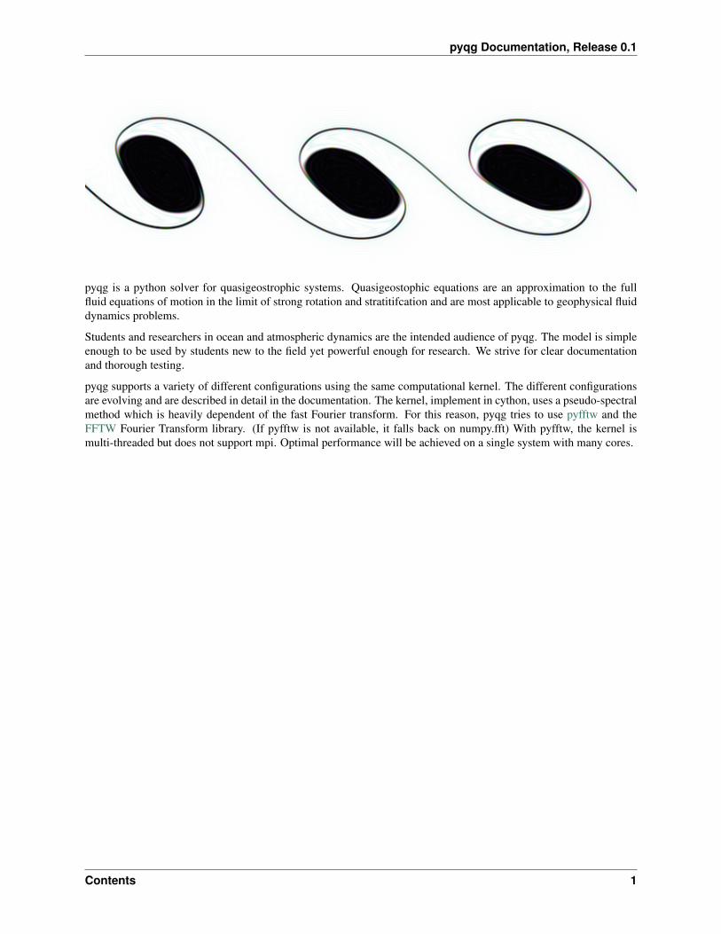
pyqg is a python solver for quasigeostrophic systems. Quasigeostophic equations are an approximation to the fullfluid equations of motion in the limit of strong rotation and stratitifcation and are most applicable to geophysical fluiddynamics problems.
Students and researchers in ocean and atmospheric dynamics are the intended audience of pyqg. The model is simpleenough to be used by students new to the field yet powerful enough for research. We strive for clear documentationand thorough testing.
pyqg supports a variety of different configurations using the same computational kernel. The different configurationsare evolving and are described in detail in the documentation. The kernel, implement in cython, uses a pseudo-spectralmethod which is heavily dependent of the fast Fourier transform. For this reason, pyqg tries to use pyfftw and theFFTW Fourier Transform library. (If pyfftw is not available, it falls back on numpy.fft) With pyfftw, the kernel ismulti-threaded but does not support mpi. Optimal performance will be achieved on a single system with many cores.
Contents 1

pyqg Documentation, Release 0.1
2 Contents
CHAPTER 1
Contents
1.1 Installation
1.1.1 Requirements
The only requirements are
• Python 2.7. (Python 3 support is in the works)
• numpy (1.6 or later)
• Cython (0.2 or later)
Because pyqg is a pseudo-spectral code, it realies heavily on fast-Fourier transforms (FFTs), which are the mainperformance bottlneck. For this reason, we try to use fftw (a fast, multithreaded, open source C library) and pyfftw(a python wrapper around fftw). These packages are optional, but they are strongly recommended for anyone doinghigh-resolution, numerically demanding simulations.
• fftw (3.3 or later)
• pyfftw (0.9.2 or later)
If pyqg can’t import pyfftw at compile time, it will fall back on numpy’s fft routines.
1.1.2 Instructions
In our opinion, the best way to get python and numpy is to use a distribution such as Anaconda (recommended)or Canopy. These provide robust package management and come with many other useful packages for scientificcomputing. The pyqg developers are mostly using anaconda.
Note: If you don’t want to use pyfftw and are content with numpy’s slower performance, you can skip ahead toInstalling pyqg.
3

pyqg Documentation, Release 0.1
Installing fftw and pyfftw can be slightly painful. Hopefully the instructions below are sufficient. If not, please sendfeedback.
Installing fftw and pyfftw
Once you have installed pyfftw via one of these paths, you can proceed to Installing pyqg.
The easy way: installing with conda
If you are using Anaconda, we have discovered that you can easily install pyffw using the conda command. Althoughpyfftw is not part of the main Anaconda distribution, it is distributed as a conda pacakge through several user channels.
There is a useful blog post describing how the pyfftw conda package was created. There are currently 13 pyfftw userpackages hosted on anaconda.org. Each has different dependencies and platform support (e.g. linux, windows, mac.)The nanshe channel version is the most popular and appears to have the broadest cross-platform support. We don’tknow who nanshe is, but we are greatful to him/her.
To install pyfftw from the conda-forge channel, open a terminal and run the command
$ conda install -c conda-forge pyfftw
The hard way: installing from source
This is the most difficult step for new users. You will probably have to build FFTW3 from source. However, if you areusing Ubuntu linux, you can save yourself some trouble by installing fftw using the apt package manager
$ sudo apt-get install libfftw3-dev libfftw3-doc
Otherwise you have to build FFTW3 from source. Your main resource for the FFTW homepage. Below we summarizethe steps
First download the source code.
$ wget http://www.fftw.org/fftw-3.3.4.tar.gz$ tar -xvzf fftw-3.3.4.tar.gz$ cd fftw-3.3.4
Then run the configure command
$ ./configure --enable-threads --enable-shared
Note: If you don’t have root privileges on your computer (e.g. on a shared cluster) the best approach is to ask yoursystem administrator to install FFTW3 for you. If that doesn’t work, you will have to install the FFTW3 libraries intoa location in your home directory (e.g. $HOME/fftw) and add the flag --prefix=$HOME/fftw to the configurecommand above.
Then build the software
$ make
Then install the software
4 Chapter 1. Contents

pyqg Documentation, Release 0.1
$ sudo make install
This will install the FFTW3 libraries into you system’s library directory. If you don’t have root privileges (see noteabove), remove the sudo. This will install the libraries into the prefix location you specified.
You are not done installing FFTW yet. pyfftw requires special versions of the FFTW library specialized to differentdata types (32-bit floats and double-long floars). You need to-configure and re-build FFTW two more times with extraflags.
$ ./configure --enable-threads --enable-shared --enable-float$ make$ sudo make install$ ./configure --enable-threads --enable-shared --enable-long-double$ make$ sudo make install
At this point, you FFTW installation is complete. We now move on to pyfftw. pyfftw is a python wrapper around theFFTW libraries. The easiest way to install it is using pip:
$ pip install pyfftw
or if you don’t have root privileges
$ pip install pyfftw --user
If this fails for some reason, you can manually download and install it according to the instructions on github. Firstclone the repository:
$ git clone https://github.com/hgomersall/pyFFTW.git
Then install it
$ cd pyFFTW$ python setup.py install
or
$ python setup.py install --user
if you don’t have root privileges. If you installed FFTW in a non-standard location (e.g. $HOME/fftw), you mighthave to do something tricky at this point to make sure pyfftw can find FFTW. (I figured this out once, but I can’tremember how.)
Installing pyqg
Note: The pyqg kernel is written in Cython and uses OpenMP to parallelise some operations for a performance boost.If you are using Mac OSX Yosemite or later OpenMP support is not available out of the box. While pyqg will stillrun without OpenMP, it will not be as fast as it can be. See Installing with OpenMP support on OSX below for moreinformation on installing on OSX with OpenMP support.
With pyfftw installed, you can now install pyqg. The easiest way is with pip:
$ pip install pyqg
1.1. Installation 5

pyqg Documentation, Release 0.1
You can also clone the pyqg git repository to use the latest development version.
$ git clone https://github.com/pyqg/pyqg.git
Then install pyqg on your system:
$ python setup.py install [--user]
(The --user flag is optional–use it if you don’t have root privileges.)
If you want to make changes in the code, set up the development mode:
$ python setup.py develop
pyqg is a work in progress, and we really encourage users to contribute to its Development
Installing with OpenMP support on OSX
There are two options for installing on OSX with OpenMP support. Both methods require using the Anaconda distri-bution of Python.
1. Using Homebrew
Install the GCC-5 compiler in /usr/local using Homebrew:
$ brew install gcc --without-multilib --with-fortran
Install Cython from the conda repository
$ conda install cython
Install pyqg using the homebrew gcc compiler
$ CC=/usr/local/bin/gcc-5 pip install pyqg
2. Using the HPC precompiled gcc binaries.
The HPC for Mac OSX sourceforge project has copies of the latest gcc precompiled for Mac OSX. Download thelatest version of gcc from the HPC site and follow the installation instructions.
Install Cython from the conda repository
$ conda install cython
Install pyqg using the HPC gcc compiler
$ CC=/usr/local/bin/gcc pip install pyqg
1.2 Equations Solved
A detailed description of the equations solved by the various pyqg models
6 Chapter 1. Contents
pyqg Documentation, Release 0.1
1.2.1 Equations For Two-Layer QG Model
The two-layer quasigeostrophic evolution equations are (1)
𝜕𝑡 𝑞1 + J (𝜓1 , 𝑞1) + 𝛽 𝜓1𝑥 = ssd ,
and (2)
𝜕𝑡 𝑞2 + J (𝜓2 , 𝑞2) + 𝛽 𝜓2𝑥 = −𝑟𝑒𝑘∇2𝜓2 + ssd ,
where the horizontal Jacobian is J (𝐴 ,𝐵) = 𝐴𝑥𝐵𝑦−𝐴𝑦𝐵𝑥. Also in (1) and (2) ssd denotes small-scale dissipation (inturbulence regimes, ssd absorbs enstrophy that cascates towards small scales). The linear bottom drag in (2) dissipateslarge-scale energy.
The potential vorticities are (3)
𝑞1 = ∇2𝜓1 + 𝐹1 (𝜓2 − 𝜓1) ,
and (4)
𝑞2 = ∇2𝜓2 + 𝐹2 (𝜓1 − 𝜓2) ,
where
𝐹1 ≡ 𝑘2𝑑1 + 𝛿2
, and 𝐹2 ≡ 𝛿 𝐹1 ,
with the deformation wavenumber
𝑘2𝑑 ≡ 𝑓20𝑔′𝐻1 +𝐻2
𝐻1𝐻2,
where 𝐻 = 𝐻1 +𝐻2 is the total depth at rest.
Forced-dissipative equations
We are interested in flows driven by baroclinic instabilty of a base-state shear 𝑈1 − 𝑈2. In this case the evolutionequations (1) and (2) become (5)
𝜕𝑡 𝑞1 + J (𝜓1 , 𝑞1) + 𝛽1 𝜓1𝑥 = ssd ,
and (6)
𝜕𝑡 𝑞2 + J (𝜓2 , 𝑞2) + 𝛽2 𝜓2𝑥 = −𝑟𝑒𝑘∇2𝜓2 + ssd ,
where the mean potential vorticity gradients are (9,10)
𝛽1 = 𝛽 + 𝐹1 (𝑈1 − 𝑈2) , and 𝛽2 = 𝛽 − 𝐹2 (𝑈1 − 𝑈2) .
Equations in Fourier space
We solve the two-layer QG system using a pseudo-spectral doubly-peridioc model. Fourier transforming the evolutionequations (5) and (6) gives (7)
𝜕𝑡 𝑞1 = −J (𝜓1 , 𝑞1) − i 𝑘 𝛽1 𝜓1 + ˆssd ,
1.2. Equations Solved 7

pyqg Documentation, Release 0.1
and
𝜕𝑡 𝑞2 = J (𝜓2 , 𝑞2) − 𝛽2 i 𝑘 𝜓2 + 𝑟𝑒𝑘 𝜅2 𝜓2 + ˆssd ,
where, in the pseudo-spectral spirit, J means the Fourier transform of the Jacobian i.e., we compute the products inphysical space, and then transform to Fourier space.
In Fourier space the “inversion relation” (3)-(4) is[−(𝜅2 + 𝐹1) 𝐹1
𝐹2 − (𝜅2 + 𝐹2)
]⏟ ⏞
≡M2
[𝜓1
𝜓2
]=
[𝑞1𝑞2
],
or equivalently [𝜓1
𝜓2
]=
1
det M2
[−(𝜅2 + 𝐹2) − 𝐹1
−𝐹2 − (𝜅2 + 𝐹1)
]⏟ ⏞
=M2−1
[𝑞1𝑞2
],
where
detM2 = 𝜅2(𝜅2 + 𝐹1 + 𝐹2
).
Marching forward
We use a third-order Adams-Bashford scheme
𝑞𝑛+1𝑖 = 𝐸𝑓 ×
[𝑞𝑛𝑖 +
∆𝑡
12
(23 ��𝑛
𝑖 − 16��𝑛−1𝑖 + 5��𝑛−2
𝑖
)],
where
��𝑛𝑖 ≡ −J (𝜓𝑛
𝑖 , 𝑞𝑛𝑖 ) − i 𝑘 𝛽𝑖 𝜓𝑛
𝑖 , 𝑖 = 1, 2 .
The AB3 is initialized with a first-order AB (or forward Euler)
𝑞1𝑖 = 𝐸𝑓 ×[𝑞0𝑖 + ∆𝑡��0
𝑖
],
The second step uses a second-order AB scheme
𝑞2𝑖 = 𝐸𝑓 ×[𝑞1𝑖 +
∆𝑡
2
(3 ��1
𝑖 − ��0𝑖
)].
The small-scale dissipation is achieve by a highly-selective exponential filter
𝐸𝑓 =
{e−23.6 (𝜅⋆−𝜅𝑐)
4
: 𝜅 ≥ 𝜅𝑐
1 : otherwise .
where the non-dimensional wavenumber is
𝜅⋆ ≡√
(𝑘∆𝑥)2 + (𝑙∆𝑦)2 ,
and 𝜅𝑐 is a (non-dimensional) wavenumber cutoff here taken as 65% of the Nyquist scale 𝜅⋆𝑛𝑦 = 𝜋. The parameter−23.6 is obtained from the requirement that the energy at the largest wanumber (𝜅⋆ = 𝜋) be zero whithin machinedouble precision:
log 10−15
(0.35𝜋)4≈ −23.5 .
For experiments with |𝑞𝑖| << 𝒪(1) one can use a smaller constant.
8 Chapter 1. Contents

pyqg Documentation, Release 0.1
Diagnostics
The kinetic energy is
𝐸 = 1𝐻 𝑆
∫12𝐻1 |∇𝜓1|2 + 1
2𝐻2 |∇𝜓2|2 𝑑𝑆 .
The potential enstrophy is
𝑍 = 1𝐻 𝑆
∫12𝐻1 𝑞
21 + 1
2𝐻2 𝑞22 𝑑𝑆 .
We can use the enstrophy to estimate the eddy turn-over timescale
𝑇𝑒 ≡2𝜋√𝑍.
1.2.2 Layered quasigeostrophic model
The N-layer quasigeostrophic (QG) potential vorticity is
𝑞1 = ∇2𝜓1 +𝑓20𝐻1
(𝜓2 − 𝜓1
𝑔′1
), 𝑛 = 1 ,
𝑞𝑛 = ∇2𝜓𝑛 +𝑓20𝐻𝑛
(𝜓𝑛−1 − 𝜓𝑛
𝑔′𝑛−1
− 𝜓𝑛 − 𝜓𝑛+1
𝑔′𝑛
), 𝑛 = 2,N − 1 ,
𝑞N = ∇2𝜓N +𝑓20𝐻N
(𝜓N−1 − 𝜓N
𝑔′N−1
)+
𝑓0𝐻N
ℎ𝑏(𝑥, 𝑦) , 𝑛 = N ,
where 𝑞𝑛 is the n’th layer QG potential vorticity, and 𝜓𝑛 is the streamfunction, 𝑓0 is the inertial frequency, n’th 𝐻𝑛
is the layer depth, and ℎ𝑏 is the bottom topography. (Note that in QG ℎ𝑏/𝐻N << 1.) Also the n’th buoyancy jump(reduced gravity) is
𝑔′𝑛 ≡ 𝑔𝜌𝑛 − 𝜌𝑛+1
𝜌𝑛,
where 𝑔 is the acceleration due to gravity and 𝜌𝑛 is the layer density.
The dynamics of the system is given by the evolution of PV. In particular, assuming a background flow with backgroundvelocity �� = (𝑈, 𝑉 ) such that
𝑢tot𝑛 = 𝑈𝑛 − 𝜓𝑛𝑦 ,
𝑣tot𝑛 = 𝑉𝑛 + 𝜓𝑛𝑥 ,
and
𝑞tot𝑛 = 𝑄𝑛 + 𝛿𝑛N
𝑓0𝐻N
ℎ𝑏 + 𝑞𝑛 ,
where 𝑄𝑛 + 𝛿𝑛N𝑓0𝐻N
ℎ𝑏 is n’th layer background PV, we obtain the evolution equations
𝑞𝑛𝑡 + J(𝜓𝑛, 𝑞𝑛 + 𝛿𝑛N𝑓0𝐻N
ℎ𝑏) + 𝑈𝑛(𝑞𝑛𝑥 + 𝛿𝑛N𝑓0𝐻N
ℎ𝑏𝑥) + 𝑉𝑛(𝑞𝑛𝑦 + 𝛿𝑛N𝑓0𝐻N
ℎ𝑏𝑦)+
𝑄𝑛𝑦𝜓𝑛𝑥 −𝑄𝑛𝑦𝜓𝑛𝑦 = ssd − 𝑟𝑒𝑘𝛿𝑛N∇2𝜓𝑛 , 𝑛 = 1,N ,
where ssd is stands for small scale dissipation, which is achieved by an spectral exponential filter or hyperviscosity,and 𝑟𝑒𝑘 is the linear bottom drag coefficient. The Dirac delta, 𝛿𝑛𝑁 , indicates that the drag is only applied in the bottomlayer.
1.2. Equations Solved 9

pyqg Documentation, Release 0.1
Equations in spectral space
The evolutionary equation in spectral space is
𝑞𝑛𝑡 + (i𝑘𝑈 + i𝑙𝑉 )
(𝑞𝑛 + 𝛿𝑛N
𝑓0𝐻N
ℎ𝑏
)+ (i𝑘 𝑄𝑦 −−i𝑙 𝑄𝑥)𝜓𝑛 + J(𝜓𝑛, 𝑞𝑛 + 𝛿𝑛N
𝑓0𝐻N
ℎ𝑏)
= ssd + i𝛿𝑛N𝑟𝑒𝑘𝜅2𝜓𝑛 , 𝑖 = 1,N ,
where 𝜅2 = 𝑘2 + 𝑙2. Also, in the pseudo-spectral spirit we write the transform of the nonlinear terms and the non-constant coefficient linear term as the transform of the products, calculated in physical space, as opposed to doubleconvolution sums. That is J is the Fourier transform of Jacobian computed in physical space.
The inversion relationship is
𝑞𝑖 =(S− 𝜅2I
)𝜓𝑖 ,
where I is the N × N identity matrix, and the stretching matrix is
S ≡ 𝑓20
⎡⎢⎢⎢⎢⎢⎢⎢⎢⎢⎢⎢⎢⎣
− 1𝑔′1𝐻1
1𝑔′1𝐻1
0 . . .
0...
. . . . . . . . .1
𝑔′𝑖−1𝐻𝑖
−(
1𝑔′𝑖−1𝐻𝑖
+ 1𝑔′𝑖𝐻𝑖
)1
𝑔′𝑖𝐻𝑖
. . . . . . . . .
. . . 0 1𝑔′N−1𝐻N
− 1𝑔′N−1𝐻N
⎤⎥⎥⎥⎥⎥⎥⎥⎥⎥⎥⎥⎥⎦.
Energy spectrum
The equation for the energy spectrum,
𝐸(𝑘, 𝑙) ≡ 1
2𝐻
N∑𝑖=1
𝐻𝑖𝜅2|𝜓𝑖|2 +
1
2𝐻
N−1∑𝑖=1
𝑓20𝑔′𝑖
|𝜓𝑖 − 𝜓𝑖+1|2 ,
is
𝑑
𝑑𝑡𝐸(𝑘, 𝑙) =
1
𝐻
N∑𝑖=1
𝐻𝑖Re[𝜓⋆𝑖 J(𝜓𝑖,∇2𝜓𝑖)] +
1
𝐻
N∑𝑖=1
𝐻𝑖Re[𝜓⋆𝑖
ˆJ(𝜓𝑖, (S𝜓)𝑖)]
+1
𝐻
N∑𝑖=1
𝐻𝑖(𝑘𝑈𝑖 + 𝑙𝑉𝑖) Re[𝑖 𝜓⋆𝑖 (S𝜓𝑖)] −𝑟𝑒𝑘
𝐻N
𝐻𝜅2|𝜓N|2 + 𝐸ssd ,
where ⋆ stands for complex conjugation, and the terms above on the right represent, from left to right,
I: The spectral divergence of the kinetic energy flux;
II: The spectral divergence of the potential energy flux;
III: The spectrum of the potential energy generation;
IV: The spectrum of the energy dissipation by linear bottom drag;
V: The spectrum of energy loss due to small scale dissipation.
We assume that 𝑉 is relatively small, and that, in statistical steady state, the budget above is dominated by I throughIV.
10 Chapter 1. Contents

pyqg Documentation, Release 0.1
Enstrophy spectrum
Similarly the evolution of the barotropic enstrophy spectrum,
𝑍(𝑘, 𝑙) ≡ 1
2𝐻
N∑𝑖=1
𝐻𝑖|𝑞𝑖|2 ,
is governed by
𝑑
𝑑𝑡𝑍(𝑘, 𝑙) = Re[𝑞⋆𝑖 J(𝜓𝑖, 𝑞𝑖)]−(𝑘𝑄𝑦 − 𝑙𝑄𝑥)Re[(S𝜓⋆
𝑖 )𝜓𝑖] + 𝑍ssd ,
where the terms above on the right represent, from left to right,
I: The spectral divergence of barotropic potential enstrophy flux;
II: The spectrum of barotropic potential enstrophy generation;
III: The spectrum of barotropic potential enstrophy loss due to small scale dissipation.
The enstrophy dissipation is concentrated at the smallest scales resolved in the model and, in statistical steady state,we expect the budget above to be dominated by the balance between I and II.
1.2.3 Special case: two-layer model
With N = 2, an alternative notation for the perturbation of potential vorticities can be written as
𝑞1 = ∇2𝜓1 + 𝐹1(𝜓2 − 𝜓1)
𝑞2 = ∇2𝜓2 + 𝐹2(𝜓1 − 𝜓2) ,
where we use the following definitions where
𝐹1 ≡ 𝑘2𝑑1 + 𝛿2
, and 𝐹2 ≡ 𝛿 𝐹1 ,
with the deformation wavenumber
𝑘2𝑑 ≡ 𝑓20𝑔
𝐻1 +𝐻2
𝐻1𝐻2.
With this notation, the “stretching matrix” is simply
S =
[−𝐹1 𝐹1
𝐹2 − +𝐹2
].
The inversion relationship in Fourier space is[𝜓1
𝜓2
]=
1
det B
[−(𝜅2 + 𝐹2) − 𝐹1
−𝐹2 − (𝜅2 + 𝐹1)
] [𝑞1𝑞2
],
where
detB = 𝜅2(𝜅2 + 𝐹1 + 𝐹2
).
1.2. Equations Solved 11
pyqg Documentation, Release 0.1
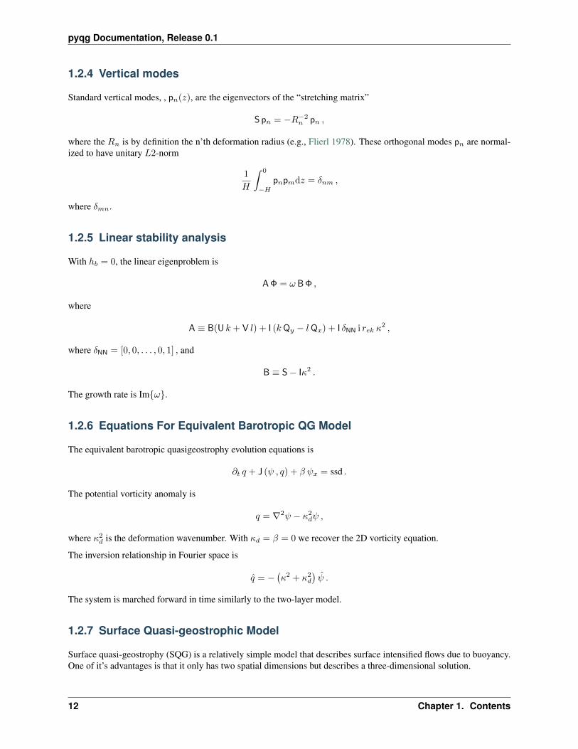
1.2.4 Vertical modes
Standard vertical modes, , p𝑛(𝑧), are the eigenvectors of the “stretching matrix”
S p𝑛 = −𝑅−2𝑛 p𝑛 ,
where the 𝑅𝑛 is by definition the n’th deformation radius (e.g., Flierl 1978). These orthogonal modes p𝑛 are normal-ized to have unitary 𝐿2-norm
1
𝐻
∫ 0
−𝐻
p𝑛p𝑚d𝑧 = 𝛿𝑛𝑚 ,
where 𝛿𝑚𝑛.
1.2.5 Linear stability analysis
With ℎ𝑏 = 0, the linear eigenproblem is
AΦ = 𝜔 BΦ ,
where
A ≡ B(U 𝑘 + V 𝑙) + I (𝑘Q𝑦 − 𝑙Q𝑥) + I 𝛿NN i 𝑟𝑒𝑘 𝜅2 ,
where 𝛿NN = [0, 0, . . . , 0, 1] , and
B ≡ S− I𝜅2 .
The growth rate is Im{𝜔}.
1.2.6 Equations For Equivalent Barotropic QG Model
The equivalent barotropic quasigeostrophy evolution equations is
𝜕𝑡 𝑞 + J (𝜓 , 𝑞) + 𝛽 𝜓𝑥 = ssd .
The potential vorticity anomaly is
𝑞 = ∇2𝜓 − 𝜅2𝑑𝜓 ,
where 𝜅2𝑑 is the deformation wavenumber. With 𝜅𝑑 = 𝛽 = 0 we recover the 2D vorticity equation.
The inversion relationship in Fourier space is
𝑞 = −(𝜅2 + 𝜅2𝑑
)𝜓 .
The system is marched forward in time similarly to the two-layer model.
1.2.7 Surface Quasi-geostrophic Model
Surface quasi-geostrophy (SQG) is a relatively simple model that describes surface intensified flows due to buoyancy.One of it’s advantages is that it only has two spatial dimensions but describes a three-dimensional solution.
12 Chapter 1. Contents

pyqg Documentation, Release 0.1
The evolution equation is
𝜕𝑡𝑏+ 𝐽(𝜓, 𝑏) = 0 , at 𝑧 = 0 ,
where 𝑏 = 𝜓𝑧 is the buoyancy.
The interior potential vorticity is zero. Hence
𝜕
𝜕𝑧
(𝑓20𝑁2
𝜕𝜓
𝜕𝑧
)+ ∇2𝜓 = 0 ,
where 𝑁 is the buoyancy frequency and 𝑓0 is the Coriolis parameter. In the SQG model both 𝑁 and 𝑓0 are constants.The boundary conditions for this elliptic problem in a semi-infinite vertical domain are
𝑏 = 𝜓𝑧 , and 𝑧 = 0 ,
and
𝜓 = 0, at 𝑧 → −∞ ,
The solutions to the elliptic problem above, in horizontal Fourier space, gives the inversion relationship betweensurface buoyancy and surface streamfunction
𝜓 =𝑓0𝑁
1
𝜅�� , at 𝑧 = 0 ,
The SQG evolution equation is marched forward similarly to the two-layer model.
1.3 Examples
1.3.1 Two Layer QG Model Example
Here is a quick overview of how to use the two-layer model. See the :py:class:pyqg.QGModel api documentationfor further details.
First import numpy, matplotlib, and pyqg:
import numpy as npfrom matplotlib import pyplot as plt%matplotlib inlineimport pyqg
Vendor: Continuum Analytics, Inc.Package: mklMessage: trial mode expires in 19 daysVendor: Continuum Analytics, Inc.Package: mklMessage: trial mode expires in 19 daysVendor: Continuum Analytics, Inc.Package: mklMessage: trial mode expires in 19 days
Initialize and Run the Model
Here we set up a model which will run for 10 years and start averaging after 5 years. There are lots of parameters thatcan be specified as keyword arguments but we are just using the defaults.
1.3. Examples 13

pyqg Documentation, Release 0.1
year = 24*60*60*360.m = pyqg.QGModel(tmax=10*year, twrite=10000, tavestart=5*year)m.run()
t= 72000000, tc= 10000: cfl=0.105787, ke=0.000565075t= 144000000, tc= 20000: cfl=0.092474, ke=0.000471924t= 216000000, tc= 30000: cfl=0.104418, ke=0.000525463t= 288000000, tc= 40000: cfl=0.089834, ke=0.000502072
Visualize Output
We access the actual pv values through the attribute m.q. The first axis of q corresponds with the layer number.(Remeber that in python, numbering starts at 0.)
q_upper = m.q[0] + m.Qy[0]*m.yplt.contourf(m.x, m.y, q_upper, 12, cmap='RdBu_r')plt.xlabel('x'); plt.ylabel('y'); plt.title('Upper Layer PV')plt.colorbar();
Plot Diagnostics
The model automatically accumulates averages of certain diagnostics. We can find out what diagnostics are availableby calling
m.describe_diagnostics()
14 Chapter 1. Contents

pyqg Documentation, Release 0.1
NAME | DESCRIPTION--------------------------------------------------------------------------------APEflux | spectral flux of available potential energyAPEgen | total APE generationAPEgenspec | spectrum of APE generationEKE | mean eddy kinetic energyEKEdiss | total energy dissipation by bottom dragEnsspec | enstrophy spectrumKEflux | spectral flux of kinetic energyKEspec | kinetic energy spectrumentspec | barotropic enstrophy spectrumq | QGPV
To look at the wavenumber energy spectrum, we plot the KEspec diagnostic. (Note that summing along the l-axis, asin this example, does not give us a true isotropic wavenumber spectrum.)
kespec_u = m.get_diagnostic('KEspec')[0].sum(axis=0)kespec_l = m.get_diagnostic('KEspec')[1].sum(axis=0)plt.loglog( m.kk, kespec_u, '.-' )plt.loglog( m.kk, kespec_l, '.-' )plt.legend(['upper layer','lower layer'], loc='lower left')plt.ylim([1e-9,1e-3]); plt.xlim([m.kk.min(), m.kk.max()])plt.xlabel(r'k (m$^{-1}$)'); plt.grid()plt.title('Kinetic Energy Spectrum');
We can also plot the spectral fluxes of energy.
ebud = [ m.get_diagnostic('APEgenspec').sum(axis=0),m.get_diagnostic('APEflux').sum(axis=0),
1.3. Examples 15

pyqg Documentation, Release 0.1
m.get_diagnostic('KEflux').sum(axis=0),-m.rek*m.del2*m.get_diagnostic('KEspec')[1].sum(axis=0)*m.M**2 ]
ebud.append(-np.vstack(ebud).sum(axis=0))ebud_labels = ['APE gen','APE flux','KE flux','Diss.','Resid.'][plt.semilogx(m.kk, term) for term in ebud]plt.legend(ebud_labels, loc='upper right')plt.xlim([m.kk.min(), m.kk.max()])plt.xlabel(r'k (m$^{-1}$)'); plt.grid()plt.title('Spectral Energy Transfers');
1.3.2 Fully developed baroclinic instability of a 3-layer flow
import numpy as npfrom numpy import pifrom matplotlib import pyplot as plt%matplotlib inline
import pyqgfrom pyqg import diagnostic_tools as tools
Vendor: Continuum Analytics, Inc.Package: mklMessage: trial mode expires in 21 daysVendor: Continuum Analytics, Inc.Package: mklMessage: trial mode expires in 21 daysVendor: Continuum Analytics, Inc.
16 Chapter 1. Contents
pyqg Documentation, Release 0.1
Package: mklMessage: trial mode expires in 21 days
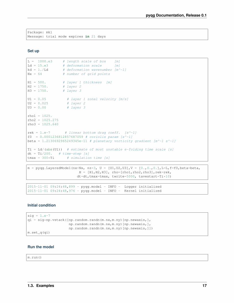
Set up
L = 1000.e3 # length scale of box [m]Ld = 15.e3 # deformation scale [m]kd = 1./Ld # deformation wavenumber [m^-1]Nx = 64 # number of grid points
H1 = 500. # layer 1 thickness [m]H2 = 1750. # layer 2H3 = 1750. # layer 3
U1 = 0.05 # layer 1 zonal velocity [m/s]U2 = 0.025 # layer 2U3 = 0.00 # layer 3
rho1 = 1025.rho2 = 1025.275rho3 = 1025.640
rek = 1.e-7 # linear bottom drag coeff. [s^-1]f0 = 0.0001236812857687059 # coriolis param [s^-1]beta = 1.2130692965249345e-11 # planetary vorticity gradient [m^-1 s^-1]
Ti = Ld/(abs(U1)) # estimate of most unstable e-folding time scale [s]dt = Ti/200. # time-step [s]tmax = 300*Ti # simulation time [s]
m = pyqg.LayeredModel(nx=Nx, nz=3, U = [U1,U2,U3],V = [0.,0.,0.],L=L,f=f0,beta=beta,H = [H1,H2,H3], rho=[rho1,rho2,rho3],rek=rek,dt=dt,tmax=tmax, twrite=5000, tavestart=Ti*10)
2015-11-01 09:24:48,899 - pyqg.model - INFO - Logger initialized2015-11-01 09:24:48,976 - pyqg.model - INFO - Kernel initialized
Initial condition
sig = 1.e-7qi = sig*np.vstack([np.random.randn(m.nx,m.ny)[np.newaxis,],
np.random.randn(m.nx,m.ny)[np.newaxis,],np.random.randn(m.nx,m.ny)[np.newaxis,]])
m.set_q(qi)
Run the model
m.run()
1.3. Examples 17
pyqg Documentation, Release 0.1
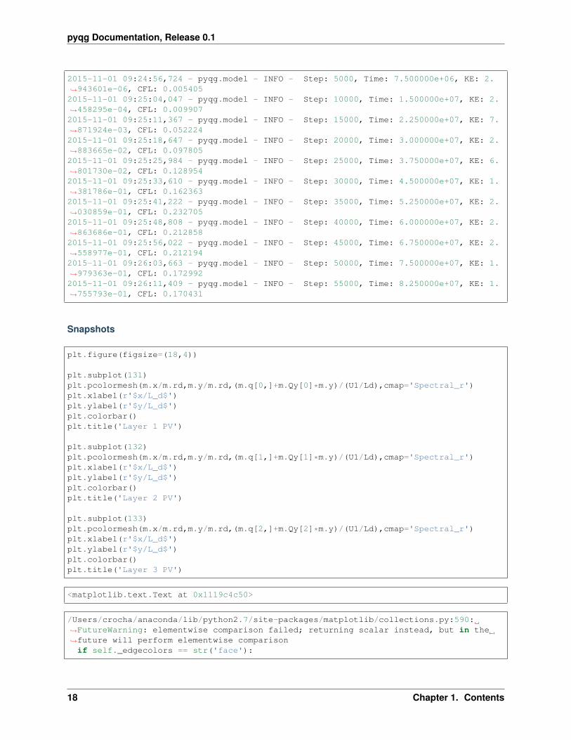
2015-11-01 09:24:56,724 - pyqg.model - INFO - Step: 5000, Time: 7.500000e+06, KE: 2.→˓943601e-06, CFL: 0.0054052015-11-01 09:25:04,047 - pyqg.model - INFO - Step: 10000, Time: 1.500000e+07, KE: 2.→˓458295e-04, CFL: 0.0099072015-11-01 09:25:11,367 - pyqg.model - INFO - Step: 15000, Time: 2.250000e+07, KE: 7.→˓871924e-03, CFL: 0.0522242015-11-01 09:25:18,647 - pyqg.model - INFO - Step: 20000, Time: 3.000000e+07, KE: 2.→˓883665e-02, CFL: 0.0978052015-11-01 09:25:25,984 - pyqg.model - INFO - Step: 25000, Time: 3.750000e+07, KE: 6.→˓801730e-02, CFL: 0.1289542015-11-01 09:25:33,610 - pyqg.model - INFO - Step: 30000, Time: 4.500000e+07, KE: 1.→˓381786e-01, CFL: 0.1623632015-11-01 09:25:41,222 - pyqg.model - INFO - Step: 35000, Time: 5.250000e+07, KE: 2.→˓030859e-01, CFL: 0.2327052015-11-01 09:25:48,808 - pyqg.model - INFO - Step: 40000, Time: 6.000000e+07, KE: 2.→˓863686e-01, CFL: 0.2128582015-11-01 09:25:56,022 - pyqg.model - INFO - Step: 45000, Time: 6.750000e+07, KE: 2.→˓558977e-01, CFL: 0.2121942015-11-01 09:26:03,663 - pyqg.model - INFO - Step: 50000, Time: 7.500000e+07, KE: 1.→˓979363e-01, CFL: 0.1729922015-11-01 09:26:11,409 - pyqg.model - INFO - Step: 55000, Time: 8.250000e+07, KE: 1.→˓755793e-01, CFL: 0.170431
Snapshots
plt.figure(figsize=(18,4))
plt.subplot(131)plt.pcolormesh(m.x/m.rd,m.y/m.rd,(m.q[0,]+m.Qy[0]*m.y)/(U1/Ld),cmap='Spectral_r')plt.xlabel(r'$x/L_d$')plt.ylabel(r'$y/L_d$')plt.colorbar()plt.title('Layer 1 PV')
plt.subplot(132)plt.pcolormesh(m.x/m.rd,m.y/m.rd,(m.q[1,]+m.Qy[1]*m.y)/(U1/Ld),cmap='Spectral_r')plt.xlabel(r'$x/L_d$')plt.ylabel(r'$y/L_d$')plt.colorbar()plt.title('Layer 2 PV')
plt.subplot(133)plt.pcolormesh(m.x/m.rd,m.y/m.rd,(m.q[2,]+m.Qy[2]*m.y)/(U1/Ld),cmap='Spectral_r')plt.xlabel(r'$x/L_d$')plt.ylabel(r'$y/L_d$')plt.colorbar()plt.title('Layer 3 PV')
<matplotlib.text.Text at 0x1119c4c50>
/Users/crocha/anaconda/lib/python2.7/site-packages/matplotlib/collections.py:590:→˓FutureWarning: elementwise comparison failed; returning scalar instead, but in the→˓future will perform elementwise comparisonif self._edgecolors == str('face'):
18 Chapter 1. Contents

pyqg Documentation, Release 0.1
pyqg has a built-in method that computes the vertical modes.
print "The first baroclinic deformation radius is", m.radii[1]/1.e3, "km"print "The second baroclinic deformation radius is", m.radii[2]/1.e3, "km"
The first baroclinic deformation radius is 15.375382786 kmThe second baroclinic deformation radius is 7.975516272 km
We can project the solution onto the modes
pn = m.modal_projection(m.p)
plt.figure(figsize=(18,4))
plt.subplot(131)plt.pcolormesh(m.x/m.rd,m.y/m.rd,pn[0]/(U1*Ld),cmap='Spectral_r')plt.xlabel(r'$x/L_d$')plt.ylabel(r'$y/L_d$')plt.colorbar()plt.title('Barotropic streamfunction')
plt.subplot(132)plt.pcolormesh(m.x/m.rd,m.y/m.rd,pn[1]/(U1*Ld),cmap='Spectral_r')plt.xlabel(r'$x/L_d$')plt.ylabel(r'$y/L_d$')plt.colorbar()plt.title('1st baroclinic streamfunction')
plt.subplot(133)plt.pcolormesh(m.x/m.rd,m.y/m.rd,pn[2]/(U1*Ld),cmap='Spectral_r')plt.xlabel(r'$x/L_d$')plt.ylabel(r'$y/L_d$')plt.colorbar()plt.title('2nd baroclinic streamfunction')
<matplotlib.text.Text at 0x11273f350>
1.3. Examples 19

pyqg Documentation, Release 0.1
Diagnostics
kr, kespec_1 = tools.calc_ispec(m,m.get_diagnostic('KEspec')[0])_, kespec_2 = tools.calc_ispec(m,m.get_diagnostic('KEspec')[1])_, kespec_3 = tools.calc_ispec(m,m.get_diagnostic('KEspec')[2])
plt.loglog( kr, kespec_1, '.-' )plt.loglog( kr, kespec_2, '.-' )plt.loglog( kr, kespec_3, '.-' )
plt.legend(['layer 1','layer 2', 'layer 3'], loc='lower left')plt.ylim([1e-14,1e-6]); plt.xlim([m.kk.min(), m.kk.max()])plt.xlabel(r'k (m$^{-1}$)'); plt.grid()plt.title('Kinetic Energy Spectrum');
By default the modal KE and PE spectra are also calculated
20 Chapter 1. Contents

pyqg Documentation, Release 0.1
kr, modal_kespec_1 = tools.calc_ispec(m,m.get_diagnostic('KEspec_modal')[0])_, modal_kespec_2 = tools.calc_ispec(m,m.get_diagnostic('KEspec_modal')[1])_, modal_kespec_3 = tools.calc_ispec(m,m.get_diagnostic('KEspec_modal')[2])
_, modal_pespec_2 = tools.calc_ispec(m,m.get_diagnostic('PEspec_modal')[0])_, modal_pespec_3 = tools.calc_ispec(m,m.get_diagnostic('PEspec_modal')[1])
plt.figure(figsize=(15,5))
plt.subplot(121)plt.loglog( kr, modal_kespec_1, '.-' )plt.loglog( kr, modal_kespec_2, '.-' )plt.loglog( kr, modal_kespec_3, '.-' )
plt.legend(['barotropic ','1st baroclinic', '2nd baroclinic'], loc='lower left')plt.ylim([1e-14,1e-6]); plt.xlim([m.kk.min(), m.kk.max()])plt.xlabel(r'k (m$^{-1}$)'); plt.grid()plt.title('Kinetic Energy Spectra');
plt.subplot(122)plt.loglog( kr, modal_pespec_2, '.-' )plt.loglog( kr, modal_pespec_3, '.-' )
plt.legend(['1st baroclinic', '2nd baroclinic'], loc='lower left')plt.ylim([1e-14,1e-6]); plt.xlim([m.kk.min(), m.kk.max()])plt.xlabel(r'k (m$^{-1}$)'); plt.grid()plt.title('Potential Energy Spectra');
_, APEgenspec = tools.calc_ispec(m,m.get_diagnostic('APEgenspec'))_, APEflux = tools.calc_ispec(m,m.get_diagnostic('APEflux'))_, KEflux = tools.calc_ispec(m,m.get_diagnostic('KEflux'))_, KEspec = tools.calc_ispec(m,m.get_diagnostic('KEspec')[1]*m.M**2)
ebud = [ APEgenspec,APEflux,KEflux,-m.rek*(m.Hi[-1]/m.H)*KEspec ]
ebud.append(-np.vstack(ebud).sum(axis=0))
1.3. Examples 21

pyqg Documentation, Release 0.1
ebud_labels = ['APE gen','APE flux div.','KE flux div.','Diss.','Resid.'][plt.semilogx(kr, term) for term in ebud]plt.legend(ebud_labels, loc='upper right')plt.xlim([m.kk.min(), m.kk.max()])plt.xlabel(r'k (m$^{-1}$)'); plt.grid()plt.title('Spectral Energy Transfers');
The dynamics here is similar to the reference experiment of Larichev & Held (1995). The APE generated throughbaroclinic instability is fluxed towards deformation length scales, where it is converted into KE. The KE the experi-ments and inverse tranfer, cascading up to the scale of the domain. The mechanical bottom drag essentially removesthe large scale KE.
1.3.3 Barotropic Model
Here will will use pyqg to reproduce the results of the paper: J. C. Mcwilliams (1984). The emergence of isolatedcoherent vortices in turbulent flow. Journal of Fluid Mechanics, 146, pp 21-43 doi:10.1017/S0022112084001750
import numpy as npimport matplotlib.pyplot as plt%matplotlib inlineimport pyqg
McWilliams performed freely-evolving 2D turbulence (𝑅𝑑 = ∞, 𝛽 = 0) experiments on a 2𝜋 × 2𝜋 periodic box.
# create the model objectm = pyqg.BTModel(L=2.*np.pi, nx=256,
beta=0., H=1., rek=0., rd=None,tmax=40, dt=0.001, taveint=1,
22 Chapter 1. Contents
pyqg Documentation, Release 0.1
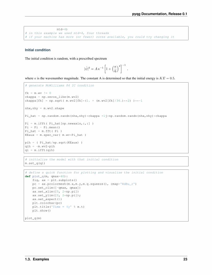
ntd=4)# in this example we used ntd=4, four threads# if your machine has more (or fewer) cores available, you could try changing it
Initial condition
The initial condition is random, with a prescribed spectrum
|𝜓|2 = 𝐴𝜅−1
[1 +
(𝜅6
)4]−1
,
where 𝜅 is the wavenumber magnitude. The constant A is determined so that the initial energy is 𝐾𝐸 = 0.5.
# generate McWilliams 84 IC condition
fk = m.wv != 0ckappa = np.zeros_like(m.wv2)ckappa[fk] = np.sqrt( m.wv2[fk]*(1. + (m.wv2[fk]/36.)**2) )**-1
nhx,nhy = m.wv2.shape
Pi_hat = np.random.randn(nhx,nhy)*ckappa +1j*np.random.randn(nhx,nhy)*ckappa
Pi = m.ifft( Pi_hat[np.newaxis,:,:] )Pi = Pi - Pi.mean()Pi_hat = m.fft( Pi )KEaux = m.spec_var( m.wv*Pi_hat )
pih = ( Pi_hat/np.sqrt(KEaux) )qih = -m.wv2*pihqi = m.ifft(qih)
# initialize the model with that initial conditionm.set_q(qi)
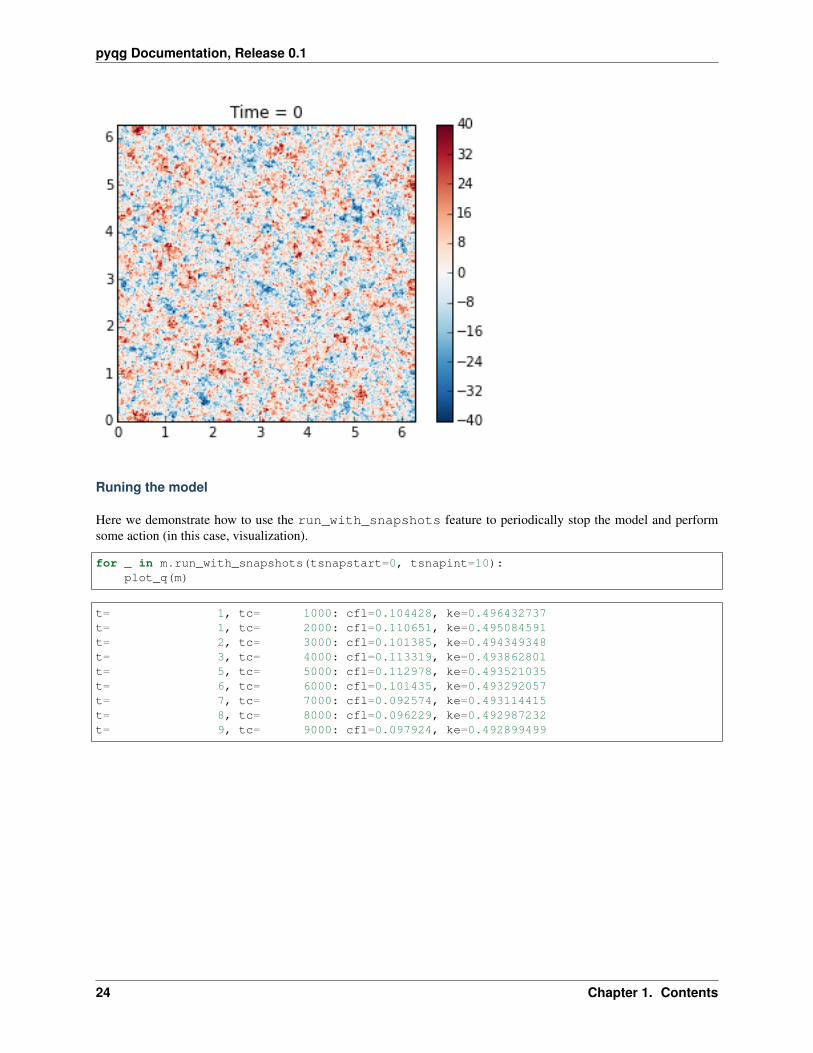
# define a quick function for plotting and visualize the initial conditiondef plot_q(m, qmax=40):
fig, ax = plt.subplots()pc = ax.pcolormesh(m.x,m.y,m.q.squeeze(), cmap='RdBu_r')pc.set_clim([-qmax, qmax])ax.set_xlim([0, 2*np.pi])ax.set_ylim([0, 2*np.pi]);ax.set_aspect(1)plt.colorbar(pc)plt.title('Time = %g' % m.t)plt.show()
plot_q(m)
1.3. Examples 23
pyqg Documentation, Release 0.1
Runing the model
Here we demonstrate how to use the run_with_snapshots feature to periodically stop the model and performsome action (in this case, visualization).
for _ in m.run_with_snapshots(tsnapstart=0, tsnapint=10):plot_q(m)
t= 1, tc= 1000: cfl=0.104428, ke=0.496432737t= 1, tc= 2000: cfl=0.110651, ke=0.495084591t= 2, tc= 3000: cfl=0.101385, ke=0.494349348t= 3, tc= 4000: cfl=0.113319, ke=0.493862801t= 5, tc= 5000: cfl=0.112978, ke=0.493521035t= 6, tc= 6000: cfl=0.101435, ke=0.493292057t= 7, tc= 7000: cfl=0.092574, ke=0.493114415t= 8, tc= 8000: cfl=0.096229, ke=0.492987232t= 9, tc= 9000: cfl=0.097924, ke=0.492899499
24 Chapter 1. Contents

pyqg Documentation, Release 0.1
t= 9, tc= 10000: cfl=0.103278, ke=0.492830631t= 10, tc= 11000: cfl=0.102686, ke=0.492775849t= 11, tc= 12000: cfl=0.099865, ke=0.492726644t= 12, tc= 13000: cfl=0.110933, ke=0.492679673t= 13, tc= 14000: cfl=0.102899, ke=0.492648562t= 14, tc= 15000: cfl=0.102052, ke=0.492622263t= 15, tc= 16000: cfl=0.106399, ke=0.492595449t= 16, tc= 17000: cfl=0.122508, ke=0.492569708t= 17, tc= 18000: cfl=0.120618, ke=0.492507272t= 19, tc= 19000: cfl=0.103734, ke=0.492474633
1.3. Examples 25

pyqg Documentation, Release 0.1
t= 20, tc= 20000: cfl=0.113210, ke=0.492452605t= 21, tc= 21000: cfl=0.095246, ke=0.492439588t= 22, tc= 22000: cfl=0.092449, ke=0.492429553t= 23, tc= 23000: cfl=0.115412, ke=0.492419773t= 24, tc= 24000: cfl=0.125958, ke=0.492407434t= 25, tc= 25000: cfl=0.098588, ke=0.492396021t= 26, tc= 26000: cfl=0.103689, ke=0.492387002t= 27, tc= 27000: cfl=0.103893, ke=0.492379606t= 28, tc= 28000: cfl=0.108417, ke=0.492371082t= 29, tc= 29000: cfl=0.112969, ke=0.492361675
26 Chapter 1. Contents

pyqg Documentation, Release 0.1
t= 30, tc= 30000: cfl=0.127132, ke=0.492352666t= 31, tc= 31000: cfl=0.122900, ke=0.492331664t= 32, tc= 32000: cfl=0.110486, ke=0.492317502t= 33, tc= 33000: cfl=0.101901, ke=0.492302225t= 34, tc= 34000: cfl=0.099996, ke=0.492294952t= 35, tc= 35000: cfl=0.106513, ke=0.492290743t= 36, tc= 36000: cfl=0.121426, ke=0.492286228t= 37, tc= 37000: cfl=0.125573, ke=0.492283246t= 38, tc= 38000: cfl=0.108975, ke=0.492280378t= 38, tc= 39000: cfl=0.110105, ke=0.492278000
1.3. Examples 27

pyqg Documentation, Release 0.1
t= 39, tc= 40000: cfl=0.104794, ke=0.492275760
The genius of McWilliams (1984) was that he showed that the initial random vorticity field organizes itself into strongcoherent vortices. This is true in significant part of the parameter space. This was previously suspected but unproven,mainly because people did not have computer resources to run the simulation long enough. Thirty years later we canperform such simulations in a couple of minutes on a laptop!
Also, note that the energy is nearly conserved, as it should be, and this is a nice test of the model.
Plotting spectra
energy = m.get_diagnostic('KEspec')enstrophy = m.get_diagnostic('Ensspec')
# this makes it easy to calculate an isotropic spectrumfrom pyqg import diagnostic_tools as toolskr, energy_iso = tools.calc_ispec(m,energy.squeeze())_, enstrophy_iso = tools.calc_ispec(m,enstrophy.squeeze())
ks = np.array([3.,80])es = 5*ks**-4plt.loglog(kr,energy_iso)plt.loglog(ks,es,'k--')plt.text(2.5,.0001,r'$k^{-4}$',fontsize=20)plt.ylim(1.e-10,1.e0)plt.xlabel('wavenumber')plt.title('Energy Spectrum')
<matplotlib.text.Text at 0x10c1b1a90>
28 Chapter 1. Contents

pyqg Documentation, Release 0.1
ks = np.array([3.,80])es = 5*ks**(-5./3)plt.loglog(kr,enstrophy_iso)plt.loglog(ks,es,'k--')plt.text(5.5,.01,r'$k^{-5/3}$',fontsize=20)plt.ylim(1.e-3,1.e0)plt.xlabel('wavenumber')plt.title('Enstrophy Spectrum')
<matplotlib.text.Text at 0x10b5d2f50>
1.3. Examples 29

pyqg Documentation, Release 0.1
1.3.4 Surface Quasi-Geostrophic (SQG) Model
Here will will use pyqg to reproduce the results of the paper: I. M. Held, R. T. Pierrehumbert, S. T. Garner andK. L. Swanson (1985). Surface quasi-geostrophic dynamics. Journal of Fluid Mechanics, 282, pp 1-20 [doi:: http://dx.doi.org/10.1017/S0022112095000012)
import matplotlib.pyplot as pltimport numpy as npfrom numpy import pi%matplotlib inlinefrom pyqg import sqg_model
Vendor: Continuum Analytics, Inc.Package: mklMessage: trial mode expires in 21 daysVendor: Continuum Analytics, Inc.Package: mklMessage: trial mode expires in 21 daysVendor: Continuum Analytics, Inc.Package: mklMessage: trial mode expires in 21 days
Surface quasi-geostrophy (SQG) is a relatively simple model that describes surface intensified flows due to buoyancy.One of it’s advantages is that it only has two spatial dimensions but describes a three-dimensional solution.
If we define 𝑏 to be the buoyancy, then the evolution equation for buoyancy at each the top and bottom surface is
𝜕𝑡𝑏+ 𝐽(𝜓, 𝑏) = 0.
30 Chapter 1. Contents

pyqg Documentation, Release 0.1
The invertibility relation between the streamfunction, 𝜓, and the buoyancy, 𝑏, is hydrostatic balance
𝑏 = 𝜕𝑧𝜓.
Using the fact that the Potential Vorticity is exactly zero in the interior of the domain and that the domain is semi-infinite, yields that the inversion in Fourier space is,
�� = 𝐾𝜓.
Held et al. studied several different cases, the first of which was the nonlinear evolution of an elliptical vortex. Thereare several other cases that they studied and people are welcome to adapt the code to study those as well. But here wefocus on this first example for pedagogical reasons.
# create the model objectyear = 1.m = sqg_model.SQGModel(L=2.*pi,nx=512, tmax = 26.005,
beta = 0., Nb = 1., H = 1., rek = 0., rd = None, dt = 0.005,taveint=1, twrite=400, ntd=4)
# in this example we used ntd=4, four threads# if your machine has more (or fewer) cores available, you could try changing it
INFO: Logger initializedINFO: Kernel initialized
Initial condition
The initial condition is an elliptical vortex,
𝑏 = 0.01 exp(−(𝑥2 + (4𝑦)2)/(𝐿/𝑦)2
where 𝐿 is the length scale of the vortex in the 𝑥 direction. The amplitude is 0.01, which sets the strength and speedof the vortex. The aspect ratio in this example is 4 and gives rise to an instability. If you reduce this ratio sufficientlyyou will find that it is stable. Why don’t you try it and see for yourself?
# Choose ICs from Held et al. (1995)# case i) Elliptical vortexx = np.linspace(m.dx/2,2*np.pi,m.nx) - np.piy = np.linspace(m.dy/2,2*np.pi,m.ny) - np.pix,y = np.meshgrid(x,y)
qi = -np.exp(-(x**2 + (4.0*y)**2)/(m.L/6.0)**2)
# initialize the model with that initial conditionm.set_q(qi[np.newaxis,:,:])
# Plot the ICsplt.rcParams['image.cmap'] = 'RdBu'plt.clf()p1 = plt.imshow(m.q.squeeze() + m.beta * m.y)plt.title('b(x,y,t=0)')plt.colorbar()plt.clim([-1, 0])plt.xticks([])plt.yticks([])plt.show()
1.3. Examples 31

pyqg Documentation, Release 0.1
/Users/crocha/anaconda/lib/python2.7/site-packages/matplotlib/collections.py:590:→˓FutureWarning: elementwise comparison failed; returning scalar instead, but in the→˓future will perform elementwise comparisonif self._edgecolors == str('face'):
Runing the model
Here we demonstrate how to use the run_with_snapshots feature to periodically stop the model and performsome action (in this case, visualization).
for snapshot in m.run_with_snapshots(tsnapstart=0., tsnapint=400*m.dt):plt.clf()p1 = plt.imshow(m.q.squeeze() + m.beta * m.y)#plt.clim([-30., 30.])plt.title('t='+str(m.t))plt.colorbar()plt.clim([-1, 0])plt.xticks([])plt.yticks([])plt.show()
INFO: Step: 400, Time: 2.00e+00, KE: 5.21e-03, CFL: 0.245
32 Chapter 1. Contents

pyqg Documentation, Release 0.1
INFO: Step: 800, Time: 4.00e+00, KE: 5.21e-03, CFL: 0.239
INFO: Step: 1200, Time: 6.00e+00, KE: 5.21e-03, CFL: 0.261
1.3. Examples 33

pyqg Documentation, Release 0.1
INFO: Step: 1600, Time: 8.00e+00, KE: 5.21e-03, CFL: 0.273
INFO: Step: 2000, Time: 1.00e+01, KE: 5.21e-03, CFL: 0.267
34 Chapter 1. Contents

pyqg Documentation, Release 0.1
INFO: Step: 2400, Time: 1.20e+01, KE: 5.20e-03, CFL: 0.247
INFO: Step: 2800, Time: 1.40e+01, KE: 5.20e-03, CFL: 0.254
1.3. Examples 35
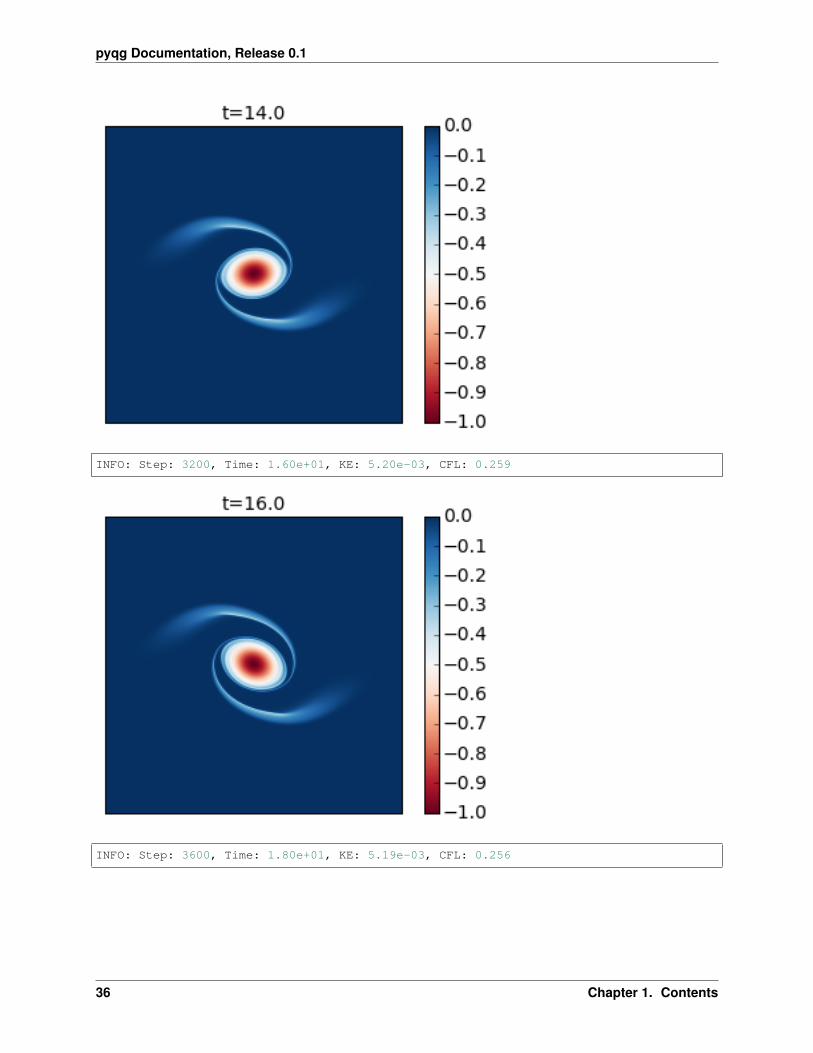
pyqg Documentation, Release 0.1
INFO: Step: 3200, Time: 1.60e+01, KE: 5.20e-03, CFL: 0.259
INFO: Step: 3600, Time: 1.80e+01, KE: 5.19e-03, CFL: 0.256
36 Chapter 1. Contents

pyqg Documentation, Release 0.1
INFO: Step: 4000, Time: 2.00e+01, KE: 5.19e-03, CFL: 0.259
INFO: Step: 4400, Time: 2.20e+01, KE: 5.19e-03, CFL: 0.259
1.3. Examples 37

pyqg Documentation, Release 0.1
INFO: Step: 4800, Time: 2.40e+01, KE: 5.18e-03, CFL: 0.242
INFO: Step: 5200, Time: 2.60e+01, KE: 5.17e-03, CFL: 0.263
38 Chapter 1. Contents

pyqg Documentation, Release 0.1
Compare these results with Figure 2 of the paper. In this simulation you see that as the cyclone rotates it develops thinarms that spread outwards and become unstable because of their strong shear. This is an excellent example of howsmaller scale vortices can be generated from a mesoscale vortex.
You can modify this to run it for longer time to generate the analogue of their Figure 3.
1.3.5 Built-in linear stability analysis
import numpy as npfrom numpy import piimport matplotlib.pyplot as plt%matplotlib inline
import pyqg
m = pyqg.LayeredModel(nx=256, nz = 2, U = [.01, -.01], V = [0., 0.], H = [1., 1.],L=2*pi,beta=1.5, rd=1./20., rek=0.05, f=1.,delta=1.)
INFO: Logger initializedINFO: Kernel initialized
To perform linear stability analysis, we simply call pyqg’s built-in method stability_analysis:
evals,evecs = m.stability_analysis()
The eigenvalues are stored in omg, and the eigenctors in evec. For plotting purposes, we use fftshift to reorder theentries
evals = np.fft.fftshift(evals.imag,axes=(0,))
k,l = m.k*m.radii[1], np.fft.fftshift(m.l,axes=(0,))*m.radii[1]
1.3. Examples 39

pyqg Documentation, Release 0.1
It is also useful to analyze the fasted-growing mode:
argmax = evals[m.Ny/2,:].argmax()evec = np.fft.fftshift(evecs,axes=(1))[:,m.Ny/2,argmax]kmax = k[m.Ny/2,argmax]
x = np.linspace(0,4.*pi/kmax,100)mag, phase = np.abs(evec), np.arctan2(evec.imag,evec.real)
By default, the stability analysis above is performed without bottom friction, but the stability method also supportsbottom friction:
evals_fric, evecs_fric = m.stability_analysis(bottom_friction=True)evals_fric = np.fft.fftshift(evals_fric.imag,axes=(0,))
argmax = evals_fric[m.Ny/2,:].argmax()evec_fric = np.fft.fftshift(evecs_fric,axes=(1))[:,m.Ny/2,argmax]kmax_fric = k[m.Ny/2,argmax]
mag_fric, phase_fric = np.abs(evec_fric), np.arctan2(evec_fric.imag,evec_fric.real)
Plotting growth rates
plt.figure(figsize=(14,4))plt.subplot(121)plt.contour(k,l,evals,colors='k')plt.pcolormesh(k,l,evals,cmap='Blues')plt.colorbar()plt.xlim(0,2.); plt.ylim(-2.,2.)plt.clim([0.,.1])plt.xlabel(r'$k \, L_d$'); plt.ylabel(r'$l \, L_d$')plt.title('without bottom friction')
plt.subplot(122)plt.contour(k,l,evals_fric,colors='k')plt.pcolormesh(k,l,evals_fric,cmap='Blues')plt.colorbar()plt.xlim(0,2.); plt.ylim(-2.,2.)plt.clim([0.,.1])plt.xlabel(r'$k \, L_d$'); plt.ylabel(r'$l \, L_d$')plt.title('with bottom friction')
<matplotlib.text.Text at 0x11539e290>
40 Chapter 1. Contents

pyqg Documentation, Release 0.1
plt.figure(figsize=(8,4))plt.plot(k[m.Ny/2,:],evals[m.Ny/2,:],'b',label='without bottom friction')plt.plot(k[m.Ny/2,:],evals_fric[m.Ny/2,:],'b--',label='with bottom friction')plt.xlim(0.,2.)plt.legend()plt.xlabel(r'$k\,L_d$')plt.ylabel(r'Growth rate')
<matplotlib.text.Text at 0x10f9731d0>
Plotting the wavestructure of the most unstable modes
plt.figure(figsize=(12,5))plt.plot(x,mag[0]*np.cos(kmax*x + phase[0]),'b',label='Layer 1')plt.plot(x,mag[1]*np.cos(kmax*x + phase[1]),'g',label='Layer 2')plt.plot(x,mag_fric[0]*np.cos(kmax_fric*x + phase_fric[0]),'b--')plt.plot(x,mag_fric[1]*np.cos(kmax_fric*x + phase_fric[1]),'g--')
1.3. Examples 41

pyqg Documentation, Release 0.1
plt.legend(loc=8)plt.xlabel(r'$x/L_d$'); plt.ylabel(r'$y/L_d$')
<matplotlib.text.Text at 0x114c6d410>
This calculation shows the classic phase-tilting of baroclinic unstable waves (e.g. Vallis 2006 ).
1.4 API
1.4.1 Base Model Class
This is the base class from which all other models inherit. All of these initialization arguments are available to all ofthe other model types. This class is not called directly.
class pyqg.Model(nz=1, nx=64, ny=None, L=1000000.0, W=None, dt=7200.0, twrite=1000.0,tmax=1576800000.0, tavestart=315360000.0, taveint=86400.0, useAB2=False,rek=5.787e-07, filterfac=23.6, f=None, g=9.81, diagnostics_list=’all’, ntd=1,log_level=1, logfile=None)
A generic pseudo-spectral inversion model.
42 Chapter 1. Contents

pyqg Documentation, Release 0.1
Attributes
nx, ny (int) Number of real space grid points in the x, y directions (cython)nk, nl (int) Number of spectal space grid points in the k, l directions (cython)nz (int) Number of vertical levels (cython)kk, ll (real array) Zonal and meridional wavenumbers (nk) (cython)a (real array) inversion matrix (nk, nk, nl, nk) (cython)q (real array) Potential vorticity in real space (nz, ny, nx) (cython)qh (complex array) Potential vorticity in spectral space (nk, nl, nk) (cython)ph (complex array) Streamfunction in spectral space (nk, nl, nk) (cython)u, v (real array) Zonal and meridional velocity anomalies in real space (nz, ny, nx) (cython)Ubg (real array) Background zonal velocity (nk) (cython)Qy (real array) Background potential vorticity gradient (nk) (cython)ufull, vfull (real arrays) Zonal and meridional full velocities in real space (nz, ny, nx) (cython)uh, vh (complex arrays) Velocity anomaly components in spectral space (nk, nl, nk) (cython)rek (float) Linear drag in lower layer (cython)t (float) Model time (cython)tc (int) Model timestep (cython)dt (float) Numerical timestep (cython)L, W (float) Domain length in x and y directionsfilterfac (float) Amplitdue of the spectral spherical filtertwrite (int) Interval for cfl writeout (units: number of timesteps)tmax (float) Total time of integration (units: model time)tavestart (float) Start time for averaging (units: model time)tsnapstart (float) Start time for snapshot writeout (units: model time)taveint (float) Time interval for accumulation of diagnostic averages. (units: model time)tsnapint (float) Time interval for snapshots (units: model time)ntd (int) Number of threads to use. Should not exceed the number of cores on your machine.pmodes (real array) Vertical pressure modes (unitless)radii ( real array) Deformation radii (units: model length)
Note: All of the test cases use nx==ny. Expect bugs if you choose these parameters to be different.
Note: All time intervals will be rounded to nearest dt interval.
Parameters nx : int
Number of grid points in the x direction.
ny : int
Number of grid points in the y direction (default: nx).
L : number
Domain length in x direction. Units: meters.
W :
Domain width in y direction. Units: meters (default: L).
rek : number
1.4. API 43
pyqg Documentation, Release 0.1
linear drag in lower layer. Units: seconds -1.
filterfac : number
amplitdue of the spectral spherical filter (originally 18.4, later changed to 23.6).
dt : number
Numerical timstep. Units: seconds.
twrite : int
Interval for cfl writeout. Units: number of timesteps.
tmax : number
Total time of integration. Units: seconds.
tavestart : number
Start time for averaging. Units: seconds.
tsnapstart : number
Start time for snapshot writeout. Units: seconds.
taveint : number
Time interval for accumulation of diagnostic averages. Units: seconds. (For perfor-mance purposes, averaging does not have to occur every timestep)
tsnapint : number
Time interval for snapshots. Units: seconds.
ntd : int
Number of threads to use. Should not exceed the number of cores on your machine.
describe_diagnostics()Print a human-readable summary of the available diagnostics.
modal_projection(p, forward=True)Performs a field p into modal amplitudes pn using the basis [pmodes]. The inverse transform calculates pfrom pn
run()Run the model forward without stopping until the end.
run_with_snapshots(tsnapstart=0.0, tsnapint=432000.0)Run the model forward, yielding to user code at specified intervals.
Parameters tsnapstart : int
The timestep at which to begin yielding.
tstapint : int
The interval at which to yield.
spec_var(ph)compute variance of p from Fourier coefficients ph
stability_analysis(bottom_friction=False)
Performs the baroclinic linear instability analysis given given the base state velocity :math: (U, V) andthe stretching matrix :math: S:
44 Chapter 1. Contents

pyqg Documentation, Release 0.1
𝐴Φ = 𝜔𝐵Φ,
where
𝐴 = 𝐵(𝑈𝑘 + 𝑉 𝑙) + 𝐼(𝑘𝑄𝑦 − 𝑙𝑄𝑥) + 1𝑗𝛿𝑁𝑁𝑟𝑒𝑘𝐼𝜅2
where 𝛿𝑁𝑁 = [0, 0, . . . , 0, 1],
and
𝐵 = 𝑆 − 𝐼𝜅2.
The eigenstructure is
Φ
and the eigenvalue is
‘𝜔‘
The growth rate is Im{𝜔}.
Parameters bottom_friction: optional inclusion linear bottom drag
in the linear stability calculation (default is False, as if :math: r_{ek} = 0)
Returns omega: complex array
The eigenvalues with largest complex part (units: inverse model time)
phi: complex array
The eigenvectors associated associated with omega (unitless)
vertical_modes()Calculate standard vertical modes. Simply the eigenvectors of the stretching matrix S
1.4.2 Specific Model Types
These are the actual models which are run.
class pyqg.QGModel(beta=1.5e-11, rd=15000.0, delta=0.25, H1=500, U1=0.025, U2=0.0, **kwargs)Two layer quasigeostrophic model.
This model is meant to representflows driven by baroclinic instabilty of a base-state shear 𝑈1 − 𝑈2. The upperand lower layer potential vorticity anomalies 𝑞1 and 𝑞2 are
𝑞1 = ∇2𝜓1 + 𝐹1(𝜓2 − 𝜓1)
𝑞2 = ∇2𝜓2 + 𝐹2(𝜓1 − 𝜓2)
with
𝐹1 ≡ 𝑘2𝑑1 + 𝛿2
𝐹2 ≡ 𝛿𝐹1 .
The layer depth ratio is given by 𝛿 = 𝐻1/𝐻2. The total depth is 𝐻 = 𝐻1 +𝐻2.
The background potential vorticity gradients are
𝛽1 = 𝛽 + 𝐹1(𝑈1 − 𝑈2)
𝛽2 = 𝛽 − 𝐹2(𝑈1 − 𝑈2) .
1.4. API 45

pyqg Documentation, Release 0.1
The evolution equations for 𝑞1 and 𝑞2 are
𝜕𝑡 𝑞1 + 𝐽(𝜓1 , 𝑞1) + 𝛽1 𝜓1𝑥 = ssd
𝜕𝑡 𝑞2 + 𝐽(𝜓2 , 𝑞2) + 𝛽2 𝜓2𝑥 = −𝑟𝑒𝑘∇2𝜓2 + ssd .
where ssd represents small-scale dissipation and 𝑟𝑒𝑘 is the Ekman friction parameter.
Parameters beta : number
Gradient of coriolis parameter. Units: meters -1 seconds -1
rek : number
Linear drag in lower layer. Units: seconds -1
rd : number
Deformation radius. Units: meters.
delta : number
Layer thickness ratio (H1/H2)
U1 : number
Upper layer flow. Units: m/s
U2 : number
Lower layer flow. Units: m/s
set_U1U2(U1, U2)Set background zonal flow.
Parameters U1 : number
Upper layer flow. Units: m/s
U2 : number
Lower layer flow. Units: m/s
set_q1q2(q1, q2, check=False)Set upper and lower layer PV anomalies.
Parameters q1 : array-like
Upper layer PV anomaly in spatial coordinates.
q1 : array-like
Lower layer PV anomaly in spatial coordinates.
class pyqg.LayeredModel(g=9.81, beta=1.5e-11, nz=4, rd=15000.0, H=None, U=None, V=None,rho=None, delta=None, **kwargs)
Layered quasigeostrophic model.
This model is meant to represent flows driven by baroclinic instabilty of a base-state shear. The potentialvorticity anomalies qi are related to the streamfunction psii through
𝑞𝑖 = ∇2𝜓𝑖 +𝑓20𝐻𝑖
(𝜓𝑖−1 − 𝜓𝑖
𝑔′𝑖−1
− 𝜓𝑖 − 𝜓𝑖+1
𝑔′𝑖
), 𝑖 = 2,N − 1 ,
𝑞1 = ∇2𝜓1 +𝑓20𝐻1
(𝜓2 − 𝜓1
𝑔′1
), 𝑖 = 1 ,
𝑞N = ∇2𝜓N +𝑓20𝐻N
(𝜓N−1 − 𝜓N
𝑔′N
)+
𝑓0𝐻N
ℎ𝑏 , 𝑖 = N ,
46 Chapter 1. Contents

pyqg Documentation, Release 0.1
where the reduced gravity, or buoyancy jump, is
𝑔′𝑖 ≡ 𝑔𝜌𝑖+1 − 𝜌𝑖
𝜌𝑖.
The evolution equations are
𝑞𝑖𝑡 + J (𝜓𝑖 , 𝑞𝑖) + Q𝑦𝜓𝑖𝑥 − Q𝑥𝜓𝑖𝑦 = ssd − 𝑟𝑒𝑘𝛿𝑖N∇2𝜓𝑖 , 𝑖 = 1,N ,
where the mean potential vorticy gradients are
Q𝑥 = SV ,
and
Q𝑦 = 𝛽 I − SU ,
where S is the stretching matrix, I is the identity matrix, and the background velocity is
V(𝑧) = (U,V).
Parameters nz : integer number
Number of layers (> 1)
beta : number
Gradient of coriolis parameter. Units: meters -1 seconds -1
rd : number
Deformation radius. Units: meters. Only necessary for the two-layer (nz=2) case.
delta : number
Layer thickness ratio (H1/H2). Only necessary for the two-layer (nz=2) case. Unitless.
U : list of size nz
Base state zonal velocity. Units: meters s -1
V : array of size nz
Base state meridional velocity. Units: meters s -1
H : array of size nz
Layer thickness. Units: meters
rho: array of size nz.
Layer density. Units: kilograms meters -3
class pyqg.BTModel(beta=0.0, rd=0.0, H=1.0, U=0.0, **kwargs)Single-layer (barotropic) quasigeostrophic model. This class can represent both pure two-dimensional flow andalso single reduced-gravity layers with deformation radius rd.
The equivalent-barotropic quasigeostrophic evolution equations is
𝜕𝑡𝑞 + 𝐽(𝜓, 𝑞) + 𝛽𝜓𝑥 = ssd
The potential vorticity anomaly is
𝑞 = ∇2𝜓 − 𝜅2𝑑𝜓
1.4. API 47

pyqg Documentation, Release 0.1
Parameters beta : number, optional
Gradient of coriolis parameter. Units: meters -1 seconds -1
rd : number, optional
Deformation radius. Units: meters.
U : number, optional
Upper layer flow. Units: meters.
set_U(U)Set background zonal flow.
Parameters U : number
Upper layer flow. Units meters.
class pyqg.SQGModel(beta=0.0, Nb=1.0, rd=0.0, H=1.0, U=0.0, **kwargs)Surface quasigeostrophic model.
Parameters beta : number
Gradient of coriolis parameter. Units: meters -1 seconds -1
Nb : number
Buoyancy frequency. Units: seconds -1.
U : number
Background zonal flow. Units: meters.
set_U(U)Set background zonal flow
1.4.3 Lagrangian Particles
class pyqg.LagrangianParticleArray2D(x0, y0, periodic_in_x=False, periodic_in_y=False,xmin=-inf, xmax=inf, ymin=-inf, ymax=inf, parti-cle_dtype=’f8’)
A class for keeping track of a set of lagrangian particles in two-dimensional space. Tries to be fast.
Parameters x0, y0 : array-like
Two arrays (same size) representing the particle initial positions.
periodic_in_x : bool
Whether the domain wraps in the x direction.
periodic_in_y : bool
Whether the domain ‘wraps’ in the y direction.
xmin, xmax : numbers
Maximum and minimum values of x coordinate
ymin, ymax : numbers
Maximum and minimum values of y coordinate
particle_dtype : dtype
Data type to use for particles
48 Chapter 1. Contents

pyqg Documentation, Release 0.1
step_forward_with_function(uv0fun, uv1fun, dt)Advance particles using a function to determine u and v.
Parameters uv0fun : function
Called like uv0fun(x,y). Should return the velocity field u, v at time t.
uv1fun(x,y) : function
Called like uv1fun(x,y). Should return the velocity field u, v at time t + dt.
dt : number
Timestep.
class pyqg.GriddedLagrangianParticleArray2D(x0, y0, Nx, Ny, grid_type=’A’, **kwargs)Lagrangian particles with velocities given on a regular cartesian grid.
Parameters x0, y0 : array-like
Two arrays (same size) representing the particle initial positions.
Nx, Ny: int
Number of grid points in the x and y directions
grid_type: {‘A’}
Arakawa grid type specifying velocity positions.
interpolate_gridded_scalar(x, y, c, order=1, pad=1, offset=0)Interpolate gridded scalar C to points x,y.
Parameters x, y : array-like
Points at which to interpolate
c : array-like
The scalar, assumed to be defined on the grid.
order : int
Order of interpolation
pad : int
Number of pad cells added
offset : int
???
Returns ci : array-like
The interpolated scalar
step_forward_with_gridded_uv(U0, V0, U1, V1, dt, order=1)Advance particles using a gridded velocity field. Because of the Runga-Kutta timestepping, we need twovelocity fields at different times.
Parameters U0, V0 : array-like
Gridded velocity fields at time t - dt.
U1, V1 : array-like
Gridded velocity fields at time t.
dt : number
1.4. API 49
pyqg Documentation, Release 0.1
Timestep.
order : int
Order of interpolation.
1.4.4 Diagnostic Tools
pyqg.diagnostic_tools.calc_ispec(model, ph)Compute isotropic spectrum phr of ph from 2D spectrum.
Parameters model : pyqg.Model instance
The model object from which ph originates
ph : complex array
The field on which to compute the variance
Returns kr : array
isotropic wavenumber
phr : array
isotropic spectrum
pyqg.diagnostic_tools.spec_sum(ph2)Compute total spectral sum of the real spectral quantity‘‘ph^2‘‘.
Parameters model : pyqg.Model instance
The model object from which ph originates
ph2 : real array
The field on which to compute the sum
Returns var_dens : float
The sum of ph2
pyqg.diagnostic_tools.spec_var(model, ph)Compute variance of p from Fourier coefficients ph.
Parameters model : pyqg.Model instance
The model object from which ph originates
ph : complex array
The field on which to compute the variance
Returns var_dens : float
The variance of ph
1.5 Development
1.5.1 Team
• Malte Jansen, University of Chicago
• Ryan Abernathey, Columbia University / LDEO
50 Chapter 1. Contents

pyqg Documentation, Release 0.1
• Cesar Rocha, Scripps Institution of Oceanography / UCSD
• Francis Poulin, University of Waterloo
1.5.2 History
The numerical approach of pyqg was originally inspired by a MATLAB code by Glenn Flierl of MIT, who was ateacher and mentor to Ryan and Malte. It would be hard to find anyone in the world who knows more about this sortof model than Glenn. Malte implemented a python version of the two-layer model while at GFDL. In the summer of2014, while both were at the WHOI GFD Summer School, Ryan worked with Malte refactor the code into a properpython package. Cesar got involved and brought pyfftw into the project. Ryan implemented a cython kernel. Cesarand Francis implemented the barotropic and sqg models.
1.5.3 Future
By adopting open-source best practices, we hope pyqg will grow into a widely used, communited-based project. Weknow that many other research groups have their own “in house” QG models. You can get involved by trying out themodel, filing issues if you find problems, and making pull requests if you make improvements.
1.5.4 Develpment Workflow
Anyone interested in helping to develop pyqg needs to create their own fork of our git repository. (Follow the githubforking instructions. You will need a github account.)
Clone your fork on your local machine.
$ git clone [email protected]:USERNAME/pyqg
(In the above, replace USERNAME with your github user name.)
Then set your fork to track the upstream pyqg repo.
$ cd pyqg$ git remote add upstream git://github.com/pyqg/pyqg.git
You will want to periodically sync your master branch with the upstream master.
$ git fetch upstream$ git rebase upstream/master
Never make any commits on your local master branch. Instead open a feature branch for every new development task.
$ git checkout -b cool_new_feature
(Replace cool_new_feature with an appropriate description of your feature.) At this point you work on your newfeature, using git add to add your changes. When your feature is complete and well tested, commit your changes
$ git commit -m 'did a bunch of great work'
and push your branch to github.
$ git push origin cool_new_feature
1.5. Development 51

pyqg Documentation, Release 0.1
At this point, you go find your fork on github.com and create a pull request. Clearly describe what you have done inthe comments. If your pull request fixes an issue or adds a useful new feature, the team will gladly merge it.
After your pull request is merged, you can switch back to the master branch, rebase, and delete your feature branch.You will find your new feature incorporated into pyqg.
$ git checkout master$ git fetch upstream$ git rebase upstream/master$ git branch -d cool_new_feature
1.5.5 Virtual Environment
This is how to create a virtual environment into which to test-install pyqg, install it, check the version, and tear downthe virtual environment.
$ conda create --yes -n test_env python=2.7 pip nose numpy cython scipy nose$ conda install --yes -n test_env -c nanshe pyfftw$ source activate test_env$ pip install pyqg$ python -c 'import pyqg; print(pyqg.__version__);'$ source deactivate$ conda env remove --yes -n test_env
1.5.6 Release Procedure
Once we are ready for a new release, someone needs to make a pull request which updates the version number insetup.py. Also make sure that whats-new.rst in the docs is up to date.
After the new version number PR has been merged, create a new release in github.
The step of publishing to pypi has to be done manually from the command line. (Note: I figured out how this worksfrom these instructions). After the new release has been created, do the following.
$ cd pyqg$ git fetch upstream$ git checkout master$ git rebease upstream/master# test the release before publishing$ python setup.py register -r pypitest$ python setup.py sdist upload -r pypitest# if that goes well, publish it$ python setup.py register -r pypi$ python setup.py sdist upload -r pypi
Note that pypi will not let you publish the same release twice, so make sure you get it right!
1.6 What’s New
1.6.1 v0.2.0 (27 April 2016)
Added compatibility with python 3.
Implemented linear baroclinic stability analysis method.
52 Chapter 1. Contents

pyqg Documentation, Release 0.1
Implemented vertical mode methods and modal KE and PE spectra diagnostics.
Implemented multi-layer subclass.
Added new logger that leverages on built-in python logging.
Changed license to MIT.
1.6.2 v0.1.4 (22 Oct 2015)
Fixed bug related to the sign of advection terms (GH86).
Fixed bug in _calc_diagnostics (GH75). Now diagnostics start being averaged at tavestart.
1.6.3 v0.1.3 (4 Sept 2015)
Fixed bug in setup.py that caused openmp check to not work.
1.6.4 v0.1.2 (2 Sept 2015)
Package was not building properly through pip/pypi. Made some tiny changes to setup script. pypi forces you toincrement the version number.
1.6.5 v0.1.1 (2 Sept 2015)
A bug-fix release with no api or feature changes. The kernel has been modified to support numpy fft routines.
• Removed pyfftw depenency (GH53)
• Cleaning of examples
1.6.6 v0.1 (1 Sept 2015)
Initial release.
1.6. What’s New 53

pyqg Documentation, Release 0.1
54 Chapter 1. Contents

Python Module Index
ppyqg, 42pyqg.diagnostic_tools, 50
55

pyqg Documentation, Release 0.1
56 Python Module Index
Index
BBTModel (class in pyqg), 47
Ccalc_ispec() (in module pyqg.diagnostic_tools), 50
Ddescribe_diagnostics() (pyqg.Model method), 44
GGriddedLagrangianParticleArray2D (class in pyqg), 49
Iinterpolate_gridded_scalar()
(pyqg.GriddedLagrangianParticleArray2Dmethod), 49
LLagrangianParticleArray2D (class in pyqg), 48LayeredModel (class in pyqg), 46
Mmodal_projection() (pyqg.Model method), 44Model (class in pyqg), 42
Ppyqg (module), 42pyqg.diagnostic_tools (module), 50
QQGModel (class in pyqg), 45
Rrun() (pyqg.Model method), 44run_with_snapshots() (pyqg.Model method), 44
Sset_q1q2() (pyqg.QGModel method), 46
set_U() (pyqg.BTModel method), 48set_U() (pyqg.SQGModel method), 48set_U1U2() (pyqg.QGModel method), 46spec_sum() (in module pyqg.diagnostic_tools), 50spec_var() (in module pyqg.diagnostic_tools), 50spec_var() (pyqg.Model method), 44SQGModel (class in pyqg), 48stability_analysis() (pyqg.Model method), 44step_forward_with_function()
(pyqg.LagrangianParticleArray2D method), 48step_forward_with_gridded_uv()
(pyqg.GriddedLagrangianParticleArray2Dmethod), 49
Vvertical_modes() (pyqg.Model method), 45
57


