International Journal of Science and Research (IJSR) ISSN: 2319-7064

ResearchGate Impact Factor (2018): 0.28 | SJIF (2018): 7.426

Volume 8 Issue 10, October 2019

www.ijsr.net Licensed Under Creative Commons Attribution CC BY

q- Continuity Equation

Amna Hasan

Department of Mathematics, College of Sciences, Albaha University, KSA. Department of Mathematics, Al neelain University, Sudan

Abstract: For 𝒒 ∈ 𝟎, 𝟏 , a 𝒒 − deformation of the continuity equation is introduced using the q- derivative (or Jackson derivative). By

quantum calculus, we solve these equations.

Keywords: 𝑞 − derivative, 𝑞 − continuity equation.

1. Introduction

A continuity equation in physics is an equation that

describes the transport of some quantity. It is particularly

simple and powerful when applied to a conserved quantity,

but it can be generalized to apply to any extensive quantity.

Since mass, energy, momentum, electric charge and other

natural quantities are conserved under their respective

appropriate conditions, a variety of physical phenomena may

be described using continuity equations. Continuity

equations are a stronger, local form of conservation laws.

For example, a weak version of the law of conservation of

energy states that energy can neither be created nor

destroyed i.e., the total amount of energy in the universe is

fixed. This statement does not rule out the possibility that a

quantity of energy could disappear from one point while

simultaneously appearing at another point. A stronger

statement is that energy is locally conserved: energy can

neither be created nor destroyed, nor can it ”teleport” from

one place to another, it can only move by a continuous

flow.Acontinuityequationisthemathematicalwaytoexpressthis

kindofstatement. For example, the continuity equation for

electric charge states that the amount of electric charge in

any volume of space can only change by the amount of

electric current flowing into or out of that volume through its

boundaries. An alternative expression of the continuity

equation for a species in the atmosphere can be derived

relative to a frame reference moving with the local flow; this

is called the Lagrangian approach. Consider a fluid element

at location 𝑋0 at time 𝑡. We wish to know where this element

will be located at a later time 𝑡. We define a transition

probability density such that the probability that the fluid

element will have moved to within a volume

𝑑𝑥, 𝑑𝑦, 𝑑𝑧 centered at location X at time t. Continuity

equations more generally can include “source” and “sink”

terms, which allow them to describe quantities that are often

but not always conserved, such as the density of a molecular

species which can be created or destroyed by chemical

reactions. In an everyday example, there is a continuity

equation for the number of people alive; it has a ”source

term” to account for people being born, and a ”sink term” to

account for people dying.

Any continuity equation can be expressed in an ”integral

form” in terms of a flux integral, which applies to any finite

region, or in a differential form interms of the divergence

operator) which applies at a point. Continuity equations

underlie more specific transport equations such as the

convection diffusion equation, Boltzmann transport

equation, and Navier-Stokes equations.

A continuity equation is useful when a flux can be defined.

To define flux, first there must be a quantity 𝑄 which can

flow or move, such as mass, energy, electric charge,

momentum, number of molecules, etc. Let 𝜌 be the volume

density of this quantity, that is, the amount of 𝑄 per unit

volume.

By the divergence theorem, a general continuity equation

can also be written in a differential form:

where ∇ is divergence, 𝜌 is the amount of the quantity 𝑄 per

unit volume, 𝑗 is the flux of 𝑄, 𝑡 is time, 𝜎 is the generation

of 𝑄 per unit volume per unit time. Terms that generate 𝑄

(i.e. 𝜎 > 0) or remove 𝑄 (i.e. 𝜎 < 0) are referred to as a

”sources” and ”sinks” respectively. This general equation

may be used to derive any continuity equation, ranging from

as simple as the volume continuity equation to as

complicated as the Navier-Stokes equations. This equation

also generalizes the advection equation. Other equations in

physics, such as Gauss’s law of the electric field and Gauss’s

law for gravity, have a similar mathematical form to the

continuity equation, but are not usually referred to by the

term ”continuity equation”, because j in those cases does not

represent the flow of a real physical quantity. In the case that

𝑄 is a conserved quantity that cannot be created or destroyed

(such as energy), 𝜎 = 0 and the equations becomes:

In electromagnetic theory, the continuity equation is an

empirical law expressing (local) charge conservation.

Mathematically it is an automatic consequence of Maxwell’s

equations, although charge conservation is more

fundamental than Maxwell’s equations. It states that the

divergence of the current density 𝑗 (in amperes per square

meter) is equal to the negative rate of change of the charge

density 𝜌 (in coulombs per cubic metre),

Current is the movement of charge. The continuity equation

says that if charge is moving out of a differential volume

(i.e. divergence of current density is positive) then the

amount of charge within that volume is going to decrease, so

the rate of change of charge density is negative. Therefore,

the continuity equation amounts to a conservation of charge.

If magnetic monopoles exist, there would be a continuity

equation for monopole currents as well, see the monopole

article for background and the duality between electric and

magnetic currents. In fluid dynamics, the continuity equation

Paper ID: ART20201322 10.21275/ART20201322 500

International Journal of Science and Research (IJSR) ISSN: 2319-7064

ResearchGate Impact Factor (2018): 0.28 | SJIF (2018): 7.426

Volume 8 Issue 10, October 2019

www.ijsr.net Licensed Under Creative Commons Attribution CC BY

states that the rate at which mass enters a system is equal to

the rate at which mass leaves the system plus the

accumulation of mass within the system. Conservation of

energy says that energy cannot be created or destroyed. (See

below for the nuances associated with general relativity.)

Therefore, there is a continuity equation for energy flow:

Where 𝑢 is a local energy density (energy per unit volume),

𝑄 is energy flux (transfer of energy per unit cross-sectional

area per unit time) as a vector. An important practical

example is the flow of heat. When heat flows inside a solid,

the continuity equation can be combined with Fourier’s law

(heat flux is proportional to temperature gradient) to arrive at

the heat equation. The equation of heat flow mayalso have

source terms: although energy cannot becreated or

destroyed, heat can be created from other types of energy,

for example via friction or joule heating.

In recent years the q-deformation of the Heisemburg

commutation relation has drawn attention. In the paper [10],

the purpose was to understand the probability distribution of

a non-commutative random variable 𝑎 + 𝑎∗, where 𝑎 is a

bounded operator on some Hilbert space satisfying

for some 𝑞 ∈ [−1,1). The calculation is inspired by the case,

𝑞 = 0, where 𝑎 and 𝑎∗, turn out to be the left and right shift

on 𝑙2(ℕ), In this case a and 𝑎∗, can be quite nicely

represented as operators on the Hardy class ℋ2of all

analytic functions on the unit disk with 𝐿2 limits toward the

boundary.

Subsequently, they find a measure 𝜇𝑞 , 𝑞 ∈ −1,1 , on the

complex plane that replaces the Lebesgue measure on the

unit circle in the above: µq is concentrated on a family of

concentric circle, the largest of which has the radius1

1−𝑞 .

Their representation space (see[10]) will be ℌ2 𝔇𝑞 , 𝜇𝑞 the

completion of the analytic functions on ℑ𝑞 = 𝑧 ∈ ℂ 𝑧 2 <

11−𝑞 (1−q)}with respect to the inner product defined by𝜇𝑞.

In this space annihilation operator 𝑎 is represented by a 𝑞

difference operator 𝐷𝑞 . As 𝑞 tends to 1, 𝜇𝑞will tend to the

Gauss measure on ℂ and 𝐷𝑞 becomes differentiation. So, it is

natural to ask what is the 𝑞 - deformation of the continuity

equation. This paper organized as follows. In Section 2, we

briefly recall well-known results on 𝑞 - calculus, Jackson

derivative (or 𝑞 -derivative) and useful representations. In

Section 3, we introduce 𝑞 -continuity equation and we

deduced some theorems.

2. Preliminaries

We recall some basic notations of the language of q-calculus

(see [1, 2, 7, 9, 10]). The natural number n has the following

q deformation:

𝑛 𝑞 ≔ 1 + 𝑞 + 𝑞2 + ∙ ∙ ∙ +𝑞𝑛−1, with 0 𝑞 = 0.

Occasionally we shall write ∞ 𝑞 for the limit of these

numbers: 1

1−𝑞 . The 𝑞 factorials and 𝑞 binomial coefficients

are defined naturally as

𝑛 𝑞 ! ≔ 1 𝑞 ∙ 2 𝑞 ⋯ 𝑛 𝑞 with 0 𝑞 ≔ 1

Recall that from [10], for 𝑞 ∈ (−1,1). relation (1) admits,

up to unitary equivalence, a unique non-trivial bounded

irreducible representation given on the canonical basis 𝑒𝑛 𝑛 ∈ ℕ of 𝑙2(ℕ)by:

For 𝑞 ∈ (0,1) and analytic 𝑓: ℂ ⟶ ℂdefine operators 𝑍 and

𝐷𝑞 as follows (see [7, 9, 10])

The operator𝐷𝑞 has the following properties:

It is well known ([10]) that the operators 𝐷𝑞 and 𝑍 give a

bounded representation of (1), i.e., 𝐷𝑞 and 𝑍 satisfy

With respect to the measure (see [10])

where 𝜆𝑟𝑘

is the normalized Lebesgue measure on the circle

with radius𝑟𝑘 , they define the inner product

for all 𝑓, 𝑔 ∈ ℌ2 𝔇𝑞 , 𝜇𝑞 . Note that 𝜇𝑞 ⟶ 𝜇0 when 𝑞 ⟶ 0,

where 𝜇0 is the normalized Lebsgue measure on the unit

circle and that, in the limit 𝑞 ↑ 1,𝜇𝑞 tends to the Gauss

measure on the complex plane. The identification 𝑎 = 𝐷𝑞and

𝑎∗ = 𝑍 determine a representation of (1) on ℌ2 𝔇𝑞 , 𝜇𝑞 . In

particular, with 𝑒𝑛 ≔ 𝑧𝑛 , (i),(ii) and (iii) are satisfied, and

therefore 𝐷𝑞∗ = 𝑍. For more details see Ref. [10].

3. q-Continuity Equation

Let 𝑞 ∈ (0,1). Recall that

And

Paper ID: ART20201322 10.21275/ART20201322 501

International Journal of Science and Research (IJSR) ISSN: 2319-7064

ResearchGate Impact Factor (2018): 0.28 | SJIF (2018): 7.426

Volume 8 Issue 10, October 2019

www.ijsr.net Licensed Under Creative Commons Attribution CC BY

As a 𝑞-deformation of the continuity equation

we will study the following equation

Theorem3.1. For 𝑞 ∈ (0,1), the q-continuity equation (4)

gives

Proof: From equation (2) we get

.

.

.

Then, we obtain

Therefore, we deduce that

As𝑘 → ∞ we get

which completes the proof.

Theorem3.2. For 𝑞 ∈ (0,1), the solution of the 𝑞 -

continuity equation (4) is given by

Proof: From equation (2) we get

Which gives

.

.

.

Then, we get

.

.

.

Then, we obtain

As𝑘 → ∞ we get

as desired.

References

[1] W. H. Abdi, On certain q-difference equations and q-

Laplace transforms, Proc. Nat. Inst. Sci. India Acad , 28

A, pp. 1-15, (1962).

[2] C. R. Adams, On the linear ordinary q-difference

equation, Am. Math. Ser., II, 30, pp. 195-205, (1929).

[3] Sami.H.Altoum,q-

deformationofTransonicGasEquation,JournalofMathem

aticsandStatistics,14(2018),88-93.

[4] Sami. H. Altoum, q-deformation of Transonic Gas

Equation, American Journal of Applied Sciences, 15

(2018), 261-266.

[5] S. H. Altoum., H. A. Othman, H. Rguigui, Quantum

white noise Gaussian kernel operators, Chaos, Solitons

& Fractals, 104 (2017), 468-476.

[6] G. Bangerezako, Varitional q-calculus, J. Math. Anal.

Appl. , 289, pp. 650-665, (2004).

[7] G. Gasper and M. Rahman, Basic hypergeometric

series. Vol 35 of Encyclopedia Of Mathematics And Its

Application, Cambridge Universty Press, Cambridge

(1990). [8] I. M. Gel’fand and G. E. Shilov, Generalized

Functions, Vol.I. Academic Press, Inc., New York,

1968.

[8] H. F. Jackson, q-Difference equations, Am. J. Math., 32,

pp. 305-314, (1910).

[9] H. V. Leeuwen and H. Maassen, A q-deformation of the

Gauss distribution. Journal of mathematical physic

36(9), 4743-4756 (1995).

[10] T. E. Mason, On properties of the solution of linear q-

difference equations with entire function coeffcients,

Am. J. Math., 37 , pp. 439-444, (1915).

[11] P. Protter, Stochastic integration and Differential

equations , A New Approach. Springer, Berlin, (1992).

[12] H. Rguigui, Quantum Ornstein-Uhlenbeck semigroups,

Qunantum Studies: Math. and Foundations, 2, 159-175,

(2015).

Paper ID: ART20201322 10.21275/ART20201322 502

International Journal of Science and Research (IJSR) ISSN: 2319-7064

ResearchGate Impact Factor (2018): 0.28 | SJIF (2018): 7.426

Volume 8 Issue 10, October 2019

www.ijsr.net Licensed Under Creative Commons Attribution CC BY

[13] H. Rguigui, Quantum λ-potentials associated to

quantum Ornstein - Uhlenbeck semigroups, Chaos,

Solitons & Fractals, Vol. 73, 80-89, (2015).

[14] H. Rguigui, Characterization of the QWN-conservation

operator, Chaos, Solitons & Fractals, Volume 84, 41-48,

(2016).

[15] H.Rguigui,WickDifferentialandPoissonEquationsAssoci

atedToTheQWN-EulerOperatorActingOnGeneralized

Operators, Mathematica Slo., 66 (2016), No. 6, 1487-

1500.

[16] H. Rguigui, Fractional Number Operator and

Associated Fractional Diffusion Equations, Math Phys

Anal Geom, 21:1-17, (2018).

[17] H. Rguigui, Characterization Theorems for the

Quantum White Noise Gross Laplacian and

Applications,Complex Anal. Oper. Theory, 12:1637-

1656, (2018).

[18] R. Rundnicki, K. Pichor and M. Tyran-Kaminska,

Markov semigroups and their applications, Dynamics of

Dissipation, Volume 597 of the series Lecture Notes in

Physics pp. 215-238, Springer Berlin Heidelberg

(2002).

Paper ID: ART20201322 10.21275/ART20201322 503

POSTER PRESENTATION Open Access

Continuity equation-derived valve area usingCMR phase-contrast provides flow-independentassessment of valve stenosisKevin Gralewski1*, Walter R Witschey2, Sam D Pollock1, Kevin K Whitehead1

From 19th Annual SCMR Scientific SessionsLos Angeles, CA, USA. 27-30 January 2016

BackgroundAssessing aortic valve stenosis (AVS) by cardiac magneticresonance (CMR) remains challenging, largely due toeffects of accelerated flow and resulting pressure recovery,or the phenomena of kinetic energy transmuting to staticfluid pressure distally. Effective orifice area (EOA) is atechnique used in echocardiography and has been shownto improve AVS assessment. The potential of phase-contrast velocity mapping (PC-MRI) to improve the accu-racy of EOA rests on the ability to resolve high peakvelocities; previous studies have shown systematic under-estimation compared to echocardiography. We used invitro experiments to assess the accuracy of EOA using thecontinuity equation with PC-MRI derived peak velocitiesand flows.

MethodsA custom flow phantom, 20 mm in diameter, was createdby 3D printing to mimic AVS by either a 6 mm diameter(D) orifice plate or casted polyurethane bicuspid AV(bAV). Pressure taps were set on the phantom at 20 mm,or 1D, either side of the plate/bAV, 2.5D proximally, and8D distally. A 40% glycerin-aqueous solution was deliveredin various steady-state and pulsatile profiles by an MRI-compatible pump (Shelley Medical Imagining, Ontario,Canada). Pressures were measured by clinical transducers(Edwards Scientific, Washington DC). PC-MRI assessedflow: in-plane acquisitions identified the region of maximalvelocity, whereupon optimized through-plane (TR 40msec, TE 2.3-2.4 ms, 25° flip angle, 1.5 × 1.5 × 4.5 mm)determined peak velocity and flow, the latter taken justproximal to AVS. All PC-MRI data was obtained on

Siemens 1.5T Avanto scanner and analyzed by CVI42(Circle Cardiovascular Imaging, Calgary). EOA in eachtrial was calculated by the continuity equation (EOA =Peak Flow Rate / Peak Velocity).

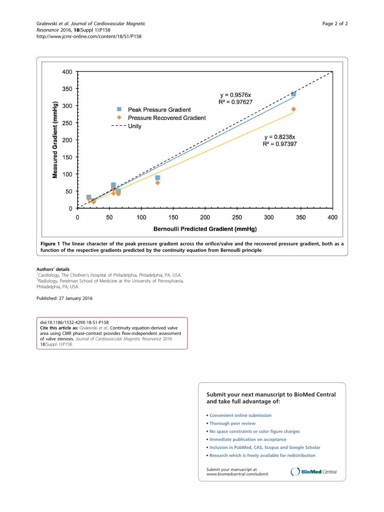
ResultsPC-measured average flow rates showed good agreementwith programmed Flow rates (SD = 0.07, p < 0.0005). TheBernoilli-derived predicted gradients demonstrated excel-lent agreement with the measured peak gradient. How-ever, it overestimated the gradient as expected due topressure recovery. The calculated EOAs were consistentwith the physical dimension of the plate/bAV and wasflow-rate independent. Conversely, both pressure gradientand pressure recovery were directly related to peak velo-city as expected (R2= 0.976, p < 0.001; R2= 0.946,p < 0.001, respectively, see Fig). Pressure recovery in theplate was also noted to be consistently higher than predic-tions from previous reports, though this trend did nothold for the bAV trials.

ConclusionsPC-MR technique can provide accurate peak velocity mea-surements over a wide range of gradients provided TE isappropriately minimized. As such, PC-MR may provideaccurate EOA that is flow-rate independent. Pressurerecovery appears multifactorial, though flow and geometryof stenosis seem to be the most significant. PC-MRIderived EOA is a promising technique that may providemore reliable quantification of valve stenosis than echocar-diography due to more accurate flow measurement andless variability.

1Cardiology, The Chidlren’s Hospital of Philadelphia, Philadelphia, PA, USAFull list of author information is available at the end of the article

Gralewski et al. Journal of Cardiovascular MagneticResonance 2016, 18(Suppl 1):P158http://www.jcmr-online.com/content/18/S1/P158

© 2016 Gralewski et al. This is an Open Access article distributed under the terms of the Creative Commons Attribution License (http://creativecommons.org/licenses/by/4.0), which permits unrestricted use, distribution, and reproduction in any medium, provided theoriginal work is properly cited. The Creative Commons Public Domain Dedication waiver (http://creativecommons.org/publicdomain/zero/1.0/) applies to the data made available in this article, unless otherwise stated.

Authors’ details1Cardiology, The Chidlren’s Hospital of Philadelphia, Philadelphia, PA, USA.2Radiology, Perelman School of Medicine at the University of Pennsylvania,Philadelphia, PA, USA.

Published: 27 January 2016

doi:10.1186/1532-429X-18-S1-P158Cite this article as: Gralewski et al.: Continuity equation-derived valvearea using CMR phase-contrast provides flow-independent assessmentof valve stenosis. Journal of Cardiovascular Magnetic Resonance 201618(Suppl 1):P158.

Submit your next manuscript to BioMed Centraland take full advantage of:

• Convenient online submission

• Thorough peer review

• No space constraints or color figure charges

• Immediate publication on acceptance

• Inclusion in PubMed, CAS, Scopus and Google Scholar

• Research which is freely available for redistribution

Submit your manuscript at www.biomedcentral.com/submit

Figure 1 The linear character of the peak pressure gradient across the orifice/valve and the recovered pressure gradient, both as afunction of the respective gradients predicted by the continuity equation from Bernoulli principle.

Gralewski et al. Journal of Cardiovascular MagneticResonance 2016, 18(Suppl 1):P158http://www.jcmr-online.com/content/18/S1/P158

Page 2 of 2

Continuity equationA continuity equation in physics is an equation that describes the transport of some quantity. It is particularlysimple and powerful when applied to a conserved quantity, but it can be generalized to apply to any extensivequantity. Since mass, energy, momentum, electric charge and other natural quantities are conserved under theirrespective appropriate conditions, a variety of physical phenomena may be described using continuityequations.

Continuity equations are a stronger, local form of conservation laws. For example, a weak version of the lawof conservation of energy states that energy can neither be created nor destroyed—i.e., the total amount ofenergy in the universe is fixed. This statement does not rule out the possibility that a quantity of energy coulddisappear from one point while simultaneously appearing at another point. A stronger statement is that energyis locally conserved: energy can neither be created nor destroyed, nor can it "teleport" from one place toanother—it can only move by a continuous flow. A continuity equation is the mathematical way to express thiskind of statement. For example, the continuity equation for electric charge states that the amount of electriccharge in any volume of space can only change by the amount of electric current flowing into or out of thatvolume through its boundaries.

Continuity equations more generally can include "source" and "sink" terms, which allow them to describequantities that are often but not always conserved, such as the density of a molecular species which can becreated or destroyed by chemical reactions. In an everyday example, there is a continuity equation for thenumber of people alive; it has a "source term" to account for people being born, and a "sink term" to accountfor people dying.

Any continuity equation can be expressed in an "integral form" (in terms of a flux integral), which applies toany finite region, or in a "differential form" (in terms of the divergence operator) which applies at a point.

Continuity equations underlie more specific transport equations such as the convection–diffusion equation,Boltzmann transport equation, and Navier–Stokes equations.

Flows governed by continuity equations can be visualized using a Sankey diagram.

General equationDefinition of fluxIntegral formDifferential form

ElectromagnetismFluid dynamicsEnergy and heatProbability distributionsQuantum mechanicsRelativistic version

Special relativityGeneral relativity

Contents

Particle physicsNoether's theoremSee alsoReferencesFurther reading

A continuity equation is useful when a flux can be defined. To define flux, first there must be a quantity qwhich can flow or move, such as mass, energy, electric charge, momentum, number of molecules, etc. Let ρbe the volume density of this quantity, that is, the amount of q per unit volume.

The way that this quantity q is flowing is described by its flux. The flux of q is a vector field, which wedenote as j. Here are some examples and properties of flux:

The dimension of flux is "amount of q flowing per unit time, through a unit area". For example,in the mass continuity equation for flowing water, if 1 gram per second of water is flowingthrough a pipe with cross-sectional area 1 cm2, then the average mass flux j inside the pipe is(1 gram / second) / cm2, and its direction is along the pipe in the direction that the water isflowing. Outside the pipe, where there is no water, the flux is zero.If there is a velocity field u which describes the relevant flow—in other words, if all of thequantity q at a point x is moving with velocity u(x)—then the flux is by definition equal to thedensity times the velocity field:

For example, if in the mass continuity equation for flowing water, u is the water's velocity ateach point, and ρ is the water's density at each point, then j would be the mass flux.

In a well-known example, the flux of electric charge is the electric current density.

If there is an imaginary surface S, then the surface integral of flux over S is equal to the amountof q that is passing through the surface S per unit time:

in which ∬S dS is a surface integral.

(Note that the concept that is here called "flux" is alternatively termed "flux density" in some literature, inwhich context "flux" denotes the surface integral of flux density. See the main article on Flux for details.)

General equation

Definition of flux

Integral form

Illustration of how the flux j of a quantity q passes through anopen surface S. (dS is differential vector area).

In the integral form of the continuityequation, S is any closed surface thatfully encloses a volume V, like any of thesurfaces on the left. S can not be asurface with boundaries, like those on theright. (Surfaces are blue, boundaries arered.)

The integral form of the continuityequation states that:

The amount of q in a regionincreases when additional q flowsinward through the surface of theregion, and decreases when itflows outward;The amount of q in a regionincreases when new q is createdinside the region, and decreaseswhen q is destroyed;Apart from these two processes,there is no other way for theamount of q in a region to change.

Mathematically, the integral form of thecontinuity equation expressing the rate ofincrease of q within a volume V is:

where

S is any imaginary closed surface, that encloses avolume V,

dS denotes a surface integral over that closed

surface,q is the total amount of the quantity in the volume V,j is the flux of q,t is time,Σ is the net rate that q is being generated inside thevolume V per unit time. When q is being generated, itis called a source of q, and it makes Σ more positive.When q is being destroyed, it is called a sink of q, andit makes Σ more negative. This term is sometimeswritten as or the total change of q from itsgeneration or destruction inside the control volume.

In a simple example, V could be a building, and q could be thenumber of people in the building. The surface S would consist ofthe walls, doors, roof, and foundation of the building. Then thecontinuity equation states that the number of people in thebuilding increases when people enter the building (an inward

S

flux through the surface), decreases when people exit the building (an outward flux through the surface),increases when someone in the building gives birth (a source, Σ > 0), and decreases when someone in thebuilding dies (a sink, Σ < 0).

By the divergence theorem, a general continuity equation can also be written in a "differential form":

where

∇⋅ is divergence,ρ is the amount of the quantity q per unit volume,j is the flux of q,t is time,σ is the generation of q per unit volume per unit time. Terms that generate q (i.e. σ > 0) orremove q (i.e. σ < 0) are referred to as a "sources" and "sinks" respectively.

This general equation may be used to derive any continuity equation, ranging from as simple as the volumecontinuity equation to as complicated as the Navier–Stokes equations. This equation also generalizes theadvection equation. Other equations in physics, such as Gauss's law of the electric field and Gauss's law forgravity, have a similar mathematical form to the continuity equation, but are not usually referred to by the term"continuity equation", because j in those cases does not represent the flow of a real physical quantity.

In the case that q is a conserved quantity that cannot be created or destroyed (such as energy), σ = 0 and theequations become:

In electromagnetic theory, the continuity equation is an empirical law expressing (local) charge conservation.Mathematically it is an automatic consequence of Maxwell's equations, although charge conservation is morefundamental than Maxwell's equations. It states that the divergence of the current density J (in amperes persquare metre) is equal to the negative rate of change of the charge density ρ (in coulombs per cubic metre),

Consistency with Maxwell's equations

One of Maxwell's equations, Ampère's law (with Maxwell's correction),states that

Differential form

Electromagnetism

Taking the divergence of both sides (the divergence and partial derivativein time commute) results in

but the divergence of a curl is zero, so that

But Gauss's law (another Maxwell equation), states that

which can be substituted in the previous equation to yield the continuityequation

Current is the movement of charge. The continuity equation says that if charge is moving out of a differentialvolume (i.e. divergence of current density is positive) then the amount of charge within that volume is going todecrease, so the rate of change of charge density is negative. Therefore, the continuity equation amounts to aconservation of charge.

If magnetic monopoles exist, there would be a continuity equation for monopole currents as well, see themonopole article for background and the duality between electric and magnetic currents.

In fluid dynamics, the continuity equation states that the rate at which mass enters a system is equal to the rateat which mass leaves the system plus the accumulation of mass within the system.[1][2] The differential form ofthe continuity equation is:[1]

where

ρ is fluid density,t is time,u is the flow velocity vector field.

The time derivative can be understood as the accumulation (or loss) of mass in the system, while thedivergence term represents the difference in flow in versus flow out. In this context, this equation is also one ofthe Euler equations (fluid dynamics). The Navier–Stokes equations form a vector continuity equationdescribing the conservation of linear momentum.

Fluid dynamics

If the fluid is incompressible (volumetric strain rate is zero), the mass continuity equation simplifies to avolume continuity equation:[3]

which means that the divergence of the velocity field is zero everywhere. Physically, this is equivalent tosaying that the local volume dilation rate is zero, hence a flow of water through a converging pipe will adjustsolely by increasing its velocity as water is largely incompressible.

Conservation of energy says that energy cannot be created or destroyed. (See below for the nuances associatedwith general relativity.) Therefore, there is a continuity equation for energy flow:

where

u, local energy density (energy per unit volume),q, energy flux (transfer of energy per unit cross-sectional area per unit time) as a vector,

An important practical example is the flow of heat. When heat flows inside a solid, the continuity equation canbe combined with Fourier's law (heat flux is proportional to temperature gradient) to arrive at the heatequation. The equation of heat flow may also have source terms: Although energy cannot be created ordestroyed, heat can be created from other types of energy, for example via friction or joule heating.

If there is a quantity that moves continuously according to a stochastic (random) process, like the location of asingle dissolved molecule with Brownian motion, then there is a continuity equation for its probabilitydistribution. The flux in this case is the probability per unit area per unit time that the particle passes through asurface. According to the continuity equation, the negative divergence of this flux equals the rate of change ofthe probability density. The continuity equation reflects the fact that the molecule is always somewhere—theintegral of its probability distribution is always equal to 1—and that it moves by a continuous motion (noteleporting).

Quantum mechanics is another domain where there is a continuity equation related to conservation ofprobability. The terms in the equation require the following definitions, and are slightly less obvious than theother examples above, so they are outlined here:

The wavefunction Ψ for a single particle in position space (rather than momentum space), thatis, a function of position r and time t, Ψ = Ψ(r, t).The probability density function is

The probability of finding the particle within V at t is denoted and defined by

Energy and heat

Probability distributions

Quantum mechanics

The probability current (aka probability flux) is

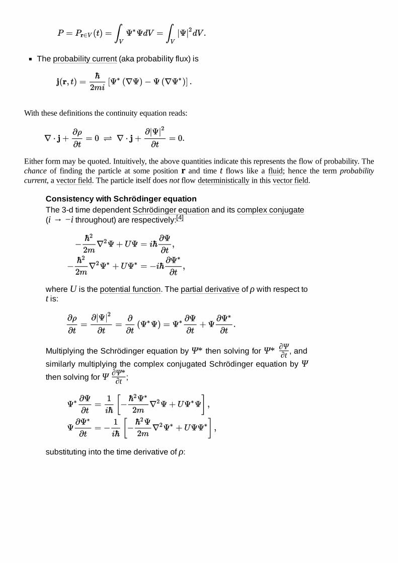
With these definitions the continuity equation reads:

Either form may be quoted. Intuitively, the above quantities indicate this represents the flow of probability. Thechance of finding the particle at some position r and time t flows like a fluid; hence the term probabilitycurrent, a vector field. The particle itself does not flow deterministically in this vector field.

Consistency with Schrödinger equationThe 3-d time dependent Schrödinger equation and its complex conjugate(i → −i throughout) are respectively:[4]

where U is the potential function. The partial derivative of ρ with respect tot is:

Multiplying the Schrödinger equation by Ψ* then solving for Ψ* ∂Ψ∂t , and

similarly multiplying the complex conjugated Schrödinger equation by Ψthen solving for Ψ ∂Ψ*

∂t ;

substituting into the time derivative of ρ:

The Laplacian operators (∇2) in the above result suggest that the righthand side is the divergence of j, and the reversed order of terms imply thisis the negative of j, altogether:

so the continuity equation is:

The integral form follows as for the general equation.

The notation and tools of special relativity, especially 4-vectors and 4-gradients, offer a convenient way towrite any continuity equation.

The density of a quantity ρ and its current j can be combined into a 4-vector called a 4-current:

where c is the speed of light. The 4-divergence of this current is:

where ∂μ is the 4-gradient and μ is an index labelling the spacetime dimension. Then the continuity equationis:

Relativistic version

Special relativity

in the usual case where there are no sources or sinks, that is, for perfectly conserved quantities like energy orcharge. This continuity equation is manifestly ("obviously") Lorentz invariant.

Examples of continuity equations often written in this form include electric charge conservation

where J is the electric 4-current; and energy-momentum conservation

where T is the stress-energy tensor.

In general relativity, where spacetime is curved, the continuity equation (in differential form) for energy,charge, or other conserved quantities involves the covariant divergence instead of the ordinary divergence.

For example, the stress–energy tensor is a second-order tensor field containing energy–momentum densities,energy–momentum fluxes, and shear stresses, of a mass-energy distribution. The differential form of energy-momentum conservation in general relativity states that the covariant divergence of the stress-energy tensor iszero:

This is an important constraint on the form the Einstein field equations take in general relativity.[5]

However, the ordinary divergence of the stress-energy tensor does not necessarily vanish:[6]

The right-hand side strictly vanishes for a flat geometry only.

As a consequence, the integral form of the continuity equation is difficult to define and not necessarily validfor a region within which spacetime is significantly curved (e.g. around a black hole, or across the wholeuniverse).[7]

Quarks and gluons have color charge, which is always conserved like electric charge, and there is a continuityequation for such color charge currents (explicit expressions for currents are given at gluon field strengthtensor).

There are many other quantities in particle physics which are often or always conserved: baryon number(proportional to the number of quarks minus the number of antiquarks), electron number, mu number, taunumber, isospin, and others.[8] Each of these has a corresponding continuity equation, possibly includingsource / sink terms.

General relativity

Particle physics

Noether's theorem

One reason that conservation equations frequently occur in physics is Noether's theorem. This states thatwhenever the laws of physics have a continuous symmetry, there is a continuity equation for some conservedphysical quantity. The three most famous examples are:

The laws of physics are invariant with respect to time-translation—for example, the laws ofphysics today are the same as they were yesterday. This symmetry leads to the continuityequation for conservation of energy.The laws of physics are invariant with respect to space-translation—for example, the laws ofphysics in Brazil are the same as the laws of physics in Argentina. This symmetry leads to thecontinuity equation for conservation of momentum.The laws of physics are invariant with respect to orientation—for example, floating in outerspace, there is no measurement you can do to say "which way is up"; the laws of physics arethe same regardless of how you are oriented. This symmetry leads to the continuity equation forconservation of angular momentum.

See Noether's theorem for proofs and details.

Conservation lawConservation formDissipative system

1. Pedlosky, Joseph (1987). Geophysical fluid dynamics (https://archive.org/details/geophysicalfluid00jose/page/10). Springer. pp. 10–13 (https://archive.org/details/geophysicalfluid00jose/page/10). ISBN 978-0-387-96387-7.

2. Clancy, L.J.(1975), Aerodynamics, Section 3.3, Pitman Publishing Limited, London3. Fielding, Suzanne. "The Basics of Fluid Dynamics" (https://community.dur.ac.uk/suzanne.fieldi

ng/teaching/BLT/sec1.pdf) (PDF). Durham University. Retrieved 22 December 2019.4. For this derivation see for example McMahon, D. (2006). Quantum Mechanics Demystified.

McGraw Hill. ISBN 0-07-145546-9.5. D. McMahon (2006). Relativity DeMystified. McGraw Hill (USA). ISBN 0-07-145545-0.6. C.W. Misner; K.S. Thorne; J.A. Wheeler (1973). Gravitation. W.H. Freeman & Co. ISBN 0-7167-

0344-0.7. Michael Weiss; John Baez. "Is Energy Conserved in General Relativity?" (http://math.ucr.edu/h

ome/baez/physics/Relativity/GR/energy_gr.html). Retrieved 2014-04-25.8. J.A. Wheeler; C. Misner; K.S. Thorne (1973). Gravitation. W.H. Freeman & Co. pp. 558–559.

ISBN 0-7167-0344-0.

Hydrodynamics, H. Lamb, Cambridge University Press, (2006 digitalization of 1932 6th edition)ISBN 978-0-521-45868-9Introduction to Electrodynamics (3rd Edition), D.J. Griffiths, Pearson Education Inc, 1999,ISBN 81-7758-293-3Electromagnetism (2nd edition), I.S. Grant, W.R. Phillips, Manchester Physics Series, 2008ISBN 0-471-92712-0

See also

References

Further reading

Gravitation, J.A. Wheeler, C. Misner, K.S. Thorne, W.H. Freeman & Co, 1973, ISBN 0-7167-0344-0

Retrieved from "https://en.wikipedia.org/w/index.php?title=Continuity_equation&oldid=1006012007"

This page was last edited on 10 February 2021, at 15:46 (UTC).

Text is available under the Creative Commons Attribution-ShareAlike License; additional terms may apply. By using thissite, you agree to the Terms of Use and Privacy Policy. Wikipedia® is a registered trademark of the WikimediaFoundation, Inc., a non-profit organization.