QCD for LHC Physics - 1

M. E. PeskinSonora Autumn School October 2008

In these lectures, I will describe some basic principles of QCD applicable to the study of hard scattering processes at hadron colliders.

The outline of the course is as follows:

1. Basic principles; parton distribution functions; Altarelli-Parisi equations

2. Parton model for hadron-hadron collisions; jets, jet observables, and jet shapes

3. Multiparton QCD amplitudes

QCD is an SU(3) Yang-Mills gauge theory, coupled to Dirac fermions (quarks) in the 3 representation of SU(3).

This theory has two important properties:

Quark confinement: The finite-energy bound states of the theory are SU(3) singlet states: .

Asymptotic freedom: The coupling constant of the theory becomes weak as the momentum tranferred a reaction becomes large.

nf

qq , qqq , gg

basic formulae of asymptotic freedom:

the solution is:

dg

d log Q= β(g)

β(g) = −b0g3

(4π)2− b1

g5

(4π)4− · · ·

g2

4π= αs(Q) =

4π

b0 log(Q2/Λ2)− 4πb1 log log(Q2/Λ2)

b30 log2(Q2/Λ2)

+ · · ·

b0 = 11− 23nf b1 = 102− 38

3nf

Bethke

PDG 2008αs(MS)(mZ) = 0.1176± 0.002

Begin our discussion with the the simplest QCD process:

I will ignore the quark masses. Then this process is very easily analyzed in terms of scattering amplitudes between states of definite helicity.

First consider with the related pure QED process

e+e− → qq

e+e− → µ+µ−

The amplitudes for between states of definite helicity are very simple:

that is,

iM(e−L

e+R→ µ−

Lµ+

R) = iM(e−

Re+L→ µ−

Rµ+

L) = ie2(1 + cos θ)

iM(e−L

e+R→ µ−

Rµ+

L) = iM(e−

Re+L→ µ−

Lµ+

R) = ie2(1 − cos θ) (1)

e+e−

→ µ+µ−

p1

p2

k1

k2

iM(e−Le+R → µ+µ−)

= 2ie2 u

s= ie2(1 + cos θ)

These formulae lead to the regularities:

with . The second formula sets the size of cross sections for all QED and electroweak processes.

dσ

d cos θ∼ (1 + cos2 θ)

σ =4πα2

3s=

87. fb

(ECM TeV)2

s = q2 = (ECM )2

SLD

e e + _ + _Z

0

For , we multiply by the quark charges and sum over colors in the final state. Then,

σ(e+e− → qq) =4πα3

3s

∑

f

3Q2f

σ(e+e− → hadrons)σ(e+e− → µ+µ−)

=∑

f

3Q2

e+e− → qq

PDG compilation

SLD

e e + _ _

Z0 q q

SLD

It is more complex to describe processes with proton initial states. Here we must treat the proton wavefunction non-perturbatively.

It is too hard a problem to solve for the structure of the proton. We need an experimental setting in which we can measure it.

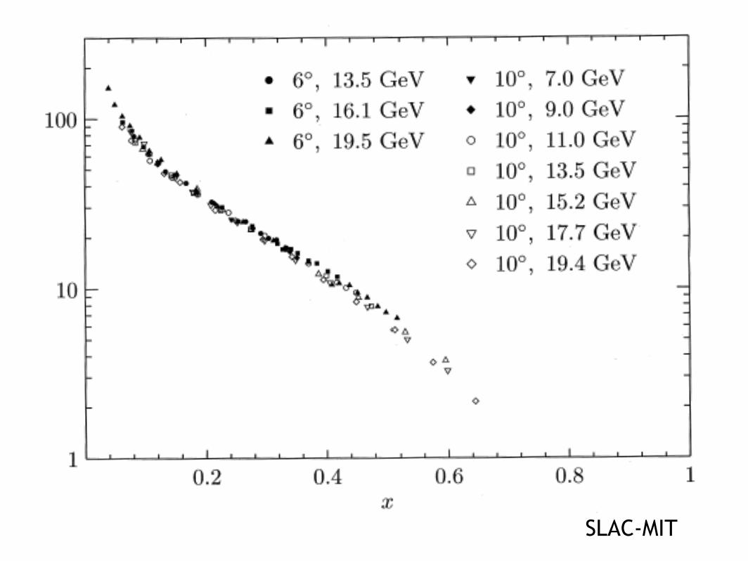
This is provided by the process deep inelastic electron scattering from protons, measured in the famous SLAC-MIT experiment.

e

p

the SLAC-MIT deep inelastic scattering experiment1967

6◦ , 7 GeV

6◦ , 16 GeV

10◦ , 17.7 GeV

SLAC-MIT

There is some wonderful kinematics, due to Feynman, that makes this process very effective for measuring the proton structure.

Work in the ep CM frame. The initial proton is coming in at high momentum. Because of asymptotic freedom, a quark in the proton cannot be at high pT with respect to the proton, except through perturbative QCD corrections. So write (ignoring all masses)

The mass of the final quark is

But this is small! so we can solve for

Then is precisely determined by the final electron momentum vector.

pµ = ξPµ 0 < ξ < 1

(p + q)2 = 2p · q + q2 = 2ξP · q −Q2

ξ =Q2

2P · Q≡ x

e

q

p+qP

p

ξ

We can now represent the proton structure by giving the probability that we find a quark at a given value of .

is called the parton distribution function.

We can fold this distribution together with the electron-quark scattering process. This requires a QED matrix element, but it is just the cross of the simple one discussed previously.

For electron momentum k, define

iM(eLqL → eLqL) = 2ie2 s/tiM(eLqR → eLqR) = 2ie2 u/t

y =2P · q

2P · k=

t

s(1− y) = −u

s

ξ

dξ fq(ξ)

fq(ξ)

Then it is straightforward to derive the formula

This formula exhibits Bjorken scaling: is only a function of x and is independent of .

is a combination of contributions from the various quark flavors. We can disentangle this by looking also at cross sections from neutrino scattering, and from other probes that I will discuss tomorrow.

F2(x)Q2

F2(x)

dσ

dxdy= F2(x)

2πα2s

Q4[1 + (1− y)2] F2(x) =

∑

f

Q2fff (x)

SLAC-MIT

H1 - 920 GeV p x 27.6 GeV e-

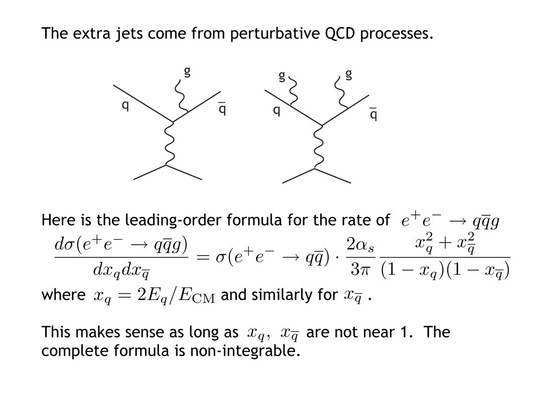
The extra jets come from perturbative QCD processes.

Here is the leading-order formula for the rate of

where and similarly for .

This makes sense as long as are not near 1. The complete formula is non-integrable.

e+e− → qqg

xq = 2Eq/ECM

xq, xq

xq

dσ(e+e− → qqg)dxqdxq

= σ(e+e− → qq) · 2αs

3π

x2q + x2

q

(1− xq)(1− xq)

The divergence comes from the fact that the virtual quark goes close to the mass shell as the gluon is emitted in the collinear direction:

In the collinear limit, the gluon emission probability is

where z is the fraction of the quark’s momentum transferred to the gluon. As or , the final state becomes difficult to distinguish from the final state without radiation.

(p + k)2 = 2p · k → 0

∫dz

43

αs

2π

∫dp2

T

p2T

1 + (1− z)2

z

z → 0 pT → 0

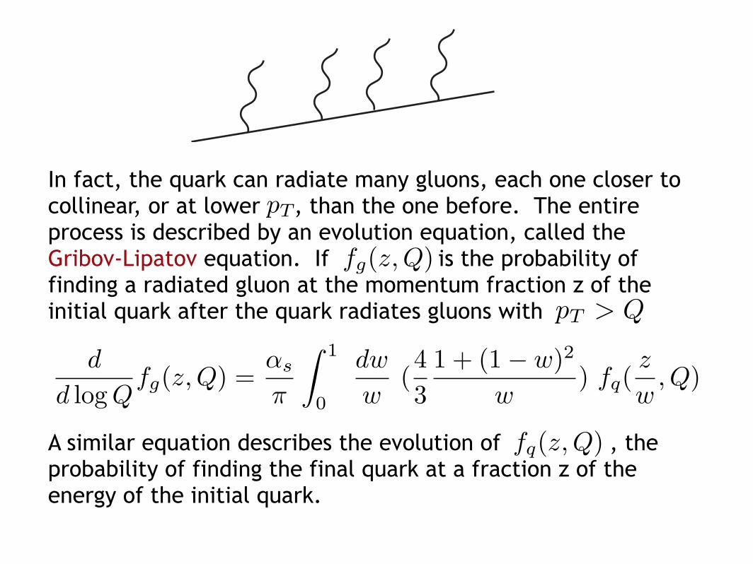
In fact, the quark can radiate many gluons, each one closer to collinear, or at lower , than the one before. The entire process is described by an evolution equation, called the Gribov-Lipatov equation. If is the probability of finding a radiated gluon at the momentum fraction z of the initial quark after the quark radiates gluons with

A similar equation describes the evolution of , the probability of finding the final quark at a fraction z of the energy of the initial quark.

pT

pT > Q

d

d log Qfg(z, Q) =

αs

π

∫ 1

0

dw

w(43

1 + (1− w)2

w) fq(

z

w, Q)

fg(z, Q)

fq(z, Q)

The general form of the evolution equation is

where i,j index quark and gluon species. The kernels are called splitting functions. So far, we have

Pg←q(z) =43

[1 + (1− z)2

z

]

Pq←q(z) =43

[1 + z2

(1− z)++

32δ(z − 1)

]

dfi(z, Q)d log Q

=αs

π

∫ 1

0

dw

w

∑

j

Pi←j(w) fj(z

w, Q)

What is the “+” in the last line?

The quark to quark splitting function has a non-integrable singularity as , associated with soft gluon radiation. However, at the same time that we add quarks at , we should subtract quarks at that have radiated. What we really want for the quark to quark splitting function, then, is a structure

whose total integral is zero.

To implement this, define the + distribution by

Using this definition, you can check that the splitting function on the previous slide satisfies

z → 1z < 1

z = 1

F (z)−Aδ(z − 1)

∫ 1

0dz

f(z)(1− z)+

=∫ 1

0dz

f(z)− f(1)(1− z)

∫ 1

0dz Pq←q(z) = 0

To describe the evolution of jets in perturbative QCD, we must consider the the additional radiation processes of gluon splitting:

Considering gluon radiation and gluon splitting, we obtain a an evolution equation with the additional kernels

This is the Altarelli-Parisi equation.

Pq←g(z) =12[z2 + (1− z)2

]

Pg←g(z) = 6[

z

(1− z)++

(1− z)z

+ z(1− z) +(1112− nf

18)δ(z − 1)

]

Quark and gluon radiation also applies to the initial-state quarks or gluons coming into a hard scattering process,

for example, deep inelastic scattering. This implies that the parton distribution functions also evolve according to the Altarelli-Parisi equations. The higher the Q to which we probe, the more quarks, antiquarks, and gluons we find in the proton structure.

filled circles - NuTeVopen squares - CCFRcrosses - CDHSW

deep-inelastic neutrino scattering

Here are the parton distribution functions generated by a recent fit to deep inelastic scattering data:

We are now set up to discuss hadron-hadron collisions. That is the subject of tomorrow’s lecture.