QSAR of heterocyclic antifungal agents by flip regressionDeeb, O., & Clare, B. (2008). QSAR of heterocyclic antifungal agents by flip regression. Journal of Computer- Aided Molecular Design, 22(12), 885-895. DOI: 10.1007/s10822-008-9223-6

Published in:Journal of Computer - Aided Molecular Design

DOI:10.1007/s10822-008-9223-6

Link to publication in the UWA Research Repository

Rights statementThe original publication is available at www.springerlink.com Post print of work supplied. Link to Publisher'swebsite supplied in Alternative Location.

General rightsCopyright owners retain the copyright for their material stored in the UWA Research Repository. The University grants no end-userrights beyond those which are provided by the Australian Copyright Act 1968. Users may make use of the material in the Repositoryproviding due attribution is given and the use is in accordance with the Copyright Act 1968.

Take down policyIf you believe this document infringes copyright, raise a complaint by contacting repository-lib@uwa.edu.au. The document will beimmediately withdrawn from public access while the complaint is being investigated.

Download date: 02. Jun. 2018

1

QSAR of heterocyclic antifungal agents by flip

regression

Omar Deeb1, Brian W. Clare2,*

1 Faculty of Pharmacy, Al-Quds University, P.O. Box 20002 Jerusalem, Palestine.

2 School of Biomedical and Chemical Sciences, The University of Western

Australia

35 Stirling Highway, Crawley, WA 6009, Australia

Tel. +61 8 64884462, Fax +61 8 64881005, email bwc@theochem.uwa.edu.au

Abstract

QSAR analysis of a set of 96 heterocyclics with antifungal activity was performed.

The results reveals that a pyridine ring is more favorable than benzene as the 6-

membered ring, for high activity, but thiazole is unfavorable as the 5-membered ring

relative to imidazole or oxazole. Methylene is the spacer leading to the highest

activity. The descriptors used are indicator variables, which account for identity of

substituent, lipophilicity and volume of substituent, and total polarizability. Unlike

previously reported results for this data set, our fits do not exceed the limitations set

by the nature of the data itself.

Keywords: QSAR, Flip regression, antifungals, AM1.

2

Introduction:

Recent decades have witnessed increasing efforts for developing new antifungal drugs

that are capable to inhibiting various diseases related to Candida albicans species, [1]

Most fungi are completely resistant to the action of antimicrobial drugs. Only a few

substances have been discovered which exert an inhibitory effect on the fungi

pathogenic for man, and most of these are relatively toxic [2]

Consequently, spurred by the need of new antifungal agents and the fact that many

effective antimicrobial drugs possess heterocyclic systems in their structure, some

novel derivatives were synthesized during the past decade [3].

Apparently, the design of new pharmacological drugs possessing novel modes of

action is required to reduce the dramatic increase in frequency of systemic infections

along with the newly appearing fungal species, the development of resistance to the

present azole therapies and also for diminishing the high toxicity of polyenes [4-6] A

wide number of known effective antimicrobial remedies include heterocyclic systems

in their structure, like imidazoles, quinazolines, benzazoles and oxazolo (4-6)

pyridines [3,6-11] although none of these substances exhibit simultaneously an

optimally desired spectrum, potency, pharmacological properties, etc.

Nowadays, the QSAR theory is extensively applied for studying the effects and

antifungal potencies of compounds [11-14] A recent QSAR study of the 96

antifungal compounds was recently reported [15] using a number of topological

descriptors. Very good R2 values, as high as 0.9370 were reported.

3

Such good correlations seem implausible, given that the data was of narrow range and

was obtained by a twofold serial dilution technique. [7-11, 16] Starting from a fixed

concentration (in mg/l) the solutions were successively tested and diluted twofold and

retested until inhibition was obtained, which was noted as the inhibitory

concentration. The concentration was then divided by the molecular weight, giving

the MIC which is the result with which we work.

Thus the inhibitory concentration is known at best to within a factor of two, which

precludes accuracy in the log inhibitory concentration data of better than ½ log 2, or

0.15 in the range of least active to most active drug, which was 1.041 in logarithmic

terms. We have simulated data using the reported logarithmic concentration plus a

uniformly distributed random error in the range ±0.15 and carried out a linear

regression of the data plus the simulated error on the data, and in 5 trials obtained a

mean R2 of 0.8866 and a mean S of 0.084, with standard deviations 0.003 and 0.002

respectively. This represents the best that can be expected in any QSAR study on this

data set, assuming no other source of error.

The results of Duchowicz et al. [15] are thus over-fitted, regardless of the statistical

techniques that were used. The present contribution is a reanalysis of this data set

using our flip regression technique [17], to allow for isostericity of the various fused

bicyclic ring systems found in the 96 compounds studied. We used variables

appropriate for a combined classical Hansch Free-Wilson approach. Indicator

variables were used for the various heterocyclic rings and for the linkers connecting

the phenyl ring to the heterocyclic system, and the lipophilicities and volumes of the

substituents on the aromatic rings, served as Hansch-type variables.

4

In continuation to our previous studies, e.g. [17-20], all in vitro inhibitory activities

against Candida albicans species are expressed as pMIC [M] = − log (MIC[M]), with

the quantity MIC(M) representing the minimum inhibitory concentration in molar

units, is modelled in this study with the descriptors mentioned above using Flip

regression technique. All in vitro inhibitory activities of 96 heterocyclics expressed as

pMIC are shown in Table 1.

A problem arises from the symmetry of the parent molecule; to deal with this

problem, we use the program FLIPSTEP, a component of the MARTHAa statistical

package, which has been described previously [17, 18].The flip regression program is

applicable to the potentially C2v-symmetric fused-ring heterocyclic. The phenyl ring,

also of C2v symmetry, bears only a 4-substituent, so we do not apply the flip

procedure to it, as the full symmetry of this ring is not broken.

The fused ring system on the other hand has its symmetry potentially broken by the

pyridine nitrogen X and the N or O atom Y. We need to consider whether or not the

location of these atoms is relevant to activity, or whether only the position of the R1

and R2 groups is relevant. Indeed it remains to be shown that even the positions of

these are significant determinants of activity.

Materials and Methods

The molecules were set up with HyperChem [21] and optimised first with one

picosecond of molecular dynamics at the molecular dynamics, and finally at the AM1

level with Mopac 6 [22] An AM1 optimization was considered adequate for these

compounds, as AM1 was developed and parameterized for common organic

5

structures such as these. Then AM1 energy calculations were carried out on the

optimized geometries using MOPAC 93 [23] software.

The lipophilicities and volumes of the substituents on the aromatic rings, calculated

by Hyperchem [21] were used as Hansch-type variables. The variables used in this

study are listed in Table 2. The descriptors in Table 2 were correlated with the

activities taken from the literature [15] for the compounds listed in Table 1 with the

programs flipstep [17], fliprand and flippred [24], which have been described

previously.

Flip regression is a technique for obtaining QSARs in molecules that have symmetry.

It was first employed by Kishida and Manabe in 1980 [25], to study the effect of

lipophilicity of substituents in some derivatives of benzenedisulfonamide. In the

context of the present problem, the molecules are heterocyclic isosteres and which

have a possible symmetry plane bisecting the 5- and 6-membered fused rings, as

shown as dashed line in Figure 1. The atom X for example may be CH or N. This may

influence activity through an electronic effect that increases or reduces the activity of

the drug, and through symmetry. if X is CH and Y NH the molecule is symmetrical

(allowing for tautomerism) and it will be immaterial whether a particular substituent

is in the R1 or R2 position. If X is N and Y is NH the two positions are isosteric, and

one of the two possible orientations may or may not be favoured over the other. The

performance of flip regression on simulated data has been described previously. [17]

Even if the molecule is not formally symmetric the asymmetry may not be reflected in

the activity data. In the absence of experimental structure information only a

calculation can indicate whether this is so.

6

For a particular case, the R1 and R2 groups may be exchanged, corresponding to

“flipping” the molecule through the symmetry plane. Where there are N different

molecules, and there are 2 possibilities for each molecule, there are 2N possible

alternative arrangements. Each of these arrangements can be analyzed in a regression

equation. Physically, the molecule will enter that arrangement on the receptor that

minimizes its binding energy. There are 2N different regression equations that must be

solved. That regression that maximizes the Fisher variance ratio, or equivalently that

maximizes R2, is chosen.

Of course, if N is at all large, this results in an extremely large number of regressions.

To render this task manageable we adopt the combinatorial optimization technique of

simulated annealing. The progress of the calculation is tracked by maintaining two N

element arrays. The first of these, the flip status starts with a value of 1 for each

element when all the substituents are arranged as they are initially set up in Table 1,

and the value is changed to –1 when that molecule is flipped.

At the conclusion of the calculation, when the flip statuses reflect the orientation of

each molecule in the best-fit position, each molecule in turn is flipped with no change

to the others, and the decrease in goodness of fit is determined. A Student’s t test

determines whether or not the change in this one compound significantly reduces the

quality of the fit, for each compound in turn. If it is not significant, this means that the

relevant compound can lay either way on the receptor. If it is significant the current

orientation is preferred. The probability value associated with the compound is stored

in the second array, the flip significance.

7

There are two consequences of this procedure that must be borne in mind. The first is

that an inflation of significance occurs. Random numbers subjected to this procedure

can give apparently highly significant regressions. The procedure cannot however

improve on an already optimal arrangement. The only way currently known to

validate the procedure is repeated randomization of the dependent variable. The

correlation coefficient for the optimal arrangement is determined. Then the dependent

variable is repeatedly randomly reassigned to the independent variable matrix, and the

correlation coefficient recalculated.

The distribution of correlation coefficients is very non-normal, but a simple

transformation, Fishers v (or z) transformation, can normalize it. The calculated

correlation coefficient from the flip regression is fixed, and has zero variance. If R is

the correlation coefficient from the randomisation trial, the quantity RRv

−+

=11ln

21 is

normally distributed, and if we have a number of R values from the randomisation

trials we can take the mean and variance of their v values and test the hypothesis that

the obtained v is greater than the mean of those generated from the randomised data.

The calculated significance level improves with the number of trials, which is an

undesirable feature. We typically carry out 5000 randomizations, and in this number

of trials we never encounter in a successful flip regression a situation where one of the

randomised v values is greater than that obtained in the actual regression. The test of v

against the mean of the randomised values to some degree quantifies this. While in

classical regression a probability value of 0.05 or less is usually regarded as

8

significant, we would tend to discount any value from the randomisation trial much

greater than approximately 10-5.

Because in this procedure the matrix of predictor variables is preserved, the influence

of colinearity is identical in both original regression and the randomisation trials. The

second point is that there are always two equivalent solutions to a problem, with flip

statuses differing by a factor of –1. Which of the two solutions is obtained in any

particular run is a matter of chance. The flip status thus has relative significance only.

The program flipstep is a backwards-stepwise variable selection procedure. It starts

with all of the initial variables in the regression, and eliminates single variables, or

flippable pairs of variables, one at a time, on the basis of colinearity with other

variables in the equation, determined by the variance inflation factor, or of the

statistical significance of the variable based on a t test. The maximum tolerated

colinearity and significance level may be set by the user. Flippable pairs of variables

must be treated as a whole, and either both are included, or both deleted.

Because a single run of simulated annealing frequently gives a non-optimal solution,

Flipstep does by default at least 5 and at most 15 independent runs and selects the best

in terms of Fisher F ratio. The selection is based on an exact equality test, rather than

equality within a tolerance, and is carried out in double precision on a 32-bit platform.

The resolution is thus approximately 1 in 1017. The fact that the equality test is usually

met many times in a given run, particularly when variable selection is nearly

complete, suggests that Flipstep is consistently finding the same, relatively small

subset of solutions out of the vast number possible.

9

Results and Discussion

The different descriptors used in this study are explained in Table 2. The

Supplementary material Table S1 summarizes the variables listed in Table 2 for the

96 compounds in Table 1.

Table 3 show the results of FLIPSTEP calculation carried out on the variables shown

in Table 2 without flipping any variables. FLIPSTEP calculations resulted in

removing I(CH2O), I(CH2NH), LDIG, Rπ, R1V, R2π, RV, I(Imi), I(C2H4), R2V

because they are statistically insignificant. ∆HS and Π were deleted due to colinearity.

Flip regression gives the equation:

pMIC[M] = -0.0698(8.3) R1π + 0.2303(5.1) I(Pyr) - 0.2542(3.4) I(Thi) + 0.3411(9.0)

I(CH2) + 0.1580(4.1) I(CH2S) + 4.015 (1)

N = 96, R2 = 0.693, S = 0.127, F = 40.60, Q2 = 0.659

Here N is the number of compounds in the regression, R2 is the square of the multiple

correlation coefficient, S is the root mean square error, F is the Fisher variance ratio

and Q2 is the R2 based on the leave-one-out technique. It should be noted that the Q2

value is Q2 from classical regression, and so does not have its usual significance. It

assumes that all flip statuses are correct, and known in advance, an assumption that is

not warranted. The numbers in parentheses are Student’s t values, with values greater

than approximately 2 indicating significance at the 0.05 probability level. The

smallest of them, that for I(Thi) corresponds to a probability value of 0.00105. Thus

10

all variables left in the equation are very highly significant. R2 is 0.693 and S 0.127,

which means that there is still some unexplained variance in the data, given that the

minimum values imposed by twofold dilution technique on the error in activity are

0.887 and 0.084 respectively.

Performing flip regression analysis while R1V is flipped with R2V and R1π is flipped

with R2π gives the equation:

pMIC[M] = 0.00078(2.7) Π - 0.00047(1.3) R1V - 0.07136(12.5) R1π + 0.00271(4.9)

R2V + 0.10119(7.9) R2π + 0.27233(8.2) I(Pyr) + 0.05504(2.4) I(Imi) – 0.22709(4.3)

I(Thi) + 0.37586(14.0) I(CH2) + 0.07112(2.7) I(CH2S) + 3.637 (2)

N = 96, R2 = 0.8772, S = 0.082, Q2 = 0.8368, F = 60.73, P = 1.6×10-38

Flipstep calculations resulted in deletion of I(CH2O), I(C2H4), I(CH2NH), Rπ, and RV

because of low significance and ∆HS because of colinearity with other descriptors.

Table 4 show FLIPSTEP results for the model suggested in equation (2). Here R1V is

obviously of very poor significance, but it must be included in the model because its

companion term R2V is of very high significance, and neither is meaningful in the

absence of the other. P is the probability value calculated by fliprand for 5000

randomizations. This value cannot be inflated by the flip procedure. This test is

similar to that recommended by Topliss et al., and because the correlation structure of

the independent variables is preserved is free from the criticism that random

independent variables are unrealistic because they are uncorrelated.

11

From the Student’s t values the most significant term is I(CH2), followed by R1π.

Note that R2 and S have now quite closely approached the limit set by the error in the

activity data. Allowing volume and lipophilicity of group R1 to swap with that of

group R2 almost completely explains the remaining variance in the data, and no

further improvement is possible. This is not to say that the other variables in Table 2

are without effect, only that any such effects cannot be determined from this particular

data set.

The results indicate that within the limits of the data set and with very high

confidence the R1 and R2 positions are opposite in their preference for lipohilic

substituents, that bulk of only one of the two is important, and that lipophilicity is

more important than volume. A pyridine ring is preferable to benzene for the 6-

membered ring with a very high degree of confidence, and imidazole or oxazole to is

preferable to thiazole for the 5-membered ring, with a lesser degree of confidence. A

methylene group is by far the preferred spacer Z. Of the indicator variables left in the

final equation only I(Pyr) correlates significantly with the flip status. This is

indicative that apart from the pyridine nitrogen there is no strong preference on the

part of the heterocyclic structure for either orientation – that is, the three 5-membered

heterocycles are truly isosteric.

Table 5 summarizes the observed activity as well as the estimated activity according

to the multilinear regression carried out on the variables in equation (2) while Fig. 2

graphically demonstrates these results.

12

Performance of FLIPSTEP

Five consecutive runs of flipstep using default settings gave apparently identical

results on the full data set, including all flip significances, but there were differences

in flip status that reflected the corresponding flip significance. As shown in Table 6

significances were exactly 1 where R1 and R2 were both H, as would be expected,

and were very close to 1 when R1 was NH2 and R2 was H, indicating little preference

of the two sites for NH2 over H.

In all other cases significances were well below 0.05, indicating quite strong

preferences for one orientation of the substituents on the isosteric ring system over the

other. The failure of the indicator variables I(Thi) and I(Imi) to correlate with flip

status is indicative that the three 5-membered rings are truly isosteric.

A validation experiment was carried out as follows: The full data set was split into a

training set and test set using the Martha routine Split, setting at 0.77 the probability

of the compound being considered going into the training set. Because of the

stochastic nature of this procedure training sets were not all of equal size. This was

done eight times. A full Flipstep run including completely independent variable

selection was carried out on each training set, and the program Flippred was then run

on the flip-optimized, variable-selected result and the corresponding test set. Flippred

does a flip regression without variable selection on the already variable-selected

training set and applies the calculated coefficients to the similarly variable-selected

test set.

13

This results in two predictions for each member of the test set, a high and a low

prediction. Because we believe that the activity of a drug reflects its energy of binding

to its receptor we assume that the high prediction is the valid one. We carried out a

univariate regression of the observed activity of the antifungal on the high-predicted

activity and we report the results in Table 7. All runs except run 7 were statistically

significant at the 0.05 level. When the results of the 8 trials are pooled the overall

significance of the difference between the original and randomised regressions comes

to 1.9×10-9. In most cases the R2 value is poor, but this is to be expected given the low

accuracy of the data, as discussed in the Introduction. Thus although the prediction

results in this data set are not sufficiently accurate to be practically useful, the overall

correlation is of very high statistical significance.

To confirm the adequacy of the settings in Flipstep for simulated annealing we carried

out 10 Flipstep runs with each of 11 cooling regimes. The starting temperature was

the same in all cases. The results are reported in Table 8. The cooling rate and number

of cycles in Flipstep are not adaptive, but are set in advance. By default we use a

cooling rate of 0.2 and 10000 cycles. Unlike most simulated annealing protocols we

are reducing the temperature by a factor of 1-C/100 every cycle, where C is the

cooling rate, rather than in constant temperature stages as is usually done. The cooling

is exponential in nature.

As may be seen from Table 8 the default regimes produces 10 out of 10 runs with R2

of 0.8772, and can be varied quite widely without affecting this. It fails

catastrophically when the rate is reduced to 0.05, but recovers completely when the

14

number of cycles is doubled. This is because under the first of these conditions the

final temperature is not low enough to stabilize the annealing.

The results deteriorate only slowly as the cooling rate is increased, giving rise to

extra, marginally poorer regression results. These results show that for this problem

our default cooling procedure is conservative, and in fact for most problems we do not

have to vary it.

When inspected, even results giving identical F and R2 results are not identical, but

differ in some flip statuses. All of the flip significance results in a sample of 10 runs

with the default cooling parameters were identical, but there were differences in the

corresponding flip statuses, rarely when the flip significance values were very small,

becoming more common when the significance became larger, deteriorating to

become completely random when the significance (i.e. probability) became 1 or

nearly 1.

A run on a Pentium 5 machine running one processor with the default settings took 56

seconds. It was estimated from runs with reduced numbers of compounds and

variables using the companion program FLIPALL, which tries all of the orientation

combinations that an exhaustive evaluation of all possible regressions for the

complete data set would take 4×1018 years for the full data set with this hardware.

The randomisation test that we carried out is essentially that recommended by Topliss

et al. Because the matrix of independent variables is preserved it is free from

objections related to changes in colinearity that apply to complete randomisation.

15

Comparison with other QSAR studies

Duchowicz et al. [15] performed regression studies on the same set of compounds

using methods such as MLR and ANN where three compounds were considered as

outliers. The highest R2 and S values they obtained are 0.94 and 0.01, respectively.

Ursu et al [26] performed principal components – stepwise regression analysis on 68

compounds and obtained R2 of 0.96 and S of 0.01. Both Ursu et al. in [26] and

Duchowicz et al in [15] have chosen their descriptors from a very large pool of

descriptors leaving much scope for chance correlations of the kind described by

Topliss et al. [27, 28]. Another drawback of these studies is that their descriptors had

no clearly understandable physical relationship to pharmacological activity.

Yalcin et al [16] performed stepwise regression analysis on a set of 61 compounds

using indicator variables, and other variables that are similar to the descriptors we

used in this study. Yalcin obtained an R2 of 0.98, S of 0.03 and Q2 of 0.67 while we

obtained R2 of 0.86, S of 0.09 and Q2 of 0.82. However, as was described above, their

results are overfitted as a result of the lack of accuracy of the data that was inherent in

the experimental technique used to obtain it.

16

However, Yalcin stated that holding a pyridine ring in the bicyclic system is important

for the heterocyclic fused system while substituting position Z with a methylene

group as a bridge element between the fused heterocyclic ring system and phenyl ring

in this set of molecules providing two fold improved potency against C. albicans and

gives higher potency for the antifungal activity, which is in agreement with our

results. Yalcin et al [16] found that having a nitro group at position R2 in the bicyclic

nucleus while position R1 was found more significant than the positions R and R2 for

the screened antifungal activity while we found that both positions are immaterial to

the presence of the nitro group.

Conclusion

We have accounted for as much of the variance in the data set as is possible within the

limits set by the experimental error, by assuming that there is no systematic global

preference for either of the two possible orientations of the fused ring system.

However, except for NH2 over H, there was highly significant preference for the

individual R1 versus R2 positions for all substituents. A pyridine ring is more

favourable than benzene as the 6-membered ring, for high activity, but thiazole is

unfavourable as the 5-membered ring relative to imidazole or oxazole. Methylene is

the spacer W leading to the highest activity.

We have used indicator variables, which account for identity of substituent without

any assumptions about the physical origin of their effect, and the simple Hansch-type

variables lipophilicity and volume of substituent. Duchowicz et al. [15] employed

topological indices selected from a very large pool, leaving much scope for chance

correlations of the kind described by Topliss et al. [27, 28], and not having clearly

17

understandable physical relationship to pharmacological activity. Unlike previously

reported results for this data set our fits do not exceed the limitations set by the nature

of the data itself.

A test of the predictive ability of our equations, was achieved as in previous studies

[24], with a high level of statistical significance. The relatively low accuracy of the

present data set precludes such a test here having practical utility.

Note:

aClare, B.W. (2008) Martha.zip, available free of charge from the site:

http://mirrors.uwa.edu.au/mirrors/weboffice/martha/

References:

1. St-Georgiev, V., Current Drug Targets, 1 (2000) 261.

2. Meyers, F.H., Jawetz, E.,Goldfien, A.Review of Medical Pharmacology.; Lange

Medical Pub; 1976.

3. Yalcin, I., Oren, I., Temiz, O.,Sener, E.A., Acta Biochim. Pol., 47 (2000) 481.

4. Rees, J.R., Pinner, R.W.,Hajjeh, R.A., Clin. Infect. Dis., 27 (1998) 1138.

5. Polak, A., Mycoses, 42 (1999) 355.

6. Fostel, J.M.,Lartey, P.A., Drug Discovery Today, 5 (2000) 25.

7. Tafi, A., Costi, R., Botta, M., Di Santo, R., Corelli, F., Massa, S., Ciacci, A.,

Manetti, F.,Artico, M., Journal of Medicinal Chemistry, 45 (2002) 2720.

8. Chan, J.H., Hong, J.S., Kuyper, L.F., Baccanari, D.P., Joyner, S.S., Tansik, R.L.,

Boytos, C.M.,Rudolph, S.K., Journal of Medicinal Chemistry, 38 (1995) 3608.

9. Elnima, E.I., Zubair, M.U.,Al-Badr, A.A., Antimicrob. Agents Chemother., 19

(1981) 29.

18

10. Goker, H., Kus, C., Boykin, D.W., Yildizc, S.,Altanlar, N., Bioorganic &

Medicinal Chemistry, 10 (2002) 2589–2596.

11. Yildiz-Oren, I., Yalcin, I., Aki-Sener, E.,Ucarturk, N., European Journal of

Medicinal Chemistry, 39 (2004) 291.

12. Garci´a-Domenech, R., Ri´os-Santamarina, I., Catala´ , A., Calabuig, C., del

Castillo, L.,Ga´lvez, J., THEOCHEM, 624 (2003) 97.

13. Hasegawa, K., Deushi, T., Yaegashi, O., Miyashita, Y.,Sasaki, S., European

Journal of Medicinal Chemistry, 30 (1995) 569.

14. Mghazli, S., Jaouad, A., Mansour, M., Villemin, D.,Cherqaoui, D., Chemosphere,

43 (2001)

15. Duchowicz, P.R., Vitale, M.G., Castro, E.A., Fernandez, M.,Caballero, J.,

Bioorganic & Medicinal Chemistry, 15 (2007) 2680–2689.

16. Yalcìn, I., Ören, I., Temiz, Ö.,Akì Sener, E., Acta Biochimica Polonica, 47

(2000) 481.

17. Clare, B.W., J. Comput.-Aided Mol. Des., 16 (2002) 611.

18. Clare, B.W.,Supuran, C.T., Bioorg. Med. Chem., 13 (2005) 2197.

19. Deeb, O., Alfalah, S.,Clare, B.W., Journal of Enzyme Inhibition and Medicinal

Chemistry, 22 (2006) 277.

20. Deeb, O.,Clare, B.W., Chemical Biology and Drug Design, 70 (2007) 437.

21. Hyperchem,6.0:Hypercube Inc,1115 NW 4th Street, Gainesville, Florida 32601-

4256 U.S.A

22. Stewart, J.J.P., Q.C.P.E. Bull., 10 (1990) 86.

23. MOPAC 93,Fujitsu Ltd.,Tokyo, Japan

24. Clare, B.W.,Supuran, C.T., Journal of Chemical Information and Modeling, 45

(2005) 1385.

19

25. Kishida, K.,Manabe, R., Med. J. Osaka Univ, 30 (1980) 95.

26. Ursu, O., Costescu, A.,Diudea, M.V., Croatica Chemica Acta, 79 (2006) 483.

27. Topliss, J.G.,Costello, R.J., J. Med. Chem., 15 (1972) 1066.

28. Topliss, J.G.,Edwards, R.J., J. Med. Chem., 22 (1979) 1238.

Supplementary Material:

The following supplementary material is available for this article:

Table S1. This material includes the different descriptors used in this study.

20

Captions for Figures:

Fig. 1 Structure and the symmetry of the compounds considered in this study

Fig. 2 Correlation of observed p MIC versus estimated

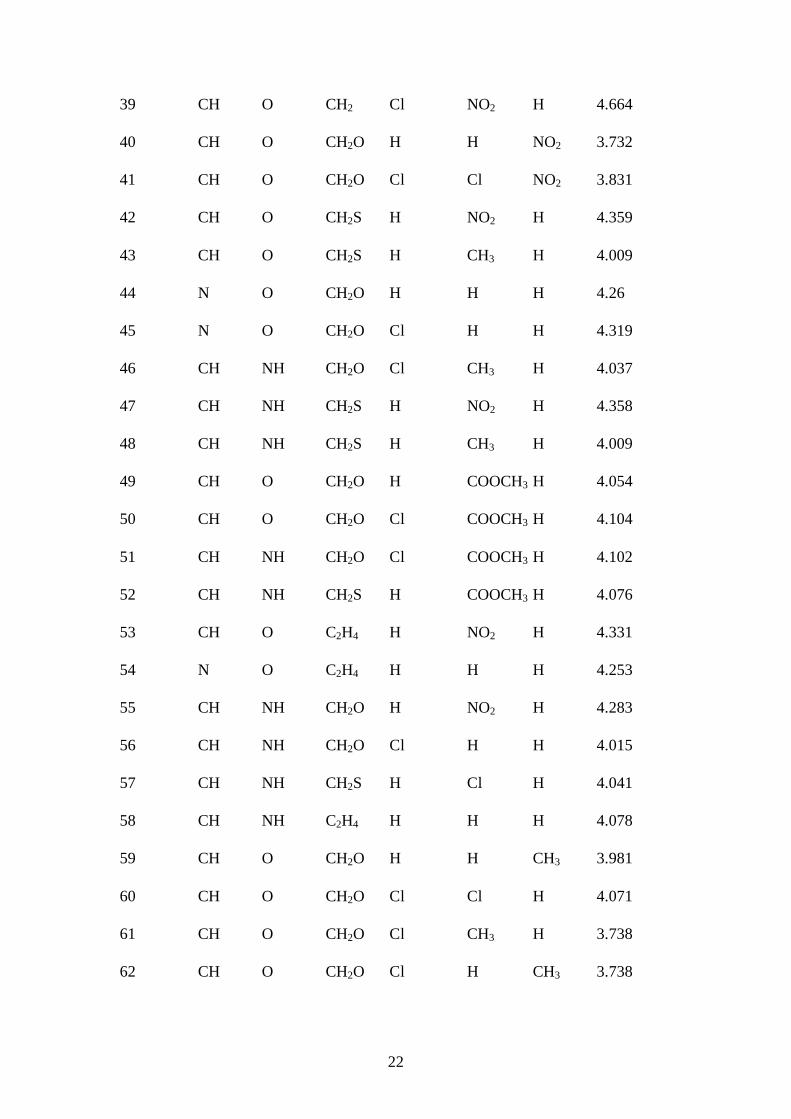
Table 1. Structure and in vitro antifungal activities against Candida Albicans.

Compound X Y Z R R1 R2 pMIC[M]

1 CH O —* H H H 3.892

2 CH O —* C(CH3)3 H H 4.001

3 CH O —* NH2 H H 3.924

4 CH O —* NHCOCH3 Cl H 4.059

5 CH O —* Cl Cl H 4.024

6 CH O —* NO2 Cl H 4.040

7 CH O —* H NO2 H 4.282

8 CH O —* CH3 NO2 H 4.308

9 CH O —* C(CH3)3 NO2 H 4.375

10 CH O —* NH2 NO2 H 4.310

11 CH O —* Cl NO2 H 4.342

12 CH O —* Br NO2 H 4.406

13 CH O —* C2H5 NH2 H 3.979

14 CH O —* F NH2 H 3.960

21

15 CH O —* N(CH3)2 NH2 H 4.005

16 CH O —* CH3 CH3 H 3.950

17 CH O —* C2H5 CH3 H 3.977

18 CH O —* OCH3 CH3 H 3.980

19 CH O —* F CH3 H 3.958

20 CH O —* NHCOCH3 CH3 H 4.027

21 CH O —* NHCH3 CH3 H 3.979

22 CH O —* N(CH3)2 CH3 H 4.004

23 N O —* CH3 H H 4.225

24 N O —* C2H5 H H 4.253

25 N O —* OCH3 H H 4.257

26 N O —* OC2H5 H H 4.283

27 N O —* NH2 H H 4.227

28 N O —* NO2 H H 4.285

29 CH O —* Br NH2 H 4.110

30 CH O CH2 OCH3 H H 4.282

31 CH O CH2 NO2 H H 4.308

32 CH O CH2 H Cl H 4.290

33 CH O CH2 OCH3 Cl H 4.340

34 CH O CH2 Br Cl H 4.410

35 CH O CH2 NO2 Cl H 4.363

36 CH O CH2 H NO2 H 4.609

37 CH O CH2 OCH3 NO2 H 4.657

38 CH O CH2 Br NO2 H 4.725

22

39 CH O CH2 Cl NO2 H 4.664

40 CH O CH2O H H NO2 3.732

41 CH O CH2O Cl Cl NO2 3.831

42 CH O CH2S H NO2 H 4.359

43 CH O CH2S H CH3 H 4.009

44 N O CH2O H H H 4.26

45 N O CH2O Cl H H 4.319

46 CH NH CH2O Cl CH3 H 4.037

47 CH NH CH2S H NO2 H 4.358

48 CH NH CH2S H CH3 H 4.009

49 CH O CH2O H COOCH3 H 4.054

50 CH O CH2O Cl COOCH3 H 4.104

51 CH NH CH2O Cl COOCH3 H 4.102

52 CH NH CH2S H COOCH3 H 4.076

53 CH O C2H4 H NO2 H 4.331

54 N O C2H4 H H H 4.253

55 CH NH CH2O H NO2 H 4.283

56 CH NH CH2O Cl H H 4.015

57 CH NH CH2S H Cl H 4.041

58 CH NH C2H4 H H H 4.078

59 CH O CH2O H H CH3 3.981

60 CH O CH2O Cl Cl H 4.071

61 CH O CH2O Cl CH3 H 3.738

62 CH O CH2O Cl H CH3 3.738

23

63 CH O CH2O H Cl H 4.344

64 CH O CH2S H H CH3 4.009

65 CH O CH2O H H H 3.955

66 CH O CH2O H NO2 H 4.034

67 CH O CH2O H Cl H 4.017

68 CH O CH2O Cl NO2 H 4.086

69 CH O CH2S H H H 4.286

70 CH O CH2S H Cl NO2 4.409

71 CH O CH2S H COOCH3 H 4.379

72 CH S CH2O H H H 3.684

73 CH S CH2O Cl H H 3.742

74 CH S CH2S H H H 4.013

75 CH NH CH2O H Cl H 4.316

76 CH NH CH2O H COOCH3 H 4.053

77 CH NH CH2O Cl Cl H 4.370

78 CH NH CH2NH H H H 3.951

79 CH NH CH2NH H CH3 H 3.977

80 CH NH C2H4 H Cl H 4.012

81 CH O —* NHCH3 H H 3.952

82 CH O —* C2H5 Cl H 4.013

83 CH O —* NHCH3 Cl H 4.025

84 CH O CH2 H H H 4.223

85 CH O CH2 Cl H H 4.290

86 CH O CH2 NO2 NO2 H 4.680

24

87 CH O CH2 Br H H 4.360

88 CH O CH2O H CH3 H 3.980

89 CH O CH2O H Cl NO2 3.785

90 CH O CH2O Cl H H 4.016

91 CH O CH2O Cl H NO2 3.785

92 CH O CH2S H H NO2 4.360

93 CH NH CH2O H H H 3.953

94 CH NH CH2O H CH3 H 3.979

95 CH NH CH2S H H H 4.284

96 CH NH C2H4 H CH3 H 4.277

• The dash “—“ indicates that there is no spacer between the two aromatic

rings.

Reprinted from Bioorg. Med. Chem. Vol. 15, by P.R. Duchowicz, M.G.

Vitale, E.A. Castro, M. Fernandez and J. Caballero, QSAR Analysis of

Heterocyclic Antifungals pages 2680-2689, copyright 2007, with permission from

Elsevier.

Table 2. Key for variables used in this study.

Variable symbol Explanation

Π The sum of Pxx, Pyy and Pzz calculated by MOPAC 6

LDIG Local dipole index: (Mean absolute difference of charge,

calculated over all bonded pairs of atoms)

∆HS Solvation energy calculated by MOPAC93, kcal

25

RV Volume of R (Å3) calculated by Hyperchem

Rπ Lipophilicity of R calculated by Hyperchem

R1V Volume of R1 (Å3) calculated by Hyperchem

R1π Lipophilicity of R1 calculated by Hyperchem

R2V Volume of R2 (Å3) calculated by Hyperchem

R2π Lipophilicity of R2 calculated by Hyperchem

I(Pyr) 1 if X is N, 0 otherwise

I(Imi) 1 if Y is NH, 0 otherwise

I(Thi) 1 if Y is S, 0 otherwise

I(CH2) 1 if Z is CH2, 0 otherwise

I(CH2O) 1 if Z is CH2O, 0 otherwise

I(CH2S) 1 if Z is CH2S, 0 otherwise

I(C2H4) 1 if Z is C2H4, 0 otherwise

I(CH2NH) 1 if Z is CH2NH, 0 otherwise

Table 3. Flipstep regression results with flipstep without flipping any variables.

Variable Coefficient t Significance VIF

Deleted

(Insignificant)

R1π -0.0698 8.27 0.00000 1.06 ICH2O) Rπ

I(Pyr) 0.23032 5.10 0.00000 1.04 I(CH2NH) R1V

I(Thi) -0.25424 3.39 0.00105 1.02 R2π RV

I(CH2) 0.3411 9.00 0.00000 1.07 I(Imi) I(C2H4)

I(CH2S) 0.15802 4.07 0.00010 1.06 R2V

26

Table 4. Flipstep regression results for flipping R1V with R2V and R1π with R2π.

Variable Coefficient t Significance VIF

Deleted

(Insignificant)

Π 0.00078 2.70 0.00844 1.83 ∆HS

R1V -0.00047 1.29 0.19990 2.20 I(C2H4)

R1π -0.07136 7.90 0.00000 1.24 RV

R2V 0.00271 4.93 0.00000 1.88 LDIG

R2π 0.10119 7.92 0.00000 1.50 Rπ

I(Pyr) 0.27233 8.15 0.00000 1.34 I(CH2NH)

I(Imi) 0.05504 2.396 0.01879 1.19 I(CH2O)

I(Thi) -0.22709 4.35 0.00004 1.17

I(CH2) 0.37586 13.98 0.00000 1.27

I(CH2S) 0.07111 2.73 0.00767 1.12

27

Table 5. Observed and estimated pMIC.

Compound pMICobserved pMICpredicted Compound pMICobserved pMICpredicted

1 3.892 3.952 49 4.054 4.066

2 4.001 4.041 50 4.104 4.035

3 3.924 3.992 51 4.102 4.091

4 4.059 4.015 52 4.076 4.182

5 4.024 3.942 53 4.331 4.264

6 4.040 3.966 54 4.253 4.235

7 4.282 4.247 55 4.283 4.311

8 4.308 4.278 56 4.015 4.055

9 4.375 4.338 57 4.041 4.088

10 4.310 4.292 58 4.078 4.034

11 4.342 4.273 59 3.981 3.927

12 4.406 4.281 60 4.071 4.168

13 3.979 4.046 61 3.738 3.960

14 3.960 4.005 62 3.738 3.947

15 4.005 4.092 63 4.344 4.148

16 3.950 3.950 64 4.009 4.045

17 3.977 3.970 65 3.955 3.959

18 3.980 3.970 66 4.034 4.251

19 3.958 3.930 67 4.017 3.921

20 4.027 4.020 68 4.086 4.270

21 3.979 3.989 69 4.286 4.075

22 4.004 4.016 70 4.409 4.545

28

23 4.225 4.246 71 4.379 4.431

24 4.253 4.266 72 3.684 3.775

25 4.257 4.266 73 3.742 3.797

26 4.283 4.290 74 4.013 3.867

27 4.227 4.257 75 4.316 4.224

28 4.285 4.264 76 4.053 4.077

29 4.110 4.052 77 4.370 4.246

30 4.282 4.362 78 3.951 4.033

31 4.308 4.363 79 3.977 3.996

32 4.290 4.286 80 4.012 3.997

33 4.340 4.327 81 3.952 4.021

34 4.410 4.313 82 4.013 3.967

35 4.363 4.328 83 4.025 3.988

36 4.609 4.617 84 4.223 4.321

37 4.657 4.659 85 4.290 4.340

38 4.725 4.645 86 4.680 4.655

39 4.664 4.638 87 4.360 4.348

40 3.732 3.774 88 3.980 3.925

41 3.831 3.753 89 3.785 3.735

42 4.359 4.283 90 4.016 3.978

43 4.009 4.028 91 3.785 3.798

44 4.260 4.294 92 4.360 4.356

45 4.319 4.243 93 3.953 4.024

46 4.037 4.023 94 3.979 3.984

47 4.358 4.347 95 4.284 4.125

29

48 4.009 4.087 96 4.277 4.247

Table 6. Flip status and significances of the 96 compounds with flipping R1V with

R2V and R1π with R2π.

Compound Flip Status Flip

Significance

Compound Flip Status Flip

Significance

1 -1 1.000 49 -1 0.013

2 -1 1.000 50 1 0.005

3 1 1.000 51 -1 0.012

4 1 0.020 52 -1 0.035

5 -1 0.012 53 -1 0.000

6 1 0.012 54 1 1.000

7 -1 0.000 55 -1 0.000

8 -1 0.000 56 1 1.000

9 -1 0.000 57 -1 0.024

10 -1 0.000 58 1 1.000

11 -1 0.000 59 -1 0.009

12 -1 0.000 60 1 0.009

13 1 0.793 61 -1 0.020

14 -1 0.795 62 1 0.019

15 1 0.804 63 1 0.012

16 -1 0.010 64 1 0.015

17 -1 0.010 65 -1 1.000

30

18 -1 0.010 66 -1 0.000

19 -1 0.010 67 -1 0.014

20 1 0.016 68 -1 0.000

21 -1 0.011 69 -1 1.000

22 -1 0.016 70 1 0.000

23 -1 1.000 71 1 0.001

24 1 1.000 72 1 1.000

25 1 1.000 73 1 1.000

26 1 1.000 74 -1 1.000

27 -1 1.000 75 1 0.012

28 -1 1.000 76 -1 0.016

29 -1 0.805 77 1 0.012

30 -1 1.000 78 1 1.000

31 1 1.000 79 -1 0.012

32 -1 0.023 80 -1 0.016

33 -1 0.021 81 1 1.000

34 -1 0.017 82 -1 0.013

35 1 0.021 83 -1 0.015

36 -1 0.000 84 -1 1.000

37 -1 0.000 85 -1 1.000

38 -1 0.000 86 -1 0.000

39 -1 0.000 87 -1 1.000

40 -1 0.000 88 1 0.010

41 -1 0.000 89 -1 0.000

31

42 -1 0.000 90 1 1.000

43 -1 0.014 91 -1 0.000

44 -1 1.000 92 1 0.000

45 -1 1.000 93 1 1.000

46 -1 0.011 94 -1 0.013

47 -1 0.000 95 -1 1.000

48 -1 0.017 96 1 0.006

Table 7 Predictions by Flippred from training sets of held-out test sets. Run R2 Prob Reg. Coef Training

set size

Variables

1 0.219 0.037 0.692 76 9

2 0.376 0.0014 0.504 72 9

3 0.450 0.0012 0.541 76 10

4 0.636 0.0057 0.412 86 9

5 0.258 0.031 0.607 78 9

6 0.157 0.050 0.223 71 7

7 0.008 0.642 0.072 69 10

8 0.177 0.045 0.444 73 12

Pooled 0.197 1.9×10-9 0.444 (601) -

32

Table 8 Effect of cooling regime on simulated annealing performance Run Cycles Cool Rate Variables F R2 Nb

1 2000 2 10

10

9

12

60.73

60.61

50.39

64.43

0.8772

0.8770

0.8793

0.8708

5

2

2

1

2 10000 9 10

10

11

60.73

60.61

52.78

0.8772

0.8770

0.8736

8

1

1

3 10000 3 10

10

10

12

60.73

60.61

59.08

50.39

0.8772

0.8770

0.8742

0.8793

5

3

1

1

4 10000 1.5 10

10

13

60.73

60.61

46.26

0.8772

0.8770

0.8800

6

3

1

5 10000 0.8 10

10

60.73

60.61

0.8772

0.8770

6

4

6 10000 0.4 10

10

12

60.73

60.61

50.39

0.8772

0.8770

0.8793

7

2

1

7 10000 0.2a 10 60.73 0.8772 10

8 10000 0.1 10 60.73 0.8772 10

9 10000 0.075 10 60.73 0.8772 10

33

10 20000 0.05 10 60.73 0.8772 10

11 10000 0.05 15

15

14

14

13

13

13

13

12

12

38.91

39.48

42.72

41.42

46.78

46.59

46.11

46.29

50.39

50.98

0.8795

0.8810

0.8807

0.8774

0.8811

0.8808

0.8797

0.8801

0.8793

0.8805

1

1

1

1

1

1

1

1

1

1

a The default b Number of apparently identical results among the 10.

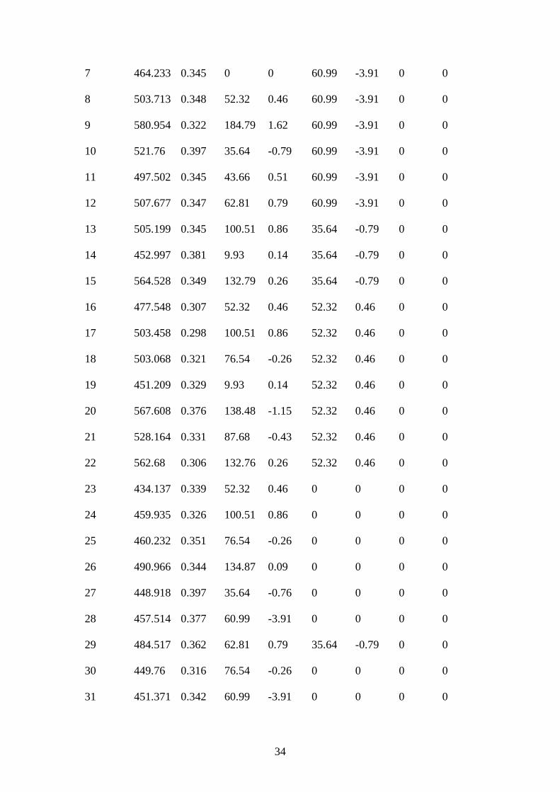
Table S1. Descriptors used in this study.

Compd. Π LdiG RV Rπ R1V R1π R2V R2π

1 406.701 0.294 0 0 0 0 0 0

2 521.248 0.285 184.79 1.62 0 0 0 0

3 457.652 0.361 35.61 -0.79 0 0 0 0

4 560.798 0.382 138.48 -1.15 43.66 0.51 0 0

5 467.03 0.294 43.66 0.51 43.66 0.51 0 0

6 498.139 0.343 60.99 -3.91 43.66 0.51 0 0

34

7 464.233 0.345 0 0 60.99 -3.91 0 0

8 503.713 0.348 52.32 0.46 60.99 -3.91 0 0

9 580.954 0.322 184.79 1.62 60.99 -3.91 0 0

10 521.76 0.397 35.64 -0.79 60.99 -3.91 0 0

11 497.502 0.345 43.66 0.51 60.99 -3.91 0 0

12 507.677 0.347 62.81 0.79 60.99 -3.91 0 0

13 505.199 0.345 100.51 0.86 35.64 -0.79 0 0

14 452.997 0.381 9.93 0.14 35.64 -0.79 0 0

15 564.528 0.349 132.79 0.26 35.64 -0.79 0 0

16 477.548 0.307 52.32 0.46 52.32 0.46 0 0

17 503.458 0.298 100.51 0.86 52.32 0.46 0 0

18 503.068 0.321 76.54 -0.26 52.32 0.46 0 0

19 451.209 0.329 9.93 0.14 52.32 0.46 0 0

20 567.608 0.376 138.48 -1.15 52.32 0.46 0 0

21 528.164 0.331 87.68 -0.43 52.32 0.46 0 0

22 562.68 0.306 132.76 0.26 52.32 0.46 0 0

23 434.137 0.339 52.32 0.46 0 0 0 0

24 459.935 0.326 100.51 0.86 0 0 0 0

25 460.232 0.351 76.54 -0.26 0 0 0 0

26 490.966 0.344 134.87 0.09 0 0 0 0

27 448.918 0.397 35.64 -0.76 0 0 0 0

28 457.514 0.377 60.99 -3.91 0 0 0 0

29 484.517 0.362 62.81 0.79 35.64 -0.79 0 0

30 449.76 0.316 76.54 -0.26 0 0 0 0

31 451.371 0.342 60.99 -3.91 0 0 0 0

35

32 425.042 0.302 0 0 43.66 0.51 0 0

33 478.112 0.319 76.54 -0.26 43.66 0.51 0 0

34 460.258 0.305 62.81 0.79 43.66 0.51 0 0

35 479.9 0.344 60.99 -3.91 43.66 0.51 0 0

36 456.824 0.345 0 0 60.99 -3.91 0 0

37 510.47 0.352 76.54 -0.26 60.99 -3.91 0 0

38 492.059 0.347 62.81 0.79 60.99 -3.91 0 0

39 482.81 0.346 43.66 0.51 60.99 -3.91 0 0

40 472.79 0.35 0 0 0 0 60.99 -3.91

41 518.898 0.34 43.66 0.51 43.66 0.51 60.99 -3.91

42 509.736 0.349 0 0 60.99 -3.91 0 0

43 486.488 0.313 0 0 52.32 0.46 0 0

44 404.971 0.343 0 0 0 0 0 0

45 429.96 0.342 43.66 0.51 0 0 0 0

46 500.42 0.334 43.66 0.51 52.32 0.46 0 0

47 522.176 0.364 0 0 60.99 -3.91 0 0

48 491.55 0.326 0 0 52.32 0.46 0 0

49 493.68 0.338 0 0 130.12 -0.5 0 0

50 545.261 0.346 43.66 0.51 130.12 -0.5 0 0

51 547.643 0.353 43.66 0.51 130.12 -0.5 0 0

52 573.371 0.352 0 0 130.12 -0.5 0 0

53 485.325 0.334 0 0 60.99 -3.91 0 0

54 420.066 0.325 0 0 0 0 0 0

55 475.64 0.366 0 0 60.99 -3.91 0 0

56 467.473 0.329 43.66 0.51 0 0 0 0

36

57 492.403 0.324 0 0 43.66 0.51 0 0

58 440.354 0.304 0 0 0 0 0 0

59 448.450 0.315 0 0 0 0 52.32 0.46

60 464.890 0.310 43.66 0.51 43.66 0.51 0 0

61 490.545 0.317 43.66 0.51 52.32 0.46 0 0

62 473.620 0.317 43.66 0.51 0 0 52.32 0.46

63 440.070 0.311 0 0 43.66 0.51 0 0

64 508.006 0.308 0 0 0 0 52.32 0.46

65 414.786 0.309 0 0 0 0 0 0

66 468.790 0.349 0 0 60.99 -3.91 0 0

67 440.070 0.311 0 0 43.66 0.51 0 0

68 493.600 0.349 43.66 0.51 60.99 -3.91 0 0

69 472.521 0.302 0 0 0 0 0 0

70 536.975 0.341 0 0 43.66 0.51 60.99 -3.91

71 542.298 0.344 0 0 130.12 -0.5 0 0

72 471.096 0.255 0 0 0 0 0 0

73 499.148 0.256 43.66 0.51 0 0 0 0

74 497.333 0.245 0 0 0 0 0 0

75 466.178 0.330 0 0 43.66 0.51 0 0

76 529.603 0.36 0 0 130.12 -0.5 0 0

77 494.23 0.329 43.66 0.51 43.66 0.51 0 0

78 439.588 0.34 0 0 0 0 0 0

79 466.29 0.342 0 0 52.22 0.46 0 0

80 466.79 0.308 0 0 43.66 0.51 0 0

81 495.102 0.33 87.68 -0.43 0 0 0 0

37

82 498.752 0.297 100.51 0.86 43.66 0.51 0 0

83 525.65 0.333 87.68 -0.43 43.66 0.51 0 0

84 397.106 0.3 0 0 0 0 0 0

85 422.625 0.302 43.66 0.51 0 0 0 0

86 505.14 0.373 60.99 -3.91 60.99 -3.91 0 0

87 431.86 0.303 62.81 0.79 0 0 0 0

88 445.99 0.315 0 0 52.32 0.46 0 0

89 496.72 0.341 0 0 43.66 0.51 60.99 -3.91

90 439.68 0.309 43.66 0.51 0 0 0 0

91 503.889 0.35 43.66 0.51 0 0 60.99 -3.91

92 512.653 0.349 0 0 0 0 60.99 -3.91

93 427.79 0.326 0 0 0 0 0 0

94 450.52 0.332 0 0 52.32 0.46 0 0

95 466.078 0.322 0 0 0 0 0 0

96 472.615 0.309 0 0 52.32 0.46 0 0

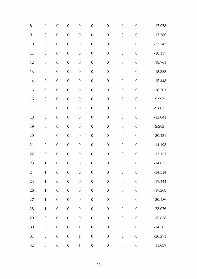
Table S1 (cont.)

Compd. I(Pyr) I(Imi) I(Thi) (ICH2) (ICH2O) (ICH2S) (IC2H4) (ICH2NH) ∆HS

1 0 0 0 0 0 0 0 0 -9.848

2 0 0 0 0 0 0 0 0 -9.804

3 0 0 0 0 0 0 0 0 -15.536

4 0 0 0 0 0 0 0 0 -19.403

5 0 0 0 0 0 0 0 0 -9.749

6 0 0 0 0 0 0 0 0 -18.327

7 0 0 0 0 0 0 0 0 -17.944

38

8 0 0 0 0 0 0 0 0 -17.978

9 0 0 0 0 0 0 0 0 -17.786

10 0 0 0 0 0 0 0 0 -23.243

11 0 0 0 0 0 0 0 0 -18.137

12 0 0 0 0 0 0 0 0 -18.761

13 0 0 0 0 0 0 0 0 -15.385

14 0 0 0 0 0 0 0 0 -15.448

15 0 0 0 0 0 0 0 0 -18.701

16 0 0 0 0 0 0 0 0 -9.993

17 0 0 0 0 0 0 0 0 -9.883

18 0 0 0 0 0 0 0 0 -12.841

19 0 0 0 0 0 0 0 0 -9.983

20 0 0 0 0 0 0 0 0 -20.451

21 0 0 0 0 0 0 0 0 -14.198

22 0 0 0 0 0 0 0 0 -13.151

23 1 0 0 0 0 0 0 0 -14.627

24 1 0 0 0 0 0 0 0 -14.514

25 1 0 0 0 0 0 0 0 -17.444

26 1 0 0 0 0 0 0 0 -17.368

27 1 0 0 0 0 0 0 0 -20.186

28 1 0 0 0 0 0 0 0 -23.076

29 0 0 0 0 0 0 0 0 -15.828

30 0 0 0 1 0 0 0 0 -14.36

31 0 0 0 1 0 0 0 0 -20.271

32 0 0 0 1 0 0 0 0 -11.057

39

33 0 0 0 1 0 0 0 0 -14.106

34 0 0 0 1 0 0 0 0 -12.008

35 0 0 0 1 0 0 0 0 -20.223

36 0 0 0 1 0 0 0 0 -19.249

37 0 0 0 1 0 0 0 0 -22.279

38 0 0 0 1 0 0 0 0 -20.381

39 0 0 0 1 0 0 0 0 -19.705

40 0 0 0 0 1 0 0 0 -21.727

41 0 0 0 0 1 0 0 0 -21.42

42 0 0 0 0 1 0 0 0 -21.898

43 0 0 0 0 0 1 0 0 -13.586

44 1 0 0 0 0 1 0 0 -18.062

45 1 0 0 0 1 0 0 0 -18.244

46 0 1 0 0 1 0 0 0 -16.884

47 0 1 0 0 1 0 0 0 -24.324

48 0 1 0 0 0 1 0 0 -16.072

49 0 0 0 0 0 1 0 0 -24.076

50 0 0 0 0 1 0 0 0 -20.641

51 0 1 0 0 1 0 0 0 -26.808

52 0 1 0 0 0 1 0 0 -23.133

53 0 0 0 0 0 0 1 0 -19.897

54 1 0 0 0 0 0 1 0 -16.423

55 0 1 0 0 1 0 0 0 -24.965

56 0 1 0 0 1 0 0 0 -16.789

57 0 1 0 0 0 1 0 0 -16.111

40

58 0 1 0 0 0 0 1 0 -16.217

59 0 0 0 0 1 0 0 0 -13.575

60 0 0 0 0 1 0 0 0 -13.588

61 0 0 0 0 1 0 0 0 -14.605

62 0 0 0 0 1 0 0 0 -13.588

63 0 0 0 0 1 0 0 0 -13.478

64 0 0 0 0 0 1 0 0 -13.898

65 0 0 0 0 1 0 0 0 -13.572

66 0 0 0 0 1 0 0 0 -21.797

67 0 0 0 0 1 0 0 0 -13.479

68 0 0 0 0 1 0 0 0 -22.149

69 0 0 0 0 0 1 0 0 -13.869

70 0 0 0 0 0 1 0 0 -21.277

71 0 0 0 0 0 1 0 0 -19.747

72 0 0 1 0 1 0 0 0 -13.876

73 0 0 1 0 1 0 0 0 -14.13

74 0 0 1 0 0 1 0 0 -13.202

75 0 1 0 0 1 0 0 0 -16.457

76 0 1 0 0 1 0 0 0 -22.73

77 0 1 0 0 1 0 0 0 -16.975

78 0 1 0 0 0 0 0 1 -17.349

79 0 1 0 0 0 0 0 1 -18.79

80 0 1 0 0 0 0 1 0 -16.397

81 0 0 0 0 0 0 0 0 -14.129

82 0 0 0 0 0 0 0 0 -9.71

41

83 0 0 0 0 0 0 0 0 -13.92

84 0 0 0 1 0 0 0 0 -11.311

85 0 0 0 1 0 0 0 0 -11.548

86 0 0 0 1 0 0 0 0 -29.181

87 0 0 0 1 0 0 0 0 -12.177

88 0 0 0 0 1 0 0 0 -13.568

89 0 0 0 0 1 0 0 0 -21.341

90 0 0 0 0 1 0 0 0 -13.588

91 0 0 0 0 1 0 0 0 -21.774

92 0 0 0 0 0 1 0 0 -21.593

93 0 1 0 0 1 0 0 0 -16.081

94 0 1 0 0 1 0 0 0 -16.763

95 0 1 0 0 0 1 0 0 -16.036

96 0 1 0 0 0 0 1 0 -16.313

42

Figure 1 Structure and symmetry of the compounds considered

43

Figure 2. Correlation of observed p MIC versus estimated.

3.8

4.0

4.2

4.4

4.6

4.8

3.8 4.0 4.2 4.4 4.6 4.8

pMIC_fit

pMIC

_obs