Date post: | 06-Apr-2018 |
Category: |
Documents |
Upload: | mansur-saburov |
View: | 218 times |
Download: | 0 times |
8/2/2019 Quadratic Stochastic Operators and Processes
http://slidepdf.com/reader/full/quadratic-stochastic-operators-and-processes 1/57
Infinite Dimensional Analysis, Quantum Probability
and Related Topics
Vol. 14, No. 2 (2011) 279–335c World Scientific Publishing Company
DOI: 10.1142/S0219025711004365
QUADRATIC STOCHASTIC OPERATORS AND PROCESSES:
RESULTS AND OPEN PROBLEMS
RASUL GANIKHODZHAEV
Department of Mechanics and Mathematics,National University of Uzbekistan,
100174, Tashkent, Uzbekistan
FARRUKH MUKHAMEDOV
Department of Computational and Theoretical Sciences Faculty of Sciences,
International Islamic University Malaysia,
P. O. Box 141, 25710, Kuantan, Pahang, Malaysia
farrukh [email protected]
UTKIR ROZIKOV
Institute of Mathematics and Information Technologies,
29, Do’rmon Yo’li str., 100125, Tashkent, Uzbekistan
Received 11 May 2009
Revised 22 November 2010Communicated by R. Rebolledo
The history of the quadratic stochastic operators can be traced back to the work of
Bernshtein (1924). For more than 80 years, this theory has been developed and many
papers were published. In recent years it has again become of interest in connection withits numerous applications in many branches of mathematics, biology and physics. But
most results of the theory were published in non-English journals, full text of which arenot accessible. In this paper we give all necessary definitions and a brief description of
the results for three cases: (i) discrete-time dynamical systems generated by quadratic
stochastic operators; (ii) continuous-time stochastic processes generated by quadraticoperators; (iii) quantum quadratic stochastic operators and processes. Moreover, we
discuss several open problems.
Keywords: Quadratic stochastic operator; quadratic stochastic process; quantumquadratic stochastic operator; quantum quadratic stochastic process; fixed point; tra-
jectory; Volterra and non-Volterra operators; ergodic; simplex.
AMS Subject Classification: 15A63, 17D92, 34A25, 35Q92, 37N25, 37L99, 46L53, 47D07,58E07, 60G07, 60G99, 60J28, 60J35, 60K35, 81P16, 81R15, 81S25
279
8/2/2019 Quadratic Stochastic Operators and Processes
http://slidepdf.com/reader/full/quadratic-stochastic-operators-and-processes 2/57
280 R. Ganikhodzhaev, F. Mukhamedov & U. Rozikov
Contents
1. Introduction 281
2. Discrete-Time Dynamical Systems Generated by QSOs 2832.1. Definitions . . . . . . . . . . . . . . . . . . . . . . . . . . . . . . . . . 283
2.2. The Volterra operators . . . . . . . . . . . . . . . . . . . . . . . . . . 283
2.3. The permuted Volterra QSO . . . . . . . . . . . . . . . . . . . . . . 287
2.4. -Volterra QSO . . . . . . . . . . . . . . . . . . . . . . . . . . . . . . 288
2.5. Non-Volterra QSO as a combination of a Volterra and non-Volterra
operators . . . . . . . . . . . . . . . . . . . . . . . . . . . . . . . . . 289
2.6. F-QSO . . . . . . . . . . . . . . . . . . . . . . . . . . . . . . . . . . . 289
2.7. Strictly non-Volterra QSO . . . . . . . . . . . . . . . . . . . . . . . . 290
2.8. Regularity of QSO . . . . . . . . . . . . . . . . . . . . . . . . . . . . 2902.9. Quadratic bistochastic operators . . . . . . . . . . . . . . . . . . . . 291
2.10. Surjective QSOs . . . . . . . . . . . . . . . . . . . . . . . . . . . . . 292
2.11. Construction of QSO. Finite case . . . . . . . . . . . . . . . . . . . . 292
2.12. Non-Volterra QSO generated by a product measure . . . . . . . . . . 293
2.13. Trajectories with historic behavior . . . . . . . . . . . . . . . . . . . 294
2.14. A generalization of Volterra QSO . . . . . . . . . . . . . . . . . . . . 294
2.15. Bernstein’s problem . . . . . . . . . . . . . . . . . . . . . . . . . . . 295
2.16. Topological conjugacy . . . . . . . . . . . . . . . . . . . . . . . . . . 295
3. Quadratic Stochastic Processes 296
3.1. Definitions . . . . . . . . . . . . . . . . . . . . . . . . . . . . . . . . . 296
3.2. E is a finite set . . . . . . . . . . . . . . . . . . . . . . . . . . . . . . 298
3.3. E is a continuum set . . . . . . . . . . . . . . . . . . . . . . . . . . . 301
3.4. Averaging of the process . . . . . . . . . . . . . . . . . . . . . . . . . 302
3.5. Simple QSPs . . . . . . . . . . . . . . . . . . . . . . . . . . . . . . . 303
3.6. Remarks . . . . . . . . . . . . . . . . . . . . . . . . . . . . . . . . . . 304
4. Quantum Quadratic Stochastic Operators 304
4.1. Quantum quadratic stochastic operators . . . . . . . . . . . . . . . . 3044.2. Quadratic operators . . . . . . . . . . . . . . . . . . . . . . . . . . . 306
4.3. Quantum quadratic stochastic operators on M2(C) . . . . . . . . . . 309
4.4. Dynamics of quadratic operators acting on S (M2(C)) . . . . . . . . . 311
4.5. On infinite-dimensional quadratic Volterra operators . . . . . . . . . 313
4.6. Construction of q.s.o. infinite case . . . . . . . . . . . . . . . . . . . 316
4.7. Remarks . . . . . . . . . . . . . . . . . . . . . . . . . . . . . . . . . . 320
5. Quantum Quadratic Stochastic Processes 320
5.1. Quantum quadratic stochastic processes . . . . . . . . . . . . . . . . 3205.2. Expansion of QQSP . . . . . . . . . . . . . . . . . . . . . . . . . . . 322
5.3. The ergodic principle . . . . . . . . . . . . . . . . . . . . . . . . . . . 324
5.4. The connection between the fiberwise Markov process
and the ergodic principle . . . . . . . . . . . . . . . . . . . . . . . . . 325
8/2/2019 Quadratic Stochastic Operators and Processes
http://slidepdf.com/reader/full/quadratic-stochastic-operators-and-processes 3/57
Quadratic Stochastic Operators 281
5.5. Marginal Markov processes . . . . . . . . . . . . . . . . . . . . . . . 326
5.6. The regularity condition . . . . . . . . . . . . . . . . . . . . . . . . . 327
5.7. Differential equations for QQSP . . . . . . . . . . . . . . . . . . . . . 328
1. Introduction
It is known that there are many systems which are described by nonlinear operators.
One of the simplest nonlinear case is quadratic one. Quadratic dynamical systems
have been proved to be a rich source of analysis for the investigation of dynamical
properties and modeling in different domains, such as population dynamics,2,10,42
physics,81,104 economy,9 mathematics.43,49,105 On the other hand, the theory of
Markov processes is a rapidly developing field with numerous applications to many
branches of mathematics and physics. However, there are physical and biologicalsystems that cannot be described by Markov processes. One of such system is given
by quadratic stochastic operators (QSO), which are related to population genet-
ics.2 The problem of studying the behavior of trajectories of quadratic stochastic
operators was stated in Ref. 105. The limit behavior and ergodic properties of
trajectories of quadratic stochastic operators and their applications to population
genetics were studied.44,48,49 In those papers a QSO arises as follows: consider a
population consisting of m species. Let x0 = (x01, . . . , x0m) be the probability dis-
tribution (where x0i = P (i) is the probability of i, i = 1, 2, . . . , m) of species in
the initial generation, and P ij,k the probability that individuals in the ith and jthspecies interbred to produce an individual k, more precisely P ij,k is the conditional
probability P (k|i, j) that ith and jth species interbred successfully, then they pro-
duce an individual k. In this paper, we consider models of free population, i.e. there
is no difference of “sex” and in any generation, the “parents” ij are independent,
i.e. P (i, j) = P (i)P ( j) = xixj . Then the probability distribution x = (x1, . . . , xm)
(the state) of the species in the first generation can be found by the total probability
xk =
m
i,j=1
P (k
|i, j)P (i, j) =
m
i,j=1
P ij,kx0i x0j , k = 1, . . . , m . (1.1)
This means that the association x0 → x defines a map V called the evolution oper-
ator . The population evolves by starting from an arbitrary state x0, then passing
to the state x = V (x) (in the next “generation”), then to the state x = V (V (x)),
and so on. Thus, states of the population described by the following discrete-time
dynamical system
x0, x = V (x), x = V 2(x), x = V 3(x), . . . (1.2)
where V n
(x) = V (V (· · · V n
(x)) · · · ) denotes the n times iteration of V to x.
8/2/2019 Quadratic Stochastic Operators and Processes
http://slidepdf.com/reader/full/quadratic-stochastic-operators-and-processes 4/57
282 R. Ganikhodzhaev, F. Mukhamedov & U. Rozikov
Note that V (defined by (1.1)) is a nonlinear (quadratic) operator, and it is
higher-dimensional if m ≥ 3. Higher-dimensional dynamical systems are important,
but there are relatively few dynamical phenomena that are currently understood.7
The main problem for a given dynamical system (1.2) is to describe the limitpoints of x(n)∞n=0 for arbitrary given x(0).
In Sec. 2 of this paper we shall discuss the recently obtained results on the
problem, and also give several open problems related to the theory of QSOs.
Note that Boltzmann considered the following problem in his paper “On the
connection between the second law of thermodynamics and probability theory in
heat equilibrium theorems”4: “calculate the probability from relations between the
numbers of different state distributions.” In the first part of Ref. 4, Boltzmann
investigated the simplest object, namely, a gas enclosed between absolutely elas-
tic walls. The molecules of the gas are absolutely elastic balls of the same radiusand mass. It is assumed that the speed of every molecule takes its values in a
certain finite set of numbers, for example, 0, 1/q, 2/q,. . . ,p/q (after any collision
the speed of any molecule can take its value only in this set). In Refs. 12, 95–97
Boltzmann’s model was studied in more general setting by introducing a continuous-
time dynamical system as a quadratic stochastic process. In Sec. 3, we shall describe
results and some open problems related to the continuous-time quadratic stochastic
processes.
However, such kind of operators and processes do not cover the case of quan-
tum systems. Therefore, in Refs. 19, 16, 58 quantum quadratic operators actingon a von Neumann algebra were defined and studied. Certain ergodic properties
of such operators were studied in Refs. 58 and 68. In these papers, dynamics of
quadratic operators were basically defined due to some recurrent rule which marks
a possibility to study asymptotic behaviors of such operators. However, with a
given quadratic operator, one can also define a nonlinear operator whose dynam-
ics (in non-commutative setting) is not studied yet. Note that in Ref. 51 another
construction of nonlinear quantum maps were suggested and some physical expla-
nations of such nonlinear quantum dynamics were discussed. There, it was also
indicated certain applications to quantum chaos. Recently, in Ref. 11 convergence
of ergodic averages associated with mentioned nonlinear operator are studied by
means of absolute contractions of von Neumann algebras. Actually, a nonlinear
dynamics of convolution operators is not investigated. Therefore, a complete anal-
ysis of dynamics of quantum quadratic operator is not well studied. In Sec. 4,
we discuss results obtained for quantum quadratic stochastic operators. On the
other hand, the defined quadratic stochastic processes in Sec. 2 do not encompass
quantum systems, therefore, it is natural to define quantum quadratic stochastic
processes (QQSP). Note that such systems also arise in the study of biological andchemical processes at the quantum level. Furthermore, in Sec. 5 we discuss and
formulate several known results for QQSO. All sections contain main definitions
which make the paper self-contained.
8/2/2019 Quadratic Stochastic Operators and Processes
http://slidepdf.com/reader/full/quadratic-stochastic-operators-and-processes 5/57
Quadratic Stochastic Operators 283
2. Discrete-Time Dynamical Systems Generated by QSOs
2.1. Definitions
The quadratic stochastic operator (QSO) is a mapping of the simplex
S m−1 =
x = (x1, . . . , xm) ∈ Rm : xi ≥ 0,
mi=1
xi = 1
(2.1)
into itself, of the form
V : xk =
mi,j=1
P ij,kxixj , k = 1, . . . , m , (2.2)
where P ij,k are coefficients of heredity and
P ij,k ≥ 0, P ij,k = P ji,k,
mk=1
P ij,k = 1, i, j, k = 1, . . . , m . (2.3)
Thus, each quadratic stochastic operator V can be uniquely defined by a cubic
matrix P = (P ij,k)ni,j,k=1 with conditions (2.3).
Note that each element x ∈ S m−1 is a probability distribution on E =
1, . . . , m.
For a given x(0) ∈ S m−1 the trajectory (orbit)
x(n), n = 0, 1, 2, . . . of x(0)
under the action of QSO (2.2) is defined by
x(n+1) = V (x(n)), where n = 0, 1, 2, . . . .
One of the main problems in mathematical biology consists in the study of the
asymptotical behavior of the trajectories. The difficulty of the problem depends on
the given matrix P. In this section we shall consider several particular cases of P
for which the above-mentioned problem is (particularly) solved.
2.2. The Volterra operators
A Volterra QSO is defined by (2.2), (2.3) and the additional assumption
P ij,k = 0, if k ∈ i, j, ∀ i,j,k ∈ E. (2.4)
The biological treatment of condition (2.4) is clear: the offspring repeats the
genotype of one of its parents.
In Ref. 28, the general form of Volterra QSO is given, i.e.
V : x = (x1, . . . , xm) ∈ S m−1 → V (x) = x = (x1, . . . , xm) ∈ S m−1.
xk = xk
1 +
mi=1
akixi
, k ∈ E, (2.5)
8/2/2019 Quadratic Stochastic Operators and Processes
http://slidepdf.com/reader/full/quadratic-stochastic-operators-and-processes 6/57
284 R. Ganikhodzhaev, F. Mukhamedov & U. Rozikov
where
aki = 2P ik,k − 1 for i = k and aii = 0, i ∈ E. (2.6)
Moreover,
aki = −aik and |aki| ≤ 1.
Denote by A = (aij)mi,j=1 the skew-symmetric matrix with entries (2.6).
Note that the operator (2.5) is a discretization of the Lotka–Volterra model47,107
which models an interacting, competing species in population. Such a model has
received considerable attention in the fields of biology, ecology, mathematics (see,
for example, Refs. 42, 43 and 103).
Let x(n)∞n=1 be the trajectory of the point x0 ∈ S m−1 under QSO (2.5). Denote
by ω(x0) the set of limit points of the trajectory. Since
x(n)
⊂S m−1 and S m−1
is compact, it follows that ω(x0) = ∅. Obviously, if ω(x0) consists of a single point,
then the trajectory converges, and ω(x0) is a fixed point of (2.5). However, looking
ahead, we remark that convergence of the trajectories is not the typical case for the
dynamical systems (2.5). Therefore, it is of particular interest to obtain an upper
bound for ω(x0), i.e. to determine a sufficiently “small” set containing ω(x0).
Denote
int S m−1 =
x ∈ S m−1 :
m
i=1
xi > 0
, ∂S m−1 = S m−1\int S m−1.
Definition 2.1. A continuous function ϕ : S m−1 → R is called a Lyapunov function
for the dynamical system (2.5) if the limit limn→∞ ϕ(x(n)) exists for any initial
point x0.
Obviously, if limn→∞ ϕ(x(n)) = c, then ω(x0) ⊂ ϕ−1(c). Consequently, for an
upper estimate of ω(x0) we should construct the set of Lyapunov functions that is
as large as possible.
Using the theory of Lyapunov functions and tournaments in Refs. 8, 25, 28–35
and 105 the theory of QSOs (2.5) was developed. DenoteP = p = ( p1, . . . , pm) ∈ S m−1 : Ap ≥ 0.
The following results are known.
Theorem 2.2. (Refs. 28 and 35) For the Volterra QSO (2.5) the following asser-
tions hold true:
(i) The set P is non-empty ;
(ii) For the dynamical system (2.5) there exists a Lyapunov function of the form
ϕ p(x) = x p1
1 · · · x pmm , where p = ( p1, . . . , pm) ∈ P, and x = (x1, . . . , xm) ∈
S m−1;
(iii) If there is r ∈ 1, . . . , m such that aij < 0 (see (2.6)) for all i ∈ 1, . . . , r,
j ∈ r + 1, . . . , m, then ϕ(x) =m
i=r+1 xi, x ∈ S m−1 is a Lyapunov function
for QSO (2.5);
8/2/2019 Quadratic Stochastic Operators and Processes
http://slidepdf.com/reader/full/quadratic-stochastic-operators-and-processes 7/57
Quadratic Stochastic Operators 285
(iv) There are Lyapunov functions of the form
ϕ(x) =xixj
, i = j, x ∈ int S m−1.
Problem 2.3. Does there exist another kind of Lyapunov function for QSO (2.5)?
The next theorem is related to the set of limit points of QSO (2.5).
Theorem 2.4. (Refs. 28 and 35) For the Volterra QSO (2.5) the following asser-
tions hold true:
(i) If x(0) ∈ int S m−1 is not a fixed point (i.e. V (x(0)) = x(0)), then ω(x0) ⊂∂S m−1.
(ii) The set ω(x0) either consists of a single point or is infinite.
(iii) If QSO (2.5) has an isolated fixed point x∗
∈ int S m−1
, then for any initial point x(0) ∈ int S m−1\x∗ the trajectory x(n) does not converge.
(iv) The “negative” trajectories V −n(x), n ≥ 0 always converge.
The formulated theorems have the following biological interpretations:
(a) The evolution begins in a neighborhood of one of the equilibrium states of the
population (stable fixed point).
(b) As a rule, the population does not tend to an equilibrium state with the passage
of time (non-stable fixed point).
(c) The “future” of the population is unstable, since certain species turn out to beon the verge of extinction with the passage of time.
(d) The “past” of such biological systems can be uniquely reproduced.
A skew-symmetric matrix A is called transversal if all even order leading (princi-
pal) minors are nonzero. A Volterra QSO V is called transversal if the corresponding
skew-symmetric matrix A is transversal.31,35,77
Problem 2.5. Define a concept of transversality for arbitrary QSO , and find nec-
essary and sufficient conditions on a matrix P = (P ij,k) of a QSO under which the
QSO is a transversal.
Note that if a Volterra QSO is transversal, then the set of fixed points X =
x ∈ S m−1 : V (x) = x, is a finite set.35
Let U ≡ U X be a neighborhood of the set X and x(n) be an arbitrary trajec-
tory. Denote
nU = | j = 1, . . . , n : x(j) ∈ U |,where |M | denotes the number of elements in M .
Then it is known thatlimn→∞
nU n
= 1,
i.e. the trajectory a large part of the time will stay in the neighborhood of the fixed
points.
8/2/2019 Quadratic Stochastic Operators and Processes
http://slidepdf.com/reader/full/quadratic-stochastic-operators-and-processes 8/57
286 R. Ganikhodzhaev, F. Mukhamedov & U. Rozikov
Denote U = U 1 ∪ U 2 ∪ · · · ∪ U t, where U i, i = 1, . . . , t is the neighborhood of the
fixed point xi.
Thus, the trajectory first visits the neighborhood of a fixed point xn1 then it
visits the neighborhood of a fixed point xn2
, and so on.
The sequence n1, n2, . . . is called the itinerary (route-march) of the trajectory
x(0), x(1), . . . . Since the set of fixed points is a finite set, the numbers n1, n2, . . . will
repeat.
Problem 2.6. Is there a trajectory with a periodic itinerary ?
On the basis of numerical calculations, Ulam105 conjectured that ergodic theo-
rem holds for any QSO V , that is, the limit limn→∞ C n(V k(x)k≥0) exists for any
x ∈ S m−1, where
C n(V k(x)k≥0) =1
n
n−1k=0
V k(x). (2.7)
In Ref. 108 Zakharevich proved that this conjecture, in general, is false. In Ref. 25
it was considered the following class of Volterra QSOs V : S 2 → S 2
x = x(1 + ay − bz),
y = y(1 − ax + cz),
z = z(1 + bx
−cy),
(2.8)
where a,b,c ∈ [−1, 1]. Note that such class contains Zakharevich’s example as a
particular case (i.e. a = b = c = 1). Note that certain extension of Zakharevich’s
example was considered in Ref. 106.
Theorem 2.7. (Ref. 25) If the parameters a,b,c for the Volterra QSO (2.8) have
the same sign and each is nonzero, then the ergodic theorem will fail for this
operator.
Problem 2.8. Find necessary and sufficient conditions on the matrix A of a
Volterra QSO under which the ergodic theorem is true on S m−1, m ≥ 2.
Note that Theorem 2.7 states that under suitable conditions, the first Cesaro
mean C n(V k(x)k≥0) of the trajectory of the Volterra QSO (2.8) does not con-
verge. But we may consider the second Cesaro mean of the first Cesaro mean, i.e.
C n(C m(V k(x)k≥0)m≥0). We are interested in the following question: does the
second Cesaro mean converge, whereas the first one diverges? If it is not so, we will
continue to consider next Cesaro means.
In Ref. 92 one of the nice properties of the Volterra QSO (2.8) has been
established.
Theorem 2.9. (Ref. 92) Let the condition of Theorem 2.7 be satisfied. Then any
order of the Cesaro mean of the trajectory of the Volterra QSO (2.8) does not
converge.
8/2/2019 Quadratic Stochastic Operators and Processes
http://slidepdf.com/reader/full/quadratic-stochastic-operators-and-processes 9/57
Quadratic Stochastic Operators 287
This theorem implies that the set of limiting points ω(x) of the trajectory
V n(x) of the Volterra QSO (2.8) has unusual structure.
Problem 2.10. Describe the set of all limiting points of the trajectory of the
Volterra QSO (2.8), whereas the condition of Theorem 2.7 is satisfied.
2.3. The permuted Volterra QSO
Let τ be a cyclic permutation on the set of indices 1, 2, . . . , m and let V be a Volterra
QSO. Define a QSO V τ by
V τ : xτ (j) = xj 1 +
m
k=1
ajkxk , j = 1, . . . , m , (2.9)
where ajk is defined in (2.6) (see Refs. 37, 35, 33 and 32).
Note that QSO V τ is a non-Volterra QSO iff τ = id.
Theorem 2.11. (Ref. 35) For any quadratic automorphism W : S m−1 → S m−1,
there exist a permutation τ and a Volterra QSO V such that W = V τ .
Corollary 2.12. The set of all quadratic automorphisms of the simplex S m−1 can
be geometrically presented as the union of m! nonintersecting cubes of dimension
m(m−1)2 .
In Refs. 75 and 89 the behavior of the trajectories of a class of non-Volterra
automorphisms of S 2 has been studied.
Problem 2.13. Investigate the asymptotic behavior of the trajectories of the oper-
ators V τ (automorphisms) for an arbitrary permutation τ .
Let us observe that any linear operator A : S m−1 → S m−1 can be considered
as a particular case of quadratic operator. Indeed, due to x∈
S m−1 we havemk=1 xk = 1, hence
Ax =
mi,j=1
a1ixixj , . . . ,
mi,j=1
amixixj
.
It is known that the k-periodic point of A is a fixed point of the linear operator
Ak. Hence, in order to find all periodic points of some linear operator, we need
to find fixed points of another linear operator. One of the nice properties of linear
operators is that a number of its isolated fixed points is at most one. Indeed, assumethat an operator A : S m−1 → S m−1 has two isolated fixed points x and y. Then for
any λ ∈ [0, 1] the point λx + (1 − λ)y is a fixed point of A, which contradicts to
assumption. Similarly, if a linear operator A has isolated k-periodic points, then the
number of its isolated k-periodic points is exactly k. However, in a quadratic case,
8/2/2019 Quadratic Stochastic Operators and Processes
http://slidepdf.com/reader/full/quadratic-stochastic-operators-and-processes 10/57
288 R. Ganikhodzhaev, F. Mukhamedov & U. Rozikov
the situation is difficult. In Refs. 8, 37 and 91 it was obtained certain estimations
to the number of periodic points of (2.9) when τ = id.
Problem 2.14. Assume τ
= id, and QSO (2.9) has an isolated k-periodic points.
Is the number of k-periodic points exactly k? In particular case, if QSO (2.9) hasan isolated fixed point , then is the number of isolated fixed points exactly one?
2.4. -Volterra QSO
Fix ∈ E and assume that elements P ij,k of the matrix P satisfy
P ij,k = 0 if k ∈ i, j for any k ∈ 1, . . . , , i, j ∈ E ; (2.10)
P ij,k > 0 for at least one pair (i, j), i
= k, j
= k if k
∈ + 1, . . . , m
.
(2.11)
Definition 2.15. (Refs. 86 and 87) For any fixed ∈ E , the QSO defined by (2.2),
(2.3), (2.10) and (2.11) is called -Volterra QSO.
Denote by V the set of all -Volterra QSOs.
Remark 2.16. Here we stress the following:
(1) The condition (2.11) guarantees that
V 1
∩ V 2 =
∅for any 1
= 2.
(2) Note that -Volterra QSO is Volterra if and only if = m.(3) By Theorem 2.4 we know that there is no periodic trajectory for Volterra QSO.
But for -Volterra QSO there are such trajectories (see Proposition 2.17 below).
Let ei = (δ1i, δ2i, . . . , δmi) ∈ S m−1, i = 1, . . . , m be the vertices of S m−1, where
δij is the Kronecker delta.
Proposition 2.17. (Refs. 86 and 87) The following assertions hold true:
(i) For any set I s =
ei1 , . . . , eis
⊂ e+1, . . . , em
, s
≤m, there exists a family
V (I s) ⊂ V such that I s is an s-cycle for every V ∈ V (I s).(ii) For any I 1, . . . , I q ⊂ + 1, . . . , m such that I i ∩ I j = ∅ (i = j,i,j = 1, . . . , q),
there exists a family V (I 1, . . . , I q) ⊂ V such that ei, i ∈ I j ( j = 1, . . . , q) is
a |I j |-cycle for every V ∈ V (I 1, . . . , I s).
Problem 2.18. Find the set of all periodic trajectories of a given -Volterra QSO.
In Refs. 75, 86 and 87 the trajectories of a class of 1-Volterra and 2-Volterra
QSOs have been investigated.
Problem 2.19. Develop the theory of dynamical systems generated by a -Volterra
QSO. Find its Lyapunov functions, the set of limit points of its trajectories etc.
Note that in Ref. 22 a quasi-Volterra QSO was considered, such an operator is
a particular case of -Volterra QSO.
8/2/2019 Quadratic Stochastic Operators and Processes
http://slidepdf.com/reader/full/quadratic-stochastic-operators-and-processes 11/57
Quadratic Stochastic Operators 289
2.5. Non-Volterra QSO as a combination of a Volterra and
non-Volterra operators
In Ref. 26 the following family of QSOs V λ : S 2 → S 2 : V λ = λV 0 + (1 − λ)V 1, 0 ≤λ ≤ 1 was considered, where V 0(x) = (x21 + 2x1x2, x22 + 2x2x3, x23 + 2x1x3) is aVolterra QSO and V 1(x) = (x21+2x2x3, x2
2+2x1x3, x23+2x1x2) is a non-Volterra one.
Note that the behavior of the trajectories of V 0 is very irregular (see Refs. 49
and 108). It has fixed points M 0 = ( 13 , 13 , 13), e1, e2, e3. The point M 0 is repelling
and ei, i = 1, 2, 3 are saddle points. These four points are also fixed points for V 1but M 0 is an attracting point for V 1. Thus, properties of V λ change depending on
the parameter λ. In Ref. 26 some examples of invariant curves and the set of limit
points of the trajectories of V λ are given.
Problem 2.20. For two arbitrary QSOs V 1 and V 2 connect the properties of V λ =λV 1 + (1 − λ)V 2, λ ∈ [0, 1] with properties of V 1 and V 2.
Problem 2.21. Describe the values of λ for which the operator V λ has n-periodic
points (n ∈ N).
2.6. F-QSO
Consider E 0 = E ∪ 0 = 0, 1, . . . , m. Fix a set F ⊂ E . This set is called the set
of “females” and the set M = E \F is called the set of “males”. The element 0 willplay the role of an “empty-body.”
We define coefficients P ij,k of the matrix P as follows:
P ij,k =
1, if k = 0, i, j ∈ F ∪ 0 or i, j ∈ M ∪ 0;
0, if k = 0, i, j ∈ F ∪ 0 or i, j ∈ M ∪ 0;
≥ 0, if i ∈ F, j ∈ M, ∀ k.
(2.12)
The biological interpretation of the coefficients (2.12) is obvious: the “child” k
can be born only if its parents are taken from different classes F and M . Generally,P ij,0 can be strictly positive for i ∈ F and j ∈ M , which corresponds, for example,
to the case in which “female” i with “male” j cannot have a “child,” because one
of them is ill or both are.
Definition 2.22. For any fixed F ⊂ E , the QSO defined by (2.2), (2.3) and (2.12)
is called the F -quadratic stochastic operator (F -QSO).
Remark 2.23. Let us note that:
(1) For any F -QSO we have P ii,0 = 1, for every i = 0, therefore such QSO is
non-Volterra.
(2) For m = 1 there is a unique F -QSO (independently of F = 1 and F = ∅)
which is constant, i.e. V (x) = (1, 0) for any x ∈ S 1.
8/2/2019 Quadratic Stochastic Operators and Processes
http://slidepdf.com/reader/full/quadratic-stochastic-operators-and-processes 12/57
290 R. Ganikhodzhaev, F. Mukhamedov & U. Rozikov
Theorem 2.24. (Ref. 88) Any F -QSO has a unique fixed point (1, 0, . . . , 0) (with
m zeros). Besides, for any x0 ∈ S m, the trajectory x(n) tends to this fixed point
exponentially rapidly.
Problem 2.25. Consider a partition ξ = E 1, . . . , E q of E, i.e. E = E 1 ∪ · · · ∪E q, E i ∩ E j = ∅, i = j. Assume P ij,k = 0 if i, j ∈ E p, for p = 1, . . . , q. Call
the corresponding operator a ξ-QSO. Is an analogue of Theorem 2.24 true for any
ξ-QSO ?
2.7. Strictly non-Volterra QSO
Recently in Ref. 89 a new class of non-Volterra QSOs have been introduced. Such
QSO is called strictly non-Volterra and is defined as follows:
P ij,k = 0 if k ∈ i, j, ∀ i,j,k ∈ E. (2.13)
One can easily check that the strictly non-Volterra operators exist only for m ≥ 3.
An arbitrary strictly non-Volterra QSO defined on S 2 (i.e. m = 3) has the form:
x = αy2 + cz2 + 2yz,
y = ax2 + dz2 + 2xz,
z = bx2 + βy2 + 2xy,
(2.14)
where
a,b,c,d,α,β ≥ 0, a + b = c + d = α + β = 1. (2.15)
Theorem 2.26. (Ref. 89) The following assertions hold true:
(i) For any values of parameters a,b,c,d,α,β with (2.15) the operator (2.14) has
a unique fixed point. Moreover , such a fixed point is not attractive.
(ii) The QSO (2.14) has 2-cycles and 3-cycles depending on the parameters (2.15).
Problem 2.27. Is Theorem 2.26 true for m ≥ 4?
2.8. Regularity of QSO
A QSO V : S m−1 → S m−1 is called regular if any of its trajectories converges to a
point a ∈ S m−1. One can see that any regular QSO has a unique fixed point, i.e. a
is that fixed point. In Ref. 40 the authors consider an arbitrary QSO V : S m−1 →S m−1 with matrix P = (P ij,k) and studied the problem of finding the smallest αmsuch that the condition P ij,k > αm implies the regularity of V .
Theorem 2.28. (Ref. 40) The following assertions hold true:
(i) If P ij,k > 12m , then V is regular.
(ii) α2 = 12 (3 − √
7).
Problem 2.29. Find exact values of αm for any m ≥ 3.
8/2/2019 Quadratic Stochastic Operators and Processes
http://slidepdf.com/reader/full/quadratic-stochastic-operators-and-processes 13/57
Quadratic Stochastic Operators 291
2.9. Quadratic bistochastic operators
Let x ∈ S m−1. Denote by x↓ the point x↓ = (x[1], . . . , x[m]) ∈ S m−1, where
x[1] ≥ · · · ≥ x[m] are the coordinates of x in non-increasing order.
If x, y ∈ S m−1 andki=1
x[i] ≤ki=1
y[i], k = 1, . . . , m ,
then we say that y majorizes x and write x ≺ y.
As is known,53 x ≺ y iff there is a doubly stochastic (bistochastic) matrix B
such that x = By. Therefore, if B is a bistochastic matrix, then Bx ≺ x for any
point x ∈ S m−1.
Reference 29 considered a more general definition.
Definition 2.30. An arbitrary continuous operator V : S m−1 → S m−1 satisfying
the condition
V (x) ≺ x, x ∈ S m−1 (2.16)
is called a bistochastic operator.
Theorem 2.31. (Refs. 29 and 41) If V : S m−1 → S m−1 is a bistochastic operator ,
then the coefficientsP ij,k
satisfy the conditions:
mi,j=1
P ij,k = m, ∀ k = 1, . . . , m; (2.17)
mj=1
P ij,k ≥ 1
2, ∀ i, k = 1, . . . , m; (2.18)
i,j∈I P ij,k ≤ t, ∀ t, k = 1, . . . , m , (2.19)
where I = i1, . . . , it is an arbitrary subset of 1, . . . , m containing t elements.
Conversely , if (2.19) holds, for a QSO , then it is a bistochastic.
Let B be the set of all bistochastic quadratic operators acting in S m−1. The set
B can be regarded as a polyhedron in an m(m2−1)2 -dimensional space. Let ExtrB
be the set of extreme points of B.
Theorem 2.32. (Refs. 36 and 29) If V ∈ ExtrB, then
P ii,k = 0 or 1;
P ij,k = 0,1
2or 1, for i = j.
Note that the converse assertion of the theorem is false.29
8/2/2019 Quadratic Stochastic Operators and Processes
http://slidepdf.com/reader/full/quadratic-stochastic-operators-and-processes 14/57
292 R. Ganikhodzhaev, F. Mukhamedov & U. Rozikov
In Ref. 4, Birkhoff characterized the set of extreme doubly stochastic matrices.
Namely his result states as follows: the set of extreme points of the set of m × m
doubly stochastic matrices coincides with the set of all permutations matrices. Sim-
ilarly, one can ask:
Problem 2.33. Describe the set of extreme points of the set of bistochastic QSO.
In Ref. 41 a subclass, called quasi-linear operators, of bistochastic QSO has been
described. Further investigations of Birkhoff’s problem for bistochastic QSO have
been studied in Ref. 38. In general, Birkhoff’s problem still remains open.
Next theorem asserts about limiting behavior of bistochastic QSO.
Theorem 2.34. (Ref. 29) Let V : S m−1
→S m−1 be a bistochastic operator , then
for any x ∈ S m−1 the Cesaro mean C n(V k(x)k≥0) converges.
Problem 2.35. Is there a regular bistochastic QSO ?
2.10. Surjective QSOs
In Refs. 23 and 54 a description of surjective QSOs defined on S m−1 for m = 2, 3, 4
and classification of extreme points of the set of such operators are given.
Problem 2.36. Describe the set of all surjective QSOs defined on S m−1 for any m ≥ 5.
2.11. Construction of QSO. Finite case
In Refs. 13 and 24 a constructive description of P (i.e. QSO) is given. The con-
struction depends on cardinality of E , namely two cases: (i) E is finite, (ii) E is
a continual set, were separately considered. Note that for the second case one of
the key problems is to determine the set of coefficients of heredity which is already
infinite-dimensional; the second problem is to investigate the quadratic operator
which corresponds to this set of coefficients. By the construction the operator V
depends on a probability measure µ being defined on a measurable space (E, F ).
Recall the construction for finite E = 1, . . . , m.
Let G = (Λ, L) be a finite graph without loops and multiple edges, where Λ is
the set of vertices and L is the set of edges of the graph.
Furthermore, let Φ be a finite set, called the set of alleles (in problems of sta-
tistical mechanics, Φ is called the range of spin). The function σ : Λ → Φ is called
a cell (in mechanics it is called configuration). Denote by Ω the set of all cells, thisset corresponds to E . Let S (Λ, Φ) be the set of all probability measures defined on
the finite set Ω.
Let Λi, i = 1, . . . , q be the set of maximal connected subgraphs (components)
of the graph G. For any M ⊂ Λ and σ ∈ Ω denote σ(M ) = σ(x) : x ∈ M . Fix two
8/2/2019 Quadratic Stochastic Operators and Processes
http://slidepdf.com/reader/full/quadratic-stochastic-operators-and-processes 15/57
Quadratic Stochastic Operators 293
cells σ1, σ2 ∈ Ω, and put
Ω(G, σ1, σ2) = σ ∈ Ω : σ(Λi) = σ1(Λi) or σ(Λi) = σ2(Λi) for all i = 1, . . . , m.
Now let µ
∈S (Λ, Φ) be a probability measure defined on Ω such that µ(σ) > 0
for any cell σ ∈ Ω; i.e. µ is a Gibbs measure with some potential.82 The hereditycoefficients P σ1σ2,σ are defined as
P σ1σ2,σ =
µ(σ)
µ(Ω(G, σ1, σ2)), if σ ∈ Ω(G, σ1, σ2),
0 otherwise.
(2.20)
Obviously, P σ1σ2,σ ≥ 0, P σ1σ2,σ = P σ2σ1,σ and
σ∈Ω P σ1σ2,σ = 1 for all σ1, σ2 ∈ Ω.
The QSO V ≡ V µ acting on the simplex S (Λ, Φ) and determined by coefficients
(2.20) is defined as follows: for an arbitrary measure λ∈
S (Λ, Φ), the measure
V (λ) = λ ∈ S (Λ, Φ) is defined by the equality
λ(σ) =
σ1,σ2∈Ω
P σ1σ2,σλ(σ1)λ(σ2) (2.21)
for any cell σ ∈ Ω.
Theorem 2.37. (Ref. 13) The QSO (2.21) is Volterra if and only if the graph G
is connected.
Thus, if Φ, G and µ are given, then we can constuct a QSO corresponding to
these objects. In Refs. 13 and 55 several examples of Φ, G and µ are consideredand the trajectories of corresponding QSOs are studied.
Note that the construction above does not give all possible QSOs. So the fol-
lowing problem is interesting.
Problem 2.38. Describe the class of QSOs which can be obtained by the
construction.
2.12. Non-Volterra QSO generated by a product measure
In Ref. 85 it was shown that if µ is the product of probability measures being defined
on each maximal connected subgraphs of G, then corresponding non-Volterra oper-
ator can be reduced to q number (where q is the number of maximal connected
subgraphs of G) of Volterra operators defined on the maximal connected subgraphs.
Let G = (Λ, L) be a finite graph and Λi, i = 1, . . . , q the set of all maximal
connected subgraphs of G. Denote by Ωi = ΦΛi the set of all configurations defined
on Λi, i = 1, . . . , q . Let µi be a probability measure defined on Ωi, such that
µi(σ) > 0 for any σ ∈ Ωi, i = 1, . . . , q .
Consider a probability measure µ on Ω = Ω1 × · · · × Ωq defined by
µ(σ) =
qi=1
µi(σi), (2.22)
where σ = (σ1, . . . , σq), with σi ∈ Ωi, i = 1, . . . , q .
8/2/2019 Quadratic Stochastic Operators and Processes
http://slidepdf.com/reader/full/quadratic-stochastic-operators-and-processes 16/57
294 R. Ganikhodzhaev, F. Mukhamedov & U. Rozikov
According to Theorem 2.37 if q = 1, then the QSO constructed on G is a Volterra
QSO.
Theorem 2.39. (Ref. 85) The QSO constructed by the construction (2.21) with
respect to measure (2.22) is reducible to q separate Volterra QSOs.
This result allows us to study a wide class of non-Volterra operators in the
framework of the well-known theory of Volterra quadratic stochastic operators.
Problem 2.40. Describe the set of all non-Volterra QSOs which are reducible to
several Volterra QSOs.
Problem 2.41. Find a measure µ different from (2.22) such that the non-Volterra
QSO corresponding to µ can be investigated in the framework of a well known theory
of QSOs.
2.13. Trajectories with historic behavior
The problem which we shall discuss here is a particular case of the problem stated
in Ref. 101.
Consider a QSO V : S m−1 → S m−1. We say that a trajectory x, V (x),
V 2(x), . . . has historic behavior if for some continuous function f : S m−1 → R
the average
limn→∞
1
n + 1
ni=0
f (V i(x))
does not exist.
If this limit does not exist, it follows that “partial averages” 1n+1
ni=0 f (V i(x))
keep changing considerably so that their values give information about the epoch
to which n belongs: they have a history.101
Problem 2.42. Find a class of QSOs such that the set of initial states which give
rise to trajectories with historic behavior has positive Lebesgue measure.
A similar problem was discussed by Ruelle in Ref. 90.
2.14. A generalization of Volterra QSO
Consider QSO (2.2), (2.3) with the additional condition
P ij,k = aikbjk , ∀ i,j,k ∈ E, (2.23)
where aik, bjk ∈ R are entries of matrices A = (aik) and B = (bjk) such thatconditions (2.3) are satisfied for the coefficients (2.23).
Then the QSO V corresponding to the coefficients (2.23) has the form
xk = (V (x))k = (A(x))k · (B(x))k, (2.24)
8/2/2019 Quadratic Stochastic Operators and Processes
http://slidepdf.com/reader/full/quadratic-stochastic-operators-and-processes 17/57
Quadratic Stochastic Operators 295
where
(A(x))k =
m
i=1
aikxi, (B(x))k =
m
j=1
bjkxj .
Note that if A (or B) is the identity matrix, then operator (2.24) is a Volterra QSO.
Problem 2.43. Develop a theory of QSOs defined by (2.24).
Note that this problem was already solved in Ref. 84. It is worth to note that in
Ref. 39 it was concerned with another generalization of Volterra QSO. It has been
established as analogies of Theorems 2.2 and 2.4.
2.15. Bernstein’s problem
The Bernstein problem49,50 is related to a fundamental statement of population
genetics, the so-called stationarity principle. This principle holds provided that the
Mendel law is assumed, but it is consistent with other mechanisms of heredity. An
adequate mathematical problem is as follows. QSO V is a Bernstein mapping if
V 2 = V . This property is just the stationarity principle. This property is known as
Hardy–Weinberg law.43 The problem is to describe all Bernstein mappings explic-
itly. The case m ≤ 2 is mathematically trivial and biologically not interesting.
Bernstein2 solved the above problem for the case m = 3 and obtained some results
for m ≥ 4. In works by Lyubich (see e.g., Refs. 49 and 50) the Bernstein problemwas solved for all m under the regularity assumption. The regularity means that
V (x) depends only on the values f (x), where f runs over all invariant linear forms.
In investigations by Lyubich,49 the algebra AV with the structure constants P ij,kplayed a very important role. Since V (x) = x2, the Bernstein property of V is
equivalent to the identity
(x2)2 = s2(x)x2.
This identity means that AV is a Bernstein algebra with respect to the algebra
homomorphism s : AV → R. The mapping V is regular iff the identity
x2y = s(x)xy
holds in the algebra AV , by definition, this identity means that AV is regular.
Problem 2.44. Describe all QSOs which satisfy V r(x) = V (x) for any x ∈ S m−1
and some r ≥ 2.
2.16. Topological conjugacy
Let V 1 : S m−1 → S m−1 and V 2 : S m−1 → S m−1 be two QSOs with coefficients P (1)ij,k
and P (2)ij,k, respectively. Recall that V 1 and V 2 are said to be topologically conjugate
if there exists a homeomorphism h : S m−1 → S m−1 such that, h V 1 = V 2 h. The
homeomorphism h is called a topological conjugacy .
8/2/2019 Quadratic Stochastic Operators and Processes
http://slidepdf.com/reader/full/quadratic-stochastic-operators-and-processes 18/57
296 R. Ganikhodzhaev, F. Mukhamedov & U. Rozikov
Mappings which are topologically conjugate are completely equivalent in terms
of their dynamics.7
Definition 2.45. A polynomial f (P ij,k) is called an indicator if from the topolog-
ically conjugateness of V 1 and V 2 it follows that
αf ≤ f (P (1)ij,k) ≤ β f and αf ≤ f (P
(2)ij,k) ≤ β f ,
where αf , β f ∈ R.
Definition 2.46. A system f 1, . . . , f t of indicators is called complete if from
αf n ≤ f n(P (1)ij,k) ≤ β f n and αf n ≤ f n(P
(2)ij,k) ≤ β f n ,
for any n = 1, . . . , t it follows the topologically conjugateness of V 1 and V 2.
A minimal complete system of indicators is called a basis.
Problem 2.47. Does there exist a finite complete system of indicators? Find the
basis of the system of indicators.
There are several approaches to solve Problem 2.47. In Ref. 77 it has been
introduced a notion of homotopic equivalence of two Volterra QSOs. A criterion of
homotopic equivalence of such kind of operators was established.
Problem 2.48. If two Volterra QSOs are homotopic equivalent , then are they topo-logically conjugate?
Note that if the last problem has a positive solution, then by means of a criterion
in Ref. 77, Problem 2.47 can be easily solved in the class of Volterra QSO.
3. Quadratic Stochastic Processes
In this section we shall describe quadratic stochastic processes, with continuous
time, which are related with quadratic operators as well as Markov process with
linear operators, this section is based on Refs. 12, 24, 76, 95–97.
3.1. Definitions
Let (E, F ) be a measurable space and let M be the set of all probability measures
on (E, F ). Let there be given a family of functions P (s,x,y,t,A) defined for
t − s ≥ 1 for all x and y ∈ E and an arbitrary measurable set A ∈ F , and assume
that the family of functions P (s,x,y,t,A) : x, y ∈ E, A ∈ F , s , t ∈ R+, t − s ≥ 1satisfies the following conditions:
(i) P (s,x,y,t,A) = P (s,y,x,t,A) for any x, y ∈ E and A ∈ F ;(ii) P (s,x,y,t, ) ∈ M for any fixed x, y ∈ E ;
(iii) P (s,x,y,t,A) as a function of x and y is measurable on (E × E, F ⊗ F ) for
any A ∈ F ;
8/2/2019 Quadratic Stochastic Operators and Processes
http://slidepdf.com/reader/full/quadratic-stochastic-operators-and-processes 19/57
Quadratic Stochastic Operators 297
(iv) (Analogue of the Chapman–Kolmogorov equation) for the initial measure µ0 ∈M and arbitrary s , τ , t ∈ R+ such that t − τ ≥ 1 and τ − s ≥ 1, we have either
(iv)A
P (s,x,y,t,A) = E
E
P (s,x,y,τ,du)P (τ,u,v,t,A)µτ (dv),
where measure µτ on (E, F ) is defined by
µτ (B) =
E
E
P (0, x , y , τ , B)µ0(dx)µ0(dy),
for any B ∈ F , or
(iv)B
P (s,x,y,t,A) = E
E
E
E
P (s,x,z,τ,du)P (s,y,v,τ,dw)
· P (τ,u,w,t,A)µs(dz)µs(dw).
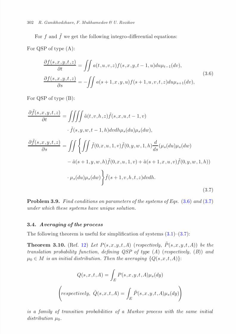
Then the process defined by the functions P (s,x,y,t,A) is called a
quadratic stochastic process (QSP) of type (A) if (iv)A holds and a
quadratic stochastic process of type (B) if (iv)B holds.
In this definition P (s,x,y,t,A) is called the transition probability which is the
probability of the following event: if x and y in E interact at time s, then oneof the elements of the set A ∈ F will be realized at time t. The realization
of interaction in physical, chemical, and biological phenomena requires some
time. We assume that the maximum of these values of time is equal to 1 (see
Boltzmann’s model4 or the biological models in Ref. 49). Hence, P (s,x,y,t,A)
is defined for t − s ≥ 1.
One can also assume the following:
(v) P (t,x,y,t + 1, A) = P (0,x,y, 1, A) for all t ≥ 1.The condition (v) can be considered as a homogeneity of the process for the
duration of time unity. From the condition it does not follow the homogeneity
of the process in general.
Thus, QSPs can be divided to three classes:
(I) homogeneous, i.e. P (s,x,y,t,A) depends only on t − s for all s and t with
t − s ≥ 1;
(II) homogeneous in duration of time unity , i.e. which satisfy the condition (v).
(III) non-homogeneous which does not belong in class (II).
In short by QSP we mean a QSP of class (II) and by P (s,x,y,t, ·) we denote
the transition probability of a QSP of type (A) and by P (s,x,y,t, ·) we denote the
transition probability of a QSP of type (B).
8/2/2019 Quadratic Stochastic Operators and Processes
http://slidepdf.com/reader/full/quadratic-stochastic-operators-and-processes 20/57
298 R. Ganikhodzhaev, F. Mukhamedov & U. Rozikov
3.2. E is a finite set
First we shall give three examples of different type of QSPs.
Example 3.1. (Ref. 97) Let E =
1, 2
and (x, 1−
x) be an initial distribution on
E , 0 ≤ x ≤ 1. Consider the following system of transition probabilities:
P [s,t]11,1 =
(1 − 2)t−s
2t−s−1[(2t−s−1 − 1)(1 − 2)sx + 1];
P [s,t]12,1 = P
[s,t]21,1 =
(1 − 2)t−s
2t−s−1
(2t−s−1 − 1)(1 − 2)sx +
1
2
;
P [s,t]22,1 =
(1 − 2)t−s
2t−s−1(2t−s−1 − 1)x;
P [s,t]ij,2 = 1 − P [s,t]ij,1 , i, j = 1, 2.
For ∈ [0, 1/2] these transition probabilities generate a QSP which is of type (A)
and type (B) simultaneously. In this case we have
x(t)1 = (1 − 2)tx, x
(t)2 = 1 − (1 − 2)tx.
For = 0 this QSP is homogeneous; for = 0 it is from class (II).
Example 3.2. (Ref. 97) Let E = 1, 2, 3 and (x1, x2, 1 − x1 − x2) be an initial
distribution on E , where x1 ≥ 0, x2 ≥ 0, x1 + x2 ≤ 1. Consider the following systemof transition probabilities:
P [s,t]11,1 = 2t−s +
2t−s−1 − 1
2t−s−1x(t+1)1 ;
P [s,t]12,1 = P
[s,t]13,1 = t−s +
2t−s−1 − 1
2t−s−1x(t+1)1 ;
P [s,t]22,1 = P
[s,t]23,1 = P
[s,t]33,1 =
2t−s−1 − 1
2t−s−1x(t+1)1 ;
P [s,t]11,2 = P
[s,t]13,2 = P
[s,t]33,2 = 2t−s−1 − 1
2t−s−1x(t+1)2 ;
P [s,t]22,2 = 2t−s +
2t−s−1 − 1
2t−s−1x(t+1)2 ;
P [s,t]12,2 = P
[s,t]23,2 = t−s +
2t−s−1 − 1
2t−s−1x(t+1)2 ;
P [s,t]ij,3 = 1 − P
[s,t]ij,1 − P
[s,t]ij,2 , i, j = 1, 2, 3,
where x(t)1 = (2)tx1, x(t)2 = (2)tx2. For ∈ [0, 1/2] these transition probabilitiesgenerate a QSP which is of type (A), but is not of type (B).
Example 3.3. (Ref. 97) Let E = 1, 2, 3 and (x1, x2, 1 − x1 − x2) be an initial
distribution on E , where x1 ≥ 0, x2 ≥ 0, x1 + x2 ≤ 1. Consider the following system
8/2/2019 Quadratic Stochastic Operators and Processes
http://slidepdf.com/reader/full/quadratic-stochastic-operators-and-processes 21/57
Quadratic Stochastic Operators 299
of transition probabilities:
P [s,t]11,1 = 2t−s +
2t−s−1 − 1
2t−s−1x(t)1 ;
P [s,t]12,1 = P
[s,t]13,1 = t−s +
2t−s−1 − 1
2t−s−1x(t)1 ;
P [s,t]22,1 = P
[s,t]23,1 = P
[s,t]33,1 =
2t−s−1 − 1
2t−s−1x(t)1 ;
P [s,t]11,2 = P
[s,t]13,2 = P
[s,t]33,2 =
2t−s−1 − 1
2t−s−1x(t)2 ;
P [s,t]22,2 = 2t−s +
2t−s−1 − 1
2t−s−1
x(t)2 ;
P [s,t]12,2 = P
[s,t]23,21 = t−s +
2t−s−1 − 1
2t−s−1x(t)2 ;
P [s,t]ij,3 = 1 − P
[s,t]ij,1 − P
[s,t]ij,2 , i, j = 1, 2, 3,
where x(t)1 = (2)tx1, x
(t)2 = (2)tx2. For ∈ [0, 1/2], these transition probabilities
generate a QSP which is of type (B), but is not of type (A).
Let E =
1, 2, . . . , n
and
x(t)1 , x
(t)2 , . . . , x
(t)n
be a distribution on E at time t.
Denote
P [s,t]ij,k = P (s,i,j,t,k).
In Refs. 95–97 by analogue of the known results of Kolmogorov46 the following
systems of differential equations are obtained:
For QSP of type (A):
∂P [s,t]ij,k
∂t =
nm,l=1
aml,k(t)x(t−1)
l P [s,t−1]
ij,k ,
∂P [s,t]ij,k
∂s= −
nm,l=1
aij,m(s + 1)x(s+1)l P
[s+1,t]ml,k ,
x(t)k =
ni,j=1
aij,k(t)x(t−1)i x
(t−1)j ,
(3.1)
where
aml,k(t) = limδ→0+0
P [t−1,t+δ]ml,k − P
[t−1,t]ml,k
δ,
the existence of the limit is assumed.
8/2/2019 Quadratic Stochastic Operators and Processes
http://slidepdf.com/reader/full/quadratic-stochastic-operators-and-processes 22/57
300 R. Ganikhodzhaev, F. Mukhamedov & U. Rozikov
For QSP of type (B):
∂ P [s,t]ij,k
∂t=
m,l,r,qalq,k(t)x(s)m x(s)r P
[s,t−1]im,l P
[s,t−1]jr,q
∂ P [s,t]ij,k
∂s=
m,l,r,q
P im,lP jr,q
d
dsx(s)m x(s)
r − (P im,lajr,q(s + 1)
+ P jr,q aim,l(s + 1))x(s)m x(s)r
P [s+1,t]lq,k .
(3.2)
Problem 3.4. Find conditions on parameters of the systems of Eqs. (3.1) and (3.2)
under which these systems have unique solution.
Here we shall describe some solutions of (3.1) for a homogeneous QSP. Thefollowing lemma is useful.
Lemma 3.5. (Ref. 76) If P [s,t]ij,k is a homogeneous QSP then for each k =
1, 2, . . . , n and any t ≥ 2 we have
x(t)k = x
(2)k .
Using Lemma 3.5 for a homogeneous QSP from Eq. (3.1) we get
∂P (t)ij,k
∂t =
n
m,l=1 aml,kx
(t−1)
l P
(t−1)
ij,m , 2 ≤ t < 3
∂P (t)ij,k
∂s=
nm,l=1
aml,kx(2)l P
(t−1)ij,m , t ≥ 3.
(3.3)
Note that in Ref. 56 the existence and uniqueness of a solution of equations
of type (3.3) is proven. But it is not clear that this solution defines a QSP. The
following calculation shows that for some boundary conditions the solution of (3.3)
defines a QSP but for some other boundary condition it does not define a QSP.
Let us consider Eq. (3.3) at n = 2 and with the following boundary condition
P (t)ij,k =
ϕ(t), if k = 1,
1 − ϕ(t), if k = 2,t ∈ [1, 2], (3.4)
where 0 ≤ ϕ(t) ≤ 1 is a continuous function.
Theorem 3.6. (Ref. 76) For n = 2 and the boundary condition (3.4), Eq. (3.3)
has the unique solution :
P (t)ij,k =
ϕ(t), if t ∈ [1, 2],ϕ(2), if t ≥ 2,
k = 1,1 − ϕ(t), if t ∈ [1, 2],
1 − ϕ(2), if t ≥ 2,k = 2.
(3.5)
8/2/2019 Quadratic Stochastic Operators and Processes
http://slidepdf.com/reader/full/quadratic-stochastic-operators-and-processes 23/57
Quadratic Stochastic Operators 301
Moreover , this solution defines a QSP if and only if ϕ(t) ≡ 1 or ϕ(t) ≡ 0 for all
t ≥ 1.
Note that any solution (with arbitrary boundary condition) of equations derived
in Ref. 46 defines a Markov process. But Theorem 3.6 shows that some solution of (3.3) (for a boundary condition) does not define a QSP.
Problem 3.7. Find all boundary conditions under which the solution of system
(3.3) defines a QSP.
3.3. E is a continuum set
We first give the following example:
Example 3.8. (Ref. 97) Let (E, F ) be a measurable space, where E is a continuum
set and let µ0 be an initial measure. Put
δx(A) =
1, if x ∈ A,
0, if x /∈ A.
Consider the following transition probability:
P (s,x,y,t,A) =1
2t−s−1 δx(A) + δy(A)
2+ (2t−s−1 − 1)µ0(A) ,
defined for t − s ≥ 1 and for all x, y ∈ E . This generates a QSP of type (A) and
(B) simultaneously.
Let E = R. Then for QSPs of type (A) and (B), one can define the following
functions of distributions:
F (s,x,y,t,z) = P (s,x,y,t,Az), F (s,x,y,t,z) = P (s,x,y,t,Az),
where Az = (−∞, z], z ∈ R. If f and f are density functions of the distributions
F and˜
F respectively, then Eqs. (iv)A and (iv)B can be written as follows: fors < τ < t such that τ − s ≥ 1 and t − τ ≥ 1,
(iv)A
f (s,x,y,t,z) =
∞−∞
f (s,x,y,τ,u)f (τ,u,v,t,z)duµτ (dv)
and
(iv)B
f (s,x,y,t,z) = ∞−∞
f (s,x,u,τ,v)f (s , y , w, τ , h)
· f (τ,v,h,t,z)dvdhµs(du)µσ(dw),
where du is the Lebesgue measure on R.
8/2/2019 Quadratic Stochastic Operators and Processes
http://slidepdf.com/reader/full/quadratic-stochastic-operators-and-processes 24/57
302 R. Ganikhodzhaev, F. Mukhamedov & U. Rozikov
For f and f we get the following integro-differential equations:
For QSP of type (A):
∂f (s,x,y,t,z)
∂t=
a(t,u,v,z)f (s,x,y,t − 1, u)duµt−1(dv),
∂f (s,x,y,t,z)
∂s= −
a(s + 1, x , y , u)f (s + 1, u, v, t , z)duµs+1(dv),
(3.6)
For QSP of type (B):
∂ f (s,x,y,t,z)
∂t = a(t,v,h,z)f (s,x,u,t − 1, v)
· f (s,y,w,t − 1, h)dvdhµs(du)µs(dw),
∂ f (s,x,y,t,z)
∂s=
f (0,x,u, 1, v)f (0, y , w, 1, h)
d
ds(µs(du)µs(dw)
− a(s + 1, y , w , h)f (0,x,u, 1, v) + a(s + 1, x , u, v)f (0, y , w, 1, h))
· µs(du)µs(dw)f (s + 1, v, h , t , z)dvdh.
(3.7)
Problem 3.9. Find conditions on parameters of the systems of Eqs. (3.6) and (3.7)
under which these systems have unique solution.
3.4. Averaging of the process
The following theorem is useful for simplification of systems (3.1)–(3.7):
Theorem 3.10. (Ref. 12) Let P (s,x,y,t,A) (respectively , P (s,x,y,t,A)) be the
translation probability function , defining QSP of type (A) (respectively , (B )) and
µ0 ∈ M is an initial distribution. Then the averaging Q(s,x,t,A):
Q(s,x,t,A) =
E
P (s,x,y,t,A)µs(dy)
respectively, Q(s,x,t,A) = E
P (s,x,y,t,A)µs(dy)is a family of transition probabilities of a Markov process with the same initial
distribution µ0.
8/2/2019 Quadratic Stochastic Operators and Processes
http://slidepdf.com/reader/full/quadratic-stochastic-operators-and-processes 25/57
Quadratic Stochastic Operators 303
Applying Theorem 3.10, Eqs. (3.1) and (3.2) can be written as
∂P [s,t]ij,k
∂t=
n
l=1
Al,k(t)P [s,t]ij,l ,
∂P [s,t]ij,k
∂s=m,l,r
Arm(s + 1)x(s+1)l P
[s+1,t]ml,k ,
x(t)k =
nm=1
Amk(t)x(t)m .
(3.8)
∂ P [s,t]ij,k
∂t
= m,l,r,q,u,v
(Aqv(t
−1)P lv,k + Alu(t
−1)P uq,k)x(s)
m x(s)r P
[s,t−1]im,l P
[s,t−1]jr,q
∂ P [s,t]ij,k
∂s= −
nl=1
(Ajl(s)P [s,t]im,l + Ail(s)P
[s,t]lj,k ),
(3.9)
where Aij(t) and Aij(t) are defined from the following equalities:
aij,k(t) =
nm=1
P ij,mAmk(t),
aij,k(t) =
nl=1
(P lj,kAil(t) + P il,kAjl(t)).
The first equations of (3.6) and (3.7) become as follows:
∂f (s,x,y,t,z)
∂t= N (t, z)f (s,x,y,t,z)
+ A(t, z)∂f (s,x,y,t,z)
∂z+ B2(t, z)
∂ 2f (s,x,y,t,z)
∂z2, (3.10)
∂ f (s,x,y,t,z)
∂s = −˜
A(s,x,z)
∂ f (s,x,y,t,z)
∂x −˜
A(s,y,z)
∂ f (s,x,y,t,z)
∂y
− B2(s,x,z)∂ 2f (s,x,y,t,z)
∂x2− B2(s,y,z)
∂ 2f (s,x,y,t,z)
∂y2.
(3.11)
Problem 3.11. Find conditions on parameters of Eqs. (3.10) and (3.11) under
which these equations have unique solution.
3.5. Simple QSPsA QSP is called simple if it has type (A) as well as type (B).
Theorem 3.12. (Ref. 97) The analytical theory of simple QSPs is analogical to
the analytical theory of Markov processes.
8/2/2019 Quadratic Stochastic Operators and Processes
http://slidepdf.com/reader/full/quadratic-stochastic-operators-and-processes 26/57
304 R. Ganikhodzhaev, F. Mukhamedov & U. Rozikov
Consider the following density function
f (s,x,y,t,z) = 2t−s−1exp(− 4t−s−1
22(t−s)−1−1(z − x+y
2t−s )2)
(22(t−s)−1
−1)π
. (3.12)
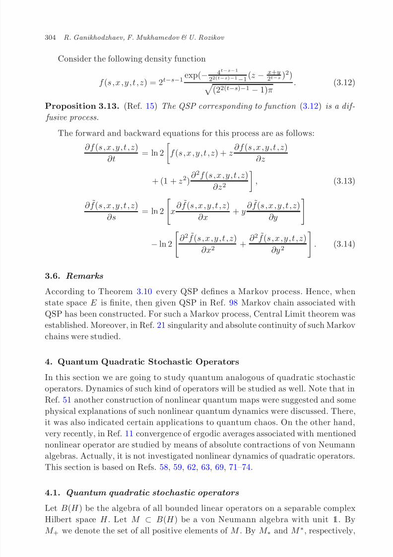
Proposition 3.13. (Ref. 15) The QSP corresponding to function (3.12) is a dif-
fusive process.
The forward and backward equations for this process are as follows:
∂f (s,x,y,t,z)
∂t= ln 2
f (s,x,y,t,z) + z
∂f (s,x,y,t,z)
∂z
+ (1 + z2)∂ 2f (s,x,y,t,z)
∂z2 , (3.13)
∂ f (s,x,y,t,z)
∂s= ln 2
x
∂ f (s,x,y,t,z)
∂x+ y
∂ f (s,x,y,t,z)
∂y
− ln 2
∂ 2f (s,x,y,t,z)
∂x2+
∂ 2f (s,x,y,t,z)
∂y2
. (3.14)
3.6. Remarks
According to Theorem 3.10 every QSP defines a Markov process. Hence, whenstate space E is finite, then given QSP in Ref. 98 Markov chain associated with
QSP has been constructed. For such a Markov process, Central Limit theorem was
established. Moreover, in Ref. 21 singularity and absolute continuity of such Markov
chains were studied.
4. Quantum Quadratic Stochastic Operators
In this section we are going to study quantum analogous of quadratic stochastic
operators. Dynamics of such kind of operators will be studied as well. Note that inRef. 51 another construction of nonlinear quantum maps were suggested and some
physical explanations of such nonlinear quantum dynamics were discussed. There,
it was also indicated certain applications to quantum chaos. On the other hand,
very recently, in Ref. 11 convergence of ergodic averages associated with mentioned
nonlinear operator are studied by means of absolute contractions of von Neumann
algebras. Actually, it is not investigated nonlinear dynamics of quadratic operators.
This section is based on Refs. 58, 59, 62, 63, 69, 71–74.
4.1. Quantum quadratic stochastic operators
Let B(H ) be the algebra of all bounded linear operators on a separable complex
Hilbert space H . Let M ⊂ B(H ) be a von Neumann algebra with unit 1. By
M + we denote the set of all positive elements of M . By M ∗ and M ∗, respectively,
8/2/2019 Quadratic Stochastic Operators and Processes
http://slidepdf.com/reader/full/quadratic-stochastic-operators-and-processes 27/57
Quadratic Stochastic Operators 305
we denote predual and dual spaces of M . The σ(M, M ∗)-topology on M is called
the ultraweak topology. By S (M ) (respectively, S 1(M )) we denote the set of all
ultraweak (respectively, norm) continuous states on M . It is well known102 that a
state is normal if and only if it is an ultraweak continuous. Now recall some notionsfrom tensor product of Banach spaces.
A linear map α : M → M is called *-morphism (respectively, a positive), if
α(x∗) = α(x)∗ for all x ∈ M (respectively, α(M +) ⊂ M +). A linear map T : M →N between von Neumann algebras M and N is said to be completely positive if
T n := T ⊗ 1Mn:Mn(M ) → Mn(N ) is positive for each n = 1, 2, . . . . It is well
known that the completely positivity can be formulated as follows: for any two
collections a1, . . . , an ∈ M and b1, . . . , bn ∈ N the following relation
ni,j=1
b∗i T (a∗i aj)bj ≥ 0. (4.1)
It is well known (cf. Ref. 80) that supn T n = T (1) for completely positive maps. It
is clear that completely positivity of T implies positivity one. In general, converse,
it is not true.
A positive (respectively, completely positive) linear map T : M → M with T 1 =
1 is called Markov operator (M.o.) (respectively, unital completely positive (ucp)
map).
Let M be a von Neumann algebra. Recall that weak (operator) closure of alge-braic tensor product M M in B(H ⊗ H ) is denoted by M ⊗ M , and it is called
tensor product of M into itself. For detail we refer the reader to Refs. 5 and 102.
By S (M ⊗ M ) we denote the set of all normal states on M ⊗ M . Let U : M ⊗M → M ⊗ M be a linear operator such that U (x ⊗ y) = y ⊗ x for all x, y ∈ M .
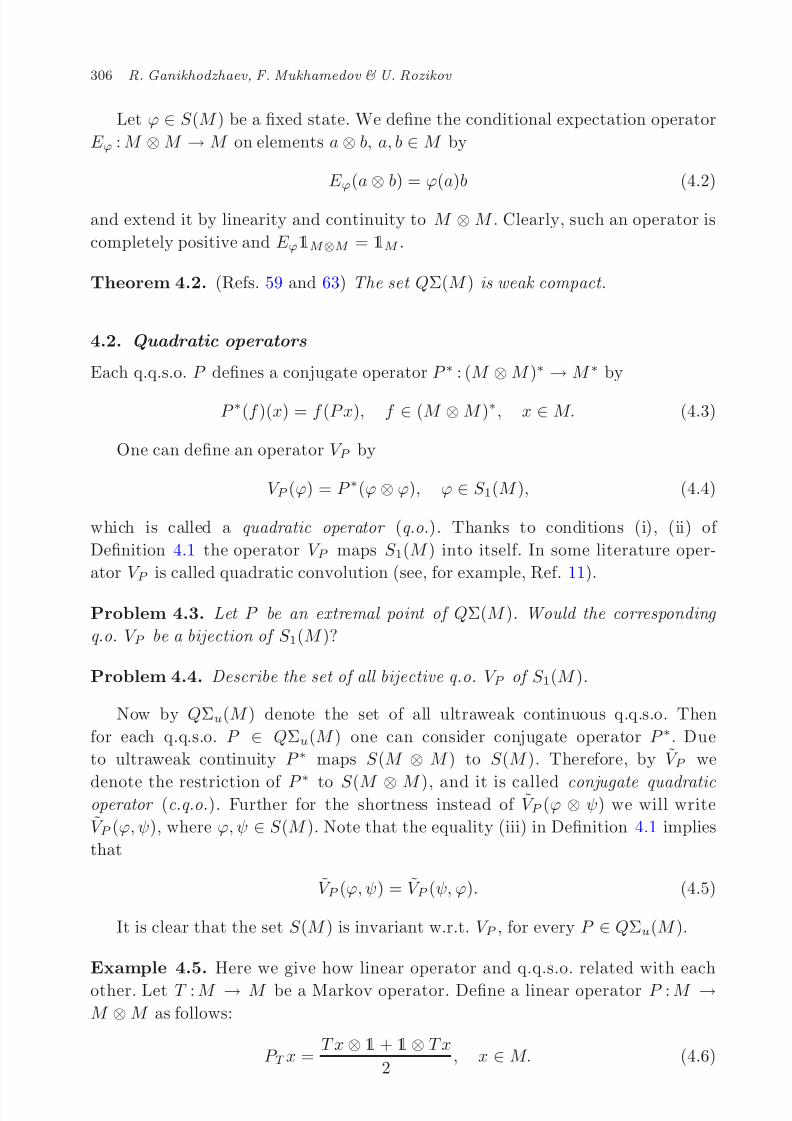
Definition 4.1. A linear operator P : M → M ⊗ M is said to be quantum quadratic
stochastic operator (q.q.s.o.) if it satisfies the following conditions:
(i) P 1M = 1M ⊗M , where 1M and 1M ⊗M are units of algebras M and M ⊗ M respectively;
(ii) P (M +) ⊂ (M ⊗ M )+;
(iii) U P x = P x for every x ∈ M .
Note that if q.q.s.o. satisfies some extra conditions (for example, coassociativity),
then such an operator generates a compact quantum group.110
By QΣ(M ) we denote the set of all q.q.s.o. on M . Let us equip these sets with
a weak topology by the following seminorms
pϕ,x(P ) = |ϕ(P x)|, ϕ ∈ M ∗ ⊗α∗0M ∗, x ∈ M,
where α∗0 is the dual norm to the smallest C ∗-crossnorm α0 on M ⊗ M (see Sec. 1.22
of Ref. 93).
8/2/2019 Quadratic Stochastic Operators and Processes
http://slidepdf.com/reader/full/quadratic-stochastic-operators-and-processes 28/57
306 R. Ganikhodzhaev, F. Mukhamedov & U. Rozikov
Let ϕ ∈ S (M ) be a fixed state. We define the conditional expectation operator
E ϕ : M ⊗ M → M on elements a ⊗ b, a, b ∈ M by
E ϕ(a
⊗b) = ϕ(a)b (4.2)
and extend it by linearity and continuity to M ⊗ M . Clearly, such an operator is
completely positive and E ϕ1M ⊗M = 1M .
Theorem 4.2. (Refs. 59 and 63) The set QΣ(M ) is weak compact.
4.2. Quadratic operators
Each q.q.s.o. P defines a conjugate operator P ∗ : (M
⊗M )∗
→M ∗ by
P ∗(f )(x) = f (P x), f ∈ (M ⊗ M )∗, x ∈ M. (4.3)
One can define an operator V P by
V P (ϕ) = P ∗(ϕ ⊗ ϕ), ϕ ∈ S 1(M ), (4.4)
which is called a quadratic operator (q.o.). Thanks to conditions (i), (ii) of
Definition 4.1 the operator V P maps S 1(M ) into itself. In some literature oper-
ator V P is called quadratic convolution (see, for example, Ref. 11).
Problem 4.3. Let P be an extremal point of QΣ(M ). Would the corresponding
q.o. V P be a bijection of S 1(M )?
Problem 4.4. Describe the set of all bijective q.o. V P of S 1(M ).
Now by QΣu(M ) denote the set of all ultraweak continuous q.q.s.o. Then
for each q.q.s.o. P ∈ QΣu(M ) one can consider conjugate operator P ∗. Due
to ultraweak continuity P ∗ maps S (M ⊗ M ) to S (M ). Therefore, by V P we
denote the restriction of P ∗
to S (M ⊗ M ), and it is called conjugate quadraticoperator (c.q.o.). Further for the shortness instead of V P (ϕ ⊗ ψ) we will write
V P (ϕ, ψ), where ϕ, ψ ∈ S (M ). Note that the equality (iii) in Definition 4.1 implies
that
V P (ϕ, ψ) = V P (ψ, ϕ). (4.5)
It is clear that the set S (M ) is invariant w.r.t. V P , for every P ∈ QΣu(M ).
Example 4.5. Here we give how linear operator and q.q.s.o. related with each
other. Let T : M → M be a Markov operator. Define a linear operator P : M →M ⊗ M as follows:
P T x =T x ⊗ 1 + 1⊗ T x
2, x ∈ M. (4.6)
8/2/2019 Quadratic Stochastic Operators and Processes
http://slidepdf.com/reader/full/quadratic-stochastic-operators-and-processes 29/57
Quadratic Stochastic Operators 307
It is clear that P T is q.q.s.o. Then associated c.q.o. and q.o. have the following form
respectively:
V P T (ϕ, ψ)(x) =1
2
(ϕ + ψ)(T x),
V P T (ϕ)(x) = ϕ(T x), x ∈ M,(4.7)
for every ϕ, ψ ∈ S (M ). Thus linear operator can be viewed as a particular case of
q.q.s.o. If T is the identity operator, then from (4.7) we can find that the associated
q.o. would also be the identity operator of S (M ).
Proposition 4.6. (Ref. 59) Each q.q.s.o. P ∈ QΣu(M ) defines a linear operator
T : M ∗ → Σ(M ) by
T (ϕ)(x) = E ϕ(P x), ϕ ∈ M ∗, x ∈ M. (4.8)Moreover , for every ϕ, ψ ∈ M ∗ holds
T ∗(ϕ)ψ = T ∗(ψ)ϕ, T (ϕ) ≤ 2ϕ1, (4.9)
where T ∗(ϕ)ψ(a) = ψ(T (ϕ)(a)). In addition ,
V P (ϕ ⊗ ψ) = T ∗(ϕ)ψ, ∀ ϕ, ψ ∈ M ∗. (4.10)
Note that a similar result can be proved for arbitrary q.q.s.o. (i.e. without
ultraweak continuity).
One can see that the trajectory ϕ(n) = V nP (ϕ) of ϕ ∈ S 1(M ) under the action
of V P can be written as follows:
ϕ(n) = T ∗(ϕ(n−1))T ∗(ϕ(n−2)) · · · T ∗(ϕ)ϕ. (4.11)
A quadratic operator V P is called Abelian if the equation T ∗(ϕ)T ∗(ψ) =
T ∗(ψ)T ∗(ϕ) holds for all ϕ, ψ ∈ S 1(M ).
For an Abelian quadratic operator using (4.11) one finds
ϕ(n) = T 2n−1∗ (ϕ)ϕ. (4.12)
In Ref. 109, the formula (4.12) allowed us to use properties of Markov operators
acting on finite-dimensional spaces and proved the following:
Theorem 4.7. (Ref. 109) Let M is a finite-dimensional von Neumann algebra ,
and V P be an Abelian quadratic operator on S 1(M ). Let ϕ(n) be the trajectory
of an arbitrary point ϕ ∈ S 1(M ) w.r.t. V P . By ω(ϕ) we denote the set of limiting
points of ϕ(n). Then
(i) ω(ϕ) = ϕ1, . . . , ϕs is a finite set ;
(ii) the sequence of means
1
n + 1
n+1k=1
ϕ(k) (4.13)
converges as n → ∞.
8/2/2019 Quadratic Stochastic Operators and Processes
http://slidepdf.com/reader/full/quadratic-stochastic-operators-and-processes 30/57
308 R. Ganikhodzhaev, F. Mukhamedov & U. Rozikov
Problem 4.8. For an Abelian quadratic operator given on arbitrary von Neumann
algebra , investigate properties of ω(ϕ) and the convergence of (4.13). Note that , in
this setting , one can consider several kinds of convergence such as weak convergence,
strong etc.
Problem 4.9. Classify all Abelian quadratic operators.
A linear map V : M ∗⊗α∗0M ∗ → M ∗ is called conjugate quadratic operator if the
following conditions hold
(i) V (S (M ⊗ M )) ⊂ S (M );
(ii) V (ϕ ⊗ ψ) = V (ψ ⊗ ϕ), ∀ ϕ, ψ ∈ M ∗.
By QΣV (M ) we denote the set of all conjugate quadratic operators.
Proposition 4.10. Every V ∈ QΣV (M ) uniquely defines a q.q.s.o. P ∈ QΣu(M ).
Let P ∈ QΣ(M ) and consider the corresponding q.o. V P on S 1(M ).
Definition 4.11. A q.o. V P is called
(i) asymptotically stable if there exists a state µ ∈ S 1(M ) such that for any ϕ ∈S 1(M ) one has
limn→∞
V nP (ϕ) − µ1 = 0, (4.14)
where by · 1 we denote the norm on M ∗;(ii) weak asymptotically stable if there exists a state µ ∈ S 1(M ) such that for any
ϕ ∈ S 1(M ) and a ∈ M one has
limn→∞
V nP (ϕ)(a) = µ(a). (4.15)
It is clear that asymptotical stability implies weak asymptotical stability, but
in general, the converse is not true. Note that if we consider a q.o. V P T associated
with a Markov operator (see (4.7)), then the introduced notions, i.e. asymptotical
stability and weak asymptotical stability, coincides with complete mixing and weak
mixing, respectively, of Markov operator T (see Ref. 1). Therefore, one can find
many examples of such kind of operators.
Problem 4.12. It would be better to find a weak asymptotically stable q.o., which
is not asymptotically stable and not generated by Markov one.
By S (respectively, S ) we denote the set of all functionals g : M + → R+ such
that
g(x + y) ≤ g(x) + g(y), (respectively, g(x + y) ≥ g(x) + g(y)), ∀ x, y ∈ M +,
g(λx) = λg(x), for all λ ∈ R+, x ∈ M +,
g(1) = 1.
Let us put S = S ∪ S . The set S we endow with the topology of pointwise conver-
gence. By C w(S 1(M ), S ) we denote the set of all weak continuous operators from
8/2/2019 Quadratic Stochastic Operators and Processes
http://slidepdf.com/reader/full/quadratic-stochastic-operators-and-processes 31/57
Quadratic Stochastic Operators 309
S 1(M ) to S , i.e. f ∈ C w(S 1(M ), S ) if a net xα ∗-weak converges to x in S 1(M ),
then f (xα) converges in S . Similarly, by C (S 1(M ), S ) we denote the set of all strong
continuous operators from S 1(M ) to S , i.e. f ∈ C (S 1(M ), S ) if a sequence xn norm
converges to x in S 1(M ), then f (xα) converges in˜S .
Definition 4.13. A q.o. V P is called η-ergodic (respectively, weak η-ergodic if for
f ∈ C (S 1(M ), S ) (respectively, f ∈ C w(S 1(M ), S )), the equality f (V P (ϕ))(x) =
f (ϕ)(x) for every ϕ ∈ S 1(M ) and x ∈ M +, implies that f (ϕ) does not depend on
ϕ, i.e. there is δf ∈ S such that f (ϕ) = δf for all ϕ ∈ S 1(M ).
One has the following
Theorem 4.14. (Ref. 58) Let P ∈ QΣ(M ) and V P be the associated q.o. Then for
the assertions
(i) Q.o. V P is asymptotically stable;
(ii) Q.o. V P is η-ergodic;
(iii) Q.o. V P is weak η-ergodic;
(iv) Q.o. V P is weak asymptotically stable;
the following implications holds true: (i) ⇒ (ii) ⇒ (iii) ⇔ (iv).
Corollary 4.15. If M acts on a finite-dimensional Hilbert space, then all three
conditions of the theorem are equivalent.
Problem 4.16. Investigate the reverse implications in Theorem 4.14.
4.3. Quantum quadratic stochastic operators on M2(C)
Consider an algebra of 2 × 2 complex matrices M2(C). It is known (see Ref. 5) that
the identity and Pauli matrices 1, σ1, σ2, σ3 form a basis for M2(C), where
σ1 = 0 1
1 0 , σ2 = 0 −i
i 0 , σ3 = 1 0
0
−1 .
In this basis every matrix x ∈ M2(C) can be written as x = w01 + ω · σ with
w0 ∈ C, ω ∈ C3. As well as any state ϕ ∈ S (M2(C)) can be represented by
ϕ(x) = w0 + ω · f , (4.16)
here x = w01 + ω · σ and f = (f 1, f 2, f 3) ∈ R3 such that f ≤ 1. Therefore, in the
sequel we will identify a state with a vector f .
Now let P :M2(C) →M2(C)⊗M2(C) be a q.q.s.o. Now we are going to represent
P in the basis of M2(C) ⊗M2(C). Due to P 1 = 1⊗1, and the considered algebras
are finite-dimensional, for us it is enough to present P only on σ1, σ2, σ3. So usingDefinition 4.1 we obtain
P (σk) = bk1 +
3u,v=1
buv,kσu ⊗ σu +
3u=1
bu,k(σu ⊗ 1 + 1⊗ σu). (4.17)
8/2/2019 Quadratic Stochastic Operators and Processes
http://slidepdf.com/reader/full/quadratic-stochastic-operators-and-processes 32/57
310 R. Ganikhodzhaev, F. Mukhamedov & U. Rozikov
Due to positivity of P we have P (σk) = P (σk)∗, therefore all coefficients
bk, bu,k and buv,k are real.
Problem 4.17. Find necessary and sufficient conditions for the positivity of P in
terms of the coefficients.
Remark 4.18. Note that Proposition 4.21 below provides a necessary condition
for the positivity of P .
Now consider conjugate quadratic operator V P related to P . Taking into account
(4.16) from (4.3) and (4.17) we infer that
V P (f , p)(σk) = bk +
3
u,v=1
buv,kf u pv +
3
u=1
bu,k(f u + pu). (4.18)
Therefore, the associated quadratic operator has a form
V P (f )(σk) = bk +3
u,v=1
buv,kf uf v + 23
u=1
bu,kf u. (4.19)
Note that according to (4.16), V P (f ) defines a state iff V P (f ) ≤ 1.
Example 4.19. Consider q.q.s.o. P T defined by (4.6). From (4.17) one gets
P T (σk) = b(T )k 1 +
3u=1
b(T )u,k(σu ⊗ 1 + 1⊗ σu)
and the corresponding q.o. has the form
V T (f )(σk) = b(T )k + 2
3u=1
b(T )u,kf u.
Example 4.20. Let us consider commutative quadratic stochastic operator(q.s.o.), which is defined by the cubic matrix pij,k with properties
pij,k ≥ 0, pij,k = pji,k, pij,1 + pij,2 = 1, ∀ i,j,k ∈ 1, 2. (4.20)
Define an operator P :C2 → C2 ⊗ C2 by
(P(x))i,j =2
k=1
pij,kxk, i, j ∈ 1, 2, (4.21)
where x = (x1, x2). Here as usual C2 = x = (x1, x2) ∈ C2 : x = max|x1|, |x2|.
By DM2(C) we denote the commutative subalgebra of M2(C) generated by
1 and σ3. It is obvious that DM2(C) can be identified with C2, and further we
will use this identification. Let E :M2(C) → DM2(C) be the canonical conditional
8/2/2019 Quadratic Stochastic Operators and Processes
http://slidepdf.com/reader/full/quadratic-stochastic-operators-and-processes 33/57
Quadratic Stochastic Operators 311
expectation. Now define another operator P P :M2(C) → DM2(C) ⊗ DM2(C) by
P P(x) = P(E (x)), x ∈ M2(C). (4.22)
From (4.21) and the properties of the conditional expectation one concludes thatP P is a q.q.s.o. Now we rewrite it in the form (4.17). From (4.22) and (4.21) we get
P P(σ1) = P P(σ2) = 0 and
P P(σ3) =1
2( p11,1 + 2 p12,1 + p22,1 − 2)1 +
1
2( p11,1 − p22,2)(σ3 ⊗ 1 + 1⊗ σ3)
+1
2( p11,1 − 2 p12,1 + p22,1)σ3 ⊗ σ3.
Hence for the corresponding q.o. we have V P(f )(σ1) = V P(f )(σ2) = 0 and
V P(f )(σ3) = 12
( p11,1 + 2 p12,1 + p22,1 − 2) + ( p11,1 − p22,2)f 3
+1
2( p11,1 − 2 p12,1 + p22,1)f 23 , (4.23)
as before f = (f 1, f 2, f 3) ∈ R3.
In general, a description of positive operators is one of the main problems of
quantum information. In the literature most tractable maps are positive and trace-
preserving ones, since such maps arise naturally in quantum information theory
(see Ref. 79). Therefore, in the sequel we shall restrict ourselves to q.q.s.o. which
is trace-invariant, i.e. Tr ⊗ Tr (P (x)) = Tr (x) for every x ∈ M2(C). For the sake of
simplicity, in the sequel we are going to investigate the non-commutative quadratic
term of (4.17), i.e. we will put bu,k = 0 for all u, k.
Then from (4.17) one gets
P (σk) =
3u,v=1
buv,kσu ⊗ σu, (4.24)
and q.o. V P reads as follows:
V P (f )(σk) =3
u,v=1
buv,kf uf v. (4.25)
This suggests us to consider a nonlinear operator V : S → S defined by
V (f )k =
3i,j=1
bij,kf if j , k = 1, 2, 3, (4.26)
where f = (f 1, f 2, f 3) ∈ S . Furthermore, we are going to study dynamics of V .
4.4. Dynamics of quadratic operators acting on S (M2(C))
To study dynamics of q.o. on M2(C), it is enough to investigate it on the basis
elements. Therefore, we are going to investigate one on vectors f ∈ R3 such that
8/2/2019 Quadratic Stochastic Operators and Processes
http://slidepdf.com/reader/full/quadratic-stochastic-operators-and-processes 34/57
312 R. Ganikhodzhaev, F. Mukhamedov & U. Rozikov
f ≤ 1. Therefore, denote
S = p = ( p1, p2, p3) ∈ R3 : p21 + p22 + p23 ≤ 1.
Proposition 4.21. (Ref. 74) Let P :M2(C) →M2(C)⊗M2(C) be a linear operator given by (4.24). Then V P (·, ·) is well defined in S (M2(C)), i.e. for any ϕ, ψ ∈S (M2(C)) one has V P (ϕ, ψ) ∈ S (M2(C)), if and only if one holds
3k=1
3
i,j=1
bij,kf i pj
2
≤ 1 for all f , p ∈ S. (4.27)
Remark 4.22. We stress that the condition (4.27) does not imply the positivity
of P , and hence the corresponding V P may not be a conjugate quadratic operator
(see Proposition 4.10). A corresponding example has been provided in Ref. 72.
One can see that if the following holds
3i,j,k=1
|bij,k|2 ≤ 1, (4.28)
then (4.27) is satisfied.
Denote
αk =
3j=1
3i=1
|bij,k|2
+
3i=1
3j=1
|bij,k|2
, α =
3k=1
α2k.
Theorem 4.23. (Ref. 74) If α < 1 then V is a contraction , hence (0, 0, 0) is a
unique stable fixed point.
Note that the condition α < 1 in Theorem 4.23 is too strong, therefore, it would
be interesting to find weaker conditions than the provided one.
Put
δk =
3i,j=1
|bij,k|, k = 1, 2, 3.
Theorem 4.24. (Ref. 74) Assume that δk ≤ 1 for every k = 1, 2, 3. If there is
k0 ∈ 1, 2, 3 such that δk0 < 1 and for each k = 1, 2, 3 one can find i0 ∈ 1, 2, 3with |bi0,k0,k| + |bk0,i0,k| = 0, then (0, 0, 0) is a unique stable fixed point , i.e. for
every f ∈ S one has V n(f ) → (0, 0, 0) as n → ∞.
Problem 4.25. Develop and investigate dynamics of quadratic operators on S associated with (4.19). Is there a chaotic q.o.?
In Ref. 100 certain kind of quadratic operator of triangle was investigated
through the topological conjugacy between quadratic operator acting on S .
8/2/2019 Quadratic Stochastic Operators and Processes
http://slidepdf.com/reader/full/quadratic-stochastic-operators-and-processes 35/57
Quadratic Stochastic Operators 313
Problem 4.26. Is there topological conjugacy between q.s.o. and quantum
quadratic operators?
4.5. On infinite-dimensional quadratic Volterra operators
In this subsection, we follow Ref. 73 and consider Volterra operators on infinite-
dimensional space.
In this subsection we consider a case when the von Neumann algebra M is an
infinite-dimensional commutative discrete algebra, i.e.
M = ∞ =
x = (xn) : xn ∈ R, x = sup
n∈N|xi|
,
then the set of all normal functionals defined on ∞ coincides with
1 =
x = xn : x1 =
∞k=1
|xk| < ∞
,
(i.e. 1 is a pre-dual space to ∞) and S (∞) with
S =
x = (xn) ∈ 1 : xi ≥ 0,
∞n=1
xn = 1
.
It is known83 thatS
= convh(ExtrS
), where Extr(S
) is the set of extremal
points of S , and convh(A) stands for the convex hall of a set A.
Any extremal point ϕ of S has the following form:
ϕ = (0, 0, . . . , 1 n
, 0, . . .),
for some n ∈ N. Such element is denoted by e(n).
Theorem 4.27. (Ref. 73) Every c.q.o. V defines an infinite-dimensional matrix
( pij,k)i,j,k∈N such that
pij,k ≥ 0, pij,k = pji,k,
∞k=1
pij,k = 1, i, j ∈ N. (4.29)
Conversely , every such matrix defines c.q.o. V as follows:
(V (x, y))k =∞
i,j=1
pij,kxiyj , k ∈ N, x = (xi), y = (yi) ∈ S . (4.30)
We note that in this case q.o. V defined by (4.4) has the following form:
(V (x))k =
∞i,j=1
pij,kxixj , k ∈ N, x = (xi) ∈ S . (4.31)
The constructed matrix ( pij,k)i,j,k∈N is called determining matrix of q.o. V .
8/2/2019 Quadratic Stochastic Operators and Processes
http://slidepdf.com/reader/full/quadratic-stochastic-operators-and-processes 36/57
314 R. Ganikhodzhaev, F. Mukhamedov & U. Rozikov
One can see that the corresponding q.q.s.o. has the following form:
(P (x))ij =
∞
k=1
pij,kxk, i, j ∈ N, x = (xn) ∈ ∞.
Remark 4.28. Note that if T : ∞ → ∞ is a positive identity preserving oper-
ator. Then it is easy to see that such an operator can be represented as infinite-
dimensional stochastic matrix ( pij)i,j∈N, i.e. pij ≥ 0,∞
j=1 pij = 1 for every i, j ∈ N.
Remark 4.29. It is known that the set S is not compact in norm topology of
1, even in σ(1, ∞)-topology. This is the difference between finite- and infinite-
dimensional cases. In finite-dimensional case every q.o. V : S n−1 → S n−1 has at
least one fixed point. In the infinite-dimensional setting, not every q.o. has fixed
points. Indeed, define a q.o. V acting as follows:V (ϕ1, ϕ2, . . . , ϕn, . . .) = (0, ϕ1, ϕ2, . . . , ϕn, . . .),
where (ϕn) ∈ S . It is easy to see that this operator has no fixed points belonging
to S .Recall that a convex set C ⊂ S is called face, if λx + (1 − λ)y ∈ C , where x, y ∈
S , λ ∈ (0, 1), implies that x, y ∈ C . For ϕ, ψ ∈ S denote Γ(ϕ, ψ) = λϕ + (1 − λ)ψ :
λ ∈ [0, 1].
Definition 4.30. An operator V defined by (4.31) is called Volterra operator if V (ϕ, ψ) ∈ Γ(ϕ, ψ) is valid, for every ϕ, ψ ∈ Extr(S ).
By QV we denote the set of all quadratic operators defined on S , and the set of
all Volterra operators is denoted by V .Proposition 4.31. (Ref. 73) Let V ∈ QV be a q.o. Then V is Volterra if and only
if its determining matrix ( pij,k) satisfies the following property :
pij,k = 0, if k /∈ i, j. (4.32)
Theorem 4.32. (Ref. 73) Let V ∈ QV be a q.o. Then V is Volterra operator if and only if it can be represented as follows:
(V (x))k = xk
1 +
∞i=1
akixi
, k ∈ N, (4.33)
where aki = −aik, |aki| ≤ 1 for every k, i ∈ N.
Theorem 4.33. (Ref. 73) Let V ∈ V be a Volterra operator , then it is a bijection
of
S .
Remark 4.34. Note that in Ref. 78 we have introduced so-called M -Volterra oper-
ator, which is a generalization of Volterra one, and shown that bijectivity such kind
of nonlinear operators on S . In finite-dimensional setting such kind operators were
investigated in Ref. 39.
8/2/2019 Quadratic Stochastic Operators and Processes
http://slidepdf.com/reader/full/quadratic-stochastic-operators-and-processes 37/57
Quadratic Stochastic Operators 315
Now endow QV with a topology which is defined by the following system of
seminorms:
pϕ,ψ,k(V ) = |(V (ϕ, ψ))k|, V ∈ QV ,where ϕ, ψ ∈ S and k ∈ N. This topology is called weak topology and is denoted
by τ w.
A net V v of quadratic operators converges to V with respect to the defined
topology if for every ϕ, ψ ∈ S and k ∈ N,
(V v(ϕ, ψ))k → (V (ϕ, ψ))k
is valid.
Since V ∈ QV , therefore on V we consider the induced topology by QV . Note
that due to Theorem 4.2 the set of all quantum quadratic stochastic operatorsdefined on semi-finite von Neumann algebra, without normality condition, forms a
weak compact convex set. In the present situation the mentioned result cannot be
applied, since the q.q.s.o. under consideration are normal. In general, the set of all
normal q.q.s.o. is not weakly compact (see Ref. 73).
A q.o. V ∈ QV is called pure if for every ϕ, ψ ∈ Extr(S ) the relation holds
V (ϕ, ψ) ∈ ExtrΓ(ϕ, ψ) = ϕ, ψ.
It is clear that pure q.o. are Volterra.
Theorem 4.35. (Ref. 73) The following assertions hold true:
(i) The set V is weakly convex compact ;
(ii) The set V is convex. Moreover , V is an extreme point of V if and only if it is
pure.
Now we give some limit theorems concerning trajectories of Volterra operators.
Let V : S → S be a Volterra operator. Then according to Theorem 4.32 it has the
form (4.33). Denote
Q =
y ∈ S : ∞i=1
akiyi ≤ 0, k ∈ N
.
It is clear that Q is convex subset of S .Proposition 4.36. (Ref. 73) For every Volterra operator V, one has Q ⊂ Fix(V ).
Theorem 4.37. (Ref. 73) Let V be a Volterra operator such that Q = ∅. Suppose
x0 ∈ riS (i.e. x0i > 0, ∀ i ∈ N) such that V x0 = x0 and the limit limn→∞ V nx0
exists. Then limn→∞ V nx0
∈Q.
Remark 4.38. It is known28 that the set Q is not empty for any Volterra operator
in finite-dimensional setting. But unfortunately, in infinite-dimensional case, Q may
be empty. In Ref. 73 some examples of Volterra q.o. for which Q is empty and non-
empty, respectively, are provided.
8/2/2019 Quadratic Stochastic Operators and Processes
http://slidepdf.com/reader/full/quadratic-stochastic-operators-and-processes 38/57
316 R. Ganikhodzhaev, F. Mukhamedov & U. Rozikov
Now we are going to give a sufficient condition for V which ensures that the set
Q is not empty. Let V : S → S be a Volterra operator which has the form (4.33). Let
A = (aki) be the corresponding skew-symmetric matrix. Further, we assume that A
acts on 1. A matrix A is called finite-dimensional if A(1) is finite-dimensional.
A is called finitely generated if there are a sequence of finite-dimensional matrices
An such that supnAn < ∞ and
A = A1 ⊕ A2 ⊕ · · · ⊕ An ⊕ · · · .
Proposition 4.39. (Ref. 73) If a skew-symmetric matrix A = (aki), corresponding
to a Volterra operator (see (4.33)), is finitely generated. Then the set Q is not empty.
In Ref. 73 a construction of infinite-dimensional Volterra operators by meansof consistent sequence of finite-dimensional Volterra operators has been studied.
In our opinion such a construction allows us to investigate limiting behavior of
infinite-dimensional Volterra operators.
Problem 4.40. Investigate dynamics of infinite-dimensional Volterra operators.
4.6. Construction of q.s.o. infinite case
Construction of q.s.o. described in Sec. 2.11 corresponds to the case when E is
finite. But the construction does not work when E is not finite. In this subsection
we shall consider infinite set E . Let G = (Λ, L) be a countable graph. For a finite
set Φ denote by Ω the set of all functions σ : Λ → Φ. Let S (Ω, Φ) be the set of all
probability measures defined on (Ω,F), where F is the standard σ-algebra generated
by the finite-dimensional cylindrical set. Let µ be a measure on (Ω,F) such that
µ(B) > 0 for any finite-dimensional cylindrical set B ∈ F. Note that only Gibbs
measures have such a property.82
Fix a finite connected subset M ⊂ Λ. We say that σ ∈ Ω and ϕ ∈ Ω areequivalent if σ(x) = ϕ(x) for any x ∈ M , i.e. σ(M ) = ϕ(M ). Let ξ = Ωi, i =
1, 2, . . . , |Φ||M |, be the partition of Ω generated by this equivalent relation, where
Ωi contains all equivalent elements. Here, as before, | · | denotes the cardinality of
a set.
Denote
bij,k =
1 if i = j = k
µ(Ωk)
µ(Ωi) + µ(Ωj) , if k = i or k = j, i = j
0 otherwise,
(4.34)
where i,j,k ∈ 1, 2, . . . , |Φ||M |.
8/2/2019 Quadratic Stochastic Operators and Processes
http://slidepdf.com/reader/full/quadratic-stochastic-operators-and-processes 39/57
Quadratic Stochastic Operators 317
Assume
pσ1σ2,σ = bij,k if σ1 ∈ Ωi, σ2 ∈ Ωj , σ ∈ Ωk. (4.35)
Then the heredity coefficients (which do not depend on time) P (s, σ1, σ2, t , A) ≡P (σ1, σ2, A) (σ1, σ2 ∈ Ω, A ∈ F) are defined as
P (σ1, σ2, A) = Z (σ1, σ2)
A
pσ1σ2,σdµ(σ)
= Z (σ1, σ2)
·
µ(Ωi)µ(A ∩ Ωi) + µ(Ωj)µ(A ∩ Ωj), if σ1 ∈ Ωi, σ2 ∈ Ωj , i = j
µ(A ∩ Ωi) if σ1, σ2 ∈ Ωi.
(4.36)
where
Z (σ1, σ2) =
1
µ2(Ωi) + µ2(Ωj), if σ1 ∈ Ωi, σ2 ∈ Ωj , i = j
1
µ(Ωi)if σ1, σ2 ∈ Ωi.
The q.s.o. V acting on the set S (Ω, Φ) and determined by coefficients (4.36) is
defined as follows: for an arbitrary measure λ
∈S (Ω, Φ), the measure λ = V λ is
λ(A) = Ω
Ω
P (σ1, σ2, A)dλ(σ1)dλ(σ2)
=
|Φ||M|i=1
µ(A ∩ Ωi)
µ(Ωi)λ2(Ωi)
+ 2
1≤i<j≤|Φ||M|
µ(Ωi)µ(A ∩ Ωi) + µ(Ωj)µ(A ∩ Ωj)
µ2(Ωi) + µ2(Ωj)λ(Ωi)λ(Ωj). (4.37)
Now we shall describe the behavior of trajectories of the operator (4.37).By (4.37) we have
λ(Ωi) = λ2(Ωi) + 2
mj=1j=i
µ2(Ωi)
µ2(Ωi) + µ2(Ωj)λ(Ωi)λ(Ωj), (4.38)
where m = |Φ||M |.
Denoting λi = λ(Ωi), aij =µ2(Ωi)−µ
2(Ωj)µ2(Ωi)+µ2(Ωj)
from (4.38) we get
λi = λi
1 +
mj=1j=i
aijλj
, i = 1, . . . , m . (4.39)
It is easy to see that aij = −aji and |aij | < 1.
8/2/2019 Quadratic Stochastic Operators and Processes
http://slidepdf.com/reader/full/quadratic-stochastic-operators-and-processes 40/57
318 R. Ganikhodzhaev, F. Mukhamedov & U. Rozikov
Note that the nth iteration, i.e. λ(n) = V (n)λ(0) of the operator (4.37) can be
written as
λ(n)(A) =
m
i=1
µ(A ∩ Ωi)
µ(Ωi)
(λ(n−1)i )2
+ 2
1≤i<j≤m
µ(Ωi)µ(A ∩ Ωi) + µ(Ωj)µ(A ∩ Ωj)
µ2(Ωi) + µ2(Ωj)λ(n−1)i λ
(n−1)j , (4.40)
where λ(n)j , j = 1, . . . , m are coordinates of the trajectory of operator (4.39) for the
given λ.
Thus in order to study the trajectory of operator (4.37) it is sufficient to know
the behavior of trajectories of the operator (4.39).
After a suitable renumbering of the classes Ωi we can assume thatµ(Ω1) = µ(Ω2) = · · · = µ(Ωr) > µ(Ωr+1) ≥ µ(Ωr+1) ≥ · · · ≥ µ(Ωm) > 0,
(4.41)
for some integer r ≥ 1.
Theorem 4.41. (Ref. 24) Assume for a given measure µ (4.41) holds, then for any
λ = (λ1, . . . , λm) ∈ S m−1 we have
limn→∞
λ(n) = (λ∗1, λ∗2, . . . , λ∗r , 0, 0, . . . , 0), (4.42)
where λ∗i = λiPrj=1 λj
.
If r = m, then V 2 = V i.e. V is stationary QSO.
Theorem 4.42. (Ref. 24) For any λ ∈ S (Ω, Φ) the trajectory λ(n)(A) of operator
(4.37) has the following limit
λ(A) = limn→∞
λ(n)(A)
=r
i=1
µ(A ∩ Ωi)
µ(Ωi)(λ∗i )2
+ 2
1≤i<j≤r
µ(Ωi)µ(A ∩ Ωi) + µ(Ωj)µ(A ∩ Ωj)
µ2(Ωi) + µ2(Ωj)λ∗i λ∗j , (4.43)
where λ∗ defined in Theorem 4.41 and λi = λ(Ωi).
Application to the Potts model. In this subsection we shall apply Theorem 4.42
to the Potts model on Z d. In this case Ω is the set of all configurations (cells)
σ : Z d → Φ = 1, . . . , q.
The (formal) Hamiltonian of the Potts model isH (σ) = −J
x,y∈Zd
x−y=1
δσ(x)σ(y),
where J ∈ R. (See Ref. 99 for details and definitions of Gibbs measure.)
8/2/2019 Quadratic Stochastic Operators and Processes
http://slidepdf.com/reader/full/quadratic-stochastic-operators-and-processes 41/57
Quadratic Stochastic Operators 319
It is well known (see Ref. 99, Theorem 2.3) that for the Potts model with q ≥ 2
there exists critical temperature T c such that for any T < T c there are q distinct
extreme Gibbs measures µi, i = 1, . . . , q . For T low enough, each measure µi is a
small deviation of the constant configuration σ
(i)
≡ i, i = 1, . . . , q . Thus condition(4.41) is satisfied for any measure µi with r = 1, i.e. µi(Ωi) > µi(Ωj) for any j = i,
here Ωi is the set of all configurations σ ∈ Ω such that σ(x) = i for any x ∈ M,
where M is a fixed (as above) subset of Z d.
As a corollary of Theorem 4.42 we get
Theorem 4.43. (Ref. 24) Any trajectory of q.s.o. (4.37) corresponding to measure
µi of the Potts model has the following limit :
limn→∞λ
(n)
(A) =
µi(A
∩Ωi)
µi(Ωi) , i = 1, . . . , q . (4.44)
Remark 4.44. (1) The R.H.S. of (4.44) is the conditional probability µi(A|Ωi).
Note (see Ref. 99) that µi(Ωi) → 1 if T → 0. Thus for T low enough, trajectory of
any measure λ ∈ S (Λ, Φ) with respect to q.s.o. constructed by µi tends to µi.
(2) Note that by the construction the heredity coefficients (4.36) depend on fixed
M . Consider an increasing sequence of connected, finite sets M 1 ⊂ M 2 ⊂ · · · ⊂M n ⊂ · · · such that ∪nM n = Z d. Fix two configurations σ1 and σ2 and consider
sequence of boundary conditions: σ1(Z
d
\M k) or σ2(Z
d
\M k), k = 1, 2, . . . . Thesesequences of subsets M k and boundary conditions (for the Potts model) define a
sequence of conditional Gibbs distributions µk on Ω (see Refs. 82 and 99). For any
measurable set A we denote by P (n)(σ1, σ2, A) the heredity coefficients (4.36) which
is constructed by M n and µn. An interesting problem is to describe the set of all
configurations σ1, σ2 such that the following limit exist
P (σ1, σ2, A) = limn→∞
P (n)(σ1, σ2, A). (4.45)
Note that if σ1 and σ2 are equal almost sure (i.e. the set
x∈
Z d : σ1(x)= σ2(x)
is finite) then the limit (4.45) exists. It is easy to see that the limit does not exist
if d = 1, and
σ1 = . . . , 1, 1, 2, 2, σ1(−1) = 1, σ1(0) = 1, σ1(1) = 1, 2, 2, 1, 1, . . .;
σ2 = . . . , 2, 2, 1, 1, 2, σ2(−1) = 2, σ2(0) = 1, σ2(1) = 2, 2, 1, 1, 2, . . ..
This example can be easily extended to case d > 1.
Problem 4.45. Find the set of configurations (σ1, σ2) for which the limit (4.45)
does not exist.
We have seen that if E is a continual set then one can associate the Gibbs
measure µ by a Hamiltonian H (defined on E ) and temperature T > 0.82 It is
known that depending on the Hamiltonian and the values of the temperature, the
8/2/2019 Quadratic Stochastic Operators and Processes
http://slidepdf.com/reader/full/quadratic-stochastic-operators-and-processes 42/57
320 R. Ganikhodzhaev, F. Mukhamedov & U. Rozikov
measure µ can be non-unique. In this case there is a phase transition of the physical
system with the Hamiltonian H .
Problem 4.46. (by Ganikhodjaev) How will the thermodynamics (the phase
transition ) affect the behavior of the trajectories of a q.s.o. corresponding to a Gibbsmeasure of the Hamiltonian H ?
4.7. Remarks
Note that given q.q.s.o. on C ∗-algebra, one can define a dynamical system of q.q.s.o.s
via certain recurrent formula. Namely, let P be q.q.s.o. on a C ∗-algebra A, and ϕ
be an initial state on A. Define
P (n+1)
= P (n)
E ϕnP (1)
,where ϕn = ϕ⊗ ϕ P (n), P (1) = P . As before, E ϕ denote the canonical conditional
expectation from A ⊗ A to A. Here A ⊗ A denotes the completion of A A with
respect to the minimal C ∗-crossnorm. In Refs. 60, 61, 64, 65 and 67 uniform ergodic
theorems, weighted ergodic theorems, an analog of Blum–Hamson theorem, and
mixing properties of such kinds of dynamical systems were investigated.
Note in Ref. 52 several kinds of recurrent dynamics of cubic stochastic matrices
were investigated.
5. Quantum Quadratic Stochastic Processes
Let us note that QSPs defined in the previous section describe the physical systems.
However, they do not encompass quantum systems, it is natural to define quantum
quadratic stochastic processes (QQSP). Note that such systems also arise in the
study of biological and chemical processes at the quantum level. This section is
based on Refs. 14–18, 58–62, 71–79.
5.1. Quantum quadratic stochastic processes
Let M be a von Neumann algebra acting on a Hilbert space H . The set of all
continuous (respectively, ultraweak continuous) functionals on M is denoted by
M∗ (respectively, M∗), and put M∗,+ = M∗ ∩ M∗+, here M∗
+ denotes the set
of all positive linear functionals. By M ⊗ M we denote tensor product of M into
itself. The sets S and S 2 denote the set of all normal states on M and M ⊗ M,
respectively. As before by U we denote a linear operator U : M⊗M→M⊗M such
that U (x ⊗ y) = y ⊗ x for all x, y ∈ M. In what follows, as before, given a state
ϕ ∈ S , E ϕ denotes the conditional expectation from M ⊗ M to M. It is known102
that such an operator is completely positive. We refer the reader to Refs. 93 and
102, for more details on von Neumann algebras.
Now consider a family of linear operators P s,t : M → M ⊗ M, s , t ∈ R+,
t − s ≥ 1.
8/2/2019 Quadratic Stochastic Operators and Processes
http://slidepdf.com/reader/full/quadratic-stochastic-operators-and-processes 43/57
Quadratic Stochastic Operators 321
Definition 5.1. We say that a pair (P s,t, ω0), where ω0 ∈ S is an initial state,
forms a quantum quadratic stochastic process (QQSP), if every operator P s,t is
ultra weakly continuous and the following conditions hold:
(i) Each operator P s,t is a unital (i.e. preserves the identity operators) completelypositive mapping with UP s,t = P s,t;
(ii) An analogue of Kolmogorov–Chapman equation is satisfied: for initial state
ω0 ∈ S and arbitrary numbers s , τ , t ∈ R+ with τ − s ≥ 1, t − τ ≥ 1 one has
either
(ii)A P s,tx = P s,τ (E ω(P τ,tx)), x ∈ Mor
(ii)B P s,tx = E ωsP s,τ ⊗ E ωsP s,τ (P τ,tx), x ∈ M,
where ωτ (x) = ω0 ⊗ ω0(P 0,τ x), x ∈ M.
If QQSP satisfies one of the fundamental equations either (ii)A or (ii)B , then
we say that QQSP has type (A) or type (B ), respectively. Since the interaction
in physical, chemical and biological phenomena requires some time, we take this
interval for the unit of time (see Ref. 97). Therefore P s,t is defined for t − s ≥ 1.
Note that if we take instead of time s, t the discrete set N0 = N ∪ 0, then QQSP
is called discrete QQSP (DQQSP).
Remark 5.2. By using the QQSP, we can specify a law of interaction of states.
For ϕ, ψ ∈ S , we set
V s,t(ϕ, ψ)(x) = ϕ ⊗ ψ(P s,tx), x ∈ M.
This equality gives a rule according to which the state V s,t(ϕ, ψ) appears at time t
as a result of the interaction of states ϕ and ψ at time s. From the physical point
of view, the interaction of states can be explained as follows: Consider two physical
systems separated by a barrier and assume that one of these systems is in the stateϕ and the other one is in the state ψ. Upon the removal of the barrier, the new
physical system is in the state ϕ ⊗ ψ and as a result of the action of the operator
P s,t, a new state is formed. This state is exactly the result of the interaction of the
states ϕ and ψ.
Remark 5.3. If the algebra M is Abelian, that is, M = L∞(X, B), then the
QQSP coincides with the quadratic stochastic process.
Here are some examples of QQSPs.
Example 5.4. All commutative quadratic processes are QQSPs.
Example 5.5. (Ref. 18) Let M be a von Neumann algebra and let T : M → M be
an ultraweak continuous Markov operator. Assume that a state ω0 ∈ S is invariant
8/2/2019 Quadratic Stochastic Operators and Processes
http://slidepdf.com/reader/full/quadratic-stochastic-operators-and-processes 44/57
322 R. Ganikhodzhaev, F. Mukhamedov & U. Rozikov
under T , that is ω0(T x) = ω0(x) for all x ∈ M. Then
P k,nx =1
2(T k,nx ⊗ 1 + 1 ⊗ T k,nx),
where
T k,nx =1
2n−k−1(T n−kx + (2n−k−1 − 1)ω0(x)1), x ∈ M, n > k,
k ∈ N0, n ∈ N,
is a DQQSP with the initial state ω0.
Example 5.6. (Ref. 18) Let T k,n : k < n, k ∈ N0, n ∈ N be a family of Markov
operators on
Mand let ω0
∈S be a state. Let
P k,nx =1
2(T k,nx ⊗ 1 + 1 ⊗ T k,nx), x ∈ M.
If the family T k,n satisfies the condition
T k,nx =1
2(T k,mT m,nx + ω0(T 0,mT m,nx)1), x ∈ M,
k < m < n, k ∈ N0, m , n ∈ N, and T k,k+1 = T 0,1 for all k ∈ N, then P k,n is
a DQQSP of type (A) with the initial state ω0. If the family T k,n satisfies the
condition
T k,nx =1
2(T k,mT m,nx + ω0(T 0,kT k,mT m,nx)1), x ∈ M,
k < m < n,k ∈ N0, m , n ∈ N, and T k,k+1 = T 0,1 for all k ∈ N, then P k,n is a
DQQSP of type (B) with the initial state ω0.
As in classic case, QQSPs can be divided into the following cases:
(I) homogeneous, i.e. P s,t depends only on t − s for any s ∈ R+ and n ∈ R+ such
that t ≥ s + 1;(II) homogeneous in duration of time unity , i.e. P t,t+1 = P 0,1 for all t ≥ 1;
(III) non-homogeneous which does not belong to class (II).
5.2. Expansion of QQSP
In this subsection we give an expansion of QQSP into fiberwise Markov processes.
Recall that by α∗0 we denote the norm dual to the smallest C ∗-crossnorm α0 on
M ⊗ M. Now let us consider a family of maps
H s,t :
M∗
⊗α∗0
M∗
→ M∗, s , t
∈R+, t − s ≥ 1 such that H s,t(· ⊗ ·) is a bilinear function on M∗ and the followingconditions hold:
(i) H s,t(S 2) ⊂ S ,
(ii) H s,t(ϕ ⊗ ψ) = H s,t(ψ ⊗ ϕ) for all ϕ, ψ ∈ S ,
8/2/2019 Quadratic Stochastic Operators and Processes
http://slidepdf.com/reader/full/quadratic-stochastic-operators-and-processes 45/57
Quadratic Stochastic Operators 323
(iii) one of the following equations holds for the initial state ω0 ∈ S and all numbers
s , τ , t ∈ N+ with τ − s ≥ 1 and t − τ ≥ 1:
(iii)a H s,t(ϕ) = H τ,t(H s,τ (ϕ)⊗τ ), ϕ ∈ S 2;
(iii)b H s,t(ϕ ⊗ ψ) = H τ,t(H s,τ (ωs ⊗ ϕ) ⊗ H s,τ (ωs ⊗ ψ)), ϕ , ψ ∈ S , whereωs(x) = H 0,s(ω0 ⊗ ω0)(x).
Such a family is denoted by (H s,t, ω0) and called a quadratic process (QP) of
type (A) (respectively, type (B)) when Eq. (iii)a (respectively, (iii)b) holds.
Note that every QQSP (P s,t, ω0) determines an associated QS(V s,t, ω0) given by
V s,t(ϕ)(a) = ϕ(P s,ta), ϕ ∈ M∗ ⊗α∗0M∗ → M∗, a ∈ M. (5.1)
It is clear that the QP (V s,t, ω0) is of type (A) or (B) if the QQSP(P s,t, ω0) has
the corresponding type.Given a QP, can one find a QQSP such that (5.1) holds? The answer is given
by the following proposition.
Proposition 5.7. (Ref. 68) Every QP (H s,t, ω0) determines a QQSP (P s,t, ω0) of
the corresponding type such that
H s,t(ϕ)(x) = ϕ(P s,tx), ϕ ∈ M∗ ⊗α∗0M∗, x ∈ M. (5.2)
Let T = T
s,t
(ϕ) : M → M : s, t ∈ R+, t − s ≥ 1, ϕ ∈ M∗ be a family of ultraweak continuous linear maps on a von Neumann algebra M.
Definition 5.8. A pair (T , ω0), where ω0 ∈ S is an initial state, is called a fiberwise
Markov process (FMP) if T s,t(·) is a linear function on M∗ for any fixed s, t and
the following conditions hold:
(i) T s,t(ϕ)1M = 1M for ϕ ∈ S ;
(ii) T s,t(ϕ) is completely positive for every ϕ ∈ M+;
(iii) one of the following equations holds, for the initial state ω0
∈S and arbitrary
s , τ , t ∈ R+ with τ − s ≥ 1 and t − τ ≥ 1:
(iii)A T s,t(ϕ) = T s,τ (ϕ)(H τ,t(ωτ )), ϕ ∈ S ;
(iii)B T s,t(ϕ) = T s,τ (ωs)T τ,t(T s,τ ∗ (ωs)ϕ), ϕ ∈ S ,
where ωτ (x) = ω0(T 0,τ (ω0)x), x ∈ M, and (T s,t∗ (ωs)ϕ)(x) = ϕ(T s,t(ωs)x), x ∈ M.
We say that the FMP(T , ω0) is of type (A) (respectively, type (B)) if the fun-
damental equation (iii)A (respectively, (iii)B) holds.
Theorem 5.9. (Ref. 68) Every QQSP (P s,t, ω0) uniquely determines an
FMP (T p, ω0) of the corresponding type given by
T s,t(ϕ)x = E ϕ(P s,tx), ϕ ∈ M∗, x ∈ M. (5.3)
8/2/2019 Quadratic Stochastic Operators and Processes
http://slidepdf.com/reader/full/quadratic-stochastic-operators-and-processes 46/57
324 R. Ganikhodzhaev, F. Mukhamedov & U. Rozikov
The following equations hold for all ϕ, ψ ∈ S :
T s,t∗ (ϕ)ψ = T s,t∗ (ψ)ϕ, T s,t(ϕ) ≤ 1. (5.4)
Moreover ,
V s,t(ϕ ⊗ ψ) = T s,t∗ (ϕ)ψ, ∀ ϕ, ψ ∈ S.
The fiberwise Markov process (T p, ω0) defined by (5.3) is called the expansion
of the QQSP into a fiberwise Markov process. One can naturally ask the following
question: given an FMP, can we find an QQSP whose expansion into FMP coincides
with the given one?
An FMP is said to be symmetric if condition (5.4) holds.
Theorem 5.10. (Ref. 68) Every symmetric FMP (
T , ω0) determines
(i) a QP (H s,t, ω0) of the corresponding type such that
H s,t(ϕ ⊗ ψ) = T s,t∗ (ϕ)ψ, ∀ ϕ, ψ ∈ M∗;
(ii) a QQSP (P s,t, ω0) of the corresponding type such that
T s,t(ϕ)x = E ϕ(P s,tx), x ∈ M, ϕ ∈ M∗.
5.3. The ergodic principle
In this subsection we state the necessary and sufficient conditions for the ergodic
principle to be valid for QQSPs.
Let (P s,t, ω0) be a QQSP. Then by P s,t∗ we denote the linear operator, mapping
from (M ⊗ M)∗ into M∗, given by
P s,t∗ (ϕ)(x) = ϕ(P s,tx), ϕ ∈ (M ⊗ M)∗, x ∈ M.
Definition 5.11. A QQSP(P s,t, ω0) is said to satisfy the ergodic principle, if for
every ϕ, ψ ∈ S 2 and s ∈ R+
limt→∞
P s,t∗ ϕ − P s,t∗ ψ1 = 0,
where · 1 is the norm on M∗.
If the von Neumann algebra M is Abelian, then the definition of the ergodic
principle can be stated as follows96:
limt→∞
|P (s,x,y,t,A) − P (s,u,v,t,A)| = 0,
for any x,y,u,v ∈ E and A ∈ F .Let us note that Kolmogorov firstly introduced the concept of an ergodic prin-
ciple for Markov processes (see, for example, Ref. 46). For quadratic stochastic
processes this notion was introduced and studied in Refs. 96 and 94.
We say that a QQSP(P s,t, ω0) satisfies condition (A1) (respectively, condition
(A1) uniformly) on N ⊂ S 2 if there is λ ∈ [0, 1) such that for every pair ϕ, ψ ∈ N
8/2/2019 Quadratic Stochastic Operators and Processes
http://slidepdf.com/reader/full/quadratic-stochastic-operators-and-processes 47/57
Quadratic Stochastic Operators 325
and s ∈ R+ we have
P s,t∗ ϕ − P s,t∗ ψ1 ≤ λϕ − ψ1, (respectively, for all ϕ, ψ ∈ N )
and for at least one t0 = t0(s,ϕ,ψ).
Theorem 5.12. (Ref. 19) Let (P s,t, ω0) be a QQSP on a von Neumann algebra
M. The following conditions are equivalent :
(i) (P s,t, ω0) satisfies the ergodic principle;
(ii) (P s,t, ω0) satisfies condition (A1) on S 2;
(iii) (P s,t, ω0) satisfies condition (A1) on a dense subset F of S 2.
Remark 5.13. Note that, in commutative setting, ergodic principle was investi-
gated in Refs. 12, 14, 27 and 96.
5.4. The connection between the fiberwise Markov process
and the ergodic principle
In this subsection we formulate some results relating ergodic principle for QQSP
and FMP.
Theorem 5.14. (Ref. 68) Let (P s,t, ω0) be a QQSP on a von Neumann algebra
M and let (T , ω0) be its expansion into an FMP. Then the following conditions are
equivalent :
(i) the QQSP (P s,t, ω0) satisfies the ergodic principle;
(ii) for all σ,ϕ,ψ ∈ S and s ∈ R+ we have
limt→∞
T s,t∗ (σ)ϕ − T s,t∗ (σ)ψ1 = 0;
(iii) for all σ,ϕ,ψ ∈ R (where R is a dense subset of S ) and s ∈ R+ we have
limt→∞
T s,t∗ (σ)ϕ − T s,t∗ (σ)ψ1 = 0.
An FMP(T , ω0) is said to satisfy condition (E ) if there is a number λ ∈ [0, 1)
such that, given any σ,ϕ,ψ ∈ S and s ∈ R+ we have
T s,t∗ (σ)ϕ − T s,t∗ (σ)ψ1 ≤ λϕ − ψ1,
for at least one t = t(ϕ,ψ,σ,s) ∈ R+.
Theorem 5.15. (Ref. 68) Let (P s,t
, ω0) be a QQSP on a von Neumann algebra M and let (T , ω0) be its expansion into an FMP. Then the following conditions are
equivalent.
(i) The QQSP (P s,t, ω0) satisfies the ergodic principle;
(ii) The FMP (T , ω0) satisfies condition (E ).
8/2/2019 Quadratic Stochastic Operators and Processes
http://slidepdf.com/reader/full/quadratic-stochastic-operators-and-processes 48/57
326 R. Ganikhodzhaev, F. Mukhamedov & U. Rozikov
Define a new process Qs,t : M → M by putting
Qs,tx = T s,t(ωs)(x), x ∈ M.
From Definition 5.8 one can see that Qs,t is a non-stationary Markov process.
Note that this a non-commutative analogous of Theorem 3.10. One can see that(see Ref. 19), if QQSP P s,t satisfies the ergodic principle, then the Markov process
Qs,t also satisfies this principle. However, the converse assertion was not previously
known, even in a commutative setting. Now using Theorem 5.14 we find the converse
assertion is also true.
Theorem 5.16. (Ref. 68) Let (P s,t, ω0) be a QQSP on a von Neumann algebra
M, and let Qs,t be the corresponding Markov process. Then the following conditions
are equivalent.
(i) The QQSP (P s,t, ω0) satisfies the ergodic principle;
(ii) The Markov process Qs,t satisfies the ergodic principle.
5.5. Marginal Markov processes
From the previous subsection one can see that each QQSP defines a Markov process,
but that Markov process cannot uniquely determine the QQSP. In this subsection
we are interested in the reconstruction result. Namely, we shall show that two
Markov processes (i.e. with above properties) can uniquely determine the given
q.q.s.p.Let M be a von Neumann algebra. Consider Qs,t : M → M and H s,t : M ⊗
M → M ⊗ M be two Markov processes with an initial state ω0 ∈ S . Denote
ϕt(x) = ω0(Q0,tx), ψt(x) = ω0 ⊗ ω0(H 0,t(x ⊗ 1)).
Assume that the given processes satisfy the following conditions:
(i) UH s,t = H s,t;
(ii) E ψsH s,t = Qs,tE ϕt ;
(iii) H
s,t
x = H
s,t
(E ψt(x) ⊗1
) for all x ∈ M ⊗ M.First note that if we take x = 1⊗ x in (iii) then we get
H s,t(1⊗ x) = H s,t(E ψt(1⊗ x) ⊗ 1)
= H s,t(ψt(x)1⊗ 1)
= ψt(x)1⊗ 1. (5.5)
Now from (ii) and (5.5), we have
E ψsH s,t(1
⊗x) = E ψs(ψt(x)1
⊗1)
= ψt(x)1
= Qs,tE ϕt(1⊗ x)
= ϕt(x)1.
This means that ϕt = ψt, therefore in the sequel we denote ωt := ϕt = ψt.
8/2/2019 Quadratic Stochastic Operators and Processes
http://slidepdf.com/reader/full/quadratic-stochastic-operators-and-processes 49/57
Quadratic Stochastic Operators 327
Now we are ready to formulate the result.
Theorem 5.17. (Ref. 70) Let Qs,t and H s,t be two Markov processes with
(i)–(iii) and initial state ω0
∈S . Then by the equality P s,tx = H s,t(x
⊗1) one
defines a QQSP (P s,t, ω0) of type (A). Moreover , one has
(a) P s,t = H s,τ P τ,t for any s , τ , t ∈ R+ with τ − s ≥ 1, t − θ ≥ 1,
(b) Qs,t = E ωsP s,t.
Theorem 5.18. (Ref. 70) Let Qs,t be a Markov process and Hs,t be another
process with initial state ω0 ∈ S, which satisfy (i)–(iii) and
Hs,t = Qs,τ ⊗ Qs,τ Hτ,t (5.6)
for any s , τ , t
∈R+ with τ
−s
≥1, t
−τ
≥1. Then by the equality P s,tx =
Hs,t(x ⊗ 1) one defines a QQSP (P s,t, ω0) of type (B ). Moreover , one has Qs,t =E ωsP s,t.
These two Qs,t and H s,t (respectively, Hs,t) Markov processes are called
marginal Markov processes associated with QQSP(P s,t, ω0).
Theorem 5.19. (Ref. 70) Let (P s,t, ω0) be a QQSP on M and let Qs,t, H s,tbe its marginal processes. Then the following conditions are equivalent :
(i) (P s,t, ω0) satisfies the ergodic principle;
(ii) Qs,t satisfies the ergodic principle;(iii) H s,t satisfies the ergodic principle.
5.6. The regularity condition
In this subsection describe the regularity of discrete quantum quadratic stochastic
processes.19
Definition 5.20. A DQQSP(P k,n, ω0) on M is said to satisfy the regularity (expo-
nential regularity) condition if there is a state µ1
∈S such that
limn→∞
P k,nϕ − µ11 = 0
for any ϕ ∈ S 2 and k ∈ N0 (respectively, P k,n∗ ϕ − µ11 ≤ d exp(−bn) for any
ϕ ∈ S 2 and n ≥ n0 with some n0 ∈ N, where d, b > 0).
In the case when the von Neumann algebra is commutative, the regularity con-
dition can be stated as follows: there is a probability (that is, normalized) measure
µ1 on (E, F ) such that
limn→∞ |P (k,x,y,n,A) − µ1(A)| = 0for any x, y ∈ E , A ∈ F , and k ∈ N 0.
Lemma 5.21. (Ref. 19) Assume that (P k,n, ω0) is a DQQSP on the von Neumann
algebra M. Then ω2 = ωn for any n ≥ 2.
8/2/2019 Quadratic Stochastic Operators and Processes
http://slidepdf.com/reader/full/quadratic-stochastic-operators-and-processes 50/57
328 R. Ganikhodzhaev, F. Mukhamedov & U. Rozikov
Theorem 5.12 and Lemma 5.21 imply that the following theorem holds.
Theorem 5.22. (Ref. 19) Assume that (P k,n, ω0) is a homogeneous DQQSP on
the von Neumann algebra M
. Then the following conditions are equivalent :
(i) (P k,n, ω0) is a regular process (respectively , exponentially regular );
(ii) (P k,n, ω0) satisfies condition (A1) (respectively , uniformly ) on S 2;
(iii) (P k,n, ω0) satisfies condition (A1) (respectively , uniformly ) on a dense subset
F of S 2.
A DQQSP(P k,n, ω0) satisfies condition (A2) (uniformly) on N ∈ S 2 if one can
find a λ ∈ (0, 1] and a µ ∈ S such that for any ϕ ∈ N and k ∈ N0 one can find
a sequence
τ kn
n≥k+1
⊂ M+∗ and a number n0
∈N that satisfy the following
conditions:
(i) τ kn1 → 0 (respectively, supϕ∈N τ kn1 → 0) as n → ∞,
(ii) P k,n∗ ϕ + τ kn ≥ λµ for all n ≥ n0.
Theorem 5.23. (Refs. 19 and 66) Assume that (P k,n, ω0) is a homogeneous
DQQSP on the von Neumann algebra M. Then the following conditions are
equivalent :
(i) (P k,n, ω0) is regular (respectively , exponentially regular ),(ii) (P k,n, ω0) satisfies condition (A2) (respectively , uniformly ) on S 2,
(iii) (P k,n, ω0) satisfies condition (A2) (respectively , uniformly ) on a dense subset
K whose convex hull is dense in S 2.
5.7. Differential equations for QQSP
Consider a QQSP (P s,t, ω0) on a von Neumann algebra M from class (II). We shall
assume that P s,t
is continuous and differentiable with respect to s and t.Denote
A(t)x = limδ→0+
(P t−1,t+δ − P 0,1)x
δ
and the set of all x ∈ M for which the last limit exists is denoted by D(A).
Theorem 5.24. (Ref. 20) Let (P s,t, ω0) be a QQSP of type (A) from class (II) on
a von Neumann algebra
M. Then it satisfies the following differential equations
∂P s,tx
∂t= (P s,t−1 ⊗ P 0,t−1∗ (ω0 ⊗ ω0))(A(t)x), x ∈ D(A) (5.7)
∂P s,tx
∂s= −(A(s + 1) ⊗ P 0,s+1
∗ (ω0 ⊗ ω0))(P s+1,tx). (5.8)
8/2/2019 Quadratic Stochastic Operators and Processes
http://slidepdf.com/reader/full/quadratic-stochastic-operators-and-processes 51/57
Quadratic Stochastic Operators 329
Now assume that a QQSP is homogeneous, i.e. from class (I), then due to
Lemma 5.21, Eq. (5.7) reduces to
∂P tx
∂t= (P t−1
⊗P t−1∗ (ω0
⊗ω0))(Ax), 2 < t
≤3
∂P tx
∂t= (P t−1 ⊗ ω2)(Ax), t ≥ 3.
(5.9)
One of the important problems is to find the process P t from Eq. (5.9) with a given
boundary condition:
P t = Qt, 1 ≤ t ≤ 2,
where Qt is a given process, such that dQt
dt|t=1 = A.
Let us consider a simple boundary value problem:
∂P tx
∂t= (P t−1 ⊗ P t−1∗ (ω0 ⊗ ω0))(Ax), 2 ≤ t
P tx = Qtx, 1 ≤ t ≤ 2,
(5.10)
where
Qtx =1
2(β (t)x ⊗ 1 + 1 ⊗ β (t)x), 1 ≤ t ≤ 2,
β (t)x =1
2t−1(T tx + (2t−1
−1)ω
0(x)1), x
∈ M,
and T t is a completely positive Markov semigroup, i.e. the following conditions
hold: for every t ∈ R+:
(i) T t is continuous differentiable (in the sense of norm);
(ii) ω0(T tx) = ω0(x), x ∈ M,
and A is defined as follows:
Ax =dQtx
dt t=1
=1
2(BT x ⊗ 1 + 1⊗ BT x − ln2(T x ⊗ 1 + 1⊗ T x) + 2ln 2ω0(x)1),
where B is the generator of the semigroup T t.
Theorem 5.25. (Ref. 20) For the problem (5.10) there exists unique solution which
has the following form :
P tx =1
2(β (t)x ⊗ 1 + 1⊗ β (t)x), 1 ≤ t,
β (t)x =1
2t−1(T tx + (2t−1 − 1)ω0(x)1), x ∈ M.
Problem 5.26. Find conditions to A(t) which ensures the existence of solutions
of Eqs. (5.7) and (5.8).
8/2/2019 Quadratic Stochastic Operators and Processes
http://slidepdf.com/reader/full/quadratic-stochastic-operators-and-processes 52/57
330 R. Ganikhodzhaev, F. Mukhamedov & U. Rozikov
Acknowledgments
This work was done within the scheme of Junior Associate at the ICTP, Trieste,
Italy, and F.M. and U.R. thank ICTP for providing financial support and all facili-
ties for his several visits to ICTP during 2005–2010. U.R. also supported by TWASResearch Grant No.: 09-009 RG/MATHS/AS−I–UNESCO FR:3240230333. The
authors (R.G. and F.M.) acknowledge the MOSTI grants 01-01-08-SF0079 and
CLB10-04. We are grateful to both referees for their suggestions which improved
the style and contents of the paper.
References
1. J. Aaronson, M. Lin and B. Weiss, Mixing properties of Markov operators and ergodic
transformations, and ergodicity of Cartesian products, Israel J. Math. 33 (1979)198–224.
2. S. N. Bernstein, The solution of a mathematical problem related to the theory of heredity, Uchn. Zapiski NI Kaf. Ukr. Otd. Mat. (1924) 83–115, in Russian.
3. G. D. Birkhoff, Three observations on linear algebra, Rev. Univ. Nac. Tucuman. Ser.
A 5 (1946) 147–151.4. L. Boltzmann, Selected Papers (Nauka, 1984), in Russian.5. O. Bratteli and D. W. Robinson, Operator Algebras and Quantum Statistical Mechan-
ics I (Springer-Verlag, 1979).6. I. P. Cornfeld, S. V. Fomin and Ya. G. Sinai, Ergodic Theory , Grundlehren Math.
Wiss., Vol. 245 (Springer-Verlag, 1982).7. R. L. Devaney, An Introduction to Chaotic Dynamical System (Westview Press,
2003).8. A. M. Dzhurabayev, Topological classification of fixed and periodic points of
quadratic stochastic operators, Uzbek Math. J. 5–6 (2000) 12–21.9. A. Dohtani, Occurrence of chaos in higher-dimensional discrete-time systems, SIAM
J. Appl. Math. 52 (1992) 1707–1721.10. M. E. Fisher and B. S. Goh, Stability in a class of discrete-time models of interacting
populations, J. Math. Biol. 4 (1977) 265–274.11. U. Franz and A. Skalski, On ergodic properties of convolution operators associated
with compact quantum groups, Colloq. Math. 113 (2008) 13–23.12. N. N. Ganikhodzhaev(Ganikhodjaev), On stochastic processes generated by
quadratic operators, J. Theor. Prob. 4 (1991) 639–653.13. N. N. Ganikhodjaev, An application of the theory of Gibbs distributions to mathe-
matical genetics, Dokl. Math. 61 (2000) 321–323.14. N. N. Ganikhodjaev, H. Akin and F. M. Mukhamedov, On the ergodic principle for
Markov and quadratic stochastic processes and its relations, Linear Algebra Appl.
416 (2006) 730–741.15. N. N. Ganikhodzhaev and S. R. Azizova, On nonhomogeneous quadratic stochastic
processes, Dokl. Akad. Nauk. UzSSR 4 (1990) 3–5, in Russian.16. N. N. Ganikhodzhaev and F. M. Mukhamedov, On quantum quadratic stochastic
processes and ergodic theorems for such processes, Uzbek Math. J. 3 (1997) 8–20, inRussian.
17. N. N. Ganikhodjaev and F. M. Mukhamedov, Ergodic properties of quantumquadratic stochastic processes defined on von Neumann algebras, Russ. Math. Surv.
53 (1998) 1350–1351.
8/2/2019 Quadratic Stochastic Operators and Processes
http://slidepdf.com/reader/full/quadratic-stochastic-operators-and-processes 53/57
Quadratic Stochastic Operators 331
18. N. N. Ganikhodjaev and F. M. Mukhamedov, Regularity conditions for quantumquadratic stochastic processes, Dokl. Math. 59 (1999) 226–228.
19. N. N. Ganikhodzhaev and F. M. Mukhamedov, On the ergodic properties of discretequadratic stochastic processes defined on von Neumann algebras, Izvestiya. Math.
64 (2000) 873–890.20. N. N. Ganikhodjaev, F. M. Mukhamedov and U. A. Rozikov, Analytic methods in
the theory of quantum quadratic stochastic processes, Uzbek Math. J. 2 (2000) 18–23.21. N. N. Ganikhodzhaev and R. T. Mukhitdinov, On a class of measures corresponding
to quadratic operators, Dokl. Akad. Nauk Rep. Uzb. 3 (1995) 3–6, in Russian.22. N. N. Ganikhodzhaev and R. T. Mukhitdinov, On a class of non-Volterra quadratic
operators, Uzbek Math. J. 3–4 (2003) 9–12, in Russian.23. N. N. Ganikhodjaev and R. T. Mukhitdinov, Extreme points of a set of quadratic
operators on the simplices S 1 and S 2, Uzbek Math. J. 3 (1999) 35–43, in Russian.24. N. N. Ganikhodjaev and U. A. Rozikov, On quadratic stochastic operators generated
by Gibbs distributions, Regul. Chaotic Dyn.11
(2006) 467–473.25. N. N. Ganikhodzhaev and D. V. Zanin, On a necessary condition for the ergodicityof quadratic operators defined on a two-dimensional simplex, Russ. Math. Surv. 59
(2004) 571–572.26. R. N. Ganikhodzhaev, A family of quadratic stochastic operators that act in S 2,
Dokl. Akad. Nauk UzSSR 1 (1989) 3–5, in Russian.27. R. N. Ganikhodzhaev, Ergodic principle and regularity of a class of quadratic
stochastic operators acting on finite-dimensional simplex, Uzbek Math. J. 3 (1992)83–87, in Russian.
28. R. N. Ganikhodzhaev, Quadratic stochastic operators, Lyapunov functions and tour-naments, Acad. Sci. Sb. Math. 76 (1993) 489–506.
29. R. N. Ganikhodzhaev, On the definition of quadratic bistochastic operators, Russ.
Math. Surv. 48 (1993) 244–246.30. R. N. Ganikhodzhaev, A chart of fixed points and Lyapunov functions for a class of
discrete dynamical systems, Math. Notes 56 (1994) 1125–1131.31. R. N. Ganikhodzhaev and R. E. Abdirakhmanova, Description of quadratic auto-
morphisms of a finite-dimensional simplex, Uzbek Math. J. 1 (2002) 7–16, in Russian.32. R. N. Ganikhodzhaev and R. E. Abdirakhmanova, Fixed and periodic points of
quadratic automorphisms of non-Volterra type, Uzbek Math. J. 2 (2002) 6–13, inRussian.
33. R. N. Ganikhodzhaev and A. M. Dzhurabaev, The set of equilibrium states of
quadratic stochastic operators of type V sπ, Uzbek Math. J. 3 (1998) 23–27, in Rus-sian.
34. R. N. Ganikhodzhaev and D. B. Eshmamatova, On the structure and properties of charts of fixed points of quadratic stochastic operators of Volterra type, Uzbek Math.
J. 5–6 (2000) 7–11, in Russian.35. R. N. Ganikhodzhaev and D. B. Eshmamatova, Quadratic automorphisms of a sim-
plex and the asymptotic behavior of their trajectories, Vladikavkaz. Math. J. 8 (2006)12–28, in Russian.
36. R. N. Ganikhodzhaev and A. I. Eshniyazov, Bistochastic quadratic operators, Uzbek
Math. J. 3 (2004) 29–34, in Russian.
37. R. N. Ganikhodzhaev and A. Z. Karimov, Mappings generated by a cyclic permuta-tion of the components of Volterra quadratic stochastic operators whose coefficientsare equal in absolute magnitude, Uzbek Math. J. 4 (2000) 16–21, in Russian.
38. R. N. Ganikhodzhaev, F. M. Mukhamedov and M. Saburov, Doubly stochasticity of quadratic operators and extremal symmetric matrices, arXiv:1010.5564.
8/2/2019 Quadratic Stochastic Operators and Processes
http://slidepdf.com/reader/full/quadratic-stochastic-operators-and-processes 54/57
332 R. Ganikhodzhaev, F. Mukhamedov & U. Rozikov
39. R. N. Ganikhodzhaev and M. Saburov, A generalized model of nonlinear Volterratype operators and Lyapunov functions, Zhurn. Sib. Federal Univ. Mat.-Fiz. Ser. 1
(2008) 188–196.40. R. N. Ganikhodzhaev and A. T. Sarymsakov, A simple criterion for regularity of
quadratic stochastic operators, Dokl. Akad. Nauk UzSSR 11 (1988) 5–6, in Russian.41. R. N. Ganikhodzhaev and F. Shahidi, Doubly stochastic quadratic operators and
Birkhoff’s problem, Linear Alg. Appl. 432 (2010) 24–35.42. J. Hofbauer, V. Hutson and W. Jansen, Coexistence for systems governed by differ-
ence equations of Lotka–Volterra type, J. Math. Biol. 25 (1987) 553–570.43. J. Hofbauer and K. Sigmund, The Theory of Evolution and Dynamical Systems
(Cambridge Univ. Press, 1988).44. H. Kesten, Quadratic transformations: A model for population growth, I, II, Adv.
Appl. Probab. (1970) 1–82; 179–228.45. M. M. Khamraev, On p-adic dynamical systems associated with Volterra type
quadratic operators of dimension 2, Uzbek Math. J.1
(2005) 88–96.46. A. N. Kolmogorov, On analytical methods in probability theory, Usp. Mat. Nauk
(1938) 5–51.47. A. J. Lotka, Undamped oscillations derived from the law of mass action, J. Amer.
Chem. Soc. 42 (1920) 1595–1599.48. Yu. I. Lyubich, Basic concepts and theorems of the evolution genetics of free popu-
lations, Russ. Math. Surv. 26 (1971) 51–116.49. Yu. I. Lyubich, Mathematical Structures in Population Genetics (Springer-Verlag,
1992).50. Yu. I. Lyubich, Ultranormal case of the Bernstein problem, Funct. Anal. Appl. 31
(1997) 60–62.51. W. A. Majewski and M. Marciniak, On nonlinear Koopman’s construction, Rep.
Math. Phys. 40 (1997) 501–508.52. V. M. Maksimov, Cubic stochastic matrices and their probability interpretations,
Theory Probab. Appl. 41 (1996) 55–69.53. A. W. Marshall and I. Olkin, Inequalities: Theory of Majorization and Its Applica-
tions (Academic Press, 1979).54. Kh. Zh. Meyliev, Description of surjective quadratic operators and classification of
the extreme points of a set of quadratic operators defined on S 3, Uzbek Math. J. 3
(1997) 39–48, in Russian.55. Kh. Zh. Meyliev, R. T. Mukhitdinov and U. A. Rozikov, On two classes of quadratic
operators that correspond to Potts models and λ-models, Uzbek Math. J. 1 (2001)23–28, in Russian.
56. A. D. Mishkis, Linear Differential Equations with Delay of Argument (Nauka, 1972),in Russian.
57. F. Mosconi et al., Some nonlinear challenges in biology, Nonlinearity 21 (2008)T131–T147.
58. F. M. Mukhamedov, Ergodic properties of conjugate quadratic operators, Uzbek
Math. J. 1 (1998) 71–79, in Russian.59. F. M. Mukhamedov, On compactness of some sets of positive maps on von Neumann
algebras, Methods Funct. Anal. Topol. 5 (1999) 26–34.
60. F. M. Mukhamedov, On uniform ergodic theorem for quadratic processes on C ∗
-algebras, Sbornik: Math . 191 (2000) 1891–1903.
61. F. M. Mukhamedov, On the Blum–Hanson theorem for quantum quadratic processes,Math. Notes 67 (2000) 81–86.
62. F. M. Mukhamedov, On infinite-dimensional quadratic Volterra operators, Russ.
Math. Surv. 55 (2000) 1161–1162.
8/2/2019 Quadratic Stochastic Operators and Processes
http://slidepdf.com/reader/full/quadratic-stochastic-operators-and-processes 55/57
Quadratic Stochastic Operators 333
63. F. M. Mukhamedov, On the compactness of a set of quadratic operators defined ona von Neumann algebra, Uzbek Math. J. 3 (2000) 21–25, in Russian.
64. F. M. Mukhamedov, On a limit theorem for quantum quadratic processes, Dokl. Nat.
Acad. Ukraine 11 (2000) 25–27, in Russian.
65. F. M. Mukhamedov, On ergodic properties of discrete quadratic dynamical systemon C ∗-algebras, Method Funct. Anal. Topol. 7 (2001) 63–75.
66. F. M. Mukhamedov, On a regularity condition for quantum quadratic stochasticprocesses, Ukrainian Math. J. 53 (2001) 1657–1672.
67. F. M. Mukhamedov, An individual ergodic theorem on time subsequences for quan-tum quadratic dynamical systems, Uzbek Math. J. 2 (2002) 46–50, in Russian.
68. F. M. Mukhamedov, On the decomposition of quantum quadratic stochastic pro-cesses into layer-Markov processes defined on von Neumann algebras, Izvestiya:
Math. 68 (2004) 1009–1024.69. F. Mukhamedov, Dynamics of quantum quadratic stochastic operators on M 2(C), in
Proc. Inter. Symp. New Developments of Geometric Function Theory and Its Appl.,eds. M. Darus and S. Owa, Kuala Lumpur, 10–13 November 2008, National Univ.Malaysia (UK Press, 2008), pp. 425–430.
70. F. Mukhamedov, On marginal Markov processes of quantum quadratic stochasticprocesses, in Quantum Probability and White Noise Analysis, eds. A. Barhoumi andH. Ouerdiane, Proc. of the 29th Conference Hammamet , Tunis 13–18 October 2008(World Scientific, 2010), pp. 203–215.
71. F. Mukhamedov, A. Abduganiev and M. Mukhamedov, On dynamics of quantumquadratic operators on M 2(C ), Proc. Inter. Conf. on Mathematical Applications in
Engineering (ICMAE’10), Kuala Lumpur, 3–4 August 2010, Inter. Islamic Univ.Malaysia (IIUM Press, 2010), pp. 14–18.
72. F. Mukhamedov and A. Abduganiev, On Kadison–Schwarz property of quantumquadratic operators on M 2(C), in Quantum Bio-Informatics IV, From Quantum
Information to Bio-Informatics, eds. L. Accardi et al ., Tokyo University of Science,Japan 10–13 March 2010 (World Scientific, 2011), pp. 255–266.
73. F. Mukhamedov, H. Akin and S. Temir, On infinite dimensional quadratic Volterraoperators, J. Math. Anal. Appl. 310 (2005) 533–556.
74. F. Mukhamedov, H. Akin, S. Temir and A. Abduganiev, On quantum quadraticoperators of M2(C) and their dynamics, J. Math. Anal. Appl. 376 (2010) 641–655.
75. F. Mukhamedov and A. H. M. Jamal, On ξs-quadratic stochastic operators in2-dimensional simplex, Proc. the 6th IMT-GT Conf. Math., Statistics and its Appli-
cations (ICMSA2010 ), Kuala Lumpur, 3–4 November 2010, Universiti Tunku AbdulRahman, Malaysia (UTAR Press, 2010), pp. 159–172.
76. F. M. Mukhamedov, I. Kh. Normatov and U. A. Rozikov, The evolution equationsfor one class of finite dimensional quadratic stochastic processes, Uzbek Math. J . 4(1999) 41–46, in Russian.
77. F. M. Mukhamedov and M. Saburov, On homotopy of Volterrian quadratic stochasticoperators, Appl. Math. and Inform. Sci. 4 (2010) 47–62.
78. F. Mukhamedov and M. Saburov, On infinite dimensional Volterra type operators,J. Appl. Funct. Anal. 4 (2009) 580–588.
79. M. A. Nielsen and I. L. Chuang, Quantum Computation and Quantum Information
(Cambridge Univ. Press, 2000).80. V. Paulsen, Completely Bounded Maps and Operator Algebras (Cambridge Univ.
Press, 2002).81. M. Plank and V. Losert, Hamiltonian structures for the n-dimensional Lotka–
Volterra equations, J. Math. Phys. 36 (1995) 3520–3543.
8/2/2019 Quadratic Stochastic Operators and Processes
http://slidepdf.com/reader/full/quadratic-stochastic-operators-and-processes 56/57
334 R. Ganikhodzhaev, F. Mukhamedov & U. Rozikov
82. C. Preston, Gibbs Measures on Countable Sets (Cambridge Univ. Press, 1974).83. N. Roy, Extreme points and l1(Γ)-spaces, Proc. Amer. Math. Soc. 86 (1982)
216–218.84. U. A. Rozikov and S. Nasir, Separable quadratic stochastic operators, Lobachevskii
J. Math. 31 (2010) 214–220.85. U. A. Rozikov and N. B. Shamsiddinov, On non-Volterra quadratic stochastic oper-
ators generated by a product measure, Stochastic Anal. Appl. 27 (2009) 353–362.86. U. A. Rozikov and A. Zada, On -Volterra quadratic stochastic operators, Dokl.
Math. 79 (2009) 32–34.87. U. A. Rozikov and A. Zada, On -Volterra quadratic stochastic operators, Inter. J.
Biomath. 3 (2010) 143–159.88. U. A. Rozikov and U. U. Zhamilov, On F -quadratic stochastic operators, Math.
Notes 83 (2008) 554–559.89. U. A. Rozikov and U. U. Zhamilov, On dynamics of strictly non-Volterra quadratic
operators defined on the two dimensional simplex, Sbornik. Math.200
(2009)81–94.90. D. Ruelle, Historic behavior in smooth dynamical systems, Global Anal. Dynamical
Syst., eds. H. W. Broer et al . (Institute of Physics Publishing, 2001).91. M. Kh. Saburov and F. A. Shahidi, On localization of xed and periodic points of
quadratic automorphisms of the simplex, Uzbek Math. J. 3 (2007) 81–87, in Russian.92. M. Kh. Saburov, On ergodic theorem for quadratic stochastic operators, Dokl. Acad.
Nauk Rep. Uzb. 6 (2007) 8–11, in Russian.93. S. Sakai, C ∗-algebras and W ∗-algebras, Ergeb. Math. Grenzgeb. (2), Vol. 60
(Springer-Verlag, 1971).94. A. T. Sarymsakov, Ergodic principle for quadratic stochastic processes, Izv. Akad.
Nauk UzSSR, Ser. Fiz.-Mat. Nauk (1990) 39–41, in Russian.95. T. A. Sarymsakov and N. N. Ganikhodzhaev, Analytic methods in the theory of
quadratic stochastic operators, Sov. Math. Dokl. 39 (1989) 369–373.96. T. A. Sarymsakov and N. N. Ganikhodzhaev, On the ergodic principle for quadratic
processes, Sov. Math. Dokl. 43 (1991) 279–283.97. T. A. Sarymsakov and N. N. Ganikhodzhaev, Analytic methods in the theory of
quadratic stochastic processes, J. Theor. Probab. 3 (1990) 51–70.98. T. A. Sarymsakov and N. N. Ganikhodzhaev, Central limit theorem for quadratic
chains, Uzbek. Math. J. 1 (1991) 57–64.99. Ya. G. Sinai, Theory of Phase Transitions: Rigorous Results, International Series in
Natural Philosophy, Vol. 108 (Pergamon Press, 1982).100. G. Swirszcz, On a certain map of a triangle, Fund. Math. 155 (1998) 45–57.101. F. Takens, Orbits with historic behavior, or non-existence of averages, Nonlinearity
21 (2008) T33–T36.102. M. Takesaki, Theory of Operator Algebras, I (Springer, 1979).103. Y. Takeuchi, Global Dynamical Properties of Lotka–Volterra Systems (World Scien-
tific, 1996).104. F. E. Udwadia and N. Raju, Some global properties of a pair of coupled maps:
Quasi-symmetry, periodicity and syncronicity, Physica D 111 (1998) 16–26.105. S. M. Ulam, Problems in Modern Math. (Wiley, 1964).
106. S. S. Vallander, On the limit behaviour of iteration sequences of certain quadratictransformations, Sov. Math. Dokl. 13 (1972) 123–126.
107. V. Volterra, Lois de fluctuation de la population de plusieurs especes coexistant dansle meme milieu, Association Franc. Lyon 1926 (1927) 96–98.
8/2/2019 Quadratic Stochastic Operators and Processes
http://slidepdf.com/reader/full/quadratic-stochastic-operators-and-processes 57/57
Quadratic Stochastic Operators 335
108. M. I. Zakharevich, The behavior of trajectories and the ergodic hypothesis forquadratic mappings of a simplex, Russ. Math. Surv. 33 (1978) 207–208.
109. N. P. Zimakov, Finite-dimensional discrete linear stochastic accelerated-time systemsand their application to quadratic stochastic dynamical systems, Math. Notes 59
(1996) 511–517.110. S. L. Woronowicz, Compact matrix pseudogroups, Commun. Math. Phys. 111 (1987)
613–665.