A QUADTREE-BASEDADAPTIVELY-REFINEDCARTESIAN-GRID ALGORITHM FORSOLUTION OF THE EULEREQUATIONSbyDarren L. De ZeeuwA dissertation submitted in partial ful�llmentof the requirements for the degree ofDoctor of Philosophy(Aerospace Engineering and Scienti�c Computing)in The University of Michigan1993Doctoral Committee:Associate Professor Kenneth G. Powell, ChairpersonProfessor Tamas GombosiProfessor Philip L. RoeProfessor Bram van Leer

I would like to dedicate this dissertation to my loving wife Sue.She has supported me through both the ups and downs of my studies.

ii

ACKNOWLEDGEMENTSI wish to thank my chairperson, Ken Powell, for all of his guidance throughoutthis research. He has always been available when needed, and has been a pleasureto work with. I would also like to thank the other members of my committee, Bramvan Leer, Phil Roe, and Tamas Gombosi, for their contributions to my research.This work has been funded in part by the National Science Foundation (monitoredby Dr. George Lea) and NASA Langley Research Center (monitored by Dr. JamesThomas).

iii

TABLE OF CONTENTSDEDICATION : : : : : : : : : : : : : : : : : : : : : : : : : : : : : : : : : : iiACKNOWLEDGEMENTS : : : : : : : : : : : : : : : : : : : : : : : : : : iiiLIST OF FIGURES : : : : : : : : : : : : : : : : : : : : : : : : : : : : : : : viiLIST OF TABLES : : : : : : : : : : : : : : : : : : : : : : : : : : : : : : : : xiiiI. INTRODUCTION . . . . . . . . . . . . . . . . . . . . . . . . . . . 11.1 Structured Grid Methods . . . . . . . . . . . . . . . . . . . . 31.1.1 Grid Generation . . . . . . . . . . . . . . . . . . . . 41.1.2 Grid Adaptation . . . . . . . . . . . . . . . . . . . . 51.2 Unstructured Grid Methods . . . . . . . . . . . . . . . . . . . 51.2.1 Grid Generation . . . . . . . . . . . . . . . . . . . . 61.2.2 Grid Adaptation . . . . . . . . . . . . . . . . . . . . 81.3 Cartesian Grid Methods . . . . . . . . . . . . . . . . . . . . . 81.4 A New Approach - The Adaptive Cartesian Grid Method . . 10CHAPTERII. DATA STRUCTURE AND GRID GENERATION . . . . . . 132.1 Quadtree Data Structure . . . . . . . . . . . . . . . . . . . . 132.2 Generating The Initial Grid . . . . . . . . . . . . . . . . . . . 202.3 Geometry Adaptation . . . . . . . . . . . . . . . . . . . . . . 232.4 Solution Adaptation . . . . . . . . . . . . . . . . . . . . . . . 252.4.1 Total-Velocity Di�erence . . . . . . . . . . . . . . . 272.4.2 Curl and Divergence of Velocity . . . . . . . . . . . 282.4.3 Comparison of Adaptation Criteria . . . . . . . . . 292.5 Grid \Smoothing" . . . . . . . . . . . . . . . . . . . . . . . . 39III. FLOW SOLVER . . . . . . . . . . . . . . . . . . . . . . . . . . . . 473.1 Reconstruction . . . . . . . . . . . . . . . . . . . . . . . . . . 493.1.1 Path Integral . . . . . . . . . . . . . . . . . . . . . . 50iv

3.1.2 Least Squares . . . . . . . . . . . . . . . . . . . . . 523.1.3 Limiting . . . . . . . . . . . . . . . . . . . . . . . . 543.2 Flux Formulation . . . . . . . . . . . . . . . . . . . . . . . . . 583.2.1 Euler Equations . . . . . . . . . . . . . . . . . . . . 583.2.2 Roe's Flux-Di�erence Splitting . . . . . . . . . . . . 603.2.3 Van Leer's Flux Splitting . . . . . . . . . . . . . . . 623.3 Time Stepping . . . . . . . . . . . . . . . . . . . . . . . . . . 623.3.1 Multi-Stage Time Stepping . . . . . . . . . . . . . . 623.3.2 Multigrid Convergence Acceleration . . . . . . . . . 643.4 Boundary Procedures . . . . . . . . . . . . . . . . . . . . . . 693.4.1 Far-Field Boundary Conditions . . . . . . . . . . . . 693.4.2 Body-Cut Boundary Conditions . . . . . . . . . . . 703.5 Post-Processing . . . . . . . . . . . . . . . . . . . . . . . . . . 713.6 Validation . . . . . . . . . . . . . . . . . . . . . . . . . . . . . 733.6.1 Small Cut Cells . . . . . . . . . . . . . . . . . . . . 733.6.2 Multigrid Grid Problems . . . . . . . . . . . . . . . 743.6.3 Multigrid Convergence Study . . . . . . . . . . . . . 743.6.4 Boundary Condition Study . . . . . . . . . . . . . . 793.6.5 Order of Accuracy Study . . . . . . . . . . . . . . . 823.6.5.1 Subsonic Non-Lifting Airfoil . . . . . . . 823.6.5.2 Subsonic Cylinder . . . . . . . . . . . . 843.6.5.3 Subsonic Ellipses At Angle Of Attack . . 85IV. RESULTS . . . . . . . . . . . . . . . . . . . . . . . . . . . . . . . . 904.1 NACA 0012 Airfoil . . . . . . . . . . . . . . . . . . . . . . . . 904.1.1 M1 = 0:63; � = 2� . . . . . . . . . . . . . . . . . . . 904.1.2 M1 = 0:85; � = 1 . . . . . . . . . . . . . . . . . . . 914.1.3 M1 = 0:95; � = 0 . . . . . . . . . . . . . . . . . . . 944.2 15� Wedge . . . . . . . . . . . . . . . . . . . . . . . . . . . . 994.3 Axisymmetric Jet . . . . . . . . . . . . . . . . . . . . . . . . 994.3.1 M = 1:25; P0j=P0s = 20 . . . . . . . . . . . . . . . . 1034.3.2 M = 1:25; P0j=P0s = 5 . . . . . . . . . . . . . . . . . 1064.3.3 M = 1:25; P0j=P0s = 50 . . . . . . . . . . . . . . . . 1064.3.4 M = 1:25; P0j=P0s = 100 . . . . . . . . . . . . . . . 1084.4 Multi-Element Airfoils . . . . . . . . . . . . . . . . . . . . . . 1084.4.1 Three-Element Airfoil . . . . . . . . . . . . . . . . . 1104.4.2 Two-Element Airfoil . . . . . . . . . . . . . . . . . . 1144.4.3 Four-Element Airfoil . . . . . . . . . . . . . . . . . 116V. CONCLUSIONS . . . . . . . . . . . . . . . . . . . . . . . . . . . . 1235.1 Summary . . . . . . . . . . . . . . . . . . . . . . . . . . . . 1235.2 Conclusions . . . . . . . . . . . . . . . . . . . . . . . . . . . . 124v

5.3 Future Work . . . . . . . . . . . . . . . . . . . . . . . . . . . 126BIBLIOGRAPHY : : : : : : : : : : : : : : : : : : : : : : : : : : : : : : : : 128

vi

LIST OF FIGURESFigure1.1 Example of Physical to Computational Space Mapping of StructuredGrid . . . . . . . . . . . . . . . . . . . . . . . . . . . . . . . . . . . 31.2 Re�nement of a Structured Grid . . . . . . . . . . . . . . . . . . . . 61.3 Destructuring of a Structured Grid . . . . . . . . . . . . . . . . . . 71.4 Grid for Leading Edge of 3-Element Airfoil . . . . . . . . . . . . . . 91.5 Grid for Leading Edge of 3-Element Airfoil with Curvature Adaptation 102.1 Quadtree Structure . . . . . . . . . . . . . . . . . . . . . . . . . . . 142.2 Tree Paths for Various North Neighbors . . . . . . . . . . . . . . . . 172.3 Various Cut-Cell Cell Types . . . . . . . . . . . . . . . . . . . . . . 182.4 Minimum Grid Resolution . . . . . . . . . . . . . . . . . . . . . . . 222.5 Example Grid { All-Cell Adaptation . . . . . . . . . . . . . . . . . . 242.6 Example Grid { Cut-Cell Adaptation . . . . . . . . . . . . . . . . . 242.7 Example Grid { Curvature-Cell Adaptation . . . . . . . . . . . . . . 252.8 Thresholds for Adaptation: Re�nement and Coarsening . . . . . . . 282.9 Initial Grid . . . . . . . . . . . . . . . . . . . . . . . . . . . . . . . 302.10 Initial Grid Mach Number Contours . . . . . . . . . . . . . . . . . . 302.11 Cells Flagged for Re�nement by Total-Velocity Re�nement, di > � . 312.12 Cells Flagged for Re�nement by Total-Velocity Adaptation, di > 12�. 32vii

2.13 Cells Flagged for Coarsening by Total-Velocity Adaptation, di < 110�. 322.14 Cells Flagged for Re�nement by Curl of Velocity, �ci > �c. . . . . . 332.15 Cells Flagged for Re�nement by Divergence of Velocity, �di > �d. . . 342.16 Cells Flagged for Re�nement by Curl and Divergence of Velocity,�ci > �c or �di > �d. . . . . . . . . . . . . . . . . . . . . . . . . . . . 342.17 Cells Flagged for Coarsening by Curl and Divergence of Velocity,�ci < 110�c and �di < 110�d. . . . . . . . . . . . . . . . . . . . . . . . . 352.18 Final Grid . . . . . . . . . . . . . . . . . . . . . . . . . . . . . . . . 352.19 Initial Grid . . . . . . . . . . . . . . . . . . . . . . . . . . . . . . . 362.20 Initial Grid Mach Number Contours . . . . . . . . . . . . . . . . . . 372.21 Cells Flagged for Re�nement by Total-Velocity Re�nement, di > � . 372.22 Cells Flagged for Re�nement by Curl of Velocity, �ci > �c . . . . . . 382.23 Cells Flagged for Re�nement by Divergence of Velocity, �di > �d . . 382.24 Cells Flagged for Re�nement by Curl and Divergence of Velocity,�ci > �c or �di > �d . . . . . . . . . . . . . . . . . . . . . . . . . . . 392.25 Final Grid . . . . . . . . . . . . . . . . . . . . . . . . . . . . . . . . 402.26 Features Which Violate The Data Structure . . . . . . . . . . . . . 412.27 Features Which Complicate The Data Structure . . . . . . . . . . . 422.28 Features Which Degrade The Solution Accuracy . . . . . . . . . . . 432.29 Grid and Mach Contours With Accuracy And Aesthetic FeaturesSmoothed . . . . . . . . . . . . . . . . . . . . . . . . . . . . . . . . 442.30 Grid and Mach Contours Without Accuracy And Aesthetic FeaturesSmoothed . . . . . . . . . . . . . . . . . . . . . . . . . . . . . . . . 453.1 The Riemann Problem . . . . . . . . . . . . . . . . . . . . . . . . . 48viii

3.2 Linear Reconstruction for Higher Order UL and UR . . . . . . . . . 483.3 \Normal" Path . . . . . . . . . . . . . . . . . . . . . . . . . . . . . 503.4 \Altered" Paths . . . . . . . . . . . . . . . . . . . . . . . . . . . . . 513.5 Sample Numbering . . . . . . . . . . . . . . . . . . . . . . . . . . . 543.6 Grid Spacing vs. Gradient Errors . . . . . . . . . . . . . . . . . . . 553.7 Mach Contours | Transonic Airfoil . . . . . . . . . . . . . . . . . . 573.8 Limiter Values | Transonic Airfoil . . . . . . . . . . . . . . . . . . 573.9 1-Dimensional Multigrid Example . . . . . . . . . . . . . . . . . . . 653.10 Multigrid Saw-Tooth Cycle . . . . . . . . . . . . . . . . . . . . . . . 673.11 Body Face State Re ection . . . . . . . . . . . . . . . . . . . . . . . 703.12 Example of Periodic Boundary Condition . . . . . . . . . . . . . . . 723.13 Obtaining Post-Processed Nodal Values . . . . . . . . . . . . . . . . 723.14 Multigrid Cone of In uence . . . . . . . . . . . . . . . . . . . . . . 753.15 Subsonic Convergence History Based on Multigrid Cycles . . . . . . 763.16 Subsonic Convergence History Based on Residual Calculations . . . 773.17 Transonic Convergence History Based on Multigrid Cycles . . . . . 773.18 Transonic Convergence History Based on Residual Calculations . . . 783.19 Convergence History Based on Multigrid Cycles . . . . . . . . . . . 793.20 Convergence History Based on Residual Calculations . . . . . . . . 803.21 Convergence History Based on Run Time . . . . . . . . . . . . . . . 803.22 Lift, Drag, and Number of Cells vs. Boundary Radius . . . . . . . . 813.23 Grid for Periodic NACA 0012 Case . . . . . . . . . . . . . . . . . . 82ix

3.24 Mach Contours for Periodic NACA 0012 Case . . . . . . . . . . . . 833.25 Mach Number Cross-Sections for Periodic NACA 0012 Case . . . . 833.26 Convergence Rate of Drag as a Function of Grid Size . . . . . . . . 843.27 Entropy generation for Subsonic Cylinder { Grid 1 . . . . . . . . . . 853.28 Entropy generation for Subsonic Cylinder { Grid 2 . . . . . . . . . . 863.29 Entropy generation for Subsonic Cylinder { Grid 3 . . . . . . . . . . 863.30 Pressure Coe�cient on the Body for Subsonic Ellipses . . . . . . . . 873.31 Grid for Subsonic 6:1 Ellipse . . . . . . . . . . . . . . . . . . . . . . 883.32 Pressure Contours for 6:1 Subsonic Ellipse . . . . . . . . . . . . . . 883.33 New Pressure Coe�cient on the Body for 6:1 Subsonic Ellipse . . . 894.1 Grid for NACA 0012 at M1 = 0:63; � = 2� . . . . . . . . . . . . . . 914.2 Mach Contours for NACA 0012 at M1 = 0:63; � = 2� . . . . . . . . 924.3 Pressure Coe�cient on Body of NACA 0012 at M1 = 0:63; � = 2� . 924.4 1 � p0=p1 Contours for NACA 0012 at M1 = 0:63; � = 2� . . . . . 934.5 1 � p0=p1 on Body of NACA 0012 at M1 = 0:63; � = 2� . . . . . . 934.6 Grid for NACA 0012 at M1 = 0:85; � = 1� . . . . . . . . . . . . . . 944.7 Mach Contours for NACA 0012 at M1 = 0:85; � = 1� . . . . . . . . 954.8 Pressure Coe�cient on Body of NACA 0012 at M1 = 0:85; � = 1� . 954.9 Mach Contours for NACA 0012 at M1 = 0:95; � = 0� . . . . . . . . 964.10 Grid for NACA 0012 at M1 = 0:95; � = 0� . . . . . . . . . . . . . . 964.11 Detail Mach Contours for NACA 0012 at M1 = 0:95; � = 0� . . . . 974.12 Detail Grid for NACA 0012 at M1 = 0:95; � = 0� . . . . . . . . . . 98x

4.13 Normal Shock Location for NACA 0012 at M1 = 0:95; � = 0� . . . 984.14 Grid for 15� Wedge at M1 = 2:0 . . . . . . . . . . . . . . . . . . . . 1004.15 Mach Contours for 15� Wedge at M1 = 2:0 . . . . . . . . . . . . . . 1014.16 Pressure Contours for 15� Wedge at M1 = 2:0 . . . . . . . . . . . . 1024.17 Wall Pressure for 15� Wedge at M1 = 2:0 . . . . . . . . . . . . . . 1024.18 Schematic of an Under-Expanded Jet with Mach Disk . . . . . . . . 1034.19 Grid for Jet at M = 1:25; P0j=P0s = 20 . . . . . . . . . . . . . . . . 1044.20 Mach Contours for Jet at M = 1:25; P0j=P0s = 20 . . . . . . . . . . 1044.21 Density Contours for Jet at M = 1:25; P0j=P0s = 20 . . . . . . . . . 1054.22 Pressure Contours for Jet at M = 1:25; P0j=P0s = 20 . . . . . . . . . 1054.23 Grid for Jet at M = 1:25; P0j=P0s = 5 . . . . . . . . . . . . . . . . . 1064.24 Mach Contours for Jet at M = 1:25; P0j=P0s = 5 . . . . . . . . . . . 1074.25 Grid for Jet at M = 1:25; P0j=P0s = 50 . . . . . . . . . . . . . . . . 1074.26 Mach Contours for Jet at M = 1:25; P0j=P0s = 50 . . . . . . . . . . 1084.27 Grid for Jet at M = 1:25; P0j=P0s = 100 . . . . . . . . . . . . . . . . 1094.28 Mach Contours for Jet at M = 1:25; P0j=P0s = 100 . . . . . . . . . . 1094.29 Grid (1) for 3-Element Airfoil at M = 0:2; � = 0� . . . . . . . . . . 1104.30 Grid (2) for 3-Element Airfoil at M = 0:2; � = 0� . . . . . . . . . . 1114.31 Grid (3) for 3-Element Airfoil at M = 0:2; � = 0� . . . . . . . . . . 1114.32 Mach Contours (1) for 3-Element Airfoil at M = 0:2; � = 0� . . . . 1124.33 Mach Contours (2) for 3-Element Airfoil at M = 0:2; � = 0� . . . . 1124.34 Mach Contours (3) for 3-Element Airfoil at M = 0:2; � = 0� . . . . 113xi

4.35 Streamlines for 3-Element Airfoil at M = 0:2; � = 0� . . . . . . . . . 1134.36 Mach Number on Body for 3-Element Airfoil at M = 0:2; � = 0� . . 1144.37 Pressure Coe�cient on Body for 3-Element Airfoil at M = 0:2; � = 0�1154.38 1 � p0=p01 on Body for 3-Element Airfoil at M = 0:2; � = 0� . . . . 1154.39 Grid for 2-Element Airfoil at M = 0:125; � = 0� . . . . . . . . . . . 1164.40 Mach Contours for 2-Element Airfoil at M = 0:125; � = 0� . . . . . 1174.41 Pressure Coe�cient on Body for 2-ElementAirfoil atM = 0:125; � =0� . . . . . . . . . . . . . . . . . . . . . . . . . . . . . . . . . . . . . 1174.42 1 � p0=p01 on Body for 2-Element Airfoil at M = 0:125; � = 0� . . . 1184.43 Grid (1) for 4-Element Airfoil at M = 0:01; � = 0� . . . . . . . . . . 1194.44 Grid (2) for 4-Element Airfoil at M = 0:01; � = 0� . . . . . . . . . . 1194.45 Grid (3) for 4-Element Airfoil at M = 0:01; � = 0� . . . . . . . . . . 1204.46 Mach Contours (1) for 4-Element Airfoil at M = 0:01; � = 0� . . . . 1204.47 Mach Contours (2) for 4-Element Airfoil at M = 0:01; � = 0� . . . . 1214.48 Mach Contours (3) for 4-Element Airfoil at M = 0:01; � = 0� . . . . 1214.49 Pressure Coe�cient on Body for 4-Element Airfoil atM = 0:01; � = 0�1224.50 1 � p0=p01 on Body for 4-Element Airfoil at M = 0:125; � = 0� . . . 122xii

LIST OF TABLESTable2.1 Strengths and Weaknesses of Various Adaptation Criteria . . . . . . 263.1 Multi-stage coe�cients with a �rst order spatial discretization foroptimal damping of the frequency range �=2 � k�x � � . . . . . . 633.2 Multi-stage coe�cients with a second order spatial discretization foroptimal damping of the frequency range �=2 � k�x � � . . . . . . 633.3 Subsonic Cylinder - Entropy And Drag For Three Grid Resolutions 85

xiii

CHAPTER IINTRODUCTIONAlthough the variety of complex ows that computational uid dynamics re-searchers can analyze continues to increase, the solutions to much more complex ows are desired. Improved computer capacity has and will continue to have a largee�ect on the quality of solutions obtained. Just as important, however, are recentimprovements in the solution algorithms themselves. These new sophisticated algo-rithms attempt to overcome two main obstacles to obtaining complex ow solutions;the geometric complexity of the solution domain for realistic problems, and the ex-istence of disparate length scales in the solutions.Geometric complexity can be handled by more sophisticated grid generationschemes. Grid generation is a di�cult task for complex geometric con�gurations.Many techniques still require signi�cant user input to generate a grid for each newcon�guration. Modern techniques increasingly automate this process.To overcome the disparate scales, the grid should be allowed to adapt to the solu-tion to ensure that high-gradient regions in the ow are not under-resolved and thatlow-gradient regions in the ow are not over-resolved [44]. Dominant local lengthscales can be orders-of-magnitude smaller than the global ow length scale. Thisdisparity in length scales results in computational errors which are much larger at1

2the dominant features than elsewhere in the ow. Adapting the computational gridallows the grid spacing to respond to the local length scales of the ow. The adap-tation scheme must detect the ow features and respond by increasing or decreasingthe local resolution of the grid. Unfortunately, adapting the grid forces a couplingof the grid generation and adaptation process with the ow solver. \O� the shelf" ow solvers cannot be used with a grid scheme to which adaptation has been added.Grid adaptation is carried out in one of two ways; grid-point redistribution (r-re�nement) or grid embedding (h-re�nement). Grid-point redistribution is accom-plished by redistributing the currently existing grid points to give a more advan-tageous distribution of the points in the domain. The grid embedding approachconsists of adding or removing grid points in the regions of interest. The utility ofthese two adaptation strategies depends on the particular structure of the grids.The biggest di�culty with structured grid methods is grid generation. Gridsstill cannot be generated for arbitrary complex geometries in a totally automaticway. Unstructured grid methods can provide grids for much more complex geometriccon�gurations, but may not be able to handle arbitrarily complex geometries. Thesemethods do provide an excellent framework for adaptation based on grid embedding,however.Cartesian grid methods are based on the idea that a body is \cut" out of a \back-ground" grid made up of cells with purely horizontal and vertical faces. The \cut" isdetermined by examining the interaction of a cell and the body. This procedure al-lows grids to be automatically generated for arbitrarily complex geometries. In orderto allow the grid to adapt to the body, a data structure is needed similar to that usedfor an unstructured grid. Adaptation allows the grid not only to resolve properlyhighly curved regions of the bodies, but also to resolve the disparate length scales in

3Outer Boundary

Body

i

j

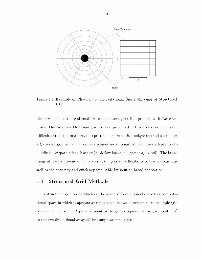
Figure 1.1: Example of Physical to Computational Space Mapping of StructuredGridthe ow. The existence of small cut cells, however, is still a problem with Cartesiangrids. The Adaptive Cartesian grid method presented in this thesis overcomes thedi�culties that the small cut cells present. The result is a unique method which usesa Cartesian grid to handle complex geometries automatically and uses adaptation tohandle the disparate length scales (both ow-based and geometry-based). The broadrange of results presented demonstrates the geometric exibility of this approach, aswell as the accuracy and e�ciency attainable by solution-based adaptation.1.1 Structured Grid MethodsA structured grid is one which can be mapped from physical space to a computa-tional space in which it appears as a rectangle, in two dimensions. An example gridis given in Figure 1.1. A physical point in the grid is represented as grid point (i; j)in the two dimensional array of the computational space.

41.1.1 Grid GenerationThe generation of a suitable starting grid using a body-�tted structured gridabout arbitrary bodies is a di�cult task. This is due to the fact that it is increas-ingly di�cult to maintain the structured cell numbering of the grid points. Forexample, one common organization of grid points dictates that i represents pointsaround the body while j represents points radial to the body. For one body, thisorganization works well, but when multiple bodies exist, it becomes increasinglydi�cult to maintain.Two standard methods are commonly used for generating these body-�tted struc-tured grids: elliptic and algebraic grid generation. Elliptic grid generation is doneby solving Laplace's or Poisson's equation, which smoothes the boundary data overthe domain [28, 58]. Using the proper boundary conditions, the grid lines representstreamlines and potential lines of potential ow. The quality of the grids generatedand the robustness of this method have made it popular for generating grids aboutsimple geometries. An excellant review of PDE-based techniques is given by Eise-man [19]. Algebraic grid generation is based on the idea of a smooth interpolationbetween points on boundary curves, for example, trans�nite interpolation [18]. Al-gebraic grid generation methods are faster than elliptic ones, but are not as easilyautomated. However, algebraic methods provide more control over the boundaries ofthe grid, which in turn allows an easier extension to multiblock methods. These twomethods are not viable options for complex geometries, but they can each be usedas building blocks for the newer multiblock [16] or patched-grid [46] methods. Multi-blocking dictates that the physical domain is carved up into simple subdomains, orblocks, where elliptic grid generation yields satisfactory results. The di�erent blocksare then linked together. The multiblocking is not unique, and how a ow is blocked

5can greatly a�ect the quality of the grid. The work required to generate these gridsincreases as the complexity of the bodies increase. A way is needed to automate theblocking procedure for structured methods to be viable.1.1.2 Grid AdaptationBoth grid-point redistribution and grid embedding have been employed on struc-tured grids [15, 19, 57]. Structured grids are especially well suited to grid-pointredistribution. The solution to the governing equations is computed on a grid whichis composed of a �xed number of points, redistributed from their original positionssuch that they congregate in the vicinity of ow features. The desired result is thebest solution possible for a �xed amount of resources. Possible point moving schemesinclude a spring analogy [39] and forcing function terms in the grid generation equa-tions [27]. As an example, if the shaded region in part (a) of Figure 1.2 requiresre�nement, part (b) gives the resulting grid after the grid-point redistribution. Al-ternatively, the grid in part (c) is the result of grid embedding. Adding a pointrequires adding the entire line on which the point lies. Unfortunately, many of thesenew grid points may not be needed. For this reason, grid embedding is generally notpractical for simple structured grids. More sophisticated structured grids which bothovercome this grid embedding di�culty and also allow more complicated geometriesinclude multi-block [16] and patched-grid [46] methods. Another variation is a tree ofstructured grids in which a region of the initial structured grid is re�ned by creatinga structured grid with a �ner resolution which is a child of the initial grid [6, 45].1.2 Unstructured Grid MethodsAn unstructured grid is one in which there is no mapping from the physical spaceto a simple computational space. Connectivity information must be stored, relating,

6i

j

(a) (b) (c)Figure 1.2: Re�nement of a Structured Gridfor instance, cells to the vertices that de�ne them. A variety of data structures arepossible [31, 51, 52], and the choice of data structure will a�ect the implementationof the grid generation process. Body-�tted unstructured grids are discussed below.1.2.1 Grid GenerationThe simplest form of body-�tted unstructured grid is one which is based on astructured grid [14, 47, 55]. The grid generation is achieved by destructuring astructured grid, as shown in Figure 1.3. The method works well for simple geometrieswhere a structured grid is readily available, but when arbitrarily complex bodies areneeded a more sophisticated method is needed.One sophisticated grid generation scheme is the Advancing Front method [14, 32,43]. First, a list of frontal faces is created between boundary nodes. The smallestface typically becomes the start of the front. An ideal third node is created fromthis face and put in a new list of nodes. Then, all other nodes in the triangulationare sorted by their distance from the new node and added to the list. The �rst nodeon the list which creates a triangle without crossing existing faces is used. The frontis then updated, and the process repeated until completion. This method requiresa lot of sorting and searching, inherently an O (N2) operation. More sophisticated

7Structured Grid

Unstructured GridFigure 1.3: Destructuring of a Structured Griddata structures used for searching can bring the costs down close to O (N logN).The grid created is usually smoothed with a Laplacian �lter, resulting in a grid witha high degree of regularity.Another sophisticated grid generation scheme is a Delaunay triangulation [3,25, 34, 48, 49]. Delaunay alone is not a complete scheme, but only a method oftriangulating a given set of points. One way to automate the introduction of pointsand create a Delaunay triangulation is �rst to triangulate the boundary nodes [23].The Delaunay triangulation of these points is taken as the initial grid. Cells with ahigh skewness are then re�ned by the insertion of a new node at the circumcenterof that triangle, followed by retriangulation. This procedure is costly, however, sinceskewness is a di�cult value to obtain. The Delaunay triangulation itself beginsby dividing the domain into Voronoi regions. The Voronoi region for a given nodeconsists of the part of the plane which is closer to that node than any other. A uniquetriangulation results when nodes whose Voronoi regions share a common boundaryare connected. This triangulation is optimal in the sense that the minimum angle is

8maximized in any triangle for all possible choices of diagonals between four convexnodes.A new development is a combination of Advancing Front and Delaunay methodsinto a \Frontal-Delaunay" method [37]. Grids with a high directional skewness canbe created for use with Navier-Stokes solvers, while some properties of Delaunaygrids are maintained.1.2.2 Grid AdaptationGrid-point redistribution can also be useful for unstructured grids, but it is di�-cult to maintain properties of a \good" grid, speci�cally grid skewness. One popularmethod of adaptation uses a spring analogy to determine node movement [26, 41].Unstructured grids are ideally suited for grid embedding. In areas where adapta-tion is needed, a cell is divided, or replaced by a number of smaller cells. Since the gridis unstructured, the change to the grid is purely local. The main di�culty is to de-termine when and where to re�ne. A number of di�erent re�nement criterion may beused which in some way use an estimate of the solution error. Then a threshold for re-�nement is set either by experience or by information obtained from the distributionof the error. Re�nement of this type has been carried out on triangular/tetrahedralgrids [34, 43, 64] and quadrilateral/hexahedral grids [7, 17, 36, 40, 59, 64] or a mixtureof both [38, 47]. This re�nement is most often isotropic, but anisotropic (directional)re�nement is also a viable option. [1, 14, 24, 55].1.3 Cartesian Grid MethodsAn approach which is becoming more popular is the use of non-body-�tted un-structured grids, speci�cally Cartesian grids, in which the bodies are \cut" out ofthe grid. A sample grid is shown for the leading edge of an airfoil in Figure 1.4. This

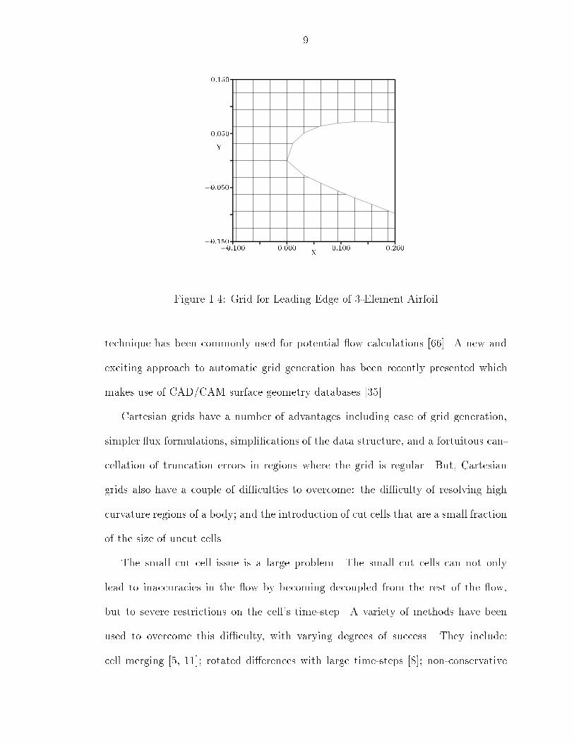
9�0:100 0:000 0:100 0:200�0:150�0:0500:0500:150

XYFigure 1.4: Grid for Leading Edge of 3-Element Airfoiltechnique has been commonly used for potential ow calculations [66]. A new andexciting approach to automatic grid generation has been recently presented whichmakes use of CAD/CAM surface geometry databases [35].Cartesian grids have a number of advantages including ease of grid generation,simpler ux formulations, simpli�cations of the data structure, and a fortuitous can-cellation of truncation errors in regions where the grid is regular. But, Cartesiangrids also have a couple of di�culties to overcome: the di�culty of resolving highcurvature regions of a body; and the introduction of cut cells that are a small fractionof the size of uncut cells.The small cut cell issue is a large problem. The small cut cells can not onlylead to inaccuracies in the ow by becoming decoupled from the rest of the ow,but to severe restrictions on the cell's time-step. A variety of methods have beenused to overcome this di�culty, with varying degrees of success. They include:cell merging [5, 11]; rotated di�erences with large time-steps [8]; non-conservative

10�0:100 0:000 0:100 0:200�0:150�0:0500:0500:150

XYFigure 1.5: Grid for Leading Edge of 3-Element Airfoil with Curvature Adaptationextrapolations [20]; volume of uid redistributions [42]; and a linear reconstructionwith local time-stepping [13, 17].1.4 A NewApproach - The Adaptive Cartesian Grid MethodAn adaptive Cartesian method combines the best elements of structured, unstruc-tured, and Cartesian grids. One element is a fortuitous cancellation of truncationserrors in regions where the grid is regular, as in structured grids. A Cartesian gridcan also be easily generated about any arbitrary geometric con�guration; at least aseasily as an unstructured grid. And, by applying adaptation to the resulting Carte-sian grid, both the geometry-based and solution-based length scales can be properlyresolved.The main di�culty lies in creating a ow solver which �ts into this approach. Itmust not only handle the di�erences in cell level, but also accurately address the cutcells. This includes the somewhat troublesome cut cells which are several orders of

11magnitude smaller in area than their uncut neighbor cells.An early Euler solver based on central-di�erencing on Cartesian grids was de-veloped by Clarke et al [11]. Body curvature resolution was achieved by clusteringthe grid lines near the areas of interest. Cut cells with an area less than 25% - 50%of uncut neighbor cells were merged into adjacent cells away from the body. Thesolutions obtained were poor near highly curved regions of the body and not smoothalong cut cells. Another central-di�erencing method was used by Epstein et al [20].Here, resolution was achieved by local grid re�nement. Cut cells were handled by anon-conservative extrapolation procedure. These solutions resolved body curvature,but did not adequately address cut cell boundary conditions.The �rst upwind-di�erencing method of the Euler equations on an adaptively-re�ned Cartesian grid was developed by Berger and LeVeque [8]. They addressedunsteady ows by using a rotated di�erence scheme with large time-steps on smallcells. Adaptation was achieved through local uniform �ne grid patches, which wererecursively nested. This approach works for cut cells with area greater than a fewpercent of uncut cells, but a special cell merging procedure was need for the very smallcells. A related unsteady solution method was developed by Pember et al [42]. Again,adaptation was achieved by re�ned patches of the grid. Cut cells were addressed bya \volume-of- uid redistribution" to eliminate time step restrictions. This methodhas problems with this type of boundary condition on small cut cells.In the work presented in this thesis, cell adaptation is applied to resolve properlyboth body curvature and ow features. This adaptation is no longer \block" adapta-tion, but rather \cell" adaptation, allowing more e�cient resolution of features thatare not aligned with the grid. Cut cells are handled by a linear reconstruction methoddesigned for unstructured grids combined with local time-stepping. Arbitrarily small

12cut cells now require no special treatment.The method speci�cally consists of a Cartesian grid with an unstructured cell-based data structure. Initial grid generation is enhanced by geometry-based re-�nement [38]. Solution adaptation is achieved by solution-based gradient informa-tion [40, 64]. The ow solver is based on the MUSCL concept [60], with a linearreconstruction technique [4], and either Roe's approximate Riemann solver [50] orVan Leer's ux splitting [30]. The solution is advanced in time by a multi-stage timestepping scheme [54, 62] with multigrid convergence acceleration [9].The data structure and grid generation are discussed in Chapter II. Each elementof the ow solver, including some accuracy studies, are examined in Chapter III.Chapter IV discusses the results for a variety of test cases. Finally, in Chapter V, asummary of the work presented is given, along with some conclusions and directionsfor future work.

CHAPTER IIDATA STRUCTURE AND GRIDGENERATION2.1 Quadtree Data StructureThe data structure of a code is the roadmap of the information contained inthe code. It shows what information is stored, and how to access it. For a typicalstructured-grid code, the data structure can be wholly contained in an (i; j) index.Unstructured-grid codes usually have a signi�cantly more complicated data structure.Of primary concern is the connectivity of the grid. Some information must be storedto determine which cells are neighbors of a given cell. A commonmethod of achievingthis is a linked list. For each cell, a list is stored of neighboring cells or faces,for example, implemented as array indices in FORTRAN or memory addresses inC. For many unstructured-grid schemes, this is the only option to determine cellconnectivity. Some schemes, however, allow the use of a data tree to achieve this goal.Other features of the code will determine whether the linked list or tree structurewill be the more e�cient choice.A quadtree-based structure is ideally suited for the Cartesian grid scheme imple-mented here. Like any true tree structure, it begins with one \root" cell. The rootcell is said to be at level 0. When this cell is re�ned, four children cells of equal size13

14Tree GridLevel

4

3

2

1

0

A

A

B

B

C

C

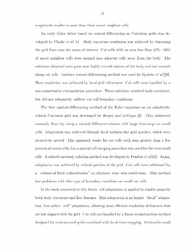
Figure 2.1: Quadtree Structureare created at one level higher, level 1. In turn, these cells are re�ned again untila suitable grid has been created. Each cell has a pointer to its parent and its fourchildren, if they exist. From this basic structure, all other needed information aboutthe relative position of any cell can be determined. This concept is illustrated inFigure 2.1.This tree structure has many inherent advantages over a linked list. One ofthe most important advantages is that a tree-based structure is well-suited to multi-grid [22]. A multigridmethod relies on a sequence of coarser grids. The low-frequencyerrors on a given grid become higher-frequency errors when passed to a coarser grid,and can then be more easily damped out. With the tree-based structure, thesecoarser grids already exist, and the communication between levels follows the exist-ing parent/child tree relationship. Multigrid implementation in a linked list requiresthe generation of multiple grids and special communication to relate the informationbetween the grids. This process is di�cult at best using a linked list.Another very important advantage of a tree-based data structure is the ease

15with which cells can be re�ned or coarsened. For a cell to be re�ned, the childrenpointers which were previously empty would now point to the four newly createdchildren cells. Using a linked list would require an additional check to see if thereare any neighbors which need their neighbor links updated to match these new cells.Coarsening a cell is also a very simple process in a tree structure. The cell simplyremoves the pointers to its four children. This assumes that the children cells do nothave children themselves. In a linked list, the e�ect this has on all neighboring cellsmust be determined. Another inherent advantage to a data tree is the amount ofinformation which can be obtained simply from the tree. Much of this informationis obtained by determining the level of a cell, or the number of successive parents tothe root cell. For example, the area of an uncut cell is simply a function of the rootcell area and the cell's level Ac = Aroot4level : (2.1)Neighbors in a tree structure are determined from the data tree, rather thandirectly stored in a linked list structure. To determine a cell's neighbor, the parentsare recursively queried as to whether one of its other children is that neighbor. In thebest case, �nding a cell's neighbor requires simply querying its parent for the locationof one of its other children. In the worst case, the tree must be traversed all the wayto the root and back to �nd the neighbor. In general, �nding the neighbor usuallyinvolves querying the cell's parent and grand-parent, since the expected number oflevels asymptotes to E (nlev) = 12 + 12 �22 + 12 �32 : : := X k2k� 2 (2.2)

16for �nding neighbors in the four primary directions. Thus, the neighbor is usually agrandchild of the cell's grandparent. The expected number of levels asymptotes to83 for �nding neighbors in all eight directions (horizontal, vertical, and diagonal). Asan example, the pseudo-code for �nding the North neighbor of a cell is listed below.NorthNeighbor(cellA)cellB = parent of cellAif cellA is SW child of cellB, thenNorthNeighbor = NW child of cellBif cellA is SE child of cellB, thenNorthNeighbor = NE child of cell Bif cellA is NE child of cellB, thencellC = NorthNeighbor(cellB)NorthNeighbor = SE child of cellCif cellA is NW child of cellB, thencellC = NorthNeighbor(cellB)NorthNeighbor = SW child of cellCFigure 2.2 shows the tree paths taken for �nding a North neighbor which requiredi�erent numbers of levels.Although the data tree is the most important part of this data structure, it isnot the only part. Cell type classi�cation must be provided by the data structure.It must also provide a means for storing and retrieving information about cells cutby a body. An integer value is used for each cell which records the cell type. For cutcells, that type is a two digit number which is encoded with information regardingwhich of its faces has been cut by the body. Each face of a cut cell is divided intotwo segments, so that the cell is made up of eight segments, numbered clockwisefrom the left segment of the top face. Then the �rst digit in the cell type is the �rstface of the cut and the second digit the second face of the cut. The �rst and secondcuts are determined by their clockwise order. Figure 2.3 shows a few cut cells andthe resulting cell types. For those cut cells, the coordinates of the cut location, or

17

North Neighbor of C3Levels

CC*

North Neighbor of B2 Levels

BB*

North Neighbor of A1 Level

AA*

TreeLevel

4

3

2

1

0

BC

Grid

B*C*A

A*

Figure 2.2: Tree Paths for Various North Neighbors

18Type = 45 Type = 25

type = 64Type = 62

1 2

3

4

56

7

8

Type = 37Figure 2.3: Various Cut-Cell Cell Typesnode, also needs to be stored, as well as a link between the cut cell and the correctcut node number.Since this data structure requires that some information be computed whenneeded, it is important to see that computing this information does not take somuch time as to eliminate the e�ectiveness of the data tree approach. Note thathow much time a speci�c piece requires to compute will be highly dependent uponthe speci�c programming implementation. The time to compute di�erent pieces ofinformation is not �xed. A good example is the time to compute the level of a cell.This is a very simple procedure, but the level of a cell is used many, many times.If the cell level is computed when it is needed, that computation takes 10% of thetotal time. On the other hand, if the cell level is computed once and stored, onlyone integer of storage per cell is needed. Determination of the neighbors of a cellis another necessary procedure. If a cell's neighbors are computed when needed, ittakes 10-15% of the total time. Storing that information requires up to 10 integersof storage per cell. Based on these kinds of comparisons, the cell level is stored and

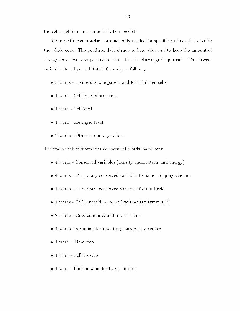
19the cell neighbors are computed when needed.Memory/time comparisons are not only needed for speci�c routines, but also forthe whole code. The quadtree data structure here allows us to keep the amount ofstorage to a level comparable to that of a structured grid approach. The integervariables stored per cell total 10 words, as follows;� 5 words - Pointers to one parent and four children cells� 1 word - Cell type information� 1 word - Cell level� 1 word - Multigrid level� 2 words - Other temporary valuesThe real variables stored per cell total 31 words, as follows;� 4 words - Conserved variables (density, momentum, and energy)� 4 words - Temporary conserved variables for time stepping scheme� 4 words - Temporary conserved variables for multigrid� 4 words - Cell centroid, area, and volume (axisymmetric)� 8 words - Gradients in X and Y directions� 4 words - Residuals for updating conserved variables� 1 word - Time step� 1 word - Cell pressure� 1 word - Limiter value for frozen limiter

20Since only the integer storage is associated with the data structure, this code requiresnearly the same amount of memory as a structured grid code implementing the same ow solver strategy. On the other hand, the data structure imposes a 30% overheadfor the total time to run the code, with neighbor �nding accounting for half of thatoverhead. This run-time cost is o�set by the fact that this method can produce upto an order of magnitude reduction in the number of cells needed due to adaptation.2.2 Generating The Initial GridIn the generation of a suitable grid, the �rst step is the generation of an initialgrid. To generate the initial grid, certain information is needed from the user of theprogram. In the approach developed in this work, all that is needed is the location ofthe outer boundaries, the cell aspect ratio, and a desired minimum grid resolution.Then, this information in hand, the generation of a suitable initial grid can proceed.The outer boundary information used is in the form of an X coordinate at the leftand right boundary,XL and XR, and a Y coordinate at the bottom and top boundary,YB and YT . The cell aspect ratio and minimum grid resolution are speci�ed by givingthe number of cells in each direction,M in the X direction and N in the Y direction.Once this information is known, the exact size and location of the root cell can bedetermined. First, the size of a cell at the given minimum grid resolution is �Xc by�Yc de�ned as �Xc = XR �XLM�Yc = YT � YBN : (2.3)Next, since the ow is surrounded by a ring of boundary cells at the minimum gridresolution, the left X and bottom Y values of the root cell are set asXLroot = XL ��XcYBroot = YB ��Yc : (2.4)

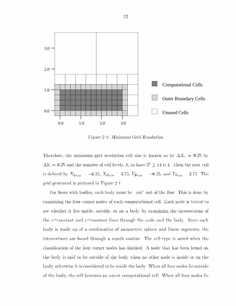
21Now, since successively re�ning a root cell and its children will give possible uniformgrid resolutions of 1, 2, 4, 8, 16, ... ,2k, etc., the smallest value of k that satis�es2k � max (M;N) + 2 must be found. With k known, the right X and top Y valuesof the root cell become XRroot = XLroot + 2k�XcYTroot = YBroot + 2k�Yc : (2.5)At this point, all the attributes of the root cell can be set. Its location and size areknown, and cell level is set to zero. Now that the �rst cell is completed, all cellswithout children which lie within the outer boundaries are recursively re�ned untilthe cells reach a level equal to k. By just re�ning cells within the outer boundaries,the number of cells that will never be used because they are outside of the ow�eldis reduced. Finally, all cells at level k that are within the box described byXL ��Xc � X � XR +�XcYB ��Yc � Y � YT +�Yc (2.6)are agged as cells in the ow�eld. All other cells are marked as unused cells whichjust complete the data tree. Of the cells in the ow�eld, cells withinXL � X � XRYB � Y � YT (2.7)are speci�cally marked to be computational cells and the rest of the ow�eld cells tobe outer boundary ghost cells.The grid generation for an arbitrary channel ow can serve as an example. Theuser has speci�ed the following:XL = 0:0 ; XR = 3:0YB = 0:0 ; YT = 1:0M = 12 ; N = 4 (2.8)

220.0 1.0 2.0 3.0

0.0

1.0

2.0

3.0

Outer Boundary Cells

Unused Cells

Computational Cells

Figure 2.4: Minimum Grid ResolutionTherefore, the minimum grid resolution cell size is known to be �Xc = 0:25 by�Yc = 0:25 and the number of cell levels, k, to have 2k � 14 is 4. Then the root cellis de�ned by XLroot = �0:25, XRroot = 3:75, YBroot = �0:25, and YTroot = 3:75. Thegrid generated is pictured in Figure 2.4.For ows with bodies, each body must be \cut" out of the ow. This is done byexamining the four corner nodes of each computational cell. Each node is tested tosee whether it lies inside, outside, or on a body by examining the intersections ofthe x=constant and y=constant lines through the node and the body. Since eachbody is made up of a combination of parametric splines and linear segments, theintersections are found through a search routine. The cell type is saved when theclassi�cation of the four corner nodes has �nished. A node that has been found onthe body is said to be outside of the body when no other node is inside or on thebody, otherwise it is considered to be inside the body. When all four nodes lie outsideof the body, the cell becomes an uncut computational cell. When all four nodes lie

23inside of the body, the cell becomes an unused cell just �lling the data tree. All othercombinations imply a cell which has been cut by the body. The cut locations arestored using the x=constant and y=constant intersection information. From here onout, each new cell is classi�ed and checked for body cuts as soon as it is created.2.3 Geometry AdaptationOnce the initial grid has been generated and the cells all classi�ed, the grid isimproved through a series of three geometry-based adaptations: all-cell adaptation;cut-cell adaptation; and curvature-cell adaptation. The amount of each type ofadaptation is determined by individual cell length scale parameters given by the user.The cumulative e�ect of these procedures is a suitable grid for the computation of a ow solution.In all-cell adaptation, all computational cells are re�ned until their length scale,the minimum of �x and �y, is less that the length scale provided by the user forthis type of adaptation. The minimum grid resolution is already known from thegeneration of the initial grid, but the user may wish to begin ow calculation on a�ner grid, particularly for use with the multigrid convergence acceleration describedin Section 3.3.Cut-cell adaptation is similar to all-cell adaptation. The di�erence is that cells cutby the body will be re�ned if their length scale is less than the cut-cell length scale.Another di�erence is that when a cell is agged for re�nement, all of its neighborsare also re�ned. Re�ning the neighbors ensures a smoother transition from the �nercells on the body to the coarser cells away from the body.Once cut-cell adaptation has �nished, curvature-cell adaptation begins. Thisprocess begins by examining two neighboring cut cells and comparing the slope ofthe body face on each cell. If the di�erence in the slopes is above a threshold value,the cells and their neighbors are agged for re�nement. The actual check used to

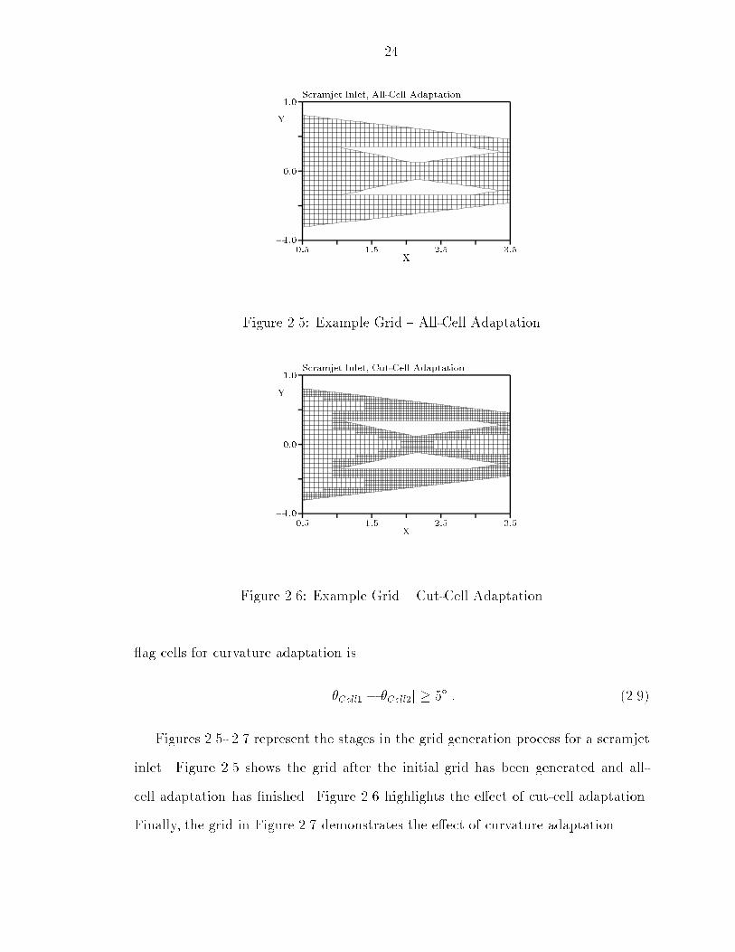
240:5 1:5 2:5 3:5�1:00:01:0 XY Scramjet Inlet, All-Cell Adaptation.

Figure 2.5: Example Grid { All-Cell Adaptation0:5 1:5 2:5 3:5�1:00:01:0 XY Scramjet Inlet, Cut-Cell Adaptation.

Figure 2.6: Example Grid { Cut-Cell Adaptation ag cells for curvature adaptation isj�Cell1 � �Cell2j � 5� : (2.9)Figures 2.5- 2.7 represent the stages in the grid generation process for a scramjetinlet. Figure 2.5 shows the grid after the initial grid has been generated and all-cell adaptation has �nished. Figure 2.6 highlights the e�ect of cut-cell adaptation.Finally, the grid in Figure 2.7 demonstrates the e�ect of curvature adaptation.

250:5 1:5 2:5 3:5�1:00:01:0 XY Scramjet Inlet, Curvature-Cell Adaptation.

Figure 2.7: Example Grid { Curvature-Cell Adaptation2.4 Solution AdaptationIn addition to all-cell, cut-cell, and curvature-cell adaptation, the grid is alsomodi�ed by solution-based adaptation. The cells in the grid are either re�ned orcoarsened based on the characteristics of the ow. This takes place only after asolution is su�ciently converged. At that point, cells are agged for re�nement orcoarsening based on a given adaptation criterion. That criterion should detect anydiscontinuity in the ow. For inviscid compressible ow, the important discontinuitiesare shocks, shear layers, and contact surfaces.Typically, the criterion of choice has been a density, pressure, or total-velocitydi�erence. However, since the density and pressure di�erences have di�culty detect-ing shear layers, di�erences of total velocity have been most often used. Even so,the total-velocity di�erence has trouble di�erentiating between features of di�erentstrengths, such as a strong shock and a weaker shear. The total-velocity di�erencecriterion will be compared to a new adaptation criterion based on the curl and di-vergence of velocity. This new criterion e�ectively detects each discontinuity andminimizes the di�erences in the relative strengths of di�erent discontinuities. Thestrengths and weaknesses of various criteria are listed in Table 2.1.

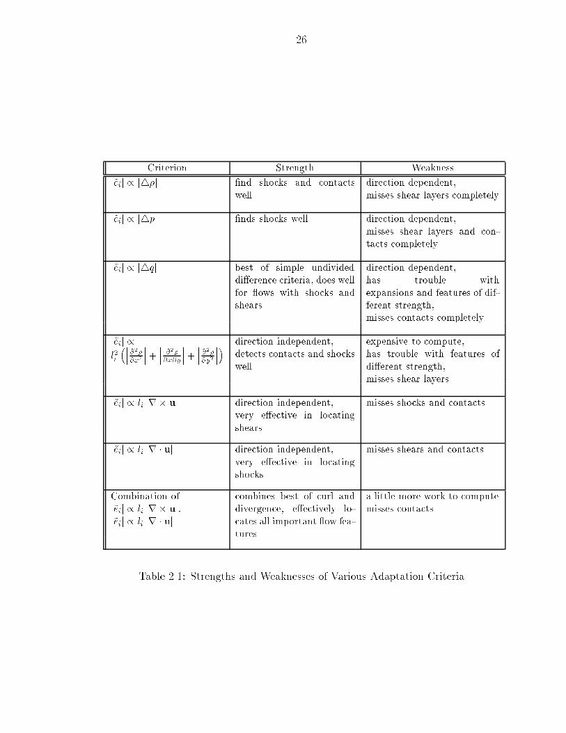
26Criterion Strength Weaknessj~eij / j4�j �nd shocks and contactswell direction dependent,misses shear layers completelyj~eij / j4pj �nds shocks well direction dependent,misses shear layers and con-tacts completelyj~eij / j4qj best of simple undivideddi�erence criteria, does wellfor ows with shocks andshears direction dependent,has trouble withexpansions and features of dif-ferent strength,misses contacts completelyj~eij /l2i ����@2�@x2 ���+ ��� @2�@x@y ���+ ��� @2�@y2 ���� direction independent,detects contacts and shockswell expensive to compute,has trouble with features ofdi�erent strength,misses shear layersj~eij / li jr � uj direction independent,very e�ective in locatingshears misses shocks and contactsj~eij / li jr � uj direction independent,very e�ective in locatingshocks misses shears and contactsCombination ofj~eij / li jr � uj,j~eij / li jr � uj combines best of curl anddivergence, e�ectively lo-cates all important ow fea-tures a little more work to computemisses contactsTable 2.1: Strengths and Weaknesses of Various Adaptation Criteria

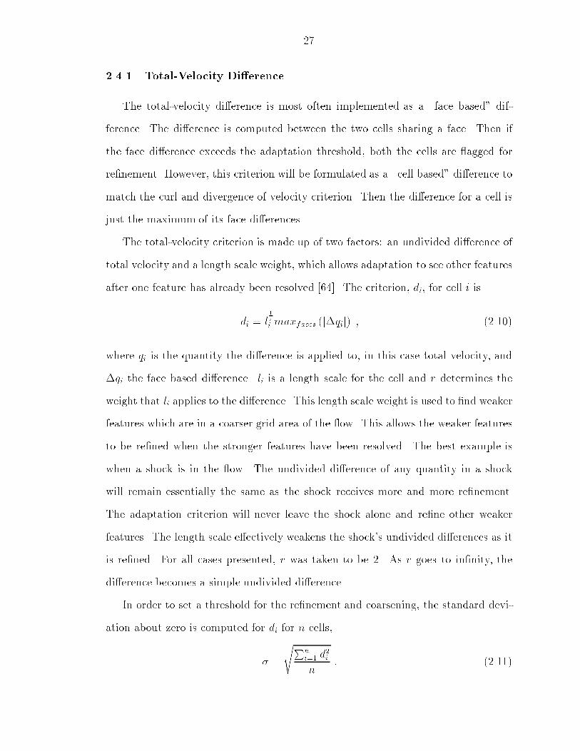
272.4.1 Total-Velocity Di�erenceThe total-velocity di�erence is most often implemented as a \face based" dif-ference. The di�erence is computed between the two cells sharing a face. Then ifthe face di�erence exceeds the adaptation threshold, both the cells are agged forre�nement. However, this criterion will be formulated as a \cell based" di�erence tomatch the curl and divergence of velocity criterion. Then the di�erence for a cell isjust the maximum of its face di�erences.The total-velocity criterion is made up of two factors: an undivided di�erence oftotal velocity and a length scale weight, which allows adaptation to see other featuresafter one feature has already been resolved [64]. The criterion, di, for cell i isdi = l 1ri maxfaces (j�qij) ; (2.10)where qi is the quantity the di�erence is applied to, in this case total velocity, and�qi the face based di�erence. li is a length scale for the cell and r determines theweight that li applies to the di�erence. This length scale weight is used to �nd weakerfeatures which are in a coarser grid area of the ow. This allows the weaker featuresto be re�ned when the stronger features have been resolved. The best example iswhen a shock is in the ow. The undivided di�erence of any quantity in a shockwill remain essentially the same as the shock receives more and more re�nement.The adaptation criterion will never leave the shock alone and re�ne other weakerfeatures. The length scale e�ectively weakens the shock's undivided di�erences as itis re�ned. For all cases presented, r was taken to be 2. As r goes to in�nity, thedi�erence becomes a simple undivided di�erence.In order to set a threshold for the re�nement and coarsening, the standard devi-ation about zero is computed for di for n cells,� = sPni=1 d2in : (2.11)

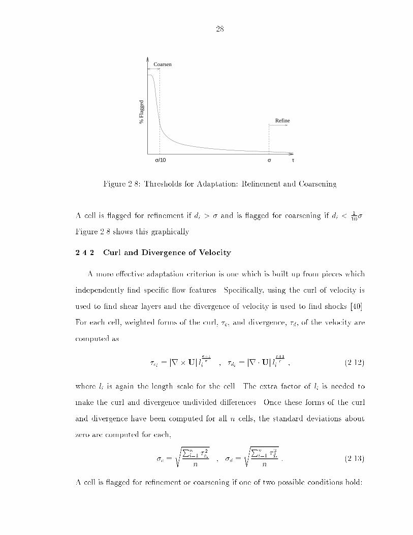
28Coarsen

σ/10 σ τ

% F

lagg

ed

RefineFigure 2.8: Thresholds for Adaptation: Re�nement and CoarseningA cell is agged for re�nement if di > � and is agged for coarsening if di < 110�.Figure 2.8 shows this graphically.2.4.2 Curl and Divergence of VelocityA more e�ective adaptation criterion is one which is built up from pieces whichindependently �nd speci�c ow features. Speci�cally, using the curl of velocity isused to �nd shear layers and the divergence of velocity is used to �nd shocks [40].For each cell, weighted forms of the curl, �c, and divergence, �d, of the velocity arecomputed as �ci = jr�Uj l r+1ri ; �di = jr �Uj l r+1ri ; (2.12)where li is again the length scale for the cell. The extra factor of li is needed tomake the curl and divergence undivided di�erences. Once these forms of the curland divergence have been computed for all n cells, the standard deviations aboutzero are computed for each,�c = sPni=1 � 2cin ; �d = sPni=1 � 2din : (2.13)A cell is agged for re�nement or coarsening if one of two possible conditions hold:

291. if either �ci > �c or �di > �d, the cell is agged for re�nement,2. if both �ci < 110�c and �di < 110�d, the cell is agged for coarsening.For cases where the resolution of one feature is much more important than otherfeatures, the weights on the adaptation criterion can be changed. For example, if theresolution of a shear layer is vital while the shocks in the ow are not, cells could be agged for re�nement if �ci > 12�c or �di > 2�c. This ags more cells for re�nementbased on curl and less cells based on divergence, e�ectively weighting the shear layermore heavily.2.4.3 Comparison of Adaptation CriteriaThe adaptation criteria described above were tested on a variety of test cases,including a double wedge, a NACA airfoil, and an axisymmetric jet, among others.Of these, an axisymmetric jet will be examined �rst since it clearly highlights the dif-ferences of the adaptation criteria when shocks are present. Then a smooth subsonicNACA airfoil will be examined.The axisymmetric jet is made up of a nozzle of radius one which exits into thefreestream ow at X = 0:0. This ow has a freestream and jet Mach number of 1.25,a jet-to-stream total temperature ratio of 1.0, and a jet-to-stream total pressure ratioof 35.0. This particular jet ow has the following ow features: 1) an expansion outof the nozzle, 2) a curved shock emanating from the nozzle lip and re ecting atthe symmetry axis, 3) a shear separating the jet and the outer stream, and 4) anoblique shock through which the outer stream passes. A more detailed descriptionof the axisymmetric jet is found in Section 4.3. The grid and Mach contours for theconverged solution are shown in Figures 2.9 and 2.10.Figure 2.11 shows the cells that will be agged for re�nement based on totalvelocity. Notice that both the shear layer and the shocks get agged for re�nement.However, the shocks are not agged along their entire length. As the shock on

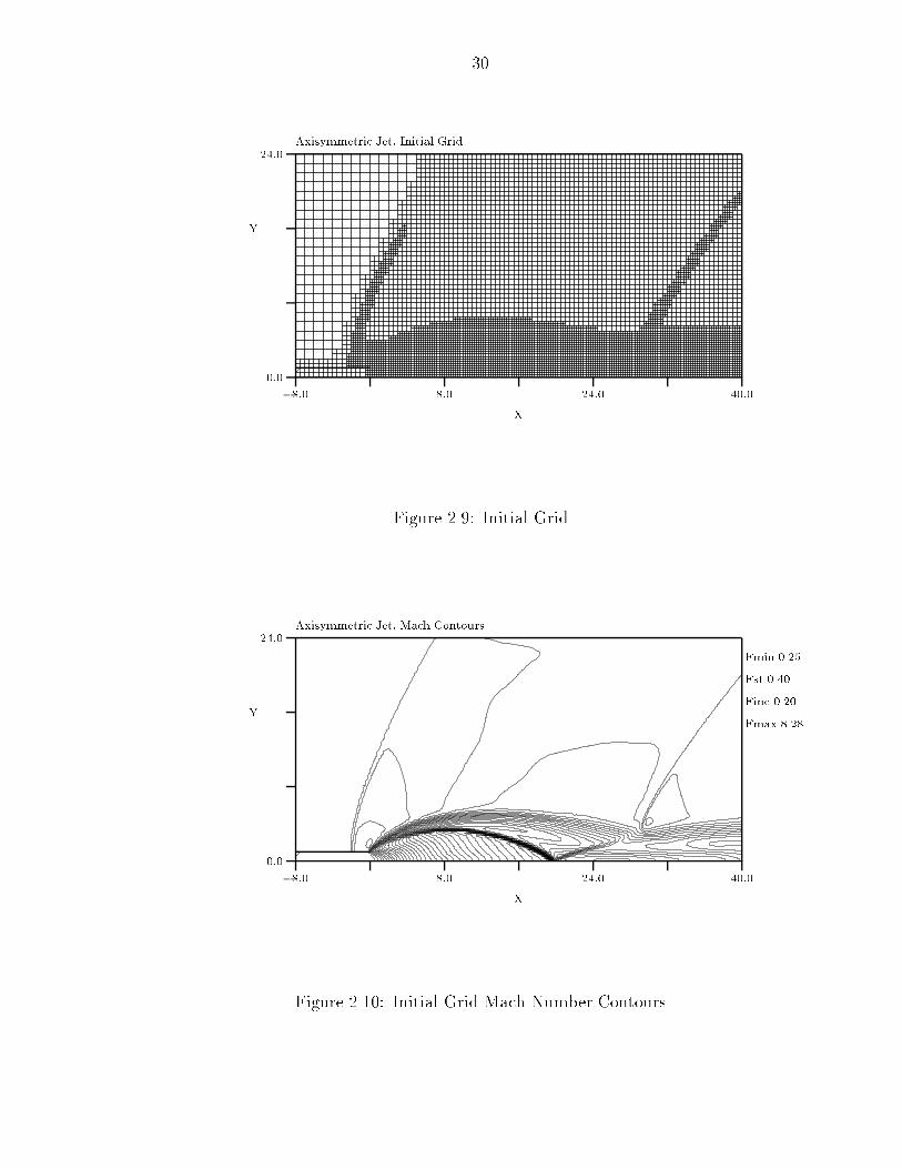
30�8:0 8:0 24:0 40:00:0

24:0X

Y Axisymmetric Jet, Initial Grid.Figure 2.9: Initial Grid

�8:0 8:0 24:0 40:00:024:0

XY Axisymmetric Jet, Mach Contours. Fmin 0.25Fst 0.40Finc 0.20Fmax 8.28

Figure 2.10: Initial Grid Mach Number Contours

31�8:0 8:0 24:0 40:00:0

24:0X

Y Axisymmetric Jet, Total Velocity Adaptation.1578 Cells Flagged, di > �Figure 2.11: Cells Flagged for Re�nement by Total-Velocity Re�nement, di > �the nozzle lip weakens, it does not generate enough total-velocity di�erence to be agged. Also, very little of the expansion at the nozzle lip which re ects o� the axisof symmetry is agged.In an e�ort to get these features agged for more e�cient re�nement, the adap-tation threshold can be lowered for re�ning cells. The plot for division based ondi > 12� is shown in Figure 2.12. Here the complete length of the shocks are agged,but the expansion fan is still missed. In addition, the number of cells agged hasnearly doubled, with only a little improvement in the cells agged.Figure 2.13 shows which cells will be agged for coarsening. A large portionof the expansion fan, and much of the outer stream ow, has been agged. Fromthese adaptation plots, it is obvious that in terms of total velocity di�erence, theshear layer is the strongest feature present, with the shocks a little weaker, and theexpansion fan much weaker than the shear.This variation in the relative strengths is easily taken care of with adaptationbased on the curl and divergence of velocity. The curl of the velocity very e�ectively

32�8:0 8:0 24:0 40:00:0

24:0X

Y Axisymmetric Jet, Total Velocity Adaptation.2546 Cells Flagged, di > 12�Figure 2.12: Cells Flagged for Re�nement by Total-Velocity Adaptation, di > 12�.

�8:0 8:0 24:0 40:00:024:0

XY Axisymmetric Jet, Total Velocity Adaptation.2292 Cells Flagged, di < 110�

Figure 2.13: Cells Flagged for Coarsening by Total-Velocity Adaptation, di < 110�.

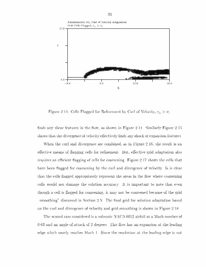
33�8:0 8:0 24:0 40:00:0

24:0X

Y Axisymmetric Jet, Curl of Velocity Adaptation.1148 Cells Flagged, �ci > �cFigure 2.14: Cells Flagged for Re�nement by Curl of Velocity, �ci > �c.�nds any shear features in the ow, as shown in Figure 2.14. Similarly Figure 2.15shows that the divergence of velocity e�ectively �nds any shock or expansion features.When the curl and divergence are combined, as in Figure 2.16, the result is ane�ective means of agging cells for re�nement. But, e�ective grid adaptation alsorequires an e�cient agging of cells for coarsening. Figure 2.17 shows the cells thathave been agged for coarsening by the curl and divergence of velocity. Is is clearthat the cells agged appropriately represent the areas in the ow where coarseningcells would not damage the solution accuracy. It is important to note that eventhough a cell is agged for coarsening, it may not be coarsened because of the grid\smoothing" discussed in Section 2.5. The �nal grid for solution adaptation basedon the curl and divergence of velocity and grid smoothing is shown in Figure 2.18.The second case considered is a subsonic NACA 0012 airfoil at a Mach number of0.63 and an angle of attack of 2 degrees. This ow has an expansion at the leadingedge which nearly reaches Mach 1. Since the resolution at the leading edge is not

34�8:0 8:0 24:0 40:00:0

24:0X

Y Axisymmetric Jet, Divergence of Velocity Adaptation.937 Cells Flagged, �di > �dFigure 2.15: Cells Flagged for Re�nement by Divergence of Velocity, �di > �d.

�8:0 8:0 24:0 40:00:024:0

XY Axisymmetric Jet, Curl and Divergence of Velocity Adaptation.2004 Cells Flagged, �ci > �c or �di > �d

Figure 2.16: Cells Flagged for Re�nement by Curl and Divergence of Velocity,�ci > �c or �di > �d.

35�8:0 8:0 24:0 40:00:0

24:0X

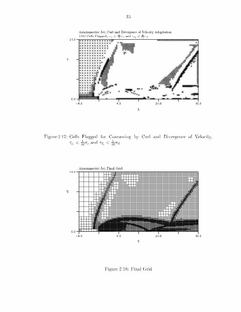
Y Axisymmetric Jet, Curl and Divergence of Velocity Adaptation.1195 Cells Flagged, �ci < 110�c and �di < 110 �dFigure 2.17: Cells Flagged for Coarsening by Curl and Divergence of Velocity,�ci < 110�c and �di < 110�d.

�8:0 8:0 24:0 40:00:024:0

XY Axisymmetric Jet, Final Grid.

Figure 2.18: Final Grid

36�1:0 0:0 1:0�1:00:0

1:0XY NACA 0012 Airfoil, Initial Grid.

Figure 2.19: Initial Gridquite su�cient, entropy is generated near the stagnation point, and convected overthe upper surface of the airfoil. Only the cells which are agged for re�nement willbe examined. Since this is an airfoil ow, the cells agged to coarsen will typicallybe those cells at a distance of about one or less chords from the airfoil. The grid andMach contours for this ow are pictured in Figures 2.19 and 2.20.Total-velocity adaptation will ag for re�nement the cells pictured in Figure 2.21.The re�nement is restricted to the area around the leading edge and the trailing edge.The entropy layer is not even seen.When the curl of velocity adaptation criterion is applied, the cells plotted inFigure 2.22 are agged for re�nement. Note that no curl should exist in the ow,but when an entropy layer exists, a small curl is found in that entropy layer. Thedivergence of velocity, on the other hand, ags the cells which are near the leadingand trailing edge stagnation and the expansion about the front portion of the airfoil.The divergence is pictured in Figure 2.23. The reason that this �gure may look alittle odd, is that the cell length scale weighting is coming into play. Cells with a

37�1:0 0:0 1:0�1:00:0

1:0XY NACA 0012 Airfoil, Mach Contours. Fmin 0.057Fst 0.080Finc 0.040Fmax 0.961

Figure 2.20: Initial Grid Mach Number Contours�1:0 0:0 1:0�1:00:0

1:0XY 461 Cells Flagged, di > �NACA 0012 Airfoil, Total Velocity Adaptation

Figure 2.21: Cells Flagged for Re�nement by Total-Velocity Re�nement, di > �

38�1:0 0:0 1:0�1:00:0

1:0XY 331 Cells Flagged, �ci > �cNACA 0012 Airfoil, Curl of Velocity Adaptation

Figure 2.22: Cells Flagged for Re�nement by Curl of Velocity, �ci > �c�1:0 0:0 1:0�1:00:0

1:0XY 729 Cells Flagged, �di > �dNACA 0012 Airfoil, Divergence of Velocity Adaptation

Figure 2.23: Cells Flagged for Re�nement by Divergence of Velocity, �di > �d

39�1:0 0:0 1:0�1:00:0

1:0XY 1002 Cells Flagged, �ci > �c and �di > �dNACA 0012 Airfoil, Curl and Divergence of Velocity Adaptation

Figure 2.24: Cells Flagged for Re�nement by Curl and Divergence of Velocity,�ci > �c or �di > �dlittle smaller divergence, but with a larger size, will more likely be agged. Thecombined e�ect of these two criteria is shown in Figure 2.24. When this combinede�ect is implemented, and the grid is smoothed, the grid pictured in Figure 2.25 isobtained.2.5 Grid \Smoothing"Any grid that has been generated by the method previously described could havecertain \undesirable features." Some are undesirable in that they would violate thedata structure; for others, allowing them would unnecessarily complicate the datastructure; still others are undesirable in that computational experience shows thatthey may degrade the solution somewhat in their vicinity. In order to remove thesefeatures, the grid is modi�ed by coarsening or re�ning individual cells to remove aparticular undesirable feature. This process is called \smoothing" the grid. Thisprocedure is recursive, and converges to a grid with no undesirable features. Grid

40�1:0 0:0 1:0�1:00:0

1:0XY NACA 0012 Airfoil, Final Grid.

Figure 2.25: Final Gridsmoothing is applied immediately following any major modi�cation to the grid andbefore the ow solver begins its operation. For example, the grid is smoothed after theinitial grid is created, after the geometry adaptation is done, after solution adaptationis �nished, and before the ow solver is applied.The features that the grid smoothing routine removes have changed considerablyas the speci�c implementations of the data structure and ow solver have changed.A good example of this is the need for removing cell level di�erences greater than onebetween neighboring cells. In an early version of the code, this was done because thedata structure was not general enough to represent grids with jumps in cell level. Ina later version, the data structure was generalized so that it was no longer necessaryto remove cell level di�erences by smoothing. But, it was then seen that this featurecan lead to a degradation of the solution in its vicinity. Thus the feature was thenreturned to the grid smoothing routine for removal. The features discussed beloware those currently \smoothed" from the grid.The most important smoothing takes place to remove features which would violate

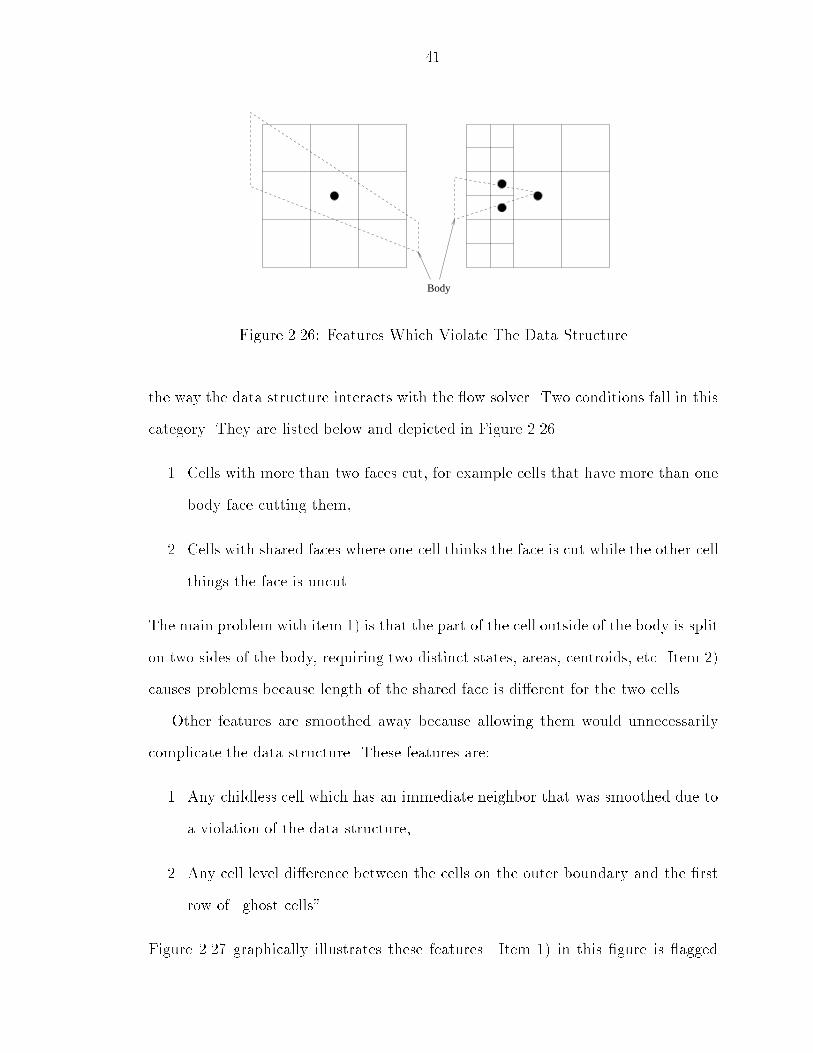
41BodyFigure 2.26: Features Which Violate The Data Structurethe way the data structure interacts with the ow solver. Two conditions fall in thiscategory. They are listed below and depicted in Figure 2.26.1. Cells with more than two faces cut, for example cells that have more than onebody face cutting them,2. Cells with shared faces where one cell thinks the face is cut while the other cellthings the face is uncut.The main problem with item 1) is that the part of the cell outside of the body is spliton two sides of the body, requiring two distinct states, areas, centroids, etc. Item 2)causes problems because length of the shared face is di�erent for the two cells.Other features are smoothed away because allowing them would unnecessarilycomplicate the data structure. These features are:1. Any childless cell which has an immediate neighbor that was smoothed due toa violation of the data structure,2. Any cell level di�erence between the cells on the outer boundary and the �rstrow of \ghost cells".Figure 2.27 graphically illustrates these features. Item 1) in this �gure is agged

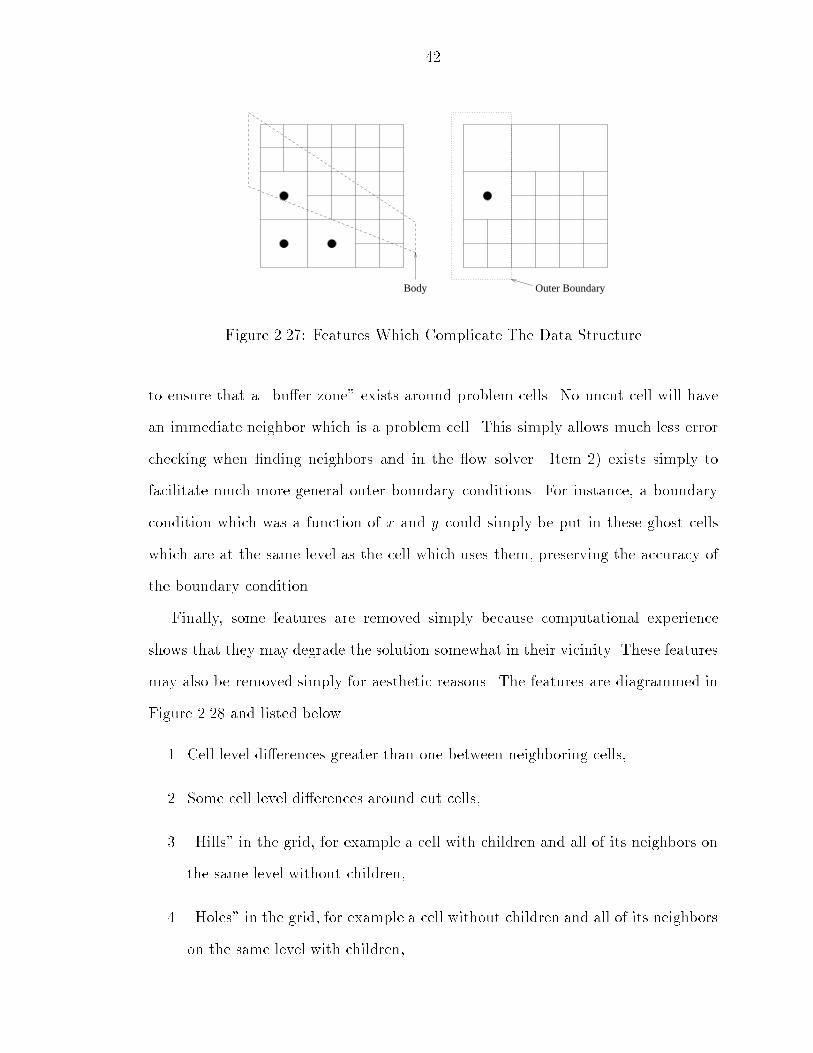
42Body Outer BoundaryFigure 2.27: Features Which Complicate The Data Structureto ensure that a \bu�er zone" exists around problem cells. No uncut cell will havean immediate neighbor which is a problem cell. This simply allows much less errorchecking when �nding neighbors and in the ow solver. Item 2) exists simply tofacilitate much more general outer boundary conditions. For instance, a boundarycondition which was a function of x and y could simply be put in these ghost cellswhich are at the same level as the cell which uses them, preserving the accuracy ofthe boundary condition.Finally, some features are removed simply because computational experienceshows that they may degrade the solution somewhat in their vicinity. These featuresmay also be removed simply for aesthetic reasons. The features are diagrammed inFigure 2.28 and listed below.1. Cell level di�erences greater than one between neighboring cells,2. Some cell level di�erences around cut cells,3. \Hills" in the grid, for example a cell with children and all of its neighbors onthe same level without children,4. \Holes" in the grid, for example a cell without children and all of its neighborson the same level with children,

43Body

Figure 2.28: Features Which Degrade The Solution AccuracyAs explained above, item 1) was originally a violation of the data structure. But,when that problem was removed, this feature was again agged for removal from thegrid because it harms the solution accuracy. A more gradual level change of cellshelps to remove \grid e�ects" from the solution. The reason item 2) is smoothedaway is similar to item 1). A steep level change of cells away from the body causeda deterioration of the solution in that region. Items 3) and 4) are almost purelyaesthetic considerations. They have very little e�ect on the solution accuracy, buthave a very large e�ect on how good the grid looks.To show the e�ect of these accuracy and aesthetic features, a 15 degree ramp ina channel is presented. The grid and Mach contours are shown in Figure 2.29. Thegrid has no aesthetic \trouble spots" and the Mach contours smoothly ow throughthe cell level changes. Figure 2.30 shows the grid and Mach contours without theaccuracy and aesthetic smoothing. This grid was intentionally modi�ed to show the

440:001:00Y Grid For Flow With Smoothing

0:00 1:00 2:00 3:000:001:00 XY Mach Contours For Flow With SmoothingFigure 2.29: Grid and Mach Contours With Accuracy And Aesthetic FeaturesSmoothed

450:001:00Y Grid For Flow Without Smoothing

0:00 1:00 2:00 3:000:001:00 XY Mach Contours For Flow Without SmoothingFigure 2.30: Grid and Mach Contours Without Accuracy And Aesthetic FeaturesSmoothedtype of grid which would be legal without the accuracy and aesthetic smoothing.Nevertheless, the Mach contours given are nearly identical to the smoothed ow, butwith a little deviation where neighboring cells are more than one cell level apart.It is possible for grid smoothing to \undo" some of the changes made by solutionadaptation. For instance, solution adaptation may require a particular cell to becoarsened while grid smoothing may want that same cell re�ned again. When thishappens, a small amount of detail may be lost. In order to avoid this problem, some\smoothing logic" has been put into the solution adaptation method. Thus, whensolution adaptation ags a cell for coarsening or re�nement, and it is obvious thatsmoothing will \undo" this operation, the cell is left as is. The simplest examplemay be when a cell with more than two cut faces exists. This particular undesirablefeature is removed by re�ning it and its eight neighbors. If it is determined that

46one of these nine cells should be coarsened, the cell is now left alone since that cellwould have been re�ned again in smoothing, no matter what other cells around itare re�ned or coarsened.

CHAPTER IIIFLOW SOLVERThe upwind �nite-volume ow solver is based on the work of Godunov [21]. Inthe original approach, the solution was considered to be piecewise constant over eachgrid cell at a �xed time. The evolution of the ow to the next time step results fromthe wave interactions originating at adjacent cell boundaries, speci�cally a Riemannproblem. In Riemann's initial-value problem, a membrane separating a gas at twodi�erent states is ruptured, and shock, contact, and expansion waves are emittedwhen the two states interact. The Riemann problem is pictured in Figure 3.1. Thisapproach leads to �rst order spatial accuracy.The Godunov approach was �rst extended to second-order spatial accuracy bythe MUSCL approach developed by Van Leer [60], made up of two decoupled stages.The �rst stage is the projection stage where the face values UL and UR are created.The second stage is the solution to the resulting Riemann problem. Using a linearapproximation of the solution on each cell for the projection stage leads to second-order spatial accuracy, while a quadratic representation on each cell leads to third-order spatial accuracy. In this work, a second-order spatial accuracy is achievedby a linear reconstruction procedure on each cell [4]. The e�ect on UL and UR bythis higher order reconstruction is pictured in Figure 3.2. Unfortunately, limitingis required to enforce the monotonicity of the reconstruction. Wherever limiting isused, the spatial accuracy of the projection is somewhat reduced, possibly to a �rst47

48L R

expansion contact shock

t

grid-normalFigure 3.1: The Riemann Problemnew U

old U R

R

new U

old U

L

LFigure 3.2: Linear Reconstruction for Higher Order UL and URorder spatial accuracy.The Euler ow solver described here consists of three primary components: alinear reconstruction procedure, for obtaining accurate, limited values of the owvariables at face midpoints; a ux formulation, for computing the ux through cell-faces; and a multi-stage time-stepping scheme using multigrid, for advancing thesolution to a steady state. The individual components of these procedures, alongwith some code accuracy and e�ciency considerations, are described below.

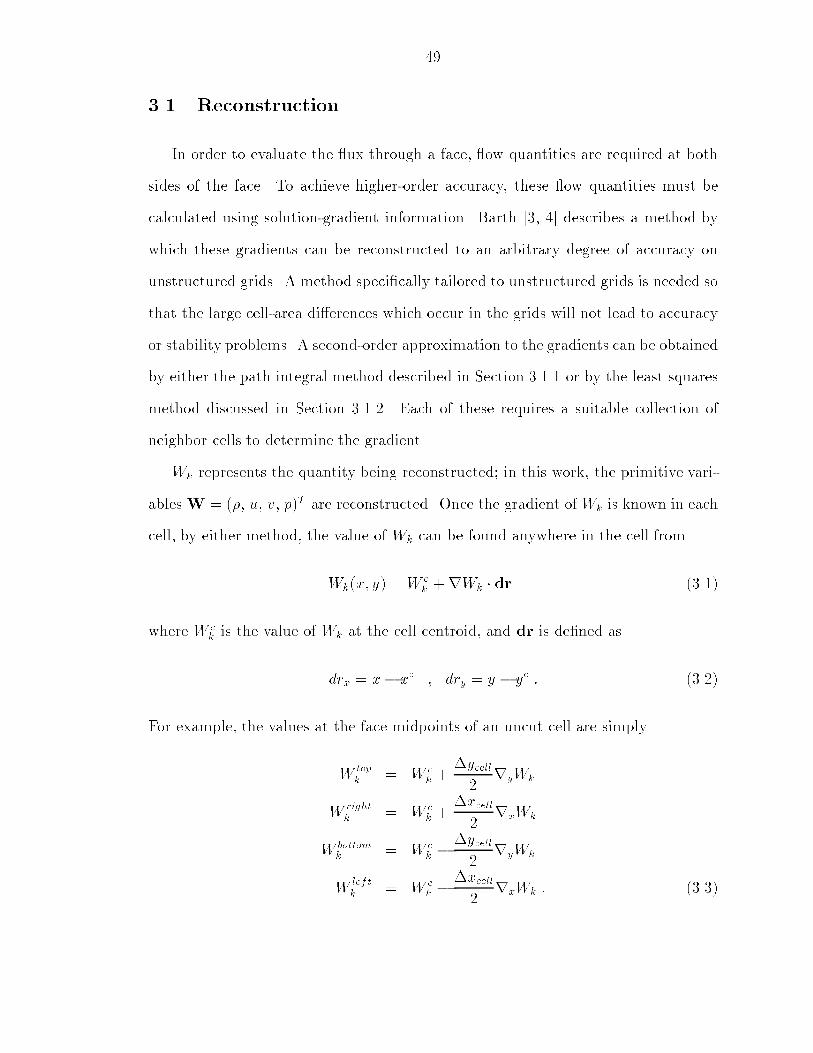
493.1 ReconstructionIn order to evaluate the ux through a face, ow quantities are required at bothsides of the face. To achieve higher-order accuracy, these ow quantities must becalculated using solution-gradient information. Barth [3, 4] describes a method bywhich these gradients can be reconstructed to an arbitrary degree of accuracy onunstructured grids. A method speci�cally tailored to unstructured grids is needed sothat the large cell-area di�erences which occur in the grids will not lead to accuracyor stability problems. A second-order approximation to the gradients can be obtainedby either the path integral method described in Section 3.1.1 or by the least squaresmethod discussed in Section 3.1.2. Each of these requires a suitable collection ofneighbor cells to determine the gradient.Wk represents the quantity being reconstructed; in this work, the primitive vari-ablesW = (�, u, v, p)T are reconstructed. Once the gradient of Wk is known in eachcell, by either method, the value of Wk can be found anywhere in the cell fromWk(x; y) =W ck +rWk � dr (3.1)where W ck is the value of Wk at the cell centroid, and dr is de�ned asdrx = x� xc ; dry = y � yc : (3.2)For example, the values at the face midpoints of an uncut cell are simplyW topk = W ck + �ycell2 ryWkW rightk = W ck + �xcell2 rxWkW bottomk = W ck � �ycell2 ryWkW leftk = W ck � �xcell2 rxWk : (3.3)

50Figure 3.3: \Normal" Path3.1.1 Path IntegralOne option in determining the solution-gradient information relies on a suitablepath integral about the cell of interest. In this option, the gradient of a quantity Wkin a cell is determined by rWk = 1A Z@Wknd` ; (3.4)where A is the area enclosed by the path of integration, @. The path for theintegration is constructed by connecting the centroid of neighboring cells in a counter-clockwise fashion. In most cells, that path is determined by �nding the nearestneighbor in each of eight directions (northwest, west, southwest, south, southeast,east, northeast, north). This \normal" path is depicted in Figure 3.3.An \altered" path is needed for a variety of special geometric con�gurations.These cases fall into one or both of two general categories. The �rst occurs when aneighbor in one of the eight directions has children. Here, the appropriate childrenof the neighbor are used in the path. The second occurs when a neighbor is not avalid cell due to a body or outer boundary. Then, the cell itself is used in the pathinstead of that neighbor. Near a body, as few as four cells may be included in thepath, including the cell itself. Some examples of these \altered" paths are shown inFigure 3.4.

51

Figure 3.4: \Altered" Paths

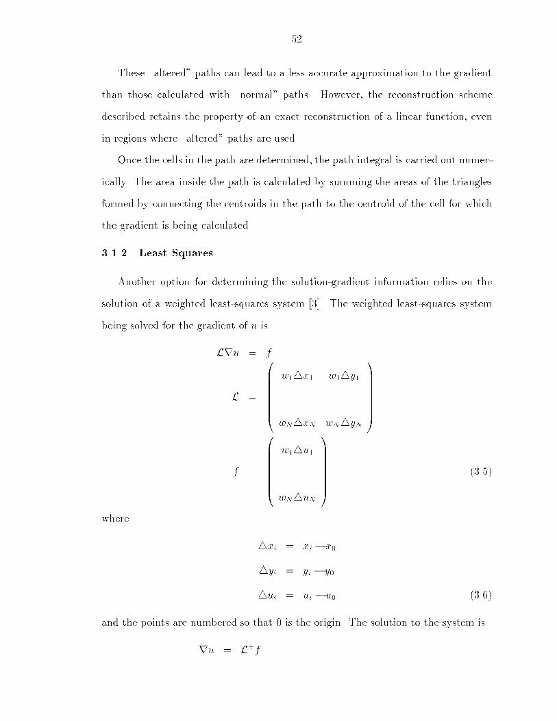
52These \altered" paths can lead to a less accurate approximation to the gradientthan those calculated with \normal" paths. However, the reconstruction schemedescribed retains the property of an exact reconstruction of a linear function, evenin regions where \altered" paths are used.Once the cells in the path are determined, the path integral is carried out numer-ically. The area inside the path is calculated by summing the areas of the trianglesformed by connecting the centroids in the path to the centroid of the cell for whichthe gradient is being calculated.3.1.2 Least SquaresAnother option for determining the solution-gradient information relies on thesolution of a weighted least-squares system [3]. The weighted least-squares systembeing solved for the gradient of u isLru = fL = 0BBBBBBB@ w14x1 w14y1... ...wN4xN wN4yN 1CCCCCCCAf = 0BBBBBBB@ w14u1...wN4uN 1CCCCCCCA (3.5)where 4xi = xi � x04yi = yi � y04ui = ui � u0 (3.6)and the points are numbered so that 0 is the origin. The solution to the system isru = L+f

53L+ = 14 0BB@ LT1 �LT2L2��LT2 �LT1L2�LT2 �LT1L1��LT1 �LT1L2� 1CCA (3.7)where L1 and L2 are the �rst and second columns, respectively, of L and4 = �LT1L1� �LT2L2�� �LT1L2�2 : (3.8)To solve for the gradient of Wk for N neighbors, Equation 3.7 is expanded andsplit into X and Y components asrxWk = 1c1c3 � c22! NXi=1 �w2i [c3 (xi � x0) � c2 (yi � y0)]�W ik �W 0k ��ryWk = 1c1c3 � c22! NXi=1 �w2i [c1 (yi � y0)� c2 (xi � x0)]�W ik �W 0k �� : (3.9)where c1, c2, and c3 are de�ned asc1 = �LT1L1� = PNi=1 �w2i (xi � x0)2�c2 = �LT1L2� = PNi=1 (w2i (xi � x0) (yi � y0))c3 = �LT1L1� = PNi=1 �w2i (yi � y0)2� (3.10)In the above formulas, x0, y0, and W 0k denote the cell about which the gradientrWk is computed. The weights wi provide an added degree of freedom, allowing theenforcement of, for example, an upwind bias in the gradient. For the calculations inthis thesis, however, the weights were all set to one.This gradient calculation requires a cloud of neighboring cells. These cells do notneed to be in any particular order. For simplicity, the cloud was made up of thesame neighbors used in the path for the Path Integral Method. A sample numberingof an \altered" con�guration is shown in Figure 3.5.There is no appreciable di�erence between the results of the two gradient calcula-tion schemes. To show this, gradients were calculated from exact cell-centered valuesand used to create approximate values at the cell corners. The exact value of the

541 2 3

4

5

678

9

10Figure 3.5: Sample Numberingfunction f (x; y) = 2 + cos (�x) + cos (�y). was given to each cell in the grid. Then,cell gradients of this function were computed and cell corner values created from thegradients. The error was then computed between the value computed and the cellcorners and the known exact value. This process was applied to a sequence of �neruniform grids to compare the error to the grid size. Figure 3.6 gives a log-log plot ofgrid spacing versus the L2 norm of the error. The slope of each method asymptotesto two, as it should for second order accuracy. The limited cases begin with lowererrors, but as the grid spacing decreases, all the errors converge to a single value.The limiting procedure is outlined in Section 3.1.3. The path integral method wasused for all cases presented in this dissertation.3.1.3 LimitingIf the full gradient were used in reconstructing the values at face midpoints, thesecomputed values could fall outside the bounds of the values given, for example thoseused to compute the gradient. To avoid this, the computed gradients of the cell arelimited; that is the primitive variables W = (�; u; v; p)T are reconstructed viaW(x; y) =Wc + �rW � dr (3.11)where � is a limiter, with a value between zero and one. In regions where � = 1,the reconstruction used is linear, and the truncation error is O(h2); in regions where

55�1:2 �1:0 �0:8 �0:6�2:2�1:8�1:4�1:0

log10 (4h)log10 (L2) Gradients of f (x; y) = 2 + cos (�x) + cos (�y). Least SquaresLeast Squares with LimitingPath IntegralPath Integral with LimitingFigure 3.6: Grid Spacing vs. Gradient Errors� = 0, the reconstruction used is piecewise constant, and the truncation error isO(h) [3].The limiter used is a di�usive limiter of the minmod variety [53], and is de�nedas � = min8>>>>>>><>>>>>>>: 1mink �jW ck�maxpath(Wk)jjW ck�maxcell(Wk)j �mink �jW ck�minpath(Wk)jjW ck�mincell(Wk)j � : (3.12)The minimum and maximum over the path are found by examining the values of Wkused to compute the gradient; the minimum and maximum over the cell are foundby using the gradient to reconstruct Wk at the corners of the cell. Thus, the limiteracts to ensure that the values of Wk at the nodes of the cell for which the gradientis being calculated are bounded by the values of Wk that are used in calculating thegradient. This limiting procedure is slightly modi�ed for cut cells. For cut cells, theminimum and maximum over the cell is found using the values at the corners of thecell, excluding those on the body. If the values on the body were included in the

56maximum over the cell, the scheme would tend to revert to �rst order in the cellson the body. In standard MUSCL-type schemes [60], a separate limiter is typicallyused for each variable, and for each grid direction, resulting in eight limiters for eachcell. However, using a single limiter for the gradient of the vector W was found togive superior convergence.Unfortunately, limiting can seriously hamper the convergence to a steady state,with the nonlinearity of the scheme resulting in limit cycles. The limiter values insmooth regions of the ow can oscillate. To combat this problem, the limiter valuesare \frozen" after a certain point in the convergence, using previously stored valuesof the limiter rather than recomputing them at each time step. Freezing the limitersallows the residuals to converge to machine zero. Even though the limiter is \frozen",the values of density and pressure are still checked to be sure that they do not dipbelow zero. If they do, a more restrictive limiter is used for the cell for that onetime-step.A new alternative to limiter freezing was recently proposed by Venkatakrish-nan [63]. The limiter in Equation 3.12 is modi�ed to be more like the Van Albadalimiter [53]. This new limiter prevents the limiter from acting in smooth regions ofthe ow, thus allowing the solution to converge. This limiter is, however, a littlemore di�usive, allowing some smearing of the solution near shocks. Also, a tuningvalue is needed to tell the limiter how strictly to enforce limiting.Typical values of the limiter, �(x; y), are shown for a transonic airfoil case. Fig-ure 3.7 gives the Mach contours for this case and Figure 3.8 shows the limiter �. Ascan be seen, a linear reconstruction (� = 1) is used nearly everywhere. In the imme-diate vicinity of the shocks and the wake, the limiter reduces the order of accuracy ofthe scheme. However, the percentage of cells in which the limiter is less than one isextremely small. The limiter values on the body are one, allowing the full accuracyof the scheme there. This is true even for the smallest cut cells.

57�1:50 �0:50 0:50 1:50�1:50�0:500:501:50

XY Mach Contours | Transonic Airfoil Fmin 0.029Fst 0.040Finc 0.040Fmax 1.440Figure 3.7: Mach Contours | Transonic Airfoil

�1:50 �0:50 0:50 1:50�1:50�0:500:501:50 Cell values of the limiter, �Fmin 0.000.050.100.150.200.250.300.350.400.450.500.550.600.650.700.750.800.850.900.95Fmax 1.00

Figure 3.8: Limiter Values | Transonic Airfoil

583.2 Flux FormulationThe ux formulation described here corresponds to the solution of the Eulerequations in two dimensions. An update to a cell is provided by the summation ofthe uxes on the faces making up the cell. After describing the Euler equations in theproper form, two possible methods to compute the ux function will be examined.The �rst method is Roe's Approximate Riemann Solver and second is Van Leer's FluxVector Splitting. In this code, the former was used for most of the cases considered.3.2.1 Euler EquationsThe �nite-volume form of the Euler equations in two dimensions can be writtenas dUdt = � 1A Xfaces (F�y �G�x) (3.13)where A is the area of the cell, �x and �y are the changes of x and y along a face(de�ned so that the integral is carried out in a counter-clockwise direction), and U,F and G are de�ned as U = 0BBBBBBBBBBB@ ��u�v�E 1CCCCCCCCCCCAF = 0BBBBBBBBBBB@ �u�u2 + p�uv�uH 1CCCCCCCCCCCA

59G = 0BBBBBBBBBBB@ �v�vu�v2 + p�vH 1CCCCCCCCCCCA (3.14)where � is the density, u and v are the components of velocity in the x and ydirections, E is the speci�c total energy, and H = E+ p� is the speci�c total enthalpy.De�ning the face length and the normal and tangential velocities as�s = q(�x)2 + (�y)2 (3.15)and un = (u�y � v�x)�sut = (u�x+ v�y)�s ; (3.16)the ux through a face may be written as(F�y �G�x) = 0BBBBBBBBBBB@ �un�unu+ p�y�s�unv � p�x�s�unH 1CCCCCCCCCCCA�s � ��s : (3.17)The function� is a formulation of the ux through a face based on the reconstructionof ow quantities to the \left" and \right" side of the face.For each cell, the face uxes � are summed to give the residual for the cell,Res (U) = � Xfaces� �s : (3.18)These residuals are then integrated in time, as described in section 3.3.For axisymmetric ow, the two dimensional Euler equations must include a sourceterm and can be written asdUdt = � 1A�y Xfaces y (F�y �G�x) + S (3.19)

60with S de�ned as S = 0BBBBBBBBBBB@ 00�p=�y0 1CCCCCCCCCCCA : (3.20)Here, y is the midpoint of the face, �y is the y centroid of the cell, which takes intoaccount that the cell has been rotated about the axis of symmetry, and �p is the cellpressure at the cell centroid. Instead of generating a new function ��, our original� from the two dimensional case can be used. Then equation 3.18 becomesRes (U) = �0@1�y Xfaces y� �s1A+AS : (3.21)With this change, our function � can now be developed in the next sections withoutconsidering the special case of axisymmetric ow.3.2.2 Roe's Flux-Di�erence SplittingThe ux through a face is a function of the values at the face midpoint, givenby the reconstruction in the cells to the \left" and \right" of the face. Using Roe'sapproximate Riemann solver, this ux function � is� (UL;UR) = 12 [� (UL) +� (UR)]� 12 4Xk=1 jakj��VkRk (3.22)with a = 0BBBBBBBBBBB@ un � cununun + c 1CCCCCCCCCCCA

61�V = 0BBBBBBBBBBB@ �p��c�un2c2��utc��� �pc�p+�c�un2c2 1CCCCCCCCCCCAR = 0BBBBBBBBBBB@ 1 0 1 1u� c�y�s c�x�s u u+ c�y�sv + c�x�s c�y�s v v � c�x�sH � unc utc u2+v22 H + unc 1CCCCCCCCCCCA (3.23)and � = p�L�Ru = p�LuL +p�RuRp�L +p�Rv = p�LvL +p�RvRp�L +p�RH = p�LHL +p�RHRp�L +p�R (3.24)where c, un, and ut are calculated directly from �, u, v, and H. The ux di�er-ence terms (the summation in Equation 3.22) provide the upwind character whichstabilizes the scheme.To prevent expansion shocks, an entropy �x is imposed [61]. The entropy control-ling term, ���a(k)���, is replaced by a smoothed value, ���a(k)����, for the two acoustic waves(k = 1, k = 4). For those two waves,���a(k)���� = 8>><>>: ���a(k)��� ���a(k)��� � 12�a(k)(a(k))2�a(k) + 14�a(k) ���a(k)��� � 12�a(k)�a(k) = max �4�a(k); 0� ;�a(k) = a(k)R � a(k)L : (3.25)

623.2.3 Van Leer's Flux SplittingUsing Van Leer's ux vector splitting, the ux function, �, is de�ned as� = T�1 �H+(UL) +H�(UR)� ; (3.26)where T = 0BBBBBBBBBBB@ 1 0 0 00 �y�s ��x�s 00 �x�s �y�s 00 0 0 1 1CCCCCCCCCCCA and H = 0BBBBBBBBBBB@ �un�u2n + p�unut�unH 1CCCCCCCCCCCA : (3.27)The split uxes H+ and H� are de�ned for various normal Mach numbers asMn � 1 H+ = H; H� = 0Mn � �1 H+ = 0; H� = HjMnj � 1 H� = 0BBBBBBBBBBB@ h�1h�2h�3h�4 1CCCCCCCCCCCA = 0BBBBBBBBBBB@ ��c (Mn � 1)2 =4h�1 c [( � 1)Mn � 2] = h�1 cMth�1 c2 �[( � 1)Mn � 2]2 = [2 ( 2 � 1)] +M2t =2� 1CCCCCCCCCCCA :(3.28)3.3 Time SteppingThe time-stepping scheme used is one of the optimally-smoothing multi-stageschemes developed by Tai [54, 62]. A multigrid convergence method is also used toincrease the convergence rate of the solution.3.3.1 Multi-Stage Time SteppingThe general m-stage scheme is de�ned asU(0) = Un

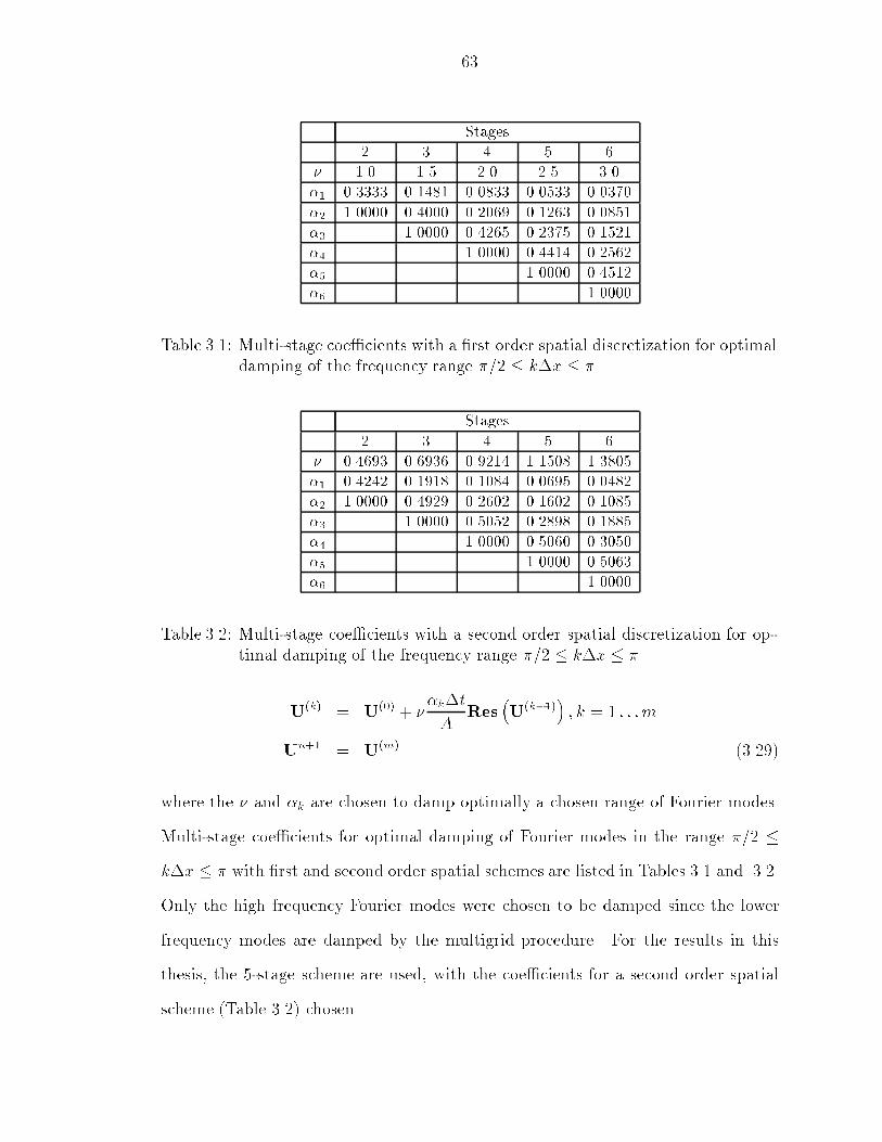
63Stages2 3 4 5 6� 1.0 1.5 2.0 2.5 3.0�1 0.3333 0.1481 0.0833 0.0533 0.0370�2 1.0000 0.4000 0.2069 0.1263 0.0851�3 1.0000 0.4265 0.2375 0.1521�4 1.0000 0.4414 0.2562�5 1.0000 0.4512�6 1.0000Table 3.1: Multi-stage coe�cients with a �rst order spatial discretization for optimaldamping of the frequency range �=2 � k�x � �Stages2 3 4 5 6� 0.4693 0.6936 0.9214 1.1508 1.3805�1 0.4242 0.1918 0.1084 0.0695 0.0482�2 1.0000 0.4929 0.2602 0.1602 0.1085�3 1.0000 0.5052 0.2898 0.1885�4 1.0000 0.5060 0.3050�5 1.0000 0.5063�6 1.0000Table 3.2: Multi-stage coe�cients with a second order spatial discretization for op-timal damping of the frequency range �=2 � k�x � �U(k) = U(0) + ��k�tA Res �U(k�1)� ; k = 1 : : :mUn+1 = U(m) (3.29)where the � and �k are chosen to damp optimally a chosen range of Fourier modes.Multi-stage coe�cients for optimal damping of Fourier modes in the range �=2 �k�x � � with �rst and second order spatial schemes are listed in Tables 3.1 and 3.2.Only the high frequency Fourier modes were chosen to be damped since the lowerfrequency modes are damped by the multigrid procedure. For the results in thisthesis, the 5-stage scheme are used, with the coe�cients for a second order spatialscheme (Table 3.2) chosen.

64Since steady solutions of the Euler equations are computed, local time-steppingis used, and indeed is necessary, since the time-stepping is dependent on the cell size,and the grids generated have extremely large di�erences in area from cell to cell, dueto the cut cells.3.3.2 Multigrid Convergence AccelerationThe improved convergence of multigrid is due in part to the damping of lowfrequency errors on the �ner grids by the use of coarser grids, the parents of the �negrid cells. Because these low frequency errors appear on the coarser grids as highfrequencies, they are e�ciently damped before being sent back to the �ner grids.Another factor in the improved convergence is the fact that waves move farther inone time-step on the coarser grids. Both damping and convection contribute to themultigrid speed-up.Since the Quadtree data structure inherently provides inter-level cell communi-cation, a sequence of multigrid levels can easily be constructed which use the treeto communicate. Thus most of the interface between various multigrid levels hasalready been done. Most multigrid algorithms are applied to a succession of coarseruniform grids. This leaves each cell in the tree with a unique place in the multigridcycle. For this unstructured-grid approach, not only are the cells on the �nest gridnot of the same cell level in the tree, but the cells on subsequent multigrid levelsare not of the same cell level in the tree. This will cause a little complication to themultigrid algorithm, and will eventually lead to implementation of a \saw-tooth"multigrid cycle instead of the more conventional \V" cycle.A cell's level in the tree is de�ned as the number of successive parents to theroot cell. In contrast, the multigrid level is de�ned as the collection of cells usedin a given level of the multigrid algorithm. For M multigrid levels, the cells onmultigrid levelM correspond to the �nest level, including all the computational cells

656 7

4 5

2 3

1

6 7

5

3

4 5

3

2 3 Multigrid

Level 2Multigrid

MultigridLevel 3

Level 1Figure 3.9: 1-Dimensional Multigrid Examplewithout children, i.e. the leaves of the quadtree. If N is the maximum cell level inmultigrid level M . The grid corresponding to multigrid level M � 1 is de�ned as allthe computational cells on cell level N � 1 and all computational cells with a celllevel less than N � 1 having no children. Multigrid level M � 2 down to multigridlevel 1 are constructed similar to level M � 1. It should be noted, however, thatsome cells are included in more than one multigrid level, speci�cally cells withoutchildren which are at a cell level less than N . To visualize what is happening here,a one-dimensional case is given in Figure 3.9. The one-dimensional grid is drawn sothat the coarser parent cells can be seen. If cell 1 is the root cell, then the maximumcell level in the tree, N , is three. If three multigrid levels, M , are used, cell number5 is used on two multigrid levels and cell number 3 is used on three multigrid levels.Special care will need to be taken in these cells.Since the multigrid algorithm makes use of cells with children, accurate statevalues are needed for these cells. The values for these cells depend on the values oftheir children. The conserved variables are transferred from the children (grid levelL + 1) to the parents (grid level L) by an area weighted collection operator, ILL+1,

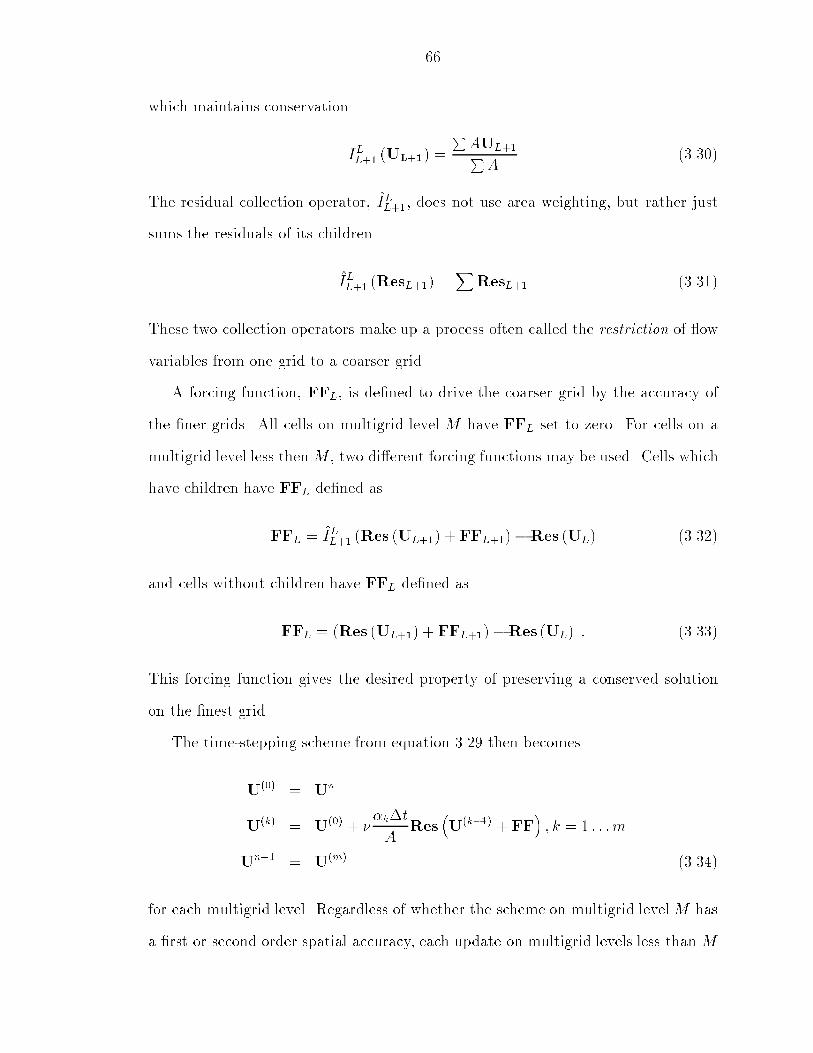
66which maintains conservation.ILL+1 (UL+1) = PAUL+1PA (3.30)The residual collection operator, ILL+1, does not use area weighting, but rather justsums the residuals of its children.ILL+1 (ResL+1) =XResL+1 (3.31)These two collection operators make up a process often called the restriction of owvariables from one grid to a coarser grid.A forcing function, FFL, is de�ned to drive the coarser grid by the accuracy ofthe �ner grids. All cells on multigrid level M have FFL set to zero. For cells on amultigrid level less then M , two di�erent forcing functions may be used. Cells whichhave children have FFL de�ned asFFL = ILL+1 (Res (UL+1) + FFL+1)�Res (UL) (3.32)and cells without children have FFL de�ned asFFL = (Res (UL+1) + FFL+1)�Res (UL) : (3.33)This forcing function gives the desired property of preserving a conserved solutionon the �nest grid.The time-stepping scheme from equation 3.29 then becomesU(0) = UnU(k) = U(0) + ��k�tA Res�U(k�1) + FF� ; k = 1 : : :mUn+1 = U(m) (3.34)for each multigrid level. Regardless of whether the scheme on multigrid levelM hasa �rst or second order spatial accuracy, each update on multigrid levels less than M

67Update U

Create FFUpdate U

Restrict U

Create FFUpdate U

Restrict U

Create FFUpdate U

Restrict U Prolong dU

Prolong dU

Prolong dU

4=M

LevelMultigrid

3

2

1 Figure 3.10: Multigrid Saw-Tooth Cycleuses a �rst order spatial operator (ie no linear reconstruction). This allows a greatersmoothing of the high frequency errors on the coarser grid while still maintaining theaccuracy on the �ne grid. Once the coarse grid state vectors, U, have been updated,the corrections need to be sent back to the �ner grids. The correction to UL+1 isde�ned as Un+1L+1 = Un+1L+1 +r �Un+1L �UnL� � dr (3.35)where the gradient of the di�erence Un+1L � UnL is computed in the same way thatthe gradients of the state vector are computed, a path integral reconstruction. Thiscorrection process is often referred to as the prolongation of the the error correction.The multigrid algorithm constructed from these operators is depicted in Fig-ure 3.10. The multigrid algorithm begins by updating UM on multigrid level M(Equation 3.29). Then on multigrid level M � 1, accurate state values, UM�1, arecreated (Equation 3.30), the forcing function, FFM�1, is computed (Equation 3.31),and UM�1 updated in time (Equation 3.34). This process proceeds by level downto multigrid level 1. When multigrid level 1 is reached, the correction is sent to

68the state vector, U, up to multigrid level 2 (Equation 3.35). At this point eithera \saw-tooth" or \V" cycle must be chosen. The saw-tooth procedure dictates justpassing the correction level by level back to multigrid level M , or the �nest grid,before starting the procedure over (again Equation 3.35). On the other hand, theV cycle requires that U be updated in time (Equation 3.34) before the correctionis passed up to the next level. However, the update requires knowing the forcingfunction used for that cell on the way down. This can be seen by again examiningFigure 3.9. Cell number 3 is used in three di�erent multigrid levels. The forcingfunction on multigrid level 3 is zero, but the forcing functions on multigrid levels2 and 3 are not zero, and are unique values. Two di�erent forcing functions needto be stored. It is common in many cases for a few cells to be used on all of themultigrid levels, requiring a di�erent forcing function on each level. Storing eachof these forcing functions can lead to a huge increase in the storage needs of themultigrid algorithm. The V cycle uses the forcing function for each cell twice, oncein the restriction stage and once in the prolongation stage. However, a saw-toothcycle only uses the forcing function in the restriction stage. When a cell is includedin two multigrid levels, the �rst forcing function for the cell is computed normally.When the next multigrid level needs to create a forcing function for that cell, thevalue already stored is used in computing the next value, which will be stored inits place. Thus, by using a saw-tooth multigrid algorithm, no increase in storage isneeded for these special case cells. This choice does not, however, mean that theconvergence acceleration of the multigrid algorithm is substantially reduced, sincethe V cycle requires more work to compute. A comparison of saw-tooth and V cycleresults is included in the multigrid validation study, Section 3.6.3. The saw-toothmultigrid method was implemented for the cases in this thesis.

693.4 Boundary ProceduresThere are two kinds of boundary conditions which must be implemented, froma data structure point of view. The �rst is the \far-�eld" boundary condition. The ow solver needs to know how to handle ow through the outer domain of a ow�eldwhen no body exists on that boundary. The second type of boundary condition isneeded for cells which are cut by a body. The types of conditions which can be setare very similar for each of these, although the implementation is quite di�erent.3.4.1 Far-Field Boundary ConditionsThe computational domain is surrounded by a ring of \ghost" cells used to im-plement the far-�eld boundary conditions. The generation of these ghost cells andhow they relate to the computational cells was discussed in Section 2.2. The statevalues stored in the ghost cells may or may not be used at all, depending on thetype of boundary condition imposed there. Note that ghost cells are not used in thegradient calculation for cells just inside the computational ow �eld. The gradientcalculation is the same no matter what type of boundary condition exists, either inthe far-�eld or on the body.A number of types of far-�eld boundary conditions can be implemented. The mostcommon is simply imposing a freestream condition which completely surrounds the ow. A more general variety of this requires specifying a function of x and y in theghost cells. When a computational cell on the outer boundary requires a ux for theface on the outer boundary, the outside state is speci�ed by the state in the ghostcell neighbor. The grid smoothing routine makes sure that the cell level of ghost cellswill always equal the cell level of its neighbor in the computational ow. Thus thefunction representing the outer boundary condition is given to the resolution of thegrid at that point. The boundary conditions may also change with time. The valuesstored in the ghost cells can be updated each iteration.

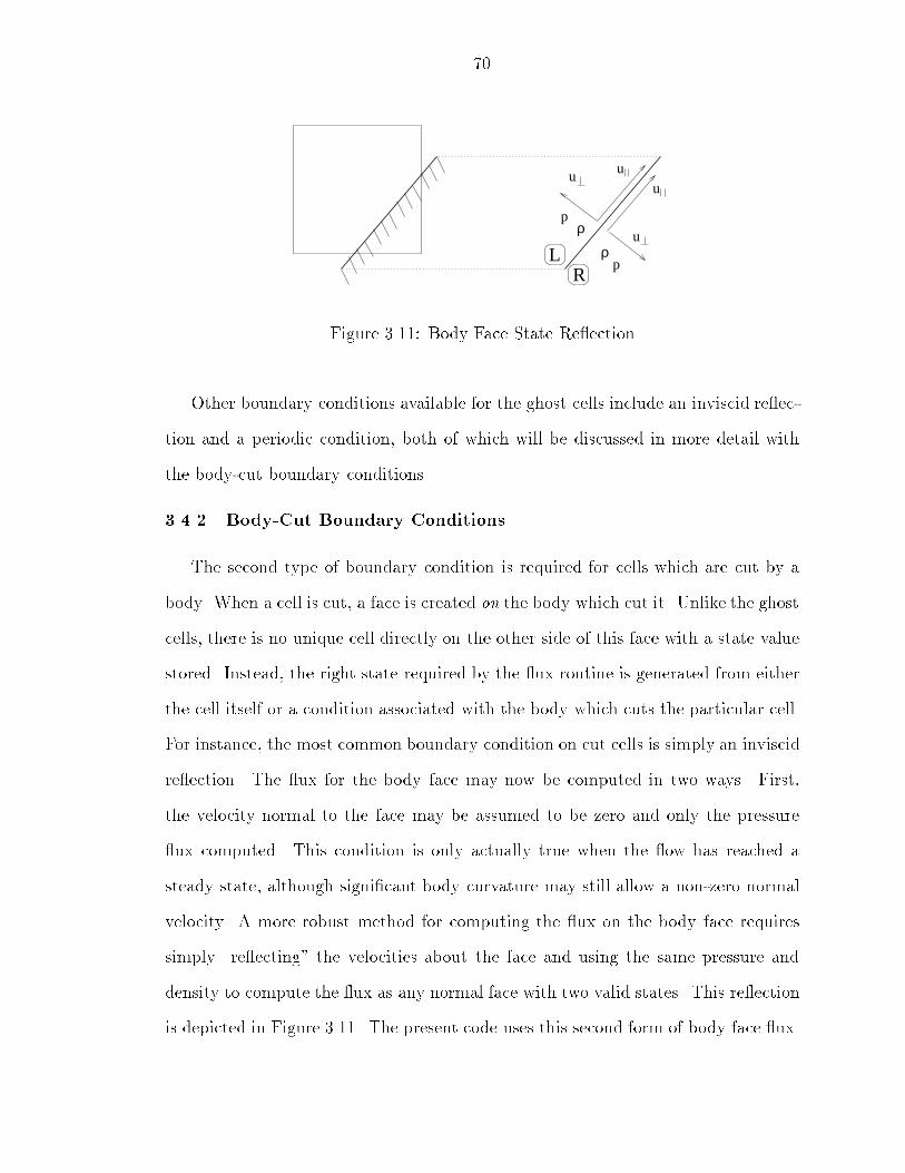
70u u

u

uρ

p

ρp

RLFigure 3.11: Body Face State Re ectionOther boundary conditions available for the ghost cells include an inviscid re ec-tion and a periodic condition, both of which will be discussed in more detail withthe body-cut boundary conditions.3.4.2 Body-Cut Boundary ConditionsThe second type of boundary condition is required for cells which are cut by abody. When a cell is cut, a face is created on the body which cut it. Unlike the ghostcells, there is no unique cell directly on the other side of this face with a state valuestored. Instead, the right state required by the ux routine is generated from eitherthe cell itself or a condition associated with the body which cuts the particular cell.For instance, the most common boundary condition on cut cells is simply an inviscidre ection. The ux for the body face may now be computed in two ways. First,the velocity normal to the face may be assumed to be zero and only the pressure ux computed. This condition is only actually true when the ow has reached asteady state, although signi�cant body curvature may still allow a non-zero normalvelocity. A more robust method for computing the ux on the body face requiressimply \re ecting" the velocities about the face and using the same pressure anddensity to compute the ux as any normal face with two valid states. This re ectionis depicted in Figure 3.11. The present code uses this second form of body face ux.

71The body face may also have a �xed right state similar to the outer boundarycondition. The di�erence is that the value used is stored with the body which cutsthe cell. Each body may have a di�erent type of boundary condition associated withit. If di�erent conditions are needed for a single body, the body can be made up ofany number of sub-bodies, each with its own boundary condition. For example, thiscondition is useful for mass injection through a surface.A �nal variety of boundary condition is the periodic condition. Here a period isspeci�ed by a change in the X and/or Y directions. Then, when the right state isrequired for a body face, the x and y o�sets are added to the face midpoint, the cellcontaining this point is found, and the right state is computed. In general, the cellcontaining this o�set point will be found on a body identical to the �rst, only o�setby the period. Cases may be constructed in which this is not true however. Theonly requirement is that the o�set point be found within a valid computational cell.Figure 3.12 gives a simple example.3.5 Post-ProcessingPost-processing requires transferring the known cell-centered values to nodal val-ues for plotting as accurately as possible. The same limited cell gradients used in the ow solver are used to extrapolate to each cell's nodes as shown in Figure 3.13. Thefunction as reconstructed at the nodes is multivalued; there is one value resultingfrom the representation in each cell sharing that node. Also, nodes on a re ectingbody may have the re ection of the sent value as well. These multiple values ateach node are averaged to yield a single accurate, bounded value. This yields a statevector at each node, allowing any desired quantity to be computed and used forplotting.

72UR

ULFigure 3.12: Example of Periodic Boundary Condition

Figure 3.13: Obtaining Post-Processed Nodal Values

733.6 ValidationIn order to validate the method described in this thesis, a careful examinationof the convergence and accuracy will be given. First, the convergence accelerationof multigrid will be examined, along with comparisons of the saw-tooth and V cyclealgorithms. Then the accuracy of some special boundary conditions will be given.Finally, a detailed order of accuracy study will show that the scheme is second orderaccurate, and that the magnitude of the error is acceptable.3.6.1 Small Cut CellsA common problem with Cartesian grid methods is that very small cells canexist in the grid due to the somewhat arbitrary way that the grid intersects thebody. In fact, cells are commonly found at an area on the order of 10�4 times thatof a neighboring uncut cell. Since the code is designed for steady-state solutions,local time-stepping may be used to remove the sti�ness due to these small cells.A di�erence in time-steps is not the only issue raised by the small cells, however.Depending on the spatial discretization used in the update schemes, the values inthe small cells can decouple from those in their neighbors, leading to \spikes" in theresults in the vicinity of the small cells. Even with very sophisticated schemes, suchas that proposed by LeVeque [8], cells smaller in area than 1% of that of a neighborcan lead to problems. The solution to this problem adopted in this work is to usea spatial discretization suited to unstructured grids, speci�cally the reconstructionapproach of Barth [3]. This combination of the gradient reconstruction and the localtime-stepping allowed the solutions to converge as accurately as if the small cells didnot exist. Although this work consists primarily of steady ow cases, if unsteadycases need study, a uniform time stepping could be used with some type of cellmerging to allow the solution to converge in a reasonable time [5].

743.6.2 Multigrid Grid ProblemsA troubling grid feature which leads to some di�culty is the existence of cellswhich would violate the data structure, speci�cally cells which are cut more thanonce. A description of these cells is given in the write-up of the smoothing procedurein Section 2.5. The grid smoothing removes the feature from the �nest grid. However,multigrid makes use of the parents of these cells in creating a coarser grid to dampout the low frequency errors. In order to make use of the multigrid convergenceacceleration for geometries with this grid problem, a \cone of in uence" approachwas used around these bad cells. First, each cell on the direct parental successionfrom the original problem cell to the root was agged as a problem cell. Then anyneighbor to one of these problem cells is handled in a special way when a multigridupdate is needed for that cell. Speci�cally, these cells receive an accurate restrictionof state values from their children, but they are not advanced in time. This is becauseno state value is available one of the cell's neighbors, thus no ux can be computedon the face shared with that neighbor.These cells handled specially make up the \cone of in uence" of the originalproblem cell. Figure 3.14 gives an example of such a grid. Part (a) of this �gureshows a portion of a grid and data tree in which one cell violates the data structure.Smoothing of the grid results in the grid and data tree given in part (b). Part (c)again gives the data tree, but with each problem cell and \cone of in uence" cellidenti�ed. Note that no cells without children are agged. This process only a�ectsthe coarser grids used for multigrid.3.6.3 Multigrid Convergence StudyIn examining the convergence acceleration bene�ts of the multigrid algorithm, it is�rst important to determine the di�erences in convergence characteristics between asaw-tooth and V cycle algorithm. When that is completed, the multigrid convergence

75

Cone Of Influence Cells

Problem Cells

(a)

(b)

(c)

Figure 3.14: Multigrid Cone of In uence

760: 100: 200: 300:�8:�5:�2:1:

Number of Cycleslog10 (Res) NACA 0012 at M = 0:2 and � = 0No MultigridSaw-Tooth CycleV CycleFigure 3.15: Subsonic Convergence History Based on Multigrid Cyclescan be studied in greater detail.To see how the saw-tooth and V cycles compare, a NACA 0012 airfoil was runat both subsonic (M = 0:2 and � = 0) and transonic (M = 0:85 and � = 1) speedsusing �ve multigrid levels. Figure 3.15 shows the convergence history for the subsoniccase. The plot includes convergence for: a 5-stage V cycle, a 5-stage saw-tooth cycle,and no multigrid. The V cycle shows a slightly better convergence rate than thesaw-tooth cycle. However, since the V cycle is doing more work, it is not a faircomparison. The convergence history based on the number of residual calculations isplotted in Figure 3.16. Here, the saw-tooth cycle actually has a better convergencerate.Figure 3.17 shows the convergence history for the transonic case. The plot in-cludes convergence for: a 5-stage V cycle, a 5-stage saw-tooth cycle, and no multigrid.The V cycle shows a slightly better convergence rate than the saw-tooth method baseson cycles. But when convergence is based on the number of residual calculations,the saw-tooth cycle actually has a better convergence rate, given in Figure 3.18.

770: 2x106 4x106 6x106�8:�5:�2:1:

Number of Residual Calculationslog10 (Res) NACA 0012 at M = 0:2 and � = 0No MultigridSaw-Tooth CycleV CycleFigure 3.16: Subsonic Convergence History Based on Residual Calculations

0: 100: 200: 300:�8:�5:�2:1:Number of Cycles

log10 (Res) NACA 0012 at M = 0:85 and � = 1Saw-Tooth CycleV Cycle No Multigrid

Figure 3.17: Transonic Convergence History Based on Multigrid Cycles

780: 2x106 4x106 6x106�8:�5:�2:1:

Number of Residual Calculationslog10 (Res) NACA 0012 at M = 0:85 and � = 1

Saw-Tooth CycleV Cycle No MultigridFigure 3.18: Transonic Convergence History Based on Residual CalculationsNot all cases will necessarily converge more quickly with a saw-tooth cycle, but itis at the least very near to the convergence of a more conventional V cycle. Becausethe saw-tooth cycle is also much more memory e�cient to implement in this code, asaw-tooth multigrid cycle will be used for the rest of the thesis.An important variable yet to be determined is the number of multigrid levels touse. Any number can be used, provided that many cell levels in the tree exist. Atsome point the improvement in convergence becomes negligible and the extra workrequired hurts the time to converge a solution. To see how the number of multigridlevels a�ect convergence, a NACA 0012 airfoil at M = 0:85 and � = 1 was run usingbetween one and seven multigrid levels. Figure 3.19 shows the convergence historybased on the number of multigrid cycles.As can be seen, the convergence rates are nearly identical for �ve through sevenmultigrid levels. But, since the work required increases with the number of multigridlevels, the solutions will require increasing amounts of time. The convergence historybased on the number of residual calculations is plotted in Figure 3.20. Note that

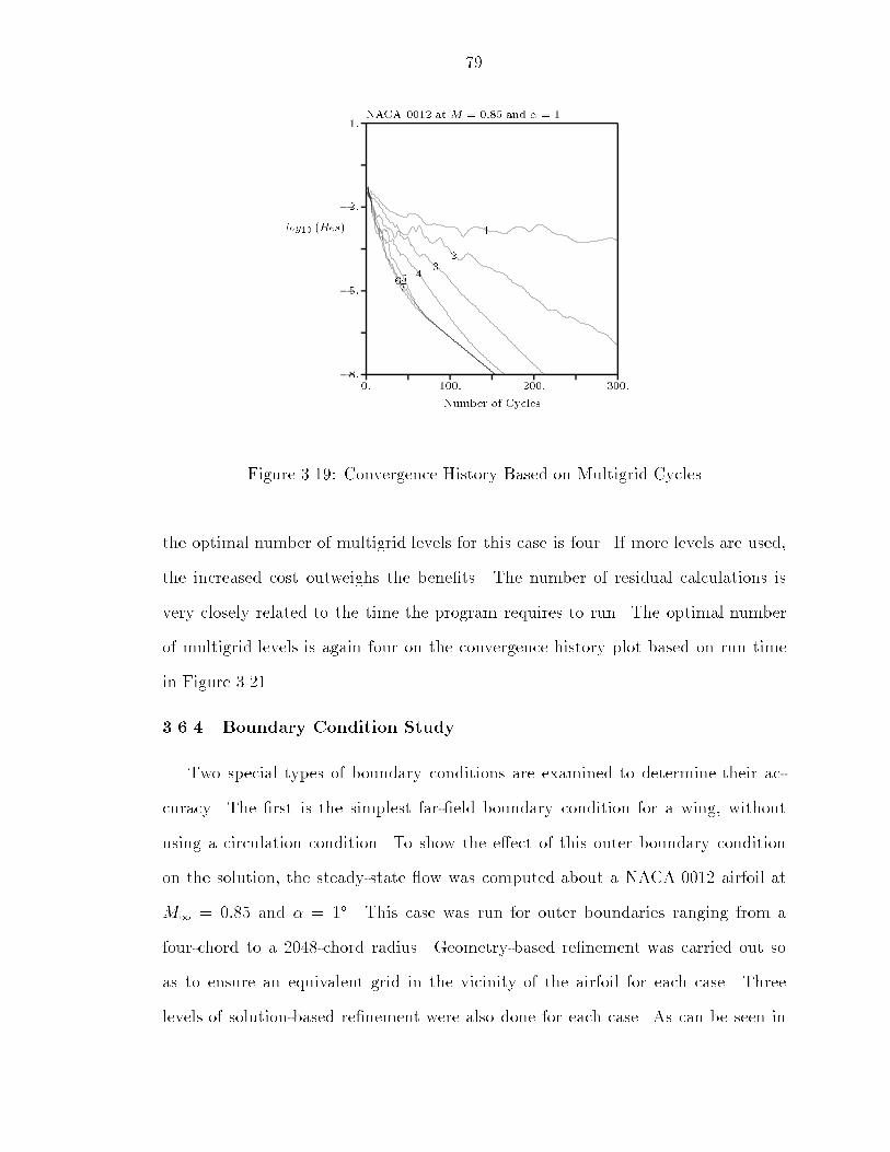
790: 100: 200: 300:�8:�5:�2:1:

Number of Cycleslog10 (Res) NACA 0012 at M = 0:85 and � = 11234567

Figure 3.19: Convergence History Based on Multigrid Cyclesthe optimal number of multigrid levels for this case is four. If more levels are used,the increased cost outweighs the bene�ts. The number of residual calculations isvery closely related to the time the program requires to run. The optimal numberof multigrid levels is again four on the convergence history plot based on run timein Figure 3.21.3.6.4 Boundary Condition StudyTwo special types of boundary conditions are examined to determine their ac-curacy. The �rst is the simplest far-�eld boundary condition for a wing, withoutusing a circulation condition. To show the e�ect of this outer boundary conditionon the solution, the steady-state ow was computed about a NACA 0012 airfoil atM1 = 0:85 and � = 1�. This case was run for outer boundaries ranging from afour-chord to a 2048-chord radius. Geometry-based re�nement was carried out soas to ensure an equivalent grid in the vicinity of the airfoil for each case. Threelevels of solution-based re�nement were also done for each case. As can be seen in

800: 2x106 4x106 6x106�8:�5:�2:1:

Number of Residual Calculationslog10 (Res) NACA 0012 at M = 0:85 and � = 11234567Figure 3.20: Convergence History Based on Residual Calculations

0: 400: 800: 1200:�8:�5:�2:1:Time (seconds)

log10 (Res) NACA 0012 at M = 0:85 and � = 11234567Figure 3.21: Convergence History Based on Run Time

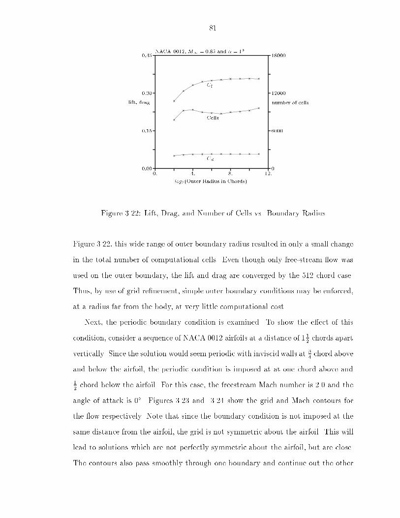
810: 4: 8: 12:0:000:150:300:45

060001200018000log2(Outer Radius in Chords)

lift, drag number of cellsNACA 0012,M1 = 0:85 and � = 1�CdClCells

Figure 3.22: Lift, Drag, and Number of Cells vs. Boundary RadiusFigure 3.22, this wide range of outer boundary radius resulted in only a small changein the total number of computational cells. Even though only free-stream ow wasused on the outer boundary, the lift and drag are converged by the 512 chord case.Thus, by use of grid re�nement, simple outer boundary conditions may be enforced,at a radius far from the body, at very little computational cost.Next, the periodic boundary condition is examined. To show the e�ect of thiscondition, consider a sequence of NACA 0012 airfoils at a distance of 112 chords apartvertically. Since the solution would seem periodic with inviscid walls at 34 chord aboveand below the airfoil, the periodic condition is imposed at at one chord above and12 chord below the airfoil. For this case, the freestream Mach number is 2.0 and theangle of attack is 0�. Figures 3.23 and 3.24 show the grid and Mach contours forthe ow respectively. Note that since the boundary condition is not imposed at thesame distance from the airfoil, the grid is not symmetric about the airfoil. This willlead to solutions which are not perfectly symmetric about the airfoil, but are close.The contours also pass smoothly through one boundary and continue out the other

82�1: 0: 1: 2:�0:50:00:5

1:0X

Y Periodic NACA 0012 Grid PlotFigure 3.23: Grid for Periodic NACA 0012 Caseboundary. A Mach number cross-section plot at y = 0:6 and y = 0:9 is given inFigure 3.25. These two lines both represent a distance of 0.6 chords from the airfoilin each direction. A good agreement is shown, verifying the accuracy of the periodiccondition.3.6.5 Order of Accuracy StudyA careful accuracy assessment study is needed to verify that the ow solutionprocedure described behaves as accurately as expected [13]. To do this, three subsonictest cases have been chosen which will show the accuracy of the scheme and its bodyboundary conditions. These cases will show both the order and the magnitude of theerror.3.6.5.1 Subsonic Non-Lifting AirfoilThe �rst case consists of a NACA 0012 airfoil at M1 = 0:2 and � = 0�. Since the ow remains subsonic throughout, the value of the limiter is likewise one throughout.To examine the overall order of the scheme, this case was run on increasingly �ner

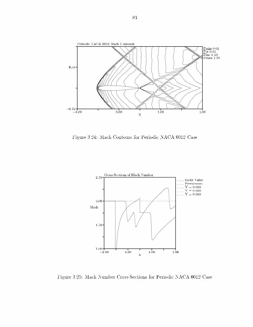
83�1:00 0:00 1:00 2:00�0:500:50 XY Periodic NACA 0012 Mach Contours Fmin 0.01Fst 0.05Finc 0.10Fmax 2.39Figure 3.24: Mach Contours for Periodic NACA 0012 Case

�1:00 0:00 1:00 2:001:001:502:002:50XMach Cross-Sections of Mach Number Body ValueFreestreamY = 0.000Y = 0.600Y = 0.900

Figure 3.25: Mach Number Cross-Sections for Periodic NACA 0012 Case

84�1:75 �1:25 �0:75 �0:25�3:25�2:75�2:25�1:75

Log10 (GridSize)Log10 (Drag)

Figure 3.26: Convergence Rate of Drag as a Function of Grid Sizegrids to examine the e�ect on the drag (which should be zero). Figure 3.26 is alog{log plot of the drag as a function of the size of an uncut cell of the grid. Theslope of this curve, for all but the coarsest grid (which has only eight points on theairfoil), is two, demonstrating the second-order global accuracy of the scheme.3.6.5.2 Subsonic CylinderThe second case which highlights the magnitude of the error is a subsonic cylinderat M1 = 0:38. The lift and drag should both be zero and no entropy should beproduced at all. The lift does remain zero for all grid resolutions, but drag andentropy are non-zero. The entropy contours for the �rst of three grids are shownin Figure 3.27. The grid has a spacing of dh = 0:125. The entropy contours forgrids with dh = 0:0625 and dh = 0:03125 are given in Figures 3.28 and 3.29. Themagnitude of the drag and the maximum entropy drop to an acceptable level forthe �nest grid. This grid has 124 cells on the body, and fewer than this would notnormally be used in practice for a �nal solution. The entropy and drag for the three

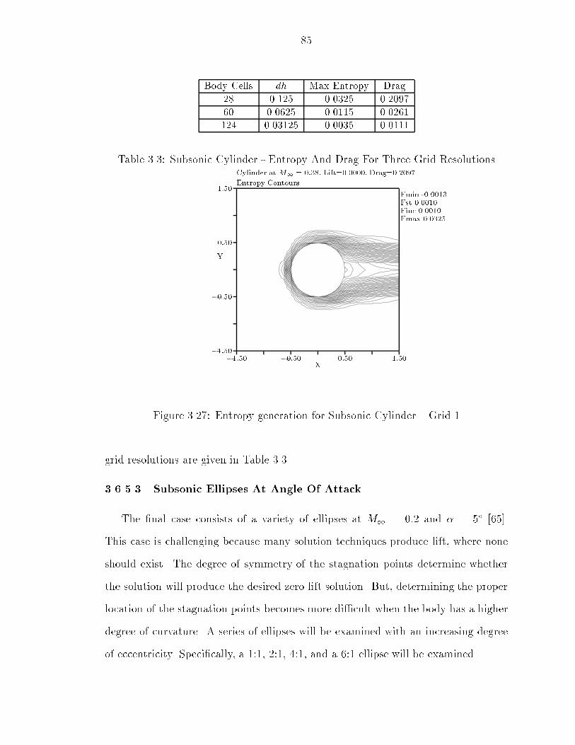
85Body Cells dh Max Entropy Drag28 0.125 0.0325 0.209760 0.0625 0.0115 0.0261124 0.03125 0.0035 0.0111Table 3.3: Subsonic Cylinder - Entropy And Drag For Three Grid Resolutions�1:50 �0:50 0:50 1:50�1:50�0:500:501:50

XY Entropy ContoursCylinder at M1 = 0:38, Lift=0.0000, Drag=0.2097Fmin -0.0013Fst 0.0010Finc 0.0010Fmax 0.0325Figure 3.27: Entropy generation for Subsonic Cylinder { Grid 1grid resolutions are given in Table 3.3.3.6.5.3 Subsonic Ellipses At Angle Of AttackThe �nal case consists of a variety of ellipses at M1 = 0:2 and � = 5� [65].This case is challenging because many solution techniques produce lift, where noneshould exist. The degree of symmetry of the stagnation points determine whetherthe solution will produce the desired zero lift solution. But, determining the properlocation of the stagnation points becomes more di�cult when the body has a higherdegree of curvature. A series of ellipses will be examined with an increasing degreeof eccentricity. Speci�cally, a 1:1, 2:1, 4:1, and a 6:1 ellipse will be examined.

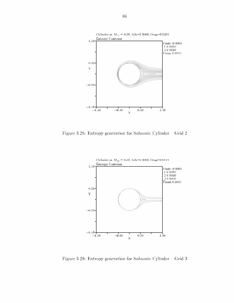
86�1:50 �0:50 0:50 1:50�1:50�0:500:501:50

XY Entropy ContoursCylinder at M1 = 0:38, Lift=0.0000, Drag=0.0261Fmin -0.00041 0.00102 0.0010Fmax 0.0115Figure 3.28: Entropy generation for Subsonic Cylinder { Grid 2

�1:50 �0:50 0:50 1:50�1:50�0:500:501:50XY Entropy ContoursCylinder at M1 = 0:38, Lift=0.0000, Drag=0.01111 0.00102 0.00203 0.0030Fmin -0.0001Fmax 0.0035

Figure 3.29: Entropy generation for Subsonic Cylinder { Grid 3

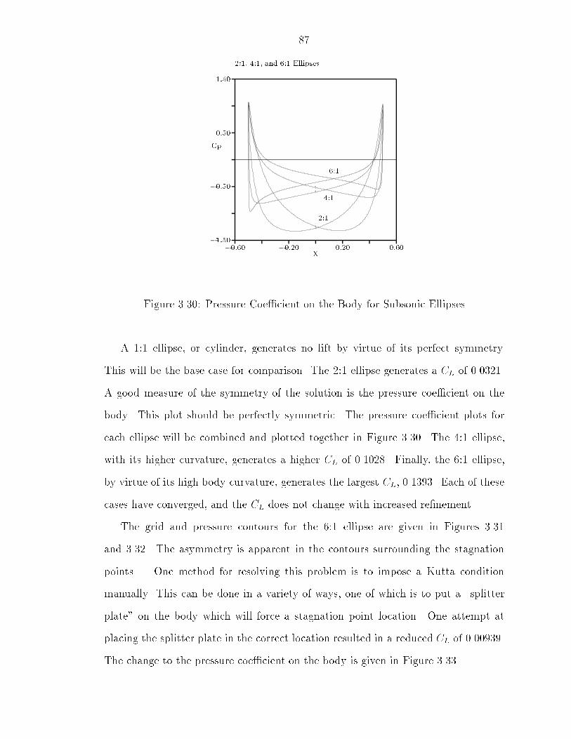
87�0:60 �0:20 0:20 0:60�1:50�0:500:501:50

XCp 2:1, 4:1, and 6:1 Ellipses2:14:16:1Figure 3.30: Pressure Coe�cient on the Body for Subsonic EllipsesA 1:1 ellipse, or cylinder, generates no lift by virtue of its perfect symmetry.This will be the base case for comparison. The 2:1 ellipse generates a CL of 0.0321.A good measure of the symmetry of the solution is the pressure coe�cient on thebody. This plot should be perfectly symmetric. The pressure coe�cient plots foreach ellipse will be combined and plotted together in Figure 3.30. The 4:1 ellipse,with its higher curvature, generates a higher CL of 0.1028. Finally, the 6:1 ellipse,by virtue of its high body curvature, generates the largest CL, 0.1393. Each of thesecases have converged, and the CL does not change with increased re�nement.The grid and pressure contours for the 6:1 ellipse are given in Figures 3.31and 3.32. The asymmetry is apparent in the contours surrounding the stagnationpoints. One method for resolving this problem is to impose a Kutta conditionmanually. This can be done in a variety of ways, one of which is to put a \splitterplate" on the body which will force a stagnation point location. One attempt atplacing the splitter plate in the correct location resulted in a reduced CL of 0.00939.The change to the pressure coe�cient on the body is given in Figure 3.33.

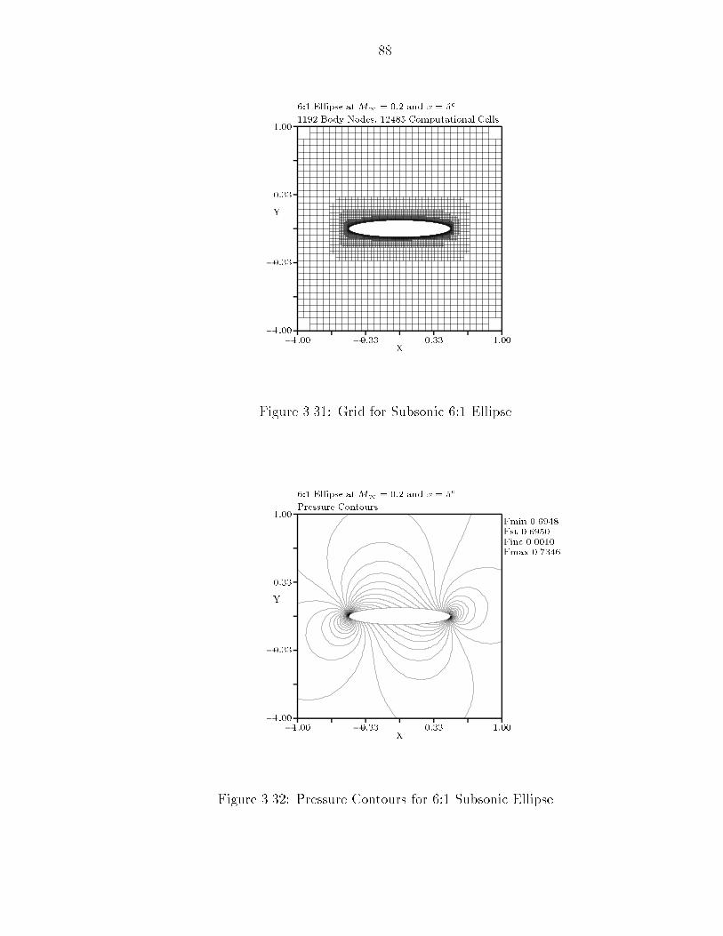
88�1:00 �0:33 0:33 1:00�1:00�0:330:331:00

XY 1192 Body Nodes, 12485 Computational Cells.6:1 Ellipse at M1 = 0:2 and � = 5�Figure 3.31: Grid for Subsonic 6:1 Ellipse

�1:00 �0:33 0:33 1:00�1:00�0:330:331:00XY Pressure Contours6:1 Ellipse at M1 = 0:2 and � = 5� Fmin 0.6948Fst 0.6950Finc 0.0010Fmax 0.7346

Figure 3.32: Pressure Contours for 6:1 Subsonic Ellipse

89

�0:60 �0:20 0:20 0:60�1:50�0:500:501:50XCp 6:1 Ellipse

Figure 3.33: New Pressure Coe�cient on the Body for 6:1 Subsonic Ellipse

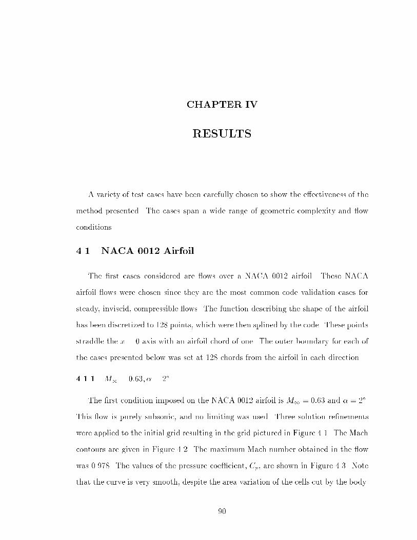
CHAPTER IVRESULTSA variety of test cases have been carefully chosen to show the e�ectiveness of themethod presented. The cases span a wide range of geometric complexity and owconditions.4.1 NACA 0012 AirfoilThe �rst cases considered are ows over a NACA 0012 airfoil. These NACAairfoil ows were chosen since they are the most common code validation cases forsteady, inviscid, compressible ows. The function describing the shape of the airfoilhas been discretized to 128 points, which were then splined by the code. These pointsstraddle the x = 0 axis with an airfoil chord of one. The outer boundary for each ofthe cases presented below was set at 128 chords from the airfoil in each direction.4.1.1 M1 = 0:63; � = 2�The �rst condition imposed on the NACA 0012 airfoil is M1 = 0:63 and � = 2�.This ow is purely subsonic, and no limiting was used. Three solution re�nementswere applied to the initial grid resulting in the grid pictured in Figure 4.1. The Machcontours are given in Figure 4.2. The maximum Mach number obtained in the owwas 0.978. The values of the pressure coe�cient, Cp, are shown in Figure 4.3. Notethat the curve is very smooth, despite the area variation of the cells cut by the body.90

91�1:50 �0:50 0:50 1:50�1:50�0:500:501:50

XY 494 Body Nodes, 10694 Computational Cells.NACA 0012 at M1 = 0:63 and � = 2�Figure 4.1: Grid for NACA 0012 at M1 = 0:63; � = 2�This ow solution has 494 nodes on the body and a resulting lift, CL, of 0.3289 anda drag, CD, of 0.0004. This grid has 10694 cells, so an equivalent structured gridwould be 494 by 21 with the same number of cells on the body, or more realistically,146 by 73. A good structured grid solution produced a CL of 0.3335, and a CD of0.00003 for a 257 by 65 grid [56]. Contours of total pressure loss, 1 � p0=p1, aregiven in Figure 4.4, with the values on the body given in Figure 4.5.4.1.2 M1 = 0:85; � = 1Next the ow solution is obtained for a NACA 0012 at M1 = 0:85 and � = 1�.For these conditions, shocks of comparable strength exist on the upper and lowersurfaces of the airfoil, with a shear layer emanating from the trailing edge. Fivesolution adaptation steps were taken. The grid and Mach contours for this caseare pictured in Figures 4.6 and 4.7. The shocks are both well resolved and a crispshear layer is computed. It should be noted that the contours pass smoothly throughgrid level changes; neither the ow solver nor the post-processing procedure causes

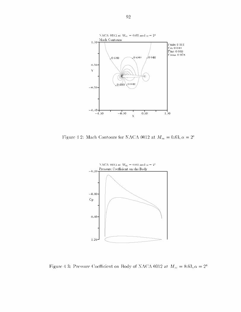
92�1:50 �0:50 0:50 1:50�1:50�0:500:501:50

XY Mach ContoursNACA 0012 at M1 = 0:63 and � = 2�0.680 0.6400.6400.600 0.640 Fmin 0.011Fst 0.040Finc 0.040Fmax 0.978Figure 4.2: Mach Contours for NACA 0012 at M1 = 0:63; � = 2�

1:200:40�0:40�1:20Cp Pressure Coe�cient on the BodyNACA 0012 at M1 = 0:63 and � = 2�Figure 4.3: Pressure Coe�cient on Body of NACA 0012 at M1 = 0:63; � = 2�

93�1:50 �0:50 0:50 1:50�1:50�0:500:501:50

XY 1� p0=p1 ContoursNACA 0012 at M1 = 0:63 and � = 2� Fmin -0.0041Fst 0.0010Finc 0.0010Fmax 0.0208Figure 4.4: 1 � p0=p1 Contours for NACA 0012 at M1 = 0:63; � = 2�

�0:0100:0100:0300:0501� p0=p1 1� p0=p1 on the BodyNACA 0012 at M1 = 0:63 and � = 2�Figure 4.5: 1 � p0=p1 on Body of NACA 0012 at M1 = 0:63; � = 2�

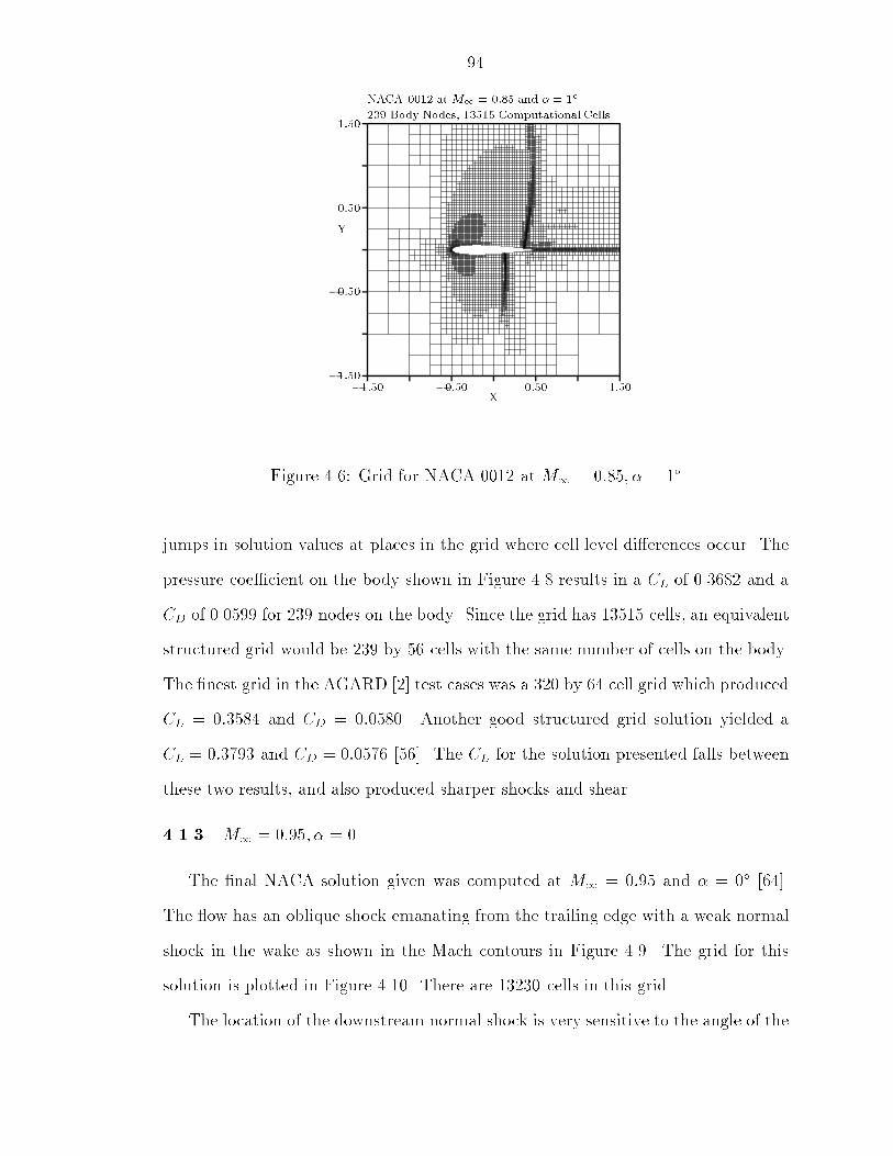
94�1:50 �0:50 0:50 1:50�1:50�0:500:501:50

XY 239 Body Nodes, 13515 Computational Cells.NACA 0012 at M1 = 0:85 and � = 1�Figure 4.6: Grid for NACA 0012 at M1 = 0:85; � = 1�jumps in solution values at places in the grid where cell level di�erences occur. Thepressure coe�cient on the body shown in Figure 4.8 results in a CL of 0.3682 and aCD of 0.0599 for 239 nodes on the body. Since the grid has 13515 cells, an equivalentstructured grid would be 239 by 56 cells with the same number of cells on the body.The �nest grid in the AGARD [2] test cases was a 320 by 64 cell grid which producedCL = 0:3584 and CD = 0:0580. Another good structured grid solution yielded aCL = 0:3793 and CD = 0:0576 [56]. The CL for the solution presented falls betweenthese two results, and also produced sharper shocks and shear.4.1.3 M1 = 0:95; � = 0The �nal NACA solution given was computed at M1 = 0:95 and � = 0� [64].The ow has an oblique shock emanating from the trailing edge with a weak normalshock in the wake as shown in the Mach contours in Figure 4.9. The grid for thissolution is plotted in Figure 4.10. There are 13230 cells in this grid.The location of the downstream normal shock is very sensitive to the angle of the

95�1:50 �0:50 0:50 1:50�1:50�0:500:501:50

XY Mach ContoursNACA 0012 at M1 = 0:85 and � = 1�0.8000.8400.8800.8400.8800.800 Fmin 0.029Fst 0.040Finc 0.040Fmax 1.440

Figure 4.7: Mach Contours for NACA 0012 at M1 = 0:85; � = 1�1:200:40�0:40�1:20Cp Pressure Coe�cient on the Body.NACA 0012 at M1 = 0:85 and � = 1�

Figure 4.8: Pressure Coe�cient on Body of NACA 0012 at M1 = 0:85; � = 1�

96�3:0 1:0 5:0 9:0�6:0�2:02:06:0 XY Mach ContoursNACA 0012 At M1 = 0:95; � = 0�0.9000.9501.000 Fmin 0.012Fst 0.050Finc 0.050Fmax 1.462

Figure 4.9: Mach Contours for NACA 0012 at M1 = 0:95; � = 0��3:0 1:0 5:0 9:0�6:0�2:02:06:0 XY 264 Body Nodes, 13230 Computational Cells.NACA 0012 At M1 = 0:95; � = 0�

Figure 4.10: Grid for NACA 0012 at M1 = 0:95; � = 0�

970:00 0:50 1:00 1:50�0:500:000:501:00

XY Mach ContoursNACA 0012 At M1 = 0:95; � = 0�1.3501.3001.250 Fmin 0.012Fst 0.050Finc 0.050Fmax 1.462Figure 4.11: Detail Mach Contours for NACA 0012 at M1 = 0:95; � = 0�oblique shock. In turn, the angle of the oblique shock is very sensitive to the Machnumber on the body just upstream of the trailing edge. Figures 4.11 and 4.12 showa blowup of the Mach contours and grid in the trailing edge region of the ow.To guarantee an accurate value of Mach number on the body before the obliqueshock, the expansion region must have su�cient grid resolution. The cell length-scale weighting described in Section 2.4 ensures that this is the case by re�ning notjust the shocks, but also this expansion region. The position of the normal shockimproves with each solution re�nement applied, since both the normal shock and theexpansion area on the airfoil are re�ned. A plot of the normal shock location is givenin Figure 4.13 as a Mach number cut at y = 0 for each of �ve di�erent solution levels.The shock location converges to a location 3.41 chords behind the trailing edge ofthe airfoil. A \best" solution was obtained on a 2049 by 765 O-type structured gridwhich resulted in a shock location 3.35 chords downstream of the trailing edge [64].

980:00 0:50 1:00 1:50�0:500:000:501:00

XY 264 Body Nodes, 13230 Computational Cells.NACA 0012 At M1 = 0:95; � = 0�Figure 4.12: Detail Grid for NACA 0012 at M1 = 0:95; � = 0�

1:50 2:50 3:50 4:500:700:901:101:30Distance From Trailing EdgeM Mach Number Cuts At Y=0 For Various Re�nement LevelsNACA 0012 At M1 = 0:95; � = 0�1 2 3 4 5

Figure 4.13: Normal Shock Location for NACA 0012 at M1 = 0:95; � = 0�

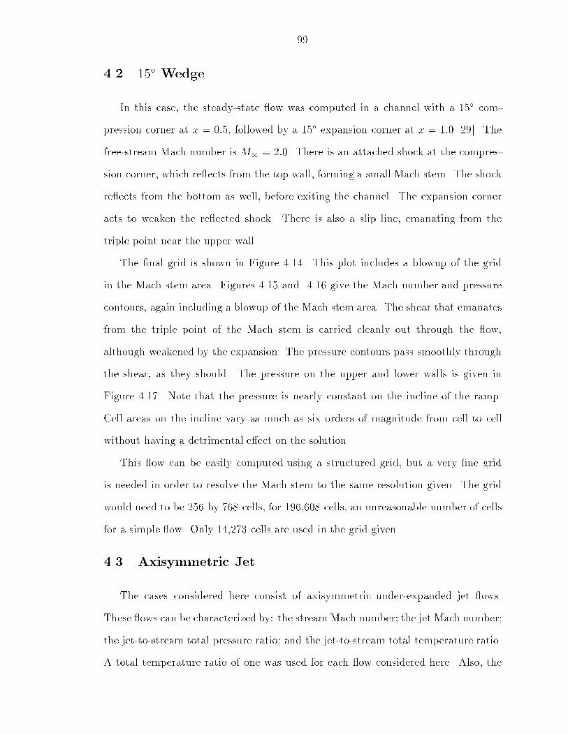
994.2 15� WedgeIn this case, the steady-state ow was computed in a channel with a 15� com-pression corner at x = 0:5, followed by a 15� expansion corner at x = 1:0 [29]. Thefree-stream Mach number is M1 = 2:0. There is an attached shock at the compres-sion corner, which re ects from the top wall, forming a small Mach stem. The shockre ects from the bottom as well, before exiting the channel. The expansion corneracts to weaken the re ected shock. There is also a slip line, emanating from thetriple point near the upper wall.The �nal grid is shown in Figure 4.14. This plot includes a blowup of the gridin the Mach stem area. Figures 4.15 and 4.16 give the Mach number and pressurecontours, again including a blowup of the Mach stem area. The shear that emanatesfrom the triple point of the Mach stem is carried cleanly out through the ow,although weakened by the expansion. The pressure contours pass smoothly throughthe shear, as they should. The pressure on the upper and lower walls is given inFigure 4.17. Note that the pressure is nearly constant on the incline of the ramp.Cell areas on the incline vary as much as six orders of magnitude from cell to cellwithout having a detrimental e�ect on the solution.This ow can be easily computed using a structured grid, but a very �ne gridis needed in order to resolve the Mach stem to the same resolution given. The gridwould need to be 256 by 768 cells, for 196,608 cells, an unreasonable number of cellsfor a simple ow. Only 14,273 cells are used in the grid given.4.3 Axisymmetric JetThe cases considered here consist of axisymmetric under-expanded jet ows.These ows can be characterized by: the streamMach number; the jet Mach number;the jet-to-stream total pressure ratio; and the jet-to-stream total temperature ratio.A total temperature ratio of one was used for each ow considered here. Also, the

1000:00 1:00 2:00 3:000:001:00 XY 14273 Computational Cells.

Figure 4.14: Grid for 15� Wedge at M1 = 2:0

1010:00 1:00 2:00 3:000:001:00 XY Fmin 0.575Fst 0.580Finc 0.040Fmax 2.0021.4452.000 1.9562.0001.4601.500 1.1401.180

Figure 4.15: Mach Contours for 15� Wedge at M1 = 2:0

1020:00 1:00 2:00 3:000:001:00 XY Fmin 0.65Fst 0.70Finc 0.10Fmax 3.320.7231.5680.714 0.714 1.5001.400 2.3002.200Figure 4.16: Pressure Contours for 15� Wedge at M1 = 2:0

0:00 1:00 2:00 3:000:501:502:503:50XP Lower Wall Lower WallUpper Wall

Free-streamFigure 4.17: Wall Pressure for 15� Wedge at M1 = 2:0

103CL

Expansion Mach Disk

Reflected ShockExternal Shock

Jet Boundary

Intercepting ShockSlip Line

ExpansionFigure 4.18: Schematic of an Under-Expanded Jet with Mach Diskjet Mach number was set equal to the stream Mach number for each case. A singleMach number will be considered here. The primary e�ect of Mach number, when thejet and stream Mach number are equal, is the strength and scale of the ow. Thusa ow with larger Mach number would have stronger features which would occurfarther downstream of the end of the nozzle. A schematic of an under-expanded jetwith a Mach disk is pictured in Figure 4.18. These cases highlight the solution-basedadaptation of the code, since a wide range of feature strengths are evident in these ows.4.3.1 M = 1:25; P0j=P0s = 20An under-expanded axisymmetric jet at Mach 1.25 and jet-to-stream total pres-sure ratio of 20 is considered �rst. The grid and Mach contours are given in Fig-ures 4.19 and 4.20. The re�nement criterion has detected the external shock, theintercepting shock and its re ection, the jet boundary, and the rapid expansion atthe nozzle exit. Few of these ow features are visible for plots of density or pres-sure, since the expansion at the nozzle exit dominates. The contours of density andpressure are shown in Figures 4.21 and 4.22.

104�6:0 6:0 18:0 30:00:0

18:0XY 27045 Computational Cells.Axisymmetric Jet At M = 1:25; P0j =P0s = 20

Figure 4.19: Grid for Jet at M = 1:25; P0j=P0s = 20�6:0 6:0 18:0 30:00:0

18:0XY Mach ContoursAxisymmetric Jet At M = 1:25; P0j =P0s = 20 Fmin 0.33Fst 0.40Finc 0.20Fmax 7.521.25 1.201.25 1.00

Figure 4.20: Mach Contours for Jet at M = 1:25; P0j=P0s = 20

105�6:0 6:0 18:0 30:00:0

18:0XY Density ContoursAxisymmetric Jet At M = 1:25; P0j =P0s = 20 Fmin 0.07Fst 0.50Finc 0.50Fmax 20.0020.001.00 0.50 1.00 1.00

Figure 4.21: Density Contours for Jet at M = 1:25; P0j=P0s = 20�6:0 6:0 18:0 30:00:0

18:0XY Pressure ContoursAxisymmetric Jet At M = 1:25; P0j =P0s = 20 Fmin 0.01Fst 0.40Finc 0.40Fmax 14.29

14.2860.714 0.800 0.800 0.800Figure 4.22: Pressure Contours for Jet at M = 1:25; P0j=P0s = 20

106�3:0 3:0 9:0 15:00:0

9:0XY 22251 Computational Cells.Axisymmetric Jet At M = 1:25; P0j =P0s = 5

Figure 4.23: Grid for Jet at M = 1:25; P0j=P0s = 54.3.2 M = 1:25; P0j=P0s = 5This case shows the e�ect of decreasing the jet-to-stream total pressure ratio to5 from 20. The ow is similar to the previous case, although many of the featuresare considerably weaker and closer to the nozzle exit. The grid and Mach contoursfor this case are given in Figures 4.23 and 4.24. Again the ow features are wellresolved, despite the disparate strengths of the features.4.3.3 M = 1:25; P0j=P0s = 50When the jet-to-stream total pressure ratio is increased to 50, the interceptingshock no longer simply re ects o� the axis of symmetry; instead, a large Mach diskis formed. The slip line emanating from the Mach triple point is as apparent as thejet boundary. Also, the jet boundary is more highly curved due to the lower pressureof the stream. The grid for this case is pictured in Figure 4.25. Figure 4.26 showsthe Mach contours.

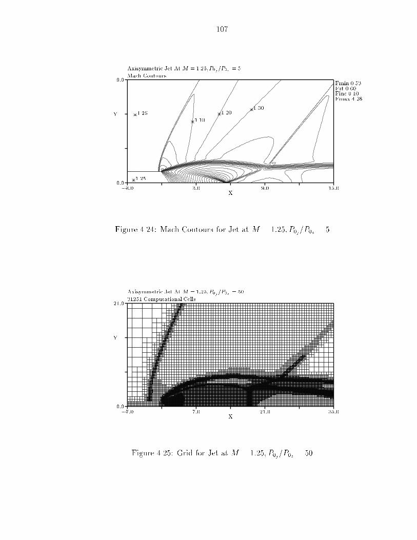
107�3:0 3:0 9:0 15:00:0

9:0XY Mach ContoursAxisymmetric Jet At M = 1:25; P0j =P0s = 5

1.251.25 1.10 1.20 1.30 Fmin 0.53Fst 0.60Finc 0.10Fmax 4.28Figure 4.24: Mach Contours for Jet at M = 1:25; P0j=P0s = 5�7:0 7:0 21:0 35:00:0

21:0XY 31251 Computational Cells.Axisymmetric Jet At M = 1:25; P0j =P0s = 50

Figure 4.25: Grid for Jet at M = 1:25; P0j=P0s = 50

108�7:0 7:0 21:0 35:00:0

21:0XY Mach ContoursAxisymmetric Jet At M = 1:25; P0j =P0s = 50

1.251.25 1.00 1.20 0.27Fmin 0.13Fst 0.20Finc 0.20Fmax 9.63

Figure 4.26: Mach Contours for Jet at M = 1:25; P0j=P0s = 504.3.4 M = 1:25; P0j=P0s = 100When the jet-to-stream total pressure ratio is increased further to 100, the Machdisk becomes larger, and moves farther downstream of the nozzle lip. The ow is,in all other respects, similar to the previous Mach disk case. Figures 4.27 and 4.28plot the grid and Mach contours, respectively.4.4 Multi-Element AirfoilsThree di�erent multi-element airfoils will be examined, each at purely subsonicspeeds. These three cases have a higher degree of geometric complexity than thecases already considered, but the grid generation for these con�gurations is no morecomplicated than for the simplest of geometries. The initial grids generated showproper resolution of high curvature portions of the bodies, and amply resolve the ow features.

109�7:0 7:0 21:0 35:00:0

21:0XY 28275 Computational Cells.Axisymmetric Jet At M = 1:25; P0j =P0s = 100

Figure 4.27: Grid for Jet at M = 1:25; P0j=P0s = 100�7:0 7:0 21:0 35:00:0

21:0XY Mach ContoursAxisymmetric Jet At M = 1:25; P0j =P0s = 100

1.251.25 0.80 1.00 1.20 0.26Fmin 0.17Fst 0.20Finc 0.20Fmax 9.98

Figure 4.28: Mach Contours for Jet at M = 1:25; P0j=P0s = 100

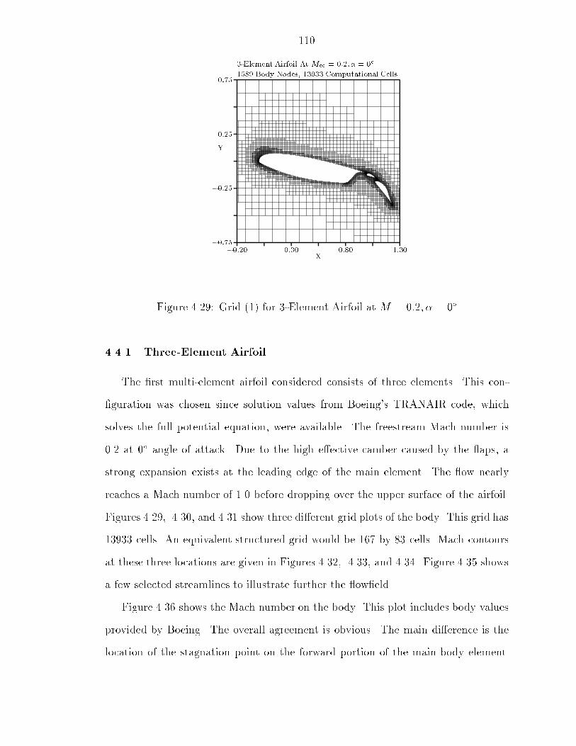
110�0:20 0:30 0:80 1:30�0:75�0:250:250:75

XY 1589 Body Nodes, 13933 Computational Cells.3-Element Airfoil At M1 = 0:2; � = 0�Figure 4.29: Grid (1) for 3-Element Airfoil at M = 0:2; � = 0�4.4.1 Three-Element AirfoilThe �rst multi-element airfoil considered consists of three elements. This con-�guration was chosen since solution values from Boeing's TRANAIR code, whichsolves the full potential equation, were available. The freestream Mach number is0.2 at 0� angle of attack. Due to the high e�ective camber caused by the aps, astrong expansion exists at the leading edge of the main element. The ow nearlyreaches a Mach number of 1.0 before dropping over the upper surface of the airfoil.Figures 4.29, 4.30, and 4.31 show three di�erent grid plots of the body. This grid has13933 cells. An equivalent structured grid would be 167 by 83 cells. Mach contoursat these three locations are given in Figures 4.32, 4.33, and 4.34. Figure 4.35 showsa few selected streamlines to illustrate further the ow�eld.Figure 4.36 shows the Mach number on the body. This plot includes body valuesprovided by Boeing. The overall agreement is obvious. The main di�erence is thelocation of the stagnation point on the forward portion of the main body element.

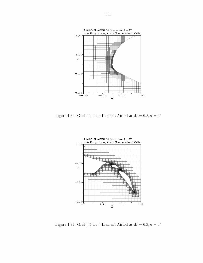
111�0:060 �0:020 0:020 0:060�0:060�0:0200:0200:060

XY 1589 Body Nodes, 13933 Computational Cells.3-Element Airfoil At M1 = 0:2; � = 0�Figure 4.30: Grid (2) for 3-Element Airfoil at M = 0:2; � = 0�

0:70 0:90 1:10 1:30�0:50�0:30�0:100:10XY 1589 Body Nodes, 13933 Computational Cells.3-Element Airfoil At M1 = 0:2; � = 0�

Figure 4.31: Grid (3) for 3-Element Airfoil at M = 0:2; � = 0�

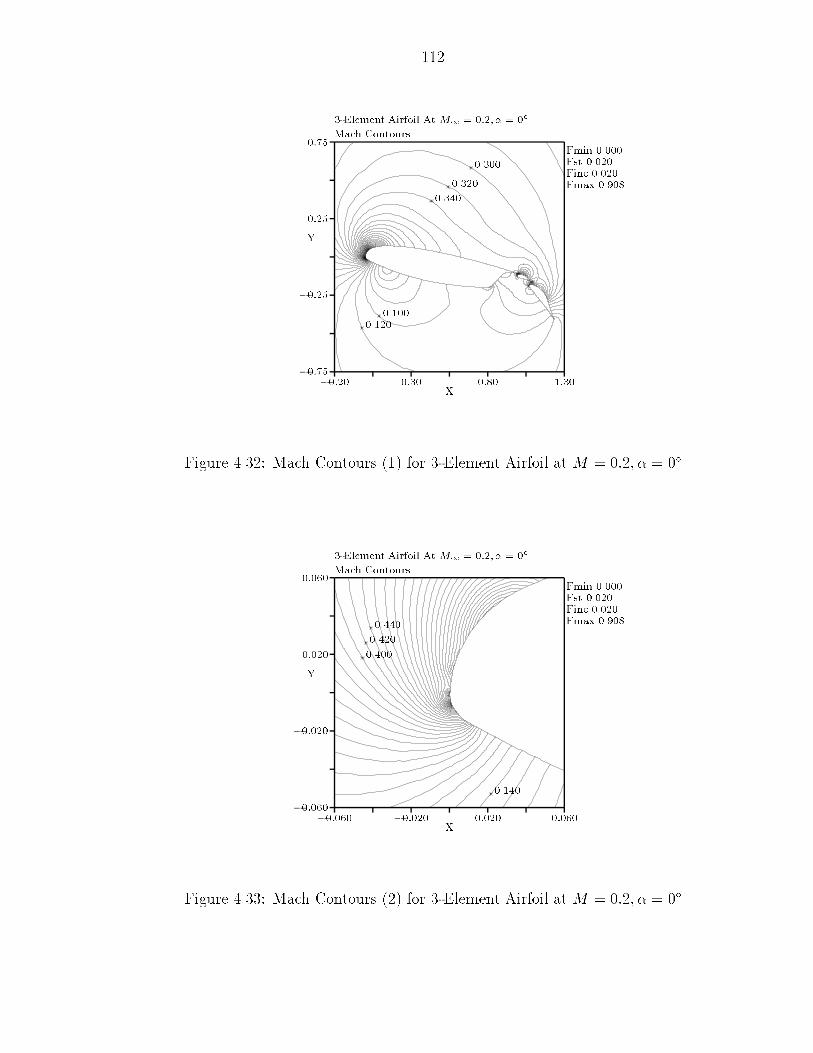
112�0:20 0:30 0:80 1:30�0:75�0:250:250:75

XY Mach Contours3-Element Airfoil At M1 = 0:2; � = 0�0.3400.3200.3000.1200.100Fmin 0.000Fst 0.020Finc 0.020Fmax 0.908

Figure 4.32: Mach Contours (1) for 3-Element Airfoil at M = 0:2; � = 0��0:060 �0:020 0:020 0:060�0:060�0:0200:0200:060

XY Mach Contours3-Element Airfoil At M1 = 0:2; � = 0�0.4000.4200.4400.140

Fmin 0.000Fst 0.020Finc 0.020Fmax 0.908Figure 4.33: Mach Contours (2) for 3-Element Airfoil at M = 0:2; � = 0�

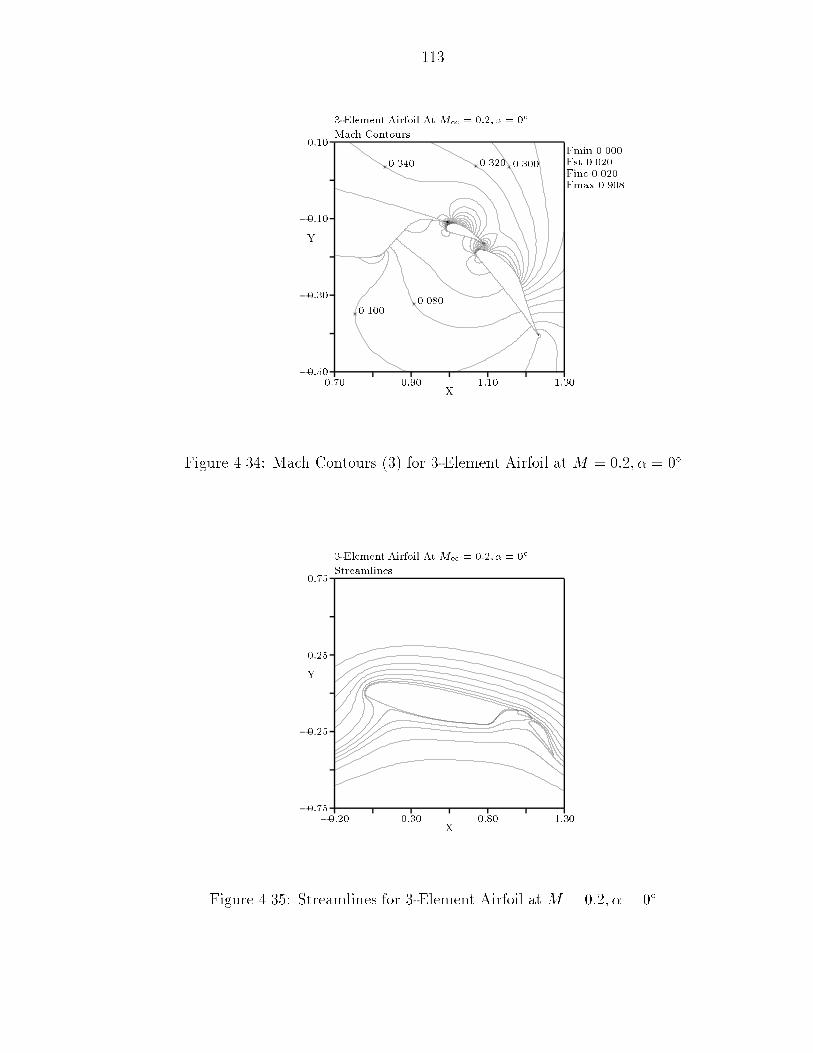
1130:70 0:90 1:10 1:30�0:50�0:30�0:100:10

XY Mach Contours3-Element Airfoil At M1 = 0:2; � = 0�0.340 0.3200.100 0.080 0.300 Fmin 0.000Fst 0.020Finc 0.020Fmax 0.908Figure 4.34: Mach Contours (3) for 3-Element Airfoil at M = 0:2; � = 0�

�0:20 0:30 0:80 1:30�0:75�0:250:250:75XY Streamlines3-Element Airfoil At M1 = 0:2; � = 0�

Figure 4.35: Streamlines for 3-Element Airfoil at M = 0:2; � = 0�

1140:000:400:801:20M Mach Number On The Body3-Element Airfoil At M1 = 0:2; � = 0� ComputedBoeing

Figure 4.36: Mach Number on Body for 3-Element Airfoil at M = 0:2; � = 0�The stagnation point produced by this code was slightly farther ahead, resulting in asmaller leading edge expansion and a larger Mach number on the lower surface of themain element. The e�ect of this di�erence can also be seen on the pressure coe�cienton the body as shown in Figure 4.37. This code produced a slightly smaller pressurecoe�cient peak at the leading edge. The two aps, however, agree extremely wellwith the Boeing results. The computed CL for this con�guration is 5.162; the CDcomputed is 0.178.Again, despite large variations in the cell size on the body (the area of the smallestcut cell is 106 smaller than that of its uncut neighbor) the solution is smooth. Thetotal pressure loss, 1�p0=p01 , is shown in Figure 4.38. The loss is near 0.2%, exceptfor a spike at the trailing edge of each body.4.4.2 Two-Element AirfoilThis case consists of a two-elementKarman-Tre�tz airfoil and ap atM1 = 0:125and � = 0� [33]. An exact incompressible potential solution exists for this case that

1154:0�4:0�12:0�20:0Cp Pressure Coe�cient On The Body3-Element Airfoil At M1 = 0:2; � = 0� ComputedBoeing

Figure 4.37: Pressure Coe�cient on Body for 3-Element Airfoil at M = 0:2; � = 0��0:00500:00500:01500:02501� p0=p01 1� p0=p01 On The Body3-Element Airfoil At M1 = 0:2; � = 0�

Figure 4.38: 1� p0=p01 on Body for 3-Element Airfoil at M = 0:2; � = 0�

116�0:30 0:30 0:90 1:50�0:90�0:300:300:90

XY 1187 Body Nodes, 10827 Computational Cells.2-Element Airfoil At M1 = 0:125;� = 0�Figure 4.39: Grid for 2-Element Airfoil at M = 0:125; � = 0�may be used for comparison. At this Mach number, the compressibility e�ects arevery small. The grid for this ow in pictured in Figure 4.39. This grid has 10827cells. An equivalent structured grid would be 147 by 73 cells. The Mach contoursare given in Figure 4.40. The exact surface pressure coe�cient is plotted on top ofthe computed values in Figure 4.41. The solutions show good agreement, with theexception of a stagnation point on the main element slightly forward, resulting in aslightly smaller expansion on the leading edge. The agreement on the rear element isexcellent. The computed CL for this con�guration is 1.936, while CD is 0.0237. Thetotal pressure loss is shown in Figure 4.42. The loss is near zero, except for a spikesat the leading and trailing edges of each body. Signi�cant additional re�nement ofthe leading-edge region does not improve the solution.4.4.3 Four-Element AirfoilThis case is similar to the previous case in that an exact incompressible solution isknown. The freestream Mach number is 0.125 for this four-element airfoil. The grid

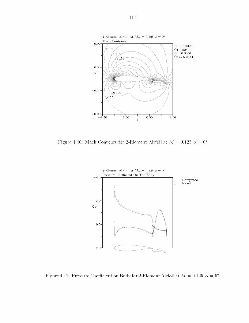
117�0:30 0:30 0:90 1:50�0:90�0:300:300:90

XY Mach Contours2-Element Airfoil At M1 = 0:125;� = 0�0.1400.1450.1500.1100.105Fmin 0.0028Fst 0.0050Finc 0.0050Fmax 0.2454

Figure 4.40: Mach Contours for 2-Element Airfoil at M = 0:125; � = 0�2:00:0�2:0�4:0Cp Pressure Coe�cient On The Body2-Element Airfoil At M1 = 0:125;� = 0� ComputedExact

Figure 4.41: Pressure Coe�cient on Body for 2-Element Airfoil atM = 0:125; � = 0�

118�0:00100:00100:00300:00501� p0=p01 1� p0=p01 On The Body2-Element Airfoil At M1 = 0:125;� = 0�

Figure 4.42: 1 � p0=p01 on Body for 2-Element Airfoil at M = 0:125; � = 0�for this airfoil is given in Figure 4.43. More detailed portions of the grid are shown inFigures 4.44 and 4.45 This grid has 14204 cells. An equivalent structured grid wouldbe 168 by 84 cells. The Mach contours corresponding to these grid plots are given inFigures 4.46, 4.47, and 4.48. The known exact solution for the pressure coe�cient onthe body is again plotted on top of the computed values shown in Figure 4.49. Again,the solutions show good agreement except for the slight di�erence in the leading edgeexpansions. The lower surfaces and the trailing edge aps show excellent agreement,however. Finally, the total pressure loss is shown in Figure 4.50. The loss is around0.1%, except for the leading and trailing edge spikes on each body.

119�4:0 �1:0 2:0 5:0�5:0�2:01:04:0 XY 1620 Body Nodes, 14204 Computational Cells.4-Element Airfoil At M1 = 0:125;� = 0�

Figure 4.43: Grid (1) for 4-Element Airfoil at M = 0:01; � = 0��2:50 �2:00 �1:50 �1:00�0:75�0:250:250:75

XY 1620 Body Nodes, 14204 Computational Cells.4-Element Airfoil At M1 = 0:125;� = 0�Figure 4.44: Grid (2) for 4-Element Airfoil at M = 0:01; � = 0�

1201:0 2:0 3:0 4:0�2:0�1:00:01:0 XY 1620 Body Nodes, 14204 Computational Cells.4-Element Airfoil At M1 = 0:125;� = 0�

Figure 4.45: Grid (3) for 4-Element Airfoil at M = 0:01; � = 0��4:0 �1:0 2:0 5:0�5:0�2:01:04:0 XY Mach Contours4-Element Airfoil At M1 = 0:125;� = 0�0.1800.1700.1600.1000.090

Fmin 0.001Fst 0.010Finc 0.010Fmax 0.291Figure 4.46: Mach Contours (1) for 4-Element Airfoil at M = 0:01; � = 0�

121�2:50 �2:00 �1:50 �1:00�0:75�0:250:250:75

XY Mach Contours4-Element Airfoil At M1 = 0:125;� = 0�0.1700.180 0.190 0.2000.080 0.070

Fmin 0.001Fst 0.010Finc 0.010Fmax 0.291Figure 4.47: Mach Contours (2) for 4-Element Airfoil at M = 0:01; � = 0�

1:0 2:0 3:0 4:0�2:0�1:00:01:0 XY Mach Contours4-Element Airfoil At M1 = 0:125;� = 0�0.180 0.170 0.1600.1800.070 Fmin 0.001Fst 0.010Finc 0.010Fmax 0.291Figure 4.48: Mach Contours (3) for 4-Element Airfoil at M = 0:01; � = 0�

1221:2�1:2�3:6�6:0Cp Pressure Coe�cient On The Body4-Element Airfoil At M1 = 0:125;� = 0� ComputedExact

Figure 4.49: Pressure Coe�cient on Body for 4-Element Airfoil at M = 0:01; � = 0��0:00100:00100:00300:00501� p0=p01 1� p0=p01 On The Body4-Element Airfoil At M1 = 0:125;� = 0�

Figure 4.50: 1 � p0=p01 on Body for 4-Element Airfoil at M = 0:125; � = 0�

CHAPTER VCONCLUSIONSThis thesis is brought to a close with a summary of the contributions of this workas well as some suggestions for ways in which the work could be usefully extended.5.1 SummaryA method has been developed by which the solution of the steady-state 2-D Eulerequations can be obtained using solution-based re�nement for ows around bodieswith arbitrary geometric complexity.A quadtree cell-based data structure is used to control the unstructured grid.The data tree is made up of a list of cells with pointers to a cell's parent and fourchildren (if they exist). Connectivity information is obtained from the data tree viathis parent/child relationship.The initial grid is generated with a minimum of user input for any complexcon�guration. The user need only specify a set of points de�ning the bodies, thebase grid resolution, and cell size thresholds for the initial grid, cut-cell re�nement,and curvature re�nement. With proper thresholds, the grid is automatically adaptedto the curvature of a body, providing the resolution required to resolve that bodyadequately.The grid is also improved through the use of solution-based re�nement. Once asolution has converged to a steady state, solution-based gradient information (specif-123

124ically a blend of jr � uj and jr � uj) is used to ag cells for dividing or coarsening.This process ensures that the grid resolution matches the length scales of the local ow �eld.Small cut cells are created by the arbitrary way that the Cartesian grid cutsthrough the body. This problem is easily overcome, however, by using local time-stepping, coupled with a linear reconstruction method. This allows the solution toconverge as accurately as if the small cells did not exist. The reconstruction methodwas designed speci�cally for unstructured grids, and provides an accurate gradientof cell values as long as at least three non-collinear neighbor cells are available.The solution is advanced in time with a multi-stage time stepping scheme. Multi-grid convergence acceleration was also employed. The tree-based method is ideal formultigrid since coarser grid levels already exist, as well as all of the needed grid-levelcommunication.Test cases include internal, external, and axisymmetric ows. For the NACA andmulti-element airfoils, the outer boundary could be placed at great distances fromthe airfoil without signi�cantly increasing the total number of cells, thus eliminatingthe need for sophisticated outer boundary conditions. The wedge case showed thatvery �ne features can be resolved without a large number of cells throughout thedomain as in structured grids methods.5.2 ConclusionsOne pressing need for CFD is the ability to generate, automatically and robustly,a grid for complex three-dimensional con�gurations, and to compute stable and ac-curate ow solutions about that con�guration. Many approaches are being used atthe present, but no one method has emerged as the best option for grid generationand ow solution about arbitrarily complex geometries.A Cartesian grid approach shows great promise as a method to overcome these

125problems. But, Cartesian grids do have their share of di�culties to overcome. Anyarbitrarily complex geometry can be cut out of a Cartesian grid, but the resultinggrid is a very poor representation of the body. A uniform Cartesian grid �ne enoughto resolve a body adequately would require many more cells than were needed awayfrom the body, thereby requiring unreasonable resources to obtain a solution. Thesolution to this problem is adaptation. A Cartesian grid which can be automaticallyand robustly adapted to a body to ensure that each of its features is adequatelyresolved is needed. Indeed, methods are being developed which are coming close tothis ideal for fully arbitrary three-dimensional con�gurations. Especially promisingis the reduction in total number of cells needed to create these grids. Cells can beadded only where resolution of the body requires them. This is not only importantin terms of physical memory usage to store the information, but also in terms of thereal time required to generate the grid and compute ow solutions.Automatic Cartesian grid generation is not the whole picture, however. The ow solution is also required. Here again, Cartesian grids have some problems.The somewhat arbitrary way that bodies are cut out of a Cartesian grid can createa huge disparity in the sizes of neighboring cells. This issue has been addressedto some degree in two dimensions in this thesis, but questions remain about howwell these methods will carry over to three dimensions. Flow solution methods forunstructured grids is currently a widely researched topic, and new innovations mayhave a large e�ect on the e�ectiveness of ow solution on Cartesian grids. Anotherimportant issue to be resolved is how solution to the full Navier-Stokes equations, orany other set of conservation equations, can �t into the Cartesian framework. Willnew methods need to be developed, or can existing methods be modi�ed to provide ow solutions? One huge bene�t to ow solution using a Cartesian grid is that gridadaptation has already been developed in creating the grid. Using additional gridadaptation by solution-based information will provide more accurate solutions for

126less cost.The results of the method presented in this thesis show that this Cartesian gridapproach is viable. Second-order global accuracy is obtained for the given computedsolutions. These solutions compare very favorably not only with the GAMM andAGARD benchmark solutions, but also with exact incompressible solutions. Thenumber of cells required to obtain these solutions is greatly reduced due to adapta-tion. In fact, comparable structured grid solutions require from two to ten times thenumber of cells needed for the Cartesian method. However, compared to a structuredgrid approach, memory overhead is around 25%, and run-time overhead is around30%. The run-time scales linearly with the number of cells, due to multigrid. Over-all, the ow solutions computed with this Cartesian approach with 15 the number ofcells would take around 13 of the time to compute, with the same solution accuracy.Which technologies will still be in use ten years from now cannot be answered. ButCartesian grid methods with adaptation show great promise to be at the forefront.Cartesian grids will one day be used in CFD for automatic, robust, and e�cient gridgeneration and ow solution for complex three-dimensional con�gurations.5.3 Future WorkThere are a number of areas of research where this work could be naturallyextended. The �rst extension is unsteady ow. The most obvious approach is tomerge cut cells. Any cell which is cut by the body would be merged with one ofits uncut neighbor cells. This results in a slight accuracy loss on the body, but thetime-step from the neighbor cell is used rather than the small time-step from thecut cell. This does not address the disparate time-steps from cells on di�erent gridlevels, where more sophisticated time-step schemes are needed [10].Another likely extension of this work is to compute ow solutions of the Navier-Stokes equations. The main di�culty here is the viscous layer should have cells with

127a large aspect ratio and are aligned with the body. Allowing these \non-Cartesian"cuts requires a much more sophisticated data-structure. In this case, a binary treemay be more useful. Discretization of the viscous terms is also not a trivial task, andthe smoothness of the grid becomes much more important [12]. In fact, the work inthis thesis could be extended to any set of conservation equations, including owswith chemical reactions or magnetic �elds.The most obvious extension to this work comes in extending the algorithm tothree dimensions. The appropriate data structure in the three-dimensional case isan octree, with each parent cell being divided into eight children cells. The bodyde�nition is one obvious di�culty to overcome. De�ning a body surface from a setof points and incorporating that information into a code is a di�cult task. Memoryusage and computer speed become much more important as well.

BIBLIOGRAPHY

128

129BIBLIOGRAPHY[1] M. J. Aftosmis and N. Kroll, \A quadrilateral based second-order TVD methodfor unstructured adaptive meshes," AIAA Paper 91-0124, 1991.[2] AGARD Subcommittee C, \Test cases for inviscid ow �eld methods." AGARDAdvisory Report 211, 1986.[3] T. J. Barth, \On unstructured grids and solvers," in Computational Fluid Dy-namics, Von K�arm�an Institute for Fluid Dynamics, Lecture Series 1990-04, 1990.[4] T. J. Barth and P. O. Frederickson, \Higher order solution of the Euler equationson unstructured grids using quadratic reconstruction," AIAA Paper 90-0013,1990.[5] S. A. Bayyuk, K. G. Powell, and B. van Leer, \A simulation technique for 2-D unsteady inviscid ows around arbritrarily moving and deforming bodies ofarbitrary geometry," AIAA Paper 93-3391, 1993.[6] M. J. Berger and P. Colella, \Local adaptive mesh re�nement for shock hydro-dynamics," Tech. Rep. UCRL-97196, Lawrence Livermore National Laboratory,1987.[7] M. J. Berger and A. Jameson, \Automatic adaptive grid re�nement for the Eulerequations," AIAA Journal, vol. 23, 1985.[8] M. J. Berger and R. J. LeVeque, \A rotated di�erence scheme for Cartesiangrids in complex geometries," AIAA Paper 91-1602, 1991.[9] W. L. Briggs, \A multigrid tutorial," 1987.[10] Y.-L. Chiang, Simulation of Unsteady Inviscid Flow on an Adaptively Re�nedCartesian Grid. PhD thesis, University of Michigan, 1991.[11] D. K. Clarke, M. D. Salas, and H. A. Hassan, \Euler calculations for muti-element airfoils using Cartesian grids," AIAA Journal, vol. 24, 1986.[12] W. J. Coirier, \Cartesian-cell based grid generation and adaptive mesh re�ne-ment," in NASA Workshop on Unstructured Grid Generation, NASA CP 10119,1993.

130[13] W. J. Coirier and K. G. Powell, \An accuracy assessment of cartesian-meshapproaches for the Euler equations," AIAA Paper 93-3335, 1993.[14] S. D. Connell and D. G. Holmes, \A 3d unstructured adaptive multigrid schemefor the Euler equations," AIAA Paper 93-3339, 1993.[15] J. F. Dannenho�er III, \A comparison of adaptive-grid redistribution and em-bedding for steady transonic ows," International Journal for Numerical Meth-ods in Engineering, vol. 32, pp. 653{663, 1991.[16] J. F. Dannenho�er III, \Computer-aided block structuring through the use ofoptimization and expert system techniques," in AIAA 10th Computational FluidDynamics Conference, 1991.[17] D. De Zeeuw and K. G. Powell, \An adaptively-re�ned carterian mesh solverfor the Euler equations," Journal of Computational Physics, vol. 104, no. 1,pp. 56{68, 1993.[18] P. R. Eiseman, \Coordinate generation with precise controls over mesh proper-ties," Journal of Computational Physics, vol. 47, 1982.[19] P. R. Eiseman, \Adaptive grid generation," Computer Methods in Applied Me-chanics and Engineering, vol. 64, 1987.[20] B. Epstein, A. L. Luntz, and A. Nachshon, \Multigrid Euler solver about ar-bitrary aircraft con�gurations with Cartesian grids and local re�nement," inAIAA 9th Computational Fluid Dynamics Conference, 1989.[21] S. K. Godunov, \A �nite-di�erence method for the numerical computation anddiscontinuous solutions of the equations of uid dynamics," MatematicheskiiSbornik, vol. 47, pp. 271{306, 1959.[22] P. W. Hemker, H. T. M. van der Maarel, and C. T. H. Everaars, \BASIS: adata structure for adaptive multigrid computations," Center for Mathematicsand Computer Science Report NM-R9014, Amsterdam, 1990.[23] D. G. Holmes and D. D. Snyder, \The generation of unstructured triangularmeshes using Delaunay triangulation," in Proceedings of the Second Confer-ence on Grid Generation in Computational Fluid Dynamics, Pineridge Press,Swansea, 1988.[24] J. G. Kallinderis and J. R. Baron, \Adaptation methods for a new Navier-Stokesalgorithm," in AIAA 8th Computational Fluid Dynamics Conference, 1987.[25] S. R. Kennon, \A vectorized Delaunay triangulation scheme for non-convexdomains with automatic nodal point generation," AIAA Paper 88-0314, 1988.

131[26] S. R. Kennon and D. A. Anderson, \Unstructured grid adaption for non-convexdomains," in Numerical Grid Generation In Computational Fluid Mechanics '88(S. Sengupta, J. Ha�user, P. R. Eiseman, and J. F. Thompson, eds.), PineridgePress, 1988.[27] H. J. Kim and J. F. Thompson, \Three dimensional adaptive grid generationon a composite block grid," AIAA Paper 88-0311, 1988.[28] K. Kusunose, L. Wigton, and P. Meredith, \A rapidly converging vis-cous/inviscid coupling code for multi-element airfoil con�gurations," AIAA Pa-per 91-0177, 1991.[29] D. Levy, Use of a Rotated Riemann Solver for the Two-Dimensional Euler Equa-tions. PhD thesis, The University of Michigan, 1990.[30] M. S. Liou, B. van Leer, and J. S. Shuen, \Splitting of inviscid uxes for realgases," Journal of Computational Physics, vol. 87, 1990.[31] R. L�ohner, \Some useful data structures for the generation of unstructuredgrids," Communications in Applied and Numerical Mathematics, vol. 4, pp. 123{135, 1988.[32] R. L�ohner and P. Parikh, \Generation of three-dimensional unstructured gridsby the advancing-front method," AIAA Paper 88-0515, 1988.[33] D. J. Mavriplis, \Accurate multigrid solution of the Euler equations on unstruc-tured and adaptive meshes," AIAA Journal, vol. 28, 1990.[34] D. J. Mavriplis, \Adaptive mesh generation for viscous ows using Delaunaytriangulation," Journal of Computational Physics, vol. 90, 1990.[35] J. E. Melton, F. Y. Enomoto, and M. J. Berger, \3D automatic Cartesian gridgeneration for Euler equations," AIAA Paper 93-3386, 1993.[36] J. E. Melton, S. D. Thomas, and G. Cappuccio, \Unstructured Euler ow solu-tions using hexahedral cell re�nement," AIAA Paper 91-0637, 1991.[37] J.-D. M�uller, \Proven angular bounds and stretched triangulations with thefrontal delaunay method," AIAA Paper 93-3347, 1993.[38] K. Nakahashi, \An automatic grid generator for the unstructured upwindmethod," in AIAA 9th Computational Fluid Dynamics Conference, 1989.[39] K. Nakahashi and G. S. Deiwert, \A practical adaptive-grid method for complex uid- ow problems," NASA TM 85989, 1984.[40] H. Paill�ere, K. G. Powell, and D. L. De Zeeuw, \A wave-model-based re�nementcriterion for adaptive-grid computation of compressible ows," AIAA Paper 92-0322, 1992.

132[41] B. Palmerio and A. Dervieux, \2-D and 3-D unstructured mesh adaption relyingon physical analogy," in Numerical Grid Generation In Computational FluidMechanics '88 (S. Sengupta, J. Ha�user, P. R. Eiseman, and J. F. Thompson,eds.), Pineridge Press, 1988.[42] R. B. Pember, J. B. Bell, P. Colella, W. Y. Crutch�eld, and M. L. Welcome,\Adaptive Cartesian grid methods for representing geometry in inviscid com-pressible ow," AIAA Paper 93-3385, 1993.[43] J. Peraire, J. Peir�o, and K. Morgan, \Adaptive remeshing for three-dimensionalcompressible ow calculations," Journal of Computational Physics, vol. 103,pp. 269{285, 1992.[44] K. G. Powell, P. L. Roe, and J. Quirk, Adaptive-Mesh Algorithms for Compu-tational Fluid Dynamics. 1991.[45] J. Quirk, An Adaptive Grid Algorithm for Computational Shock Hydrodynamics.PhD thesis, Cran�eld Institute of Technology, 1991.[46] M. M. Rai, \A relaxation approach to patched-grid calculations with the Eulerequations," AIAA Paper 85-0295, 1985.[47] R. Ramakrishnan, K. S. Bey, and E. A. Thornton, \An adaptive quadrilateraland triangular �nite element scheme for compressible ows," AIAA Paper 88-0033, 1988.[48] S. Rebay, \E�cient unstructured mesh generation by means of Delaunay tri-angulation and Bowyer-Watson algorithm," Journal of Computational Physics,vol. 106, pp. 125{138, 1993.[49] S. Rippa, Minimal Roughness Property of the Delaunay Triangulation. PhDthesis, Tel-Aviv University, 1989.[50] P. L. Roe, \Approximate Riemann solvers, parameter vectors and di�erenceschemes," Journal of Computational Physics, vol. 43, 1981.[51] H. Samet, \The quadtree and related hierarchical data structures," ComputingSurveys, vol. 16, 1984.[52] M. S. Shepard, \Approaches to the automatic generation and control of �nite-element meshes," Applied Mechanics Review, vol. 41, no. 4, pp. 169{185, 1988.[53] P. K. Sweby, \High resolution schemes using ux limiters for hyperbolic conser-vation laws," SIAM Journal on Numerical Analysis, vol. 21, 1984.[54] C.-H. Tai, Acceleration Techniques for Explicit Euler Codes. PhD thesis, Uni-versity of Michigan, 1990.

133[55] Z. Tan and P. L. Varghese, \Directionally adaptive �nite element method formultidimensional Euler and Naview-Stokes equations," AIAA Paper 93-3320,1993.[56] J. L. Thomas, R. W. Walters, B. van Leer, and W. K. Anderson, \Implicit�nite-volume algorithms for the ux-split Euler equations," in Proceedings ofthe GAMM Workshop on Numerical Simulation of Compressible Euler Flows,Vieweg, 1988.[57] J. F. Thompson, \A survey of dynamically-adaptive grids in the numerical so-lution of partial di�erential equations," AIAA Paper 84-1606, 1984.[58] J. F. Thompson, Z. U. A. Warsi, and C. W. Mastin, \Boundary-�tted coordinatesystems for numerical solution of partial di�erential equations | a review,"Journal of Computational Physics, vol. 47, 1982.[59] E. van der Maarel, A Local Grid Re�nement Method for the Euler Equations.PhD thesis, University of Amsterdam, 1993.[60] B. van Leer, \Towards the ultimate conservative di�erence scheme. V. A second-order sequel to Godunov's method," Journal of Computational Physics, vol. 32,1979.[61] B. van Leer, W. T. Lee, and K. G. Powell, \Sonic-point capturing," in AIAA9th Computational Fluid Dynamics Conference, 1989.[62] B. van Leer, C. H. Tai, and K. G. Powell, \Design of optimally-smoothingmulti-stage schemes for the Euler equations," in AIAA 9th Computational FluidDynamics Conference, 1989.[63] V. Venkatakrishnan, \On the accuracy of limiters and convergence to steadystate solutions," AIAA Paper 93-0880, 1993.[64] G. Warren, W. K. Anderson, J. Thomas, and S. Krist, \Grid convergence foradaptive methods," in AIAA 10th Computational Fluid Dynamics Conference,1991.[65] R. Winterstein and M. Hafez, \Euler solutions for blunt bodies using triangularmeshes: Arti�cial viscosity forms and numerical boundary conditions," AIAAPaper 93-3333, 1993.[66] D. P. Young, R. G. Melvin, M. B. Bieterman, F. T. Johnson, and S. S. Samant,\A locally re�ned rectangular grid �nite elementmethod: Application to compu-tational uid dynamics and computational physics," Journal of ComputationalPhysics, vol. 62, pp. 1{66, 1991.

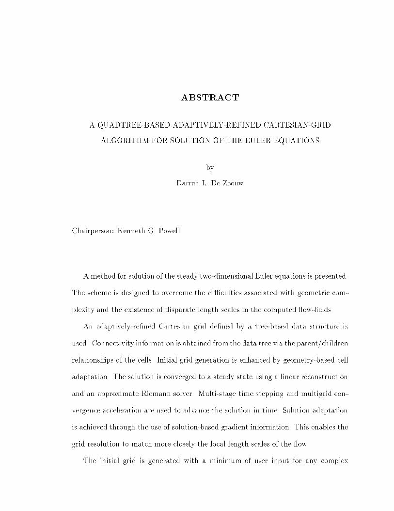
ABSTRACTA QUADTREE-BASED ADAPTIVELY-REFINED CARTESIAN-GRIDALGORITHM FOR SOLUTION OF THE EULER EQUATIONSbyDarren L. De ZeeuwChairperson: Kenneth G. PowellA method for solution of the steady two-dimensional Euler equations is presented.The scheme is designed to overcome the di�culties associated with geometric com-plexity and the existence of disparate length scales in the computed ow-�elds.An adaptively-re�ned Cartesian grid de�ned by a tree-based data structure isused. Connectivity information is obtained from the data tree via the parent/childrenrelationships of the cells. Initial grid generation is enhanced by geometry-based celladaptation. The solution is converged to a steady state using a linear reconstructionand an approximate Riemann solver. Multi-stage time stepping and multigrid con-vergence acceleration are used to advance the solution in time. Solution adaptationis achieved through the use of solution-based gradient information. This enables thegrid resolution to match more closely the local length scales of the ow.The initial grid is generated with a minimum of user input for any complex

1con�guration. The user need only specify a set of points de�ning the bodies, thebase grid resolution, and cell size thresholds for the geometry-based adaptation.With proper thresholds, the grid is automatically adapted to the curvature of abody, providing the resolution required to resolve that body adequately. The grid isthen improved through the use of solution-based adaptation.The di�culties associated with the small cut cells created by the arbitrary waythat the Cartesian grid cuts through the body are overcome by using local time-stepping, coupled with a linear reconstruction method designed speci�cally for un-structured grids.The solutions obtained show the second-order global accuracy of the scheme. Re-sults are presented for airfoils at subsonic, transonic, and supersonic speeds. Theresults compare favorably with benchmark solutions on structured grids with sub-stantially more cells. Also included are a channel ow, several axisymetric jet ows,and several multi-element airfoil ows. In all cases, the small cut cells generated bythe intersection of the body with the Cartesian grid have no adverse e�ect on thesmoothness of the solution. The broad range of results presented demonstrates thegeometric exibility of this approach, as well as the accuracy and e�ciency attainableby solution-based adaptation.