XIV CONFERENZA IL FUTURO DEI SISTEMI DI WELFARE NAZIONALI TRA INTEGRAZIONE EUROPEA E DECENTRAMENTO REGIONALE coordinamento, competizione, mobilità Pavia, Università, 4 - 5 ottobre 2002 QUALITY AND ADVERTISING IN A DYNAMIC MONOPOLY LUCA COLOMBO pubblicazione internet realizzata con contributo della società italiana di economia pubblica dipartimento di economia pubblica e territoriale – università di Pavia
Transcript
XIV
C
ON
FE
RE
NZ
A IL FUTURO DEI SISTEMI DI
WELFARE NAZIONALI TRA INTEGRAZIONE EUROPEA E DECENTRAMENTO REGIONALE
coordinamento, competizione, mobilità
Pavia, Università, 4 - 5 ottobre 2002
QUALITY AND ADVERTISING IN A DYNAMIC MONOPOLY
LUCA COLOMBO
pubblicazione internet realizzata con contributo della
società italiana di economia pubblica
dipartimento di economia pubblica e territoriale – università di Pavia
Quality and Advertising in a Dynamic Monopoly¤
Luca ColomboDepartment of Economics
University of BolognaStrada Maggiore 45, 40125 Bologna, Italy
I apply optimal control theory to analyze a dynamic setting where a ver-tically di¤erentiated monopolist, through capital accumulation over time, mayinvest both in product quality and advertising campaigns. By comparing themonopolist’s behavior to the social planner’s, I show that, at the steady state:(i) the monopolist’s bi-dimensional R&D portfolio is always distorted, along,at least, one dimension; (ii) the level of demand induced by the monopolistexactly coincides with the one a benevolent social planner would choose. Thelatter result is illustrated within a linear-quadratic technology.
Keywords: product quality, advertising, dynamic monopoly, vertical dif-ferentiation, capital accumulation.
JEL Classi…cation: D3, L12, O31.
¤I am grateful to Luca Lambertini for his guidance throughout the paper’s evolution. Anyremaining errors, of course, are my own.
1382
1 IntroductionThe existing literature on advertising dynamic models can essentially be partitionedinto two main subsets (see Sethi, 1977). The …rst, à la Nerlove and Arrow (1962),considers advertising as an instrument to increase the stock of goodwill or reputation;the second, à la Vidale and Wolfe (1957), is characterized by a direct relationshipbetween advertising expenditures and the rate of change in sales1 .
With regard to product quality provision, a dynamic set-up has prevalently beenadopted in relation with advertising expenditures aimed at the formation of goodwill(see Kotowitz and Mathewson, 1979; Conrad, 1985; Ringbeck, 1985)2. A prominentexception is represented by Lambertini (2001), who investigates a di¤erential duopolygame where …rms supply goods of di¤erent quality, resulting from capital accumula-tion over time. The set-up is borrowed from static monopolistic models with verticaldi¤erentiation (see Spence, 1975; Mussa and Rosen, 1978). The basic insight commonto these contributions is that a private monopolist designs the product to match thepreference of the marginal consumer, while a benevolent social planner cares aboutthe taste of the average one. Therefore, quality overprovision (underprovision) ariseswhenever the marginal willingness to pay of the latter results lower (higher) than theformer’s. In another paper, Lambertini (1997) shows that under largely acceptablehypothesis concerning the distribution of the population3 and a well behaving costfunction4, quality distortions do not arise, while prices and quantities are upwardsand downwards distorted, respectively. At a …rst glance, this result seems to be incontrast with the conventional wisdom on quality provision by a vertically di¤erenti-ated monopolist (Spence, 1975). Actually, what Spence argues is that for given andequal output, compared to the social planning, the monopolist undersupplies productquality5 (see Tirole, 1988). However, prices distortions are quite likely to happenin monopoly, not to use the term always. Consequently, one could be tempted toask himself whether Spence’s arguments are wrong. As Tirole (1988) well explains,when the monopoly structure is not questioned, reasoning for given quantities can beappropriate. But if the purpose of the analysis is to compare the monopoly to thesocial planning, such a reasoning is not acceptable, since it does not allow to takeinto account the global dead weight loss. Therefore, as usual, all depends on whatone is interested in.
1For surveys, see JÁrgensen (1982), Feichtinger, Hartl and Sethi (1994) and Dockner, JÁrgensen,Van Long and Sorger (2000, ch.11)
2For surveys on dynamic advertising, see Sethi (1977); JÁrgensen (1982); Feichtinger andJÁrgensen (1983); Erickson (1991); Feichtinger, Hartl and Sethi (1994).
3An uniform density function is assumed.4The total cost function is C (x; q); with Cx > 0; Cq > 0; Cxx ¸ 0; Cqq ¸ 0; x and q being
quantity and quality, respectively.5A su¢cient condition for this to happen is that the marginal willingness to pay for quality
decreases with the quantity purchased, i.e., marginal and absolute willingness to pay for quality bepositively linked.
1383
I apply optimal control theory6 to analyze a dynamic setting where a verticallydi¤erentiated monopolist, through capital accumulation over time, may invest bothin product quality and advertising campaigns7. The …rst task of the analysis is tocompare the monopolist’s bi-dimensional R&D portfolio with the social optimum.To this aim, I start by applying a very general model where functional speci…cationsare avoided. I solve both the monopolist and the social planner’s problem for theimplicit quality and advertising steady state levels, as well as for the related invest-ments. Then, by comparing the implicit solutions, I conclude that the monopolist’sbi-dimensional R&D portfolio is always distorted, along, at least, one dimension.
The reminder of this paper is structured as follows. The general model is laid outin section 2. In section 3, I focus on product quality investments, while in section 4,I focus on advertising campaigns. In section 5, aimed at obtaining explicit solutions,I employ a linear-quadratic technology, showing that, when both investments arejointly activated, a pro…t-maximizing monopolist provides the market with the …rstbest quantity level. In section 6, I evaluate the resulting monopolist’s equilibriain terms of welfare, suggesting which should be the optimal policies to cope withdynamic ine¢ciencies. Finally, in section 7, I provide concluding remarks.
2 The modelI consider a market for vertically di¤erentiated products where a monopolist subjectto no entry threat supplies a single variety q at price p in a number of units x anda¤ects market preferences by means of advertising campaigns. Consumers are orderedalong a support S = µ1¡ µ0 on the basis of their quality appraisal, expressed by theirmarginal willingness to pay, µ. Without any loss of generality, let S be unitary, withµ1 > 1. The population is distributed according to the density f(µ): Suppose f(µ)be uniform. Since µi is the marginal willingness to pay characterizing consumer i, hisgross surplus from the consumption of quality q is given by:
V (µi; q) = µiq (1)
Net surplus simply amounts to:
S(µi; q; p) = µiq ¡ p (2)
Each consumer is confronted with the choice between buying or not buying one unitof a certain variety. These alternatives are equivalent if:
0 = µiq ¡ p) µk =pq
(3)
6See Chiang, 1992 or Seierstad and Sydsaeter, 1987. The former provides a good introductionto optimal control theory, while the latter, at a less introductory level, is reached of economicapplications.
7The analysis of dynamic monopoly originates with Evans (1924) and Tintner (1937).
1384
Therefore, total demand writes:
x = µ1 ¡ µk = µ1 ¡ pq
· 1 (4)
Production entails a variable cost, which is assumed to be convex in the quality level:
C q = xq2 (5)
and the setup of advertising campaigns entails a …xed cost:
C µ1 = B + °2(µSS1 ¡ µ1)2 (6)
with µSS1 > µ1 and B; ° > 0; where µSS1 denotes the exogenous advertising target, ° isa parameter weighing the square of the distance between such a target and the actualreservation price, and B is the amount of money to be spent in the case in which thetarget is achieved.
Instantaneous pro…ts amount to:
¦ = (p ¡ q2)(µ1 ¡ pq) ¡B ¡ °
2(µSS1 ¡ µ1)2 (7)
Instantaneous consumer surplus is:
CS =µ1Z
µk
(µq ¡ p)dµ = 12µ21q2 ¡ 2pµ1q + p2
q(8)
Instantaneous social welfare is obtained adding up consumer surplus and pro…ts:
W = ¦+CS (9)
Now, let me introduce the time dimension into this setup. Suppose, …rst, thatthe market exists over t 2 [0;1): To keep things manageable, I assume that both thesize and the distribution of the population remain constant over t. Accordingly, thedemand function can be written:
x(t) = µ1(t) ¡ p(t)q(t)
· 1 (10)
In the remainder, I will consider the three following scenarios: (i) investments inproduct quality; (ii) investments in advertising campaigns; (iii) both jointly.
In (i), while µ1(t) remains constant at bµ1; in response of capital accumulation overtime, q(t) evolves according to the following kinematic:
@q(t)@t
= bÁ(k(t))¡ ±q(t) (11)
1385
In (ii), while q(t) remains constant at bq, in response of capital accumulation overtime, µ1(t) evolves according to the following kinematic:
@µ1(t)@t
= cÃ(l(t))¡ ±µ1(t) (12)
where k(t) and l(t) denote the speci…c capital to be devoted to product quality im-provements and advertising campaigns, respectively; Á(k) and Ã(l) are di¤erentiable
and invertible functions de…ned in the set of real numbers, with@Á(k)@k
> 0;@Ã(l)@l> 0;
@Á2(k)@2k
· 0; @Ã2(l)@2l
· 0: ± 2 [0; 1] is the usual depreciation rate, supposed to be com-mon to both dynamics for the sake of simplicity. Finally, b and c are positive realconstants.
Let r > 0 be the price for k(t) and w > 0 be the price for l(t). Therefore,instantaneous investments costs in quality improvements and advertising campaignsare, respectively:
IC q(t) = rh(k(t)) (13)
ICµ1(t) = wz(l(t)) (14)
with@h(k(t))@k(t)
> 0;@2h(k(t))@k(t)2
¸ 0;@z(l(t))@l(t)
> 0;@2z(l(t))@l(t)2
¸ 0:
3 Product Quality
3.1 The Social Planner’s equilibriumThe current value Hamiltonian for the social planner’s problem (P ) turns out to be:
H = e¡½t
8<:
12( bµ1)2q2 ¡ 2pbµ1q + p2
q+ (p¡ q2)(bµ1 ¡ p
q)+
¡rh(k(t)) + ¸1(t)(bÁ(k(t))¡ ±q(t))
9=; (15)
where ¸1(t) = ¹1(t)e½t , ¹1(t)being the co-state variable associated to q(t): Thefeasible set is zP = fbµ1 ¸ q; p ¸ 0; q ¸ 0;
pq
¸ µ0g: To simplify notations, I neglect
the index of time. By applying Pontryagin’s maximum principle, necessary conditionsfor a path to be optimal are8 :
Hp = 0 ! p = q2 (16)
Hk = 0 !r@h(k)@k¸1b
=@Á(k)@k
! ¸1 =r@h(k)@k
b@Á(k)@k
(17)
8For a revision of the methodology have a look at Chiang’s book (1992).
1386
Hq = ¡12
¡( bµ1)2q2 ¡ p2+ 4q3 bµ1 ¡ 2q2pq2
¡ ¸1± = ½¸1¡¢¸1 (18)
along with the transversality condition:
limt!1¹1q = 0 (19)
I apply Mangasarian’s theorem to check whether these conditions are also su¢cient:
de…ne V P =(bµ1)2q2 ¡ p2 ¡ 2q3 bµ1 + 2q2p
2q¡ rh(k); v1 = bÁ(k(t)) ¡ ±q(t): I compute:
@2V P
@2q= ¡2µ1 ¡ p
2
q3< 0 always;
@2V P
@2p= ¡1q< 0 always. Then I compute:
@2v1@2q
= 0;
@2v1@2k
= b@2Á(k)@2k
· 0, as long as b > 0 and@2Á(k)@2k
· 0, which is always true byassumption. It remains to check that, in the optimal solution, the co-state variable be
non negative: ¸1 =r@h(k)@k
b@Á(k)@k
¸ 0 by assumption. Therefore, the necessary conditions
of the maximum principle are also su¢cient.By di¤erentiating (17) w.r.t. time:
¢¸1=
r¢k [@2h@2k@Á@k
¡ @h@k@2Á@2k
]
b[@Á@k
]2(20)
By inserting (20), (16) and (17) into (18) and by solving for¢k:
¢k=
0B@¡(bµ1)2
2+ 2q bµ1 ¡ 3
2q2 +
r@h(k)@k
b@Á(k)@k
(± + ½)
1CA
b(@Á@k )
2
rµ@2h@2k@Á@k
¡ @h@k@2Á@2k
¶ (21)
with@2h(k)@2k
@Á(k)@k
6= @h(k)@k@2Á(k)@2k
, i.e., the ratio between second derivatives has to
be di¤erent from the corresponding ratio between …rst derivatives. Since@2h@2k@Á@k>
@h@k@2Á@2k
:
sign(¢k) = sign(
(4qµ1 ¡ µ21 ¡ 3q2)2
+r(± + ½)b
(k))
Therefore, with q < 13µ1 (see …gure 1) if q increases k does likewise9.
9 If q > 23µ1 the opposite holds. However, since the locus
¢q= 0 is represented by a function whichis monotonically decreasing, q > 1
3 µ1 can not be an equilibrium.
1387
The steady state conditions¢k= 0;
¢q= 0 imply:
¢k= 0 ! @Á(k)
@k= 2r
@h(k)@k
± + ½
b³¡4bµ1q +3q2+ ( bµ1)2
´ (22)
¢q= 0 ! q =bÁ(k)±
(23)
By solving (22) for q I …nd the following roots:
q1;2 =23
bµ1 § 13b
qb2(bµ1)2 +6r(± + ½)¢(k) (24)
where¢(k) =
@h(k)@k@Á(k)@k
, with¢(k)0 = h00Á0 ¡ h0Á00(Á0)2
> 0 since h00 > 0; Á0 > 0; h0 > 0; Á00 ·
0 by assumption. Since q01;2 = §(¡ 13b
12 (µ
2b2 + 12br(± + ½)¢)¡1=212br(± + ½)¢0) ? 0;
the root q1 = 23bµ1 + 1
3b
qb2(bµ1) + 6r(± + ½)¢(k) is not admissible, being q1 > bµ1 for
any k > 010. What about concavity? It is easy to verify that q002 > 0 if ¢00 < 0: Asu¢cient condition for ¢00 < 0 to hold follows:
Á0
2Á00h000Á0 ¡ h0Á000h00Á0 ¡ h0Á00 > 1
Notice that when h000 and Á000 are nil the condition does not hold but this does notimply that q 00 < 0. The necessary condition for q 00 > 0 turns out to be:
¢00
¢0 <6br(± + ½)¢0
µ2b+ 12r(± + ½)¢
Let me assume that the above disequality holds along the entire admissible range ofk, implying that q 002 > 0: Anyway, the qualitative analysis of the equilibrium is nota¤ected by the concavity of the locus
¢q= 0, even in the case in which the sign of thesecon derivative changes within the admissible range of k.
I am interested in investigating the dynamics of the system in the positive quad-rant of the space fk; qg, which is described in …gure 1 (see the Appendix). The locus¢k= 0 corresponds to the decreasing curve which intersects the vertical axe at q =
bµ13 .
The economic interpretation of such a locus is easy. When q is high, the planneris willing to stop the accumulation process quickly, at a low level of k. Viceversa,when q is low, he has incentives to keep on accumulating until the optimal level ofq is reached. Moving from the origin, the locus
¢q= 0 draws a curve which with no10q belongs to the feasible set as long as it is not greater than µ1.
1388
doubt intersects the locus¢k= 0 once. The planner’s equilibrium is denoted with a
P: Clearly, it is a saddle and it can be approached only along the north-west armof the path. As usual, the initial conditions play a crucial role in determining thetrajectory of both variables over time. By following the directions indicated by the
arrows, if q(0) <bµ13
the steady state can never be achieved. Similarly, if q(0) >>bµ13
,
the descending trajectory crosses the locus¢q= 0 at the right of P and then becomes
increasing.With regard to the formal stability analysis, let me focus on the following inter-
esting case: ¢(k) = Á(k) = k. This, among others, is the case of a linear quadratictechnology. The resulting dynamic system described by (11) and (21) can be writtenin matrix form as follows:
" ¢q¢k
#=
" ¡± bbr(2µ1 ¡ 3
2q) ± + ½
# ·qk
¸+
"0
¡ b2rµ21
#
Since the determinant of the above 2 £ 2 matrix is always negative in the relevantparameter range, the equilibrium is stable along a saddle path.
3.2 The Monopolist’s equilibriumThe current value Hamiltonian for the monopolist’s problem (M) turns out to be:
where ¸1(t) = ¹1(t)e½t , ¹1(t) being the co-state variable associated to q(t). Thefeasible set is zM = fq · bµ1; q ¸ p
bµ1; p ¸ q2; p
q¸ µ0g: To simplify notations, as
before, I neglect the index of time. By applying Pontryagin’s maximum principle,necessary conditions for a path to be optimal are:
Hp = 0 ! p = q(bµ1 + q)2
! xM =bµ1 ¡ q2
(26)
Hk = 0 !r@h(k)@k¸1b
=@Á(k)@k
! ¸1 =r@h(k)@k
b@Á(k)@k
(27)
Hq = ¡2q bµ1 +p2
q2+ p¡ ¸1± = ½¸1¡
¢¸1 (28)
along with the transversality conditions:
limt!1¹1q = 0 (29)
1389
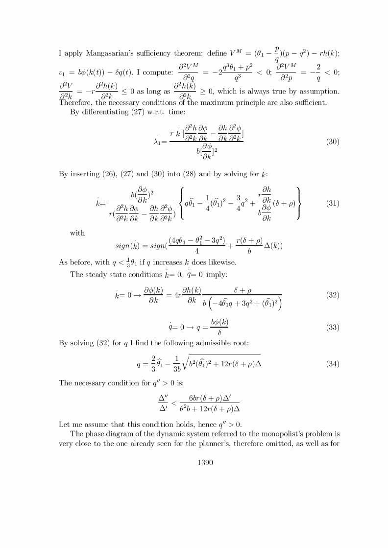
I apply Mangasarian’s su¢ciency theorem: de…ne V M = (µ1 ¡ pq)(p ¡ q2) ¡ rh(k);
v1 = bÁ(k(t)) ¡ ±q(t): I compute:@2V M
@2q= ¡2
q3µ1 + p2
q3< 0;
@2V M
@2p= ¡2
q< 0;
@2V@2k
= ¡r@2h(k)@2k
· 0 as long as@2h(k)@2k
¸ 0, which is always true by assumption.Therefore, the necessary conditions of the maximum principle are also su¢cient.
By di¤erentiating (27) w.r.t. time:
¢¸1=
r¢k [@2h@2k@Á@k
¡ @h@k@2Á@2k
]
b[@Á@k
]2(30)
By inserting (26), (27) and (30) into (28) and by solving for¢k:
¢k=
b(@Á@k
)2
r(@2h@2k@Á@k ¡ @h@k
@2Á@2k )
8><>:q bµ1 ¡ 1
4( bµ1)2 ¡ 3
4q2 +
r@h@k
b@Á@k
(± + ½)
9>=>;
(31)
with
sign(¢k) = sign(
(4qµ1 ¡ µ21 ¡ 3q2)4
+r(± + ½)b
¢(k))
As before, with q < 13µ1 if q increases k does likewise.
The steady state conditions¢k= 0;
¢q= 0 imply:
¢k= 0 ! @Á(k)
@k= 4r@h(k)
@k± + ½
b³¡4bµ1q +3q2+ ( bµ1)2
´ (32)
¢q= 0 ! q =bÁ(k)±
(33)
By solving (32) for q I …nd the following admissible root:
q =23
bµ1 ¡ 13b
qb2( bµ1)2 + 12r(± + ½)¢ (34)
The necessary condition for q 00 > 0 is:
¢00
¢0 <6br(± + ½)¢0
µ2b+ 12r(± + ½)¢
Let me assume that this condition holds, hence q 00 > 0:The phase diagram of the dynamic system referred to the monopolist’s problem is
very close to the one already seen for the planner’s, therefore omitted, as well as for
1390
the stability analysis. What is relevant to my purpose is to compare (34) with (24)in order to understand who between the monopolist and the planner invests morein product quality. (34) and (24) are two descending curves with common intercept,but di¤erent slopes. It is straightforward to assess that the curve which is referred tothe monopolist’s problem is always less-sloped than the one referred to the planner’s.Since the locus
¢q= 0 is common to both, it follows that the monopolist ends up withundersupplying product quality. Figure 2 (see the Appendix) illustrates the previousdiscussion.
Proposition 1 For any given bµ1, the monopolist underinvests in product quality com-pared with the social optimum. If q(0) 2 ( bµ1=3; q0) with q0 su¢ciently low, the result-ing equilibria are stable along a saddle path.
It is worth noting that, in order to have the monopolist producing the level ofproduct quality which is socially desirable, the monopolist should face a richer marketthan the planner: the locus
¢k= 0 referred to the his problem should shift upwards so
as to cross the locus¢k= 0 referred to the planner’s exactly at P .
4 Advertising Campaigns
4.1 The Social Planner’s equilibriumThe current value Hamiltonian for the social planner’s problem (P ) turns out to be:
I apply Mangasarian’s theorem to check whether these conditions are also su¢-
cient: de…ne V P =( bµ1)2q2 ¡ p2 ¡ 2q3 bµ1 +2q2p
2q¡ Cµ1 ¡ wz(l); v2 = cÃ(l(t))¡ ±µ1(t):
I compute: @2V P
@2µ1= q ¡ ° · 0 as long as ° ¸ q: Then I compute: @
2v2@2µ1
= 0;
@2v2@2l
= c@2Ã(l)@2l
· 0, as long as c > 0 and @2Ã(l)@2l
· 0, which is always true by
assumption;@2V@2p
= ¡2q< 0;
@2V@2l
= ¡w@2z(l)@2l
· 0 as long as@2z(l)@2l
¸ 0, which
is always true by assumption.It remains to check that, in the optimal solution, the
co-state variable be non negative: ¸2 =w@z(l)@l
c@Ã(l)@l
¸ 0 by assumption.Therefore, as
long as ° ¸ q, the necessary conditions of the maximum principle are also su¢cient.By di¤erentiating (37) w.r.t. time:
¢¸2=
w¢l [@2z@2l@Ã@l
¡ @z@l@2Ã@2l
]
c[@Ã@l
]2(40)
By inserting (37) and (40) into (38) and by solving for¢l I obtain:
¢l=
³¡µ1bq + bq2 + °(µ1 ¡ µSS1 ) +
wc(± + ½)¯(l)
´ c(@Ã@l
)2
w(@2z@2l@Ã@l ¡ @z@l
@2Ã@2l )
(41)
with ¯(l) = z0=Ã0; ¯(l)0 = z00Ã0 ¡ z0Ã00(Ã0)2
> 0: ¯(l)00 > 0 if z000Ã0 > z0Ã000: Since @2z@2l@Ã@l>
@z@l@2Ã@2l
:
sign(¢l) = sign(¡µ1bq + bq2 + °(µ1 ¡ µSS1 ) + w
c(± + ½)¯(l))
>From s.o.c., ° > q, so if µ1 increases l does likewise.The steady state condition
¢l= 0 implies:
@Ã@l
= w@z@l
± + ½c(bq (µ1 ¡ bq)¡ °(µ1 ¡ µSS1 ))
(42)
which, under the assumption that at the steady state µ1 = µSS1 , yields:
µP1 = bq + w(± + ½)cbq ¯ ) xP = w± + ½cbq ¯ (43)
1392
If z000Ã0 > z0Ã000, then ¯ 00 > 0 and µ00 > 0: For the time being, suppose this is the case.The steady state condition
¢µ1= 0 implies:
¢µ1= 0 ! µ1 =
cÃ(l)±
(44)
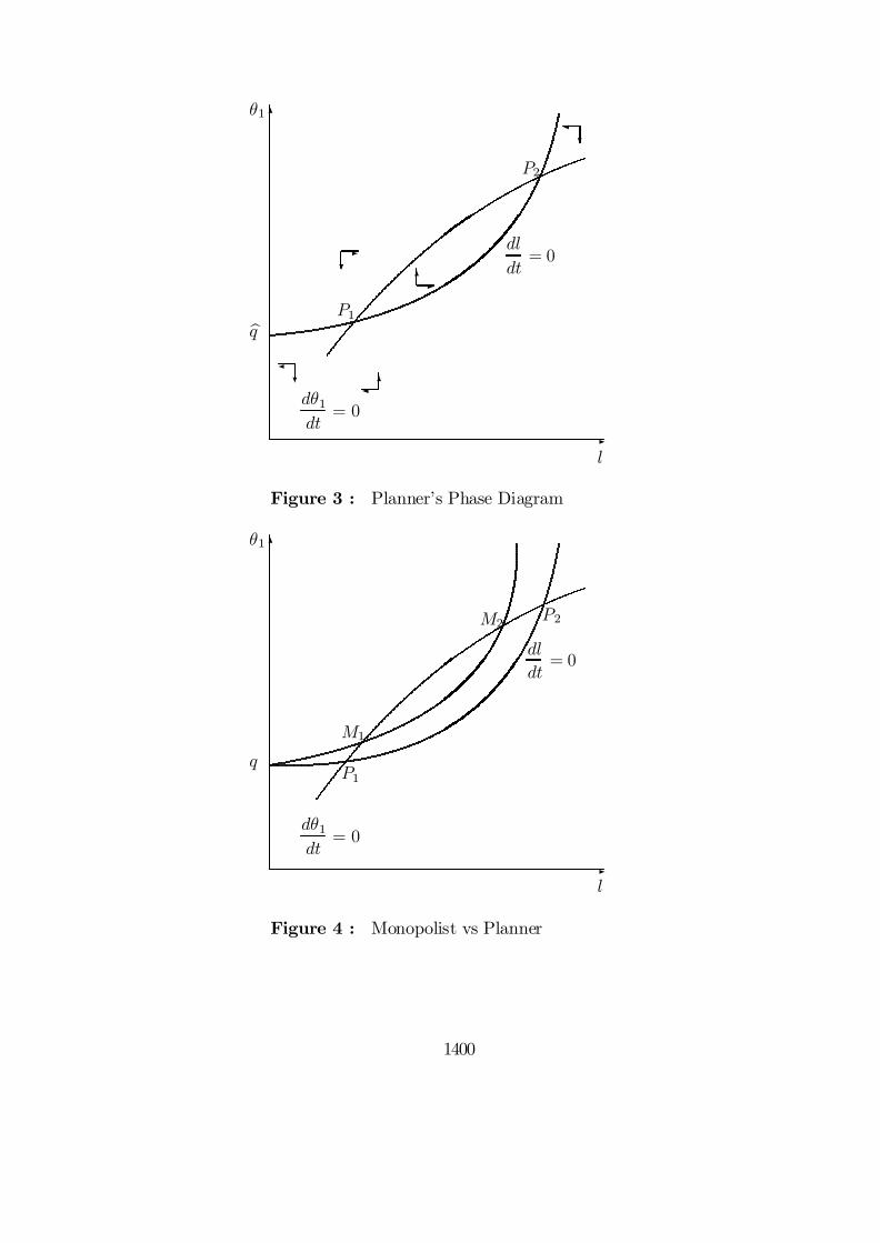
I am interested in investigating the dynamics of the system in the positive quad-rant of the space fl; µ1g, which is described in …gure 3 (see the Appendix). The locus¢l= 0 corresponds to the increasing curve that intersects the vertical axe at µ1 = bq.Moving from the origin, the locus
¢µ1= 0 draws a curve that may or may not intersect
the locus¢l= 0. In the case depicted in …gure 3, two equilibria arise: P1 which is a
saddle, and P2 which is a stable equilibrium. Su¢cient but not necessary conditionsto have equilibrium unicity are: Ã00 = 0 and µ001 · 0.
As a mere illustration of the stability analysis, I focus on the following simple case:¯(l) = Ã(l) = l. This is, among others, the case of a linear quadratic technology, inwhich only one equilibrium arises. From (12) and (41), the dynamic system can bewritten in matrix form:
" ¢µ1¢l
#=
"¡± c
cw(¡bq + °) ± + ½
# ·µ1l
¸+
"0
cw(q2 ¡ °µSS1 )
#
Since the determinant of the above 2 £ 2 matrix is always negative in the relevantparameter range, the equilibrium is stable along a saddle path.
4.2 The Monopolist’s equilibriumThe current value Hamiltonian for the monopolist’s problem (M) turns out to be:
H = e¡½t
8<:
(µ1(t) ¡ p(t)bq )(p(t) ¡ bq2)¡B ¡ °2(µSS1 ¡ µ1)2+
¡wz(l(t)) + ¸2(t)(cÃ(l(t)) ¡ ±µ1(t))
9=; (45)
where ¸2(t) = ¹2(t)e½t , ¹2(t)being the co-state variable associated to µ1(t): Thefeasible set is zM = fµ1 ¸ q; q ¸ p
µ1; p ¸ q2; pq ¸ µ0g: To simplify notations, I
neglect the index of time. By applying Pontryagin’s maximum principle, necessaryconditions for a path to be optimal are:
Hp = 0 ! p = bq(µ1 + bq)2
! xM =µ1 ¡ bq
2(46)
Hl = 0 !w@z(k)@l¸2c
=@Ã(l)@l
! ¸2 =w@z(l)@l
c@Ã(l)@l
(47)
1393
Hµ1 = p¡ bq2 ¡ °(µ1 ¡ µSS1 ) ¡ ¸2± = ½¸2¡¢¸2 (48)
along with the transversality conditions:
limt!1¹2µ1 = 0 (49)
I apply Mangasarian’s su¢ciency theorem: de…ne V M = (µ1¡pq)(p¡q2)¡Cµ1¡wz(l);
v2 = cÃ(l(t)) ¡ ±µ1(t): I compute: @2V M
@2µ1= ¡° · 0 as long as ° ¸ 0; which is
always true by assumption; @2V@2p
= ¡2q< 0; @
2V@2l
= ¡w@2z(l)@2l
· 0 as long as
@2z(l)@2l
¸ 0, which is always true by assumption. Therefore, the necessary conditionsof the maximum principle are also su¢cient.
By di¤erentiating (47) w.r.t. time:
¢¸2=
w¢l [@2z@2l@Ã@l
¡ @z@l@2Ã@2l
]
c[@Ã@l
]2(50)
Similarly, by inserting (46), (47) and (50) into (48) and by solving for l I obtain:
¢l=
c[@Ã@l
]2
w(@2z@2l@Ã@l
¡ @z@l@2Ã@2l
)
8><>:
¡12µ1bq +
12bq2+ °(µ1 ¡ µSS1 ) +
w@z@l
c@Ã@l
(± + ½)
9>=>;
(51)
with @2z(l)@2l
@Ã(k)@k
6= @h(l)@l@2Ã(l)@2l
, i.e., the ratio between second derivatives has tobe di¤erent from the corresponding ratio between …rst derivatives.
sign(¢l) = sign(¡
12µ1bq +
12bq2 + °(µ1 ¡ µSS1 ) +
wc(± + ½)¯(l))
As before, given s.o.c., if µ1 increases l does likewise.The steady state condition
¢l= 0 implies:
@Ã@l
= 2w@z@l
± + ½c(bq (µ1 ¡ bq)¡ 2°(µ1 ¡ µSS1 ))
(52)
By solving (53) for µM1 :
µM1 = bq + 2w(± + ½)cbq ¯ ) xM = w
± + ½cbq ¯ (53)
1394
It is worth noting that xM = xP as long as lM = lP , that is, as long as the monopolist’sadvertising investment coincide with the planner’s.
Assume z000Ã0 > z0Ã000, implying that µ00 > 0:As before, the steady state condition
¢µ1= 0 implies:
¢µ1= 0 ! µ1 =
cÃ(l)±
(54)
By looking at …gure 4 (see the Appendix) it is possible to make a direct comparisonbetween the monopolist’s problem and the planner’s in the case in which µ00 > 0. Theabove discussion can be summarized by the following:
Proposition 2 In all odd (even) equilibria the monopolist overinvests (underinvests)in advertising compared with the social optimum. As a consequence, in all odd (even)equilibria the monopolist oversupplies (undersupplies) the good. If the monopolist’sadvertising investments and the planner’s coincide, then the monopolist ends up withproviding the market with the …rst best quantity level.
5 Product Quality and Advertising Campaigns
Let Á(k) = k; Ã(l) = l and h(k) =k2
2 ; z(l) =l2
2 throughout this section; this implies:¢(k) = k; ¯(l) = l: More generally, let Á(k) = ¢(k) and Ã(l) = ¯(l).
5.1 The social planner’s equilibriumThe Hamiltonian function the social planner faces is:
H = e¡½t
8><>:
µ21q2 ¡ 2pµ1q + p2
2q+ (p¡ q2)(µ1 ¡ p
q)¡B ¡ °(µSS1 ¡ µ1)2+
¡rk(t)2
2¡ wz(t)
2
2+ ¸1(t)(bk(t) ¡ ±q(t)) + ¸2(t)(cl(t) ¡ ±µ1(t))
9>=>;
(55)
where ¸1(t) = ¹1(t)e½t , ¹1(t) being the co-state variable associated to q(t); ¸2(t) =¹2(t)e½t , ¹2(t) being the co-state variable associated to µ1(t): By using (21) and (41)the following dynamics obtain:
@k@t
= k(½ + ±) +br4qµ1 ¡ µ21 ¡ 3q2
2(56)
@l@t
= l(½ + ±) +cw(q(q ¡ µ1) + °(µ1 ¡ µSS1 )) (57)
1395
The dynamic system (57) and (58) along with the equations of motion (11) and (12)yields the following steady states11 :
µPSS1 =9: 90372b2
r± (± + a) (58)
qPSS =2: 78082b2
r± (± + a) (59)
xPSS =3: 561 4b2
r± (± + a) (60)
5.2 The monopolist’s equilibriumThe Hamiltonian function the monopolist faces is:
H = e¡½t
8><>:
(p¡ q2)(µ1 ¡ pq)¡B ¡ °(µSS1 ¡ µ1)2+
¡rk(t)2
2¡ wz(t)
2
2+ ¸1(t)(bk(t) ¡ ±q(t)) + ¸2(t)(cl(t) ¡ ±µ1(t))
9>=>;
(61)
where ¸1(t) = ¹1(t)e½t , ¹1(t) being the co-state variable associated to q(t); ¸2(t) =¹2(t)e½t , ¹2(t)being the co-state variable associated to µ1(t): To ease notations, Idrop the indication of time. By using (27) and (51), the following dynamic systemobtains:
@k@t
= k(½ + ±) +br4qµ1 ¡ µ21 ¡ 3q2
4(62)
@l@t
= l(½+ ±) +cwq(q ¡ µ1) + 2(°(µ1 ¡ µSS1 )
2(63)
The above system along with the equations of motion (11) and (12) yields:
µMSS1 =9: 903 7b2
r± (± + a) (64)
qMSS =2: 780 8b2
r± (± + a) (65)
xMSS =3: 5614b2
r± (± + a) (66)
with b > 1: 887 2pr± (± + a) for x < 1:
Proposition 3 Within a linear quadratic technology, the monopolist invests both inproduct quality and advertising campaigns twice as much compared to the social plan-ner. As a consequence, he provides the market with the …rst best quantity level.
11To ease calculations I assume that b = c and r = w.
1396
6 Policy implicationsThe task of this section is to make explicit the properties of the linear quadratictechnology in terms of welfare and discuss them from a policy perspective. The focusis on e¢ciency. Before proceeding, let me remind you that, at the steady state,welfare is simply given by the sum between consumers surplus and pro…ts steadystate values, as follows:
WMSS = CSMSS + ¼MSS (67)First, I compute the level of welfare at the steady state under monopoly regime. Byapplying (14) and (10), respectively, and by taking into account that, at the steadystate, capital accumulation stops:
WMSS = r2±2 (± + a)280:44 7r±(± + a)¡ 9: 9036b2
b6¡B (68)
where
CSMSS = 14((µMSS1 )2
2qMSS ¡ µMSS1 (qMSS)2 + (qMSS)3
2)
=17: 636b6r3±3 (± + a)3 (69)
¼MSS = 0:0024759r2±2 (± + a)225369r±(± + a) ¡ 4000b2
b6¡B (70)
with B small enough to respect the usual non negative constraints and b < 2:8501
pr± (± + a) for WMSS to be positive.
The corresponding computation under social planning is omitted, since it is notpossible to compare the welfare arising from markets in which the intercept term ofthe demand functions di¤ers, as it is in our case. Rather, I focus onWMSS , aimed atinvestigating which are its responses to di¤erent policy regulations. Assume that thegovernment may choose between two kinds of policies: (i) to a¤ect the instantaneousinvestment costs, through r; (ii) to a¤ect the accumulation process, through b. Noticethat, in order to obtain manageable solutions, I have assumed that c = b and w = r:As a consequence, b enters the accumulation of both quality and reservation price,while r denotes the price of both speci…c inputs, k and l. Consider, …rst, policy (i).Its e¤ect is given by:
@WMSS
@r = 232 533 (± + ½)3 r2±3
b6 > 0 (71)
Therefore, a marginal increase in r yields welfare improvements, since it hinders theacquisition of capital.
As to policy (ii), its e¤ect is given by:
@WMSS
@b= ¡465 066 (± + ½)3 r3
±3
b7< 0 (72)
1397
Therefore, a marginal decrease in b yields welfare improvements, since it slows downthe accumulation of capital.
In order to understand which of the two policies should be preferred, I considerthe following equation: ¯̄
¯̄@WMSS@b
¯̄¯̄ = 2r
b
¯̄¯̄@WMSS@r
¯̄¯̄ (73)
It is immediate to draw from it:
Proposition 4 As long as input prices are su¢ciently high, r >b2, it is optimal
to reduce the accumulation of capital through the equations of motion, both w.r.t.consumers’surplus and pro…ts. This amounts to saying that regulation (ii) should bepreferred to regulation (i).
7 Concluding remarksThe comparison between static and dynamic ine¢ciencies which are due to a monop-olistic structure dates back to Schumpeter (1942). In accordance with him, I haveshown that, when both product quality and advertising investments are activated, amonopolist is more innovator than a social planner. More surprisingly, I have shownthat his traditional tendency to undersupply quantities is not robust to a dynamicsetting. The basic implication of this result is that, in weighing the pros and cons ofa monopolistic structure, one should be aware of making explicit the time horizon atwhich he refers itself. Indeed, quantity distortions are present in the short run, as weknow from static analyses, but they vanish in the long run, within a linear-quadratictechnology, at least. Further developments are needed to understand the extent towhich a vertical di¤erentiated monopolist may provide the market with the …rst bestquantity level, a result which, per se, deserves some attentions. As to product qualityprovision, the existing literature dealing with static models has not reached homoge-nous results, while dynamic analyses have been almost completely absconding. Theresult I have obtained is that, for any given reservation price, the monopolist alwaysunderinvests compared to the social planner. In my paper, I have also studied theappropriate policy implications w.r.t. the investments in R&D jointly considered: fora relatively low level of input prices, I have shown that it is optimal for the govern-ment increasing them up to a critical threshold, above which it becomes optimal toslow down the accumulation of capital.
1398
8 Graphical Appendix
Figure 1 : Planner’s Phase Diagram
6
-
-6¾?
¾6
-?
k
q
P
µ13
dqdt
= 0
dkdt
= 0
Figure 2 : Monopolist vs Planner
6
-
k
q
P
M
µ13
dqdt
= 0
dkdt = 0
1399
Figure 3 : Planner’s Phase Diagram
6
-
-6
¾?
¾?
¾¾6
-?
l
µ1
P1
P2
bq
dldt
= 0
dµ1dt
= 0
Figure 4 : Monopolist vs Planner
6
-l
µ1
M1
P1
M2 P2
q
dµ1dt
= 0
dldt
= 0
1400
References[1] Cellini, R. and L. Lambertini, 2002. Advertising in a di¤erential oligopoly game.
Journal of Optimization Theory and Applications. forthcoming.
[2] Chiang, A., 1992. Elements of dynamic optimization. New York, McGraw-Hill.
[3] Choi J.P., 1997. Herd behavior, the Penguin E¤ect, and the suppression of in-formational di¤usion: an analysis of informational externalities and payo¤ inter-dipendency. Rand Journal of Economics, 28 (3), 407-425.
[4] Conrad, K., 1985. Quality, advertising and the formation of goodwill under dy-namic conditions. in G. Feichtinger (ed), Optimal control theory and cconomicanalysis, vol.2, North-Holland, Amsterdam, 215-34.
[5] Dixit, A. and V. Norman, 1978. Advertising and welfare. Bell Journal of Eco-nomics, 9, 1-17.
[6] Dorfman, R. and Steiner, P.O., 1954. Optimal advertising and optimal quality.American Economic Review, 44, 826-836.
[7] Erickson, G.M., 1991. Dynamic models of advertising competition. Dordrecht,Kluwer.
[8] Evans, G.C., 1924. The dynamics of monopoly. American Mathematical Monthly,31, 75-83.
[9] Feichtinger, G., R.F. Hartl and P.S. Sethi, 1994. Dynamic optimal control modelsin advertising: recent developments. Management Science, 40, 195-226.
[10] Galbraith, J.K., 1967. The new industrial state. The New American Library,New York, ch.XVIII.
[11] JÁrgensen, S., 1982. A survey of some di¤erential games in advertising. Journalof Economics Dynamics and Control, 4, 341-69.
[12] Kotowitz, Y. and F. Mathewson, 1979. Advertising, consumer information, andproduct quality. Bell Journal of Economics, 10, 566-588.
[13] Lambertini, L., 1997. Does monopoly undersupply product quality?. Mimeo.
[14] Lambertini, L., 2001. Dynamic duopoly with vertical di¤erentiation. Mimeo.
[15] Mussa, M. and S. Rosen, 1978. Monopoly and product quality. Journal of Eco-nomic Theory, 18, 301-317.
[16] Nerlove, M. and Arrow, K.H., 1962. Optimal advertising policy under dynamicconditions, Economica, 124-142.
1401
[17] Schmalensee, R., 1978. A model of advertising and product quality. Journal ofPolitical Economy, 86, 1213-1225.
[18] Schmalensee, R, 1986. Advertising and market structure. in Stiglitz J. and F.Mathewson (ed), New Developments in the Analysis of Market Structure, MITPress, Cambridge, MA.
[19] Schumpeter, J.A., 1942. Capitalism, socialism and democracy. Harper, NewYork.
[20] Seierstad, A. and K. Sydsaeter, 1987. Optimal control theory with economicapplications. North-Holland.
[21] Sethi (1977), S.P., 1977. Dynamic optimal control models in advertising: a sur-vey. SIAM Review, 19, 685-725.
[22] Spence, A.M., 1975. Monopoly, quality, and regulation. Bell Journal of Eco-nomics, 6, 417-429.
[23] Vidale, M.L. and H.B. Wolfe, 1957. An operations research study of sales re-sponse to advertising. Operations Research, 5, 370-381.
[24] Tintner, G., 1937. Monopoly over time. Econometrica, 160-70.
[25] Tirole, J., 1988. The theory of industrial organization. MIT Press, Cambridge,MA.