Quality Assurance Project Plan

Puget Sound Dissolved Oxygen Modeling Study: Intermediate-scale Model Development April 2009 Publication No. 09-03-110

Publication and Contact Information This plan is available on the Department of Ecology’s website at www.ecy.wa.gov/biblio/0903110.html. Ecology’s Project Tracker Code for this study is 09-503-02. Waterbody Numbers: WA-PS-0010 through WA-PS-0300 (entire Puget Sound estuary system). For more information contact: Brandon Sackmann, Author Environmental Assessment Program Washington State Department of Ecology Olympia, Washington 98504-7710 Carol Norsen, Communications Consultant Phone: 360-407-7486

Washington State Department of Ecology - www.ecy.wa.gov/ o Headquarters, Olympia 360-407-6000 o Northwest Regional Office, Bellevue 425-649-7000 o Southwest Regional Office, Olympia 360-407-6300 o Central Regional Office, Yakima 509-575-2490 o Eastern Regional Office, Spokane 509-329-3400

Any use of product or firm names in this publication is for descriptive purposes only and does not imply endorsement by the author or the Department of Ecology.

If you need this publication in an alternate format, call Carol Norsen at 360-407-7486.

Persons with hearing loss can call 711 for Washington Relay Service. Persons with a speech disability can call 877- 833-6341.

Page 1

Quality Assurance Project Plan

Puget Sound Dissolved Oxygen Modeling Study:

Intermediate-scale Model Development

April 2009

Approved by:

Signature: Date: April 2009

Andrew Kolosseus, Client, Water Quality Program

Signature: Date: April 2009 Brandon Sackmann, principal Investigator and Author, SCS, EAP

Signature: Date: April 2009 Mindy Roberts, Project Manager, SCS, EAP

Signature: Date: April 2009 Karol Erickson, Author’s Unit Supervisor, SCS, EAP

Signature: Date: April 2009 Will Kendra, Author’s Section Manager, SCS, EAP

Signature: Date: April 2009 Robert F. Cusimano, Section Manager for Project Study Area, WOS, EAP

Signature: Date: April 2009 Bill Kammin, Ecology Quality Assurance Officer Signatures are not available on the Internet version. EAP – Environmental Assessment Program SCS – Statewide Coordination Section WOS – Western Operations Section

Page 2

Table of Contents

Abstract ................................................................................................................................4

Page

Background and Project Overview ......................................................................................5 Nutrient Pollution and Eutrophication ...........................................................................5 Eutrophication in Puget Sound ......................................................................................5 Project Description.........................................................................................................7 Project Goals and Objectives .........................................................................................8 Organization and Schedule ..........................................................................................10

Capabilities for a Dissolved Oxygen Model of Puget Sound ...........................................12 Hydrodynamics ............................................................................................................12 Water Quality ...............................................................................................................13 Ability to Incorporate Nearshore Processes at High Resolution .................................14 Summary ......................................................................................................................14

Recommendation for Model Selection and Model Approach ..........................................15

Hydrodynamic Model Setup ..............................................................................................18 1. Grid Development ...............................................................................................18 2. Boundary Conditions and Meteorological Forcing .............................................18 3. Calibration Strategy .............................................................................................19

Water Quality Model Setup ...............................................................................................20 Nutrient Loads and Boundary Conditions ...................................................................20 Algal Dynamics ...........................................................................................................20

Loading Estimation ............................................................................................................21 Nutrient Sources...........................................................................................................21 Data Requirements .......................................................................................................21 Estimation Methods .....................................................................................................22 Canadian Sources .........................................................................................................23

Available Data Sources ......................................................................................................24 Acceptance Criteria ......................................................................................................24 Data Set Descriptions ...................................................................................................24 Canadian Data Set Descriptions ...................................................................................27

Model Calibration and Evaluation .....................................................................................29 Methods Overview .......................................................................................................29 Targets and Goals ........................................................................................................30 Data Use Preferences ...................................................................................................30

Sensitivity and Uncertainty Analyses ................................................................................31

Model Scenarios.................................................................................................................32

Model Output Quality (Usability) Assessment ..................................................................33

Project Deliverables and Schedule.....................................................................................34

Page 3

References ..........................................................................................................................35

Appendices .........................................................................................................................39 Appendix A. Puget Sound Dissolved Oxygen Modeling, Model Technical Advisory Committee, Model Selection Workshop Summary, November 4, 2008. ....................40 Appendix B. Evaluation of Features of Hydrodynamic Model. .................................44 Appendix C. Evaluation of Features of Water Quality Modeling System (Hydrodynamic and Water Quality Model). ................................................................45 Appendix D. Descriptions of Available Data Sources. ...............................................46 Appendix E. Glossary, Acronyms, and Abbreviations. ..............................................49

Page 4

Abstract

The Washington State Department of Ecology (Ecology) is developing an intermediate-scale mathematical model for the entire Puget Sound estuary system to further our understanding of processes that affect dissolved oxygen. This project will help determine (1) if current and potential future nitrogen loadings from point and nonpoint sources into Puget Sound are significantly impacting water quality at a large scale and (2) what level of nutrient reductions are necessary to reduce or eliminate human impacts to dissolved oxygen levels in sensitive areas. The northern boundary will be set at the entrance to Johnstone Straits past the Fraser River north of Vancouver B.C. The model resolution will be finer than the large-scale box model, being developed by Ecology in tandem with this model, ensuring reasonable representation of the various subbasins within Puget Sound. The model will simulate full eutrophication kinetics. Nutrient (nitrogen) loads will be specified as input variables for all important sources. The objective of this intermediate-scale hydrodynamic and water quality model is to develop a large-scale understanding of the nutrient assimilation capacity of Puget Sound. The preference is to develop the water quality model in a de-coupled configuration so that it may be applied repeatedly using previously computed hydrodynamic solutions. The water quality model will be calibrated using data collected in Puget Sound during 2006 and will be used to simulate the effects of alternative nutrient-loading scenarios. Each study conducted by Ecology must have an approved Quality Assurance Project Plan. The plan describes the objectives of the study and the procedures to be followed to achieve those objectives. The final report will be subject to formal internal and external review, and the entire project will be evaluated through an independent third party model audit process. After completion of the study, the final report describing the study results will be posted to the Internet.

Page 5

Background and Project Overview

Nutrient Pollution and Eutrophication Nutrient pollution (especially nitrogen in the form of inorganic nitrate) is considered one of the largest threats to Puget Sound (Figure 1). Recognized nation-wide, the following characteristics of nitrogen pollution apply equally and imperatively to Puget Sound (Glibert et al., 2005; Howarth, 2006; Howarth and Marino, 2006):

• Human acceleration of the nitrogen cycle over the past 40 years is far more rapid than almost any other aspect of global change.

• Nutrient pollution leads to hypoxia and anoxia, degradation of habitat quality, loss of biotic diversity, and increased harmful algal blooms.

• Technical solutions exist and should be implemented, but further scientific work can best target problems and solutions, leading to more cost-effective solutions.

While eutrophication can be a natural process, anthropogenic nutrient pollution can cause cultural eutrophication which is the process of enhanced eutrophication resulting from human activity. Both natural and cultural eutrophication occur when a body of water becomes enriched with nutrients which, in turn, stimulate excessive algal growth. Oxygen consumption resulting from the subsequent decomposition and respiration of the excess algae by bacteria leads to dissolved oxygen (DO) depletion in areas that are not well ventilated (e.g., quiescent bays and near-bottom waters). Nutrient inputs from oceanic sources, tributary inflows, point source discharges, nonpoint source inputs, sediment-water exchange, and atmospheric deposition comprise the loads to Puget Sound. Hydrodynamic characteristics, such as tides, stratification, mixing, and freshwater inflows, govern transport of nutrients and other parameters. Photosynthetic rates (influenced by light and nutrient availability, temperature, and algal species assemblages) and other processes (growth, death, respiration, settling, and bacterial decomposition) determine nutrient transformations and the degree of DO depletion.

Eutrophication in Puget Sound In general, large-scale eutrophication in Puget Sound has been thought to be unlikely for two reasons:

1. Puget Sound receives relatively high concentrations of nutrients from the Pacific Ocean so incremental nutrient additions were thought to do little to influence overall phytoplankton productivity.

2. Estuarine circulation and tidal mixing throughout much of Puget Sound ensures a rapid exchange of water (approximately one year turnover time).

Vertical mixing, especially in Central Puget Sound, further limits exposure of phytoplankton to light and therefore reduces algal growth and biomass accumulation (Mackas and Harrison, 1997).

Page 6

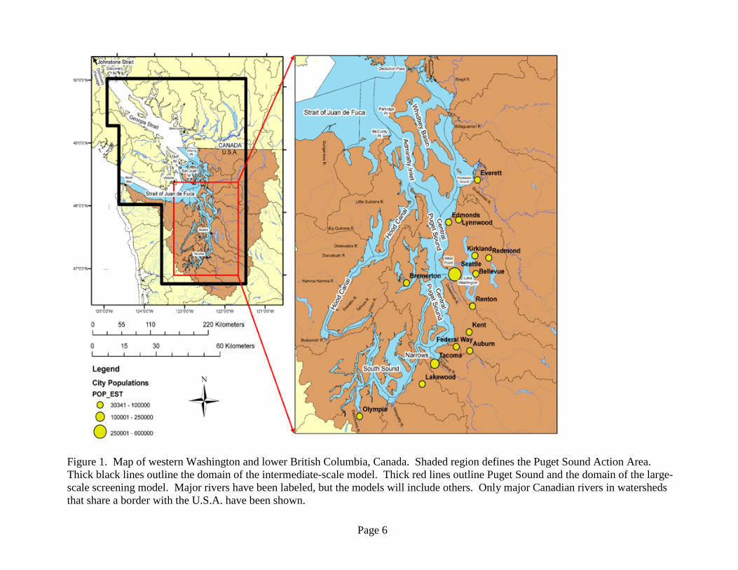
Figure 1. Map of western Washington and lower British Columbia, Canada. Shaded region defines the Puget Sound Action Area. Thick black lines outline the domain of the intermediate-scale model. Thick red lines outline Puget Sound and the domain of the large-scale screening model. Major rivers have been labeled, but the models will include others. Only major Canadian rivers in watersheds that share a border with the U.S.A. have been shown.

Page 7

These characteristics of Central Puget Sound facilitated the diversion of sewage from Lake Washington to West Point (Puget Sound) in the late 1950s (Edmondson, 1991). While nutrient loading to Lake Washington caused excessive algal growth in the lake, the same loading at West Point did not appear to enhance algal growth in marine (salt) waters. Much of the current understanding of Puget Sound phytoplankton dynamics has been based on modeling and measurements of ambient productivity and nutrients at West Point (Winter et al., 1975). In contrast, a more recent study by Newton and Van Voorhis (2002) observed substantial increases in algal primary production when water samples from Central Puget Sound and Possession Sound were artificially enriched with nutrients. Nutrient-enhanced production was observed at all stations, but the degree of enhancement varied both spatially and temporally. This suggests that the system is more complex and that there are likely to be a diversity of responses to nutrient addition. These responses are expected to manifest differently at different times and locations within greater Puget Sound. Mackas and Harrison (1997) evaluated the issue of eutrophication in the Strait of Juan de Fuca, Georgia Strait, and Puget Sound. They judged potential impacts from eutrophication of Central Puget Sound to be relatively low. However, they reported that the most sensitive sub-regions are likely to be small tributary inlets and fjords that have low flushing rates and that adjoin urbanized shorelines. They speculated that the “early warning signs of eutrophication” were already becoming evident in these areas. At present, most of these areas lie along the south and west margins of Puget Sound. Bricker et al. (1999) later reported the overall level of expression of eutrophic conditions to be moderate in Central Puget Sound and Whidbey Basin and high in Hood Canal and South Puget Sound. They predicted conditions to worsen, especially in Hood Canal and South Puget Sound, due to increasing population pressures. In response to the increasing threat of nutrient-stimulated eutrophication in Puget Sound, Ecology has both initiated and been actively involved with the continuation of focused water quality studies in these areas (Roberts et al., 2009a; Albertson et al., 2007; Roberts et al., 2005b; Albertson et al., 2002).

Project Description This project capitalizes on what has been learned in these prior studies and seeks to expand this foundation to develop a unified water quality model applicable to the entire Puget Sound estuary system. As part of mandates under the Federal Clean Water Act to manage pollutant loading to meet water quality standards, EPA, Pacific Northwest National Laboratory (PNNL), and Ecology have jointly initiated this water quality model development project to address the following nutrient management questions.

• Are human sources of nutrients in and around Puget Sound significantly impacting water quality?

• How much do we need to reduce human sources of nutrients to protect water quality in Puget Sound?

Page 8

PNNL will develop the hydrodynamic and water quality models for use by the agencies. These models will evaluate the effect of human sources of nutrients on dissolved oxygen across Puget Sound and define potential Puget Sound-wide nutrient management strategies and decisions. The model development will occur in PNNL’s Marine Sciences Laboratory, through an intergovernmental agreement between PNNL and Ecology. This document describes the development of this intermediate-scale model of Puget Sound. A complementary Quality Assurance Project Plan has been created which details development of the large-scale screening model (Sackmann, 2009).

Project Goals and Objectives Mechanistic models provide the quantitative framework necessary to (1) integrate the diverse physical, chemical, and biological information that constitute complex environmental systems and (2) provide a vehicle for an enhanced understanding of how the environment works as a unit (Chapra, 1997). For example, the following cannot be determined without a quantitative approach:

• Complexities such as the impact of the temporal and spatial distribution of nutrient additions, of when freshwater inputs occur and how that alters circulation patterns.

• Co-limitation of production by nutrient and sunlight.

In this study the water quality models to be developed will identify and assess factors and processes that influence water quality in Puget Sound on a significant scale. The overall goal of this project by Ecology is to work collaboratively with EPA, PNNL, and a Project Advisory Committee (PAC) to conduct DO modeling in Puget Sound in a manner that complements and supports concurrent management initiatives. This project consists of the following components: 1. Two multi-purpose hydrodynamic models for the entire Puget Sound, one at a large scale

(based on Babson et al., 2006) and one at an intermediate scale. These models can also serve as community tools for other purposes.

2. The large-scale model (also called “box model”) will be used to produce a screening-level evaluation of nutrient effects on DO, Puget-Sound-wide. The results of this effort will inform the intermediate-scale model.

3. The intermediate-scale model (also called the “intermediate-grid model”) will be used to evaluate the effect of human-caused nutrient enrichment on DO across Puget Sound. This model will help determine potential Puget-Sound-wide management strategies and decisions and would support site-specific detailed work that may be completed beyond this project.

4. A Quality Assurance (QA) Project Plan for a detailed site-specific analysis for one Puget Sound basin (e.g., Whidbey basin) to determine the nutrient-loading reductions needed to meet water quality standards.

Page 9

The scope and focus of this QA Project Plan is limited to the development of the intermediate-scale model (i.e., items 1 and 3 above) only. The development strategy for the large-scale model is described in a separate QA Project Plan (Sackmann, 2009). Objectives specific to this project are as follows:

• Develop an intermediate-scale water quality model, calibrated to conditions observed in Puget Sound during 2006.

• Estimate effects of nutrient loading on DO and apply the model to various nutrient-loading scenarios.

• Evaluate sensitivity of the model to various input parameters and boundary conditions.

Page 10

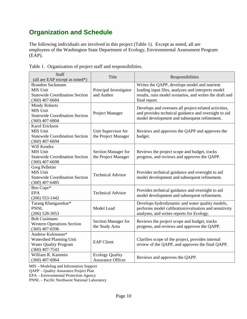
Organization and Schedule The following individuals are involved in this project (Table 1). Except as noted, all are employees of the Washington State Department of Ecology, Environmental Assessment Program (EAP). Table 1. Organization of project staff and responsibilities.

Staff (all are EAP except as noted*) Title Responsibilities

Brandon Sackmann MIS Unit Statewide Coordination Section (360) 407-6684

Principal Investigator and Author

Writes the QAPP, develops model and nutrient loading input files, analyzes and interprets model results, runs model scenarios, and writes the draft and final report.

Mindy Roberts MIS Unit Statewide Coordination Section (360) 407-6804

Project Manager Develops and oversees all project-related activities, and provides technical guidance and oversight to aid model development and subsequent refinement.

Karol Erickson MIS Unit Statewide Coordination Section (360) 407-6694

Unit Supervisor for the Project Manager

Reviews and approves the QAPP and approves the budget.

Will Kendra MIS Unit Statewide Coordination Section (360) 407-6698

Section Manager for the Project Manager

Reviews the project scope and budget, tracks progress, and reviews and approves the QAPP.

Greg Pelletier MIS Unit Statewide Coordination Section (360) 407-6485

Technical Advisor Provides technical guidance and oversight to aid model development and subsequent refinement.

Ben Cope* EPA (206) 553-1442

Technical Advisor Provides technical guidance and oversight to aid model development and subsequent refinement.

Tarang Khangaonkar* PNNL (206) 528-3053

Model Lead Develops hydrodynamic and water quality models, performs model calibration/evaluation and sensitivity analyses, and writes reports for Ecology.

Bob Cusimano Western Operations Section (360) 407-6596

Section Manager for the Study Area

Reviews the project scope and budget, tracks progress, and reviews and approves the QAPP.

Andrew Kolosseus* Watershed Planning Unit Water Quality Program (360) 407-7543

EAP Client Clarifies scope of the project, provides internal review of the QAPP, and approves the final QAPP.

William R. Kammin (360) 407-6964

Ecology Quality Assurance Officer Reviews and approves the QAPP.

MIS – Modeling and Information Support QAPP – Quality Assurance Project Plan EPA – Environmental Protection Agency PNNL – Pacific Northwest National Laboratory

Page 11

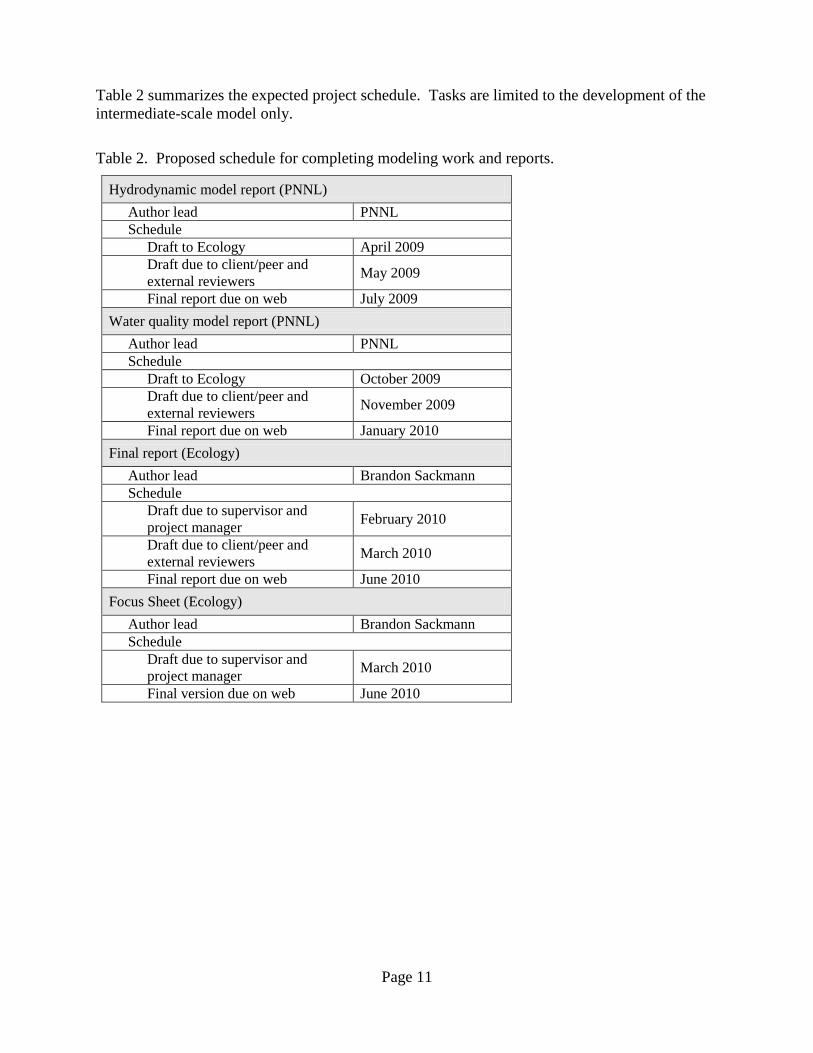
Table 2 summarizes the expected project schedule. Tasks are limited to the development of the intermediate-scale model only.

Table 2. Proposed schedule for completing modeling work and reports.

Hydrodynamic model report (PNNL) Author lead PNNL Schedule

Draft to Ecology April 2009 Draft due to client/peer and external reviewers May 2009

Final report due on web July 2009 Water quality model report (PNNL)

Author lead PNNL Schedule

Draft to Ecology October 2009 Draft due to client/peer and external reviewers November 2009

Final report due on web January 2010 Final report (Ecology)

Author lead Brandon Sackmann Schedule

Draft due to supervisor and project manager February 2010

Draft due to client/peer and external reviewers March 2010

Final report due on web June 2010 Focus Sheet (Ecology)

Author lead Brandon Sackmann Schedule

Draft due to supervisor and project manager March 2010

Final version due on web June 2010

Page 12

Capabilities for a Dissolved Oxygen Model of Puget Sound

The success of marine circulation and water quality model development can be affected by the choice of the software tool and modeling framework. Ecology assembled a Model Technical Advisory Committee (MTAC) to seek input on modeling approaches, given the project goals and resources. The MTAC is comprised of modeling professionals and is separate from the PAC, although some membership overlaps. The MTAC evaluated the key processes needed in the model, extent of model domain, level of detail, model framework comparison (pros/cons), and model applicability to other Puget Sound projects. Ecology convened a MTAC workshop on November 4, 2008 which was attended by modeling experts and the project team. The information and feedback received has been summarized and is attached as Appendix A. While Ecology is responsible for the final model selection in consultation with the project team and MTAC, Ecology has requested that PNNL also provide input on model selection separately, in the capacity of a team member responsible for the model development and implementation. Recommendations are based on Puget Sound hydrodynamic features, experience with various models and tools available, and understanding of project goals. PNNL’s assessment of the model performance requirements is provided below. Models and software tools are limited to those available in the public domain. Commercial models such as Delft-3D, WQMAP, MIKE, and other similar tools were not included in this assessment. If the results are used for regulatory purposes, all model information must be available to interested parties. Proprietary or commercial models do not satisfy this need.

Hydrodynamics Puget Sound is a large estuarine system bounded by 2,597 miles of complex shorelines and consists of several subbasins and many large estuaries with distinct properties of their own. It is the largest such body of water in the contiguous 48 states. Pacific Ocean water enters the Puget Sound estuary system and the Georgia Strait through the Strait of Juan de Fuca (SJF) entrance at Neah Bay. The SJF is also the outlet for most of the freshwater discharged from the Puget Sound and from the Fraser River in British Columbia. Admiralty Inlet links the three major branches of Puget Sound together and serves as the primary outlet to the SJF and ultimately the Pacific Ocean. The three main branches of Puget Sound are:

1. The deep Main Basin and the shallower South Sound (separated from the Main Basin by a sill and constriction at the Narrows).

2. Hood Canal.

3. Whidbey Basin. The only other outlet to SJF is the extremely narrow Deception Pass located at the northern end of Whidbey basin (Figure 1).

Page 13

The large freshwater discharge from the Fraser River affects stratification and currents in the adjacent waters of the SJF and Georgia Strait including waters around San Juan Islands and the Cherry Point coastline near the U.S./Canada border. There is considerable interest in the circulation and transport in the entire region spanning the U.S. and Canadian waters for the assessment of fish migration patterns and pathways. Although not the primary focus of this study, there is also an interest in understanding the effect of nutrient loads entering Puget Sound from Canadian waters. Therefore, there is a need to ensure that the study domain extends well north into Canadian waters to Johnstone Strait near the entrance to Discovery Passage. The circulation in Puget Sound shows distinct fjordal three-dimensional (3D) characteristics with mean outflow in the surface layers and inflow in the lower layers. Near the mouths of the individual estuaries there is stratification due to freshwater discharge and complex circulation patterns induced by cross flow as the river plumes encounter Puget Sound tidal influences. The model selected must therefore be capable of simulating (1) 3D baroclinic (density-induced) circulation affected by freshwater inflows over shallow mudflats and (2) sharp changes in bathymetry to deep fjordal depths of Puget Sound. The currents are also affected by local winds. Several models available in the market are capable of addressing the above characteristics. These are being used successfully on various studies in progress in Puget Sound and are possible candidates for this study: • EFDC (Roberts et al., 2005a; Khangaonkar and Yang, 2004; King County, 1999). • CH3D (Johnston et al., 2007). • POM (Kawase, 1998). • SUNTANS (Wang et al., 2008). • FVCOM (Finite Volume Community Ocean Model; Yang and Khangaonkar, 2008). • RMA10 (Breithaupt et al., 1999). • UnTRIM (Joshberger and Cheng, 2005). • ROMS (Bahng et al., 2007).

Water Quality The focus of this project is on simulating the response of dissolved oxygen concentrations to nutrient loading. Eutrophication and algal kinetics are of major interest because they are the links between nutrients and dissolved oxygen. Parts of Puget Sound such as the Hood Canal and the nearshore estuarine and riverine reaches have shown evidence of hypoxia. A full listing of various processes of interest and variables which need to be simulated is discussed in Puget Sound Dissolved Oxygen Modeling, Model Technical Advisory Committee, Model Selection Workshop Summary (Appendix A). The selected model must have the ability to simulate full eutrophication kinetics. This includes the ability to incorporate point sources, as well as address multiple algal groups, nutrient cycling, and sediment oxygen demand (SOD) and biochemical oxygen demand (BOD) processes. Nutrient loads will be specified as input variables for all important sources. These loads will be estimated by Ecology using data from the National Pollutant Discharge Elimination System

Page 14

(NPDES) database, the river and stream monitoring network data, and the South Puget Sound Dissolved Oxygen Study (Roberts et al., 2009b). Most of the models described above, such as EFDC, CH3D, ROMS, FVCOM, and RMA10, have sophisticated water quality modules which may be applied for this study. In models other than RMA10, the water quality modules are embedded within the codes, coupled to hydrodynamics, and could impose a considerable computational burden. CH3D and EFDC models have been used in decoupled mode with stand-alone water quality simulation programs such as WASP (Wool et al., 2006) and CE-QUAL-ICM (Cerco and Cole, 1995).

Ability to Incorporate Nearshore Processes at High Resolution This phase of the project seeks to establish a model at an intermediate-scale improving in resolution over the large-scale model (also called “box model”) of Puget Sound (Babson et al., 2006). The intermediate-scale model will be set up at a resolution sufficient for addressing the large-scale questions on the assimilative capacity of Puget Sound. However, the model could be used subsequently to address localized high-resolution processes including the effects of point source discharges and water quality impairment in the nearshore regions associated with sediment and bacteria contamination. The ability of the model to improve resolution as required through the use of nested grid techniques or the use of unstructured grids is considered essential for future applications in Puget Sound such as Total Maximum Daily Load (TMDL) calculations or sediment impact zone (SIZ) assessment for remedial investigations. Therefore, model capabilities to address additional parameters beyond dissolved oxygen are considered but are not essential.

Summary Appendices B and C show a listing of available hydrodynamic and water quality modeling tools, their capabilities, and ranking based on comments provided by the MTAC. As seen in Appendix B, hydrodynamic models are largely divided into structured grid models (POM, EFDC, ROMS, CH3D and GEMSS) and unstructured grid models (FVCOM, UnTRIM, ADCIRC, and SELFE). Most of them use high-order transport schemes, wetting/drying option, and a sigma-grid system. These models are well known, well tested, and have been applied on many projects. Many of these models have active user groups and provide well-organized technical documentation.

Page 15

Recommendation for Model Selection and Model Approach

If the selection were based on immediate project goals and model skill and capabilities alone, a number of available models discussed above could provide the required performance. However, our interest in developing a tool which could be used over the long term by a broader community of scientists requires consideration of the following additional points. • Applicability to Ecosystem Model Development Efforts: A number of agency groups

including NOAA Fisheries and King County are engaged in developing an ecosystem / food web model of Puget Sound. A Puget Sound Dissolved Oxygen / Water Quality Model could be used as a source of information on temperature, salinity, nutrient concentrations, dissolved oxygen, and other conventional water quality variables which are desired inputs to ecosystem modeling efforts. In addition, the ability of this model to also provide information about metals, organics, and sediment contamination levels will be a major plus with respect to supporting sediment remediation.

• Ability to Conduct Long-duration Model Runs: The effects of climate change and sea

level rise are issues of considerable interest. The ability of the model to be used in the future to conduct simulations over 10-year to 100-year timeframes is an important consideration.

• Wetting and Drying, Mudflats, and Nearshore Circulation: Much of the effort in

connection with restoration of Puget Sound is focused on the nearshore. The question often posed is “Can we achieve beneficial restoration outcomes at the fine local scale, as well as at a large estuary-wide scale?” Capabilities of the model for simulating the important nearshore processes are essential both for immediate dissolved oxygen simulation needs and for potential long-term modeling needs of this region. Examples of these processes are circulation in complex multiple tidal channels, wetting and drying of tide flats, and water quality and sediment transport.

Based on model performance requirements discussed in the previous section and additional points listed above, model recommendations are as follows: 1. Unstructured Grid Framework: The model framework must incorporate an unstructured

grid framework to be able to address nearshore processes adequately while simultaneously assessing the circulation and water quality of the entire Puget Sound. The ability to modify the grid efficiently as new information and data become available is considered essential for developing a model of a complex water body such as Puget Sound.

2. Comprehensive Water Quality Model Decoupled from Hydrodynamics: It is unlikely

that a complete water quality model will be developed through a single effort. It is likely that more features and processes will be added through subsequent project applications. Multiple users may wish to apply the modeling framework to look at other parameters of interest (e.g., bacteria, toxics, submerged aquatic vegetation). It is therefore important to select a water quality model framework with the ability to address a wide range of processes. From a

Page 16

computational efficiency standpoint, access to a water quality module which is independent of the hydrodynamic tool is highly recommended.

PNNL reviewed a number of unstructured grid models and contacted the authors to discuss the strengths and weaknesses of their tools. These included the leading 3D unstructured grid models:

• RMA10 (King, 1998). • ADCIRC (Luettich et al., 1992). • ELCIRC (Zhang et al., 2004). • SELFE (Zhang and Baptista, 2008). • UnTRIM (Casulli and Walters, 2000). • FVCOM (Chen et al., 2003). The SUNTANS model discussed in the previous section is considered under development with respect to its ability to handle shallow mudflats and wetting and drying, and does not include associated water quality. The ADCIRC model is popular for storm surge modeling in barotropic mode, but the baroclinic version of the model is not yet available. The UnTrim model is not generally available in public domain. The ELCIRC model of the Columbia River and Washington Coast previously developed by the Oregon Graduate Institute had a strict limiting requirement of orthogonal grid cells, and has now been replaced by SELFE. The water quality module of SELFE is still under development. PNNL is closely following the development of the SELFE and SUNTANS unstructured grid hydrodynamic modeling tools. Based on testing and application on numerous projects, Ecology recommends the FVCOM model for this project. FVCOM simulates water surface elevation, velocity, temperature, salinity, and sediment and water quality constituents in an integral form by computing fluxes between non-overlapping, horizontal, triangular control volumes. This finite-volume approach combines the advantages of finite-element methods for fitting complex boundaries and finite-difference methods for simple discrete structures and computation efficiency. A sigma-stretched coordinate is used in the vertical plane to better represent the irregular bottom topography. Unstructured triangular cells are used in the horizontal plan. Key features of FVCOM on which the selection is based are detailed in Appendices B and C but are summarized as follows.

• Unstructured grid modeling framework. • Ability to simulate baroclinic circulation. • Finite volume technique with good mass conservation properties. • Wetting and drying simulation. • Parallelized code (hydrodynamics) for cluster computing. • Availability of water quality, sediment transport, and particle tracking. • Public domain and well-tested code on multiple projects with an active research group. Although a water quality component (NPZD) is available through FVCOM, Ecology recommends selection and application of a water quality tool which may be applied independent of the hydrodynamic model in a decoupled mode.

Page 17

WASP and CE-QUAL-ICM are two water quality models which have been extensively used in the U.S. The coupled water quality modules in many of the tools discussed previously are based on these two models. The models are applicable over an unstructured hydrodynamic model grid. They incorporate a comprehensive suite of water quality processes including conventional eutrophication, and toxics fate and transport kinetics. The CE-QUAL-ICM model provides added capabilities with respect to sediment diagenesis and the ability to incorporate submerged aquatic vegetation. Based on the above considerations, Ecology’s selections for the Puget Sound Dissolved Oxygen model are as follows: • Hydrodynamics – An intermediate-scale hydrodynamic model of Puget Sound using the

FVCOM model developed by the University of Massachusetts.

• Water quality – A decoupled application of the U.S. Army Corps of Engineers CE-QUAL-ICM model to be operated using the FVCOM model grid and pre-computed hydrodynamic solution.

Ecology will work with PNNL, EPA, and the MTAC to develop an approach for model setup. This will include grid resolution (vertical and horizontal), selection of input and output data, model calibration/evaluation, and application.

Page 18

Hydrodynamic Model Setup

Development of the intermediate-scale hydrodynamic model will consist of three steps:

1. Model grid development. 2. Model setup involving specification of boundary conditions for the selected period. 3. Calibration and sensitivity analysis.

1. Grid Development The grid development activity and preparation of model input files are part of the model setup and are specific to the modeling system selected. PNNL has previously developed a high-resolution model of the Puget Sound. In doing so, a detailed bathymetry file for Puget Sound using a combination of digital elevation maps, LiDAR data, and hydrographic surveys has been prepared. Using this data set, the Puget Sound domain will be re-gridded extending from the mouth of the Strait of Juan de Fuca to South Puget Sound. The northern boundary will be set at the entrance to Johnstone Straits past the Fraser River north of Vancouver B.C. (Figure 1). The resolution selected will be considerably finer than the large-scale model, ensuring reasonable representation of the various subbasins within Puget Sound. However, the grid will be coarse relative to the PNNL Puget Sound model, which has a resolution as fine as 30 feet in certain subbasins.

2. Boundary Conditions and Meteorological Forcing We expect that the model will be set up with sufficient layers (10 to 30) in the vertical to address the highly stratified nature of residual circulation in Puget Sound. In Puget Sound, a synoptic data set for currents and tides covering the entire domain is not available. Therefore the hydrodynamic model setup will need to be tested against the multiple periods of 9/96, 9/04, 10/06, and 9/07 during which data were collected. These periods also match the calibration periods for the fine-resolution PNNL hydrodynamic model previously completed. There are 17 major rivers that discharge into Puget Sound and its adjacent waters. Most of these rivers have real time USGS streamflow gages. Contributions from the rest of the land surface will also be included for completeness but not necessarily representing each stream mouth. The model will be set up with flows from these rivers included as boundary source terms. However, the estuarine circulation, the movement of salt wedge, and the upstream tidal intrusion generated by these river inflows are beyond the scope of the intermediate-scale model. Tidal elevations at the open boundaries will be specified using the XTIDE predictions based on NOAA National Oceanic Service algorithms. At the water surface, wind stress will be specified. Wind will be included for completeness with wind stress being initially applied uniformly across the entire model domain for simplicity. Meteorological forcing terms, including wind and heat flux or air temperature and solar radiation, will be specified using either (1) direct measurements

Page 19

or (2) MM5 or WRF meteorological model simulations if the latter are sufficient for this model application.

3. Calibration Strategy Model calibration, described below, will be conducted by comparing the predicted tides, currents, and salinity and temperature profiles to observed data. The process of calibration will consist of steps such as refining the model grid as required, adjusting bottom roughness and friction, and varying tidal phase along open boundaries. Once the model calibration is completed, sensitivity analysis will be performed testing the stability and reliability of the model to a wide range of inputs. Tidal residual calculations will also be performed as part of the sensitivity analysis.

Page 20

Water Quality Model Setup

The objective of this intermediate-scale water quality and nutrient model is to develop a large-scale understanding of the nutrient assimilation capacity of Puget Sound. The selected water quality model will simulate conventional water quality constituents such as nitrogen, phosphorus, dissolved oxygen, BOD, SOD, phytoplankton, and temperature. The focus of this modeling effort is on the response of the above listed variables to nutrient loads, which is conventionally known as the eutrophication cycle. PNNL will set up the selected model over the same domain and grid developed for the hydrodynamic model. The initial preference is to develop the water quality model in a de-coupled configuration so that it may be applied repeatedly using previously computed hydrodynamic solutions. Although this is not a requirement, it does provide benefits in terms of model runtimes.

Nutrient Loads and Boundary Conditions Nutrient loads will be specified as input variables for all important sources. These loads will be estimated by Ecology using data from the NPDES database and river and stream monitoring network data. Data for the marine boundary conditions will be established using a combination of (1) water quality data collected by Fisheries and Oceans Canada’s Southern BC Coastal Waters Monitoring project and (2) historical observations from NOAA’s World Ocean Database and various satellite-derived data products, as appropriate.

Algal Dynamics The effect of zooplankton grazing on phytoplankton will be parameterized as a first-order loss process. We anticipate that two or three algal groups will be used to represent phytoplankton dynamics in Puget Sound. This decision is based, in part, on a desire to minimize the use of time-varying kinetics while retaining some flexibility with respect to the parameters used to describe various algal processes. Our choice was further reinforced by a strong recommendation from Robert Ambrose1

1 Environmental Engineer with EPA’s Ecosystems Research Division and co-developer of the Water Quality Analysis Simulation Program (WASP).

that more than one algal group be used any attempt to model a complicated biological system such as Puget Sound. First-order grazing appropriately represents seasonal variations, and bloom-scale responses are not the target.

Page 21

Loading Estimation

Nutrient Sources Excess nitrogen can come from a variety of sources. The term nonpoint source is used to describe diffuse sources that do not come through a pipe (such as rainfall runoff from agricultural fields and residential yards) and groundwater (including contributions from septic systems). Most of the nonpoint nitrogen loading from the watersheds surrounding Puget Sound enters via rivers and streams. The term point source generally refers to sources that are regulated under the federal Clean Water Act through the NPDES. NPDES permits are issued to municipal and industrial wastewater treatment plants (WWTPs) and stormwater systems, constructions sites, boatyards, salmon net pens, and other facilities. With respect to point sources, municipal WWTPs that discharge directly to Puget Sound are thought to represent the largest anthropogenic source of direct nitrogen loading from the watershed to the Sound. A few industrial facilities discharge directly to Puget Sound. These will be included where discharge information is available or can be estimated. Point source loads will be estimated using data from the NPDES database and the South Puget Sound Dissolved Oxygen Study (Roberts et al., 2009b). In some cases, smaller wastewater discharges may be combined. We will provide each treatment facility with an opportunity to review, comment on, and possibly update data being used to describe their site. In addition to providing them with an inventory of the available water quality data, we will include our estimate for the location of each outfall, the number of grid cells that will be required to describe it in the model domain, and how we anticipate incorporating the point source into the model (e.g., discharge of effluent at depth). While all rivers are generally considered nonpoint sources, some have upstream WWTPs that discharge to freshwater. For this project, upstream WWTPs will not be separated out of the river and stream inputs. In addition, rivers and streams receive discharges from other permitted areas, such as municipal stormwater, which are considered point sources. Again, for this project, permitted sources will not be separated out of the river and stream inputs.

Data Requirements A major activity as part of the model setup will be developing nutrient-loading input files for all WWTPs and major rivers. Ecology’s goal is to develop these files as a separate stand-alone product to facilitate their use by other projects and agencies. This project will require the following information for specifying nutrient loads from all sources including effluent dischargers and major river loads:

• Flow rates and temperature data. • Organic phosphorus (particulate and dissolved).

Page 22

• Dissolved phosphorus (soluble reactive phosphorus). • Organic nitrogen (particulate and dissolved). • Ammonia nitrogen. • Nitrate + Nitrite nitrogen. • Dissolved oxygen (DO). • pH. • Total organic carbon (TOC). • Dissolved organic carbon (DOC). • Carbonaceous biochemical oxygen demand (CBOD to be estimated from DOC or DOC to be

estimated from CBOD, as needed). When available, measured effluent quality for a particular point source will be used to estimate its constituent loadings. If such data are not available for a particular source, it will be necessary to estimate effluent quality based on measurements from similar facilities. Organic nitrogen may be estimated as the difference between (1) total Kjeldahl nitrogen and ammonia nitrogen for WWTPs and (2) total nitrogen and the sum of ammonium, nitrate, and nitrite for rivers. Organic phosphorus may be estimated as the difference between total phosphorus and orthophosphate phosphorus.

Estimation Methods As mentioned earlier under ‘Hydrodynamics Model Setup’, there are 17 major rivers that discharge into Puget Sound and its adjacent waters, most of which have real time USGS streamflow gages. Calculation of river loads requires both constituent-concentration and streamflow data. As part of the USGS National Water Quality Assessment, Embrey and Inkpen (1998) estimated nutrient loads to Puget Sound from several major rivers based on existing nutrient concentrations and discharge data for the period 1980-1993. Using an analogous approach, time-resolved stream loads will be estimated for 2006 using (1) constituent-concentration data compiled from databases maintained by agencies operating water-quality monitoring stations in the Puget Sound Basin and (2) streamflow estimates made at the time of water-quality sample collection (Appendix D). The intermediate-scale model will be set up with flows from rivers included as boundary source terms. The model will require daily time series of flows, temperature, dissolved oxygen, pH, and nutrient loads from discrete watershed inflow points to simulate seasonal and subseasonal variations in Puget Sound water quality. The total ungaged discharge to Puget Sound may be as high as 10% of the total gaged inflow but with potentially higher nutrient concentrations due to agricultural and urban runoff. Flows from ungaged rivers will be estimated by first choosing a representative gaged reference river based on its similarity to an ungaged area and then multiplying the reference flow by the ratio of the ungaged to gaged areas (Lincoln, 1977). In cases where rivers are gaged well upstream from the river mouth, the drainage area downstream of the station is used as the ungaged area in the calculation, and the estimated flow is added to the gaged flow to obtain total discharge for that river.

Page 23

Following Mohamedali (2009) and Roberts and Pelletier (2001), daily time series of various parameters and nutrient concentrations will be estimated using multiple linear regressions (Cohen et al., 1992). This analysis is based on the premise that parameter concentrations can be predicted based on flow and time of year. The multiple linear regression equation to be used in this analysis is given by: log(c) = b0 + b1log(Q/A) + b2[log(Q/A)]2 + b3sin(2πfy) + b4cos(2πfy) + b5sin(4πfy) + b6cos(4πfy) (1) where: c is the observed parameter concentration (mg/L) or in the case of temperature or pH it is in oC and pH units (respectively). Q is discharge (m3/s). A is the area drained by the monitored location (km2). fy is the year fraction (dimensionless, varies from 0 to 1). bi is the best-fit regression coefficients. All six variables in the above equation are known values (from available concentration data, streamflow data, watershed area, and time of year) except for the coefficients (bi). The multiple linear regression model attempts to solve equation (1) and determine the optimum combination of bi coefficients that will yield the best fit between predicted and observed concentrations of a specific parameter. Once these coefficients are determined, the above equation can be used to predict parameter concentrations continuously over any time period (for example, at a daily interval). Daily concentrations will be multiplied with daily streamflow data to predict daily loads for time periods of interest. In previous applications of this regression model methodology, certain water quality parameters were better characterized by the regression model than others, particularly those highly influenced by flow and seasonality. Though the statistical results from some parameters suggested a poor fit for concentration, predicted daily loads often compared well with observed loads for most parameters across a wide variety of streams. There is also evidence that groundwater may contribute significant amounts of freshwater to some basins (e.g., Hood Canal) and should be evaluated as a potential source of distributed nutrients. One proposed application of the model will be to test the relative sensitivity of this source, using published and/or order-of-magnitude groundwater flow estimates, to the overall nutrient and dissolved oxygen balance of Puget Sound (Simonds et al., 2008).

Canadian Sources Loads from Canadian sources will be calculated to determine Puget Sound’s sensitivity to nutrients coming into the system through its northern boundary. Daily loads will be estimated using methods analogous to those used in Puget Sound. However, initially loads will only be estimated for major rivers and WWTPs. These are likely to include (but will not be limited to) loads from the Fraser River, Victoria-area WWTPs, and Vancouver-area WWTPs. Should the water quality model results in Puget Sound prove sensitive to these Canadian sources, then additional analyses will be performed to more accurately quantify and include the effects from more of the smaller rivers/streams and WWTPs within the model domain.

Page 24

Available Data Sources

Acceptance Criteria No data collection is planned for this project, and specific quality objectives are not being specified for existing data or for modeling results. However, data from existing repositories will be used for model calibration and evaluation purposes, and the following acceptance criteria will be applied: • Data Reasonableness. Data quality of existing data will be evaluated where available. Best

professional judgment will be used to identify erroneous or outlier data, and these observations will be removed from the data set.

• Data Representativeness. Data will be used that are reasonably complete and representative

of the location or time period under consideration. Incomplete data sets will be used if they are considered representative of conditions during the period of interest. Data from outside the period of interest will be used only if no other data are available. In this case, best professional judgment will be used to determine the utility of the available data.

• Data Comparability. Long-term water quality monitoring programs often collect, handle,

preserve, and analyze samples using methodologies that evolve over time. Best professional judgment will be used to determine whether/if data sets can be compared. The final project report will detail any caveats or assumptions that were made when using data collected with differing sampling or analysis techniques.

Data Set Descriptions This list identifies those repositories that contain relevant data. However, additional sources of information may be considered as needed and/or as new sources are identified. Below is a description of each repository identified in Appendix D along with a URL describing each program in more detail. In most cases, data are available in electronic format. Washington State Department of Ecology (Ecology) Marine Waters Monitoring Data Ecology has monitored water quality at approximately 40 stations within Puget Sound on a monthly basis since 1975. Some stations are monitored every year while some are monitored on a rotating schedule.

www.ecy.wa.gov/programs/eap/mar_wat/mwm_intr.html

Page 25

Ecology South Puget Sound Field Studies Ecology has been conducting a water quality study focused on low dissolved oxygen levels in South Puget Sound. Field surveys occurred from 1994 to 2007. Data include both river and wastewater treatment plant (WWTP) effluent water quality.

www.ecy.wa.gov/puget_sound/dissolved_oxygen_study.html Ecology Central Basin/Possession Sound Primary Production Study From October 1998 through October 2001, Ecology conducted a study to assess whether primary production in Central Puget Sound and Possession Sound would be affected by the addition of nutrients (Newton and Van Voorhis, 2002). Data collected during this study will provide rate estimates for algal production as a function of light, season, and other controlling factors. www.ecy.wa.gov/biblio/0203059.html Ecology Puget Sound Mooring Data Since 2005, Ecology has maintained three moorings in Puget Sound to provide continuous data for investigation of status and trends of marine water quality. The moorings are located at piers and docks in Budd Inlet, Squaxin Passage, and Clam Bay. They provide 15-minute values for temperature, conductivity (used to calculate salinity), dissolved oxygen, and chlorophyll a fluorescence.

www.ecy.wa.gov/programs/eap/mar_wat/moorings.html Ecology Freshwater Ambient Monitoring Data Ecology maintains a freshwater ambient monitoring network that includes numerous sites on rivers and streams within the greater Puget Sound area. www.ecy.wa.gov/programs/eap/fw_riv/rv_main.html Hood Canal Dissolved Oxygen Program (HCDOP) HCDOP is a partnership of 28 organizations that conducts monitoring and analysis to determine sources of and potential corrective actions for low dissolved oxygen in Hood Canal and its effects on marine life. HCDOP monitors marine water quality as well as water quality in rivers, streams, and groundwater sources that discharge into Hood Canal. Monitoring of present-day water properties in the canal is done using a combination of target field efforts, citizen volunteers, and by moorings with near-real-time data transmission capabilities. (See description of ‘APL ORCA Mooring Data’ below.) www.hoodcanal.washington.edu/

Page 26

UW Applied Physics Laboratory (APL) ORCA Mooring Data Oceanic Remote Chemical Analyzers (ORCA) are autonomous moored profiling systems that provide real-time data streams of water and atmospheric conditions. They consist of a profiling underwater sensor package and a surface-mounted weather station. Currently there are four ORCA mooring systems deployed, all in Hood Canal. Past deployments of the ORCA system have been in South Puget Sound (Carr Inlet) and Central Puget Sound (near Point Wells). www.orca.ocean.washington.edu/ UW PRISM Field Studies In partnership with Ecology, the University of Washington PRISM (Puget Sound Regional Synthesis Model) program conducted approximately twice-annual monitoring cruises encompassing approximately 40 stations located throughout Puget Sound. These started in June 1998 and continued through July 2004.

www.prism.washington.edu/

King County DNR Puget Sound Marine Monitoring Data King County’s Marine and Sediment Assessment Group supports a comprehensive, long-term marine monitoring program that assesses water quality in Central Puget Sound. Their program consists of offshore water quality, beach water quality, intertidal sediment, algae, and clam monitoring.

www.green.kingcounty.gov/marine/Index.htm King County DNR Stream and River Monitoring Data Many streams and rivers in the King County service area are assessed as part of the routine monitoring efforts by the King County Major Lake and Stream Monitoring Program. Monthly baseflow water quality samples have been collected at many of these sites since 1976. Data are analyzed to characterize the general water quality of the stream, determine if applicable state and federal water quality criteria are met, and to identify long-term water quality trends.

www.green.kingcounty.gov/WLR/Waterres/StreamsData/ Skagit County Water Quality Monitoring Program Data The Skagit County Monitoring Program was designed to determine water quality conditions and trends in agricultural-area streams in Skagit County. The bi-weekly sampling at 40 sites began in October 2003. It is being conducted by Skagit County Public Works Surface Water Management through September 2009.

www.skagitcounty.net/scmp

Page 27

USGS Freshwater River/Stream Data The United States Geological Survey maintains a network of streamflow gaging stations, including sites in the study area. www.waterdata.usgs.gov/wa/nwis/rt Sinclair/Dyes Inlet Flow Data The U.S. Navy’s Puget Sound Naval Shipyard, in partnership with a variety of federal, state, and local governments, tribes, and community groups, developed and maintained a flow network for streams and creeks tributary to Sinclair and Dyes Inlets from 2001 to 2005 (May et al., 2005).

www.ecy.wa.gov/programs/wq/tmdl/sinclair dyes_inlets/sinclair_cd/DATA/Data_Directory.html

NPDES Data Wastewater treatment plant monthly data reported under NPDES permits are available through the Water Quality Permit Life Cycle System (WPLCS).

www.ecy.wa.gov/programs/wq/permits/wplcs/index.html

Canadian Data Set Descriptions This list identifies those repositories that contain relevant data for Canadian waters. However, additional sources of information may be considered as needed and/or as new sources are identified. A URL has been provided that describes each program in more detail. In most cases, data are available in electronic format. Water Survey of Canada (WSC) National Water Quantity Survey Program Data WSC is the national agency responsible for the collection, interpretation, and dissemination of standardized water resource data and information in Canada. This includes data on aquatic quality, water quantity, and sediment transport. WSC provides real-time, current year, and historical information for a network of over 2,200 sites in Canada and maintains a database containing historic data for approximately 5,300 non-active sites for the country.

www.wsc.ec.gc.ca/index_e.cfm?cname=main_e.cfm

Page 28

Environment Canada Municipal Water and Wastewater Survey (MWWS) Data MWWS provides basic data on municipal water and wastewater. It is the latest in a series of such surveys. Survey information is available on a municipality specific basis.

www.ec.gc.ca/water/MWWS/en/index.cfm Environment Canada Pacific and Yukon Region Water Quality Monitoring Program Data Pacific and Yukon Region's Environment Canada has been monitoring surface water quality for many years throughout British Columbia and the Yukon Territory. The larger part of the program is implemented with the BC Ministry of Environment in BC, with a smaller program being conducted with the Yukon Territory or solely by Environment Canada. These monitoring programs play an important role in determining long-term trends in water quality, identifying emerging issues related to the aquatic environment, and providing information to Canadians.

www.waterquality.ec.gc.ca/EN/home.htm

Fisheries and Oceans Canada Southern BC Coastal Waters Monitoring Data Since 1999, a series of about 73 stations, extending from the mouth of the Strait of Juan de Fuca up to the northern end of the Strait of Georgia, have been visited seasonally by Fisheries and Oceans Canada Pacific Region. Hydrographic profiles are taken at each station, and water samples are collected at a subset of stations. In addition, long-term historical data sets are available to help determine the observed seasonal variability of the system.

www.pac.dfo-mpo.gc.ca/SCI/osap/projects/straitofgeorgia/default_e.htm

Page 29

Model Calibration and Evaluation

Methods Overview Once the model setup is completed, the model will be calibrated through comparison with observed data collected in Puget Sound. The term calibration is defined as the process of adjusting model parameters within physically defensible ranges until the resulting predictions give the best possible match with observed data. In some disciplines, calibration is also referred to as parameter estimation. Model evaluation is defined as the process used to generate information to determine whether a model and its analytical results are of a quality sufficient to serve as the basis for a decision and whether the model is capable of approximating the real system of interest (EPA, 2008). In some disciplines, evaluation is also referred to as validation, confirmation, or verification. To help ensure that the process of model calibration and evaluation remain independent, a subset of the available data will be withheld during model calibration. The withheld data will be used to evaluate the model output. In situations involving data scarcity, it may be necessary to use all available data for calibration purposes. The final report will detail those data sets (or subsets thereof) that were used for both calibration and evaluation of the model. Model calibration is an iterative procedure that is achieved using a combination of best professional judgment and quantitative comparison with a subset of the measured data. For example, the nitrogen balance will involve adjustment of nitrification and organic nitrogen hydrolysis rates, as well as uptake rates by phytoplankton. The phosphorus balance will include adjustment of organic phosphorus decay rate and uptakes rates by phytoplankton. Chlorophyll a data will represent phytoplankton density and will be used to adjust algal growth, die-off, respiration, and settling. Finally, phytoplankton growth, re-aeration, and BOD (in combination with nearshore SOD) will be specified to obtain the best match with observed dissolved oxygen data. When possible, direct measurements of the rate constants for key processes will be used to calibrate the model (e.g., maximum growth rates of phytoplankton, half-saturation constants). Both calibration and evaluation of the model will rely on a combination of quantitative statistics for goodness-of-fit and visual comparison of predicted and observed time series and depth profiles (Krause et al., 2005). This methodology is consistent with the standard of practice that has been established for similar modeling programs and other detailed studies such as:

• Hood Canal Dissolved Oxygen Program. • University of Washington (UW) PRISM Modeling Program. • Budd Inlet Scientific Study (Aura Nova Consultants et al., 1998). • Deschutes River/Capitol Lake/Budd Inlet Water Quality Study (Roberts et al., 2009a). • South Puget Sound Dissolved Oxygen Study (Roberts et al., 2009b).

Page 30

Bias will likely be measured by the average residual of paired values (predicted-observed) and precision by the root mean square error of paired values. Numeric targets for precision and bias are not specified, but it is our intention to minimize these discrepancies between observed and modeled data as much as possible, consulting with EPA (2008) and the MTAC.

Targets and Goals The calibration period for this model was chosen as the 2006 calendar year. The South Puget Sound Dissolved Oxygen Study (Roberts et al., 2009b) identified 2006 as a low-dissolved oxygen (DO) year. Data collection efforts for that project ensure that 2006 is a data-rich year in South and Central Puget Sound. Among the water quality parameters, calibration will focus on representing the DO concentrations well. The overall process will be to describe the bulk of the data, and short-term effects of ephemeral events may not be represented. The highest priority will be devoted to describing the DO levels in the summer months, when the lowest levels are expected.

Data Use Preferences Data for model calibration and evaluation will be used in a hierarchal fashion, and preference will be to use data that are coincident in both time and space (i.e., Puget Sound from 2006). If data are scarce then only spatially coincident data may be considered (i.e., Puget Sound from any time period). Should data or published guidance for a particular parameter value be lacking entirely for Puget Sound (or a region thereof), then published values from similar aquatic systems may be used. In all cases, best professional judgment will be used for the final determination of what data are used to calibrate and evaluate the model. The process will be documented in the final reports.

Page 31

Sensitivity and Uncertainty Analyses

To evaluate model performance and the variability of results, sensitivity and uncertainty analyses will be carried out. Uncertainty can arise from a number of sources that range from errors in the input data used to calibrate the model, to imprecise estimates for key parameters, to variations in how certain processes are parameterized in the model domain. Regardless of the underlying cause, it is good practice to evaluate these uncertainties and reduce them if possible (EPA, 2008; Taylor, 1997; Beck, 1987). A model’s sensitivity describes the degree to which results are affected by changes in a selected input parameter. In contrast, uncertainty analysis investigates the lack of knowledge about a certain population or the real value of model parameters. Although sensitivity and uncertainty analyses are closely related, uncertainty is parameter-specific, and sensitivity is algorithm-specific with respect to model variables. By investigating the relative sensitivity of model parameters, a user can become knowledgeable of the relative importance of parameters in the model. By knowing the uncertainty associated with parameter values and the sensitivity of the model to specific parameters, a user will be more informed regarding the confidence that can be placed in the model results (EPA, 2008). During the calibration process, the responsiveness of the model predictions to various assumptions and rate constants specified will be evaluated. The model setup will likely include parameters based on literature recommendations and best professional judgment, and estimates of loads in the absence of data. Specific areas to address with sensitivity and uncertainty analyses include boundary conditions, meteorologic forcing, sediment fluxes, watershed loads, and process rate parameters. Fundamental parameters will be varied by increasing and decreasing by a factor of 2 or an order of magnitude. The resulting predictions will be compared to understand whether a factor has a discernible effect on circulation or water quality predictions. The final report will document the parameters that are varied and will identify any parameters that have great uncertainty and strongly influence the results.

Page 32

Model Scenarios

After sensitivity analyses have been performed, the calibrated model will be used to (1) evaluate water quality conditions observed in Puget Sound during 2006 and (2) simulate the effects of various alternative nutrient-loading scenarios. Results from this time period will also be compared to estimated natural background conditions. Natural conditions are characterized by the absence of human impacts on the nutrient loading and dissolved oxygen regime. The calibrated model may also be applied to the time period from 1999 – 2008 in order to compare and contrast results obtained from the large-scale box model. Modeling natural conditions typically involves creating a natural background model run corresponding to the existing conditions model run, except that estimated human influences have been removed as much as possible. Generally, this means removing all point sources and setting tributaries to natural loads. Accurate estimation of pre-development conditions may be difficult, so reasonable estimation methods will need to be developed. One possible strategy would be to set nutrient levels using reference streams/rivers in Puget Sound with the lowest (or nearly the lowest) nutrient levels observed from 1999 – 2008. Additional, more statistically sophisticated methods are also being considered. Some of the constituents may remain unchanged between natural and existing if no information is available to estimate pre-development conditions. The current marine boundary will be assumed to be natural for the purposes of this study. Ecology will use the model to determine the impact of human activities on dissolved oxygen concentrations in Puget Sound. Using the initial calibration to the current point and nonpoint source loads, the model will be applied to four to six alternate scenarios. The exact scenarios to be evaluated may change during the project, but likely candidates are as follows:

• Scenario 1 – Natural conditions. • Scenario 2 – Current rivers and no point sources. • Scenario 3 – Current point sources and natural conditions for rivers. • Scenario 4 – Current rivers and maximum permitted point sources. • Scenario 5 – Current rivers and point sources at projected loadings in 25 years. Scenario results will be evaluated both as predicted patterns for that scenario and as differences between scenarios. The water quality standards call for no more than 0.2 mg/L degradation below water quality standards, or below natural conditions if natural conditions result in concentrations that are less than the values used to define the water quality standards (WAC 173-201A). It is expected that Ecology will apply the model for numerous scenarios and longer durations in the future.

Page 33

Model Output Quality (Usability) Assessment

Final assessment of model performance will be conducted and summarized in the final report. This summary will evaluate whether the outcomes have met the project’s original objectives. Criteria to be evaluated include whether or not the water quality model: • Behaves in a manner that is consistent with the current understanding of processes known to

affect water quality in the Puget Sound estuary system.

• Realistically reproduces variations in water quality observed within individual subbasins of Puget Sound on inter-annual, seasonal, and possibly intra-seasonal timescales.

Page 34

Project Deliverables and Schedule

The following deliverables will be developed for this project according to the schedule presented in Table 2:

• Hydrodynamic model report (PNNL). • Water quality model report (PNNL). • Final project report and summary. This includes detailed documentation of the results and

methods used to estimate loading from nonpoint and point sources. • Focus sheet.

PNNL will prepare a draft report summarizing the development of the hydrodynamic model of Puget Sound. The report will present a review of available data used in model development. The model setup section will include a summary of bathymetry data, model grid, and a description of initial and boundary conditions. Qualitative and quantitative calibration of the model will be discussed along with model behavior and the ability to reproduce salient Puget Sound features. PNNL will also prepare a draft report summarizing the development of the nutrients and water quality model of Puget Sound. The report will present a review of available data used in model development. The model setup section will include a summary of the point source and the tributary load data, the model grid, and a description of initial and boundary conditions. The qualitative and quantitative calibration of the model will be discussed along with a description of the model behavior and its ability to reproduce the salient Puget Sound features. The responsiveness of the model and the uncertainty associated with the model predictions will be discussed to summarize the sensitivity analysis results. Also, application of the model for the selected scenarios will be included along with a discussion of the implication of the results. For each PNNL report outlined above, a draft report will be provided to Ecology for comments. Once these comments are addressed, revised draft reports will be distributed to the PAC, and possibly the MTAC, for additional comments. Final reports will be prepared after incorporating Ecology’s and the PAC’s comments on draft reports. Ecology will prepare a draft report summarizing the development of the intermediate-scale hydrodynamic and water quality models for Puget Sound. The report will present a comprehensive overview and synthesis of the two PNNL reports outlined above and serve as final documentation for the project. Following internal review by the project team and Ecology, the project report will be sent to the PAC for external review. In addition, the project will undergo an independent third party model audit. Ecology has participated in similar audits as part of the Lake Whatcom and Budd Inlet projects and has found the process useful for resolving any outstanding technical issues. After external review comments are addressed, the comprehensive Ecology report will be finalized. A focus sheet will then be created to summarize and highlight major findings from the project.

Page 35

References

Albertson, S.L., J. Bos, K. Erickson, C. Maloy, G. Pelletier, and M.L. Roberts, 2007. South Puget Sound Water Quality Study, Phase 2: Dissolved Oxygen. Washington State Department of Ecology, Olympia, WA. Publication No. 07-03-101.

Albertson, S.L, K. Erickson, J.A. Newton, G. Pelletier, R.A. Reynolds, and M.L. Roberts, 2002. South Puget Sound Water Quality Study, Phase 1. Washington State Department of Ecology, Olympia, WA. Publication No. 02-03-021.

www.ecy.wa.gov/biblio/0703101.html

www.ecy.wa.gov/biblio/0203021.html Aura Nova Consultants, Brown and Caldwell, Inc., Evans-Hamilton, Inc., J.E. Edinger and Associates, Washington State Department of Ecology, and A. Devol, University of Washington Department of Oceanography, 1998. Budd Inlet Scientific Study. Prepared for LOTT Wastewater Management District. 300 pp. Babson A., M. Kawase, and P. MacCready, 2006. Seasonal and Interannual Variability in the Circulation of Puget Sound, Washington: A Box Model Study. Atmosphere-Ocean 44(1): 29-45. Bahng, B., M. Kawase, J. Newton, A. Devol, and W. Reuf, 2007. Numerical Simulation of Hypoxia in Hood Canal, Washington. Proceedings of the 2007 Georgia Basin/Puget Sound Research Conference, Vancouver, British Columbia. Beck, M.B., 1987. Water Quality Modeling: A Review of the Analysis of Uncertainty. Water Resources Research 23(8), 1393. Breithaupt, S., T. Khangaonkar, S. Liske, and J. Takekawa, 1999. Hydrodynamic and Sediment Transport Modeling of the Nisqually River Delta to Evaluate Habitat Restoration Alternatives. Proceedings of the 1999 International Water Resources Conference, Seattle, WA. Bricker, S.B., C.G. Clement, D.E. Pirhalla, S.P. Orlando, and D.R.G. Farrow, 1999. National Estuarine Eutrophication Assessment: Effects of Nutrient Enrichment in the Nation’s Estuaries. NOAA, National Ocean Service, Special Projects Office and the National Centers for Coastal Ocean Science, Silver Spring, MD. 71 pp. Casulli, V. and R.A. Walters, 2000. An Unstructured, Three-Dimensional Model Based on the Shallow Water Equations. International Journal for Numerical Methods in Fluids 2000, 32: 331-348. Cerco, C.F. and T.M. Cole, 1995. User’s Guide to the CE-QUAL-ICM Three-Dimensional Eutrophication Model, Release Version 1.0. U.S. Army Corps of Engineers, Washington, DC. March 1995. 320 pp. Chapra, S.C., 1997. Surface Water-Quality Modeling. WCB/McGraw-Hill, Boston, MA.

Page 36

Chen C., H. Liu, R.C. Beardsley, 2003. An Unstructured, Finite-Volume, Three-Dimensional, Primitive Equation Ocean Model: Application to Coastal Ocean and Estuaries. Journal of Atmospheric and Oceanic Technology 20:159-186. Cohen, T.A., D.L. Caulder, E.J. Gilroy, L.D. Zynjuk, and R.M. Summers, 1992. The validity of a simple statistical model for estimating fluvial constituent loads: an empirical study involving nutrient loads entering Chesapeake Bay. Water Resources Research 28(9), 2353-2363. Edmondson, W.T., 1991. The Uses of Ecology: Lake Washington and Beyond. University of Washington Press, Seattle, WA. Embrey, S.S. and E.L. Inkpen, 1998. Water-Quality Assessment of the Puget Sound Basin, Washington, Nutrient Transport in Rivers, 1980-93. U.S. Geological Survey Water-Resources Investigations Report 97-4270, Tacoma, WA. 30 pp. EPA (U.S. Environmental Protection Agency), 2008. Guidance on the Development, Evaluation and Application of Environmental Models. Council for Regulatory Environmental Modeling, Washington D.C., EPA Publication No. ###-#-##-###. In review. Glibert, P.M., S. Seitzinger, C.A. Heil, J.M. Burkholder, M.W. Parrow, L.A. Codispoti, and V. Kelly, 2005. The Role of Eutrophication in the Global Proliferation of Harmful Algal Blooms: New Perspectives and New Approaches. Oceanography 18(2), 198-209. Howarth, R., 2006. From presentation to the White House Office of Science and Technology Policy by Robert W. Howarth, David R. Atkinson Professor of Ecology & Environmental Biology, Cornell University, November 3, 2006. Howarth, R. and R. Marino, 2006. Nitrogen as the Limiting Nutrient for Eutrophication in Coastal Marine Ecosystems: Evolving Views Over Three Decades. Limnology and Oceanography 51(1, part 2): 364-376. Johnston, R.K., P.F. Wang, D. Small, and K. Fresh, 2007. A Hydrodynamic Simulation of a Conservative Tracer to Evaluate Dispersion of Out-Migrating Salmon in Sinclair Inlet, WA. Proceedings of the 2007 Georgia Basin/Puget Sound Research Conference, Vancouver, British Columbia. Joshberger, E.G. and R. Cheng, 2005. Modeling Tidal Circulation and Freshwater Mixing in Hood Canal, Washington. U.S. Geological Survey. Poster. Kawase, M., 1998. A numerical model of Puget Sound circulation. Proceedings of the 1998 Puget Sound Research Conference, Seattle, WA. Khangaonkar, T. and Z. Yang, 2004. Coastal Circulation and Effluent Fate and Transport at Cherry Point, Washington. Estuarine and Coastal Modeling. In: Proceedings of the 8th International Conference, M. L. Spaulding, et al., Eds., American Society of Civil Engineers.

Page 37

King County, 1999. Elliot Bay and the Duwamish River Water Quality Assessment. King County Department of Natural Resources, Seattle, WA. King, I.P., 1998. A finite element model for stratified flow, RMA-10 Users Guide, Version 6.7. Krause, P., D.P. Boyle, and F. Base, 2005. Comparison of Different Efficiency Criteria for Hydrological Model Assessment. Advances in Geoscience 5: 89-97. Lincoln, J.H., 1977. Derivation of Freshwater Inflow into Puget Sound. University of Washington Department of Oceanography Special Report No. 72. University of Washington, Seattle, WA. 20 pp. Luettich, R.A., Jr., J.J. Westerink, and N.W. Scheffner, 1992. ADCIRC: An Advanced Three-Dimensional Circulation Model for Shelves Coasts and Estuaries, Report 1: Theory and Methodology of ADCIRC-2DDI and ADCIRC-3DL. Dredging Research Program Technical Report DRP-92-6. U.S. Army Corps of Engineers Waterways Experiment Station, Vicksburg, MS. 137 pp. Mackas, D.L. and P.J. Harrison, 1997. Nitrogenous Nutrient Sources and Sinks in the Juan de Fuca Strait/Strait of Georgia/Puget Sound Estuarine System: Assessing the Potential for Eutrophication. Estuarine, Coastal and Shelf Science 44, 1-21. May, C.W. et al., 2005. An Analysis of Microbial Pollution in the Sinclair-Dyes Inlet Watershed. Washington State Department of Ecology, Olympia, WA. Publication No. 05-03-042. www.ecy.wa.gov/biblio/0503042.html Mohamedali, T., 2009. Estimating Continuous Temperature, dissolved oxygen, pH and Watershed Nutrient Loads for Tributary Inflows to South Puget Sound. Washington State Department of Ecology, Olympia, WA. Publication No. 09-03-XXX. In preparation. Newton, J.A. and K. Van Voorhis, 2002. Seasonal Patterns and Controlling Factors of Primary Production in Puget Sound’s Central Basin and Possession Sound. Washington State Department of Ecology, Olympia, WA. Publication No. 02-03-059. www.ecy.wa.gov/biblio/0203059.html Roberts, M.L. and G. Pelletier, 2001. Estimating Loads from 71 Watersheds Tributary to South Puget Sound. Proceedings of the 2001 Georgia Basin/Puget Sound Research Conference, Bellevue, WA. Roberts, M.L., S. Albertson, D. Bilhimer, and L. Sullivan, 2005a. Tools for Evaluating Areas of Influence of Pollutants Within Streams and Marine Waters of South Puget Sound. Proceedings of the 2005 Puget Sound Georgia Basin Research Conference, Seattle, WA. Roberts, M.L., J.A. Newton, and D. Hannafious, 2005b. Hood Canal Dissolved Oxygen Program Integrated Assessment and Modeling Study Year 1 Activities. Washington State Department of Ecology, Olympia, WA. Publication No. 05-03-114. www.ecy.wa.gov/biblio/0503114.html

Page 38

Roberts, M.L., A. Ahmed, and G. Pelletier, 2009a. Deschutes River, Capitol Lake, and Budd Inlet Temperature, Fecal Coliform Bacteria, Dissolved Oxygen, pH, and Fine Sediment Total Maximum Daily Load: Water Quality Study Findings. Washington State Department of Ecology, Olympia, WA. Publication No. 09-03-XXX. In review. Roberts, M.L., J. Bos, and S.L. Albertson, 2009b. South Puget Sound Water Quality Study, Phase 2: Dissolved Oxygen Interim Data Report. Washington State Department of Ecology, Olympia, WA. Publication No. 09-03-XXX. In review. Sackmann, B.S., 2009. QAPP Puget Sound Dissolved Oxygen Modeling Study: Large-scale Model Development. Washington State Department of Ecology, Olympia, WA. Publication No. 09-03-XXX. In review. Simonds, F.W., P.W. Swarzenski, D.O. Rosenberry, C.D. Reich, and A.J. Paulson, 2008. Estimates of nutrient loading by ground-water discharge into the Lynch Cove area of Hood Canal, Washington. U.S. Geological Survey Scientific Investigations Report 2008-5078, Reston, VA. 54 pp. Taylor, J.R., 1997. An Introduction to Error Analysis: The Study of Uncertainties in Physical Measurements, Second Edition. University Science Books, Sausalito, CA. WAC 173-201A. Water Quality Standards for Surface Waters in the State of Washington Washington State Department of Ecology, Olympia, WA. www.ecy.wa.gov/laws-rules/ecywac.html Wang, B., O.B. Fringera, S.N. Giddingsa, and D.A. Fonga, 2008. High-Resolution Simulations of a Macrotidal Estuary Using SUNTANS. Ocean Modelling (in press). Winter, D.F., K. Banse, and G.C. Anderson, 1975. The Dynamics of Phytoplankton Blooms in Puget Sound, a Fjord in Northwestern U.S. Marine Biology 29, 139-175. Wool, T.A., R.B. Ambrose, J.L. Martin, E.A. Comer, 2006. Water Quality Simulation Program (WASP) WASP version 6.0. Draft: User’s Manual. U.S. Environmental Protection Agency, Region IV, Atlanta, GA. 267 pp. Yang, Z. and T.P. Khangaonkar, 2008. Modeling the Hydrodynamics of Puget Sound using a Three-dimensional Unstructured Finite Volume Coastal Ocean Model. In Estuarine and Coastal Modeling, ML Spaulding (ed). Proceedings of the 10th International Conference. American Society of Civil Engineers, Newport, RI. Zhang, Y.L., A.M. Baptista, and E.P. Myers, 2004. A Cross-Scale Model for 3D Baroclinic Circulation in Estuary-Plume-Shelf Systems: I. Formulation and Skill Assessment. Continental Shelf Research 24: 2187-2214. Zhang, Y. and A.M. Baptista, 2008. SELFE: A Semi-Implicit Eulerian-Lagrangian Finite-Element Model for Cross-Scale Ocean Circulation. Ocean Modelling 21(3-4), 71-96.

Page 39

Appendices

Page 40

Appendix A. Puget Sound Dissolved Oxygen Modeling, Model Technical Advisory Committee, Model Selection Workshop Summary, November 4, 2008.

Workshop attendees:

Mindy Roberts Department of Ecology Andrew Kolosseus Department of Ecology Brandon Sackmann Department of Ecology Heather Trim People For Puget Sound Paul McElheny NOAA Bruce Nairn King County Parker McCready University of Washington Ben Cope EPA Tarang Khangaonkar PNNL Ed Joshberger USGS Bob Johnston U.S. Navy

1. Lessons learned from other modeling efforts:

• Modifying a single tool to address multiple related questions/projects is a big benefit.

• Unstructured grids are particularly useful for complex shapes.

• Sometimes existing models do not include a locally important process, such as submerged aquatic vegetation, but the capability is imperative to modeling the local condition well.

• Processes important for local areas, such as sediment transport in Elliott Bay, are probably not as important in overall Puget Sound applications.

• NOAA’s calibration standards, as well as those of other organizations, would be appropriate.

• Current meters, in addition to water surface elevations from measured sites or predicted by other software, provide very useful calibration data.

• Not every input has to be considered separately. In the case of the lower Duwamish, inputs from multiple sources were lumped together because they were not expected to be a big source.

• Run times are highly variable and depend on the spatial and temporal scales of the model application as well as the computing resources available.

• Cluster computing is being used more and more as the technology advances.

• The publication style is different between academia (journal articles) and government projects (technical reports). While detailed technical reports are insufficient as journal articles, journal articles are insufficient as project reports.

Page 41

• Because the outcome of this project may include regulatory actions, we are required to document a high level of detail in technical reports. Both Ecology and PNNL have stringent peer review requirements, both internal and external, that will be followed in the project. The quality of the work should be such that it could be published in a peer-reviewed journal.

2. Responses to several questions posed to individual participants: What is the single most important issue/process/factor that we must consider and get right to describe dissolved oxygen in Puget Sound? (a) Nearshore estuarine influence on eutrophication and Puget Sound circulation, (b) characterizing loads and boundary conditions.

Respiration rate.

Sources and fate of nitrogen/phosphorus/etc. (We may be able to get the physical modeling already.)

Circulation.

Phytoplankton and nitrogen relationship.

Stratification.

Loadings (WWTPs, nonpoint sources, oceanic).

Is there a modeling framework/software we should absolutely use or strongly consider to describe dissolved oxygen in Puget Sound?

Decoupled comprehensive framework such as CE-QUAL ICM or WASP/EUTRO.

The water quality validation is the most important step. It should be able to disprove a model.

No. Open source and peer-reviewed would be good starting points.

FVCOM and CH3D.

Unstructured grid.

Should be what the lead modeler is most familiar with. Starting with a totally new software application or modifying an existing one will always take more time than expected.

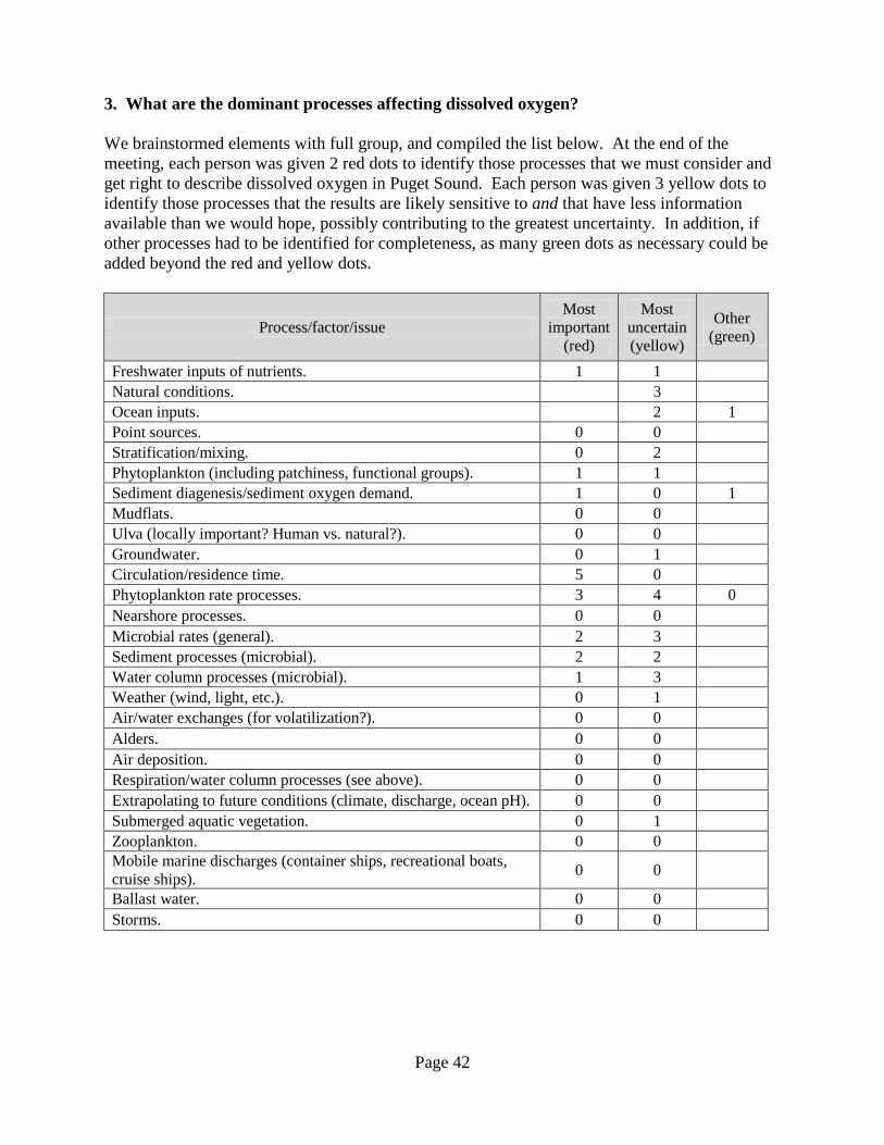
Page 42

3. What are the dominant processes affecting dissolved oxygen? We brainstormed elements with full group, and compiled the list below. At the end of the meeting, each person was given 2 red dots to identify those processes that we must consider and get right to describe dissolved oxygen in Puget Sound. Each person was given 3 yellow dots to identify those processes that the results are likely sensitive to and that have less information available than we would hope, possibly contributing to the greatest uncertainty. In addition, if other processes had to be identified for completeness, as many green dots as necessary could be added beyond the red and yellow dots.

Process/factor/issue Most

important (red)

Most uncertain (yellow)

Other (green)

Freshwater inputs of nutrients. 1 1 Natural conditions. 3 Ocean inputs. 2 1 Point sources. 0 0 Stratification/mixing. 0 2 Phytoplankton (including patchiness, functional groups). 1 1 Sediment diagenesis/sediment oxygen demand. 1 0 1 Mudflats. 0 0 Ulva (locally important? Human vs. natural?). 0 0 Groundwater. 0 1 Circulation/residence time. 5 0 Phytoplankton rate processes. 3 4 0 Nearshore processes. 0 0 Microbial rates (general). 2 3 Sediment processes (microbial). 2 2 Water column processes (microbial). 1 3 Weather (wind, light, etc.). 0 1 Air/water exchanges (for volatilization?). 0 0 Alders. 0 0 Air deposition. 0 0 Respiration/water column processes (see above). 0 0 Extrapolating to future conditions (climate, discharge, ocean pH). 0 0 Submerged aquatic vegetation. 0 1 Zooplankton. 0 0 Mobile marine discharges (container ships, recreational boats, cruise ships). 0 0

Ballast water. 0 0 Storms. 0 0

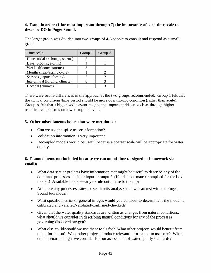
Page 43

4. Rank in order (1 for most important through 7) the importance of each time scale to describe DO in Puget Sound. The larger group was divided into two groups of 4-5 people to consult and respond as a small group.

Time scale Group 1 Group A Hours (tidal exchange, storms) 5 1 Days (blooms, storms) 4 1 Weeks (blooms, storms) 3 1 Months (neap/spring cycle) 1 2 Seasons (inputs, forcing) 2 2 Interannual (forcing, climate) 6 3 Decadal (climate) 7 3

There were subtle differences in the approaches the two groups recommended. Group 1 felt that the critical conditions/time period should be more of a chronic condition (rather than acute). Group A felt that a big episodic event may be the important driver, such as through higher trophic level controls on lower trophic levels. 5. Other miscellaneous issues that were mentioned:

• Can we use the spice tracer information? • Validation information is very important. • Decoupled models would be useful because a coarser scale will be appropriate for water

quality.

6. Planned items not included because we ran out of time (assigned as homework via email):

• What data sets or projects have information that might be useful to describe any of the dominant processes as either input or output? (Handed out matrix compiled for the box model.) Available models—any to rule out or rise to the top?

• Are there any processes, rates, or sensitivity analyses that we can test with the Puget Sound box model?

• What specific metrics or general images would you consider to determine if the model is calibrated and verified/validated/confirmed/checked?

• Given that the water quality standards are written as changes from natural conditions, what should we consider in describing natural conditions for any of the processes governing dissolved oxygen?

• What else could/should we use these tools for? What other projects would benefit from this information? What other projects produce relevant information to use here? What other scenarios might we consider for our assessment of water quality standards?

Page 44

Appendix B. Evaluation of Features of Hydrodynamic Model.

Model Features POM EFDC FVCOM ROMS CH3D GEMSS UnTRIM ADCIRC SELFE

Grid system Structured

(Quasi-curvilinear)

Structured (Quasi-

curvilinear)

US (Mesh: T)

Structured (Quasi-

curvilinear)

Structured (Curvilinear)

Structured (Quasi-

curvilinear)

US (Mesh:

OT,OQ)

US (Mesh: T)

US (Mesh: T,Q)

Dimension 3D 3D 3D 3D 3D 3D 3D 2D/3D 3D

Numerical method FDM FDM FVM FDM FDM FDM FDM & FVM FEM FEM

Vertical grid Sigma-grid Sigma-grid Sigma-grid S- coordinate Sigma-grid Z-grid Z-grid Z-grid Sigma-/ Z-grid

Equation Differential

(Mode splitting)

Differential (Mode

splitting)

Integral (Mode

splitting)

Differential (Mode

splitting)

Differential (Mode

splitting) N/A Differential

and integral

Integral with shape

function

Integral with shape

function

Wetting/Drying NO YES YES NO YES YES YES YES YES High-order transport schemes YES YES YES YES YES YES YES YES YES

Conservation YES YES YES YES YES YES YES NO NO

Meteorology force MMS MMS MMS/MMO MMO MMS MMS MMS MMS MMS Source code availability YES YES YES YES YES YES N/A YES YES

Application areas 3 3 3 3 3 2 2 3 2 Peer review of model theory 3 3 3 3 3 3 3 3 3

Technical documentation 3 3 3 2 2 2 2 2 2

Active development or user group

3 3 3 3 2 2 2 3 2

US: Unstructured, T: Triangle Mesh, Q: Quadrilateral Mesh, OT: Orthogonal Triangle Mesh, OQ: Orthogonal Quadrilateral Mesh, FDM: Finite Difference Method, FVM: Finite Volume Method, MMS: meteorology force from multiple stations, MMO: meteorological force from model output. Rating system: 3=excellent, 2=good, 1=can be adapted, 0 = not included.

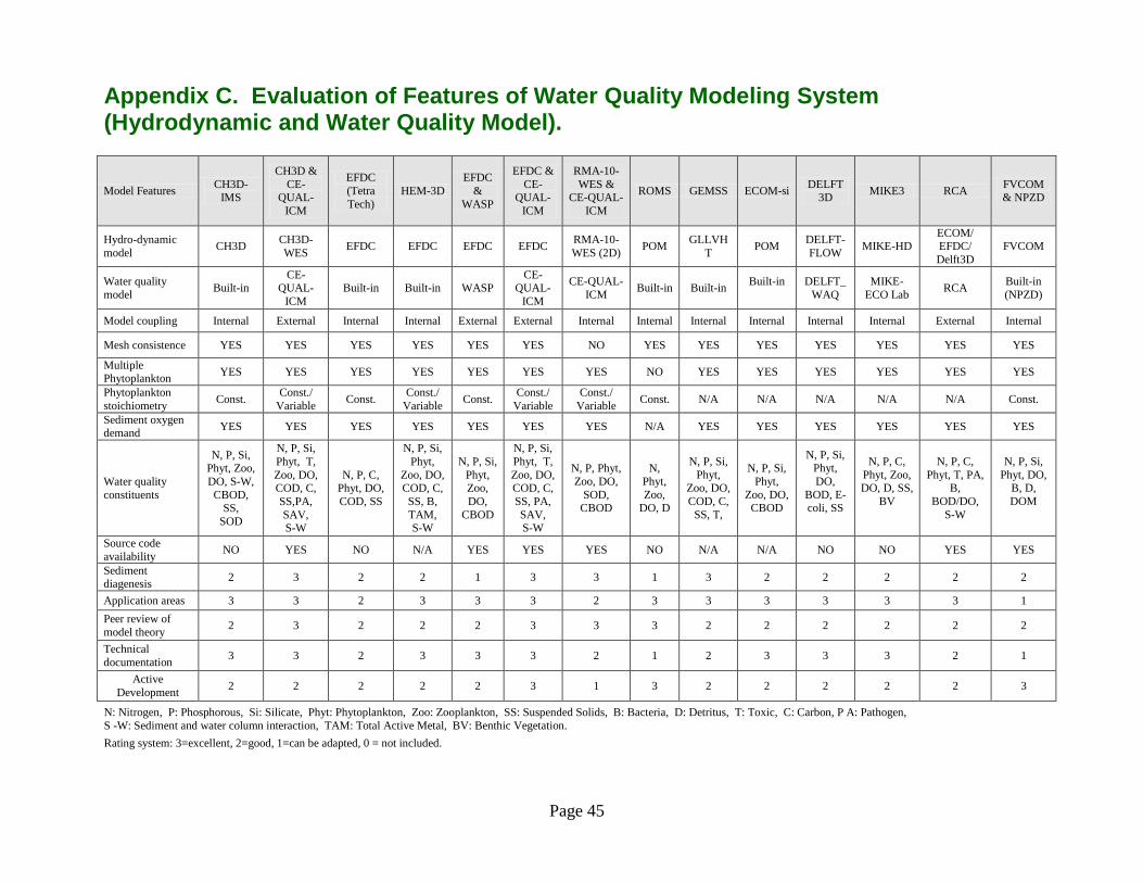
Page 45

Appendix C. Evaluation of Features of Water Quality Modeling System (Hydrodynamic and Water Quality Model).

Model Features CH3D-IMS

CH3D & CE-

QUAL-ICM

EFDC (Tetra Tech)

HEM-3D EFDC

& WASP

EFDC & CE-

QUAL-ICM

RMA-10-WES &

CE-QUAL-ICM

ROMS GEMSS ECOM-si DELFT 3D MIKE3 RCA FVCOM

& NPZD

Hydro-dynamic model CH3D CH3D-

WES EFDC EFDC EFDC EFDC RMA-10-WES (2D) POM GLLVH

T POM DELFT-FLOW MIKE-HD

ECOM/ EFDC/ Delft3D

FVCOM

Water quality model Built-in

CE-QUAL-

ICM Built-in Built-in WASP

CE-QUAL-

ICM

CE-QUAL-ICM Built-in Built-in Built-in

DELFT_

WAQ MIKE-

ECO Lab RCA Built-in (NPZD)

Model coupling Internal External Internal Internal External External Internal Internal Internal Internal Internal Internal External Internal

Mesh consistence YES YES YES YES YES YES NO YES YES YES YES YES YES YES

Multiple Phytoplankton YES YES YES YES YES YES YES NO YES YES YES YES YES YES

Phytoplankton stoichiometry Const. Const./

Variable Const. Const./ Variable Const. Const./

Variable Const./

Variable Const. N/A N/A N/A N/A N/A Const.

Sediment oxygen demand YES YES YES YES YES YES YES N/A YES YES YES YES YES YES

Water quality constituents

N, P, Si, Phyt, Zoo, DO, S-W, CBOD,

SS, SOD

N, P, Si, Phyt, T, Zoo, DO, COD, C, SS,PA, SAV, S-W

N, P, C, Phyt, DO, COD, SS

N, P, Si, Phyt,

Zoo, DO, COD, C, SS, B, TAM, S-W

N, P, Si, Phyt, Zoo, DO,

CBOD

N, P, Si, Phyt, T, Zoo, DO, COD, C, SS, PA, SAV, S-W

N, P, Phyt, Zoo, DO,

SOD, CBOD

N, Phyt, Zoo,

DO, D

N, P, Si, Phyt,

Zoo, DO, COD, C,

SS, T,

N, P, Si, Phyt,

Zoo, DO, CBOD

N, P, Si, Phyt, DO,

BOD, E-coli, SS

N, P, C, Phyt, Zoo, DO, D, SS,

BV

N, P, C, Phyt, T, PA,

B, BOD/DO,

S-W

N, P, Si, Phyt, DO,

B, D, DOM

Source code availability NO YES NO N/A YES YES YES NO N/A N/A NO NO YES YES

Sediment diagenesis 2 3 2 2 1 3 3 1 3 2 2 2 2 2

Application areas 3 3 2 3 3 3 2 3 3 3 3 3 3 1 Peer review of model theory 2 3 2 2 2 3 3 3 2 2 2 2 2 2

Technical documentation 3 3 2 3 3 3 2 1 2 3 3 3 2 1

Active Development 2 2 2 2 2 3 1 3 2 2 2 2 2 3

N: Nitrogen, P: Phosphorous, Si: Silicate, Phyt: Phytoplankton, Zoo: Zooplankton, SS: Suspended Solids, B: Bacteria, D: Detritus, T: Toxic, C: Carbon, P A: Pathogen, S -W: Sediment and water column interaction, TAM: Total Active Metal, BV: Benthic Vegetation. Rating system: 3=excellent, 2=good, 1=can be adapted, 0 = not included.

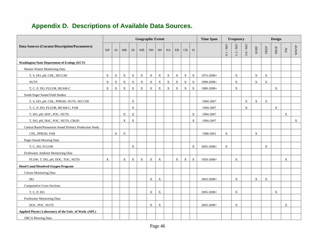
Page 46

Appendix D. Descriptions of Available Data Sources.

Data Sources (Curator/Description/Parameters)

Geographic Extent Time Span Frequency Design

SJF AI MB SS WB NH SH NA EB CB SI

0-1

/ MO

1-2

/ MO

3-6

/ MO

SUR

F

DEE

P

PRO

F

FW

WW

TP

Washington State Department of Ecology (ECY)

Marine Waters Monitoring Data

T, S, DO, pH, CHL, SECCHI X X X X X X X X X X X 1973-2008+ X X X

NUTS X X X X X X X X X X X 1999-2008+ X X X

T, C, P, DO, FLUOR, BEAM-C X X X X X X X X X X X 1989-2008+ X X

South Puget Sound Field Studies

T, S, DO, pH, CHL, PPROD, NUTS, SECCHI X 1994-2007 X X X

T, C, P, DO, FLUOR, BEAM-C, PAR X 1994-2007 X X

T, DO, pH, DOC, POC, NUTS X X X 1994-2007 X

T, DO, pH, DOC, POC, NUTS, CBOD X X X 1994-2007 X

Central Basin/Possession Sound Primary Production Study

CHL, PPROD, PAR X X 1998-2001 X X

Puget Sound Mooring Data

T, C, DO, FLUOR X X 2005-2008+ X X

Freshwater Ambient Monitoring Data

FLOW, T, DO, pH, DOC, TOC, NUTS X X X X X X X X X 1959-2008+ X X

Hood Canal Dissolved Oxygen Program

Citizen Monitoring Data

DO X X 2003-2008+ X X X

Comparative Cross Sections

T, C, P, DO X X 2005-2008+ X X

Freshwater Monitoring Data

DOC, POC, NUTS X X 2005-2008+ X X

Applied Physics Laboratory of the Univ. of Wash. (APL)

ORCA Mooring Data

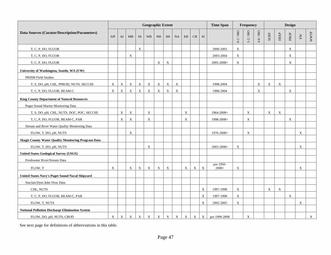
Page 47

Data Sources (Curator/Description/Parameters)

Geographic Extent Time Span Frequency Design

SJF AI MB SS WB NH SH NA EB CB SI

0-1

/ MO

1-2

/ MO

3-6

/ MO

SUR

F

DEE

P

PRO

F

FW

WW

TP

T, C, P, DO, FLUOR X 2000-2003 X X

T, C, P, DO, FLUOR X 2003-2004 X X

T, C, P, DO, FLUOR X X 2005-2008+ X X

University of Washington, Seattle, WA (UW)

PRISM Field Studies

T, S, DO, pH, CHL, PPROD, NUTS, SECCHI X X X X X X X X 1998-2004 X X X

T, C, P, DO, FLUOR, BEAM-C X X X X X X X X 1998-2004 X X

King County Department of Natural Resources

Puget Sound Marine Monitoring Data

T, S, DO, pH, CHL, NUTS, DOC, POC, SECCHI X X X X 1964-2008+ X X X

T, C, P, DO, FLUOR, BEAM-C, PAR X X X X 1998-2008+ X X

Stream and River Water Quality Monitoring Data

FLOW, T, DO, pH, NUTS X 1976-2008+ X X

Skagit County Water Quality Monitoring Program Data

FLOW, T, DO, pH, NUTS X 2003-2008+ X X

United States Geological Survey (USGS)

Freshwater River/Stream Data

FLOW, T X X X X X X X X X pre 1950-

2008+ X X

United States Navy's Puget Sound Naval Shipyard

Sinclair/Dyes Inlet Flow Data

CHL, NUTS X 1997-1998 X X X

T, C, P, DO, FLUOR, BEAM-C, PAR X 1997-1998 X X

FLOW, T, NUTS X 2002-2005 X X

National Pollution Discharge Elimination System

FLOW, DO, pH, NUTS, CBOD X X X X X X X X X X X pre 1999-2008 X X See next page for definitions of abbreviations in this table.

DEFINITIONS in Appendix D.

Measured Parameters T Temperature. S Salinity. C Conductivity (used to calculate salinity). P Pressure (used to calculate depth). DO Dissolved Oxygen concentrations estimated using Winkler titration method

(discrete samples) or electronic sensor (freshwater and profile data). CHL Chlorophyll a and phaeopigment concentrations estimated using standard acidification method. FLUOR Chlorophyll a concentration estimated from in vivo fluorescence. PPROD Phytoplankton primary production estimated from 14C uptake experiments.

NUTS Nutrient concentrations to include some combination of total and total dissolved nitrogen and phosphorous and separate estimates of dissolved NO3 (nitrate), NO2 (nitrite), NH4 (ammonium), PO4 (orthophosphate), and SiOH4 (silicate).

DOC Dissolved organic carbon. POC Particulate organic carbon. TOC Total organic carbon. pH Potential hydrogen. BEAM-C Light transmission. SECCHI Secchi disk measurement (surface only). PAR Photosynthetically available radiation (400-700 nm). CBOD Carbonaceous Biochemical Oxygen Demand. FLOW River/stream flow and effluent discharge. Geographic Extent SJF Strait of Juan de Fuca AI Admiralty Inlet MB Main Basin SS South Sound WB Whidbey Basin NH Northern Hood Canal SH Southern Hood Canal NA The Narrows EB Elliott Bay CB Commencement Bay SI Sinclair/Dyes Inlet Timespan/Frequency/Design SURF Discrete surface samples available. DEEP Discrete deep/near-bottom samples available. PROF Continuous vertical profile data available. FW Freshwater samples available. WWTP Waste water treatment plant samples available. + Ongoing data collection.

Page 49

Appendix E. Glossary, Acronyms, and Abbreviations. Ambient: Background or away from point sources of contamination.

Anoxic: Depleted of oxygen.

Anthropogenic: Human-caused.

Bathymetry: Measure of underwater depth of a waterbody.

Biotic: Produced or caused by living organisms.

Box model: A computer prediction tool to simulate the movement of water and pollutants within a waterbody.

Clean Water Act: A federal act passed in 1972 that contains provisions to restore and maintain the quality of the nation’s waters.

Diagenesis: Any chemical, physical, or biological change undergone by a sediment after its initial deposition.

Dissolved oxygen: A measure of the amount of oxygen dissolved in water

Eutrophication: An increase in productivity resulting from nutrient loads from human activities such as fertilizer runoff and leaky septic systems.

Hypoxia: Low oxygen

Loading: Quality of nutrients entering an ecosystem in a given period of time.

National Pollutant Discharge Elimination System (NPDES): National program for issuing, modifying, revoking and reissuing, terminating, monitoring, and enforcing permits, and imposing and enforcing pretreatment requirements under the Clean Water Act. The NPDES program regulates discharges from wastewater treatment plants, large factories, and other facilities that use, process, and discharge water back into lakes, streams, rivers, bays, and oceans.

Nonpoint source: Pollution that enters any waters of the state from any dispersed land-based or water-based activities, including but not limited to atmospheric deposition, surface water runoff from agricultural lands, urban areas, or forest lands, subsurface or underground sources, or discharges from boats or marine vessels not otherwise regulated under the National Pollutant Discharge Elimination System Program. Generally, any unconfined and diffuse source of contamination. Legally, any source of water pollution that does not meet the legal definition of “point source” in section 502(14) of the Clean Water Act.

Nutrient: Substance used by organisms to live and grow. Marine plant (algae or phytoplankton) growth often is limited by the nutrient, nitrogen.

Parameter: A measurable quantity that defines certain water quality characteristics of a system.

Point source: Sources of pollution that discharge at a specific location from pipes, outfalls, and conveyance channels to a surface water. Examples of point source discharges include municipal wastewater treatment plants, municipal stormwater systems, industrial waste treatment facilities, and construction sites that clear more than 5 acres of land.

Page 50

Acronyms and Abbreviations Following are acronyms and abbreviations used frequently in this report. BC British Columbia (Canada) BOD Biological oxygen demand DNR Department of Natural Resources Ecology Washington State Department of Ecology EPA U.S. Environmental Protection Agency MTAC Model Technical Advisory Committee NOAA National Oceanic Atmospheric Administration PAC Project Advisory Committee PNNL Pacific Northwest National Laboratory QA Quality assurance SJF Strait of Juan de Fuca SOD Sediment oxygen demand USGS U.S. Geological Survey WAC Washington Administrative Code WWTP Wastewater treatment plant