Quality Ratings and Premiums in the Medicare Advantage

Market

Ian M. McCarthy∗

Department of Economics

Emory University

Michael Darden†

Department of Economics

Tulane University

January 2015

Abstract

We examine the response of Medicare Advantage contracts to published quality ratings. We

identify the effect of star ratings on premiums using a regression discontinuity design that exploits

plausibly random variation around rating thresholds. We find that 3, 3.5, and 4-star contracts

in 2009 significantly increased their 2010 monthly premiums by $20 or more relative to contracts

just below the respective threshold values. High quality contracts also disproportionately dropped

$0 premium plans or expanded their offering of positive premium plans. Welfare results suggest

that the estimated premium increases reduced consumer welfare by over $250 million among the

affected beneficiaries.

JEL Classification: D21; D43; I11; C51

Keywords: Medicare Advantage, Premiums, Quality Ratings, Regression Discontinuity

∗Emory University, Rich Memorial Building, Room 306, Atlanta, GA 30322, Email: ian.mccarthy@Emory.edu†206 Tilton Memorial Hall, Tulane University, New Orleans, LA 70115. E-mail: mdarden1@tulane.edu

1

1 Introduction

The role of Medicare Advantage (MA) plans in the provision of health insurance to Medicare bene-

ficiaries has grown substantially. Between 2003 and 2014, the share of Medicare eligible individuals

in an MA health plan increased from 13.7% to 30%.1 To better inform enrollees of MA quality, in

2007, the Center for Medicare and Medicaid Services (CMS) introduced a five-star rating system that

provided a rating of one to five stars to each MA contract – a private organization that administers

potentially many differentiated plans – in each of five quality domains.2 For the 2009 enrollment

period, CMS began aggregating the domain level quality scores into an overall star rating for each

MA contract in which each plan offered by a contract would display the contract’s quality star rating.

Since in 2012, contracts have been incentivized to earn high quality star ratings through star-dependent

reimbursement and bonus schemes.

Early studies on the effects of the star rating program focus on the informational benefits to

Medicare beneficiaries. To this end, the program has been found to have a relatively small positive

effect on beneficiary choice, with heterogeneous effects across star ratings (Reid et al., 2013; Darden

& McCarthy, forthcoming). However, one area thus far overlooked concerns the supply-side response

to MA star ratings, where a natural consequence of the star rating program could be for contracts

to adjust premiums and other plan characteristics in response to published quality ratings.3 Indeed,

while the quality star program is often presented as a potential information shock to enrollees, the

program could also serve as an information shock to health insurance contracts, better informing them

of competitor quality and better informing contracts of their own signal of quality to the market. For

example, learning that its plans have the highest quality star rating in a market in 2009, a contract may

choose to price out its quality advantage in 2010 by raising plan premiums. Conversely, a relatively

low-rated contract may lower its 2010 premium in response to its 2009 quality star rating. More

generally, the extent to which policy may cause health insurance companies to adjust premiums is a

central question in health and public economics.4

The current paper provides a comprehensive analysis of 2010 premium adjustments to the 2009

publication of MA contract quality stars. We investigate the specific mechanisms by which contracts

can adjust their premiums in response to their quality ratings, and we calculate the corresponding wel-

fare effects. We adopt a regression discontinuity (RD) design that exploits plausibly random variation

around 2009 star thresholds, allowing us to separately identify the effect of reported quality on price

1Kaiser Family Foundation MA Update, available at http://kff.org/medicare/fact-sheet/medicare-advantage-fact-sheet/.

2For example, one domain on which contracts were rated was “Helping You Stay Healthy.”3Preliminary evidence of a supply-side response to the publication of MA quality stars was found in Darden &

McCarthy (forthcoming), albeit with a restricted sample of contract/plan/county/year observations.4For example, see Pauly et al. (2014) on the effects of the Affordable Care Act on individual insurance premiums.

2

from the overall relationship between quality and price. Our data on contract/plan market shares,

reported contract quality, plan premiums, and other plan characteristics come from several publicly

available sources. Our results suggest strong premium adjustments following the 2009 star rating pro-

gram, with average to above average star-rated contracts significantly increasing premiums from 2009

to 2010. When we conduct our analysis at the contract level, we find that 3, 3.5, and 4-star contracts

increase their average premiums across existing plans by $33.60, $29.30, $31.85, respectively, relative

to contracts with 2009 ratings just below the respective threshold values. At the plan level, we estimate

mean increases of $19.40, $41.99, and $31.52 for 3, 3.5, and 4-star contract/plans, respectively. These

effects are sizable compared to overall average premium increases of between $9 and $15. The results

are also broadly consistent across a range of sensitivity analyses, including consideration of alternative

bandwidths, falsification tests with counter-factual threshold values, and the exclusion of market-level

covariates.

While an MA contract may directly adjust its plans’ premiums in response to quality stars, the

contract may also adjust the mix of plans it offers within a market (county). For example, in response

to the published star ratings, a contract could alter the number of zero-premium plans; adjust the

number of plans that include Medicare Part D coverage; change the drug deductible in plans that offer

part D coverage; or add/drop plans entirely. Indeed, our data show that nearly all of the regional

variation in plan premiums is due to selection of plan offerings by contracts, as opposed to contracts

charging different premiums in different areas of the country. We find that contracts just above the

3 and 3.5-star thresholds in 2009 are more likely to drop $0 premium plans in 2010, with 3.5-star

contracts also more likely to introduce positive premium plans into new markets. We find no such

disproportionate change in $0 or positive premium plans among contracts with a 4-star rating in 2009.

Meanwhile, low quality contracts (those just above the 2.5-star threshold in 2009) maintain their 2009

plan offerings at largely the same premium levels in 2010, while contracts just below the 2.5-star

threshold in 2009 are much more likely to exit the market altogether in 2010.

Overall, our results suggest that the star rating program in 2009 may have caused low quality

contracts to drop plans while generating large premium increases among contracts receiving 3-star

ratings and above. Adopting the consumer welfare calculations used in Town & Liu (2003) and

Maruyama (2011), our estimated increases in premiums imply a reduction in consumer surplus of over

$250 million among those beneficiaries enrolled in the relevant plans. To the extent that higher quality

plans are replacing low quality plans at reasonable premium levels, plan entry and exit behaviors

induced by the star-rating program may partially offset this welfare loss; however, given the number of

new plans estimated to have entered the market due to the star ratings, such offsets are likely relatively

small (Maruyama, 2011).

3

In what follows, we discuss the institutional details of Medicare Advantage and the recent star

rating program in Section 2. The data and methods are discussed in Sections 3 and 4, respectively.

We present our results in Section 5, with a series of robustness checks discussed in Section 6. Section

7 examines the potential mechanisms underlying our estimated premium adjustments, and Section 8

summarizes the welfare effects associated with our estimated premium increases. The final section

concludes.

2 Institutional Background

Since Medicare’s inception, beneficiaries have had the option to receive benefits through private health

insurance plans. The Balanced Budget Act of 1997 (BBA) classified all private Medicare health insur-

ance plans as Medicare Part C plans, and it allowed for additional types of business models including

Preferred Provider Organizations (PPOs), Provider-Sponsored Organizations (PSOs), Private fee-for-

service (PFFS) plans, and Medical Savings Accounts (MSAs). Later, in addition to the beneficiary

entitlement to prescription drug coverage, the Medicare Modernization Act of 2003 renamed Medi-

care Part C plans as Medicare Advantage (MA) plans. In each year since 2003, Medicare beneficiaries

choose to enroll in traditional fee-for-service (FFS) Medicare or an MA plan during an open enrollment

period from November 1st through December 31st. By enrolling in an MA plan, enrollees must pay

Medicare Part B premiums in addition to any additional premium charged by the plan. In exchange,

MA plans provide at least (often more than) the services covered by traditional FFS Medicare. In

2009, 38% of MA plans charged no additional premium, while 77% of plans also offered prescription

drug coverage. Given the generosity of plan coverage at possibly no additional cost relative to tradi-

tional Medicare FFS, the MA has grown dramatically in recent years with share of Medicare eligible

individuals in an MA plan increasing from 13.7% in 2003 to 30% in 2014.5

Broadly, an MA contract is an agreement between a private insurance company and CMS whereby

the company agrees to insure Medicare beneficiaries in exchange for reimbursement. A contract is

approved by CMS to operate in specific counties, and an approved contract typically offers a menu

of MA plans that are differentiated by premium, prescription drug coverage, and, if covered, the

prescription drug deductible. Most MA contracts are required to offer at least one plan that includes

prescription drug coverage. For the 2015 enrollment year, 78% of all Medicare beneficiaries live in a

county with access to at least one plan that offers prescription drug coverage (MA-PD) and charges no

additional premium (above the Part B premium).6 In 2009, the mean number of MA plans available to

5Kaiser Family Foundation MA Update, available at http://kff.org/medicare/fact-sheet/medicare-advantage-fact-sheet/.

6http://kff.org/medicare/issue-brief/medicare-advantage-2015-data-spotlight-overview-of-plan-changes/

4

beneficiaries was roughly 11 plans per county.7 However, there exists considerable regional variation in

the availability of MA plans, and enrollments in MA plans are concentrated in a few national contracts.

Indeed, according to the Kaiser Family Foundation (KFF), 60% of all plans offered in 2015 are affiliated

with just seven health insurance companies.8

Staring in the 2007 enrollment year, CMS began collecting and distributing a one to five-star

quality rating in each of five quality domains (e.g., “Helping You Stay Healthy”). Each domain

was itself an aggregation of many individual quality metrics such as the percentage of enrollees with

access to an annual flu vaccine. These individual quality metrics are calculated based on data from a

variety of sources, including HEDIS, the Consumer Assessment of Healthcare Providers and Systems

(CAHPS), the Health Outcomes Survey (HOS), the Independent Review Entity (IRE), the Complaints

Tracking Module (CTM), and CMS administrative data. Starting in enrollment year 2009, CMS began

aggregating the domain level quality stars to an overall contract rating of between one and five stars

(in half-star increments).9 And since 2011, CMS constructs the contract-specific quality ratings as a

function of Part D coverage, when relevant. Our focus is on the 2009 and 2010 enrollment years -

the first two years of the overall contract star rating program and the years in which all contracts,

including those offering prescription drug coverage, were rated based on the same underlying quality

metrics.

The literature on the MA quality rating initiatives has generally focused on the enrollment effects.

Recently, Reid et al. (2013) find large effects of increases in star-ratings on enrollment that are homo-

geneous across the reported quality distribution, but results from that paper fail to disentangle the

effects of quality from quality reporting on enrollment. Attempting to disentangle these effects, Darden

& McCarthy (forthcoming) find heterogeneous effects of the quality star rating program on MA plan

enrollment in 2009 and no significant effect in 2010. At the plan level, they find that a marginally

higher rated contract at the lower end of the quality distribution (e.g., a 3 as compared to 2.5 starred

contract) realized a positive and significant enrollment effect equal to 4.75 percentage points relative

to traditional FFS Medicare in 2009 enrollments. This effect diminishes for higher rated contracts,

and vanishes for the 2010 enrollment year. The lack of an enrollment response to 2010 quality stars

suggests that the 2009 star ratings may have acted as a one-time informational event, or that there

was a supply-side response in 2010 based on the 2009 ratings.

Generally, the potential for supply-side responses to Medicare Advantage policy has received little

attention from researchers. One recent exception is Stockley et al. (2014), who examine how MA plan

premiums and benefits respond to variation in the benchmark payment rate - the subsidy received

7Author’s calculation. See Section 3 for a presentation of our data.8See http://kff.org/medicare/issue-brief/medicare-advantage-2015-data-spotlight-overview-of-plan-changes/.9For a complete discussion of the star rating program, see Darden & McCarthy (forthcoming).

5

by the MA contract for each enrollee. Those authors find that contracts do not adjust premiums

directly as a result of changes in benchmark payment rates, but rather contracts adjust the generosity

of plan benefits in response. Conversely, Darden & McCarthy (forthcoming) find that contract/plans

in 2010 raise premiums in response to higher 2009 contract-level quality star ratings. However, the

sample used to estimate the supply-side response of contracts in 2010 was restricted to just those

contract/plans with a.) 10 or more enrollees in both 2009 and 2010 and b.) nonmissing quality ratings

in 2010. Furthermore, that paper only focuses on direct premium increases, ignoring the possibility

of indirect premium adjustments such as changing the number of zero-premium plans or adjust the

plan-mix within a county. The current paper provides a comprehensive examination of the supply-side

response to quality star ratings, examining the full population of approved MA contracts to evaluate

several potential response mechanisms as well as potential welfare consequences.

3 Data

We collect data on market shares, contract/plan characteristics, and market area characteristics from

several publicly available sources for calendar years 2009 and 2010.10 As a base, we use the Medicare

Service Area files to form a census of MA contracts that were approved to operate in each county

in the United States in 2009 and 2010. To these contract/county/year observations, we merge con-

tract/plan/county/year data on enrollment and other contract characteristics.11 To our market share

data, we merge further information on MA contract quality ratings, contract/plan premiums, county-

level MA market share, CMS benchmark rates, fee-for-service costs, hospital discharges, and census

data. The CMS quality information includes an overall summary star measure; star ratings for differ-

ent domains of quality (e.g., helping you stay healthy); as well as star ratings and continuous summary

scores for each individual metric (e.g., percentage of women receiving breast cancer screening and an

associated star rating). Data are not available for the overall continuous summary score (i.e., the score

rounded to generate an overall star rating), but we are able to replicate this variable by aggregating the

specific quality measures following CMS instructions. We explain this process thoroughly in Appendix

B. Hospital discharge data are from the annual Hospital Cost Reporting Information System (HCRIS),

and CMS benchmark rates and average FFS costs by county are publicly available from CMS. Finally,

county-level demographic and socioeconomic information are from the American Community Survey

(ACS).

10See Appendix C for a detailed discussion of our dataset and specific links.11CMS suppresses enrollment counts for contract/plans with 10 or fewer enrollees, but we keep these observations and

impute enrollment. The Service Area files are needed because the enrollment files do not account for migration. Forexample, it is possible for the enrollment file to contain a positive enrollment record for a contract/plan in a county evenif that contract is not approved to operate in the county. See Appendix C for futher details.

6

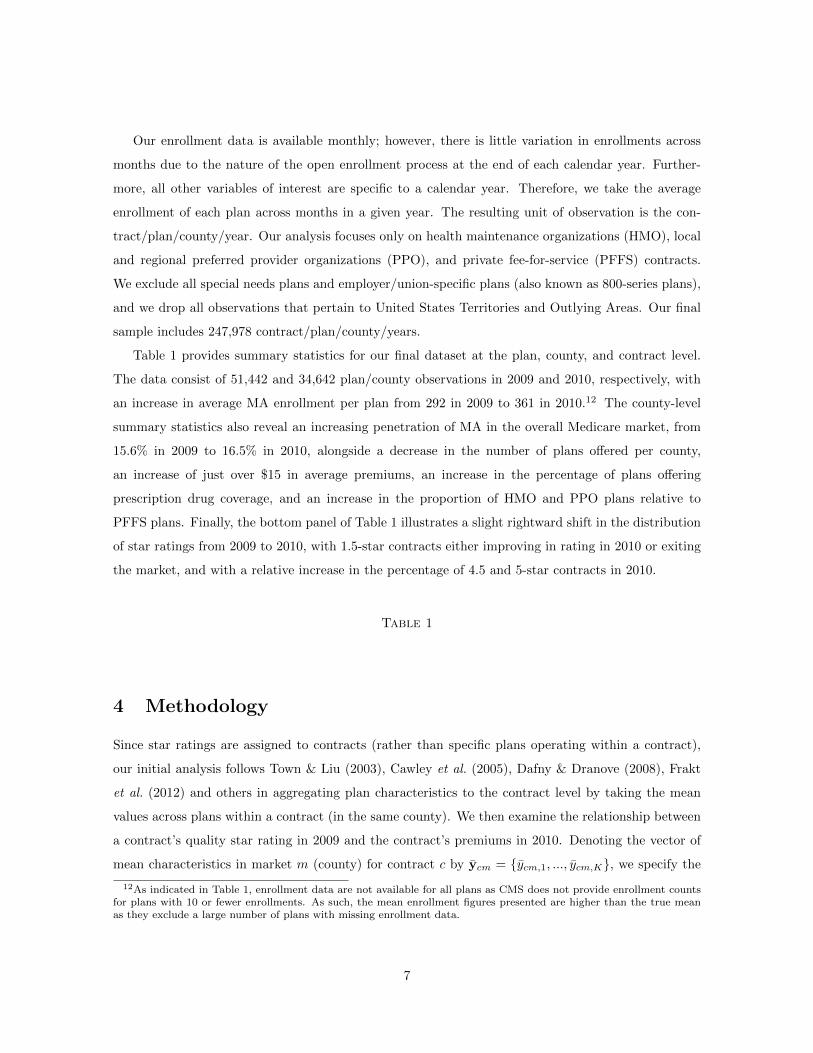
Our enrollment data is available monthly; however, there is little variation in enrollments across

months due to the nature of the open enrollment process at the end of each calendar year. Further-

more, all other variables of interest are specific to a calendar year. Therefore, we take the average

enrollment of each plan across months in a given year. The resulting unit of observation is the con-

tract/plan/county/year. Our analysis focuses only on health maintenance organizations (HMO), local

and regional preferred provider organizations (PPO), and private fee-for-service (PFFS) contracts.

We exclude all special needs plans and employer/union-specific plans (also known as 800-series plans),

and we drop all observations that pertain to United States Territories and Outlying Areas. Our final

sample includes 247,978 contract/plan/county/years.

Table 1 provides summary statistics for our final dataset at the plan, county, and contract level.

The data consist of 51,442 and 34,642 plan/county observations in 2009 and 2010, respectively, with

an increase in average MA enrollment per plan from 292 in 2009 to 361 in 2010.12 The county-level

summary statistics also reveal an increasing penetration of MA in the overall Medicare market, from

15.6% in 2009 to 16.5% in 2010, alongside a decrease in the number of plans offered per county,

an increase of just over $15 in average premiums, an increase in the percentage of plans offering

prescription drug coverage, and an increase in the proportion of HMO and PPO plans relative to

PFFS plans. Finally, the bottom panel of Table 1 illustrates a slight rightward shift in the distribution

of star ratings from 2009 to 2010, with 1.5-star contracts either improving in rating in 2010 or exiting

the market, and with a relative increase in the percentage of 4.5 and 5-star contracts in 2010.

Table 1

4 Methodology

Since star ratings are assigned to contracts (rather than specific plans operating within a contract),

our initial analysis follows Town & Liu (2003), Cawley et al. (2005), Dafny & Dranove (2008), Frakt

et al. (2012) and others in aggregating plan characteristics to the contract level by taking the mean

values across plans within a contract (in the same county). We then examine the relationship between

a contract’s quality star rating in 2009 and the contract’s premiums in 2010. Denoting the vector of

mean characteristics in market m (county) for contract c by ycm = {ycm,1, ..., ycm,K}, we specify the

12As indicated in Table 1, enrollment data are not available for all plans as CMS does not provide enrollment countsfor plans with 10 or fewer enrollments. As such, the mean enrollment figures presented are higher than the true meanas they exclude a large number of plans with missing enrollment data.

7

mean characteristic k for contract c as follows:

ycmk = f (qc, Xcm,Wm) + εcmk, (1)

where qc denotes the contract’s star rating in 2009, Xcm denotes other contract characteristics, Wm

denotes 2010 market-level data on the age, race, and education profile of a given county, and εcmk

is an error term independently distributed across characteristics and markets.13 Given our focus on

premiums, our plan characteristics of interest consist of the average premium and the proportion of

the contract’s plans (in the same county) charging a $0 premium.14

The CMS quality rating system relies on a continuous summary score between 1 and 5 which is

rounded to the nearest half. A contract with a 2.24 summary score is therefore rounded down to a 2-star

rating, while a contract with a 2.26 summary score is rounded up to a 2.5-star rating. Intuitively, these

two contracts are essentially identical in quality but received different quality ratings. We propose to

exploit the nature of this rating system using a regression discontinuity (RD) design.15 More formally,

denote by Rc the underlying summary score, by R the threshold summary score at which a new star

rating is achieved (e.g., R = 2.25 when considering the 2.5 star rating), and by Rc = Rc − R the

amount of improvement necessary to achieve an incremental improvement in rating. We then limit our

analysis to contracts with summary scores within a pre-specified bandwidth, h, around each respective

threshold value, R. For example, to analyze the impact of improving from 2.0 to 2.5 stars, the sample

is restricted to contracts with summary scores of 2.25 ±h.

To implement our approach, we specify plan/contract quality as follows:

qc = γ1 + γ2 × I(Rc > R

)+ γ3 × Rc + γ4 × I

(Rc > R

)× Rc, (2)

where γ2 is the main parameter of interest. Incorporating this RD framework into equation (1), and

adopting a linear functional form for f(.), yields the final regression equation

yckm = γ1 + γ2 × I(Rc > R

)+ γ3 × Rc + γ4 × I

(Rc > R

)× Rc

+βcXcm + βmWm + εckm, (3)

where Wm and Xcm are as discussed previously. Our baseline analysis estimates equation 3 using

ordinary least squares with a bandwidth of h = 0.125. We consider alternative bandwidths in Section

13We cluster standard errors by contract; however, the results are qualitatively unchanged when clustering standarderrors at the county level.

14The overall plan type (e.g., HMO versus PPO) is typically contract-specific and therefore does not vary across planswithin the same contract.

15See Imbens & Lemieux (2008) for a detailed discussion of the RD design and its application in economics.

8

6 as well as a more traditional RD design with a triangular kernel Imbens & Lemieux (2008).

Changes in mean premiums at the contract level can arise in several ways, most directly via changes

to premiums among specific plans. To investigate this possibility, we also estimate a regression of 2010

plan premiums as a function of the plans’ 2009 premiums, 2009 star ratings and other contract-level

variables, and 2009 county characteristics. This analysis is akin to estimating equation 3 but where

our analysis is at the plan level rather than aggregating to the contract level. For this analysis, we

examine only plans that were available in the same county in both 2009 and 2010.

5 Results

5.1 Average Premiums at the Contract Level

Table 2 presents the results of a standard OLS regression of mean contract characteristics in 2010

on the 2009 mean value, the contract’s 2009 star rating, as well as additional county and contract-

level covariates. To the extent that contract quality is already reflected in the contract’s mean plan

characteristics, we would expect the effects of increasing star ratings to be relatively small in magnitude.

This is the case in Table 2, where we see small decreases in average premiums among 2.5 and 4-star

contracts with small increases in premiums among 3 and 3.5-star contracts (relative to contracts with

one-half star lower ratings). Note that, in order to better reflect the premium charged to a given

enrollee in a specific contract, our analysis of average premiums at the contract level excludes plans

with 10 or fewer enrollments.16 Our analysis at the plan-level makes no such exclusion.

Table 2

The OLS results say little about the specific effects of an increase in reported quality on premiums.

To address this question directly, Table 3 presents the initial RD results at the contract level for a

bandwidth of h = 0.125. The results suggest a large premium increase for contracts receiving a 3, 3.5,

or 4 star rating in 2009, with these contracts increasing average premiums by between $29 and $34

per month from their 2009 levels relative to contracts with one-half star lower ratings. By contrast,

contracts receiving a 2.5-star rating showed no statistically significant increase in premiums. By virtue

of the RD design and the nature of the CMS star rating program, we argue that these estimates can be

interpreted as the causal effect of a one-half star increase in quality ratings separate from the quality

16Not surprisingly, low star-rated plans with 10 or fewer enrollments also charge much higher premiums relative tothe same quality plans with higher enrollments. For example, in 2010, the average premium among 2.5-star plans with10 or fewer enrollments was $63, compared to just $32 among 2.5-star plans with 11 or more enrollments. The resultsare nonetheless consistent when we include all plans and an indicator variable for missing enrollment data.

9

of the contract itself. For example, 3.5-star contracts of comparable “true” quality to 3-star contracts

were able to increase their premiums on average $29 per month. Looking purely at sample averages,

all other contracts receiving a 3.5-star rating in 2009 increased their premiums by an average of $12,

while 3-star contracts falling just below the 3.25 threshold increased their premiums by just over $3.

We provide extensive robustness and sensitivity analyses for these results in Section 6.

Table 3

5.2 Premiums at the Plan Level

Table 4 summarizes the RD results for 2010 plan premiums as a function of 2009 premiums, county-

level covariates, as well as the contract’s quality rating as specified in equation 2. This analysis

therefore estimates premium changes at the plan level (for the same plans offered in both 2009 and

2010), rather than analyzing average premiums at the contract level as in Table 3. For the same

plan/county/contract, the results again show a large and statistically significant increase in premiums

for 3, 3.5, and 4-star contracts, with premiums increasing by between $19 and $42 per month for the

same plans.

Table 4

6 Robustness and Sensitivity Analysis

The appropriateness of our proposed RD design depends critically on whether contracts can sufficiently

adjust their summary scores. Intuitively, it is unlikely that contracts can manipulate their scores

because the star ratings are calculated based on data two or three years prior to the current enrollment

period. Contracts would therefore not have the opportunity to manipulate other observable plan

characteristics in response to their same-year star ratings. To test this formally, McCrary (2008)

proposes a test of discontinuity in the distribution of summary scores around the threshold values.

The resulting t-statistics range from 0.15 to 0.96, suggesting no evidence of a discontinuity in the

running variable at any of the threshold values. In the remainder of this section, we investigate the

sensitivity of our results along several other dimensions, including: 1) bandwidth selection; 2) inclusion

of covariates; and 3) falsification test with counter-factual threshold values.

10

6.1 Choice of Bandwidth

The choice of bandwidth is a common area of concern in the RD literature (Imbens & Lemieux, 2008;

Lee & Lemieux, 2010). To assess the sensitivity of our results to the choice of bandwidth, we replicated

the local linear regression analysis from Tables 3 and 4 for alternative bandwidths ranging from 0.1 to

0.25 in increments of 0.005. The results for mean plan premiums at the contract level (Table 3) are

illustrated in Figure 1, where each graph presents the estimated star-rating coefficient, γ2, along with

the upper and lower 95% confidence bounds. Similar results for plan-level premium adjustments are

presented in Figure 2. In general, our results are consistent across a range of alternative bandwidths.

Figure 1

6.2 Inclusion of Covariates

The RD literature generally advises against including covariates in a standard RD design (Imbens

& Lemieux, 2008; Lee & Lemieux, 2010). The intuition for this advice is as follows: if treatment

assignment is random within the relevant bandwidth, then the covariates should also be randomly

assigned to the treated and control groups. However, in our setting, purely randomized quality scores

at the contract level would not necessarily imply randomization in county-level variables. As such, we

argue that county-level covariates belong in our analysis in order to control for geographic variation

influencing contract location and plan offerings.

Nonetheless, we assess the sensitivity of our analysis to the exclusion of these covariates by estimat-

ing a more traditional RD model with right-hand side variables presented in equation 2. We estimate

the effect of a one-half star increase in quality ratings with a triangular kernel and our preferred

bandwidth of h = 0.125. The results, summarized in Table 8, are generally consistent with our initial

findings in Tables 3 and 4, where we again see large increases in average premiums among 3, 3.5, and

4-star contracts relative to contracts just below the respective star-rating thresholds. One exception is

the estimated effect on individual plan premiums for 4-star versus 3.5-star contracts presented in the

bottom right of Table 8. In this case, unlike the estimates in Table 4, we find no significant increase

in premiums among 4-star contracts along with a reduction in the magnitude of the estimated effect.

This is perhaps not surprising given the location of higher rated contracts throughout the country,

where 4-star contracts are more concentrated in specific geographic areas relative to lower star-rated

contracts.

11

Table 8

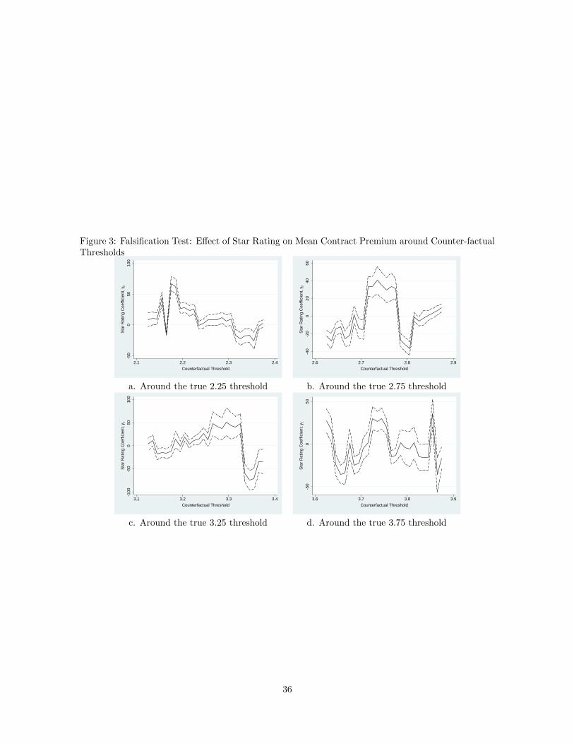
6.3 Falsification Tests

Finally, it is possible that the observed jumps at threshold values of 2.25, 2.75, etc. are driven more by

specific contracts that happen to fall above or below the threshold versus the star rating system itself.

As a test, we therefore considered a series of counter-factual threshold values above and below the

true threshold values. Intuitively, we should not see any jumps in premiums around these thresholds.

Figure 3 presents the results of this analysis for mean premiums at the contract/county level, where

we estimated the effects just as we did for Figure 1 and Table 3. The results support 2.75 and 3.25 as

the true threshold values, with the largest premium increases occurring just above those thresholds.

The results for 2.25 and 3.75 thresholds are less conclusive, with apparent jumps in premiums for what

should be irrelevant thresholds such as 1.9, 3.65, and 3.85.

Figure 3

7 Mechanisms for Premium Adjustment

Comparing our contract-level (Table 3) and plan-level (Table 4) analysis, we see larger premium

increases at the plan level for 3.5-star contracts and smaller increases at the plan level for 3-star

contracts. These results suggest that increases in average premiums at the contract level do not arise

solely from increases in premiums of the same plans from 2009 to 2010. Rather, the results suggest that

contracts also alter their plan mix from one year to the next (e.g., dropping plans within a contract,

introducing new plans under the same contract, or expanding plans to new counties).

Table 5 summarizes the exit behaviors from 2009 to 2010 by star rating, where we see low quality

plans were significantly more likely to exit their respective markets than plans associated with higher

star ratings. In particular, we see almost all 1.5-star plans leave the market from 2009 to 2010, with

very little exit among 4 and 4.5-star plans.17 Regarding plan entry, Table 5 shows that of the contracts

receiving a 1.5-star rating in 2009 that still operate in 2010, 37% of the underlying plans entered into a

new county in 2010. Similarly, 55% of 2-star plans (in 2009) entered into a new county in 2010, while

higher rated contracts were relatively less likely to enter into new markets. Collectively, the exit and

17The 1.5-star contracts that stayed in the market from 2009 to 2010 also had a marginally higher star rating in 2010.As such, there are no 1.5-star contracts remaining in 2010 (see Table 1).

12

entry figures reflect larger turnover in plan offerings among lower rated contracts relative to higher

rated contracts. This is perhaps expected as higher rated contracts may be more deliberate in their

market entry/exit decisions and less likely to quickly cycle through new plans from one year to the

next.

Table 5

7.1 Analysis of Plan Exit

To examine plan exit more directly, we follow Bresnahan & Reiss (1991), Cawley et al. (2005), Abraham

et al. (2007), and others in assuming that an insurance company will only offer a plan in a given county

if the plan positively contributes to the contract’s profit. Assuming profit is additively separable across

geographic markets (counties), our observed plan choice indicator becomes:

yc(j)m =

1 if πc(j)m = g(Wm, Xc(j)m

)+ εc(j)m ≥ 0

0 if πc(j)m < 0

(4)

where Wm again denotes county-level demographics, Xc(j)m denotes contract and plan characteristics

(including the contract’s 2009 quality, qc, plan premium, Part D participation, etc.), and εc(j)m is an

error term independently distributed across markets and plans.

We adopt a reduced form, linear profit specification with covariates including the benchmark CMS

payment rates, 2009 contract quality (qc), the plan’s enrollments in 2009, the number of physicians

in the county, the average Medicare FFS cost per beneficiary in the county, and plan characteristics

such as premiums, whether the plan offers prescription drug coverage, and indicators for HMO or PPO

plan type. Within this specification, we also consider the RD design from equation 2. We estimate

equation 4 with a linear probability model where yc(j)m = 1 indicates that the contract continued to

offer the plan in 2010 and yc(j)m = 0 indicates the plan was dropped. By definition, this analysis is

based on existing plans as of 2009.

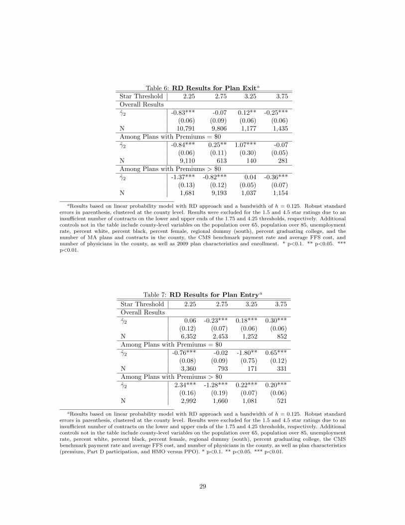
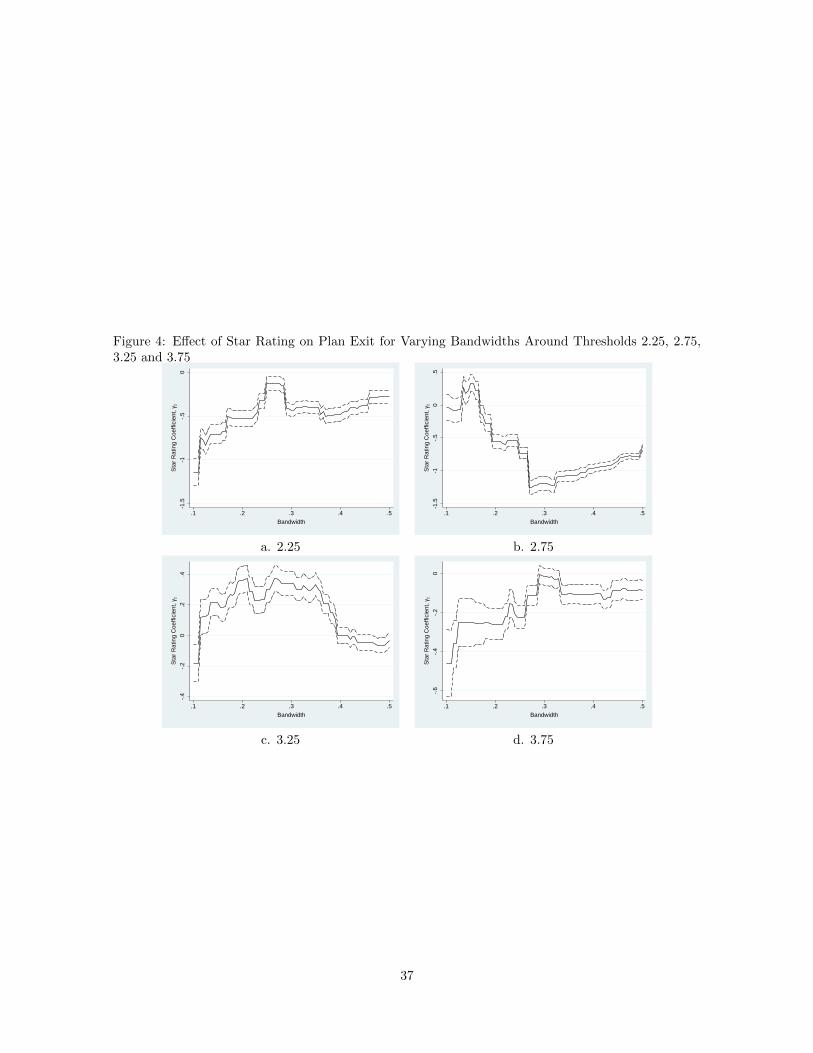
The results of our RD analysis of plan exit are summarized in Table 6. The top panel presents

results for all plans, while the remaining panels present results for plans with $0 premiums and plans

with positive premiums, respectively. Overall, we see that 2.5-star contracts are significantly less likely

to exit markets than 2-star contracts of similar overall quality. Relative to 2.5-star contracts, 3-star

contracts show no significant differences in exit behaviors, but they are significantly more likely to

drop their $0 premium plans and less likely to drop positive premium plans. Somewhat surprisingly,

13

contracts receiving a 3.5-star rating are more likely to drop plans overall; however, from the middle

panel of Table 6, we see that this result is entirely driven by 3.5-star contracts dropping their $0

premium plans. Finally, 4-star contracts are significantly less likely to exit overall, particularly for

their positive premium plans.18

Table 6

7.2 Analysis of Plan Entry

An important and relatively unique aspect of the MA market concerns the distinction between plan

and contract-level decisions. Specifically, contracts must obtain CMS approval in order to be offered

in a given county; however, conditional on receiving CMS approval, the decision of which plan(s) to

offer in a county is relatively less regulated. As a result, we argue that the fixed costs of entry are

primarily incurred at the contract level while the plan-level entry/exit decisions are based on the vari-

able profits per enrollee (i.e., regardless of market share). With regard to plan entry, this unique CMS

approval process alleviates many of the traditional econometric issues surrounding multiple equilibria

or endogeneity of other players’ actions in models of market entry with incomplete information (Berry

& Reiss, 2007; Bajari et al., 2010; Su, 2012). Conditional on plan characteristics, our entry analysis

therefore need only consider variable cost shifters and should be largely independent of the number or

type of competing plans in the county.19

The full set of plans available to a contract in a given market m is identified by taking all plans

offered under that contract across the entire state in the same year. All such plans are therefore

considered “eligible” to be operated in any given county, and the contract must choose which of those

plans to offer in each county, where yc(j)m = 1 indicates that the plan was added to the county (under

that contract) in 2010, and yc(j)m = 0 indicates that the plan was not offered. As with our analysis

of plan exit, we estimate the entry-equivalent to equation 4 using a standard linear probability model,

with entry considered as a function of 2010 county and plan characteristics as well as 2009 contract

quality as in equation 2.

Table 7 summarizes the results of our RD analysis for plan entry. Note that these results only

apply to markets in which the contracts previously operated (i.e., we do not consider the contract-level

18The robustness of our plan exit results to bandwidth selection is summarized in Appendix D. The overall results (toppanel of Table 6) at the 2.75 threshold appear relatively sensitive to bandwidth selection, with the statistical significance,magnitude, and sign of the point estimates changing within bandwidths from 0.1 to 0.2. In terms of hypothesis testing,we interpret this as evidence in favor of the null that the star rating has no effect on plan exit at the 2.75 threshold. Assuch, the qualitative findings from our point estimates in Table 6 are unchanged.

19Results are robust when we weaken this assumption and allow predicted 2010 market shares to influence entrybehaviors. The results are excluded for brevity but available upon request.

14

entry decisions and instead focus specifically on the plan-level entry of pre-existing contracts). The RD

results indicate that a one-half star improvement for 3 or 3.5-star contracts makes them significantly

more likely to expand their plans into new markets. The bottom panels of Table 7 further reveal that

the increase in probability of plan entry occurs for the positive premium plans, with 3.5-star contracts

significantly less likely to enter new markets with their $0 premium plans.20

Table 7

8 Welfare Effects

To examine the welfare effects of our estimated premium increases in Section 5, we follow Town &

Liu (2003) and Maruyama (2011) in estimating a standard Berry-type model of plan choice based on

market-level data (Berry, 1994). Specifically, let the utility of individual i from selecting Medicare

option c(j) in market area m be given as

Uic(j)m = δc(j)m + ξc(j)m + ζig + (1− σ)εic(j)m, (5)

where δc(j)m and ξc(j)m represent the mean level of utility derived from observed and unobserved

contract-plan-market area characteristics, respectively. We include in δc(j)m observed characteristics at

the contract and plan level, including premiums, plan type (HMO, PPO, or PFFS), and the underlying

summary score of the contract. Similar to Town & Liu (2003), we partition the set of Medicare options

into two groups: 1) MA plans that offer prescription drug coverage (MA-PD plans); and 2) MA plans

that do not offer prescription drug coverage (MA-Only). Traditional Medicare FFS is taken as our

outside option.

In addition to the i.i.d. extreme value error εic(j)m, individual preferences are allowed to vary

through group dummies ζig. This nested logit structure relaxes the independence of irrelevant al-

ternatives assumption and allows for differential substitution patterns between nests. The nesting

parameter, σ, captures the within-group correlation of utility levels.

Following Berry (1994) and others, the parameters in equation 5 can be estimated using market-

level data on the relative share of MA plans. Specifically, our estimation equation is as follows:

ln(Sc(j)m)− ln(S0m) = xc(j)mβ − αFc(j) + σln(Sc(j)m|g) + ξc(j)m, (6)

20The robustness of our plan entry results to bandwidth selection is summarized in Appendix D.

15

where xc(j)m denotes observed plan/contract characteristics, and ξc(j)m denotes the mean utility de-

rived from unobserved plan characteristics. We estimate the parameters of equation 6 using two-stage

least squares (2SLS) due to the endogeneity of within-group shares, Sc(j)m|g, and plan premiums, Fc(j).

We take as instruments the number of contracts operating in a county, the number of hospitals in a

county, the Herfindahl-Hirschman Index (HHI) for hospitals in a county (based on discharges), and

the number of physicians in the county. The results of this regression are presented in Appendix D.

With estimates of the mean observed utility, δc(j)m, and the within-group correlation, σ, estimated

monthly consumer surplus for a representative MA beneficiary is then derived as follows (Manski &

McFadden, 1981; Town & Liu, 2003; Maruyama, 2011):

Wi =1

α(1− σ) ln

∑j∈Jm

exp

(δc(j)m + ξc(j)m

1− σ

) . (7)

Our results yield an estimated $120 reduction in yearly consumer surplus per beneficiary for every

$10 increase in premiums (all else equal). In 2010, there were approximately 1,080,000 beneficiaries

enrolled in a 3, 3.5, or 4-star MA plan with a summary score just above the relevant threshold value.

Assuming a $20 increase in premiums from 2009 to 2010 (the smallest estimated effect in Tables 3 and

4), this yields a total reduction in consumer surplus of approximately $259 million.

9 Discussion

The potential supply-side response of MA contracts to the CMS quality rating system is critical both

from a policy perspective as well as a consumer welfare perspective. If contracts can take advantage

of improved quality scores by increasing premiums (holding the contract’s true quality constant), then

this suggests a lack of competitiveness in the MA market with contracts raising prices without any

true improvement in quality. Building on the initial results of Darden & McCarthy (forthcoming),

the current paper finds strong evidence of such premium increases among average to above average

star-rated contracts.

Based on the results in Section 5 and the range of sensitivity analyses in Section 6, we conclude

that the increases in premiums for 3-star versus 2.5-star contracts (the 2.75 threshold) as well as 3.5-

star versus 3-star contracts (the 3.25 threshold) are not due to chance but are instead reflective of a

true increase in premiums following an increase in reported quality. Meanwhile, we find no consistent

changes in premiums for 2.5 relative to 2-star contracts. We find some initial evidence for increases

in premiums among 4-star contracts relative to 3.5-star contracts; however, this finding is sensitive to

bandwidth specification, and the effect does not persist in our falsification tests. Plan-level results for

16

4-star rated contracts are also sensitive to the inclusion of market-level covariates,

There are likely several reasons for a contract to increase 2010 premiums in response to its prior-

year quality ratings. One natural reason is pure rent extraction - contracts may seek to capitalize on

their high reported quality by charging a higher price to its existing customers. However, contracts

may also increase premiums in order to better curb adverse selection. In this case, contracts of

higher reported quality but comparable true quality may want to price-out certain customers from

the market, particularly if sicker beneficiaries are more likely to make decisions based in-part on

the quality ratings. With market level data, we cannot empirically identify either of these effects

individually. Nonetheless, our results generally suggest that the perceived benefits of the star rating

program in terms of beneficiary decision-making are at least partially offset by the supply-side response

of higher premiums.

17

References

Abraham, Jean, Gaynor, Martin, & Vogt, William B. 2007. Entry and Competition in Local Hospital

Markets. The Journal of Industrial Economics, 55(2), 265–288.

Bajari, Patrick, Hong, Han, Krainer, John, & Nekipelov, Denis. 2010. Estimating static models of

strategic interactions. Journal of Business & Economic Statistics, 28(4).

Berry, Steven, & Reiss, Peter. 2007. Empirical models of entry and market structure. In: Armstrong,

M., & Porter, R. (eds), Handbook of industrial organization, vol. 3. Amsterdam: Elsevier.

Berry, Steven T. 1994. Estimating discrete-choice models of product differentiation. The RAND

Journal of Economics, 242–262.

Bresnahan, Timothy F, & Reiss, Peter C. 1991. Entry and competition in concentrated markets.

Journal of Political Economy, 977–1009.

Cawley, John, Chernew, Michael, & McLaughlin, Catherine. 2005. HMO participation in Medicare+

Choice. Journal of Economics & Management Strategy, 14(3), 543–574.

Dafny, L., & Dranove, D. 2008. Do report cards tell consumers anything they don’t already know?

The case of Medicare HMOs. The Rand journal of economics, 39(3), 790–821.

Darden, M., & McCarthy, I. forthcoming. The Star Treatment: Estimating the Impact of Star Ratings

on Medicare Advantage Enrollments. Journal of Human Resources.

Frakt, Austin B, Pizer, Steven D, & Feldman, Roger. 2012. The Effects of Market Structure and

Payment Rate on the Entry of Private Health Plans into the Medicare Market. Inquiry, 49(1),

15–36.

Imbens, G.W., & Lemieux, T. 2008. Regression discontinuity designs: A guide to practice. Journal of

Econometrics, 142(2), 615–635.

Lee, David S, & Lemieux, Thomas. 2010. Regression Discontinuity Designs in Economics. Journal of

Economic Literature, 48, 281–355.

Manski, Charles F, & McFadden, Daniel. 1981. Structural analysis of discrete data with econometric

applications. Mit Press Cambridge, MA.

Maruyama, Shiko. 2011. Socially optimal subsidies for entry: The case of medicare payments to hmos*.

International Economic Review, 52(1), 105–129.

18

McCrary, Justin. 2008. Manipulation of the running variable in the regression discontinuity design: A

density test. Journal of Econometrics, 142(2), 698–714.

Pauly, Mark, Harrington, Scott, & Leive, Adam. 2014. ‘Sticker Shock’ in Individual Insurance under

Health Reform. Tech. rept. National Bureau of Economic Research.

Reid, Rachel O, Deb, Partha, Howell, Benjamin L, & Shrank, William H. 2013. Association Between

Medicare Advantage Plan Star Ratings and EnrollmentStar Ratings for Medicare Advantage Plan.

JAMA, 309(3), 267–274.

Stockley, Karen, McGuire, Thomas, Afendulis, Christopher, & Chernew, Michael E. 2014. Premium

Transparency in the Medicare Advantage Market: Implications for Premiums, Benefits, and Effi-

ciency. Tech. rept. National Bureau of Economic Research.

Su, Che-Lin. 2012. Estimating discrete-choice games of incomplete information: Simple static exam-

ples. Quantitative Marketing and Economics, 1–41.

Town, Robert, & Liu, Su. 2003. The welfare impact of Medicare HMOs. RAND Journal of Economics,

719–736.

19

A Appendix A: Star Rating Metrics

The star rating system consists of five domains, with the names of each domain, the underlying metrics

in each domain, and the data sources for each metric changing over the years. The metrics and relevant

domains for 2009 are listed in Table 9.

Table 9

20

B Appendix B: Star Rating Calculations

Although the domains and individual metrics changed from year to year, the way in which overall star

ratings were calculated was consistent across years. The calculations follow in five steps, as described

in more detail in the CMS technical notes of the 2009, 2010, and 2011 star rating calculations:

1. Raw summary scores for each individual metric are calculated as per the definition of the metric

in question. As discussed in the text, these scores are derived from a variety of different datasets

including HEDIS, CAHPS, HOS, and others. The resulting summary scores are observed in our

dataset.

2. The summary scores in each metric are translated into a star rating. For most measures, the

star rating is assigned based on percentile rank; however, CMS makes additional adjustments in

cases where the distribution of scores are skewed high or low. Scores derived from CAHPS have

a more complicated star calculation, based on the percentile ranking combined with whether or

not the score is significantly different from the national average. The resulting stars for each

individual metric are observed in our dataset.

3. The star values from each metric are averaged among each respective domain to form domain

level stars, provided a minimum number of metric-level scores are available for each domains.

For example, in 2009 and 2010, a domain-level star was only calculated if the contract had a star

value for at least 6 of the 12 individual measures. The domain-level star ratings are observed in

our dataset.

4. Overall Part C summary scores are then calculated by averaging the domain-level star ratings

and adding an integration factor (i-Factor). The i-Factor is intended to reward consistency in a

plan’s quality across domains, and is calculated as follows:

(a) Derive the mean and variance of all individual metric summary scores for each contract.

(b) Form the distribution of the mean and variance across contracts.

(c) Assign an i-Factor of 0.4 for low variance (below 30th percentile) and high mean (above 85th

percentile), 0.3 for medium variance (30th to 70th percentile) and high mean, 0.2 for low

variance and relatively high mean (65th to 85th percentile), and 0.1 for medium variance

and relatively high mean. All other contracts are assigned an i-Factor of 0.

5. Overall Part C star ratings are then calculated by rounding the overall summary score to the

nearest half-star value.

21

We do not observe the i-Factors in the data. We therefore replicated the CMS methodology, ultimately

matching the overall star ratings for 98.8% and 98.5% of the plans in 2009 and 2010, respectively. As

discussed in the text, plans for which we were unable to replicate star ratings were dropped from the

analysis. Note also that star ratings are based on data from at least the previous calendar year and

sometimes further back depending on ease of access from CMS. New plans therefore do not have a star

rating available, nor was a star rating for such plans provided to beneficiaries.

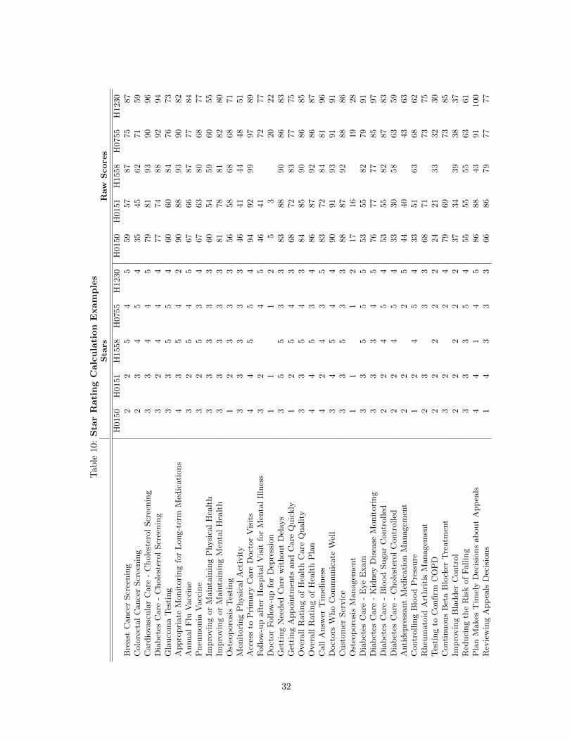
Tables 10 and 11 presents example calculations of the overall summary score and resulting star

values for 5 contracts in 2009. The table lists the summary scores for the individual metrics along

with the corresponding star values, each of which are observed in the raw data. The high mean and

low mean thresholds for i-Factor calculations were calculated to be 3.6667 and 3.2381, respectively.

Similarly, the high variance and low variance thresholds were 1.3462 and 1.0362, respectively.

Table 10 and 11

The calculations for each contract in Table 10 are discussed individually below:

1. Contract H0150: With a mean star value of 2.583 and a variance of 0.879, the contract received

an i-Factor of 0 (due to a low mean), which provided an overall summary score of 2.583 and a

star rating of 2.5.

2. Contract H0151: With a mean star value of 2.667 and a variance of 0.8, the contract received an

i-Factor of 0 (again from a low mean), which provided an overall summary score of 2.667 and a

star rating of 2.5, just 0.083 points away from receiving a 3-star rating.

3. Contract H1558: With a mean star value of 3.967 and a variance of 1.275, the contract received

an i-Factor of 0.3 (high mean and medium variance), which provided an overall summary score

of 4.267, just 0.0167 above the 4.25 threshold required to round up to a 4.5-star rating.

4. Contract H0755: With a mean star value of 3.5278 and a variance of 1.285, the contract re-

ceived an i-Factor of 0.1 (relatively high mean and medium variance), which provided an overall

summary score of 3.6278 and a star rating of 3.5.

5. Contract H1230: With a mean star value of 3.694 and a variance of 1.018, the contract received

an i-Factor of 0.4 (high mean and low variance), which provided an overall summary score of

4.094 and a star rating of 4.0.

22

C Appendix C: Data

Our analysis merges publicly available data from several sources. As our starting point, we merge

together enrollment and contract information by month/year/contract id/plan id for all Medicare

Advantage MA contract/plans from June 2008 through December of 2011.21 For a small number of

counties, CMS reports enrollment counts at the Social Security Administrative (SSA) level.22 For

these observations, we aggregate enrollment to the county level, and, after limiting our focus to

HMO, PPO, and PFFS type contracts, we have a dataset of 50,269,123 observations at the contract

id/plan/county/month/year level.

The enrollment files are invalid for providing a census of MA contracts that operate in a given

market (county) because of migration. For example, if contract A is approved to operate in Orange

County, North Carolina, and an enrollee in contract A moves to Miami-Dade County, Florida, the

enrollment files will report positive enrollment in contract A in Miami-Dade County regardless if

contract A is approved to operate in Miami-Dade. To overcome this problem, CMS provides separate

service area files that list all contracts that are approved to operate in a given county.23 In addition to

the CMS service files, we merge our enrollment dataset to quality star data at the contract/year level24;

CMS contract/plan premium data25; Medicare Advantage market share data at the county/contract

id level26; and county-level census data from the American Community Survey for 2006-2010 in wide

format.

Given the size of the resulting data, we proceed in cleaning the data for 2009 and 2010 separately. In

what follows, we document our cleaning of the 2009 data, with 2010 in parenthesis. Our 2009 (2010)

data contain 19,290,326 (13,427,779) contract id/plan id/county/month observations. We begin by

dropping the 331,272 (204,355) observations from U.S. Territories and Outlying Areas. Next, we drop

all contract/plans that are specific to an employer or union-only group (these are also known as the

“800-series plans”). While the decision to eliminate these plans reduces our sample by 17,051,609

(11,988,547) observations, these contract/plans are not available to the public and are not our primary

21CMS records enrollment data in separate files from contract characteristic information. Data are availableat http://www.cms.gov/Research-Statistics-Data-and-Systems/Statistics-Trends-and-Reports/MCRAdvPartDEnrolData/Monthly-Enrollment-by-

Contract-Plan-State-County.html

22The contract characteristic files contain a small number duplicate observations, which we drop.23Data are available at http://www.cms.gov/Research-Statistics-Data-and-Systems/Statistics-Trends-and-

Reports/MCRAdvPartDEnrolData/MA-Contract-Service-Area-by-State-County.html. For the few counties that are sub-dividedby SSA, we aggregate to the county level.

24Contract-level quality data available at http://www.cms.gov/Medicare/Prescription-Drug-

Coverage/PrescriptionDrugCovGenIn/PerformanceData.html.25Data on plan premiums available at http://www.cms.gov/Medicare/Prescription-Drug-

Coverage/PrescriptionDrugCovGenIn/index.html?redirect=/PrescriptionDrugCovGenIn/. County names and FIPS codes availableat http://www.census.gov/popest/about/geo/codes.html.

26MA penetration data available at http://www.cms.gov/Research-Statistics-Data-and-Systems/Statistics-Trends-and-

Reports/MCRAdvPartDEnrolData/MA-State-County-Penetration.html.

23

focus. Next, we drop the 231,655 (159,439) observations of special needs plans. Finally, we drop the

observations that did not merge perfectly between the CMS enrollment files and the service area files.

These reflect either contracts with positive enrollment in a month/year/county that were not approved

to operate in that county (due to migration) or contracts that were approved to operate in a county

but had no corresponding enrollment record. Our final sample size for 2009 is 1,422,887 (841,790)

contract id/plan id/county/month. We also collect hospital discharge data from the annual Hospital

Cost Reporting Information System (HCRIS) as well as CMS benchmark rates and average FFS costs

by county.27

27Data are available at http://www.cms.gov/Research-Statistics-Data-and-Systems/Files-for-Order/CostReports/Cost-Reports-by-Fiscal-

Year.html.

24

D Appendix D: Additional Analyses

D.1 Robustness Checks

Figure 2 illustrates the sensitivity of the plan-level RD analysis to our bandwidth selection. As should

be the case, the figure closely follows that of the contract-level analysis from Figure 1. Generally, Figure

2 suggests that the findings from the point estimates in Table 4 are relatively persistent across alter-

native bandwidths (provided the bandwidths are sufficiently narrow and include a sufficient number

of contracts).

Figure 2

Figures 4 and 5 present similar graphs for the analysis of plan exit and plan entry, respectively.

The figures generally support the robustness of the point estimates in Tables 6 and 7 to our bandwidth

selection. Our analysis of plan exit and entry at the 2.75 threshold (2.5 versus 3-star contracts) is one

possible exception, with the statistical significance, magnitude, and sign of the point estimates changing

within bandwidths from 0.1 to 0.2. In terms of hypothesis testing, we interpret this as evidence in

favor of the null that the star rating has no effect on plan exit or entry at the 2.75 threshold. As

such, the qualitative findings from our point estimates in Table 6 are unchanged, while the overall

findings from our analysis of plan entry (top panel in in Table 7) are less definitive among 3.0 relative

to 2.5-star rated contracts.

Figures 4 and 5

D.2 Welfare Analysis

The results of estimating equation 6 with OLS and 2SLS are presented in Table 12 along with the

first-stage results for the 2SLS estimator.

25

E Tables and Figures

Table 1: Summary Statistics

2009 2010Mean (S.D.) Mean (S.D.)

Plan-level Data, n=51,442 and 34,642Enrollmenta 291.55 (1,413) 361.17 (1,600)Overall Share % 1.18 1.26Within-nest Share, % 28.87 31.07Premium 37.69 (42.23) 53.27 (52.97)Drug Coverage, % 58.58 64.39HMO, % 16.32 24.12PPO, % 18.53 33.71

Market Characteristics, n=3,139 and 3,094MA Penetration 15.59 (11.03) 16.50 (12.12)Mean Number of Plans 37.38 (22.31) 26.61 (17.58)Population > 65 in 1,000s 12.22 (34.90) 12.59 (35.74)Population > 85 in 1,000s 1.72 (5.11) 1.79 (5.34)Unemployed, % 5.79 9.01White, % 86.30 86.41Black, % 9.11 9.18Female, % 50.16 50.17College Graduates, % 18.68 18.62South, % 42.02 42.63

Contract-level Star Ratings %, n=252 and 2951.5 1.98 0.002.0 9.92 4.072.5 24.21 24.413.0 28.97 29.833.5 21.43 20.674.0 11.11 12.204.5 2.38 7.785.0 0.00 1.02

aEnrollment data available for 20,768 plans in 2009 and 17,334 plans in 2010. Remaining plans have 10 or fewerenrollments and specific enrollments are therefore not provided by CMS.

26

Table 2: OLS Results for Average Characteristicsa

Star Indicator 2.5 3.0 3.5 4.0y = Average Premiumγ2 -5.18*** 6.74*** 6.15*** -8.84***

(1.55) (1.39) (1.54) (2.52)N 4,303 4,182 2,672 1,213R2 0.52 0.66 0.71 0.75y = Proportion of $0 Premium Plansγ2 0.17*** -0.13*** 0.03*** -0.03**

(0.02) (0.01) (0.01) (0.01)N 4,303 4,182 2,672 1,213R2 0.36 0.70 0.75 0.63

aOLS regression of the 2010 mean characteristics on the relevant 2009 mean characteristic and star ratings. Re-gressions estimated separately for each star rating, with γ2 denoting the estimated effect of a one-half star increasein quality ratings. Contract-level averages are based on all plans with more than 10 enrollments. Standard errors inparenthesis are robust to clustering at the county level. Additional controls not in the table include county-level vari-ables on the population over 65, population over 85, unemployment rate, percent white, percent black, percent female,regional dummy (south), percent graduating college, and the number of MA plans and contracts in the county, theCMS benchmark payment rate and average FFS cost, and number of physicians in the county, as well as contract-levelvariables including the number of counties in which the contract operated in 2009, whether the contract operates asan HMO or PPO, and the total number of enrollees under the contract in 2009. * p<0.1. ** p<0.05. *** p<0.01.

Table 3: RD Results for Average Characteristicsa

Star Threshold 2.25 2.75 3.25 3.75y = Average Premiumγ2 4.81 33.60*** 29.30*** 31.85***

(4.27) (7.27) (6.12) (6.38)N 2,029 982 432 309R2 0.39 0.72 0.69 0.92y = Proportion of $0 Premium Plansγ2 -0.14* -0.16** 0.02 -0.13*

(0.08) (0.06) (0.04) (0.07)N 2,029 982 432 309R2 0.21 0.90 0.72 0.55

aResults based on OLS regressions with RD approach and a bandwidth of h = 0.125. Robust standard errors inparenthesis, clustered at the county level. Results were excluded for the 1.5 and 4.5 star ratings due to an insufficientnumber of contracts on the lower and upper ends of the 1.75 and 4.25 thresholds, respectively. Regressions estimatedat the contract level, with dependent variables measured as the average value of each plan characteristic by contract(excluding plans with 10 or fewer enrollments). Additional controls not in the table include county-level variableson the population over 65, population over 85, unemployment rate, percent white, percent black, percent female,regional dummy (south), percent graduating college, and the number of MA plans and contracts in the county, theCMS benchmark payment rate and average FFS cost, and number of physicians in the county, as well as contract-levelvariables including the number of counties in which the contract operated in 2009, whether the contract operates asan HMO or PPO, and the total number of enrollees under the contract in 2009. * p<0.1. ** p<0.05. *** p<0.01.

27

Table 4: RD Results for Plan-level Characteristicsa

Star Threshold 2.25 2.75 3.25 3.75y = 2010 premiumγ2 5.00** 19.40*** 41.99*** 31.52***

(2.10) (3.93) (5.17) (5.10)N 4,912 6,894 1,024 1,082R2 0.63 0.76 0.83 0.94y = Indicator for $0 premium plan in 2010γ2 0.04 -0.32*** 0.02 -0.15***

(0.04) (0.05) (0.03) (0.05)N 4,912 6,894 1,024 1,082R2 0.24 0.89 0.51 0.59

aResults based on OLS regressions with RD approach and a bandwidth of h = 0.125. Robust standard errors inparenthesis, clustered at the county level. Results were excluded for the 1.5 and 4.5 star ratings due to an insufficientnumber of contracts on the lower and upper ends of the 1.75 and 4.25 thresholds, respectively. Regressions estimatedat the plan level for all plans in the dataset. Additional controls not in the table include county-level variables on thepopulation over 65, population over 85, unemployment rate, percent white, percent black, percent female, regionaldummy (south), percent graduating college, and the number of MA plans and contracts in the county, the CMSbenchmark payment rate and average FFS cost, and number of physicians in the county, as well as the plan’s totalnumber of enrollees in 2009 (set to 0 if missing), an indicator variable for missing number of enrollees (¡10 enrolleesin the plan), an indicator for HMO or PPO plan type, and the lagged dependent variable. * p<0.1. ** p<0.05. ***p<0.01.

Table 5: Summary of Plan Exit and Entrya

2009 Rating Exit (%) Entry (%)1.5 Star 99.49 36.512.0 Star 51.40 55.162.5 Star 53.58 52.793.0 Star 29.37 23.913.5 Star 25.97 17.204.0 Star 8.25 32.454.5 Star 8.24 7.72All 49.77 38.20

aExit defined as the same plan-county-contract observation in 2009 no longer active in 2010.

28

Table 6: RD Results for Plan Exita

Star Threshold 2.25 2.75 3.25 3.75Overall Resultsγ2 -0.83*** -0.07 0.12** -0.25***

(0.06) (0.09) (0.06) (0.06)N 10,791 9,806 1,177 1,435Among Plans with Premiums = $0γ2 -0.84*** 0.25** 1.07*** -0.07

(0.06) (0.11) (0.30) (0.05)N 9,110 613 140 281Among Plans with Premiums > $0γ2 -1.37*** -0.82*** 0.04 -0.36***

(0.13) (0.12) (0.05) (0.07)N 1,681 9,193 1,037 1,154

aResults based on linear probability model with RD approach and a bandwidth of h = 0.125. Robust standarderrors in parenthesis, clustered at the county level. Results were excluded for the 1.5 and 4.5 star ratings due to aninsufficient number of contracts on the lower and upper ends of the 1.75 and 4.25 thresholds, respectively. Additionalcontrols not in the table include county-level variables on the population over 65, population over 85, unemploymentrate, percent white, percent black, percent female, regional dummy (south), percent graduating college, and thenumber of MA plans and contracts in the county, the CMS benchmark payment rate and average FFS cost, andnumber of physicians in the county, as well as 2009 plan characteristics and enrollment. * p<0.1. ** p<0.05. ***p<0.01.

Table 7: RD Results for Plan Entrya

Star Threshold 2.25 2.75 3.25 3.75Overall Resultsγ2 0.06 -0.23*** 0.18*** 0.30***

(0.12) (0.07) (0.06) (0.06)N 6,352 2,453 1,252 852Among Plans with Premiums = $0γ2 -0.76*** -0.02 -1.80** 0.65***

(0.08) (0.09) (0.75) (0.12)N 3,360 793 171 331Among Plans with Premiums > $0γ2 2.34*** -1.28*** 0.22*** 0.20***

(0.16) (0.19) (0.07) (0.06)N 2,992 1,660 1,081 521

aResults based on linear probability model with RD approach and a bandwidth of h = 0.125. Robust standarderrors in parenthesis, clustered at the county level. Results were excluded for the 1.5 and 4.5 star ratings due to aninsufficient number of contracts on the lower and upper ends of the 1.75 and 4.25 thresholds, respectively. Additionalcontrols not in the table include county-level variables on the population over 65, population over 85, unemploymentrate, percent white, percent black, percent female, regional dummy (south), percent graduating college, the CMSbenchmark payment rate and average FFS cost, and number of physicians in the county, as well as plan characteristics(premium, Part D participation, and HMO versus PPO). * p<0.1. ** p<0.05. *** p<0.01.

29

Table 8: RD Results for Premiums without Covariatesa

Star Threshold 2.25 2.75 3.25 3.75y = Mean Contract Premiumsγ2 12.82 16.25*** 28.58*** 26.97***

(3.26) (4.53) (5.09) (12.66)N 2,029 982 432 309y = Individual Plan Premiumsγ2 -4.34*** 10.88*** 31.27*** 8.36

(1.59) (2.31) (3.42) (7.23)N 4,912 6,894 1,024 1,082

aResults based on RD with triangular kernel and a bandwidth of h = 0.125. Results were excluded for the 1.5 and4.5 star ratings due to an insufficient number of contracts on the lower and upper ends of the 1.75 and 4.25 thresholds,respectively. * p<0.1. ** p<0.05. *** p<0.01.

30

Tab

le9:

Domains,

Metrics,

and

Data

Sourcesfor2009M

ASta

rRatingPro

gra

ma

Sta

yingHealthy

GettingTim

ely

Care

from

Docto

rsPlan

Resp

onsiveness

and

Care

ManagingChro

nic

Conditions

HandlingofAppeals

Bre

ast

Cance

rScr

eenin

g(H

ED

IS)

Acc

ess

toP

rim

ary

Care

Doct

or

Vis

its

(HE

DIS

)G

etti

ng

App

oin

tmen

tsand

Care

Quic

kly

(CA

HP

S)

Ost

eop

oro

sis

Managem

ent

(HE

DIS

)P

lan

Makes

Tim

ely

Dec

isio

ns

ab

out

App

eals

(IR

E)

Colo

rect

al

Cance

rScr

eenin

g(H

ED

IS)

Follow

-up

Vis

itw

ithin

30

Day

sof

Dis

charg

eaft

erH

osp

ital

Sta

yfo

rM

enta

lIl

lnes

s(H

ED

IS)

Over

all

Rati

ng

of

Hea

lth

Care

Quality

(CA

HP

S)

Dia

bet

esC

are

-E

ye

Exam

(HE

DIS

)R

evie

win

gA

pp

eals

Dec

isio

ns

(IR

E)

Card

iova

scula

rC

are

-C

hole

ster

ol

Scr

eenin

g(H

ED

IS)

Doct

or

Follow

-up

for

Dep

ress

ion

(HE

DIS

)O

ver

all

Rati

ng

of

Hea

lth

Pla

n(C

AH

PS)

Dia

bet

esC

are

-K

idney

Dis

ease

Monit

ori

ng

(HE

DIS

)

Dia

bet

esC

are

-C

hole

ster

ol

Scr

eenin

g(H

ED

IS)

Get

ting

Nee

ded

Care

wit

hout

Del

ays

(CA

HP

S)

Call

Answ

erT

imel

ines

s(H

ED

IS)

Dia

bet

esC

are

-B

lood

Sugar

Contr

olled

(HE

DIS

)

Gla

uco

ma

Tes

ting

(HE

DIS

)D

oct

ors

Who

Com

munic

ate

Wel

l(C

AH

PS)

Dia

bet

esC

are

-C

hole

ster

ol

Contr

olled

(HE

DIS

)

Appro

pri

ate

Monit

ori

ng

of

Pati

ents

Takin

gL

ong-T

erm

Med

icati

ons

(HE

DIS

)

Cust

om

erSer

vic

e(C

AH

PS)

Anti

dep

ress

ant

Med

icati

on

Managem

ent

(HE

DIS

)

Annual

Flu

Vacc

ine

(CA

HP

S)

Contr

ollin

gB

lood

Pre

ssure

(HE

DIS

)

Pneu

monia

Vacc

ine

(CA

HP

S)

Rheu

mato

idA

rthri

tis

Managem

ent

(HE

DIS

)

Impro

vin

gor

Main

tain

ing

Physi

cal

Hea

lth

(HO

S)

Tes

ting

toC

onfirm

CO

PD

(HE

DIS

)

Impro

vin

gor

Main

tain

ing

Men

tal

Hea

lth

(HO

S)

Conti

nuous

Bet

aB

lock

erT

reatm

ent

(HE

DIS

)

Ost

eop

oro

sis

Tes

ting

(HO

S)

Impro

vin

gB

ladder

Contr

ol

(HO

S)

Monit

ori

ng

Physi

cal

Act

ivit

y(H

OS)

Red

uci

ng

the

Ris

kof

Fallin

g(H

OS)

aD

escr

ipti

on

of

dom

ain

san

dad

dit

ional

det

ails

availab

leat

ww

w.c

ms.

gov.

Data

sou

rce

for

CM

Sca

lcu

lati

on

sp

rovid

edin

pare

nth

esis

.

31

Tab

le10:Sta

rRatingCalculation

Examples

Sta

rsRaw

Score

s

H0150

H0151

H1558

H0755

H1230

H0150

H0151

H1558

H0755

H1230

Bre

ast

Cance

rScr

eenin

g2

25

45

59

57

87

75

87

Colo

rect

al

Cance

rScr

eenin

g2

34

54

35

45

62

71

59

Card

iova

scula

rC

are

-C

hole

ster

ol

Scr

eenin

g3

34

45

79

81

93

90

96

Dia

bet

esC

are

-C

hole

ster

ol

Scr

eenin

g3

24

44

77

74

88

92

94

Gla

uco

ma

Tes

ting

33

55

460

60

84

76

73

Appro

pri

ate

Monit

ori

ng

for

Long-t

erm

Med

icati

ons

43

54

290

88

93

90

82

Annual

Flu

Vacc

ine

32

54

567

66

87

77

84

Pneu

monia

Vacc

ine

32

53

467

63

80

68

77

Impro

vin

gor

Main

tain

ing

Physi

cal

Hea

lth

33

33

360

54

59

60

55

Impro

vin

gor

Main

tain

ing

Men

tal

Hea

lth

33

33

381

78

81

82

80

Ost

eop

oro

sis

Tes

ting

12

33

356

58

68

68

71

Monit

ori

ng

Physi

cal

Act

ivit

y3

33

33

46

41

44

48

51

Acc

ess

toP

rim

ary

Care

Doct

or

Vis

its

44

55

494

92

99

97

89

Follow

-up

aft

erH

osp

ital

Vis

itfo

rM

enta

lIl

lnes

s3

24

546

41

72

77

Doct

or

Follow

-up

for

Dep

ress

ion

11

12

53

20

22

Get

ting

Nee

ded

Care

wit

hout

Del

ays

35

53

383

88

90

86

83

Get

ting

App

oin

tmen

tsand

Care

Quic

kly

12

54

368

72

83

77

75

Over

all

Rati

ng

of

Hea

lth

Care

Quality

33

54

384

85

90

86

85

Over

all

Rati

ng

of

Hea

lth

Pla

n4

45

34

86

87

92

86

87

Call

Answ

erT

imel

ines

s4

24

35

83

72

84

81

96

Doct

ors

Who

Com

munic

ate

Wel

l3

45

44

90

91

93

91

91

Cust

om

erSer

vic

e3

35

33

88

87

92

88

86

Ost

eop

oro

sis

Managem

ent

11

12

17

16

19

28

Dia

bet

esC

are

-E

ye

Exam

33

55

553

55

82

79

91

Dia

bet

esC

are

-K

idney

Dis

ease

Monit

ori

ng

33

34

576

77

77

85

97

Dia

bet

esC

are

-B

lood

Sugar

Contr

olled

22

45

453

55

82

87

83

Dia

bet

esC

are

-C

hole

ster

ol

Contr

olled

22

45

433

30

58

63

59

Anti

dep

ress

ant

Med

icati

on

Managem

ent

22

25

44

40

43

63

Contr

ollin

gB

lood

Pre

ssure

12

45

433

51

63

68

62

Rheu

mato

idA

rthri

tis

Managem

ent

23

33

68

71

73

75

Tes

ting

toC

onfirm

CO

PD

22

22

224

21

33

32

30

Conti

nuous

Bet

aB

lock

erT

reatm

ent

32

24

79

69

73

85

Impro

vin

gB

ladder

Contr

ol

22

22

237

34

39

38

37

Red

uci

ng

the

Ris

kof

Fallin

g3

33

54

55

55

55

63

61

Pla

nM

akes

Tim

ely

Dec

isio

ns

ab

out

App

eals

44

14

586

88

43

91

100

Rev

iew

ing

App

eals

Dec

isio

ns

14

33

366

86

79

77

77

32

Table 11: Star Rating Calculation Examples, Cont.H0150 H0151 H1558 H0755 H1230

Mean Summary Score 2.5833 2.6667 3.9667 3.5278 3.6944Variance Summary Score 0.8786 0.80 1.2747 1.2849 1.0183i-Factor 0 0 0.3 0.1 0.4Summary Score 2.5833 2.6667 4.2667 3.6278 4.0944Star Rating 2.5 2.5 4.5 3.5 4

Table 12: Welfare Analysisa

OLS 2SLS

Premium -0.00** -0.04***(0.00) (0.01)

Within-group Share 0.71*** 0.74***(0.03) (0.10)

HMO -0.03 -1.26**(0.09) (0.61)

PPO -0.21 -0.55(0.13) (0.38)

Part D 1.19*** 2.22***(0.11) (0.48)

Part D Cost -0.00 -0.00(0.00) (0.00)

Summary Score 0.43*** 1.96***(0.10) (0.63)

N 20,738 18,300First-stage Statistics

Premium Within-group Share

Contract Count 0.07 -0.00(0.30) (0.01)

Hospital Inpatient HHI -0.27 1.45***(1.31) (0.04)

Hospital Count -0.43*** -0.00(0.10) (0.00)

Total Physicians 0.00 -0.00***(0.00) (0.00)

F-stat 9.80 647.94

aRobust standard errors in parenthesis, clustered at the contract level. In the 2SLS estimation, premium andwithin group share were instrumented using number of contracts operating in a county, the number of hospitals ina county, the Herfindahl-Hirschman Index (HHI) for hospitals in a county (based on discharges), and the number ofphysicians in the county as instruments. * p<0.1. ** p<0.05. *** p<0.01.

33

Figure 1: Effect of Star Rating on Mean Contract Premium for Varying Bandwidths Around Thresholds2.25, 2.75, 3.25 and 3.75

-40

-20

020

Sta

r R

atin

g C

oeffi

cien

t, g 2

.1 .15 .2 .25

Bandwidth

1020

3040

5060

Sta

r R

atin

g C

oeffi

cien

t, g 2

.1 .15 .2 .25

Bandwidth

a. 2.25 b. 2.75

1020

3040

50

Sta

r R

atin

g C

oeffi

cien

t, g 2

.1 .15 .2 .25

Bandwidth

-20

020

4060

Sta

r R

atin

g C

oeffi

cien

t, g 2

.1 .15 .2 .25

Bandwidth

c. 3.25 d. 3.75

34

Figure 2: Effect of Star Rating on Plan Premiums for Varying Bandwidths Around Thresholds 2.25,2.75, 3.25 and 3.75

-10

-50

510

15

Sta

r R

atin

g C

oeffi

cien

t, g 2

.1 .2 .3 .4 .5

Bandwidth

010

2030

40

Sta

r R

atin

g C

oeffi

cien

t, g 2

.1 .2 .3 .4 .5

Bandwidth

a. 2.25 b. 2.75

3040

5060

7080

Sta

r R

atin

g C

oeffi

cien

t, g 2

.1 .2 .3 .4 .5

Bandwidth

020

4060

Sta

r R

atin

g C

oeffi

cien

t, g 2

.1 .2 .3 .4 .5

Bandwidth

c. 3.25 d. 3.75

35

Figure 3: Falsification Test: Effect of Star Rating on Mean Contract Premium around Counter-factualThresholds

-50

050

100

Sta

r R

atin

g C

oeffi

cien

t, g 2

2.1 2.2 2.3 2.4

Counterfactual Threshold

-40

-20

020

4060

Sta

r R

atin

g C

oeffi

cien

t, g 2

2.6 2.7 2.8 2.9

Counterfactual Threshold

a. Around the true 2.25 threshold b. Around the true 2.75 threshold

-100

-50

050

100

Sta

r R

atin

g C

oeffi

cien

t, g 2

3.1 3.2 3.3 3.4

Counterfactual Threshold

-50

050

Sta

r R

atin

g C

oeffi

cien

t, g 2

3.6 3.7 3.8 3.9

Counterfactual Threshold

c. Around the true 3.25 threshold d. Around the true 3.75 threshold

36

Figure 4: Effect of Star Rating on Plan Exit for Varying Bandwidths Around Thresholds 2.25, 2.75,3.25 and 3.75

-1.5

-1-.

50

Sta

r R

atin

g C

oeffi

cien

t, g 2

.1 .2 .3 .4 .5

Bandwidth

-1.5

-1-.

50

.5

Sta

r R

atin

g C

oeffi

cien

t, g 2

.1 .2 .3 .4 .5

Bandwidth

a. 2.25 b. 2.75

-.4

-.2

0.2

.4

Sta

r R

atin

g C

oeffi

cien

t, g 2

.1 .2 .3 .4 .5

Bandwidth

-.6

-.4

-.2

0

Sta

r R

atin

g C

oeffi

cien

t, g 2

.1 .2 .3 .4 .5

Bandwidth

c. 3.25 d. 3.75

37

Figure 5: Effect of Star Rating on Plan Entry for Varying Bandwidths Around Thresholds 2.25, 2.75,3.25 and 3.75

-10

12

Sta

r R

atin

g C

oeffi

cien

t, g 2

.1 .2 .3 .4 .5

Bandwidth

-.6

-.4

-.2

0.2

.4

Sta

r R

atin

g C

oeffi

cien

t, g 2

.1 .2 .3 .4 .5

Bandwidth

a. 2.25 b. 2.75

-.1

0.1

.2.3

.4

Sta

r R

atin

g C

oeffi

cien

t, g 2

.1 .2 .3 .4 .5

Bandwidth

0.1

.2.3

.4.5

Sta

r R

atin

g C

oeffi

cien

t, g 2

.1 .2 .3 .4 .5

Bandwidth

c. 3.25 d. 3.75

38