Page 1
QUANTIFICATION OF THERMOELECTRIC ENERGY
SCAVENGING OPPORTUNITY IN NOTEBOOK COMPUTERS
A THESIS SUBMITTED TO
THE BOARD OF CAMPUS GRADUATE PROGRAMS OF
MIDDLE EAST TECHNICAL UNIVERSITY,
NORTHERN CYPRUS CAMPUS
BY
REHA DENKER
IN PARTIAL FULLFILLMENT OF THE REQUIREMENTS
FOR
THE DEGREE OF MASTER OF SCIENCE
IN
SUSTAINABLE ENVIRONMENT AND ENERGY SYSTEMS
AUGUST 2012
Page 2
Approval of the thesis:
QUANTIFICATION OF THERMOELECTRIC ENERGY SCAVENGING
OPPORTUNITY IN NOTEBOOK COMPUTERS
submitted by REHA DENKER in partial fulfillment of the requirements for the degree of
Master of Science in Sustainable Environment and Energy Systems (SEES) program,
Middle East Technical University, Northern Cyprus Campus (METU-NCC) by,
Prof. Dr. Erol Taymaz
Chair of the Board of Graduate Programs
Asst. Prof. Dr. Ali Muhtaroğlu
Program Coordinator, SEES Program
Asst. Prof. Dr. Ali Muhtaroğlu
Supervisor, Electrical Engineering Dept.
Examining Committee Members:
Asst. Prof. Dr. Eray Uzgören
Mechanical Engineering Dept., METU-NCC
Asst. Prof. Dr. Ali Muhtaroğlu
Electrical Engineering Dept., METU-NCC
Assoc. Prof. Dr. Haluk Külah
Electrical Engineering Dept., METU
Inst. Dr. Murat Sönmez
Mechanical Engineering Dept., METU-NCC
Asst. Prof. Dr. Volkan Esat
Mechanical Engineering Dept., METU-NCC
Date: August 16th, 2012
Page 3
iii
I hereby declare that all information in this document has been obtained and
presented in accordance with academic rules and ethical conduct. I also declare that,
as required by these rules and conduct, I have fully cited and referenced all material
and results that are not original to this work.
Name, Last name :
Signature :
Page 4
iv
ABSTRACT
QUANTIFICATION OF THERMOELECTRIC ENERGY SCAVENGING
OPPORTUNITY IN NOTEBOOK COMPUTERS
Denker, Reha
M.S., Sustainable Environment and Energy Program
Supervisor: Asst. Prof. Dr. Ali Muhtaroğlu
Co-Supervisor: Assoc. Prof. Dr. Haluk Külah
August 2012, 104 pages
Thermoelectric (TE) module integration into a notebook computer is experimentally
investigated in this thesis for its energy harvesting opportunities. A detailed Finite
Element (FE) model was constructed first for thermal simulations. The model outputs
were then correlated with the thermal validation results of the selected system. In parallel,
a commercial TE micro-module was experimentally characterized to quantify maximum
power generation opportunity from the combined system and component data set. Next,
suitable “warm spots” were identified within the mobile computer to extract TE power
with minimum or no notable impact to system performance, as measured by thermal
changes in the system, in order to avoid unacceptable performance degradation. The
prediction was validated by integrating a TE micro-module to the mobile system under
test. Measured TE power generation power density in the carefully selected region of the
heat pipe was around 1.26 mW/cm3 with high CPU load. The generated power scales
down with lower CPU activity and scales up in proportion to the utilized opportunistic
space within the system. The technical feasibility of TE energy harvesting in mobile
computers was hence experimentally shown for the first time in this thesis.
Keywords: Thermoelectric Energy Harvesting, Thermoelectric Power Generation, Mobile
Computers, Sustainable Energy
Page 5
v
ÖZ
DİZÜSTÜ BİLGİSAYARLARDA TERMOELEKTRİK ENERJİ ÜRETİM
OLANAĞININ SAYISAL OLARAK İNCELENMESİ
Denker, Reha
Yüksek Lisans, Sürdürülebilir Çevre ve Enerji Sistemleri Programı
Tez Yöneticisi: Yrd. Doç. Dr. Ali Muhtaroğlu
Ortak Tez Yöneticisi: Doç. Dr. Haluk Külah
Ağustos 2012, 104 sayfa
Bu çalışmada, dizüstü bir bilgisayara eklenen termoelektrik kapsül vasıtasıyla enerji
üretimi fırsatları deneysel olarak incelenmiştir. Isıl simulasyonlar için detaylı bir sonlu
analiz modeli hazırlanmıştır. Bu modelden elde edilen sonuçlar daha sonra test
sisteminden toplanan bulgularla bağdaştırılmıştır. Aynı zamanda ticari bir termoelektrik
mikro kapsülü deneysel olarak karakterize edilmiş ve bu kapsül ile sistemin hangi
koşullarda azami güç üretimi için elverişli olacağı sayısal olarak analiz edilmiştir.
Akabinde, dizüstü bilgisayar içerisinde thermoelektrik kapsül için uygun olabilecek “sıcak
noktalar” belirlenmiştir. Bu noktaların belirlenmesi esnasında ısıl ölçümler sürekli göz
önünde tutulmuş ve sistemin aşırı ısınmasına veya performans kaybına sebep olmayacak
noktaların seçilmesi özellikle dikkate alınmıştır. Önceki aşamalarda yapılan tahminlerin
doğrulanması için çalışır durumdaki test sistemine termoelektrik kapsüller eklenmiştir.
Mikroişlemci yüksek iş yüküyle çalışırken, ısı boruları civarındaki termoelektrik güç
üretim yoğunluğu 1.26 mW/cm3 olarak ölçülmüştür. Üretilen güç miktarı, mikroişlemci
faaliyeti ve kullanılan ısıl alan miktarı ile orantılı miktarda hareket etmektedir. Dizüstü
bilgisayarlarda termoelektrik enerji üretimi uygulanabilirliği bu tezde gösterilmiştir.
Anahtar Kelimeler: Termoelektrik Enerji Geri Kazanımı, Termoelektrik Güç Üretimi,
Dizüstü Bilgisayarlar, Sürdürülebilir Enerji
Page 6
vi
DEDICATION
I would like to dedicate this work to my mother, my father, my sister, Yağız and Ayşim;
for their unconditional support and trust during my whole research and thesis writing
process.
Page 7
vii
ACKNOWLEDGEMENTS
The author wishes to express his deepest gratitude to his advisor Assistant Professor Dr.
Ali Muhtaroğlu for his guidance, advice, criticism, encouragements and insight
throughout the research.
The author would like to thank Associate Professor Dr. Haluk Külah from Middle East
Technical University MEMS Research Center, Mr. Rajiv Mongia from Intel and Assistant
Professor Dr. Eray Uzgören from Middle East Technical University Northern Cyprus
Campus for their contributions in reviewing different parts of this work, and to Hamburg
Industries Co. Ltd. for donating a replacement for a damaged cable in the target system.
The technical assistance of Mr. Saim Seloğlu and Mr. İzzet Akmen are gratefully
acknowledged.
This work is in part supported by MER, a partnership of the Intel Corporation to conduct
and promote research in the Middle East and in part by TÜBİTAK, Turkey under grant
number 109E220.
Page 8
viii
TABLE OF CONTENTS
ABSTRACT………………………………………………………………………..... iv
ÖZ………………………………………………………………………………….... v
DEDICATION………………………………………………………………………. vi
ACKNOWLEDGEMENTS…………………………………………………………. vii
TABLE OF CONTENTS……………………………………………………………. viii
LIST OF FIGURES…………………………………………………………………. x
LIST OF TABLES…………………………………………………………………... xiii
NOMENCLATURE………………………………………………………………… xv
CHAPTER
1. INTRODUCTION…………………………………………………………….. 1
1.1 Energy Harvesting…………………………………………………….... 1
1.2 Thesis Objective………………………………………………………… 3
2. BACKGROUND AND PREVIOUS WORK…………………………………. 5
2.1 Background Research…………………………………………………... 5
2.1.1 Thermoelectric Modules…………………………………………... 5
2.1.2 Applications in Microelectronic Systems…………………………. 9
2.2 Previous Work………………………………………………………….. 12
3. CHARACTERIZATION OF THERMOELECTRIC MODULES…………… 15
4. MECHANICAL AND THERMAL CHARACTERIZATION OF THE
PLATFORMS…………………………………………………………………….
22
4.1 Selection and Basic Specifications of the Test Systems………………... 22
4.2 Characterization of the First Test System: Toshiba Portégé R705-P25... 25
4.3 Characterization of the Second Test System: Dell Alienware M17xR2... 32
4.4 Selection of the Target System…………………………………………. 40
Page 9
ix
4.5 Effects of the TE Module Integration on the Carbon Footprint……...…. 40
5. TARGET SYSTEM MODELING……………………………………………. 42
6. THERMOELECTRIC MODULE INTEGRATION ANALYSIS AND
VALIDATION…………………………………………………………………...
48
6.1 Selecting a Feasible Integration Point for TE Module………………...... 48
6.2 TE Module Integration and Analysis…………………………………… 52
6.3 Full Simulation with TE Module……………………………………….. 57
6.4 Verification of the Results……………………………………………… 58
7. CONCLUSION……………………………………………………………….. 63
7.1 Thesis Conclusion………………………………………………………. 63
7.2 Future Work…………………………………………………………….. 64
REFERENCES……………………………………………………………………… 65
APPENDICES
A. DATASHEETS OF TE CHARACTERIZATION EXPERIMENT………….. 68
B. DATA COLLECTED FROM TOSHIBA PORTÉGÉ R705-P25……………. 73
C. DATA COLLECTED FROM DELL ALIENWARE M17XR2……………… 76
D. INTEGRATED TE MODULE MEASUREMENTS………………………… 80
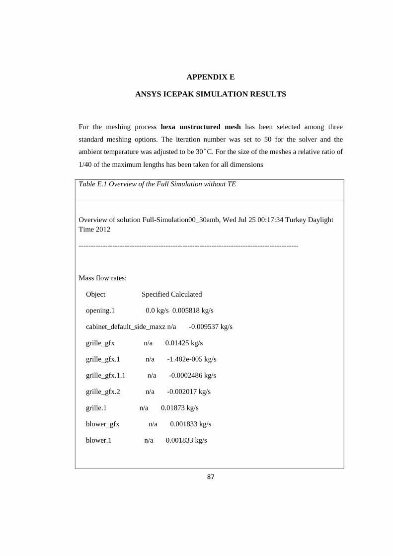
E. ANSYS ICEPAK SIMULATION……………………………………………. 87
Page 10
x
LIST OF FIGURES
Figure 1.1 Relative improvements in notebook computing technology between
1990 –2003. Note the wireless connectivity curve considers only cellular
standards; not short-range 802.11 “hotspots”…………………………………….
1
Figure 1.2 Steps in experimental development of TE generation in notebook
systems…
4
Figure 2.1 Thermoelectric couple in (a) cooler, and (b) generator configuration…... 6
Figure 2.2 Schematics of a thermoelectric generator……………………………….. 6
Figure 2.3 Potential barrier Vh(xh) profile between electrodes with different
temperatures and electrode work functions. The solid line is the real potential
profile taking into account the image charge correction, the dotted one is the
trapezoidal approximation without correction…………………………………....
8
Figure 2.4 The Seiko Thermic wristwatch: (a) the product; (b) a cross-sectional
diagram; (c) thermoelectric modules; (d) a thermopile array. Copyright by Seiko
Instruments……………………………………………………………………….
9
Figure 2.5 Cross-section of the thin film rechargeable battery……………………… 10
Figure 2.6 The schematics of a) direct attach, b) shunt attach………………………. 11
Figure 2.7 Mobile platform a) average power usage, and b) thermal design power... 13
Figure 2.8 Illustration of the TE energy harvesting model, created by Rocha et al... 14
Figure 3.1 TE model characterization setup prepared for this thesis………………... 15
Figure 3.2 Schematics of TE module characterization setup………………………... 16
Figure 3.3 Thevenin circuit built for electrical data acquisition…………………….. 18
Figure 3.4 The Seebeck coefficients (mV/ °C) versus the temperature difference
(Kelvin or degree Celsius) across the selected TE modules……………………...
20
Figure 3.5 Measured open circuit voltage values (mV) versus the temperature
difference (Kelvin or degree Celsius) across the selected TE modules…………..
20
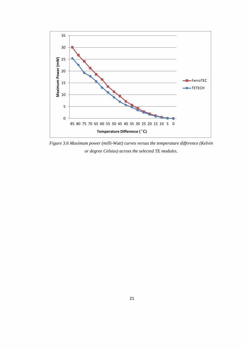
Figure 3.6 Maximum power (milli-Watt) curves versus the temperature difference
(Kelvin or degree Celsius) across the selected TE modules……………………...
21
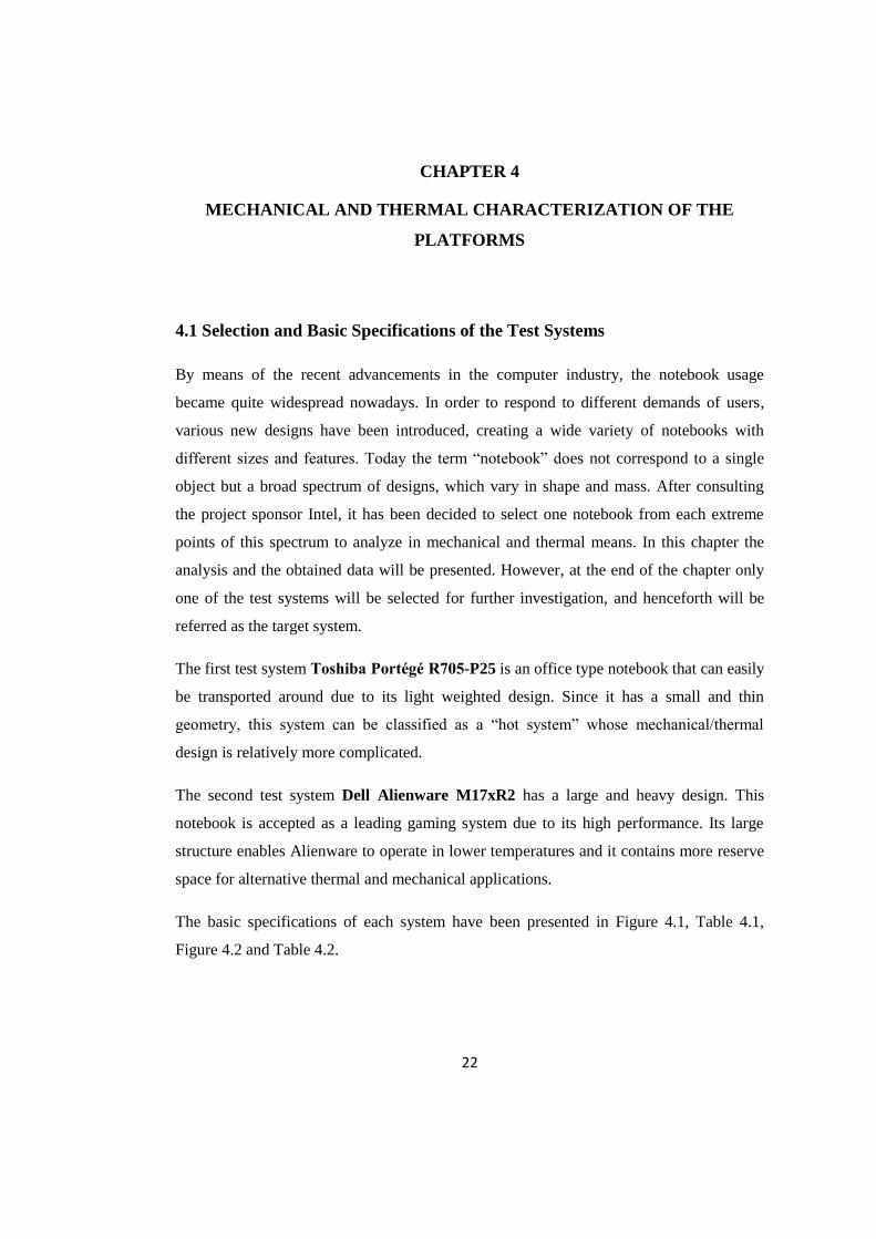
Figure 4.1 Toshiba Portégé R705-P25 office type notebook………………………... 23
Page 11
xi
Figure 4.2 Dell Alienware M17xR2 model high performance notebook…………… 24
Figure 4.3 Toshiba internal schematics……………………………………………... 25
Figure 4.4 Toshiba temperature measurements………………………....................... 25
Figure 4.5 Thermal Analysis Tools (TAT) Screenshot……………………………... 26
Figure 4.6 Toshiba external measurement points (top layer)……………………….. 27
Figure 4.7 Toshiba external measurement points (bottom layer)…………………… 27
Figure 4.8 Selected measurement data from the chassis of Toshiba (under 80%
workload)…………………………………………………………………………
28
Figure 4.9 Selected measurement data from the chassis of Toshiba (under 100%
workload)…………………………………………………………………………
28
Figure 4.10 Toshiba internal photo (with thermocouples connected)……………… 29
Figure 4.11 Toshiba internal data (T1-T5) and data acquired from TAT under 80%
workload………………………………………………………………………….
30
Figure 4.12. Alienware mechanical schematics (first layer)………………………... 32
Figure 4.13 Alienware mechanical schematics (second layer) and the thermal
measurement points………………………………………………………………
33
Figure 4.14 Alienware, photo of the second layer (graphics card removed)………... 33
Figure 4.15 Alienware third layer (with the thermal shield)……………………….. 34
Figure 4.16 Alienware thermal photos ((a) with high contrast, (b) with normal
contrast)…………………………………………………………………………..
34
Figure 4.17 Thermal photo overlaid on the mechanical map……………………….. 35
Figure 4.18 Measurement points on the notebook chassis………………………….. 36
Figure 4.19 Temperature measurements of the selected points inside the test system
while operating with 80% CPU workload………………………………………..
37
Figure 4.20 Temperature measurements of the selected points inside the test system
while operating with 100% CPU workload………………………………………
38
Figure 5.1 Motherboard of the target system………………………………………... 42
Figure 5.2 A screenshot representing the results of the CPU simulation…………… 43
Figure 5.3 Utilized mesh control settings of Icepak………………………………… 44
Figure 5.4 ATI Mobility Radeon HD 5870 model graphics card…………………… 45
Figure 5.5 A screenshot from the simulation of GFX………………………………. 46
Page 12
xii
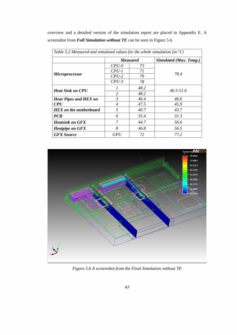
Figure 5.6 A screenshot from the Final Simulation without TE…………………….. 47
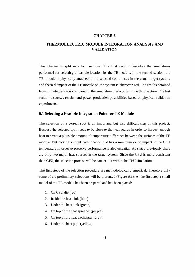
Figure 6.1 The locations of the preliminarily selected points for TE module………. 49
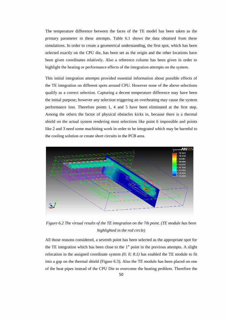
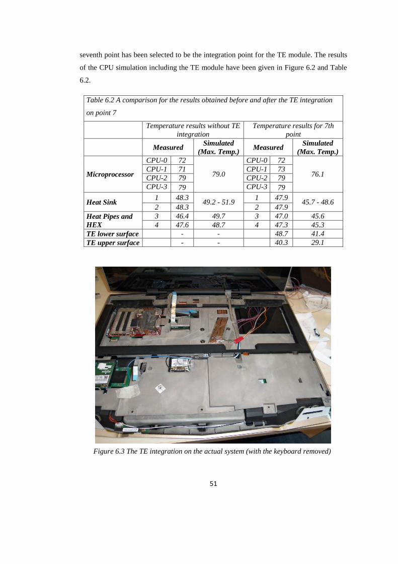
Figure 6.2 The virtual results of the TE integration on the 7th point……………….. 50
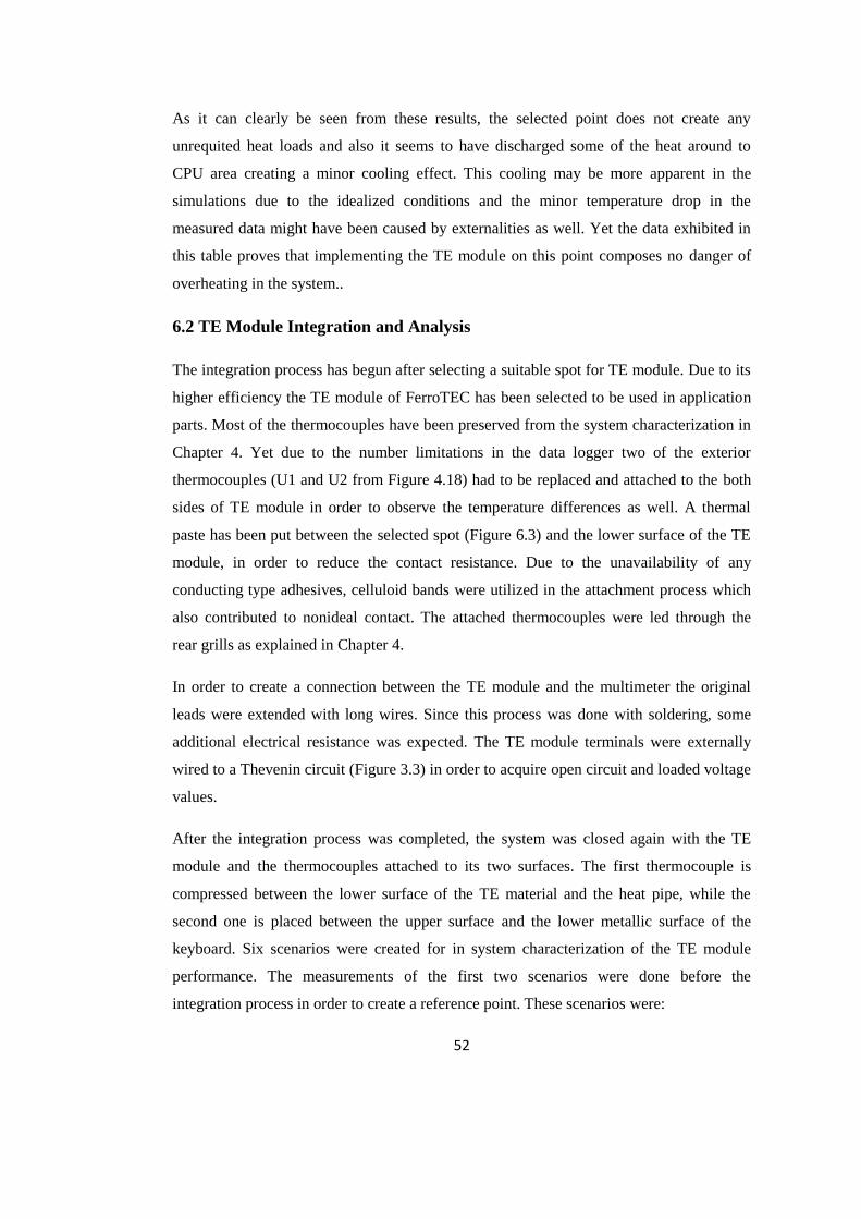
Figure 6.3 The TE integration on the actual system (with the keyboard removed).... 51
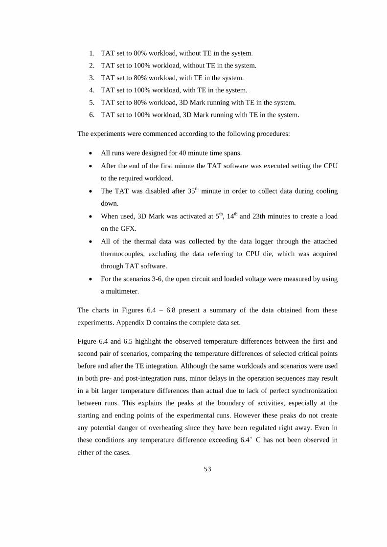
Figure 6.4 Temperature differences between the pre- and post TE integration cases
for some selected points when CPU operates in 80% workload…………………
54
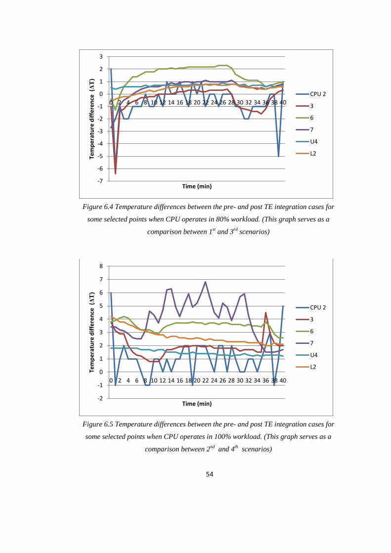
Figure 6.5 Temperature differences between the pre- and post TE integration cases
for some selected points when CPU operates in 100% workload………………..
54
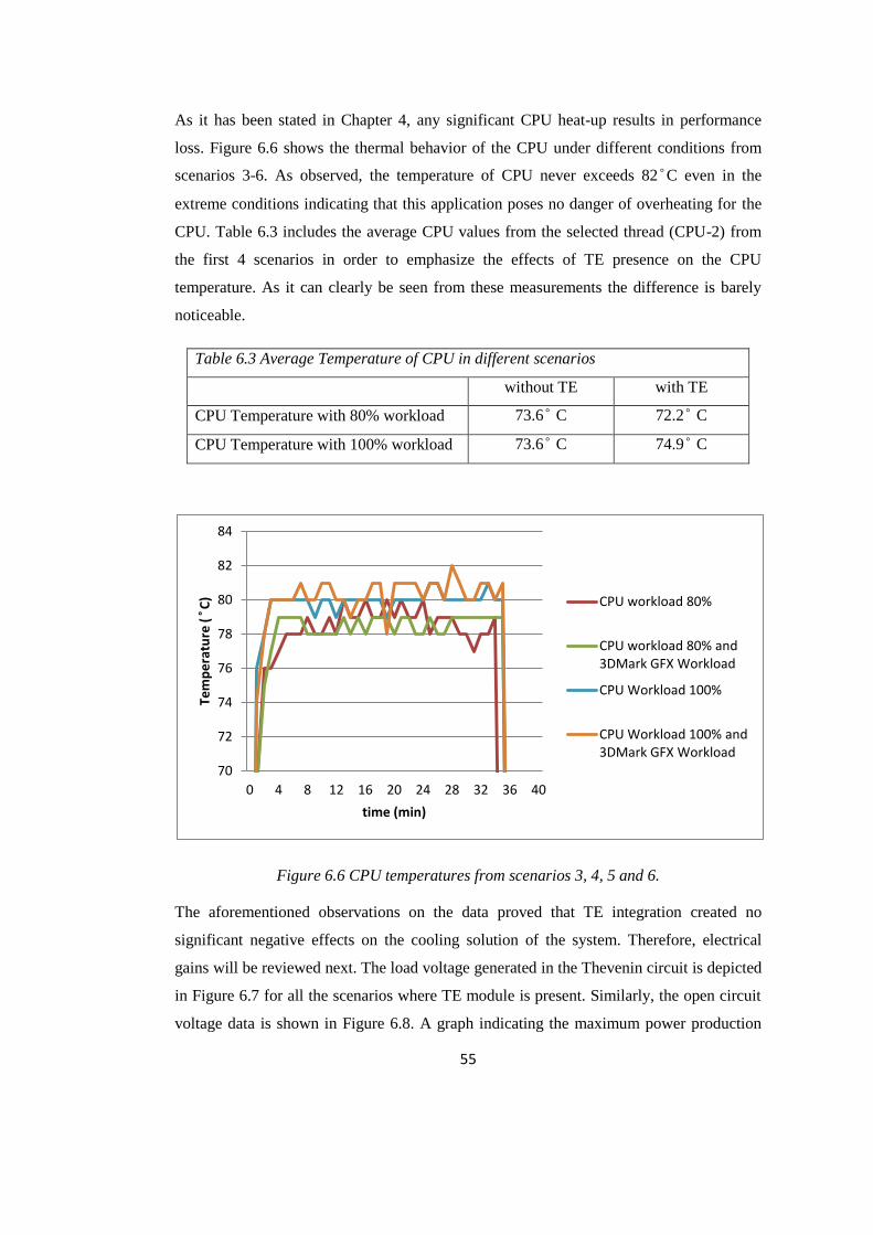
Figure 6.6 CPU temperatures from scenarios 3, 4, 5 and 6…………………………. 55
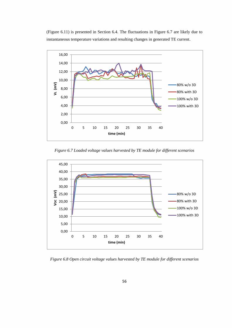
Figure 6.7 Loaded voltage values harvested by TE module for different scenarios... 56
Figure 6.8 Open circuit voltage values harvested by TE module for different
scenarios………………………………………………………………………….
56
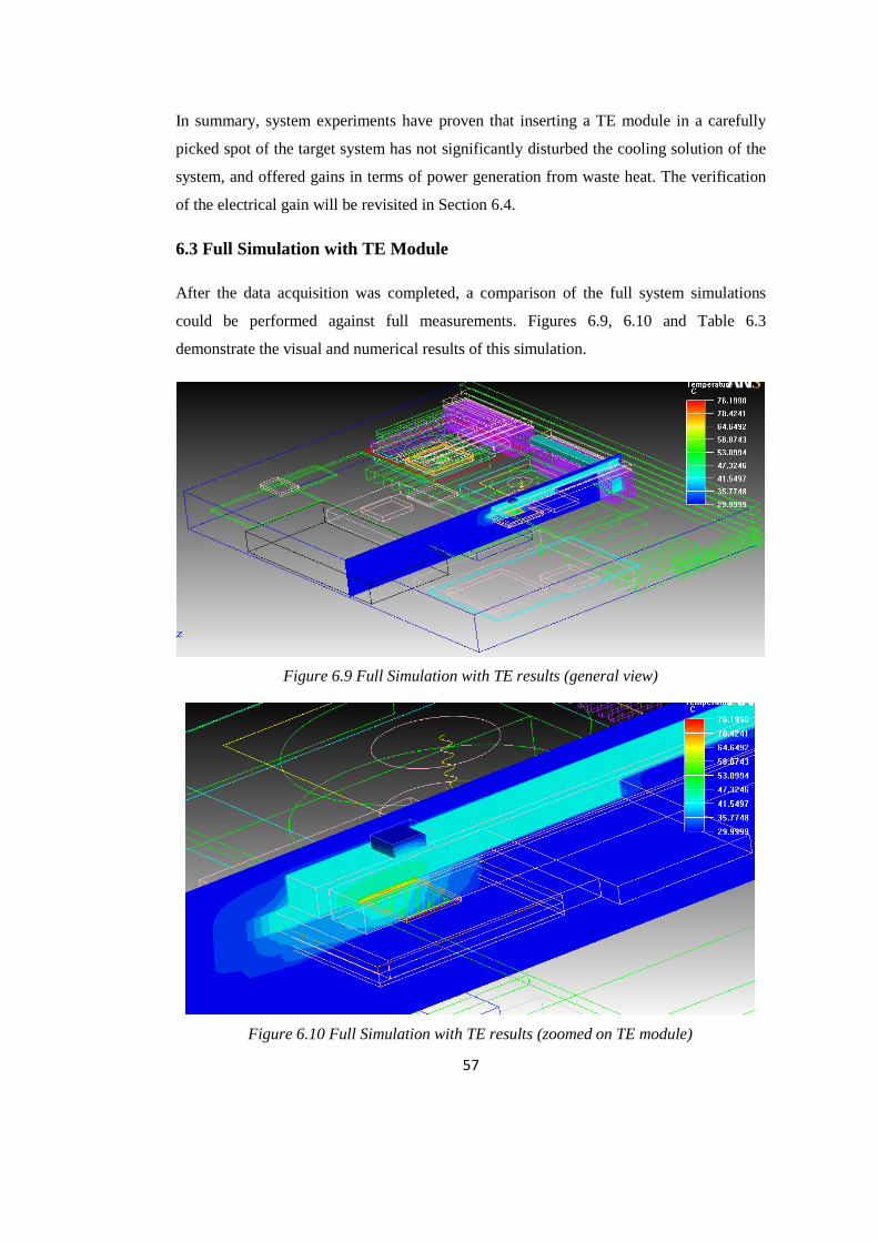
Figure 6.9 Full Simulation with TE results (general view)…………………………. 57
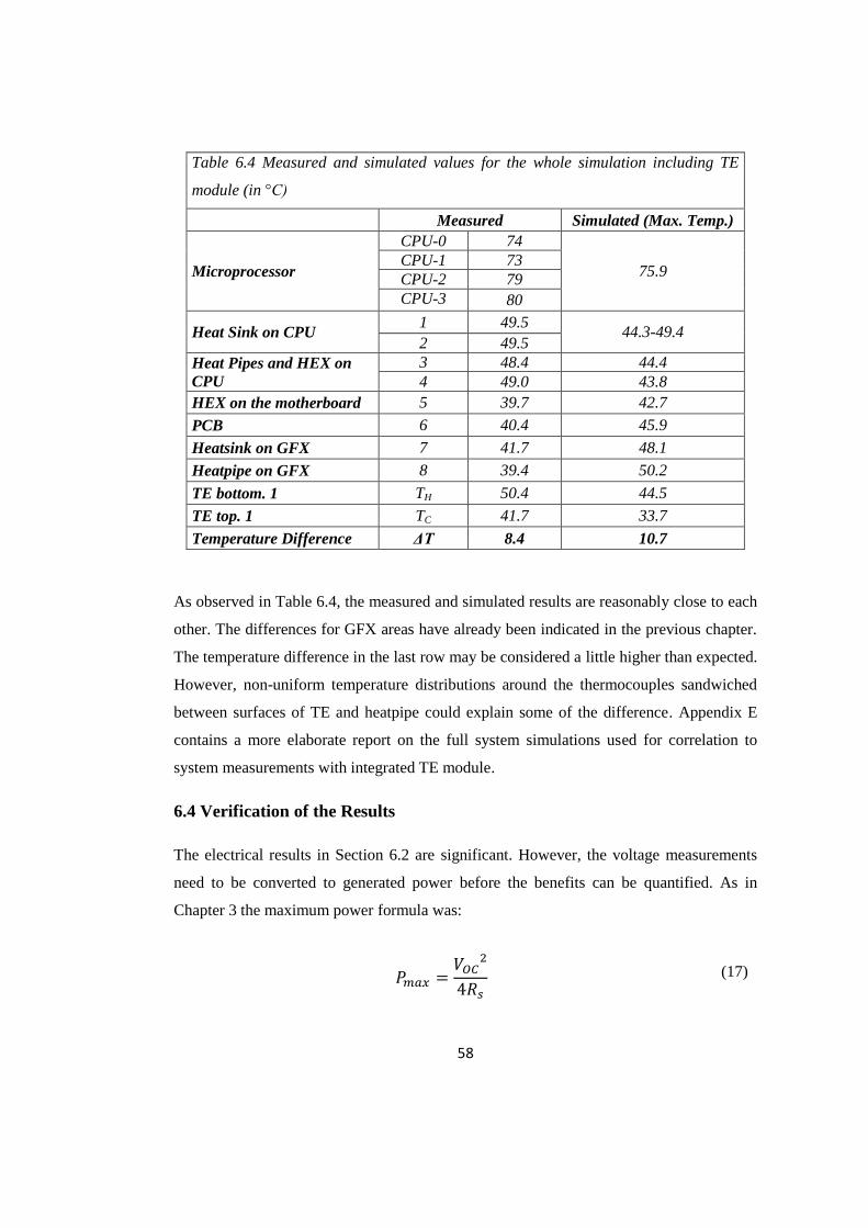
Figure 6.10 Full Simulation with TE results (zoomed on TE module)……………... 57
Figure 6.11 Temperature of CPU operating with 100% workload and the maximum
power generation possibilities by the TE module (6.05 mm 6.05mm x 2.59 mm)
over time………………………………………………………………………….
60
Figure 6.12 Thermal resistance cases……………………………………………….. 61
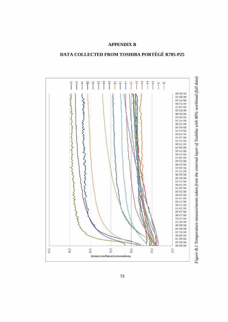
Figure B.1 Temperature measurements taken from the external layer of Toshiba
with 80% workload (full data)……………………………………………………
73
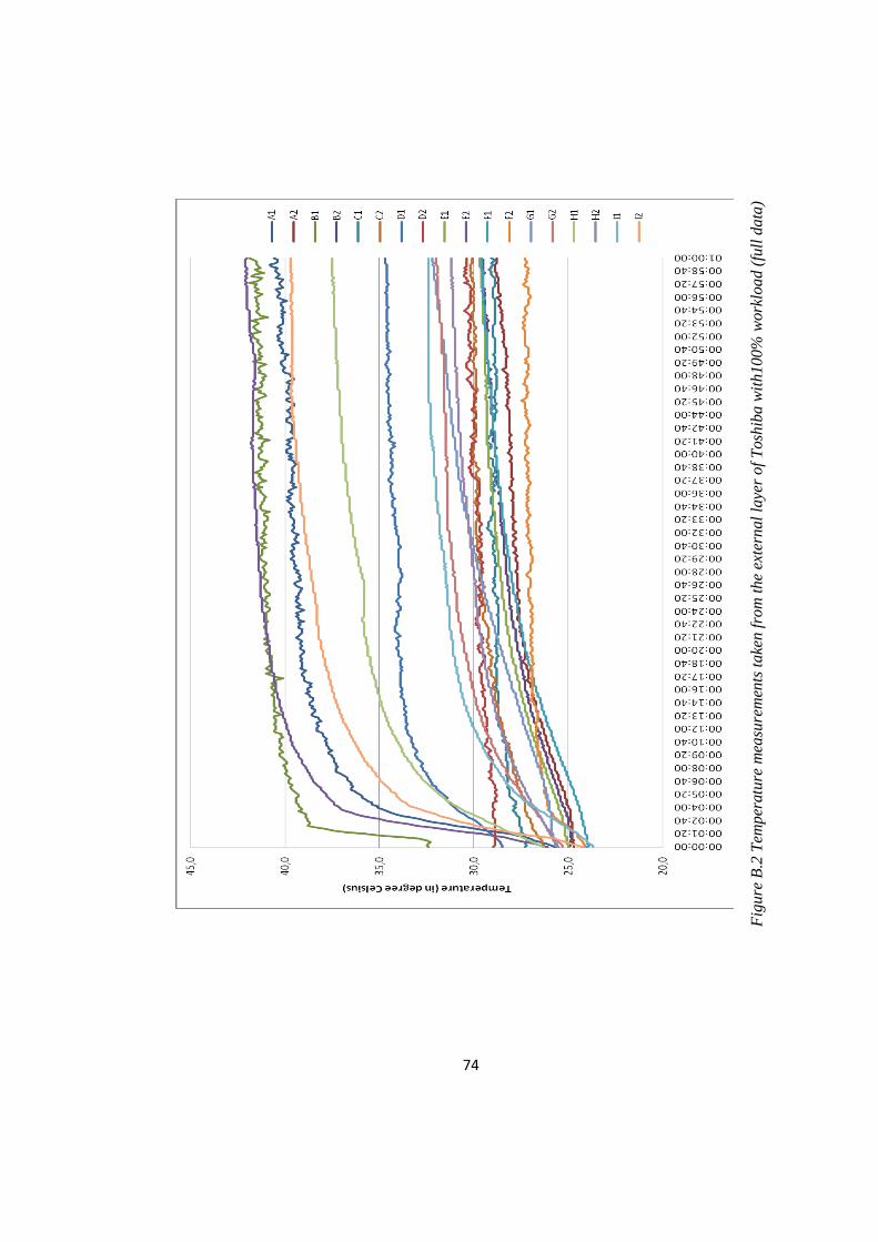
Figure B.2 Temperature measurements taken from the external layer of Toshiba
with100% workload (full data)…………………………………………………...
74
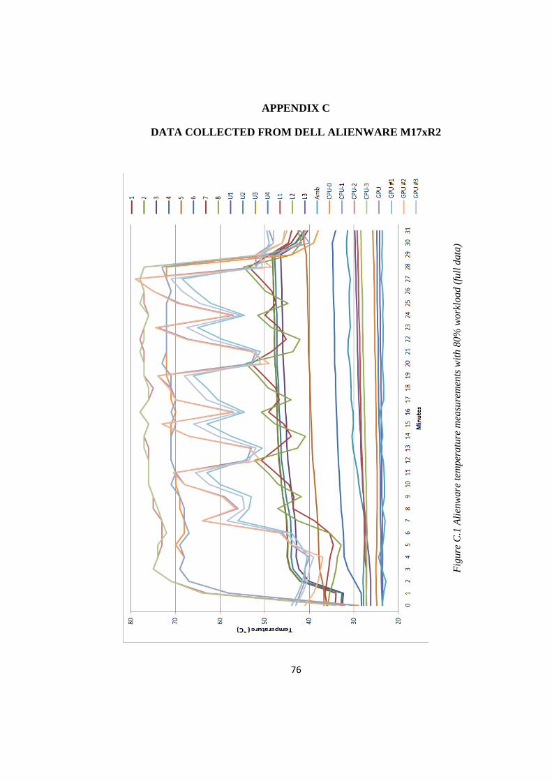
Figure C.1 Alienware temperature measurements with 80% workload (full data)…. 76
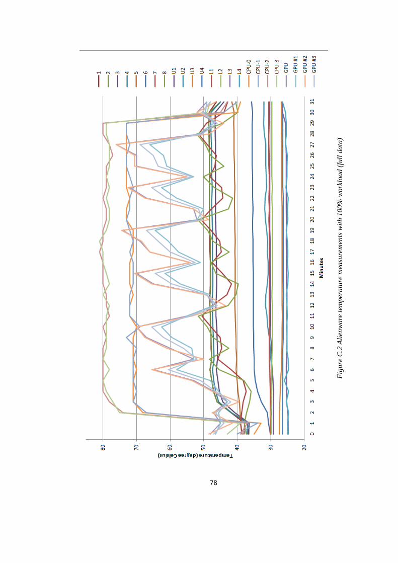
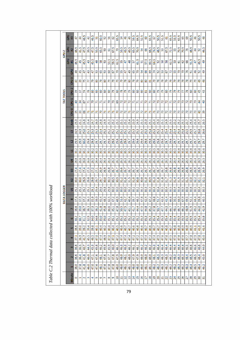
Figure C.2 Alienware temperature measurements with 100% workload (full data)... 78
Page 13
xiii
LIST OF TABLES
Table 4.1 Toshiba Portégé R705-P25 Specifications……………………….……..... 23
Table 4.2 Dell Alienware M17xR2 Specifications………………………………….. 24
Table 4.3 Energy scavenging opportunities using FerroTEC and TETECH modules
in different locations of Toshiba test system……………………………………..
31
Table 4.4 Energy scavenging opportunities using FerroTEC and TETECH module
in different locations of Alienware test system…………………………………..
39
Table 5.1 Measured and simulated values for CPU simulation……………………... 44
Table 5.2 Measured and simulated values for the whole simulation (in °C)………... 47
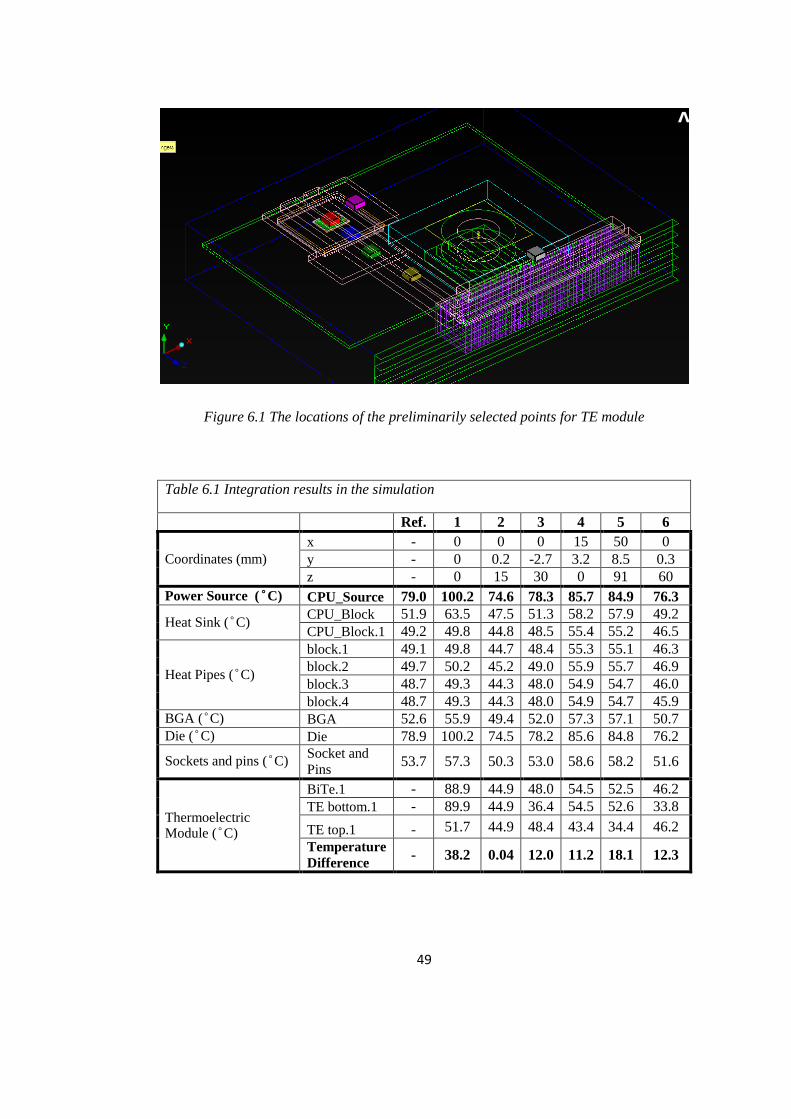
Table 6.1 Integration results in the simulation……………………………………… 49
Table 6.2 A comparison for the results obtained before and after the TE integration
on point 7…………………………………………………………………………
51
Table 6.3 Average Temperature of CPU in different scenarios…………………….. 55
Table 6.4 Measured and simulated values for the whole simulation including TE
module (in °C)……………………………………………………………………
58
Table 6.5 Maximum generated power by the TE module (6.05 mm x 6.05 mm x
2.59 mm) for different scenarios…………………………………………………
59
Table 6.6 Revised FerroTEC characterization values………………………………. 60
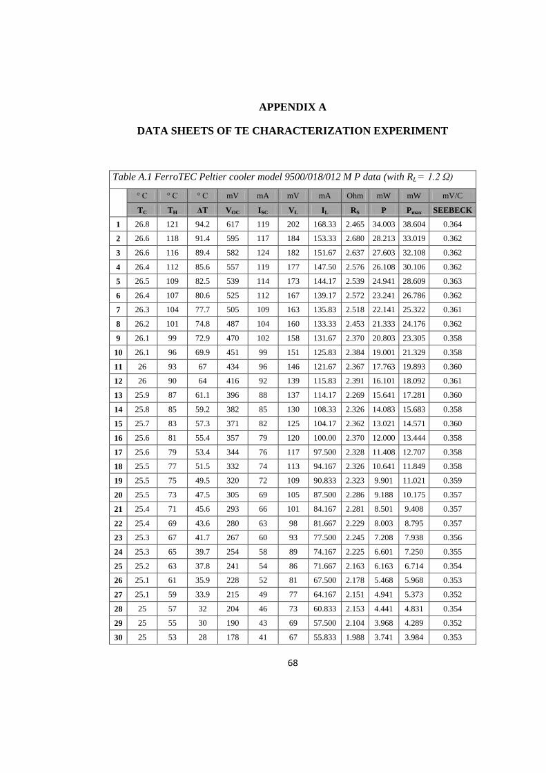
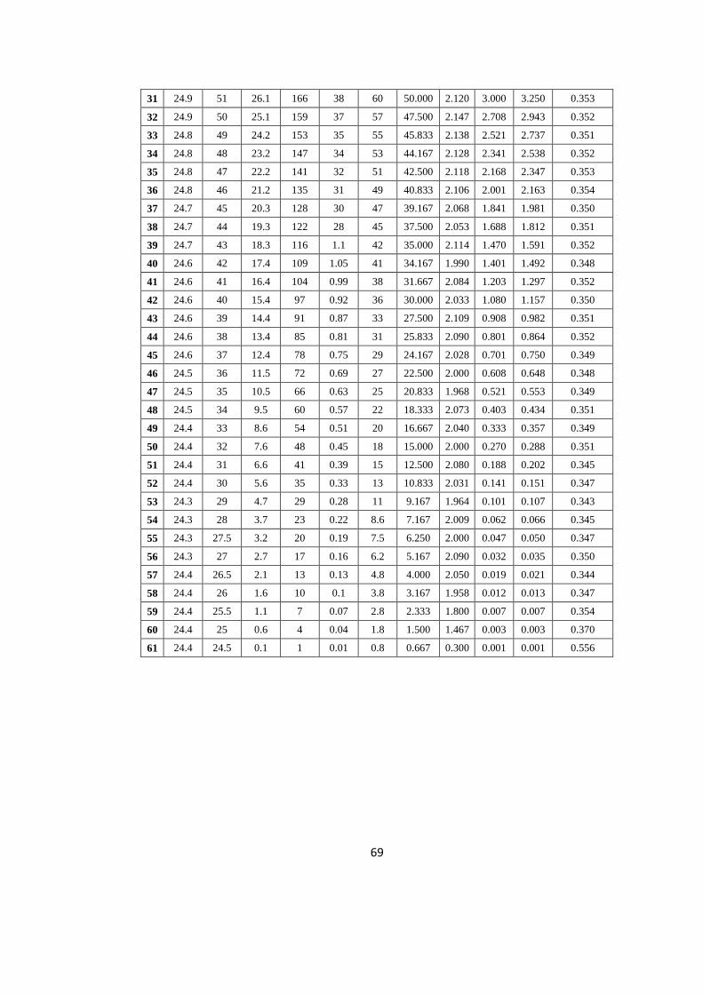
Table A.1 FerroTEC Peltier cooler model 9500/018/012 M P data……………….... 68
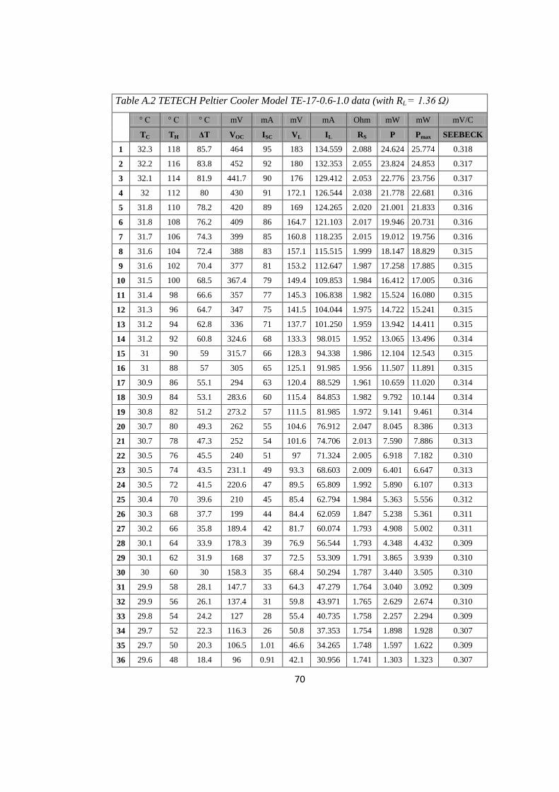
Table A.2 TETECH Peltier Cooler Model TE-17-0.6-1.0 data…………………….. 70
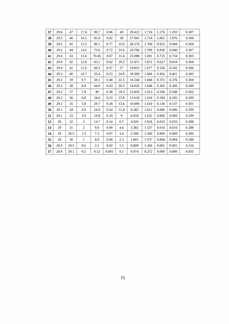
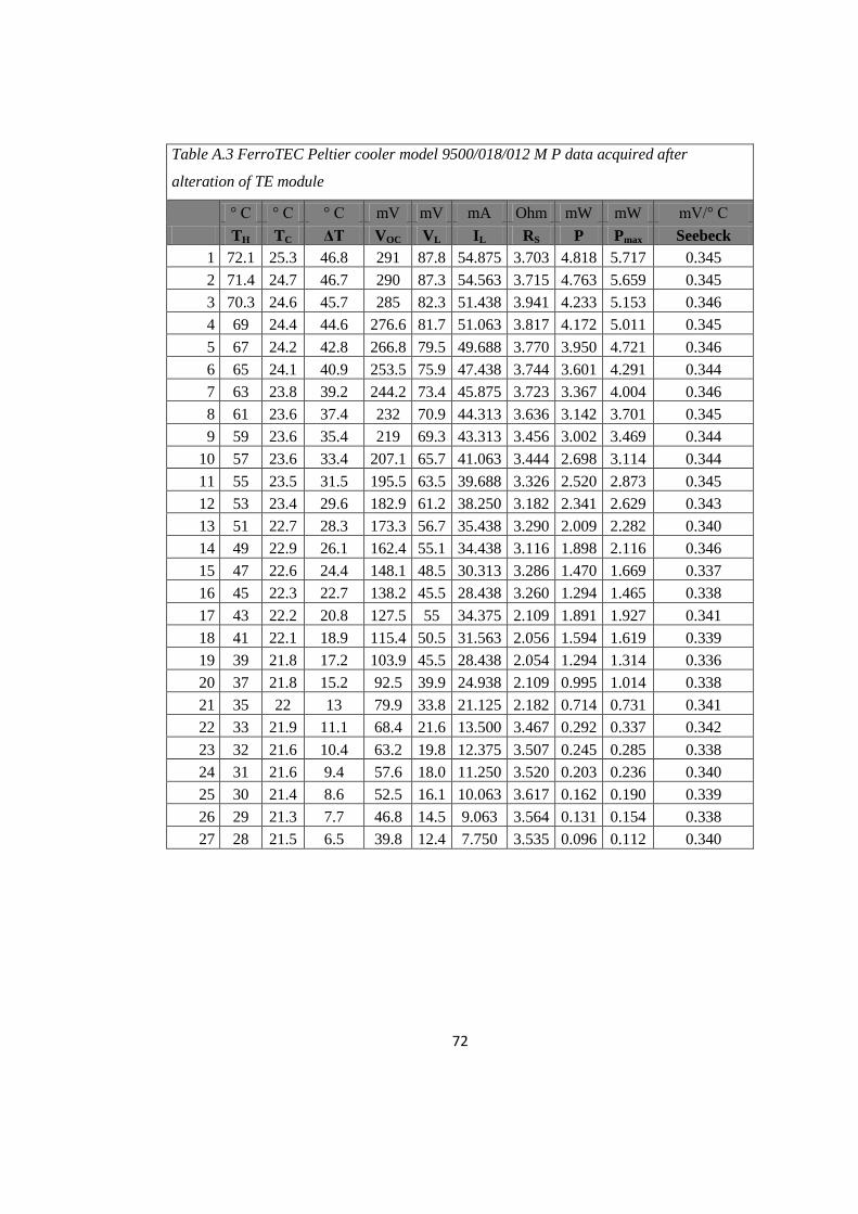
Table A.3 FerroTEC Peltier cooler model 9500/018/012 M P data acquired after
alteration of TE module…………………………………………………………..
72
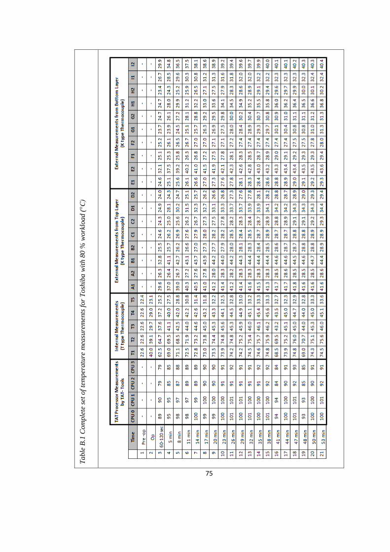
Table B.1 Complete set of temperature measurements for Toshiba with 80 %
workload (°C)……………………………………………………………………
75
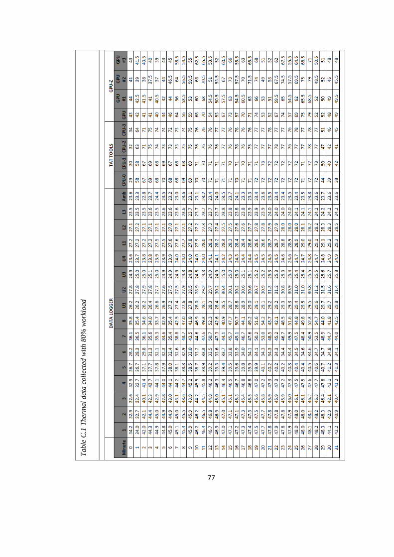
Table C.1 Thermal data collected with 80% workload…………………………….. 77
Table C.2 Thermal data collected with 100% workload…………………………… 79
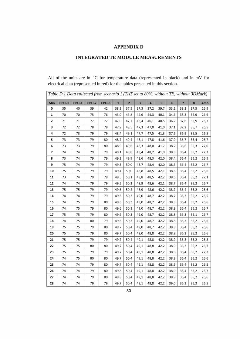
Table D.1 Data collected from scenario 1 (TAT set to 80%, without TE, without
3DMark)………………………………………………………………………….
80
Page 14
xiv
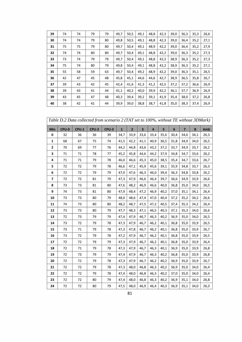
Table D.2 Data collected from scenario 2 (TAT set to 100%, without TE without
3DMark)………………………………………………………………………….
81
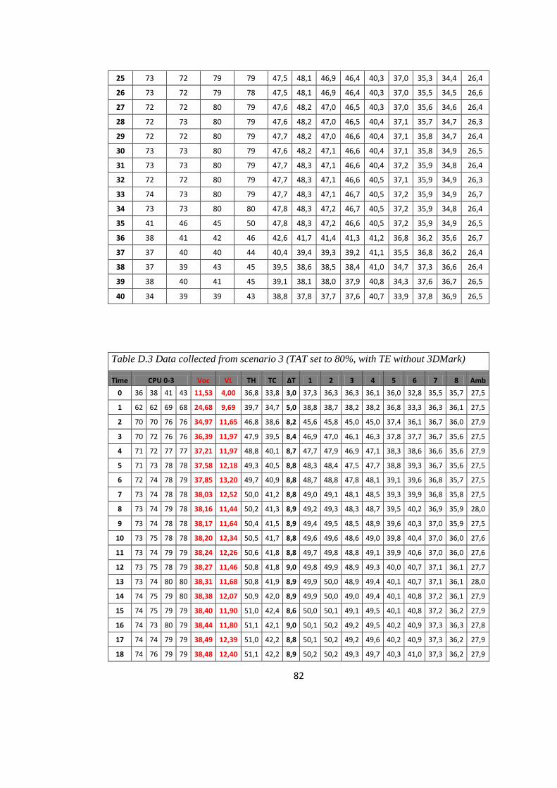
Table D.3 Data collected from scenario 3 (TAT set to 80%, with TE without
3DMark)………………………………………………………………………….
82
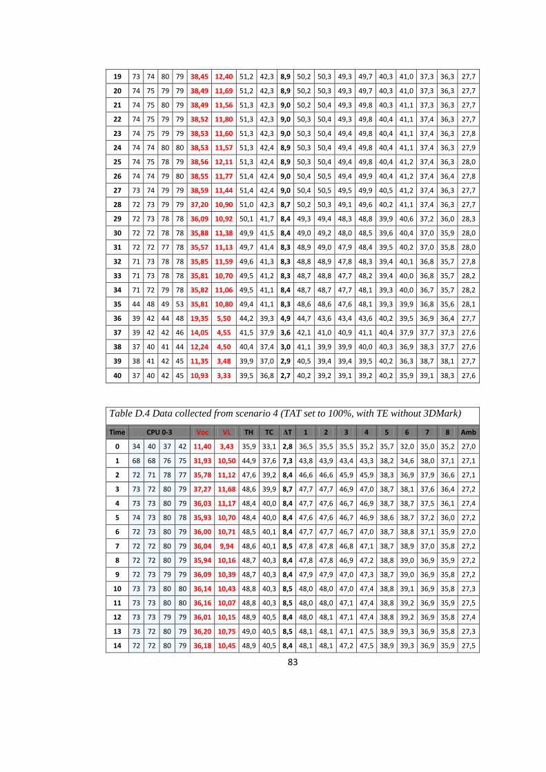
Table D.4 Data collected from scenario 4 (TAT set to 100%, with TE without
3DMark)………………………………………………………………………….
83
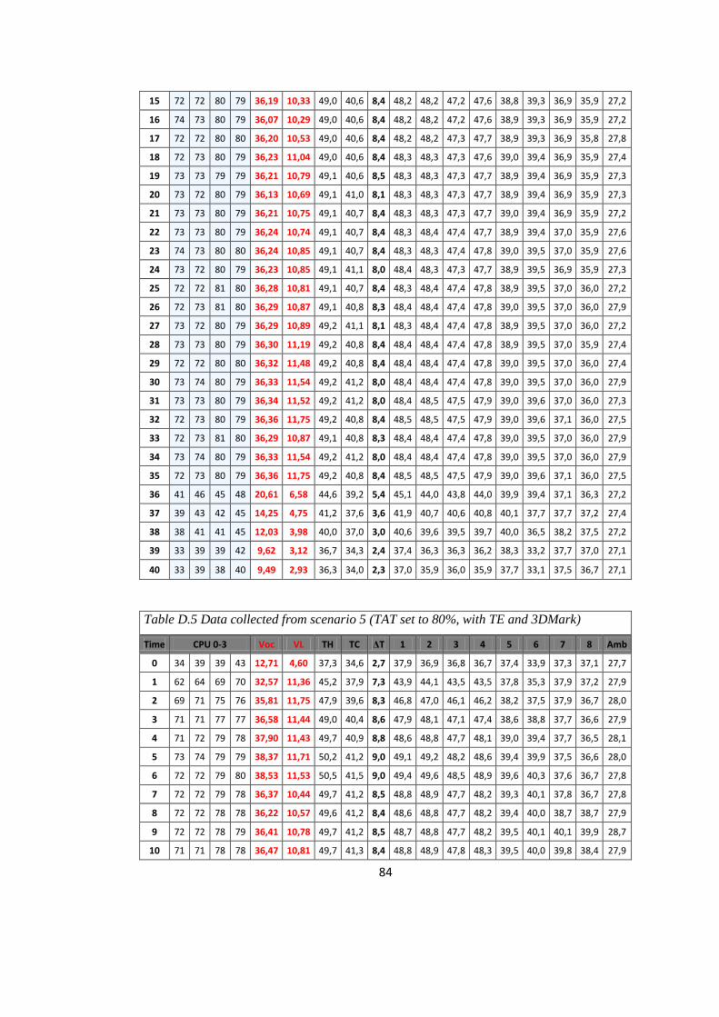
Table D.5 Data collected from scenario 5 (TAT set to 80%, with TE and 3DMark).. 84
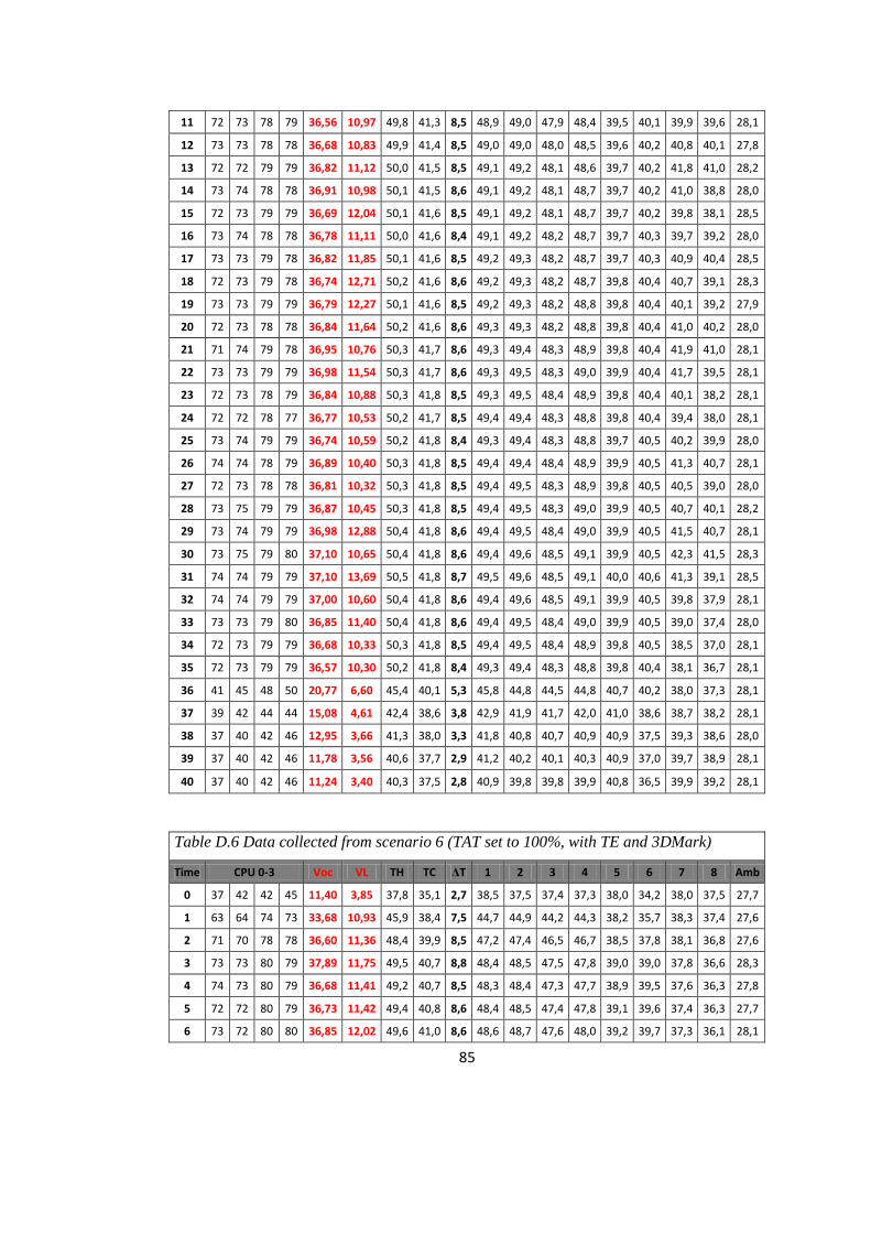
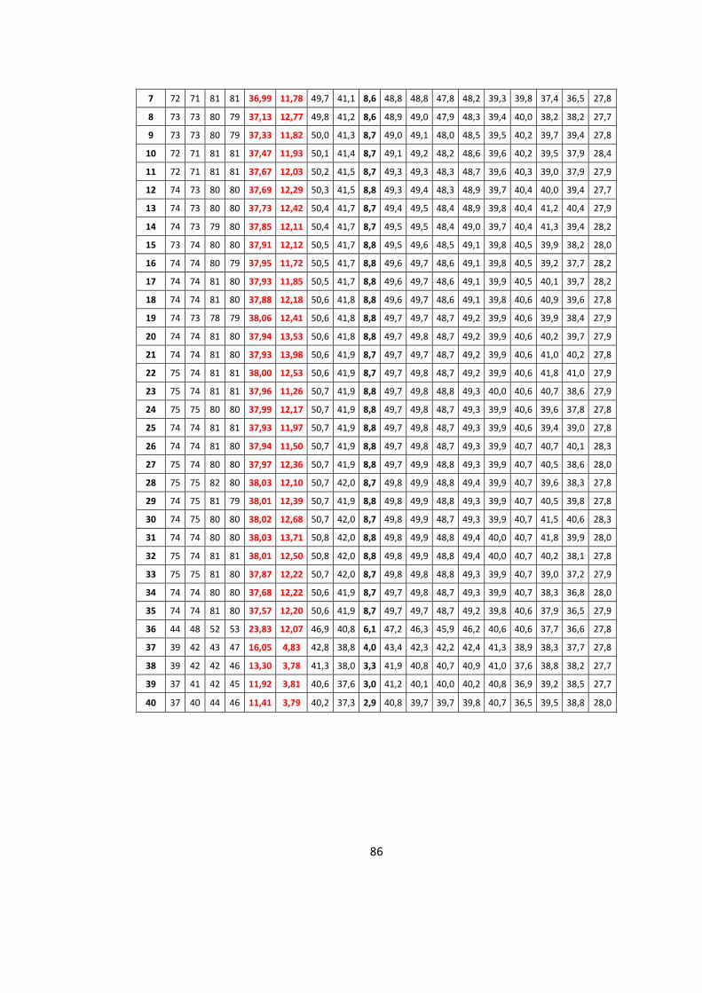
Table D.6 Data collected from scenario 6 (TAT set to 100%, with TE and 3DMark) 85
Table E.1 Overview of the Full Simulation without TE…………………………….. 87
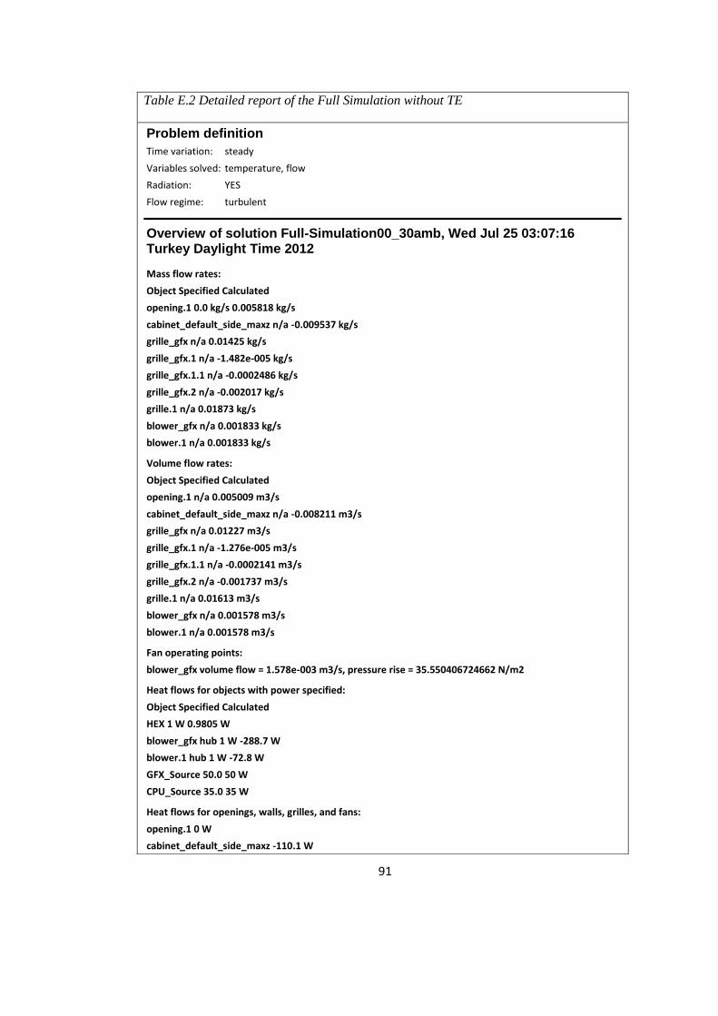
Table E.2 Detailed report of the Full Simulation without TE………………………. 91
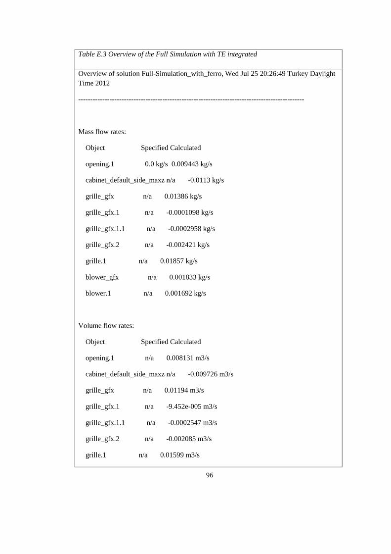
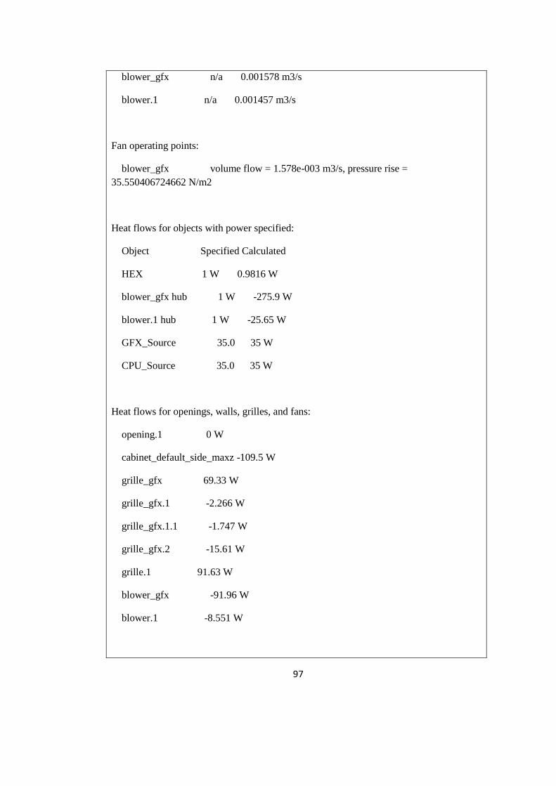
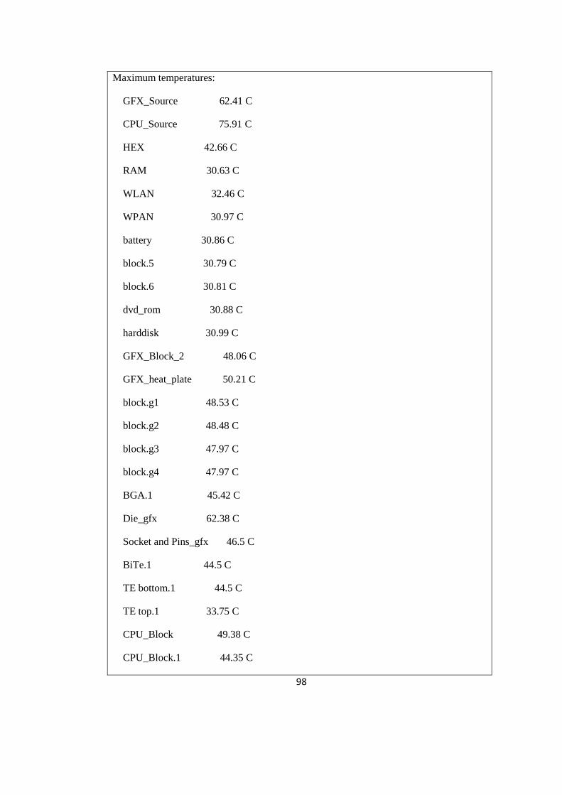
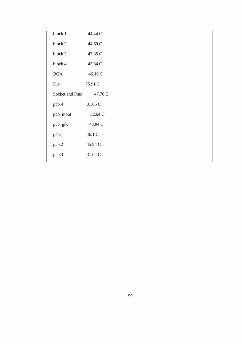
Table E.3 Overview of the Full Simulation with TE integrated…………………….. 96
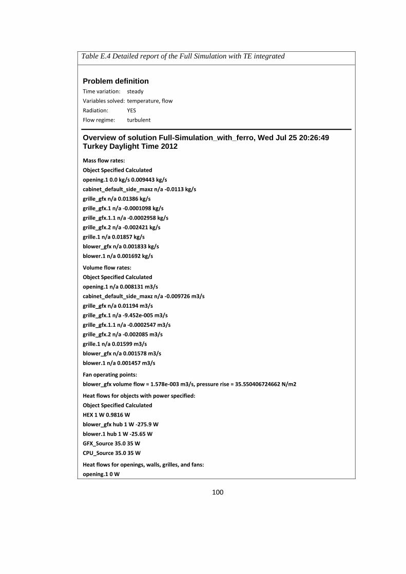
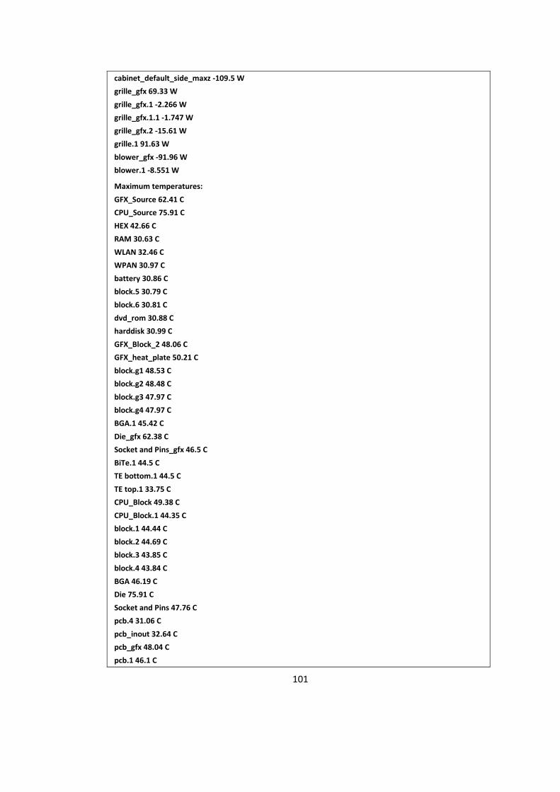
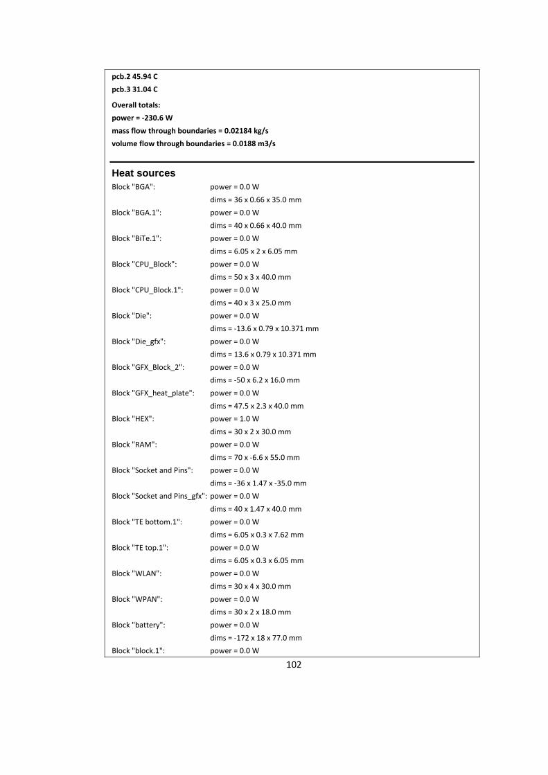
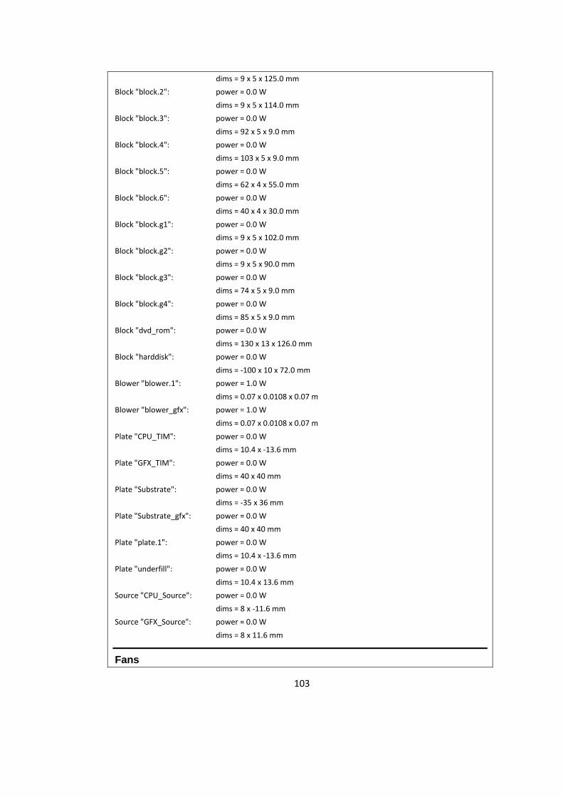
Table E.4 Detailed report of the Full Simulation with TE integrated……………….. 100
Page 15
xv
NOMENCLATURE
IL Loaded circuit current, (mA)
n Number of TE couples
P Power, (mW)
PF Power factor, (W/ K m2)
Pmax Maximum power, (mW)
RL Load resistance, (Ω)
RS Material resistance, (Ω)
TC Temperature of the cold surface, (°C)
TH Temperature of the hot surface, (°C)
V Voltage, (mV)
VL Loaded circuit voltage, (mV)
VOC Open circuit voltage, (mV)
ZT Dimensionless figure of merit
α Seebeck coefficient, (mV/°C)
ηC Carnot efficiency
κ Thermal conductivity, (W/K m)
ρ Electrical resistivity, (Ω m)
ψ Thermal resistance, (°C/W)
Page 16
1
CHAPTER 1
INTRODUCTION
1.1 Energy Harvesting
The power of energy acquisition has become a very important subject with the
contributions of the acceleratingly growing economy and day-by-day decreasing amount
of energy sources. On one hand, the continuing development of the technology increases
the energy demand. On the other, hand the conventional fossil fuel sources grow scarcer.
Therefore, more sustainable energy acquisition methods started to become a popular
research topic. Energy acquisition has turned into a troublesome task especially for
electrical and electronic devices, which keep becoming more prevalent, complex and
small each passing day. The current miniaturization trend makes the former energy
sources like batteries less functional, since their effectiveness also diminishes
proportionally with their geometry. Therefore the improvement of the battery life highly
depends on the reduction of the power consumption and battery dependency [1].
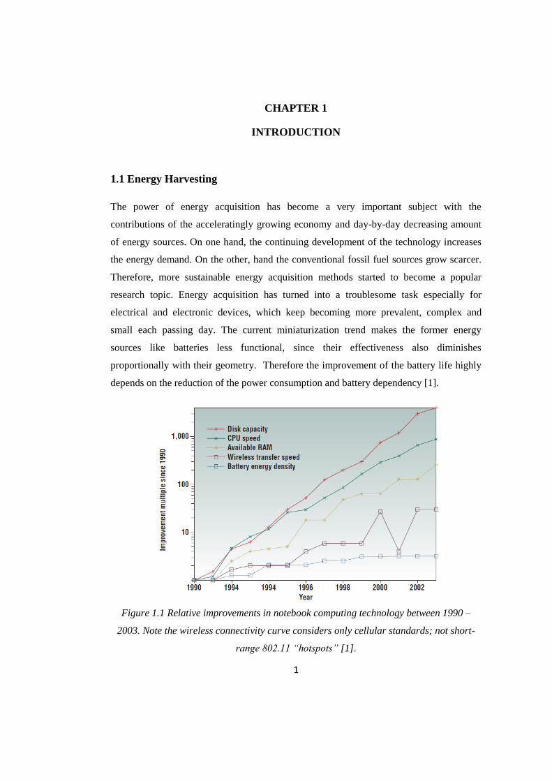
Figure 1.1 Relative improvements in notebook computing technology between 1990 –
2003. Note the wireless connectivity curve considers only cellular standards; not short-
range 802.11 “hotspots” [1].
Page 17
2
Figure 1.1 provides the recent development stages of different notebook components over
the years. It is apparent that the battery energy density has developed over the years as
well. However these improvements were quite small in comparison with the other parts.
Empowering the electronic devices using chemical reactions is an ongoing research topic.
Normal sized fuel cells seem to be too large to integrate into many models of electronic
devices, while microcells are proven to be too small to provide enough energy for
operating. There are additional options to solve the energy management problem in micro
scale electronics such as microturbines and microengines. Although their efficiencies of
power production are relatively high, they bring up additional problems like overheating,
noise and safety. Their degree of sustainability is also open to discussion since they work
on burning fuel [1]. A more detailed analysis in nanoscale energy harvesting has been
carried out by Wang [2], who reviewed many different energy harvesting technologies
with potential to power nano-systems.
As sustainability becomes an important part of the contemporary technological
developments for environmental and economical reasons, the concept of energy
scavenging offers a convenient solution. By definition, energy scavenging can be
described as the method to recover energy which was originally lost to the environment or
unusable. There are three major energy scavenging methods that utilize photovoltaic,
vibration and thermal gradient [3, 4]. Photovoltaic systems are designated to collect and
convert solar energy into electricity and can be applied to small electronic systems by
placing small panels outside the chassis. This has been a very common practice used in
many calculators for more than two decades, and recent developments in the photovoltaic
technology enable extension of the same principle to notebooks as well [5, 6].
Vibration based scavenging is generally used with the assistance of micro-scale
electromagnetic (EM) or piezoelectric (PZ) generators. EM generators have magnets on
top, and convert the fluctuations in the electromagnetic field into electrical voltage. There
are various applications like watches which have been developed to use the vibrations
created by human body as an energy source. Consisting of a piezoelectric element with a
resonantly matched transformer, piezoelectric generators can produce electricity under
vibration. It is possible to harvest energy from a computer keyboard, for example, to
supply the battery [1].
Page 18
3
The third major method for energy scavenging is the thermal gradient method. This
method is based upon using the heat difference between two surfaces as a power source in
order to harvest this energy with thermoelectric (TE) materials.
1.2 Thesis Objective
This thesis will analyze the energy scavenging options in notebook systems through the
utilization of thermoelectric materials. Notebooks are widespread technological devices
which have a broad range of uses in the modern society. Like most of the modern devices,
notebooks need electrical energy in order to operate and can only work for a limited time
with the power supplied by their batteries. Although notebook batteries are rechargeable,
it is a known fact that they have a limited lifespan and each time a battery has been
recharged this life span is shortened by a small amount. Initiatives like Energy Star has
caused a variety of power management features to be implemented in notebooks to reduce
dependence of power from the electrical outlets during idle and active periods. In addition,
dynamic control of the notebook features in a closed self-regulating loop required
different kinds of sensors to be integrated into these systems.
The main purpose of this research is to reduce the dependence of notebooks on electrical
outlets through thermoelectric generation without conceding from the operational
performance and quality. It is expected that the current efficiency of the thermoelectric
materials may result in modest power output [1, 3, 4, 5]. Yet, the present study focuses on
developing the methodology for quantifying all thermoelectric energy scavenging
opportunities in a spectrum of notebook platforms available today and tomorrow. It is
expected that the generated energy can be used to increase battery life, or power up small
distributed sensors around the system which only require modest power to operate.
The previous research and theoretical background is examined in Chapter 2 to establish
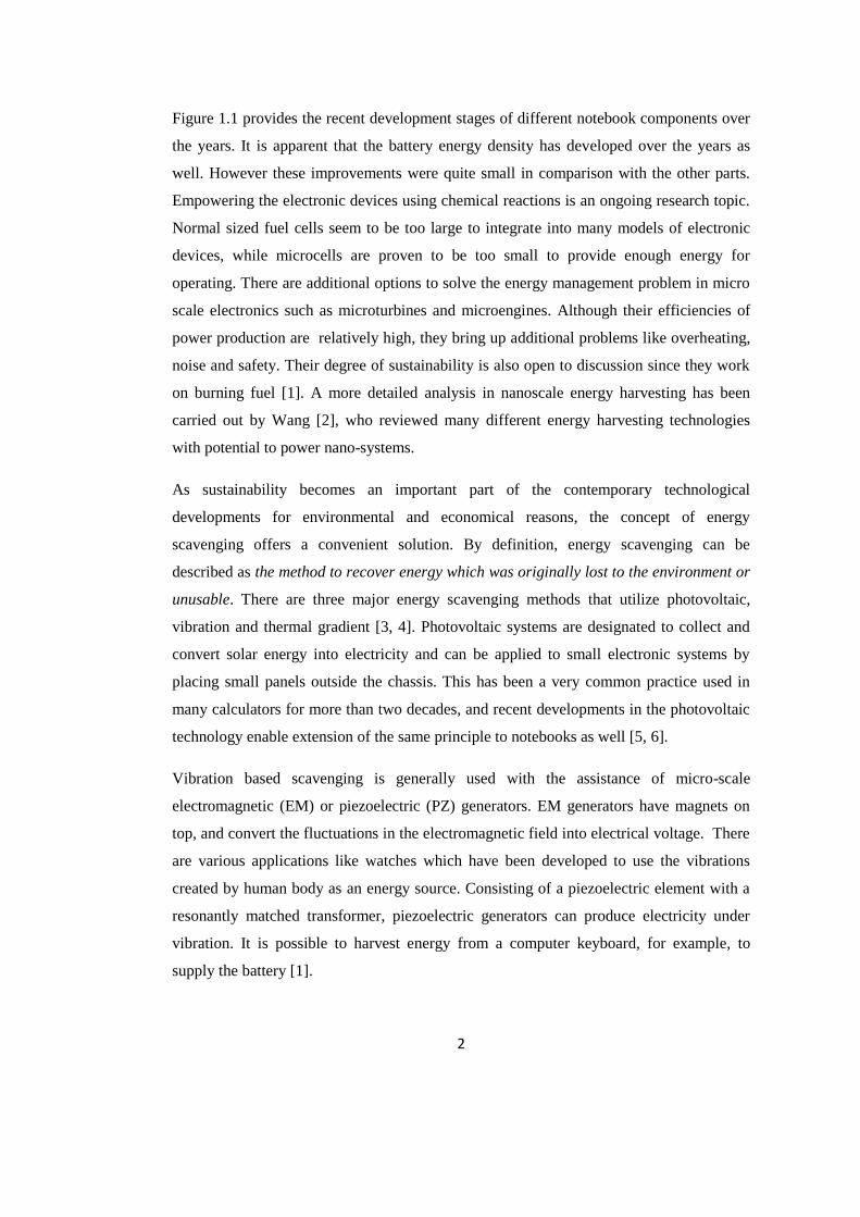
the relevance to the topic at hand. Figure 1.2 depicts the identified steps which were
followed throughout the research period for a healthy convergence to the system solution.
The experimentally based methodology behind this flow has been developed as part of
this thesis. Chapter 3 focuses on the TE characterization process including the
experimental methodology developed for this purpose. Chapter 4 covers the experimental
mechanical and thermal characterization of the target systems. After this point the
research focuses on one of the pre-evaluated target systems and TE modules. In Chapter 5,
Page 19
4
a partial and full CAD model of the selected system is presented. Chapter 6 focuses on the
TE integration analysis and its validation. Finally the conclusions from the thesis are
discussed in Chapter 7.
Figure 1.2 Steps in experimental development of TE generation in notebook systems
Page 20
5
CHAPTER 2
BACKGROUND AND PREVIOUS WORK
2.1 Background Research
2.1.1 Thermoelectric Modules
Thermoelectric (TE) modules are specially designed systems used to convert the thermal
gradient between two sides of a TE couple into a voltage difference by the Seebeck effect
or vice versa (which is generally referred as Peltier effect.) This phenomenon is
discovered in 1821 by Thomas Johann Seebeck, a German physicist, who had observed
that a circuit built between two different metals with junctions at different temperatures,
creates a voltage difference between those metals. The Seebeck effect can briefly be
expressed with the following equation:
(1)
Here TH stands for the temperature of the hot surface and TC at the cold surface. The
Seebeck coefficient α (unit mV/K) is the conversion factor between the temperature
gradient and the voltage. TE modules contain a pair of distinctly doped semi-conductors
(x and y) each with a different Seebeck coefficient of opposite sign. These two
coefficients can be combined as [7]:
(2)
However one must keep in mind that this is a rather simplified definition, as the Seebeck
coefficient itself is also temperature dependent and may vary according to the working
condition. This situation may pose a problem especially for large temperature differences,
thus rendering the equation less useful. However for cases, in which ΔT < 100°, those
changes are rather small, making a “constant α” assumption plausible.
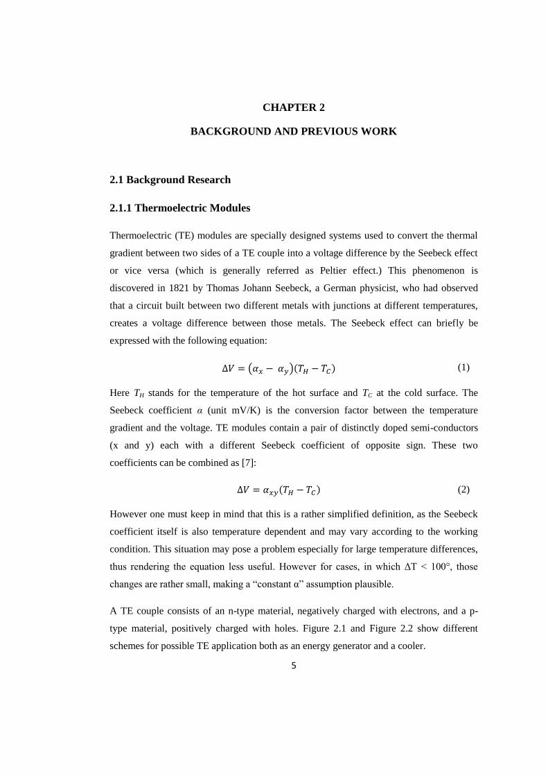
A TE couple consists of an n-type material, negatively charged with electrons, and a p-
type material, positively charged with holes. Figure 2.1 and Figure 2.2 show different
schemes for possible TE application both as an energy generator and a cooler.
Page 21
6
Figure 2.1 Thermoelectric couple in (a) cooler, and (b) generator configuration. [8]
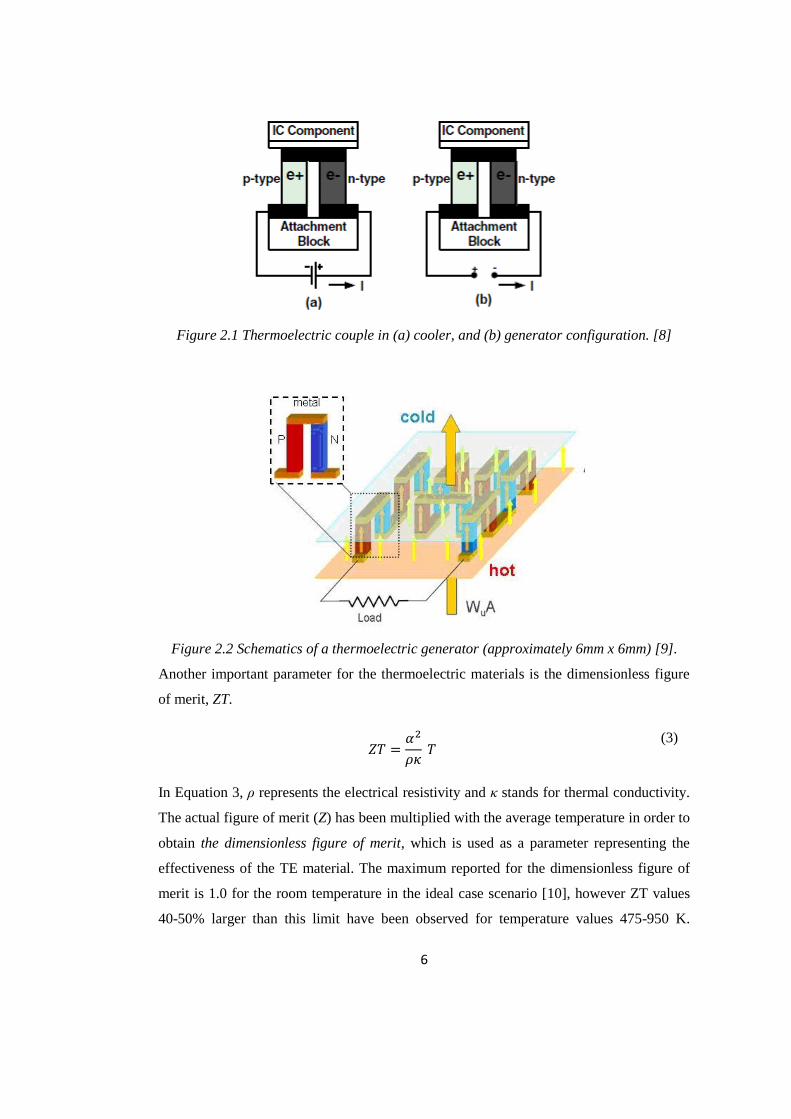
Figure 2.2 Schematics of a thermoelectric generator (approximately 6mm x 6mm) [9].
Another important parameter for the thermoelectric materials is the dimensionless figure
of merit, ZT.
(3)
In Equation 3, ρ represents the electrical resistivity and κ stands for thermal conductivity.
The actual figure of merit (Z) has been multiplied with the average temperature in order to
obtain the dimensionless figure of merit, which is used as a parameter representing the
effectiveness of the TE material. The maximum reported for the dimensionless figure of
merit is 1.0 for the room temperature in the ideal case scenario [10], however ZT values
40-50% larger than this limit have been observed for temperature values 475-950 K.
Page 22
7
Research in thermoelectric materials has shown that theoretical ZT values between 2.0-3.0
are possible [11].
This thesis deals with the internal temperatures of the mobile computers. As further
documented in the following chapters, this application has an available temperature range
of 25-110 °C under regular room conditions with 25 °C ambient. The most efficient
Seebeck coefficient in this range has been observed between Bi2Te3 (bismuth telluride) as
the n-type material and Sb2Te3 (antimony telluride) as the p-type material, which have
practically provided Seebeck coefficient between 0.3-0.4 mV/K, and dimensionless figure
of merit of 0.84-0.87 [10, 11, 12]. TE modules built using Bi2Te3 - Sb2Te3 couple is
known for their relatively high power generation potential even with a temperature
difference smaller than 10° C [13].
One of the reasons for this drop of efficiency in lower temperature difference can be
explained with Carnot efficiency. Although solid state thermoelectric generators have
many advantages like sustainability and being maintenance free, one must keep in mind
that they are still thermal devices working with the principles of heat-work conversion.
Therefore the laws of the thermodynamics have to be taken into consideration during the
analysis of the TE materials.
Δ
(4)
Carnot cycle is accepted as the ideal case where the maximum possible heat can be
converted into the work. Thus Carnot efficiency provides us with the maximum
percentage of work attainable from any kind of heat transfer. As it has been shown in
Equation 4, the temperature difference and the temperature of the hot surface play a
dominant role in the determination of the Carnot efficiency [14].
(5)
The power factor PF is another important parameter after the figure of merit. PF is
measured in Watts per Kelvin square per meter (W/K2 m). It carries an important role for
the thermoelectric converters because it shows the relationship between the Seebeck
coefficient and the electrical resistivity of a material, thus determining the electrical
performance of the thermoelectric materials [10].
Page 23
8
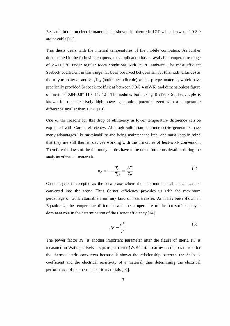
Thermotunnel effect has also been an important thermal based energy scavenging method
aside from the Seebeck effect. This phenomenon has been first observed in 1980’s by an
experiment in Al-PbBi tunnel-junctions and many experiments followed the first one
especially in the cooling applications. In thermotunnel coolers, two metallic grades are
being held separately with a vacuum in between and a bias voltage is applied to operate
the device. Acting like a Schottky barrier, the bias voltage creates a barrier between the
metals, thus disabling the electron transfer from the hot to the cold side, and enhancing the
tunneling effect in the other direction (Figure 2.3). Depresse and Jager argued that
thermotunneling devices have a much higher power density and thermal insulation
capabilities, thus making them better coolers than TE devices. However, they are not so
efficient for the energy scavenging opportunities due to weak voltage output and
conversion efficiency. It has been stated that even if the difficulties in the development
process can be overcome, the output voltage will be one magnitude lower than the
thermoelectric devices, thus making them unsuitable for this project [15].
Figure 2.3 Potential barrier Vh(xh) profile between electrodes with different
temperatures and electrode work functions. The solid line is the real potential profile
taking into account the image charge correction, the dotted one is the trapezoidal
approximation without correction [15].
Page 24
9
2.1.2 Applications in Microelectronic Systems
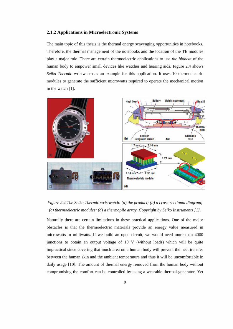
The main topic of this thesis is the thermal energy scavenging opportunities in notebooks.
Therefore, the thermal management of the notebooks and the location of the TE modules
play a major role. There are certain thermoelectric applications to use the bioheat of the
human body to empower small devices like watches and hearing aids. Figure 2.4 shows
Seiko Thermic wristwatch as an example for this application. It uses 10 thermoelectric
modules to generate the sufficient microwatts required to operate the mechanical motion
in the watch [1].
Figure 2.4 The Seiko Thermic wristwatch: (a) the product; (b) a cross-sectional diagram;
(c) thermoelectric modules; (d) a thermopile array. Copyright by Seiko Instruments [1].
Naturally there are certain limitations in these practical applications. One of the major
obstacles is that the thermoelectric materials provide an energy value measured in
microwatts to milliwatts. If we build an open circuit, we would need more than 4000
junctions to obtain an output voltage of 10 V (without loads) which will be quite
impractical since covering that much area on a human body will prevent the heat transfer
between the human skin and the ambient temperature and thus it will be uncomfortable in
daily usage [10]. The amount of thermal energy removed from the human body without
compromising the comfort can be controlled by using a wearable thermal-generator. Yet
Page 25
10
in most cases the thermoelectric generators are used as an additional source instead of
replacing batteries.
This methodology becomes rather attractive especially in microsystems which rely on
batteries with a limited life span. The continuously decreasing geometry of the new
battery models have hard time catching up with the power density requirements of the
current technology. In certain cases, replacing those batteries can also prove to be an
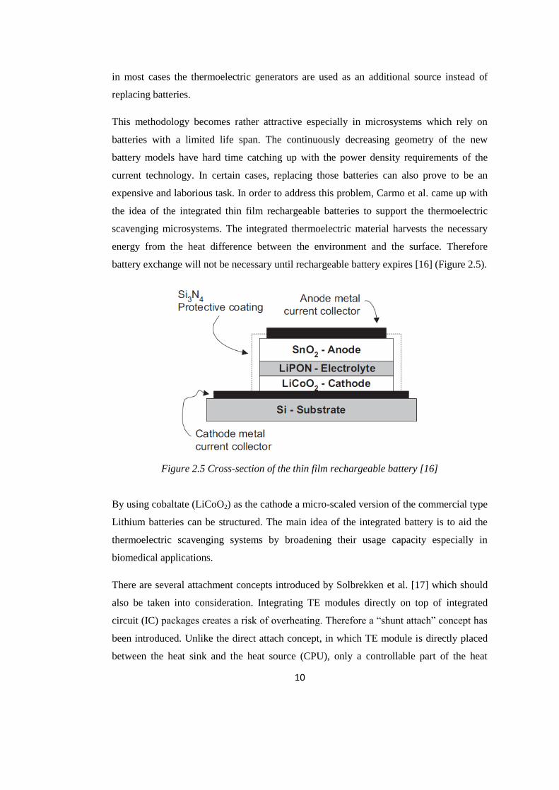
expensive and laborious task. In order to address this problem, Carmo et al. came up with
the idea of the integrated thin film rechargeable batteries to support the thermoelectric
scavenging microsystems. The integrated thermoelectric material harvests the necessary
energy from the heat difference between the environment and the surface. Therefore
battery exchange will not be necessary until rechargeable battery expires [16] (Figure 2.5).
Figure 2.5 Cross-section of the thin film rechargeable battery [16]
By using cobaltate (LiCoO2) as the cathode a micro-scaled version of the commercial type
Lithium batteries can be structured. The main idea of the integrated battery is to aid the
thermoelectric scavenging systems by broadening their usage capacity especially in
biomedical applications.
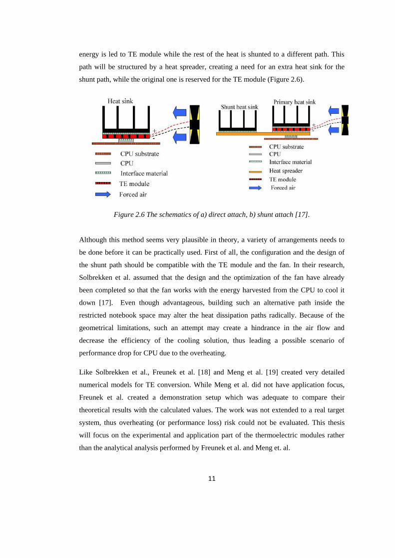
There are several attachment concepts introduced by Solbrekken et al. [17] which should
also be taken into consideration. Integrating TE modules directly on top of integrated
circuit (IC) packages creates a risk of overheating. Therefore a “shunt attach” concept has
been introduced. Unlike the direct attach concept, in which TE module is directly placed
between the heat sink and the heat source (CPU), only a controllable part of the heat
Page 26
11
energy is led to TE module while the rest of the heat is shunted to a different path. This
path will be structured by a heat spreader, creating a need for an extra heat sink for the
shunt path, while the original one is reserved for the TE module (Figure 2.6).
Figure 2.6 The schematics of a) direct attach, b) shunt attach [17].
Although this method seems very plausible in theory, a variety of arrangements needs to
be done before it can be practically used. First of all, the configuration and the design of
the shunt path should be compatible with the TE module and the fan. In their research,
Solbrekken et al. assumed that the design and the optimization of the fan have already
been completed so that the fan works with the energy harvested from the CPU to cool it
down [17]. Even though advantageous, building such an alternative path inside the
restricted notebook space may alter the heat dissipation paths radically. Because of the
geometrical limitations, such an attempt may create a hindrance in the air flow and
decrease the efficiency of the cooling solution, thus leading a possible scenario of
performance drop for CPU due to the overheating.
Like Solbrekken et al., Freunek et al. [18] and Meng et al. [19] created very detailed
numerical models for TE conversion. While Meng et al. did not have application focus,
Freunek et al. created a demonstration setup which was adequate to compare their
theoretical results with the calculated values. The work was not extended to a real target
system, thus overheating (or performance loss) risk could not be evaluated. This thesis
will focus on the experimental and application part of the thermoelectric modules rather
than the analytical analysis performed by Freunek et al. and Meng et. al.
Page 27
12
Hsu et al. [20] found a niche for TE harvesting in the exhaust system of the automobiles.
They naturally dealt with much higher temperature and power levels in that particular
application compared to what is available in a microelectronic system, but they have
practically used an existing shunt path for heat dissipation, same concept as previously
described.
The specifications and thermal characterization of TE modules also bear an important role
in the energy scavenging systems. The paper by Niu et al. [21] includes a detailed analysis
about how different commercially available TE generators act under various external
conditions. However, the introduced experimental model seems too detailed for the scope
of this research. Because it includes many different parameters on different scenarios
which have no direct influence upon the system at hand. Thus a self-built TE
characterization model inspired by the work of Muhtaroğlu et al. [8] will be used in this
project.
Energy scavenging is an important part of sustainable energy technologies which can be
utilized in computer and electronics branches. A study conducted by Mathuna et al. [22]
shows the application possibilities for different energy scavenging methodologies in
wireless sensor networks. This study is a good reference for a sequel research project to
this thesis focusing on the utilization of the harvested energy in notebooks.
2.2 Previous Work
Some previously developed ideas about the thermoelectricity and heat management in
microelectronic systems and other applications have been presented in the previous
section. Although they were based on the same theories and principles they provided a
general idea about the current condition of the state-of-the-art. In this section, however,
the focus will be on two specific papers (Muhtaroğlu et al. [8] and Rocha et al. [12])
which followed the same or similar aim as this project, and therefore can be accepted as
predecessors.
The first paper, written by Muhtaroğlu et al. [8], examined hybrid thermoelectric
conversion. Two different cases were highlighted to focus on the average and maximum
power usage in mobile computers. It was assumed that mobile computers spend 15% of
their lifetime in maximum operation condition. This state is called thermal design power
because the cooling solution is designed for this condition. The remaining 85% is assumed
Page 28
13
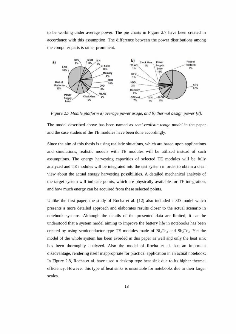
to be working under average power. The pie charts in Figure 2.7 have been created in
accordance with this assumption. The difference between the power distributions among
the computer parts is rather prominent.
Figure 2.7 Mobile platform a) average power usage, and b) thermal design power [8].
The model described above has been named as semi-realistic usage model in the paper
and the case studies of the TE modules have been done accordingly.
Since the aim of this thesis is using realistic situations, which are based upon applications
and simulations, realistic models with TE modules will be utilized instead of such
assumptions. The energy harvesting capacities of selected TE modules will be fully
analyzed and TE modules will be integrated into the test system in order to obtain a clear
view about the actual energy harvesting possibilities. A detailed mechanical analysis of
the target system will indicate points, which are physically available for TE integration,
and how much energy can be acquired from these selected points.
Unlike the first paper, the study of Rocha et al. [12] also included a 3D model which
presents a more detailed approach and elaborates results closer to the actual scenario in
notebook systems. Although the details of the presented data are limited, it can be
understood that a system model aiming to improve the battery life in notebooks has been
created by using semiconductor type TE modules made of Bi2Te3 and Sb2Te3. Yet the
model of the whole system has been avoided in this paper as well and only the heat sink
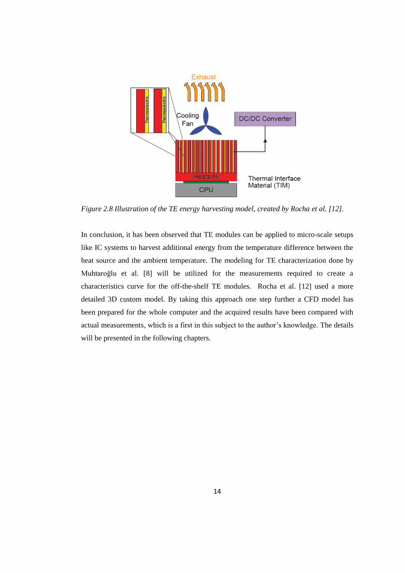
has been thoroughly analyzed. Also the model of Rocha et al. has an important
disadvantage, rendering itself inappropriate for practical application in an actual notebook:
In Figure 2.8, Rocha et al. have used a desktop type heat sink due to its higher thermal
efficiency. However this type of heat sinks is unsuitable for notebooks due to their larger
scales.
Page 29
14
Figure 2.8 Illustration of the TE energy harvesting model, created by Rocha et al. [12].
In conclusion, it has been observed that TE modules can be applied to micro-scale setups
like IC systems to harvest additional energy from the temperature difference between the
heat source and the ambient temperature. The modeling for TE characterization done by
Muhtaroğlu et al. [8] will be utilized for the measurements required to create a
characteristics curve for the off-the-shelf TE modules. Rocha et al. [12] used a more
detailed 3D custom model. By taking this approach one step further a CFD model has
been prepared for the whole computer and the acquired results have been compared with
actual measurements, which is a first in this subject to the author’s knowledge. The details
will be presented in the following chapters.
Page 30
15
CHAPTER 3
CHARACTERIZATION OF THERMOELECTRIC MODULES
In this chapter the characterization steps of the TE modules will be explained. Two
different off-the-shelf model TE modules have been selected for the characterization
process. Off-the-shelf models were preferred for their superior quality and ease of
availability. The selected TE modules are:
FerroTEC Peltier cooler model 9500/018/012 M P [23, 24]
TETECH TE 17-0.6-1.0 Thermoelectric Module [25]
These modules are originally designed to be small scaled Peltier coolers for a variety of
uses. As explained in Chapter 2, TE materials can be used in both ways. Therefore they
will be utilized as Seebeck generators.
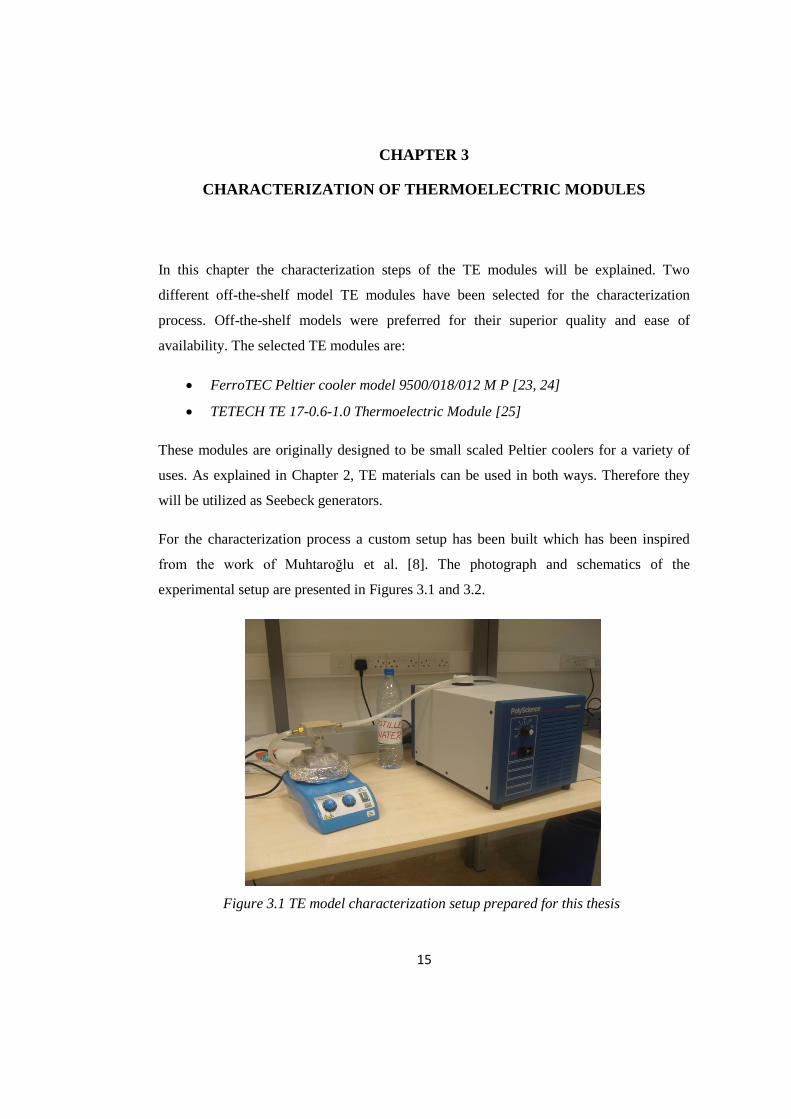
For the characterization process a custom setup has been built which has been inspired
from the work of Muhtaroğlu et al. [8]. The photograph and schematics of the
experimental setup are presented in Figures 3.1 and 3.2.
Figure 3.1 TE model characterization setup prepared for this thesis
Page 31
16
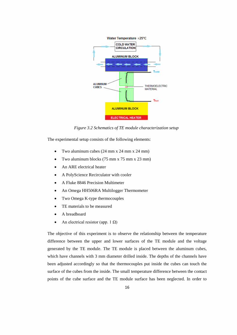
Figure 3.2 Schematics of TE module characterization setup
The experimental setup consists of the following elements:
Two aluminum cubes (24 mm x 24 mm x 24 mm)
Two aluminum blocks (75 mm x 75 mm x 23 mm)
An ARE electrical heater
A PolyScience Recirculator with cooler
A Fluke 8846 Precision Multimeter
An Omega HH506RA Multilogger Thermometer
Two Omega K-type thermocouples
TE materials to be measured
A breadboard
An electrical resistor (app. 1 Ω)
The objective of this experiment is to observe the relationship between the temperature
difference between the upper and lower surfaces of the TE module and the voltage
generated by the TE module. The TE module is placed between the aluminum cubes,
which have channels with 3 mm diameter drilled inside. The depths of the channels have
been adjusted accordingly so that the thermocouples put inside the cubes can touch the
surface of the cubes from the inside. The small temperature difference between the contact
points of the cube surface and the TE module surface has been neglected. In order to
Page 32
17
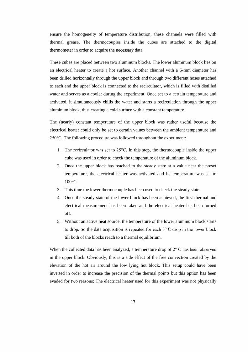
ensure the homogeneity of temperature distribution, these channels were filled with
thermal grease. The thermocouples inside the cubes are attached to the digital
thermometer in order to acquire the necessary data.
These cubes are placed between two aluminum blocks. The lower aluminum block lies on
an electrical heater to create a hot surface. Another channel with a 6-mm diameter has
been drilled horizontally through the upper block and through two different hoses attached
to each end the upper block is connected to the recirculator, which is filled with distilled
water and serves as a cooler during the experiment. Once set to a certain temperature and
activated, it simultaneously chills the water and starts a recirculation through the upper
aluminum block, thus creating a cold surface with a constant temperature.
The (nearly) constant temperature of the upper block was rather useful because the
electrical heater could only be set to certain values between the ambient temperature and
250°C. The following procedure was followed throughout the experiment:
1. The recirculator was set to 25°C. In this step, the thermocouple inside the upper
cube was used in order to check the temperature of the aluminum block.
2. Once the upper block has reached to the steady state at a value near the preset
temperature, the electrical heater was activated and its temperature was set to
100°C.
3. This time the lower thermocouple has been used to check the steady state.
4. Once the steady state of the lower block has been achieved, the first thermal and
electrical measurement has been taken and the electrical heater has been turned
off.
5. Without an active heat source, the temperature of the lower aluminum block starts
to drop. So the data acquisition is repeated for each 3° C drop in the lower block
till both of the blocks reach to a thermal equilibrium.
When the collected data has been analyzed, a temperature drop of 2° C has been observed
in the upper block. Obviously, this is a side effect of the free convection created by the
elevation of the hot air around the low lying hot block. This setup could have been
inverted in order to increase the precision of the thermal points but this option has been
evaded for two reasons: The electrical heater used for this experiment was not physically
Page 33
18
suitable to operate upside down and the error is expected to be insignificant due to the
present setup, thus it has been neglected.
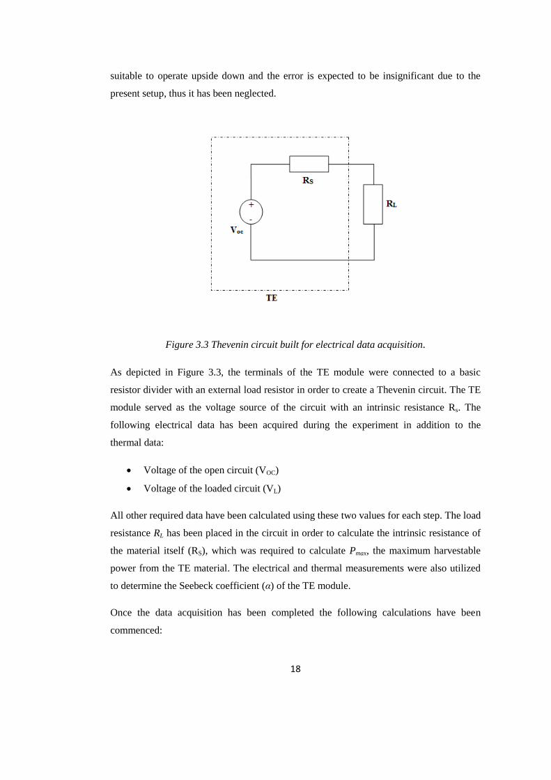
Figure 3.3 Thevenin circuit built for electrical data acquisition.
As depicted in Figure 3.3, the terminals of the TE module were connected to a basic
resistor divider with an external load resistor in order to create a Thevenin circuit. The TE
module served as the voltage source of the circuit with an intrinsic resistance Rs. The
following electrical data has been acquired during the experiment in addition to the
thermal data:
Voltage of the open circuit (VOC)
Voltage of the loaded circuit (VL)
All other required data have been calculated using these two values for each step. The load
resistance RL has been placed in the circuit in order to calculate the intrinsic resistance of
the material itself (RS), which was required to calculate Pmax, the maximum harvestable
power from the TE material. The electrical and thermal measurements were also utilized
to determine the Seebeck coefficient (α) of the TE module.
Once the data acquisition has been completed the following calculations have been
commenced:
Page 34
19
(6)
(7)
(8)
The power calculated here is the momentarily obtained power. However, the maximum
power can only be achieved when the resistance of the material equals the resistance of
the load.
(9)
(10)
(11)
In order to find the module Seebeck coefficient, the open circuit voltage has to be divided
to the measured temperature difference. Considering there are a number of TE couples in
one TE module, the result has to be normalized using the TE module number, n. This
number equals to 18 for FerroTEC TE Module and 17 for TETECH.
(12)
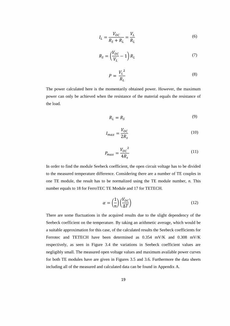
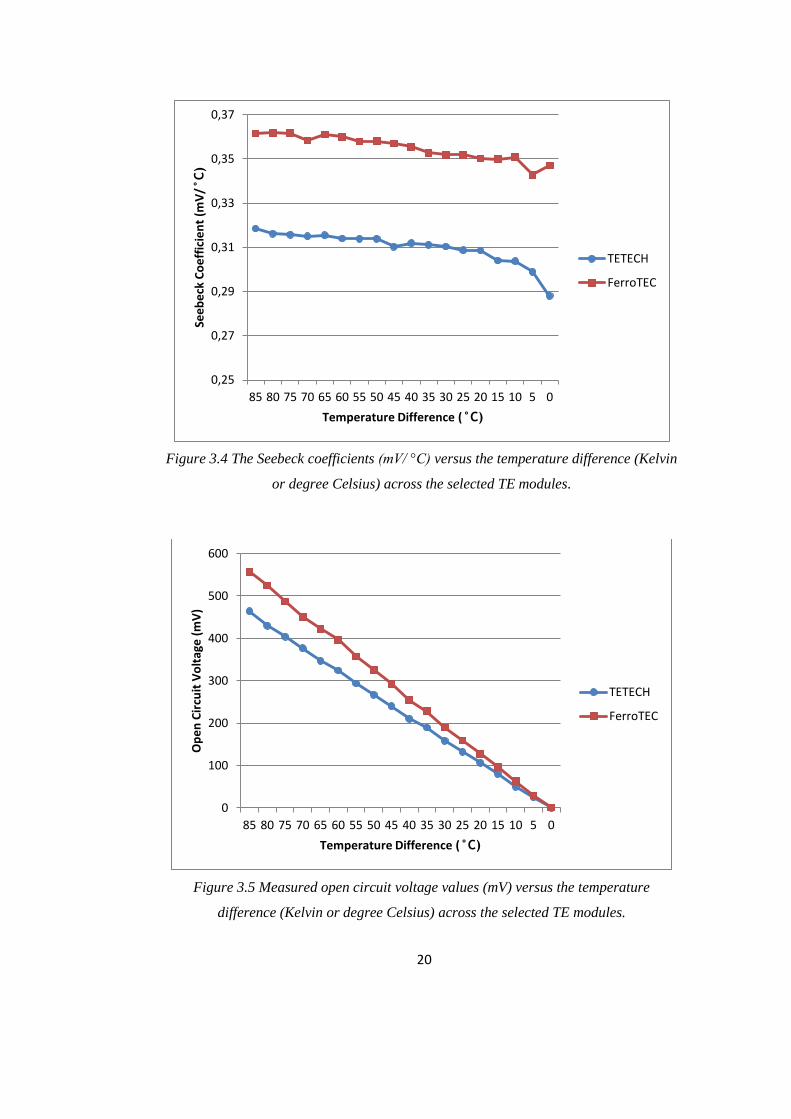
There are some fluctuations in the acquired results due to the slight dependency of the
Seebeck coefficient on the temperature. By taking an arithmetic average, which would be
a suitable approximation for this case, of the calculated results the Seebeck coefficients for
Ferrotec and TETECH have been determined as 0.354 mV/K and 0.308 mV/K
respectively, as seen in Figure 3.4 the variations in Seebeck coefficient values are
negligibly small. The measured open voltage values and maximum available power curves
for both TE modules have are given in Figures 3.5 and 3.6. Furthermore the data sheets
including all of the measured and calculated data can be found in Appendix A.
Page 35
20
Figure 3.4 The Seebeck coefficients (mV/ °C) versus the temperature difference (Kelvin
or degree Celsius) across the selected TE modules.
Figure 3.5 Measured open circuit voltage values (mV) versus the temperature
difference (Kelvin or degree Celsius) across the selected TE modules.
0,25
0,27
0,29
0,31
0,33
0,35
0,37
85 80 75 70 65 60 55 50 45 40 35 30 25 20 15 10 5 0
See
be
ck C
oe
ffic
ien
t (m
V/°
C)
Temperature Difference (°C)
TETECH
FerroTEC
0
100
200
300
400
500
600
85 80 75 70 65 60 55 50 45 40 35 30 25 20 15 10 5 0
Op
en
Cir
cuit
Vo
ltag
e (
mV
)
Temperature Difference (°C)
TETECH
FerroTEC
Page 36
21
Figure 3.6 Maximum power (milli-Watt) curves versus the temperature difference (Kelvin
or degree Celsius) across the selected TE modules.
0
5
10
15
20
25
30
35
85 80 75 70 65 60 55 50 45 40 35 30 25 20 15 10 5 0
Max
imu
m P
ow
er
(mW
)
Temperature Difference (°C)
FerroTEC
TETECH
Page 37
22
CHAPTER 4
MECHANICAL AND THERMAL CHARACTERIZATION OF THE
PLATFORMS
4.1 Selection and Basic Specifications of the Test Systems
By means of the recent advancements in the computer industry, the notebook usage
became quite widespread nowadays. In order to respond to different demands of users,
various new designs have been introduced, creating a wide variety of notebooks with
different sizes and features. Today the term “notebook” does not correspond to a single
object but a broad spectrum of designs, which vary in shape and mass. After consulting
the project sponsor Intel, it has been decided to select one notebook from each extreme
points of this spectrum to analyze in mechanical and thermal means. In this chapter the
analysis and the obtained data will be presented. However, at the end of the chapter only
one of the test systems will be selected for further investigation, and henceforth will be
referred as the target system.
The first test system Toshiba Portégé R705-P25 is an office type notebook that can easily
be transported around due to its light weighted design. Since it has a small and thin
geometry, this system can be classified as a “hot system” whose mechanical/thermal
design is relatively more complicated.
The second test system Dell Alienware M17xR2 has a large and heavy design. This
notebook is accepted as a leading gaming system due to its high performance. Its large
structure enables Alienware to operate in lower temperatures and it contains more reserve
space for alternative thermal and mechanical applications.
The basic specifications of each system have been presented in Figure 4.1, Table 4.1,
Figure 4.2 and Table 4.2.
Page 38
23
Toshiba Portégé R705-P25:
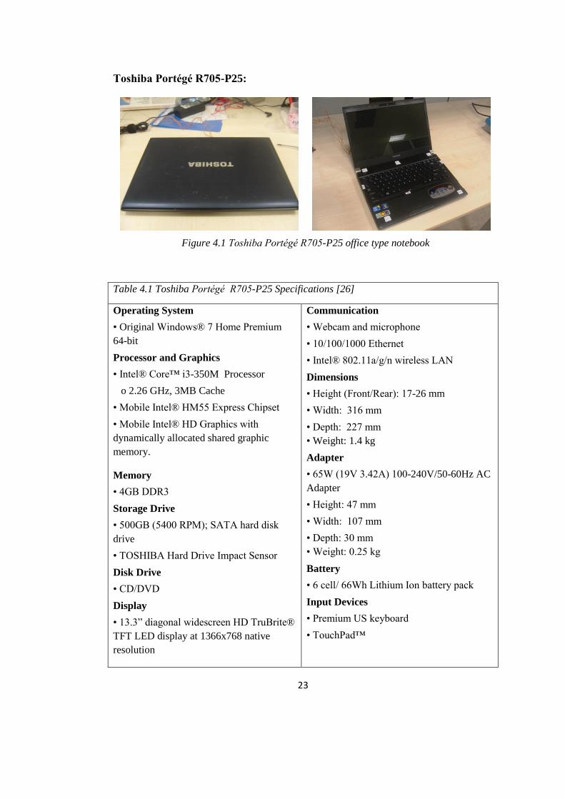
Figure 4.1 Toshiba Portégé R705-P25 office type notebook
Table 4.1 Toshiba Portégé R705-P25 Specifications [26]
Operating System
• Original Windows® 7 Home Premium
64-bit
Processor and Graphics
• Intel® Core™ i3-350M Processor
o 2.26 GHz, 3MB Cache
• Mobile Intel® HM55 Express Chipset
• Mobile Intel® HD Graphics with
dynamically allocated shared graphic
memory.
Memory
• 4GB DDR3
Storage Drive
• 500GB (5400 RPM); SATA hard disk
drive
• TOSHIBA Hard Drive Impact Sensor
Disk Drive
• CD/DVD
Display
• 13.3” diagonal widescreen HD TruBrite®
TFT LED display at 1366x768 native
resolution
Communication
• Webcam and microphone
• 10/100/1000 Ethernet
• Intel® 802.11a/g/n wireless LAN
Dimensions
• Height (Front/Rear): 17-26 mm
• Width: 316 mm
• Depth: 227 mm
• Weight: 1.4 kg
Adapter
• 65W (19V 3.42A) 100-240V/50-60Hz AC
Adapter
• Height: 47 mm
• Width: 107 mm
• Depth: 30 mm
• Weight: 0.25 kg
Battery
• 6 cell/ 66Wh Lithium Ion battery pack
Input Devices
• Premium US keyboard
• TouchPad™
Page 39
24
Dell Alienware M17xR2:
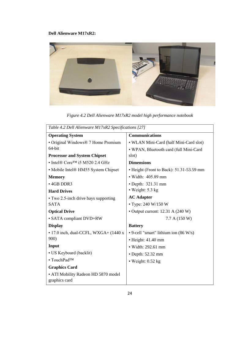
Figure 4.2 Dell Alienware M17xR2 model high performance notebook
Table 4.2 Dell Alienware M17xR2 Specifications [27]
Operating System
• Original Windows® 7 Home Premium
64-bit
Processor and System Chipset
• Intel® Core™ i5 M520 2.4 GHz
• Mobile Intel® HM55 System Chipset
Memory
• 4GB DDR3
Hard Drives
• Two 2.5-inch drive bays supporting
SATA
Optical Drive
• SATA compliant DVD+RW
Display
• 17.0 inch, dual-CCFL, WXGA+ (1440 x
900)
Input
• US Keyboard (backlit)
• TouchPad™
Graphics Card
• ATI Mobility Radeon HD 5870 model
graphics card
Communications
• WLAN Mini-Card (half Mini-Card slot)
• WPAN, Bluetooth card (full Mini-Card
slot)
Dimensions
• Height (Front to Back): 51.31-53.59 mm
• Width: 405.89 mm
• Depth: 321.31 mm
• Weight: 5.3 kg
AC Adapter
• Type: 240 W/150 W
• Output current: 12.31 A (240 W)
7.7 A (150 W)
Battery
• 9-cell "smart" lithium ion (86 W/s)
• Height: 41.40 mm
• Width: 292.61 mm
• Depth: 52.32 mm
• Weight: 0.52 kg
Page 40
25
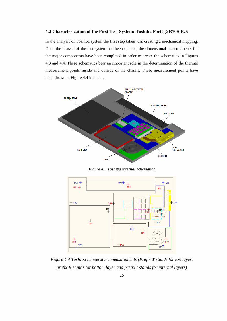
4.2 Characterization of the First Test System: Toshiba Portégé R705-P25
In the analysis of Toshiba system the first step taken was creating a mechanical mapping.
Once the chassis of the test system has been opened, the dimensional measurements for
the major components have been completed in order to create the schematics in Figures
4.3 and 4.4. These schematics bear an important role in the determination of the thermal
measurement points inside and outside of the chassis. These measurement points have
been shown in Figure 4.4 in detail.
Figure 4.3 Toshiba internal schematics
Figure 4.4 Toshiba temperature measurements (Prefix T stands for top layer,
prefix B stands for bottom layer and prefix I stands for internal layers)
Page 41
26
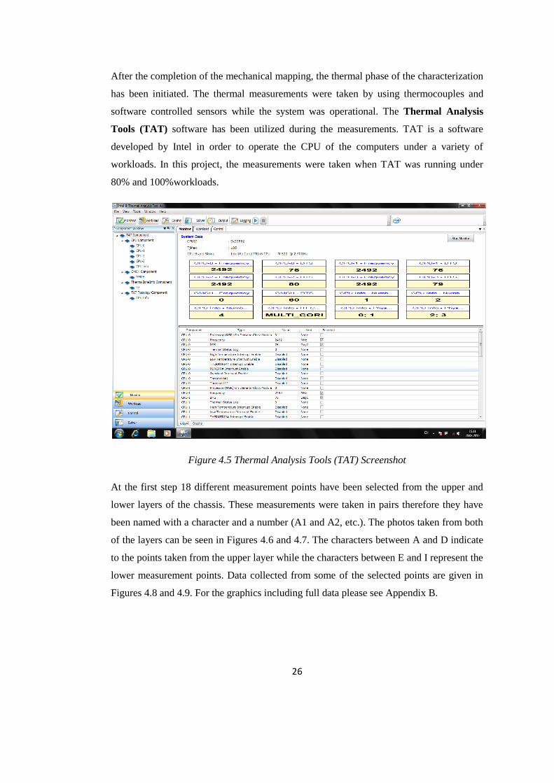
After the completion of the mechanical mapping, the thermal phase of the characterization
has been initiated. The thermal measurements were taken by using thermocouples and
software controlled sensors while the system was operational. The Thermal Analysis
Tools (TAT) software has been utilized during the measurements. TAT is a software
developed by Intel in order to operate the CPU of the computers under a variety of
workloads. In this project, the measurements were taken when TAT was running under
80% and 100%workloads.
Figure 4.5 Thermal Analysis Tools (TAT) Screenshot
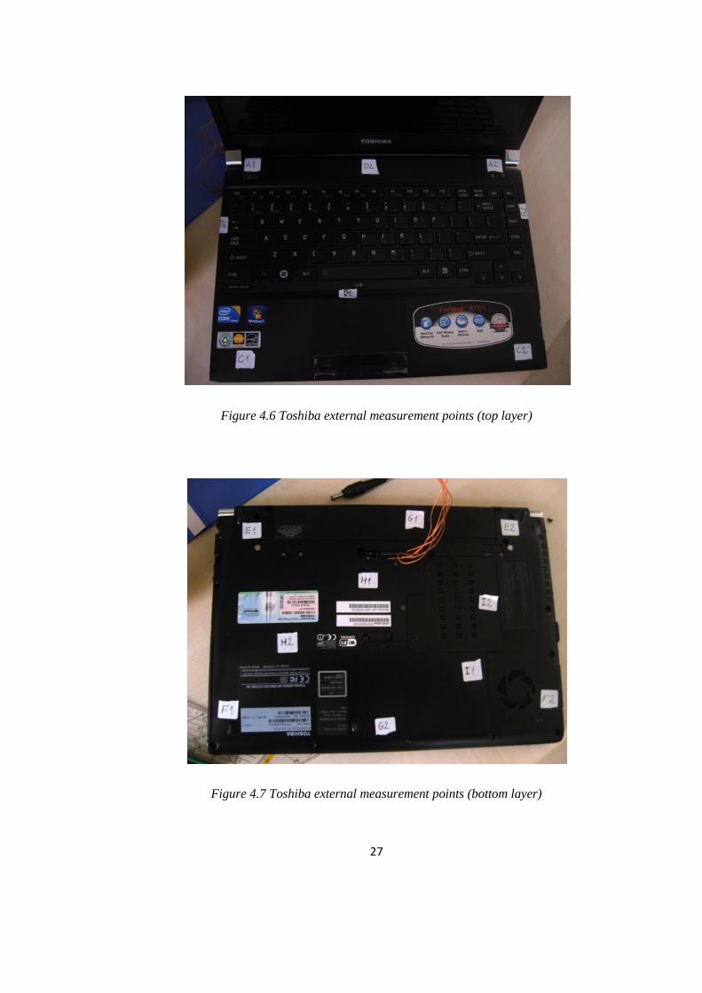
At the first step 18 different measurement points have been selected from the upper and
lower layers of the chassis. These measurements were taken in pairs therefore they have
been named with a character and a number (A1 and A2, etc.). The photos taken from both
of the layers can be seen in Figures 4.6 and 4.7. The characters between A and D indicate
to the points taken from the upper layer while the characters between E and I represent the
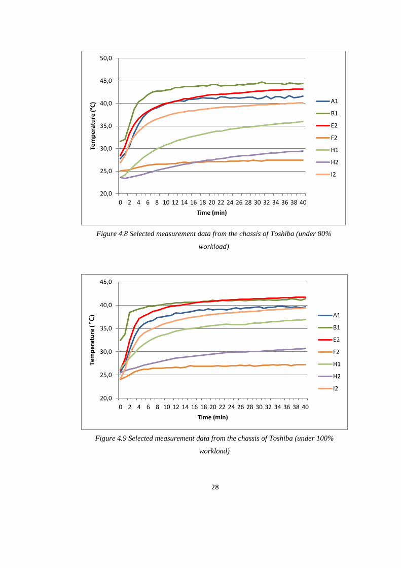
lower measurement points. Data collected from some of the selected points are given in
Figures 4.8 and 4.9. For the graphics including full data please see Appendix B.
Page 42
27
Figure 4.6 Toshiba external measurement points (top layer)
Figure 4.7 Toshiba external measurement points (bottom layer)
Page 43
28
Figure 4.8 Selected measurement data from the chassis of Toshiba (under 80%
workload)
Figure 4.9 Selected measurement data from the chassis of Toshiba (under 100%
workload)
20,0
25,0
30,0
35,0
40,0
45,0
50,0
0 2 4 6 8 10 12 14 16 18 20 22 24 26 28 30 32 34 36 38 40
Tem
pe
ratu
re (
°C)
Time (min)
A1
B1
E2
F2
H1
H2
I2
20,0
25,0
30,0
35,0
40,0
45,0
0 2 4 6 8 10 12 14 16 18 20 22 24 26 28 30 32 34 36 38 40
Tem
pe
ratu
re (°C)
Time (min)
A1
B1
E2
F2
H1
H2
I2
Page 44
29
The charts in Figures 4.8 and 4.9 show two important results:
The temperature distribution on different parts of the chassis varies between the
ambient temperature (≈ 25°C )and 45°C while the system is operational.
The system obtains larger temperature values while operating under 80%
workload. This result is an outcome of the fan efficiency. It has been observed
that the fan of the notebook runs faster under 100% workload, thus creating a
stronger air flow to cool down the system.
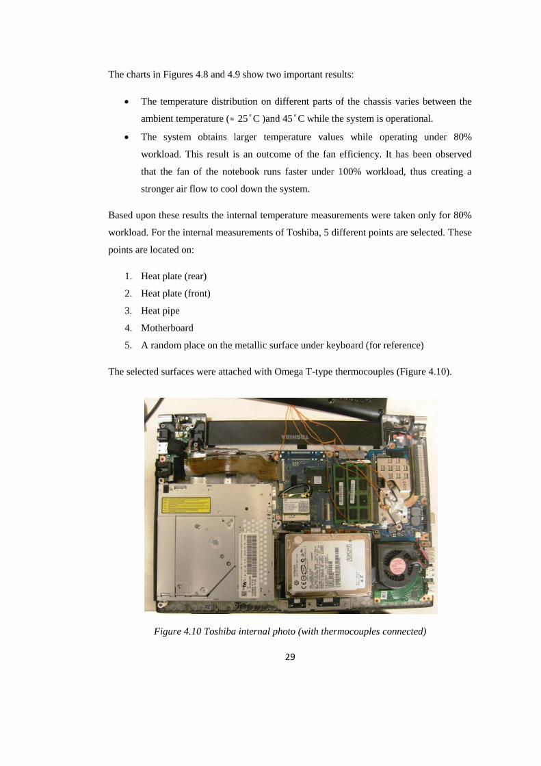
Based upon these results the internal temperature measurements were taken only for 80%
workload. For the internal measurements of Toshiba, 5 different points are selected. These
points are located on:
1. Heat plate (rear)
2. Heat plate (front)
3. Heat pipe
4. Motherboard
5. A random place on the metallic surface under keyboard (for reference)
The selected surfaces were attached with Omega T-type thermocouples (Figure 4.10).
Figure 4.10 Toshiba internal photo (with thermocouples connected)
Page 45
30
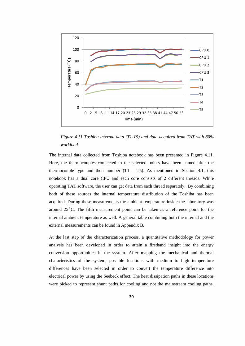
Figure 4.11 Toshiba internal data (T1-T5) and data acquired from TAT with 80%
workload.
The internal data collected from Toshiba notebook has been presented in Figure 4.11.
Here, the thermocouples connected to the selected points have been named after the
thermocouple type and their number (T1 – T5). As mentioned in Section 4.1, this
notebook has a dual core CPU and each core consists of 2 different threads. While
operating TAT software, the user can get data from each thread separately. By combining
both of these sources the internal temperature distribution of the Toshiba has been
acquired. During these measurements the ambient temperature inside the laboratory was
around 25°C. The fifth measurement point can be taken as a reference point for the
internal ambient temperature as well. A general table combining both the internal and the
external measurements can be found in Appendix B.
At the last step of the characterization process, a quantitative methodology for power
analysis has been developed in order to attain a firsthand insight into the energy
conversion opportunities in the system. After mapping the mechanical and thermal
characteristics of the system, possible locations with medium to high temperature
differences have been selected in order to convert the temperature difference into
electrical power by using the Seebeck effect. The heat dissipation paths in these locations
were picked to represent shunt paths for cooling and not the mainstream cooling paths.
0
20
40
60
80
100
120
0 2 5 8 11 14 17 20 23 26 29 32 35 38 41 44 47 50 53
Tem
pe
ratı
re (°C)
Time (min)
CPU 0
CPU 1
CPU 2
CPU 3
T1
T2
T3
T4
T5
Page 46
31
This method has been followed on purpose to avoid significant performance impact. The
maximum power generation potential has been calculated by using the maximum power
curve for both of the TE modules, which were presented in Figure 3.4. During these
calculations, it has been assumed that the temperature differences between the selected
points are constant and available for the geometrical space between the points. Also
instead of placing a standard TE module, which has surface dimensions of 6.3 mm x 6.3
mm for TETECH and 6.05 mm x 6.05 mm for FerroTEC, the whole area given for each
location was assumed to be filled with TE couples. In the end the results were summed up
and a power discount of 50% has been applied to the end result in order to represent
possible power losses.
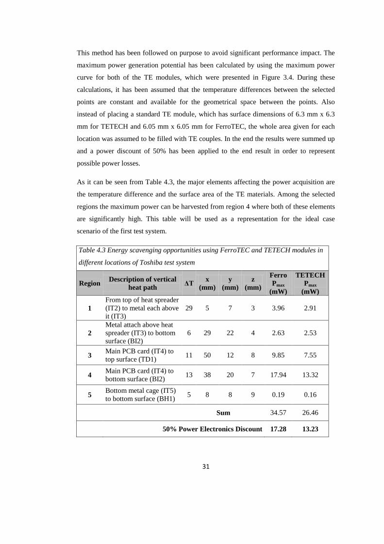
As it can be seen from Table 4.3, the major elements affecting the power acquisition are
the temperature difference and the surface area of the TE materials. Among the selected
regions the maximum power can be harvested from region 4 where both of these elements
are significantly high. This table will be used as a representation for the ideal case
scenario of the first test system.
Table 4.3 Energy scavenging opportunities using FerroTEC and TETECH modules in
different locations of Toshiba test system
Region Description of vertical
heat path ΔT
x
(mm)
y
(mm)
z
(mm)
Ferro
Pmax
(mW)
TETECH
Pmax
(mW)
1
From top of heat spreader
(IT2) to metal each above
it (IT3)
29 5 7 3 3.96 2.91
2
Metal attach above heat
spreader (IT3) to bottom
surface (BI2)
6 29 22 4 2.63 2.53
3 Main PCB card (IT4) to
top surface (TD1) 11 50 12 8 9.85 7.55
4 Main PCB card (IT4) to
bottom surface (BI2) 13 38 20 7 17.94 13.32
5 Bottom metal cage (IT5)
to bottom surface (BH1) 5 8 8 9 0.19 0.16
Sum 34.57 26.46
50% Power Electronics Discount 17.28 13.23
Page 47
32
4.3 Characterization of the Second Test System: Dell Alienware M17xR2
In this section the second test system, Alienware, is examined. There are some major
differences between Alienware and Toshiba and some of these differences will also be
reflected to the experimentation procedure. First of all Alienware has a much bigger
geometry in comparison to Toshiba and has very good thermal insulation on its outer
chassis, which renders the external temperature measurements unimportant. Therefore the
experimental procedure of AW will directly start with interior mechanical mapping.
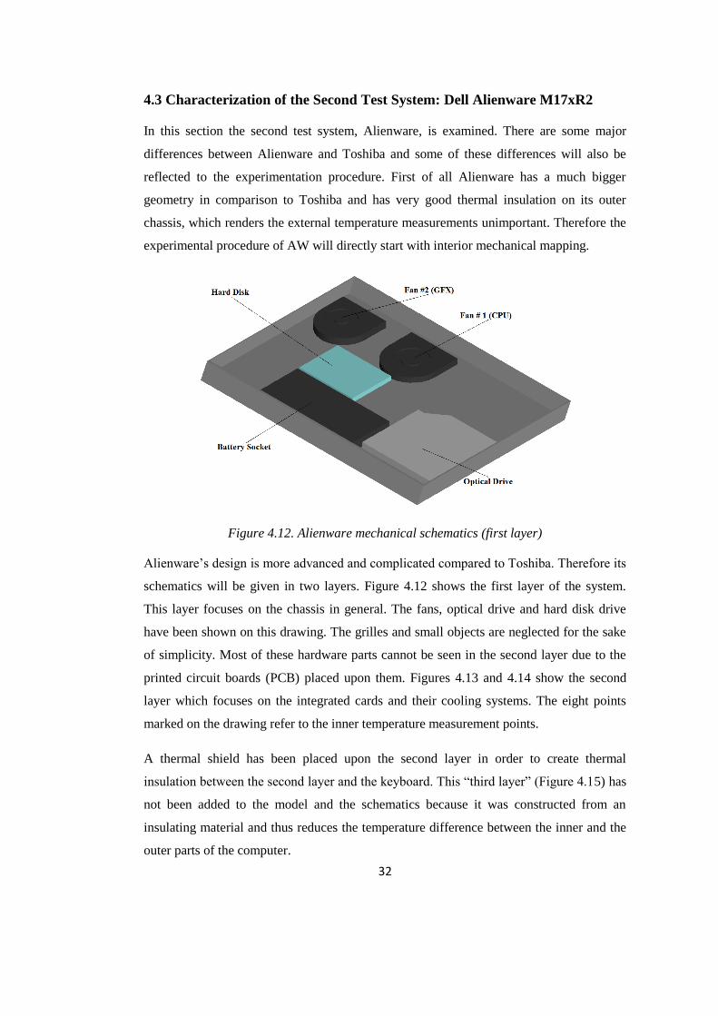
Figure 4.12. Alienware mechanical schematics (first layer)
Alienware’s design is more advanced and complicated compared to Toshiba. Therefore its
schematics will be given in two layers. Figure 4.12 shows the first layer of the system.
This layer focuses on the chassis in general. The fans, optical drive and hard disk drive
have been shown on this drawing. The grilles and small objects are neglected for the sake
of simplicity. Most of these hardware parts cannot be seen in the second layer due to the
printed circuit boards (PCB) placed upon them. Figures 4.13 and 4.14 show the second
layer which focuses on the integrated cards and their cooling systems. The eight points
marked on the drawing refer to the inner temperature measurement points.
A thermal shield has been placed upon the second layer in order to create thermal
insulation between the second layer and the keyboard. This “third layer” (Figure 4.15) has
not been added to the model and the schematics because it was constructed from an
insulating material and thus reduces the temperature difference between the inner and the
outer parts of the computer.
Page 48
33
Figure 4.13 Alienware mechanical schematics (second layer) and the thermal
measurement points
Figure 4.14 Alienware, photo of the second layer (graphics card removed)
Page 49
34
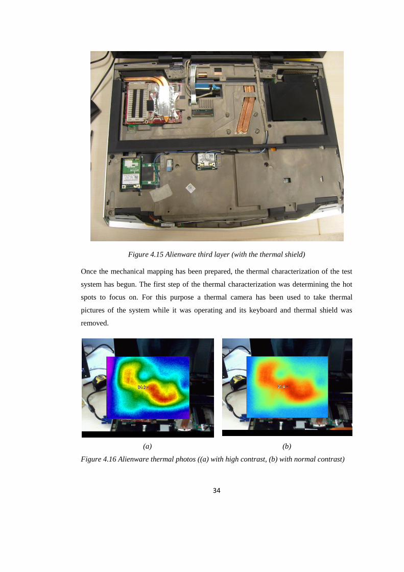
Figure 4.15 Alienware third layer (with the thermal shield)
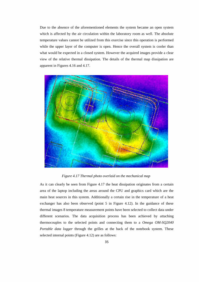
Once the mechanical mapping has been prepared, the thermal characterization of the test
system has begun. The first step of the thermal characterization was determining the hot
spots to focus on. For this purpose a thermal camera has been used to take thermal
pictures of the system while it was operating and its keyboard and thermal shield was
removed.
(a) (b)
Figure 4.16 Alienware thermal photos ((a) with high contrast, (b) with normal contrast)
Page 50
35
Due to the absence of the aforementioned elements the system became an open system
which is affected by the air circulation within the laboratory room as well. The absolute
temperature values cannot be utilized from this exercise since this operation is performed
while the upper layer of the computer is open. Hence the overall system is cooler than
what would be expected in a closed system. However the acquired images provide a clear
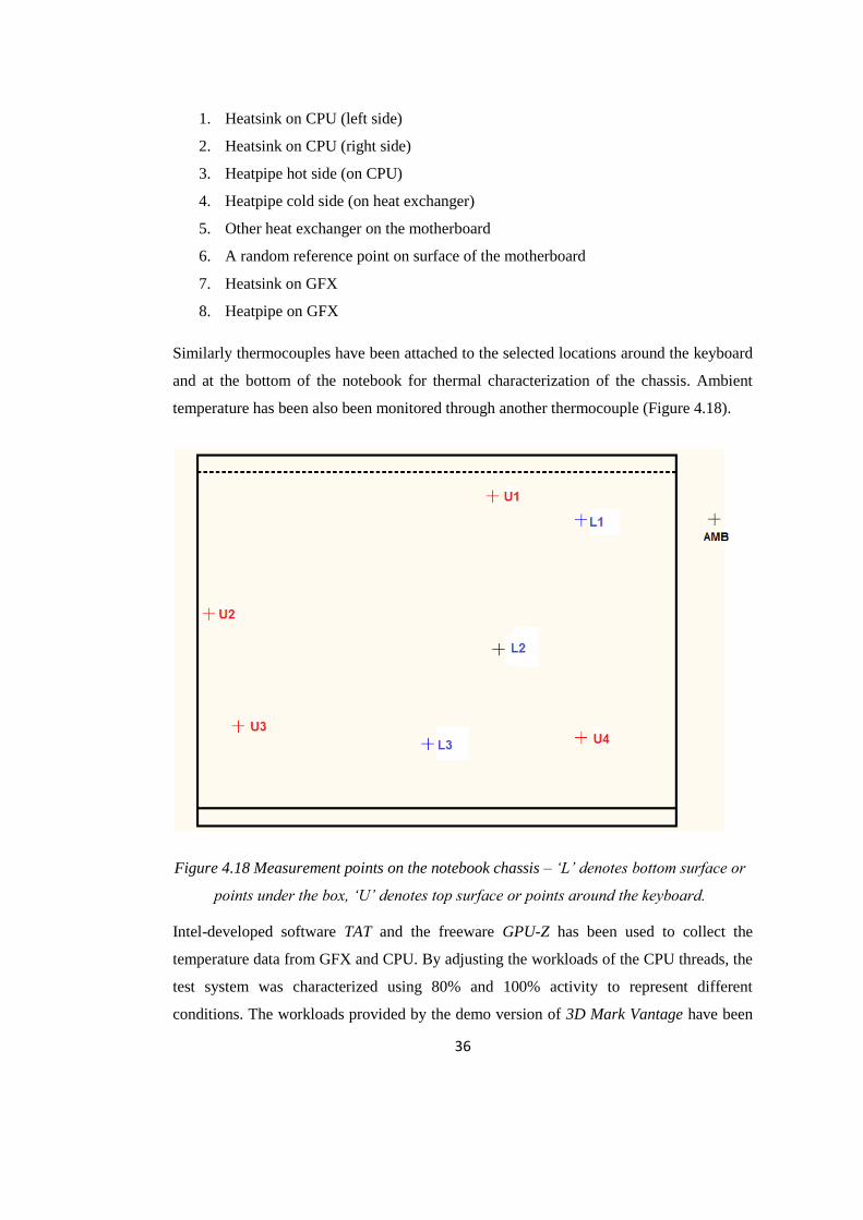
view of the relative thermal dissipation. The details of the thermal map dissipation are
apparent in Figures 4.16 and 4.17.
Figure 4.17 Thermal photo overlaid on the mechanical map
As it can clearly be seen from Figure 4.17 the heat dissipation originates from a certain
area of the laptop including the areas around the CPU and graphics card which are the
main heat sources in this system. Additionally a certain rise in the temperature of a heat
exchanger has also been observed (point 5 in Figure 4.12). In the guidance of these
thermal images 8 temperature measurement points have been selected to collect data under
different scenarios. The data acquisition process has been achieved by attaching
thermocouples to the selected points and connecting them to a Omega OM-SQ2040
Portable data logger through the grilles at the back of the notebook system. These
selected internal points (Figure 4.12) are as follows:
Page 51
36
1. Heatsink on CPU (left side)
2. Heatsink on CPU (right side)
3. Heatpipe hot side (on CPU)
4. Heatpipe cold side (on heat exchanger)
5. Other heat exchanger on the motherboard
6. A random reference point on surface of the motherboard
7. Heatsink on GFX
8. Heatpipe on GFX
Similarly thermocouples have been attached to the selected locations around the keyboard
and at the bottom of the notebook for thermal characterization of the chassis. Ambient
temperature has been also been monitored through another thermocouple (Figure 4.18).
Figure 4.18 Measurement points on the notebook chassis – ‘L’ denotes bottom surface or
points under the box, ‘U’ denotes top surface or points around the keyboard.
Intel-developed software TAT and the freeware GPU-Z has been used to collect the
temperature data from GFX and CPU. By adjusting the workloads of the CPU threads, the
test system was characterized using 80% and 100% activity to represent different
conditions. The workloads provided by the demo version of 3D Mark Vantage have been
Page 52
37
operated to exercise graphics during the experimentation which consists of two
independent animations:
1. Jane Nash (lasts 1:40 min) is an animation focusing on the details of the large
objects. The number of the objects is relatively low while their geometries are
bigger and more detailed.
2. New Calico (lasts 2:40 min) has a lot of small objects. The detail of the objects
are lower than the previous animation, however the number of independent
objects are rather high.
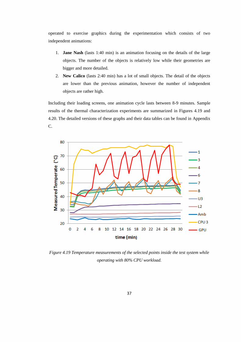
Including their loading screens, one animation cycle lasts between 8-9 minutes. Sample
results of the thermal characterization experiments are summarized in Figures 4.19 and
4.20. The detailed versions of these graphs and their data tables can be found in Appendix
C.
Figure 4.19 Temperature measurements of the selected points inside the test system while
operating with 80% CPU workload.
Page 53
38
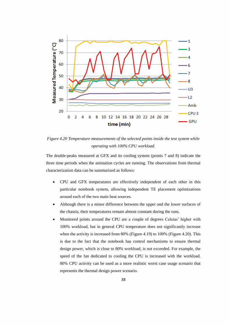
Figure 4.20 Temperature measurements of the selected points inside the test system while
operating with 100% CPU workload.
The double-peaks measured at GFX and its cooling system (points 7 and 8) indicate the
three time periods when the animation cycles are running. The observations from thermal
characterization data can be summarized as follows:
CPU and GFX temperatures are effectively independent of each other in this
particular notebook system, allowing independent TE placement optimizations
around each of the two main heat sources.
Although there is a minor difference between the upper and the lower surfaces of
the chassis, their temperatures remain almost constant during the runs.
Monitored points around the CPU are a couple of degrees Celsius’ higher with
100% workload, but in general CPU temperature does not significantly increase
when the activity is increased from 80% (Figure 4.19) to 100% (Figure 4.20). This
is due to the fact that the notebook has control mechanisms to ensure thermal
design power, which is close to 80% workload, is not exceeded. For example, the
speed of the fan dedicated to cooling the CPU is increased with the workload.
80% CPU activity can be used as a more realistic worst case usage scenario that
represents the thermal design power scenario.
Page 54
39
The maximum operating condition for the CPU is specified as 105°C [28] in the
datasheet. Yet the temperature is regulated to stay under 82°C in this notebook.
This approach potentially leaves headroom in the platform for TE integration
closer to CPU. This additional temperature margin will not be utilized in this
thesis, since its main approach is addressing the tougher case of a thermally
limited system.
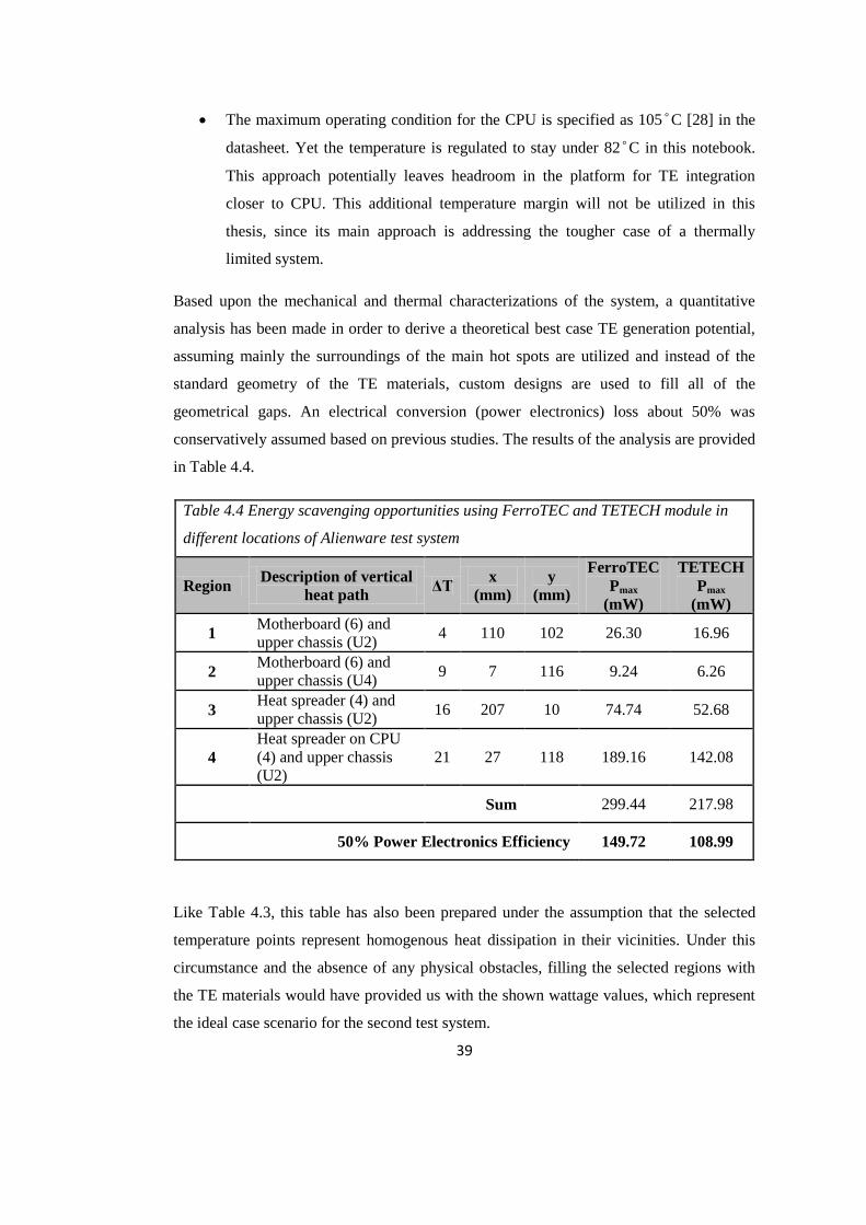
Based upon the mechanical and thermal characterizations of the system, a quantitative
analysis has been made in order to derive a theoretical best case TE generation potential,
assuming mainly the surroundings of the main hot spots are utilized and instead of the
standard geometry of the TE materials, custom designs are used to fill all of the
geometrical gaps. An electrical conversion (power electronics) loss about 50% was
conservatively assumed based on previous studies. The results of the analysis are provided
in Table 4.4.
Table 4.4 Energy scavenging opportunities using FerroTEC and TETECH module in
different locations of Alienware test system
Region Description of vertical
heat path ΔT
x
(mm)
y
(mm)
FerroTEC
Pmax
(mW)
TETECH
Pmax
(mW)
1 Motherboard (6) and
upper chassis (U2) 4 110 102 26.30 16.96
2 Motherboard (6) and
upper chassis (U4) 9 7 116 9.24 6.26
3 Heat spreader (4) and
upper chassis (U2) 16 207 10 74.74 52.68
4
Heat spreader on CPU
(4) and upper chassis
(U2)
21 27 118 189.16 142.08
Sum 299.44 217.98
50% Power Electronics Efficiency 149.72 108.99
Like Table 4.3, this table has also been prepared under the assumption that the selected
temperature points represent homogenous heat dissipation in their vicinities. Under this
circumstance and the absence of any physical obstacles, filling the selected regions with
the TE materials would have provided us with the shown wattage values, which represent
the ideal case scenario for the second test system.
Page 55
40
4.4 Selection of the Target System
In this chapter both of the test systems have been analyzed on thermal, mechanical and
power production basis. Although the thermal conditions of Toshiba system seem better at
the first glance, Alienware has a much larger chassis enabling a larger amount of TE
integration possibilities, which affects the quantitative power production model as well.
By comparing Tables 4.3 and 4.4, it can be clearly seen that Alienware is much more
advantageous in the power production branch. Since it is not classified as a hot system, the
danger of overheating or heat related performance losses are also more difficult to occur in
comparison to the Toshiba system. In conclusion Dell Alienware M17xR2 has been
selected as the target system of this thesis. For a more detailed study, computer
simulations of its major parts and the whole system will be made in the following
chapters.
4.5 Effects of the TE Module Integration on the Carbon Footprints
A small model may be helpful to estimate the environmental effects of the TE module
integration on the notebook computers. Based upon the results shown in Table 4.4, it may
be assumed that a TE integrated notebook computer would require 0.15 Whr less energy
per hour. (The size variations among different notebook computer models have been
neglected.) The researches show that there were around 1.2 billion mobile computers in
the world in 2008 [29]. It is estimated that the number will be 2 billion by around 2015. If
all of these computers would have TE modules integrated inside them, providing an
energy of 0.15 Whr in each, this would decrease the hourly energy need by an amount of:
(13)
In a thermic power plant around 250 g of oil needs to be consumed to produce 1 kWhr
electricity [30].
(14)
It follows that global TE integration in computers would create a decrease of 75 tons of oil
consumption per hour by year 2015. This would correspond to a yearly drop of 657,000
tons in the oil consumption. In order to calculate the carbon footprint of this amount, the
stoichiometric equation of the fuel burning must be taken into consideration:
Page 56
41
(15)
Equation (15) indicates that 108 g fuel exhausts 352 g CO2 while burning.
(16)
This simple model presents that globalizing the TE module integration would cause a drop
of nearly 2 million tons of annual CO2 dissipation by year 2015. The model ignores the
CO2 emissions during the manufacturing and distribution or transportation of the TE
modules. It also ignores the transmission, distribution, and conversion electricity losses
from the thermic power station to the computer load. On the other hand, the result is
sufficient to demonstrate that every mW saving counts when it comes to one of the fastest
growing industries.
Page 57
42
CHAPTER 5
TARGET SYSTEM MODELING
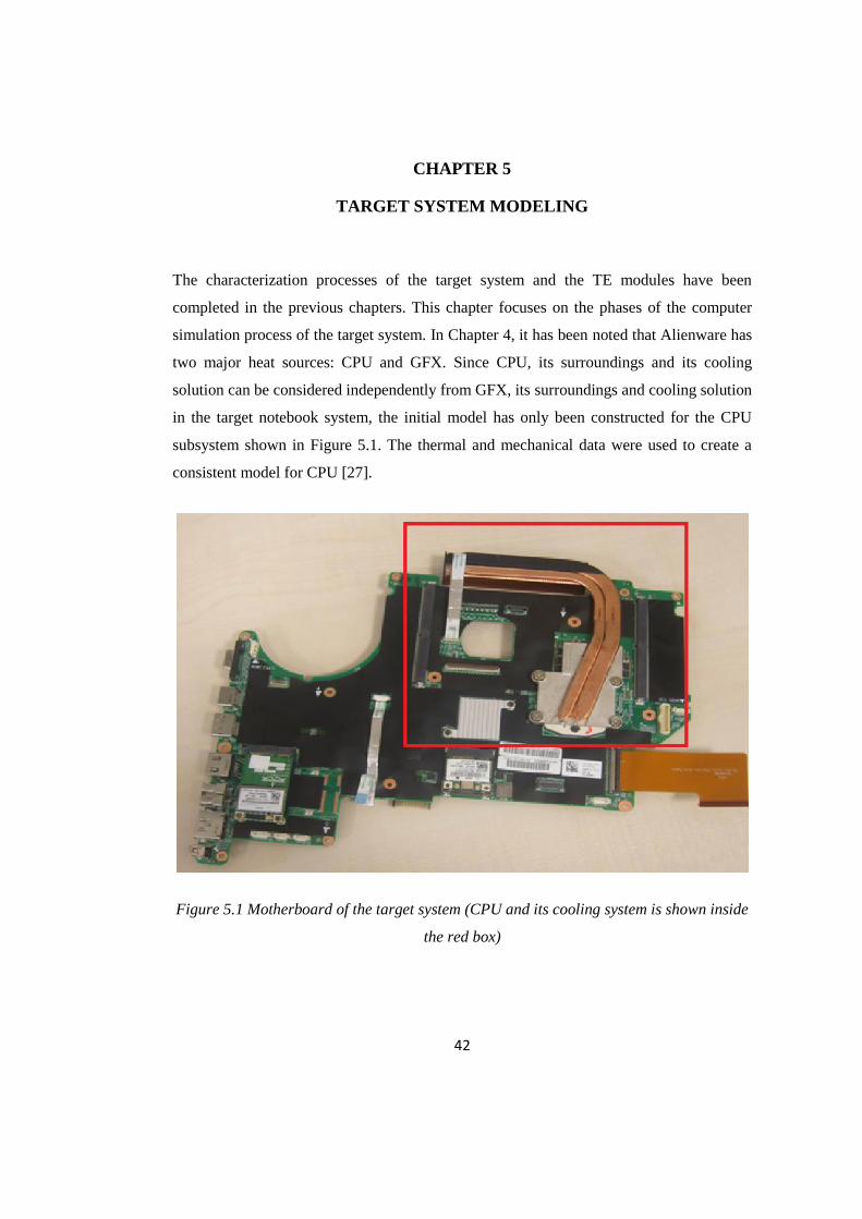
The characterization processes of the target system and the TE modules have been
completed in the previous chapters. This chapter focuses on the phases of the computer
simulation process of the target system. In Chapter 4, it has been noted that Alienware has
two major heat sources: CPU and GFX. Since CPU, its surroundings and its cooling
solution can be considered independently from GFX, its surroundings and cooling solution
in the target notebook system, the initial model has only been constructed for the CPU
subsystem shown in Figure 5.1. The thermal and mechanical data were used to create a
consistent model for CPU [27].
Figure 5.1 Motherboard of the target system (CPU and its cooling system is shown inside
the red box)
Page 58
43
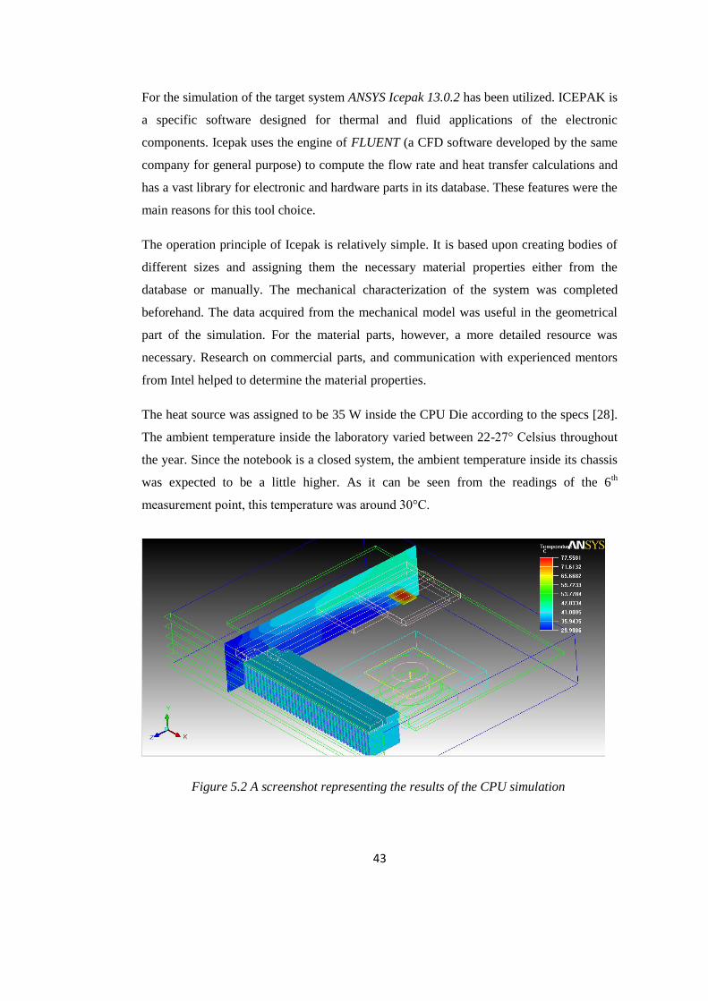
For the simulation of the target system ANSYS Icepak 13.0.2 has been utilized. ICEPAK is
a specific software designed for thermal and fluid applications of the electronic
components. Icepak uses the engine of FLUENT (a CFD software developed by the same
company for general purpose) to compute the flow rate and heat transfer calculations and
has a vast library for electronic and hardware parts in its database. These features were the
main reasons for this tool choice.
The operation principle of Icepak is relatively simple. It is based upon creating bodies of
different sizes and assigning them the necessary material properties either from the
database or manually. The mechanical characterization of the system was completed
beforehand. The data acquired from the mechanical model was useful in the geometrical
part of the simulation. For the material parts, however, a more detailed resource was
necessary. Research on commercial parts, and communication with experienced mentors
from Intel helped to determine the material properties.
The heat source was assigned to be 35 W inside the CPU Die according to the specs [28].
The ambient temperature inside the laboratory varied between 22-27° Celsius throughout
the year. Since the notebook is a closed system, the ambient temperature inside its chassis
was expected to be a little higher. As it can be seen from the readings of the 6th
measurement point, this temperature was around 30°C.
Figure 5.2 A screenshot representing the results of the CPU simulation
Page 59
44
Figure 5.3 Utilized mesh control settings of Icepak
Once the simulation is completed, Icepak presents a solution overview file with numerical
results. It is also possible to have a visual presentation of results for temperature
distribution in a contour map or for the air flow in a colored vector field. Such a
presentation of temperature distribution is depicted in Figure 5.2. In this simulation all of
the heat transfer modes (conduction, convection and radiation) were enabled, while the
ambient temperature was set to 30°C. The details of the meshing settings can be seen in
Figure 5.3.
Table 5.1 Measured and simulated values for CPU simulation
Measured Simulated (Max. Temp.)
Microprocessor
CPU-0 72 °C
79.0 °C CPU-1 71 °C
CPU-2 79 °C
CPU-3 79 °C
Heat Sink 1 48.3 °C
49.2 – 51.9°C 2 48.3 °C
Heat Pipes and
HEX
3 46.4 °C 49.7 °C
4 47.6 °C 48.7 °C
PCB 6 35.5 °C 31.5 °C
Page 60
45
Also a small comparison between the numerical values and the measurements is provided
in Table 5.1. As shown in the table, the initial results are very close to the measured values
and the minor differences are within the limits of tolerance. Henceforth the first version of
the simulation was accepted to be successful. This simulation and its values will be
utilized in the next chapter for the selection of a plausible location for the TE module.
Although this version of the simulation was successful, it only covers geometrically 1/6 of
the whole system and excludes a secondary thermal source, the GFX area, which has a
certain (small) degree of thermal interdependency with CPU. Since the aim of this thesis
was to create a model for the whole system the simulation was upgraded several times.
The most important step was creating the simulation of the GFX area and merging it with
the CPU simulation.
Figure 5.4 ATI Mobility Radeon HD 5870 model graphics card
The first problem about the simulation of the GFX was determining the wattage of the
graphics card. Generally the graphics cards would be motherboard integrated in the
notebooks and carry a small about of wattage. However Alienware is a specifically gamer
oriented notebook. Therefore it has an independent ATI Mobility Radeon HD 5870 model
graphics card with a separate cooling solution including a fan, a heatsink, a couple of
heatpipes and two separate heat exchangers as seen in Figure 5.4.
Page 61
46
It is difficult to say the exact wattage of this graphics card; however it has been stated in a
semi-official source to be around 50 W [31]. There is another important point which has a
mild impact on the results. As stated in the previous chapters the measurement period for
the GFX is based upon the demo version of 3D Mark Vantage. Unlike its counterpart in
CPU measurements, 3D Mark only remains operational for a short amount of time and
keeps repeating the same cycle. Thus the graphics card of the system can reach neither its
maximum condition, nor steady state as shown in Figures 4.19 and 4.20. Unfortunately the
power sources in Icepak cannot be adjusted to be time dependent. A power source can be
either constant or temperature dependent. Since the power measurements of GFX are out
of the scope of this thesis, the first option has been selected, fixing the power of GFX at
50 W. Therefore the results involving the measurement points on the graphics card would
be higher than the collected data, representing a semi-realistic scenario where the GFX
reaches its maximum value and remains at a steady state.
Figure 5.5 A screenshot from the simulation of GFX
After the merger of the simulations of CPU and GFX, the last step for completing the
simulation was increasing the cabinet size to the size of the chassis and placing additional
bodies representing major objects shown in the schematics (Figure 4.13). Table 5.2 has
been prepared for the comparison of the measured and simulated data. The actual
Page 62
47
overview and a detailed version of the simulation report are placed in Appendix E. A
screenshot from Full Simulation without TE can be seen in Figure 5.6.
Table 5.2 Measured and simulated values for the whole simulation (in °C)
Measured Simulated (Max. Temp.)
Microprocessor
CPU-0 73
78.4 CPU-1 71
CPU-2 79
CPU-3 78
Heat Sink on CPU 1 48.2
46.5-51.6 2 48.2
Hear Pipes and HEX on
CPU
3 46.4 46.6
4 47.5 45.9
HEX on the motherboard 5 40.7 43.7
PCB 6 35.4 31.3
Heatsink on GFX 7 44.7 56.6
Heatpipe on GFX 8 46.8 56.5
GFX Source GPU 72 77.2
Figure 5.6 A screenshot from the Final Simulation without TE
Page 63
48
CHAPTER 6
THERMOELECTRIC MODULE INTEGRATION ANALYSIS AND
VALIDATION
This chapter is split into four sections. The first section describes the simulations
performed for selecting a feasible location for the TE module. In the second section, the
TE module is physically attached to the selected coordinates in the actual target system,
and thermal impact of the TE module on the system is characterized. The results obtained
from TE integration is compared to the simulation predictions in the third section. The last
section discusses results, and power production possibilities based on physical validation
experiments.
6.1 Selecting a Feasible Integration Point for TE Module
The selection of a correct spot is an important, but also difficult step of this project.
Because the selected spot needs to be close to the heat source in order to harvest enough
heat to create a plausible amount of temperature difference between the surfaces of the TE
module. But picking a shunt path location that has a minimum or no impact to the CPU
temperature in order to preserve performance is also essential. As stated previously there
are only two major heat sources in the target system. Since the CPU is more consistent
than GFX, the selection process will be carried out within the CPU simulation.
The first steps of the selection procedure are methodologically empirical. Therefore only
some of the preliminary selections will be presented (Figure 6.1). At the first step a small
model of the TE module has been prepared and has been placed:
1. On CPU die (red)
2. Inside the heat sink (blue)
3. Under the heat sink (green)
4. On top of the heat spreader (purple)
5. On top of the heat exchanger (grey)
6. Under the heat pipe (yellow)
Page 64
49
Figure 6.1 The locations of the preliminarily selected points for TE module
Table 6.1 Integration results in the simulation
Ref. 1 2 3 4 5 6
Coordinates (mm)
x - 0 0 0 15 50 0
y - 0 0.2 -2.7 3.2 8.5 0.3
z - 0 15 30 0 91 60
Power Source (°C) CPU_Source 79.0 100.2 74.6 78.3 85.7 84.9 76.3
Heat Sink (°C) CPU_Block 51.9 63.5 47.5 51.3 58.2 57.9 49.2
CPU_Block.1 49.2 49.8 44.8 48.5 55.4 55.2 46.5
Heat Pipes (°C)
block.1 49.1 49.8 44.7 48.4 55.3 55.1 46.3
block.2 49.7 50.2 45.2 49.0 55.9 55.7 46.9
block.3 48.7 49.3 44.3 48.0 54.9 54.7 46.0
block.4 48.7 49.3 44.3 48.0 54.9 54.7 45.9
BGA (°C) BGA 52.6 55.9 49.4 52.0 57.3 57.1 50.7
Die (°C) Die 78.9 100.2 74.5 78.2 85.6 84.8 76.2
Sockets and pins (°C) Socket and
Pins 53.7 57.3 50.3 53.0 58.6 58.2 51.6
Thermoelectric Module (°C)
BiTe.1 - 88.9 44.9 48.0 54.5 52.5 46.2
TE bottom.1 - 89.9 44.9 36.4 54.5 52.6 33.8
TE top.1 - 51.7 44.9 48.4 43.4 34.4 46.2
Temperature
Difference - 38.2 0.04 12.0 11.2 18.1 12.3
Page 65
50
The temperature difference between the faces of the TE model has been taken as the
primary parameter in these attempts. Table 6.1 shows the data obtained from these
simulations. In order to create a geometrical understanding, the first spot, which has been
selected exactly on the CPU die, has been set as the origin and the other locations have
been given coordinates relatively. Also a reference column has been given in order to
highlight the heating or performance effects of the integration attempts on the system.
This initial integration attempts provided essential information about possible effects of
the TE integration on different spots around CPU. However none of the above selections
qualify as a correct selection. Capturing a decent temperature difference may have been
the initial purpose; however any selection triggering an overheating may cause the system
performance loss. Therefore points 1, 4 and 5 have been eliminated at the first step.
Among the others the factor of physical obstacles kicks in, because there is a thermal
shield on the actual system rendering most selections like point 6 impossible and points
like 2 and 3 need some machining work in order to be integrated which may be harmful to
the cooling solution or create short circuits in the PCB area.
Figure 6.2 The virtual results of the TE integration on the 7th point. (TE module has been
highlighted in the red circle)
All those reasons considered, a seventh point has been selected as the appropriate spot for
the TE integration which has been close to the 1st point in the previous attempts. A slight
relocation in the assigned coordinate system (0; 0; 8.1) has enabled the TE module to fit
into a gap on the thermal shield (Figure 6.3). Also the TE module has been placed on one
of the heat pipes instead of the CPU Die to overcome the heating problem. Therefore the
Page 66
51
seventh point has been selected to be the integration point for the TE module. The results
of the CPU simulation including the TE module have been given in Figure 6.2 and Table
6.2.
Table 6.2 A comparison for the results obtained before and after the TE integration
on point 7
Temperature results without TE
integration
Temperature results for 7th
point
Measured
Simulated
(Max. Temp.) Measured
Simulated
(Max. Temp.)
Microprocessor
CPU-0 72
79.0
CPU-0 72
76.1 CPU-1 71 CPU-1 73
CPU-2 79 CPU-2 79
CPU-3 79 CPU-3 79
Heat Sink 1 48.3
49.2 - 51.9 1 47.9
45.7 - 48.6 2 48.3 2 47.9
Heat Pipes and
HEX
3 46.4 49.7 3 47.0 45.6
4 47.6 48.7 4 47.3 45.3
TE lower surface
- - 48.7 41.4
TE upper surface
- - 40.3 29.1
Figure 6.3 The TE integration on the actual system (with the keyboard removed)
Page 67
52
As it can clearly be seen from these results, the selected point does not create any
unrequited heat loads and also it seems to have discharged some of the heat around to
CPU area creating a minor cooling effect. This cooling may be more apparent in the
simulations due to the idealized conditions and the minor temperature drop in the
measured data might have been caused by externalities as well. Yet the data exhibited in
this table proves that implementing the TE module on this point composes no danger of
overheating in the system..
6.2 TE Module Integration and Analysis
The integration process has begun after selecting a suitable spot for TE module. Due to its
higher efficiency the TE module of FerroTEC has been selected to be used in application
parts. Most of the thermocouples have been preserved from the system characterization in
Chapter 4. Yet due to the number limitations in the data logger two of the exterior
thermocouples (U1 and U2 from Figure 4.18) had to be replaced and attached to the both
sides of TE module in order to observe the temperature differences as well. A thermal
paste has been put between the selected spot (Figure 6.3) and the lower surface of the TE
module, in order to reduce the contact resistance. Due to the unavailability of any
conducting type adhesives, celluloid bands were utilized in the attachment process which
also contributed to nonideal contact. The attached thermocouples were led through the
rear grills as explained in Chapter 4.
In order to create a connection between the TE module and the multimeter the original
leads were extended with long wires. Since this process was done with soldering, some
additional electrical resistance was expected. The TE module terminals were externally
wired to a Thevenin circuit (Figure 3.3) in order to acquire open circuit and loaded voltage
values.
After the integration process was completed, the system was closed again with the TE
module and the thermocouples attached to its two surfaces. The first thermocouple is
compressed between the lower surface of the TE material and the heat pipe, while the
second one is placed between the upper surface and the lower metallic surface of the
keyboard. Six scenarios were created for in system characterization of the TE module
performance. The measurements of the first two scenarios were done before the
integration process in order to create a reference point. These scenarios were:
Page 68
53
1. TAT set to 80% workload, without TE in the system.
2. TAT set to 100% workload, without TE in the system.
3. TAT set to 80% workload, with TE in the system.
4. TAT set to 100% workload, with TE in the system.
5. TAT set to 80% workload, 3D Mark running with TE in the system.
6. TAT set to 100% workload, 3D Mark running with TE in the system.
The experiments were commenced according to the following procedures:
All runs were designed for 40 minute time spans.
After the end of the first minute the TAT software was executed setting the CPU
to the required workload.
The TAT was disabled after 35th minute in order to collect data during cooling
down.
When used, 3D Mark was activated at 5th, 14
th and 23th minutes to create a load
on the GFX.
All of the thermal data was collected by the data logger through the attached
thermocouples, excluding the data referring to CPU die, which was acquired
through TAT software.
For the scenarios 3-6, the open circuit and loaded voltage were measured by using
a multimeter.
The charts in Figures 6.4 – 6.8 present a summary of the data obtained from these
experiments. Appendix D contains the complete data set.
Figure 6.4 and 6.5 highlight the observed temperature differences between the first and
second pair of scenarios, comparing the temperature differences of selected critical points
before and after the TE integration. Although the same workloads and scenarios were used
in both pre- and post-integration runs, minor delays in the operation sequences may result
in a bit larger temperature differences than actual due to lack of perfect synchronization
between runs. This explains the peaks at the boundary of activities, especially at the
starting and ending points of the experimental runs. However these peaks do not create
any potential danger of overheating since they have been regulated right away. Even in
these conditions any temperature difference exceeding 6.4° C has not been observed in
either of the cases.
Page 69
54
Figure 6.4 Temperature differences between the pre- and post TE integration cases for
some selected points when CPU operates in 80% workload. (This graph serves as a
comparison between 1st and 3
rd scenarios)
Figure 6.5 Temperature differences between the pre- and post TE integration cases for
some selected points when CPU operates in 100% workload. (This graph serves as a
comparison between 2nd
and 4th scenarios)
-7
-6
-5
-4
-3
-2
-1
0
1
2
3
0 2 4 6 8 10 12 14 16 18 20 22 24 26 28 30 32 34 36 38 40
Tem
pe
ratu
re d
iffe
ren
ce (
ΔT
)
Time (min)
CPU 2
3
6
7
U4
L2
-2
-1
0
1
2
3
4
5
6
7
8
0 2 4 6 8 10 12 14 16 18 20 22 24 26 28 30 32 34 36 38 40
Tem
pe
ratu
re d
iffe
ren
ce (
ΔT
)
Time (min)
CPU 2
3
6
7
U4
L2
Page 70
55
As it has been stated in Chapter 4, any significant CPU heat-up results in performance
loss. Figure 6.6 shows the thermal behavior of the CPU under different conditions from
scenarios 3-6. As observed, the temperature of CPU never exceeds 82°C even in the
extreme conditions indicating that this application poses no danger of overheating for the
CPU. Table 6.3 includes the average CPU values from the selected thread (CPU-2) from
the first 4 scenarios in order to emphasize the effects of TE presence on the CPU
temperature. As it can clearly be seen from these measurements the difference is barely
noticeable.
Table 6.3 Average Temperature of CPU in different scenarios
without TE with TE
CPU Temperature with 80% workload 73.6° C 72.2° C
CPU Temperature with 100% workload 73.6° C 74.9° C
Figure 6.6 CPU temperatures from scenarios 3, 4, 5 and 6.
The aforementioned observations on the data proved that TE integration created no
significant negative effects on the cooling solution of the system. Therefore, electrical
gains will be reviewed next. The load voltage generated in the Thevenin circuit is depicted
in Figure 6.7 for all the scenarios where TE module is present. Similarly, the open circuit
voltage data is shown in Figure 6.8. A graph indicating the maximum power production
70
72
74
76
78
80
82
84
0 4 8 12 16 20 24 28 32 36 40
Tem
pe
ratu
re (°
C)
time (min)
CPU workload 80%
CPU workload 80% and 3DMark GFX Workload
CPU Workload 100%
CPU Workload 100% and 3DMark GFX Workload
Page 71
56
(Figure 6.11) is presented in Section 6.4. The fluctuations in Figure 6.7 are likely due to
instantaneous temperature variations and resulting changes in generated TE current.
Figure 6.7 Loaded voltage values harvested by TE module for different scenarios
Figure 6.8 Open circuit voltage values harvested by TE module for different scenarios
0,00
2,00
4,00
6,00
8,00
10,00
12,00
14,00
16,00
0 5 10 15 20 25 30 35 40
VL (m
V)
time (min)
80% w/o 3D
80% with 3D
100% w/o 3D
100% with 3D
0,00
5,00
10,00
15,00
20,00
25,00
30,00
35,00
40,00
45,00
0 5 10 15 20 25 30 35 40
VO
C (
mV
)
time (min)
80% w/o 3D
80% with 3D
100% w/o 3D
100% with 3D
Page 72
57
In summary, system experiments have proven that inserting a TE module in a carefully
picked spot of the target system has not significantly disturbed the cooling solution of the
system, and offered gains in terms of power generation from waste heat. The verification
of the electrical gain will be revisited in Section 6.4.
6.3 Full Simulation with TE Module
After the data acquisition was completed, a comparison of the full system simulations
could be performed against full measurements. Figures 6.9, 6.10 and Table 6.3
demonstrate the visual and numerical results of this simulation.
Figure 6.9 Full Simulation with TE results (general view)
Figure 6.10 Full Simulation with TE results (zoomed on TE module)
Page 73
58
Table 6.4 Measured and simulated values for the whole simulation including TE
module (in °C)
Measured Simulated (Max. Temp.)
Microprocessor
CPU-0 74
75.9 CPU-1 73
CPU-2 79
CPU-3 80
Heat Sink on CPU 1 49.5
44.3-49.4 2 49.5
Heat Pipes and HEX on
CPU
3 48.4 44.4
4 49.0 43.8
HEX on the motherboard 5 39.7 42.7
PCB 6 40.4 45.9
Heatsink on GFX 7 41.7 48.1
Heatpipe on GFX 8 39.4 50.2
TE bottom. 1 TH 50.4 44.5
TE top. 1 TC 41.7 33.7
Temperature Difference ΔT 8.4 10.7
As observed in Table 6.4, the measured and simulated results are reasonably close to each
other. The differences for GFX areas have already been indicated in the previous chapter.
The temperature difference in the last row may be considered a little higher than expected.
However, non-uniform temperature distributions around the thermocouples sandwiched
between surfaces of TE and heatpipe could explain some of the difference. Appendix E
contains a more elaborate report on the full system simulations used for correlation to
system measurements with integrated TE module.
6.4 Verification of the Results
The electrical results in Section 6.2 are significant. However, the voltage measurements
need to be converted to generated power before the benefits can be quantified. As in
Chapter 3 the maximum power formula was:
(17)
Page 74
59
VOC values were previously presented. The load resistance of the circuit was measured as
1.42Ω. The missing variable, the resistance of the source, can be determined from:
(18)
A maximum power curve can be created using the last two formulas. The average of these
values can be seen for each scenario in Table 6.5. The inconsistencies in the results
originate from the variables like fan speed and other externalities, which could not be
directly controlled during the experiment. However the acquired results are close to each
other, which indicate accuracy.
Table 6.5 Maximum generated power by the TE module (6.05 mm x 6.05 mm x 2.59
mm) for different scenarios
Pmax (μW)
80% CPU workload 111.98
80% CPU workload with 3DMark GFX workload 104.82
100% CPU workload 98.54
100% CPU workload with 3DMark GFX workload 119.19
The differences are due to workload activity and temperature fluctuations. The generated
power value is expected to scale mainly with CPU activity. Figure 6.11 shows the
maximum power curve for the last scenario. A CPU temperature graph is also included in
order to show the relationship between the notebook performance impact and the power
production of the TE module.
A thermal characterization curve for the FerroTEC TE module (Figure 3.4) was presented
in Chapter 3. However, the terminal wiring done to the TE module (wire extensions at the
legs etc.) increased TE output electrical resistance. Therefore, the need arose to make a
secondary TE characterization table which uses the same circuitry and same cables to
examine the efficiency of the TE module under the same conditions used in system
validation. The relevant part of the new TE characterization data is depicted in Table 6.6.
The full data can be found in Appendix A.
Page 75
60
Figure 6.11 Temperature of CPU operating with 100% workload and the maximum power
generation possibilities by the TE module (6.05 mm 6.05mm x 2.59 mm) over time
Table 6.6 Revised FerroTEC characterization values
° C °C °C mV mV mA Ω mW mW mV/°C
TH TC ΔT VOC VL IL RS P Pmax Seebeck
32 21.6 10.4 63.2 19.8 12.375 3.507 0.245 0.285 0.338
31 21.6 9.4 57.6 18 11.250 3.520 0.203 0.236 0.340
30 21.4 8.6 52.5 16.1 10.063 3.617 0.162 0.190 0.339
29 21.3 7.7 46.8 14.5 9.063 3.564 0.131 0.154 0.338
28 21.5 6.5 39.8 12.4 7.750 3.535 0.096 0.112 0.340
As Table 6.6 shows, the maximum power generation for the temperature difference
acquired in the system experiments should have been around 190 μW instead of 119 μW,
indicating a loss of 37 % in the maximum power generation scenario. This loss can be
explained by the additional thermal resistance at the surfaces of the TE module in the
system experiment.
0
20
40
60
80
100
120
140
160
0
10
20
30
40
50
60
70
80
90
0 4 8 12 16 20 24 28 32 36 40
Po
we
r (μW
)
Tem
pe
ratu
re (°C)
time (min)
CPU Temperature with TE
CPU Temperature without TE
Maximum Available Power
Page 76
61
Figure 6.12 Thermal resistance cases
Figure 6.12 shows two diagrams as an example to this case where stands for the
thermal resistance of the TE module. The total thermal resistance can be defined as:
(19)
Here ΔT stands for the temperature difference and P stands for the power. In an ideal case
the total thermal resistance would be equal to the thermal resistance of the TE material as
shown in Equation (20). However in the real case two important factors as:
1. Contact roughness
2. Non-uniform temperature distribution
appear, which reduce the total power.
(20)
(21)
Page 77
62
Non-uniform heat distribution is a common problem which can be seen on any thermal
area. However, it may have the same effect as additional thermal resistance, causing
temperature drops. Normally surface roughness could have also been addressed as a minor
problem. However, in the particular experimental setup used, the presence of the
thermocouples on both ends creates a major obstacle, since their relative thickness
compared the surface area of the TE module cannot be overlooked. Attaching a
thermocouple with a 36 AWG width (approximately 0.127 mm) longitudinally on the
surface may break the contact of some of the TE couples with the hot surface while
reducing the heat conduction to others due to the air gap.
When all above factors are considered, an effectiveness ratio of 62.73% in the
experimental application platform is an encouraging outcome. This ratio is expected to
improve using special adhesive materials instead of celluloid bands without the
temperature sensors, better quality thermal paste, and custom designed electrical circuitry.
Page 78
63
CHAPTER 7
CONCLUSION
7.1 Thesis Conclusion
This study was based upon the investigation of energy scavenging opportunity in
notebook computers using off-the-shelf thermoelectric modules. Two test platforms were
selected for analysis from different extremes of the notebook spectrum. A small office
type notebook (Toshiba Portégé R705-P25) and a large gaming type notebook (Dell
Alienware M17xR2) were mechanically and thermally characterized, and the later was
utilized for the detailed analysis. Similarly two different TE modules (FerroTEC Peltier
cooler model 9500/018/012 MP and TETECH TE 17-0.6-1.0 Thermoelectric Module)
were validated. Although these modules were originally designed to serve as Peltier
coolers, the direct relationship between Seebeck-Peltier effects enabled them to be used as
thermoelectric generators as well. A computer simulation model of the selected platform
was built using ANSYS Icepak software, which created the opportunity to analyze
potential locations for integrating the TE modules into the notebook platform beyond
experimental measurements. After developing a healthy model using system
measurements for verification, a suitable slot was selected for the TE module placement in
the notebook. It was then experimentally proven that energy harvesting in notebook
computers is possible without significantly disturbing the thermal balance of the
computer. The experimental validation results indicate that up to 1.26 mW/cm3 of
thermoelectric power can safely be harvested using off-the-shelf TE technology in the
carefully selected region of the heat pipe in a large notebook under realistic high activity
scenarios. The harvested energy can be increased by using more efficient TE couples,
larger surface area, and better attachment to the heat pipe that excludes the thermocouples
used to monitor TE surface temperatures. Although the scavenged total power with
today’s technology is bound to remain at most milli-Watts in order of magnitude, this can
be stored on a small energy storage component, and used to power battery-independent
electronic subsystems and autonomous devices. Also integrating TE module into
computers may help in reducing the yearly CO2 emissions by decreasing the energy
Page 79
64
acquisition from the grid. This study is the first of its kind to conclusively demonstrate the
feasibility of thermoelectric harvesting within microelectronic systems.
7.2 Future Work
The acquired results show that a portion of the waste heat dissipated by the notebooks can
be converted back to the electricity through thermoelectric materials, which can be used as
a sustainable energy generation method. The harvested energy can be increased by using
more efficient thermoelectric couples to cover more of the opportunistic system volume.
Even a custom computer design can be created as a future study to utilize the
thermoelectric modules more efficiently.
A future study, which will be conducted in the power circuitry and electronics, may
improve the energy efficiency of the TE module drastically. Although the reclaimed
energy is bound to remain at milliwatts at most in today’s technology, it can still be used
to empower battery-independent sub-systems and autonomous devices.
Ambient intelligent systems which are using smart wireless sensors are becoming more
wide spread nowadays. These systems are generally used to improve the quality of devices
via additional feedback involving education, health, security and entertainment. Especially
the “deploy and forget” types of sensors are being preferred for micro and nano systems
for their ease of use. These kinds of sensors do not require battery replacements thus can
be used for a very long time. Since they only activate themselves for short time intervals
and stay in the SLEEP mode for more than 99% of their operation time, they require a
very small amount of energy to operate and can be recharged by energy scavenging [22].
These devices may also be utilized in biomedical platforms so that they can be
implemented to the human body and empowered by the body heat [2].
Page 80
65
REFERENCES
[1] J. A. Paradiso and T. Starner, “Energy Scavenging for mobile and wireless
electronics”, IEEE, Pervasive Computing, Vol. 4, Issue 1, pp 18-27, 2005.
[2] Z.L. Wang, "Energy harvesting for self-powered nanosystems”, Nano Research,
Vol. 1, Number 1, pp 1-8, 2008.
[3] J.P. Carmo, R.P. Rocha, A.F. Silva, L.M. Gonçalves and J.H. Correria,
“Integrated thin-film rechargeable battery in a thermoelectric scavenging
microsystem”, Power Engineering, Energy and Electrical Drives, International
Conference on POWERENG ’09, pp 359-362, 2009.
[4] A. Harb, “Energy Harvesting: State-of-the-art”, Renewable Energy, Vol. 36, Isuue
10, pp 2641-2654, 2011.
[5] A. Muhtaroğlu, A. Yokochi and A. von Jouanne, “Integration of thermoelectric
and photovoltaics as auxiliary power sources in mobile computing applications”,
Journal of Power Sources; Vol. 177, Issue 1, pp 239-246, 2008.
[6] A. Muhtaroğlu, “Sustainable power management of microelectronic systems”,
VDM Verlag, Dr. Müller, pp 1-67, 2004.
[7] T. Huesgen, P. Woias and N. Kockmann, “Design and fabrication of MEMS
thermoelectric generators with high temperature efficiency”, Sensors and
Actuators A: Physical, Vol. 145-146, pp 423-429, 2008.
[8] A. Muhtaroğlu, A. von Jouanne and A. Yokochi, “Hybrid thermoelectric
conversion for enhanced efficiency in mobile platforms”, Journal of
Micromechanics and Microengineering, Vol. 17, Issue 9, pp 1767-1172, 2007.
[9] IMEC [Online], “Micropower generation and storage”, Available at:
http://www.imec.be/ScientificReport/SR2007/html/1384267.html, (2012, July 15)
[10] J.P. Carmo, L.M. Gonçalves and J.H. Correia, “Thermoelectric microconverter for
energy harvesting systems”, IEEE Transactions of Industrial Electronics, Vol. 57,
Issue 3, pp 861-867, 2010.
[11] J.P. Fleurial, A. Borschchevsky, T. Caillat and R. Ewell, “New materials and
devices for thermoelectric applications”, Proceedings of the 32nd Intersociety
Energy Conversion Engineering Converence (IECEC-97), pp 1080-1085, 1997.
[12] R.P. Rocha, J.P. Carmo, L.M. Golçanves and J.H. Correria, “An energy
scavenging microsystem based on thermoelectricity for the battery life extension
in laptops”. 35th Annual Conference of IEEE Industrial Electronics, pp. 1813-
1816, 2009.
Page 81
66
[13] L.M. Gonçalves, C. Vouto, P. Alpium and J.H. Correria, “Thermoelectric micro
converters for cooling and energy scavenging systems”, Journal of
Micromechanics and Microengineering, Vol. 18, Number 6, pp 1-5, 2008.
[14] G. Savelli, M. Plissonnier, J. Bablet, C. Salvi and J.M. Fournier, “Realization and
optimization of thermoelectric devices using bismuth and antimony materials”,
25th International Conference on Thermoelectrics, pp 394-398, 2006.
[15] G. Depresse and T. Jager, “Explotation of the thermotunnel effect for energy
scavenging”, Journal of Applied Physics, Vol. 96, Issue 9, pp 5026-5031, 2004.
[16] J.P. Carmo, R.P Rocha, A.F. Silva, L.M Gonçalves and J.H. Correria, “Integrated
thin-film rechargeable battery in thermoelectric scavenging microsystem”,
International Conference on Power Engineering (POWERENG ’09), Energy and
Electrical Drives, pp. 359-362, 2009.
[17] G.L. Solbrekken, K. Yazawa and A. Bar-Cohen, “Heat driven cooling of portable
electronics using thermoelectric technology”, IEEE Transactions on Advanced
Pacakging, Vol. 31, No. 2, pp 429-437, 2008.
[18] M. Freunek, M. Müller, T. Ungan, W. Walker and L.M. Reindi, “New physical
model for thermoelectric generator”, Journal of Electronic materials, Vol. 38,
Number 7, pp 1214-1220, 2009.
[19] F. Meng, L. Chen and F. Sun, “A numerical model and comparative investigation
of a thermoelectric generator with multi-irreversibilities”, Energy, Vol. 36, Issue
5, pp 3513-3522, 2011.
[20] C. Hsu, G. Huang, H. Chu, B. Yu and D. Yao, “Experiments and simulations on
low temperature waste heat harvesting system by thermoelectric power
generators”, Applied Energy, Vol. 88, Issue 4, pp 1291-1297, 2011.
[21] X. Niu, J. Yu and S. Wang, “Experimental study on low-temperature waste heat
thermoelectric generator”, Journal of Power Sources, Vol. 188, Issue 2, pp 661-
626, 2009.
[22] C. Mathuna, T. O’Donell, R.V. Martinez-Catala, J. Rohan and B. O’Flynn,
“Energy scavenging for long-term deployable wireless sensor networks”, Talanta,
Vol. 75, Issue 3, pp 613-623, 2008.
[23] Ferrotec [Online], “Ferrotec Thermoelectric Modules”. Available at:
http://thermal.ferrotec.com/index.php?id=module_detail&mod_id=6, (July 17,
2012)
[24] Ferrotec [Online], “Ferrotec Global Thermoelectric Module Catalogue”, Available
at: http://www.ferrotec.com/downloads/FerrotecGlobalTECatalog0507.pdf, pp 7,
(July 17, 2012)
[25] TETECH [Online], “TETECH Peltier Cooler Model TE-17-0.6-1.0 specs”
Available at: http://www.tetech.com/temodules/graphs/TE-17-0.6-1.0.pdf (July
17, 2012)
Page 82
67
[26] TOSHIBA [Online], “TOSHIBA Portégé R705 Detailed Product Specification”,
Available at:
http://cdgenp01.csd.toshiba.com/content/product/pdf_files/detailed_specs/portege
_R705-P25.pdf , (July 18, 2012)
[27] DELL [Online], “DELL Alienware M17x Mobile Manual “, Available at:
http://support.dell.com/support/edocs/systems/M17x/en/mm/mm_en.pdf , (July
18, 2012)
[28] CPU-World [Online], “CPU World Intel® CoreTM
i5-520M mobile processor
specs”, Available at:
http://www.cpu-world.com/CPUs/Core_i5/Intel-Core%20i5%20Mobile%20I5-
520M%20CP80617004119AE%20(BX80617I5520M).html (July 23, 2012)
[29] Euractive [Online], “EU warns of digital gap as IP numbers dry up”, Available at:
http://www.euractiv.com/infosociety/eu-warns-digital-gap-ip-numbers-dry/article-
176127 (August 23, 2012)
[30] W. P. M. R. Pathirana and A. Muhtaroğlu, “PV solar technology status and
feasibility in Northern Cyprus.”, Global Conference of Global Warming (GCGW)
2012 , pp 1-12, 2012.
[31] Notebook Check [Online], “ATI Mobility Radeon 5870”, Available at:
http://www.notebookcheck.net/ATI-Mobility-Radeon-HD-5870.23073.0.html
(July 24, 2012)
[32] R. Denker, A. Muhtaroğlu and H. Külah, “Quantification of thermoelectric energy
scavenging opportunity for a compact notebook”, PowerMEMS 2011 Technical
Digest, pp. 371-374, 2011.
[33] R. Denker, A. Muhtaroğlu and H. Külah, “Empirically based methodology for
thermoelectric generation in notebook systems”, International Conference on
Energy Aware Computing (ICEAC) 2011, pp 1-5, 2011.
Page 83
68
APPENDIX A
DATA SHEETS OF TE CHARACTERIZATION EXPERIMENT
Table A.1 FerroTEC Peltier cooler model 9500/018/012 M P data (with RL = 1.2 Ω)
° C ° C ° C mV mA mV mA Ohm mW mW mV/C
TC TH ΔT VOC ISC VL IL RS P Pmax SEEBECK
1 26.8 121 94.2 617 119 202 168.33 2.465 34.003 38.604 0.364
2 26.6 118 91.4 595 117 184 153.33 2.680 28.213 33.019 0.362
3 26.6 116 89.4 582 124 182 151.67 2.637 27.603 32.108 0.362
4 26.4 112 85.6 557 119 177 147.50 2.576 26.108 30.106 0.362
5 26.5 109 82.5 539 114 173 144.17 2.539 24.941 28.609 0.363
6 26.4 107 80.6 525 112 167 139.17 2.572 23.241 26.786 0.362
7 26.3 104 77.7 505 109 163 135.83 2.518 22.141 25.322 0.361
8 26.2 101 74.8 487 104 160 133.33 2.453 21.333 24.176 0.362
9 26.1 99 72.9 470 102 158 131.67 2.370 20.803 23.305 0.358
10 26.1 96 69.9 451 99 151 125.83 2.384 19.001 21.329 0.358
11 26 93 67 434 96 146 121.67 2.367 17.763 19.893 0.360
12 26 90 64 416 92 139 115.83 2.391 16.101 18.092 0.361
13 25.9 87 61.1 396 88 137 114.17 2.269 15.641 17.281 0.360
14 25.8 85 59.2 382 85 130 108.33 2.326 14.083 15.683 0.358
15 25.7 83 57.3 371 82 125 104.17 2.362 13.021 14.571 0.360
16 25.6 81 55.4 357 79 120 100.00 2.370 12.000 13.444 0.358
17 25.6 79 53.4 344 76 117 97.500 2.328 11.408 12.707 0.358
18 25.5 77 51.5 332 74 113 94.167 2.326 10.641 11.849 0.358
19 25.5 75 49.5 320 72 109 90.833 2.323 9.901 11.021 0.359
20 25.5 73 47.5 305 69 105 87.500 2.286 9.188 10.175 0.357
21 25.4 71 45.6 293 66 101 84.167 2.281 8.501 9.408 0.357
22 25.4 69 43.6 280 63 98 81.667 2.229 8.003 8.795 0.357
23 25.3 67 41.7 267 60 93 77.500 2.245 7.208 7.938 0.356
24 25.3 65 39.7 254 58 89 74.167 2.225 6.601 7.250 0.355
25 25.2 63 37.8 241 54 86 71.667 2.163 6.163 6.714 0.354
26 25.1 61 35.9 228 52 81 67.500 2.178 5.468 5.968 0.353
27 25.1 59 33.9 215 49 77 64.167 2.151 4.941 5.373 0.352
28 25 57 32 204 46 73 60.833 2.153 4.441 4.831 0.354
29 25 55 30 190 43 69 57.500 2.104 3.968 4.289 0.352
30 25 53 28 178 41 67 55.833 1.988 3.741 3.984 0.353
Page 84
69
31 24.9 51 26.1 166 38 60 50.000 2.120 3.000 3.250 0.353
32 24.9 50 25.1 159 37 57 47.500 2.147 2.708 2.943 0.352
33 24.8 49 24.2 153 35 55 45.833 2.138 2.521 2.737 0.351
34 24.8 48 23.2 147 34 53 44.167 2.128 2.341 2.538 0.352
35 24.8 47 22.2 141 32 51 42.500 2.118 2.168 2.347 0.353
36 24.8 46 21.2 135 31 49 40.833 2.106 2.001 2.163 0.354
37 24.7 45 20.3 128 30 47 39.167 2.068 1.841 1.981 0.350
38 24.7 44 19.3 122 28 45 37.500 2.053 1.688 1.812 0.351
39 24.7 43 18.3 116 1.1 42 35.000 2.114 1.470 1.591 0.352
40 24.6 42 17.4 109 1.05 41 34.167 1.990 1.401 1.492 0.348
41 24.6 41 16.4 104 0.99 38 31.667 2.084 1.203 1.297 0.352
42 24.6 40 15.4 97 0.92 36 30.000 2.033 1.080 1.157 0.350
43 24.6 39 14.4 91 0.87 33 27.500 2.109 0.908 0.982 0.351
44 24.6 38 13.4 85 0.81 31 25.833 2.090 0.801 0.864 0.352
45 24.6 37 12.4 78 0.75 29 24.167 2.028 0.701 0.750 0.349
46 24.5 36 11.5 72 0.69 27 22.500 2.000 0.608 0.648 0.348
47 24.5 35 10.5 66 0.63 25 20.833 1.968 0.521 0.553 0.349
48 24.5 34 9.5 60 0.57 22 18.333 2.073 0.403 0.434 0.351
49 24.4 33 8.6 54 0.51 20 16.667 2.040 0.333 0.357 0.349
50 24.4 32 7.6 48 0.45 18 15.000 2.000 0.270 0.288 0.351
51 24.4 31 6.6 41 0.39 15 12.500 2.080 0.188 0.202 0.345
52 24.4 30 5.6 35 0.33 13 10.833 2.031 0.141 0.151 0.347
53 24.3 29 4.7 29 0.28 11 9.167 1.964 0.101 0.107 0.343
54 24.3 28 3.7 23 0.22 8.6 7.167 2.009 0.062 0.066 0.345
55 24.3 27.5 3.2 20 0.19 7.5 6.250 2.000 0.047 0.050 0.347
56 24.3 27 2.7 17 0.16 6.2 5.167 2.090 0.032 0.035 0.350
57 24.4 26.5 2.1 13 0.13 4.8 4.000 2.050 0.019 0.021 0.344
58 24.4 26 1.6 10 0.1 3.8 3.167 1.958 0.012 0.013 0.347
59 24.4 25.5 1.1 7 0.07 2.8 2.333 1.800 0.007 0.007 0.354
60 24.4 25 0.6 4 0.04 1.8 1.500 1.467 0.003 0.003 0.370
61 24.4 24.5 0.1 1 0.01 0.8 0.667 0.300 0.001 0.001 0.556
Page 85
70
Table A.2 TETECH Peltier Cooler Model TE-17-0.6-1.0 data (with RL = 1.36 Ω)
° C ° C ° C mV mA mV mA Ohm mW mW mV/C
TC TH ΔT VOC ISC VL IL RS P Pmax SEEBECK
1 32.3 118 85.7 464 95 183 134.559 2.088 24.624 25.774 0.318
2 32.2 116 83.8 452 92 180 132.353 2.055 23.824 24.853 0.317
3 32.1 114 81.9 441.7 90 176 129.412 2.053 22.776 23.756 0.317
4 32 112 80 430 91 172.1 126.544 2.038 21.778 22.681 0.316
5 31.8 110 78.2 420 89 169 124.265 2.020 21.001 21.833 0.316
6 31.8 108 76.2 409 86 164.7 121.103 2.017 19.946 20.731 0.316
7 31.7 106 74.3 399 85 160.8 118.235 2.015 19.012 19.756 0.316
8 31.6 104 72.4 388 83 157.1 115.515 1.999 18.147 18.829 0.315
9 31.6 102 70.4 377 81 153.2 112.647 1.987 17.258 17.885 0.315
10 31.5 100 68.5 367.4 79 149.4 109.853 1.984 16.412 17.005 0.316
11 31.4 98 66.6 357 77 145.3 106.838 1.982 15.524 16.080 0.315
12 31.3 96 64.7 347 75 141.5 104.044 1.975 14.722 15.241 0.315
13 31.2 94 62.8 336 71 137.7 101.250 1.959 13.942 14.411 0.315
14 31.2 92 60.8 324.6 68 133.3 98.015 1.952 13.065 13.496 0.314
15 31 90 59 315.7 66 128.3 94.338 1.986 12.104 12.543 0.315
16 31 88 57 305 65 125.1 91.985 1.956 11.507 11.891 0.315
17 30.9 86 55.1 294 63 120.4 88.529 1.961 10.659 11.020 0.314
18 30.9 84 53.1 283.6 60 115.4 84.853 1.982 9.792 10.144 0.314
19 30.8 82 51.2 273.2 57 111.5 81.985 1.972 9.141 9.461 0.314
20 30.7 80 49.3 262 55 104.6 76.912 2.047 8.045 8.386 0.313
21 30.7 78 47.3 252 54 101.6 74.706 2.013 7.590 7.886 0.313
22 30.5 76 45.5 240 51 97 71.324 2.005 6.918 7.182 0.310
23 30.5 74 43.5 231.1 49 93.3 68.603 2.009 6.401 6.647 0.313
24 30.5 72 41.5 220.6 47 89.5 65.809 1.992 5.890 6.107 0.313
25 30.4 70 39.6 210 45 85.4 62.794 1.984 5.363 5.556 0.312
26 30.3 68 37.7 199 44 84.4 62.059 1.847 5.238 5.361 0.311
27 30.2 66 35.8 189.4 42 81.7 60.074 1.793 4.908 5.002 0.311
28 30.1 64 33.9 178.3 39 76.9 56.544 1.793 4.348 4.432 0.309
29 30.1 62 31.9 168 37 72.5 53.309 1.791 3.865 3.939 0.310
30 30 60 30 158.3 35 68.4 50.294 1.787 3.440 3.505 0.310
31 29.9 58 28.1 147.7 33 64.3 47.279 1.764 3.040 3.092 0.309
32 29.9 56 26.1 137.4 31 59.8 43.971 1.765 2.629 2.674 0.310
33 29.8 54 24.2 127 28 55.4 40.735 1.758 2.257 2.294 0.309
34 29.7 52 22.3 116.3 26 50.8 37.353 1.754 1.898 1.928 0.307
35 29.7 50 20.3 106.5 1.01 46.6 34.265 1.748 1.597 1.622 0.309
36 29.6 48 18.4 96 0.91 42.1 30.956 1.741 1.303 1.323 0.307
Page 86
71
37 29.6 47 17.4 90.7 0.86 40 29.412 1.724 1.176 1.193 0.307
38 29.5 46 16.5 85.9 0.82 38 27.941 1.714 1.062 1.076 0.306
39 29.5 45 15.5 80.1 0.77 35.6 26.176 1.700 0.932 0.944 0.304
40 29.5 44 14.5 75.6 0.72 33.6 24.706 1.700 0.830 0.840 0.307
41 29.4 43 13.6 70.45 0.67 31.4 23.088 1.691 0.725 0.734 0.305
42 29.4 42 12.6 65.1 0.62 29.2 21.471 1.672 0.627 0.634 0.304
43 29.4 41 11.6 60.3 0.57 27 19.853 1.677 0.536 0.542 0.306
44 29.3 40 10.7 55.4 0.53 24.9 18.309 1.666 0.456 0.461 0.305
45 29.3 39 9.7 50.1 0.48 22.5 16.544 1.668 0.372 0.376 0.304
46 29.2 38 8.8 44.9 0.43 20.3 14.926 1.648 0.303 0.306 0.300
47 29.2 37 7.8 40 0.38 18.3 13.456 1.613 0.246 0.248 0.302
48 29.2 36 6.8 34.6 0.33 15.8 11.618 1.618 0.184 0.185 0.299
49 29.2 35 5.8 29.7 0.28 13.6 10.000 1.610 0.136 0.137 0.301
50 29.1 34 4.9 24.9 0.24 11.4 8.382 1.611 0.096 0.096 0.299
51 29.1 33 3.9 19.8 0.19 9 6.618 1.632 0.060 0.060 0.299
52 29 32 3 14.7 0.14 6.7 4.926 1.624 0.033 0.033 0.288
53 29 31 2 9.8 0.09 4.6 3.382 1.537 0.016 0.016 0.288
54 29 30.5 1.5 7.3 0.07 3.4 2.500 1.560 0.009 0.009 0.286
55 29 30 1 4.9 0.04 2.3 1.691 1.537 0.004 0.004 0.288
56 28.9 29.5 0.6 2.2 0.02 1.1 0.809 1.360 0.001 0.001 0.216
57 28.9 29.1 0.2 0.12 0.001 0.1 0.074 0.272 0.000 0.000 0.035
Page 87
72
Table A.3 FerroTEC Peltier cooler model 9500/018/012 M P data acquired after
alteration of TE module
° C ° C ° C mV mV mA Ohm mW mW mV/° C
TH TC ΔT VOC VL IL RS P Pmax Seebeck
1 72.1 25.3 46.8 291 87.8 54.875 3.703 4.818 5.717 0.345
2 71.4 24.7 46.7 290 87.3 54.563 3.715 4.763 5.659 0.345
3 70.3 24.6 45.7 285 82.3 51.438 3.941 4.233 5.153 0.346
4 69 24.4 44.6 276.6 81.7 51.063 3.817 4.172 5.011 0.345
5 67 24.2 42.8 266.8 79.5 49.688 3.770 3.950 4.721 0.346
6 65 24.1 40.9 253.5 75.9 47.438 3.744 3.601 4.291 0.344
7 63 23.8 39.2 244.2 73.4 45.875 3.723 3.367 4.004 0.346
8 61 23.6 37.4 232 70.9 44.313 3.636 3.142 3.701 0.345
9 59 23.6 35.4 219 69.3 43.313 3.456 3.002 3.469 0.344
10 57 23.6 33.4 207.1 65.7 41.063 3.444 2.698 3.114 0.344
11 55 23.5 31.5 195.5 63.5 39.688 3.326 2.520 2.873 0.345
12 53 23.4 29.6 182.9 61.2 38.250 3.182 2.341 2.629 0.343
13 51 22.7 28.3 173.3 56.7 35.438 3.290 2.009 2.282 0.340
14 49 22.9 26.1 162.4 55.1 34.438 3.116 1.898 2.116 0.346
15 47 22.6 24.4 148.1 48.5 30.313 3.286 1.470 1.669 0.337
16 45 22.3 22.7 138.2 45.5 28.438 3.260 1.294 1.465 0.338
17 43 22.2 20.8 127.5 55 34.375 2.109 1.891 1.927 0.341
18 41 22.1 18.9 115.4 50.5 31.563 2.056 1.594 1.619 0.339
19 39 21.8 17.2 103.9 45.5 28.438 2.054 1.294 1.314 0.336
20 37 21.8 15.2 92.5 39.9 24.938 2.109 0.995 1.014 0.338
21 35 22 13 79.9 33.8 21.125 2.182 0.714 0.731 0.341
22 33 21.9 11.1 68.4 21.6 13.500 3.467 0.292 0.337 0.342
23 32 21.6 10.4 63.2 19.8 12.375 3.507 0.245 0.285 0.338
24 31 21.6 9.4 57.6 18.0 11.250 3.520 0.203 0.236 0.340
25 30 21.4 8.6 52.5 16.1 10.063 3.617 0.162 0.190 0.339
26 29 21.3 7.7 46.8 14.5 9.063 3.564 0.131 0.154 0.338
27 28 21.5 6.5 39.8 12.4 7.750 3.535 0.096 0.112 0.340
Page 88
73
APPENDIX B
DATA COLLECTED FROM TOSHIBA PORTÉGÉ R705-P25
Fig
ure
B.1
Tem
per
atu
re m
easu
rem
ents
take
n f
rom
the
exte
rnal
laye
r of
Tosh
iba w
ith
80
% w
ork
loa
d (
full
da
ta)
Page 89
74
Fig
ure
B.2
Tem
per
atu
re m
easu
rem
ents
take
n f
rom
the
exte
rnal
laye
r o
f T
osh
iba
wit
h10
0%
work
loa
d (
full
da
ta)
Page 90
75
Ta
ble
B.1
Co
mp
lete
set
of
tem
per
atu
re m
easu
rem
ents
for
Tosh
iba w
ith 8
0 %
work
load
(°C
)
Page 91
76
APPENDIX C
DATA COLLECTED FROM DELL ALIENWARE M17xR2
Fig
ure
C.1
Ali
enw
are
tem
per
atu
re m
easu
rem
ents
wit
h 8
0%
work
loa
d (
full
data
)
Page 92
77
Ta
ble
C.1
Th
erm
al
data
coll
ecte
d w
ith 8
0%
work
load
Page 93
78
Fig
ure
C.2
Ali
enw
are
tem
per
atu
re m
easu
rem
ents
wit
h 1
00
% w
ork
loa
d (
full
da
ta)
Page 94
79
Ta
ble
C.2
Th
erm
al
data
coll
ecte
d w
ith 1
00%
work
load
Page 95
80
APPENDIX D
INTEGRATED TE MODULE MEASUREMENTS
All of the units are in °C for temperature data (represented in black) and in mV for
electrical data (represented in red) for the tables presented in this section.
Table D.1 Data collected from scenario 1 (TAT set to 80%, without TE, without 3DMark)
Min CPU-0 CPU-1 CPU-2 CPU-3 1 2 3 4 5 6 7 8 Amb
0 35 40 39 42 38,3 37,5 37,3 37,2 39,7 33,2 38,2 37,5 26,5
1 70 70 75 76 45,0 45,8 44,6 44,3 40,1 34,6 38,3 36,9 26,6
2 71 71 77 77 47,0 47,7 46,4 46,1 40,5 36,2 37,6 35,9 26,7
3 72 72 78 78 47,9 48,5 47,3 47,0 41,0 37,1 37,2 35,7 26,5
4 72 73 79 79 48,4 49,1 47,7 47,5 41,3 37,6 36,9 35,5 26,5
5 73 73 79 80 48,7 49,4 48,1 47,8 41,6 37,9 36,7 35,4 26,7
6 73 73 79 80 48,9 49,6 48,3 48,0 41,7 38,2 36,6 35,3 27,0
7 74 74 79 79 49,1 49,8 48,4 48,2 41,9 38,3 36,4 35,2 27,2
8 73 74 79 79 49,2 49,9 48,6 48,3 42,0 38,4 36,4 35,2 26,5
9 75 74 79 79 49,3 50,0 48,7 48,4 42,0 38,5 36,4 35,2 26,7
10 75 75 79 79 49,4 50,0 48,8 48,5 42,1 38,6 36,4 35,2 26,6
11 73 74 79 79 49,5 50,1 48,8 48,5 42,2 38,6 36,4 35,2 27,1
12 74 74 79 79 49,5 50,2 48,9 48,6 42,1 38,7 36,4 35,2 26,7
13 75 75 79 79 49,6 50,2 48,9 48,6 42,2 38,7 36,4 35,2 26,6
14 74 74 79 79 49,6 50,3 49,0 48,7 42,2 38,7 36,3 35,2 26,5
15 74 75 79 80 49,6 50,3 49,0 48,7 42,2 38,8 36,4 35,2 26,6
16 74 75 79 80 49,6 50,3 49,0 48,7 42,2 38,8 36,4 35,2 26,7
17 75 75 79 80 49,6 50,3 49,0 48,7 42,2 38,8 36,3 35,1 26,7
18 74 75 80 79 49,6 50,3 49,0 48,7 42,2 38,8 36,3 35,2 26,6
19 75 75 79 80 49,7 50,4 49,0 48,7 42,2 38,8 36,4 35,2 26,6
20 75 75 79 80 49,7 50,4 49,0 48,8 42,2 38,8 36,3 35,2 26,6
21 75 75 79 79 49,7 50,4 49,1 48,8 42,2 38,9 36,3 35,2 26,8
22 75 75 80 80 49,7 50,4 49,1 48,8 42,2 38,9 36,3 35,2 26,7
23 75 75 79 79 49,7 50,4 49,1 48,8 42,2 38,9 36,4 35,2 27,3
24 74 75 80 80 49,7 50,4 49,1 48,8 42,2 38,9 36,4 35,2 26,6
25 74 74 79 80 49,7 50,4 49,1 48,8 42,2 38,9 36,4 35,2 26,5
26 74 74 79 80 49,8 50,4 49,1 48,8 42,2 38,9 36,4 35,2 26,7
27 74 74 79 80 49,8 50,4 49,1 48,8 42,2 38,9 36,4 35,2 26,6
28 74 74 79 79 49,7 50,4 49,1 48,8 42,2 39,0 36,3 35,2 26,5
Page 96
81
29 74 74 79 79 49,7 50,5 49,1 48,8 42,3 39,0 36,3 35,3 26,6
30 74 74 79 80 49,8 50,5 49,1 48,8 42,3 39,0 36,4 35,2 27,1
31 75 75 79 80 49,7 50,4 49,1 48,9 42,2 39,0 36,4 35,2 27,9
32 74 74 80 80 49,7 50,4 49,1 48,8 42,2 39,0 36,3 35,2 27,3
33 73 74 79 79 49,7 50,4 49,1 48,8 42,2 38,9 36,3 35,2 27,3
34 75 74 80 79 49,8 50,4 49,1 48,8 42,2 38,9 36,3 35,2 27,1
35 55 58 59 63 49,7 50,4 49,2 48,9 42,2 39,0 36,3 35,1 26,5
36 42 47 45 48 45,8 45,1 44,6 44,6 42,7 38,9 36,5 35,8 26,7
37 39 43 42 45 42,4 41,6 41,3 41,2 42,5 37,2 37,2 36,6 26,9
38 39 43 41 44 41,1 40,2 40,0 39,9 42,2 36,1 37,7 36,9 26,9
39 43 45 47 48 40,3 39,4 39,2 39,1 41,9 35,4 38,0 37,2 26,8
40 38 42 41 44 39,9 39,0 38,8 38,7 41,8 35,0 38,3 37,4 26,9
Table D.2 Data collected from scenario 2 (TAT set to 100%, without TE without 3DMark)
Min CPU-0 CPU-1 CPU-2 CPU-3 1 2 3 4 5 6 7 8 Amb
0 32 36 36 39 34,7 33,9 33,6 33,4 35,6 30,4 34,6 34,1 26,3
1 68 67 75 74 41,5 42,2 41,1 40,9 36,5 31,8 34,9 34,0 26,5
2 70 69 77 76 44,2 44,8 43,6 43,2 37,2 33,7 34,9 33,7 26,2
3 71 71 78 77 45,2 45,8 44,6 44,2 37,9 34,8 34,7 33,6 26,2
4 71 71 79 78 46,0 46,6 45,3 45,0 38,5 35,4 34,7 33,6 26,7
5 72 72 79 78 46,6 47,1 45,9 45,6 39,1 35,9 34,8 33,7 26,3
6 72 72 79 79 47,0 47,6 46,3 46,0 39,4 36,3 34,8 33,8 26,2
7 72 72 81 79 47,3 47,9 46,6 46,4 39,7 36,6 34,9 33,9 26,6
8 73 73 81 80 47,6 48,2 46,9 46,6 40,0 36,8 35,0 34,0 26,5
9 74 73 81 80 47,9 48,4 47,2 46,9 40,2 37,0 35,1 34,1 26,4
10 73 73 80 79 48,0 48,6 47,4 47,0 40,4 37,2 35,2 34,2 26,6
11 74 73 80 80 48,2 48,7 47,5 47,2 40,5 37,4 35,3 34,2 26,4
12 73 73 80 79 47,7 48,3 47,1 46,5 40,3 37,1 35,3 34,0 26,6
13 72 73 79 79 47,4 47,9 46,7 46,3 40,2 36,9 35,0 34,0 26,5
14 73 72 79 78 47,3 47,9 46,7 46,2 40,1 36,8 35,0 33,9 26,5
15 73 71 79 78 47,3 47,8 46,7 46,2 40,1 36,8 35,0 33,9 26,7
16 73 72 79 78 47,2 47,9 46,7 46,2 40,1 36,8 35,0 33,9 26,5
17 72 72 79 79 47,3 47,9 46,7 46,2 40,1 36,8 35,0 33,9 26,4
18 72 71 79 78 47,3 47,9 46,7 46,3 40,1 36,9 35,0 33,9 26,8
19 72 73 79 79 47,4 47,9 46,7 46,3 40,2 36,8 35,0 33,9 26,8
20 72 72 79 78 47,3 47,9 46,7 46,2 40,2 36,9 35,0 33,9 26,7
21 72 72 79 78 47,3 48,0 46,8 46,3 40,2 36,9 35,0 34,0 26,4
22 72 72 79 78 47,4 48,0 46,8 46,3 40,2 37,0 35,0 34,0 26,4
23 72 72 80 79 47,4 48,0 46,8 46,3 40,2 36,9 35,1 34,0 26,8
24 72 72 80 79 47,5 48,0 46,9 46,4 40,3 36,9 35,1 34,0 26,3
Page 97
82
25 73 72 79 79 47,5 48,1 46,9 46,4 40,3 37,0 35,3 34,4 26,4
26 73 72 79 78 47,5 48,1 46,9 46,4 40,3 37,0 35,5 34,5 26,6
27 72 72 80 79 47,6 48,2 47,0 46,5 40,3 37,0 35,6 34,6 26,4
28 72 73 80 79 47,6 48,2 47,0 46,5 40,4 37,1 35,7 34,7 26,3
29 72 72 80 79 47,7 48,2 47,0 46,6 40,4 37,1 35,8 34,7 26,4
30 73 73 80 79 47,6 48,2 47,1 46,6 40,4 37,1 35,8 34,9 26,5
31 73 73 80 79 47,7 48,3 47,1 46,6 40,4 37,2 35,9 34,8 26,4
32 72 72 80 79 47,7 48,3 47,1 46,6 40,5 37,1 35,9 34,9 26,3
33 74 73 80 79 47,7 48,3 47,1 46,7 40,5 37,2 35,9 34,9 26,7
34 73 73 80 80 47,8 48,3 47,2 46,7 40,5 37,2 35,9 34,8 26,4
35 41 46 45 50 47,8 48,3 47,2 46,6 40,5 37,2 35,9 34,9 26,5
36 38 41 42 46 42,6 41,7 41,4 41,3 41,2 36,8 36,2 35,6 26,7
37 37 40 40 44 40,4 39,4 39,3 39,2 41,1 35,5 36,8 36,2 26,4
38 37 39 43 45 39,5 38,6 38,5 38,4 41,0 34,7 37,3 36,6 26,4
39 38 40 41 45 39,1 38,1 38,0 37,9 40,8 34,3 37,6 36,7 26,5
40 34 39 39 43 38,8 37,8 37,7 37,6 40,7 33,9 37,8 36,9 26,5
Table D.3 Data collected from scenario 3 (TAT set to 80%, with TE without 3DMark)
Time CPU 0-3 Voc VL TH TC ΔT 1 2 3 4 5 6 7 8 Amb
0 36 38 41 43 11,53 4,00 36,8 33,8 3,0 37,3 36,3 36,3 36,1 36,0 32,8 35,5 35,7 27,5
1 62 62 69 68 24,68 9,69 39,7 34,7 5,0 38,8 38,7 38,2 38,2 36,8 33,3 36,3 36,1 27,5
2 70 70 76 76 34,97 11,65 46,8 38,6 8,2 45,6 45,8 45,0 45,0 37,4 36,1 36,7 36,0 27,9
3 70 72 76 76 36,39 11,97 47,9 39,5 8,4 46,9 47,0 46,1 46,3 37,8 37,7 36,7 35,6 27,5
4 71 72 77 77 37,21 11,97 48,8 40,1 8,7 47,7 47,9 46,9 47,1 38,3 38,6 36,6 35,6 27,9
5 71 73 78 78 37,58 12,18 49,3 40,5 8,8 48,3 48,4 47,5 47,7 38,8 39,3 36,7 35,6 27,5
6 72 74 78 79 37,85 13,20 49,7 40,9 8,8 48,7 48,8 47,8 48,1 39,1 39,6 36,8 35,7 27,5
7 73 74 78 78 38,03 12,52 50,0 41,2 8,8 49,0 49,1 48,1 48,5 39,3 39,9 36,8 35,8 27,5
8 73 74 79 78 38,16 11,44 50,2 41,3 8,9 49,2 49,3 48,3 48,7 39,5 40,2 36,9 35,9 28,0
9 73 74 78 78 38,17 11,64 50,4 41,5 8,9 49,4 49,5 48,5 48,9 39,6 40,3 37,0 35,9 27,5
10 73 75 78 78 38,20 12,34 50,5 41,7 8,8 49,6 49,6 48,6 49,0 39,8 40,4 37,0 36,0 27,6
11 73 74 79 79 38,24 12,26 50,6 41,8 8,8 49,7 49,8 48,8 49,1 39,9 40,6 37,0 36,0 27,6
12 73 75 78 79 38,27 11,46 50,8 41,8 9,0 49,8 49,9 48,9 49,3 40,0 40,7 37,1 36,1 27,7
13 73 74 80 80 38,31 11,68 50,8 41,9 8,9 49,9 50,0 48,9 49,4 40,1 40,7 37,1 36,1 28,0
14 74 75 79 80 38,38 12,07 50,9 42,0 8,9 49,9 50,0 49,0 49,4 40,1 40,8 37,2 36,1 27,9
15 74 75 79 79 38,40 11,90 51,0 42,4 8,6 50,0 50,1 49,1 49,5 40,1 40,8 37,2 36,2 27,9
16 74 73 80 79 38,44 11,80 51,1 42,1 9,0 50,1 50,2 49,2 49,5 40,2 40,9 37,3 36,3 27,8
17 74 74 79 79 38,49 12,39 51,0 42,2 8,8 50,1 50,2 49,2 49,6 40,2 40,9 37,3 36,2 27,9
18 74 76 79 79 38,48 12,40 51,1 42,2 8,9 50,2 50,2 49,3 49,7 40,3 41,0 37,3 36,2 27,9
Page 98
83
19 73 74 80 79 38,45 12,40 51,2 42,3 8,9 50,2 50,3 49,3 49,7 40,3 41,0 37,3 36,3 27,7
20 74 75 79 79 38,49 11,69 51,2 42,3 8,9 50,2 50,3 49,3 49,7 40,3 41,0 37,3 36,3 27,7
21 74 75 80 79 38,49 11,56 51,3 42,3 9,0 50,2 50,4 49,3 49,8 40,3 41,1 37,3 36,3 27,7
22 74 75 79 79 38,52 11,80 51,3 42,3 9,0 50,3 50,4 49,3 49,8 40,4 41,1 37,4 36,3 27,7
23 74 75 79 79 38,53 11,60 51,3 42,3 9,0 50,3 50,4 49,4 49,8 40,4 41,1 37,4 36,3 27,8
24 74 74 80 80 38,53 11,57 51,3 42,4 8,9 50,3 50,4 49,4 49,8 40,4 41,1 37,4 36,3 27,9
25 74 75 78 79 38,56 12,11 51,3 42,4 8,9 50,3 50,4 49,4 49,8 40,4 41,2 37,4 36,3 28,0
26 74 74 79 80 38,55 11,77 51,4 42,4 9,0 50,4 50,5 49,4 49,9 40,4 41,2 37,4 36,4 27,8
27 73 74 79 79 38,59 11,44 51,4 42,4 9,0 50,4 50,5 49,5 49,9 40,5 41,2 37,4 36,3 27,7
28 72 73 79 79 37,20 10,90 51,0 42,3 8,7 50,2 50,3 49,1 49,6 40,2 41,1 37,4 36,3 27,7
29 72 73 78 78 36,09 10,92 50,1 41,7 8,4 49,3 49,4 48,3 48,8 39,9 40,6 37,2 36,0 28,3
30 72 72 78 78 35,88 11,38 49,9 41,5 8,4 49,0 49,2 48,0 48,5 39,6 40,4 37,0 35,9 28,0
31 72 72 77 78 35,57 11,13 49,7 41,4 8,3 48,9 49,0 47,9 48,4 39,5 40,2 37,0 35,8 28,0
32 71 73 78 78 35,85 11,59 49,6 41,3 8,3 48,8 48,9 47,8 48,3 39,4 40,1 36,8 35,7 27,8
33 71 73 78 78 35,81 10,70 49,5 41,2 8,3 48,7 48,8 47,7 48,2 39,4 40,0 36,8 35,7 28,2
34 71 72 79 78 35,82 11,06 49,5 41,1 8,4 48,7 48,7 47,7 48,1 39,3 40,0 36,7 35,7 28,2
35 44 48 49 53 35,81 10,80 49,4 41,1 8,3 48,6 48,6 47,6 48,1 39,3 39,9 36,8 35,6 28,1
36 39 42 44 48 19,35 5,50 44,2 39,3 4,9 44,7 43,6 43,4 43,6 40,2 39,5 36,9 36,4 27,7
37 39 42 42 46 14,05 4,55 41,5 37,9 3,6 42,1 41,0 40,9 41,1 40,4 37,9 37,7 37,3 27,6
38 37 40 41 44 12,24 4,50 40,4 37,4 3,0 41,1 39,9 39,9 40,0 40,3 36,9 38,3 37,7 27,6
39 38 41 42 45 11,35 3,48 39,9 37,0 2,9 40,5 39,4 39,4 39,5 40,2 36,3 38,7 38,1 27,7
40 37 40 42 45 10,93 3,33 39,5 36,8 2,7 40,2 39,2 39,1 39,2 40,2 35,9 39,1 38,3 27,6
Table D.4 Data collected from scenario 4 (TAT set to 100%, with TE without 3DMark)
Time CPU 0-3 Voc VL TH TC ΔT 1 2 3 4 5 6 7 8 Amb
0 34 40 37 42 11,40 3,43 35,9 33,1 2,8 36,5 35,5 35,5 35,2 35,7 32,0 35,0 35,2 27,0
1 68 68 76 75 31,93 10,50 44,9 37,6 7,3 43,8 43,9 43,4 43,3 38,2 34,6 38,0 37,1 27,1
2 72 71 78 77 35,78 11,12 47,6 39,2 8,4 46,6 46,6 45,9 45,9 38,3 36,9 37,9 36,6 27,1
3 73 72 80 79 37,27 11,68 48,6 39,9 8,7 47,7 47,7 46,9 47,0 38,7 38,1 37,6 36,4 27,2
4 73 73 80 79 36,03 11,17 48,4 40,0 8,4 47,7 47,6 46,7 46,9 38,7 38,7 37,5 36,1 27,4
5 74 73 80 78 35,93 10,70 48,4 40,0 8,4 47,6 47,6 46,7 46,9 38,6 38,7 37,2 36,0 27,2
6 72 73 80 79 36,00 10,71 48,5 40,1 8,4 47,7 47,7 46,7 47,0 38,7 38,8 37,1 35,9 27,0
7 72 72 80 79 36,04 9,94 48,6 40,1 8,5 47,8 47,8 46,8 47,1 38,7 38,9 37,0 35,8 27,2
8 72 72 80 79 35,94 10,16 48,7 40,3 8,4 47,8 47,8 46,9 47,2 38,8 39,0 36,9 35,9 27,2
9 72 73 79 79 36,09 10,39 48,7 40,3 8,4 47,9 47,9 47,0 47,3 38,7 39,0 36,9 35,8 27,2
10 73 73 80 80 36,14 10,43 48,8 40,3 8,5 48,0 48,0 47,0 47,4 38,8 39,1 36,9 35,8 27,3
11 73 73 80 80 36,16 10,07 48,8 40,3 8,5 48,0 48,0 47,1 47,4 38,8 39,2 36,9 35,9 27,5
12 73 73 79 79 36,01 10,15 48,9 40,5 8,4 48,0 48,1 47,1 47,4 38,8 39,2 36,9 35,8 27,4
13 73 72 80 79 36,20 10,75 49,0 40,5 8,5 48,1 48,1 47,1 47,5 38,9 39,3 36,9 35,8 27,3
14 72 72 80 79 36,18 10,45 48,9 40,5 8,4 48,1 48,1 47,2 47,5 38,9 39,3 36,9 35,9 27,5
Page 99
84
15 72 72 80 79 36,19 10,33 49,0 40,6 8,4 48,2 48,2 47,2 47,6 38,8 39,3 36,9 35,9 27,2
16 74 73 80 79 36,07 10,29 49,0 40,6 8,4 48,2 48,2 47,2 47,6 38,9 39,3 36,9 35,9 27,2
17 72 72 80 80 36,20 10,53 49,0 40,6 8,4 48,2 48,2 47,3 47,7 38,9 39,3 36,9 35,8 27,8
18 72 73 80 79 36,23 11,04 49,0 40,6 8,4 48,3 48,3 47,3 47,6 39,0 39,4 36,9 35,9 27,4
19 73 73 79 79 36,21 10,79 49,1 40,6 8,5 48,3 48,3 47,3 47,7 38,9 39,4 36,9 35,9 27,3
20 73 72 80 79 36,13 10,69 49,1 41,0 8,1 48,3 48,3 47,3 47,7 38,9 39,4 36,9 35,9 27,3
21 73 73 80 79 36,21 10,75 49,1 40,7 8,4 48,3 48,3 47,3 47,7 39,0 39,4 36,9 35,9 27,2
22 73 73 80 79 36,24 10,74 49,1 40,7 8,4 48,3 48,4 47,4 47,7 38,9 39,4 37,0 35,9 27,6
23 74 73 80 80 36,24 10,85 49,1 40,7 8,4 48,3 48,3 47,4 47,8 39,0 39,5 37,0 35,9 27,6
24 73 72 80 79 36,23 10,85 49,1 41,1 8,0 48,4 48,3 47,3 47,7 38,9 39,5 36,9 35,9 27,3
25 72 72 81 80 36,28 10,81 49,1 40,7 8,4 48,3 48,4 47,4 47,8 38,9 39,5 37,0 36,0 27,2
26 72 73 81 80 36,29 10,87 49,1 40,8 8,3 48,4 48,4 47,4 47,8 39,0 39,5 37,0 36,0 27,9
27 73 72 80 79 36,29 10,89 49,2 41,1 8,1 48,3 48,4 47,4 47,8 38,9 39,5 37,0 36,0 27,2
28 73 73 80 79 36,30 11,19 49,2 40,8 8,4 48,4 48,4 47,4 47,8 38,9 39,5 37,0 35,9 27,4
29 72 72 80 80 36,32 11,48 49,2 40,8 8,4 48,4 48,4 47,4 47,8 39,0 39,5 37,0 36,0 27,4
30 73 74 80 79 36,33 11,54 49,2 41,2 8,0 48,4 48,4 47,4 47,8 39,0 39,5 37,0 36,0 27,9
31 73 73 80 79 36,34 11,52 49,2 41,2 8,0 48,4 48,5 47,5 47,9 39,0 39,6 37,0 36,0 27,3
32 72 73 80 79 36,36 11,75 49,2 40,8 8,4 48,5 48,5 47,5 47,9 39,0 39,6 37,1 36,0 27,5
33 72 73 81 80 36,29 10,87 49,1 40,8 8,3 48,4 48,4 47,4 47,8 39,0 39,5 37,0 36,0 27,9
34 73 74 80 79 36,33 11,54 49,2 41,2 8,0 48,4 48,4 47,4 47,8 39,0 39,5 37,0 36,0 27,9
35 72 73 80 79 36,36 11,75 49,2 40,8 8,4 48,5 48,5 47,5 47,9 39,0 39,6 37,1 36,0 27,5
36 41 46 45 48 20,61 6,58 44,6 39,2 5,4 45,1 44,0 43,8 44,0 39,9 39,4 37,1 36,3 27,2
37 39 43 42 45 14,25 4,75 41,2 37,6 3,6 41,9 40,7 40,6 40,8 40,1 37,7 37,7 37,2 27,4
38 38 41 41 45 12,03 3,98 40,0 37,0 3,0 40,6 39,6 39,5 39,7 40,0 36,5 38,2 37,5 27,2
39 33 39 39 42 9,62 3,12 36,7 34,3 2,4 37,4 36,3 36,3 36,2 38,3 33,2 37,7 37,0 27,1
40 33 39 38 40 9,49 2,93 36,3 34,0 2,3 37,0 35,9 36,0 35,9 37,7 33,1 37,5 36,7 27,1
Table D.5 Data collected from scenario 5 (TAT set to 80%, with TE and 3DMark)
Time CPU 0-3 Voc VL TH TC ΔT 1 2 3 4 5 6 7 8 Amb
0 34 39 39 43 12,71 4,60 37,3 34,6 2,7 37,9 36,9 36,8 36,7 37,4 33,9 37,3 37,1 27,7
1 62 64 69 70 32,57 11,36 45,2 37,9 7,3 43,9 44,1 43,5 43,5 37,8 35,3 37,9 37,2 27,9
2 69 71 75 76 35,81 11,75 47,9 39,6 8,3 46,8 47,0 46,1 46,2 38,2 37,5 37,9 36,7 28,0
3 71 71 77 77 36,58 11,44 49,0 40,4 8,6 47,9 48,1 47,1 47,4 38,6 38,8 37,7 36,6 27,9
4 71 72 79 78 37,90 11,43 49,7 40,9 8,8 48,6 48,8 47,7 48,1 39,0 39,4 37,7 36,5 28,1
5 73 74 79 79 38,37 11,71 50,2 41,2 9,0 49,1 49,2 48,2 48,6 39,4 39,9 37,5 36,6 28,0
6 72 72 79 80 38,53 11,53 50,5 41,5 9,0 49,4 49,6 48,5 48,9 39,6 40,3 37,6 36,7 27,8
7 72 72 79 78 36,37 10,44 49,7 41,2 8,5 48,8 48,9 47,7 48,2 39,3 40,1 37,8 36,7 27,8
8 72 72 78 78 36,22 10,57 49,6 41,2 8,4 48,6 48,8 47,7 48,2 39,4 40,0 38,7 38,7 27,9
9 72 72 78 79 36,41 10,78 49,7 41,2 8,5 48,7 48,8 47,7 48,2 39,5 40,1 40,1 39,9 28,7
10 71 71 78 78 36,47 10,81 49,7 41,3 8,4 48,8 48,9 47,8 48,3 39,5 40,0 39,8 38,4 27,9
Page 100
85
11 72 73 78 79 36,56 10,97 49,8 41,3 8,5 48,9 49,0 47,9 48,4 39,5 40,1 39,9 39,6 28,1
12 73 73 78 78 36,68 10,83 49,9 41,4 8,5 49,0 49,0 48,0 48,5 39,6 40,2 40,8 40,1 27,8
13 72 72 79 79 36,82 11,12 50,0 41,5 8,5 49,1 49,2 48,1 48,6 39,7 40,2 41,8 41,0 28,2
14 73 74 78 78 36,91 10,98 50,1 41,5 8,6 49,1 49,2 48,1 48,7 39,7 40,2 41,0 38,8 28,0
15 72 73 79 79 36,69 12,04 50,1 41,6 8,5 49,1 49,2 48,1 48,7 39,7 40,2 39,8 38,1 28,5
16 73 74 78 78 36,78 11,11 50,0 41,6 8,4 49,1 49,2 48,2 48,7 39,7 40,3 39,7 39,2 28,0
17 73 73 79 78 36,82 11,85 50,1 41,6 8,5 49,2 49,3 48,2 48,7 39,7 40,3 40,9 40,4 28,5
18 72 73 79 78 36,74 12,71 50,2 41,6 8,6 49,2 49,3 48,2 48,7 39,8 40,4 40,7 39,1 28,3
19 73 73 79 79 36,79 12,27 50,1 41,6 8,5 49,2 49,3 48,2 48,8 39,8 40,4 40,1 39,2 27,9
20 72 73 78 78 36,84 11,64 50,2 41,6 8,6 49,3 49,3 48,2 48,8 39,8 40,4 41,0 40,2 28,0
21 71 74 79 78 36,95 10,76 50,3 41,7 8,6 49,3 49,4 48,3 48,9 39,8 40,4 41,9 41,0 28,1
22 73 73 79 79 36,98 11,54 50,3 41,7 8,6 49,3 49,5 48,3 49,0 39,9 40,4 41,7 39,5 28,1
23 72 73 78 79 36,84 10,88 50,3 41,8 8,5 49,3 49,5 48,4 48,9 39,8 40,4 40,1 38,2 28,1
24 72 72 78 77 36,77 10,53 50,2 41,7 8,5 49,4 49,4 48,3 48,8 39,8 40,4 39,4 38,0 28,1
25 73 74 79 79 36,74 10,59 50,2 41,8 8,4 49,3 49,4 48,3 48,8 39,7 40,5 40,2 39,9 28,0
26 74 74 78 79 36,89 10,40 50,3 41,8 8,5 49,4 49,4 48,4 48,9 39,9 40,5 41,3 40,7 28,1
27 72 73 78 78 36,81 10,32 50,3 41,8 8,5 49,4 49,5 48,3 48,9 39,8 40,5 40,5 39,0 28,0
28 73 75 79 79 36,87 10,45 50,3 41,8 8,5 49,4 49,5 48,3 49,0 39,9 40,5 40,7 40,1 28,2
29 73 74 79 79 36,98 12,88 50,4 41,8 8,6 49,4 49,5 48,4 49,0 39,9 40,5 41,5 40,7 28,1
30 73 75 79 80 37,10 10,65 50,4 41,8 8,6 49,4 49,6 48,5 49,1 39,9 40,5 42,3 41,5 28,3
31 74 74 79 79 37,10 13,69 50,5 41,8 8,7 49,5 49,6 48,5 49,1 40,0 40,6 41,3 39,1 28,5
32 74 74 79 79 37,00 10,60 50,4 41,8 8,6 49,4 49,6 48,5 49,1 39,9 40,5 39,8 37,9 28,1
33 73 73 79 80 36,85 11,40 50,4 41,8 8,6 49,4 49,5 48,4 49,0 39,9 40,5 39,0 37,4 28,0
34 72 73 79 79 36,68 10,33 50,3 41,8 8,5 49,4 49,5 48,4 48,9 39,8 40,5 38,5 37,0 28,1
35 72 73 79 79 36,57 10,30 50,2 41,8 8,4 49,3 49,4 48,3 48,8 39,8 40,4 38,1 36,7 28,1
36 41 45 48 50 20,77 6,60 45,4 40,1 5,3 45,8 44,8 44,5 44,8 40,7 40,2 38,0 37,3 28,1
37 39 42 44 44 15,08 4,61 42,4 38,6 3,8 42,9 41,9 41,7 42,0 41,0 38,6 38,7 38,2 28,1
38 37 40 42 46 12,95 3,66 41,3 38,0 3,3 41,8 40,8 40,7 40,9 40,9 37,5 39,3 38,6 28,0
39 37 40 42 46 11,78 3,56 40,6 37,7 2,9 41,2 40,2 40,1 40,3 40,9 37,0 39,7 38,9 28,1
40 37 40 42 46 11,24 3,40 40,3 37,5 2,8 40,9 39,8 39,8 39,9 40,8 36,5 39,9 39,2 28,1
Table D.6 Data collected from scenario 6 (TAT set to 100%, with TE and 3DMark)
Time CPU 0-3 Voc VL TH TC ΔT 1 2 3 4 5 6 7 8 Amb
0 37 42 42 45 11,40 3,85 37,8 35,1 2,7 38,5 37,5 37,4 37,3 38,0 34,2 38,0 37,5 27,7
1 63 64 74 73 33,68 10,93 45,9 38,4 7,5 44,7 44,9 44,2 44,3 38,2 35,7 38,3 37,4 27,6
2 71 70 78 78 36,60 11,36 48,4 39,9 8,5 47,2 47,4 46,5 46,7 38,5 37,8 38,1 36,8 27,6
3 73 73 80 79 37,89 11,75 49,5 40,7 8,8 48,4 48,5 47,5 47,8 39,0 39,0 37,8 36,6 28,3
4 74 73 80 79 36,68 11,41 49,2 40,7 8,5 48,3 48,4 47,3 47,7 38,9 39,5 37,6 36,3 27,8
5 72 72 80 79 36,73 11,42 49,4 40,8 8,6 48,4 48,5 47,4 47,8 39,1 39,6 37,4 36,3 27,7
6 73 72 80 80 36,85 12,02 49,6 41,0 8,6 48,6 48,7 47,6 48,0 39,2 39,7 37,3 36,1 28,1
Page 101
86
7 72 71 81 81 36,99 11,78 49,7 41,1 8,6 48,8 48,8 47,8 48,2 39,3 39,8 37,4 36,5 27,8
8 73 73 80 79 37,13 12,77 49,8 41,2 8,6 48,9 49,0 47,9 48,3 39,4 40,0 38,2 38,2 27,7
9 73 73 80 79 37,33 11,82 50,0 41,3 8,7 49,0 49,1 48,0 48,5 39,5 40,2 39,7 39,4 27,8
10 72 71 81 81 37,47 11,93 50,1 41,4 8,7 49,1 49,2 48,2 48,6 39,6 40,2 39,5 37,9 28,4
11 72 71 81 81 37,67 12,03 50,2 41,5 8,7 49,3 49,3 48,3 48,7 39,6 40,3 39,0 37,9 27,9
12 74 73 80 80 37,69 12,29 50,3 41,5 8,8 49,3 49,4 48,3 48,9 39,7 40,4 40,0 39,4 27,7
13 74 73 80 80 37,73 12,42 50,4 41,7 8,7 49,4 49,5 48,4 48,9 39,8 40,4 41,2 40,4 27,9
14 74 73 79 80 37,85 12,11 50,4 41,7 8,7 49,5 49,5 48,4 49,0 39,7 40,4 41,3 39,4 28,2
15 73 74 80 80 37,91 12,12 50,5 41,7 8,8 49,5 49,6 48,5 49,1 39,8 40,5 39,9 38,2 28,0
16 74 74 80 79 37,95 11,72 50,5 41,7 8,8 49,6 49,7 48,6 49,1 39,8 40,5 39,2 37,7 28,2
17 74 74 81 80 37,93 11,85 50,5 41,7 8,8 49,6 49,7 48,6 49,1 39,9 40,5 40,1 39,7 28,2
18 74 74 81 80 37,88 12,18 50,6 41,8 8,8 49,6 49,7 48,6 49,1 39,8 40,6 40,9 39,6 27,8
19 74 73 78 79 38,06 12,41 50,6 41,8 8,8 49,7 49,7 48,7 49,2 39,9 40,6 39,9 38,4 27,9
20 74 74 81 80 37,94 13,53 50,6 41,8 8,8 49,7 49,8 48,7 49,2 39,9 40,6 40,2 39,7 27,9
21 74 74 81 80 37,93 13,98 50,6 41,9 8,7 49,7 49,7 48,7 49,2 39,9 40,6 41,0 40,2 27,8
22 75 74 81 81 38,00 12,53 50,6 41,9 8,7 49,7 49,8 48,7 49,2 39,9 40,6 41,8 41,0 27,9
23 75 74 81 81 37,96 11,26 50,7 41,9 8,8 49,7 49,8 48,8 49,3 40,0 40,6 40,7 38,6 27,9
24 75 75 80 80 37,99 12,17 50,7 41,9 8,8 49,7 49,8 48,7 49,3 39,9 40,6 39,6 37,8 27,8
25 74 74 81 81 37,93 11,97 50,7 41,9 8,8 49,7 49,8 48,7 49,3 39,9 40,6 39,4 39,0 27,8
26 74 74 81 80 37,94 11,50 50,7 41,9 8,8 49,7 49,8 48,7 49,3 39,9 40,7 40,7 40,1 28,3
27 75 74 80 80 37,97 12,36 50,7 41,9 8,8 49,7 49,9 48,8 49,3 39,9 40,7 40,5 38,6 28,0
28 75 75 82 80 38,03 12,10 50,7 42,0 8,7 49,8 49,9 48,8 49,4 39,9 40,7 39,6 38,3 27,8
29 74 75 81 79 38,01 12,39 50,7 41,9 8,8 49,8 49,9 48,8 49,3 39,9 40,7 40,5 39,8 27,8
30 74 75 80 80 38,02 12,68 50,7 42,0 8,7 49,8 49,9 48,7 49,3 39,9 40,7 41,5 40,6 28,3
31 74 74 80 80 38,03 13,71 50,8 42,0 8,8 49,8 49,9 48,8 49,4 40,0 40,7 41,8 39,9 28,0
32 75 74 81 81 38,01 12,50 50,8 42,0 8,8 49,8 49,9 48,8 49,4 40,0 40,7 40,2 38,1 27,8
33 75 75 81 80 37,87 12,22 50,7 42,0 8,7 49,8 49,8 48,8 49,3 39,9 40,7 39,0 37,2 27,9
34 74 74 80 80 37,68 12,22 50,6 41,9 8,7 49,7 49,8 48,7 49,3 39,9 40,7 38,3 36,8 28,0
35 74 74 81 80 37,57 12,20 50,6 41,9 8,7 49,7 49,7 48,7 49,2 39,8 40,6 37,9 36,5 27,9
36 44 48 52 53 23,83 12,07 46,9 40,8 6,1 47,2 46,3 45,9 46,2 40,6 40,6 37,7 36,6 27,8
37 39 42 43 47 16,05 4,83 42,8 38,8 4,0 43,4 42,3 42,2 42,4 41,3 38,9 38,3 37,7 27,8
38 39 42 42 46 13,30 3,78 41,3 38,0 3,3 41,9 40,8 40,7 40,9 41,0 37,6 38,8 38,2 27,7
39 37 41 42 45 11,92 3,81 40,6 37,6 3,0 41,2 40,1 40,0 40,2 40,8 36,9 39,2 38,5 27,7
40 37 40 44 46 11,41 3,79 40,2 37,3 2,9 40,8 39,7 39,7 39,8 40,7 36,5 39,5 38,8 28,0
Page 102
87
APPENDIX E
ANSYS ICEPAK SIMULATION RESULTS
For the meshing process hexa unstructured mesh has been selected among three
standard meshing options. The iteration number was set to 50 for the solver and the
ambient temperature was adjusted to be 30°C. For the size of the meshes a relative ratio of
1/40 of the maximum lengths has been taken for all dimensions
Table E.1 Overview of the Full Simulation without TE
Overview of solution Full-Simulation00_30amb, Wed Jul 25 00:17:34 Turkey Daylight
Time 2012
-------------------------------------------------------------------------------------------
Mass flow rates:
Object Specified Calculated
opening.1 0.0 kg/s 0.005818 kg/s
cabinet_default_side_maxz n/a -0.009537 kg/s
grille_gfx n/a 0.01425 kg/s
grille_gfx.1 n/a -1.482e-005 kg/s
grille_gfx.1.1 n/a -0.0002486 kg/s
grille_gfx.2 n/a -0.002017 kg/s
grille.1 n/a 0.01873 kg/s
blower_gfx n/a 0.001833 kg/s
blower.1 n/a 0.001833 kg/s
Page 103
88
Volume flow rates:
Object Specified Calculated
opening.1 n/a 0.005009 m3/s
cabinet_default_side_maxz n/a -0.008211 m3/s
grille_gfx n/a 0.01227 m3/s
grille_gfx.1 n/a -1.276e-005 m3/s
grille_gfx.1.1 n/a -0.0002141 m3/s
grille_gfx.2 n/a -0.001737 m3/s
grille.1 n/a 0.01613 m3/s
blower_gfx n/a 0.001578 m3/s
blower.1 n/a 0.001578 m3/s
Fan operating points:
blower_gfx volume flow = 1.578e-003 m3/s, pressure rise =
35.550406724662 N/m2
Heat flows for objects with power specified:
Object Specified Calculated
HEX 1 W 0.9805 W
blower_gfx hub 1 W -288.7 W
blower.1 hub 1 W -72.8 W
GFX_Source 50.0 50 W
CPU_Source 35.0 35 W
Heat flows for openings, walls, grilles, and fans:
opening.1 0 W
Page 104
89
cabinet_default_side_maxz -110.1 W
grille_gfx 71.34 W
grille_gfx.1 -2.473 W
grille_gfx.1.1 -1.498 W
grille_gfx.2 -13.1 W
grille.1 92.77 W
blower_gfx -96.23 W
blower.1 -24.27 W
Maximum temperatures:
GFX_Source 77.15 C
CPU_Source 78.42 C
HEX 43.66 C
RAM 30.87 C
WLAN 32.56 C
WPAN 30.94 C
battery 31.08 C
block.5 30.91 C
block.6 30.91 C
dvd_rom 30.83 C
harddisk 31 C
GFX_Block_2 56.65 C
GFX_heat_plate 59.73 C
block.g1 57.32 C
block.g2 57.25 C
block.g3 56.53 C
Page 105
90
block.g4 56.52 C
BGA.1 52.58 C
Die_gfx 77.11 C
Socket and Pins_gfx 54.16 C
CPU_Block 51.62 C
CPU_Block.1 46.47 C
block.1 46.55 C
block.2 46.82 C
block.3 45.96 C
block.4 45.95 C
BGA 47.72 C
Die 78.42 C
Socket and Pins 49.45 C
pcb.4 31.85 C
pcb_inout 32.55 C
pcb_gfx 56.62 C
pcb.1 50.52 C
pcb.2 47.44 C
pcb.3 31.34 C
Page 106
91
Table E.2 Detailed report of the Full Simulation without TE
Problem definition
Time variation: steady
Variables solved: temperature, flow
Radiation: YES
Flow regime: turbulent
Overview of solution Full-Simulation00_30amb, Wed Jul 25 03:07:16 Turkey Daylight Time 2012
Mass flow rates:
Object Specified Calculated
opening.1 0.0 kg/s 0.005818 kg/s
cabinet_default_side_maxz n/a -0.009537 kg/s
grille_gfx n/a 0.01425 kg/s
grille_gfx.1 n/a -1.482e-005 kg/s
grille_gfx.1.1 n/a -0.0002486 kg/s
grille_gfx.2 n/a -0.002017 kg/s
grille.1 n/a 0.01873 kg/s
blower_gfx n/a 0.001833 kg/s
blower.1 n/a 0.001833 kg/s
Volume flow rates:
Object Specified Calculated
opening.1 n/a 0.005009 m3/s
cabinet_default_side_maxz n/a -0.008211 m3/s
grille_gfx n/a 0.01227 m3/s
grille_gfx.1 n/a -1.276e-005 m3/s
grille_gfx.1.1 n/a -0.0002141 m3/s
grille_gfx.2 n/a -0.001737 m3/s
grille.1 n/a 0.01613 m3/s
blower_gfx n/a 0.001578 m3/s
blower.1 n/a 0.001578 m3/s
Fan operating points:
blower_gfx volume flow = 1.578e-003 m3/s, pressure rise = 35.550406724662 N/m2
Heat flows for objects with power specified:
Object Specified Calculated
HEX 1 W 0.9805 W
blower_gfx hub 1 W -288.7 W
blower.1 hub 1 W -72.8 W
GFX_Source 50.0 50 W
CPU_Source 35.0 35 W
Heat flows for openings, walls, grilles, and fans:
opening.1 0 W
cabinet_default_side_maxz -110.1 W
Page 107
92
grille_gfx 71.34 W
grille_gfx.1 -2.473 W
grille_gfx.1.1 -1.498 W
grille_gfx.2 -13.1 W
grille.1 92.77 W
blower_gfx -96.23 W
blower.1 -24.27 W
Maximum temperatures:
GFX_Source 77.15 C
CPU_Source 78.42 C
HEX 43.66 C
RAM 30.87 C
WLAN 32.56 C
WPAN 30.94 C
battery 31.08 C
block.5 30.91 C
block.6 30.91 C
dvd_rom 30.83 C
harddisk 31 C
GFX_Block_2 56.65 C
GFX_heat_plate 59.73 C
block.g1 57.32 C
block.g2 57.25 C
block.g3 56.53 C
block.g4 56.52 C
BGA.1 52.58 C
Die_gfx 77.11 C
Socket and Pins_gfx 54.16 C
CPU_Block 51.62 C
CPU_Block.1 46.47 C
block.1 46.55 C
block.2 46.82 C
block.3 45.96 C
block.4 45.95 C
BGA 47.72 C
Die 78.42 C
Socket and Pins 49.45 C
pcb.4 31.85 C
pcb_inout 32.55 C
pcb_gfx 56.62 C
pcb.1 50.52 C
pcb.2 47.44 C
pcb.3 31.34 C
Overall totals:
power = -275.5 W
Page 108
93
mass flow through boundaries = 0.02483 kg/s
volume flow through boundaries = 0.02138 m3/s
Heat sources
Block "BGA": power = 0.0 W
dims = 36 x 0.66 x 35.0 mm
Block "BGA.1": power = 0.0 W
dims = 40 x 0.66 x 40.0 mm
Block "CPU_Block": power = 0.0 W
dims = 50 x 3 x 40.0 mm
Block "CPU_Block.1": power = 0.0 W
dims = 40 x 3 x 25.0 mm
Block "Die": power = 0.0 W
dims = -13.6 x 0.79 x 10.371 mm
Block "Die_gfx": power = 0.0 W
dims = 13.6 x 0.79 x 10.371 mm
Block "GFX_Block_2": power = 0.0 W
dims = -50 x 6.2 x 16.0 mm
Block "GFX_heat_plate": power = 0.0 W
dims = 47.5 x 2.3 x 40.0 mm
Block "HEX": power = 1.0 W
dims = 30 x 2 x 30.0 mm
Block "RAM": power = 0.0 W
dims = 70 x -6.6 x 55.0 mm
Block "Socket and Pins": power = 0.0 W
dims = -36 x 1.47 x -35.0 mm
Block "Socket and Pins_gfx": power = 0.0 W
dims = 40 x 1.47 x 40.0 mm
Block "WLAN": power = 0.0 W
dims = 30 x 4 x 30.0 mm
Block "WPAN": power = 0.0 W
dims = 30 x 2 x 18.0 mm
Block "battery": power = 0.0 W
dims = -172 x 18 x 77.0 mm
Block "block.1": power = 0.0 W
dims = 9 x 5 x 125.0 mm
Block "block.2": power = 0.0 W
dims = 9 x 5 x 114.0 mm
Block "block.3": power = 0.0 W
dims = 92 x 5 x 9.0 mm
Block "block.4": power = 0.0 W
dims = 103 x 5 x 9.0 mm
Block "block.5": power = 0.0 W
dims = 62 x 4 x 55.0 mm
Block "block.6": power = 0.0 W
Page 109
94
dims = 40 x 4 x 30.0 mm
Block "block.g1": power = 0.0 W
dims = 9 x 5 x 102.0 mm
Block "block.g2": power = 0.0 W
dims = 9 x 5 x 90.0 mm
Block "block.g3": power = 0.0 W
dims = 74 x 5 x 9.0 mm
Block "block.g4": power = 0.0 W
dims = 85 x 5 x 9.0 mm
Block "dvd_rom": power = 0.0 W
dims = 130 x 13 x 126.0 mm
Block "harddisk": power = 0.0 W
dims = -100 x 10 x 72.0 mm
Blower "blower.1": power = 1.0 W
dims = 0.07 x 0.0108 x 0.07 m
Blower "blower_gfx": power = 1.0 W
dims = 0.07 x 0.0108 x 0.07 m
Plate "CPU_TIM": power = 0.0 W
dims = 10.4 x -13.6 mm
Plate "GFX_TIM": power = 0.0 W
dims = 40 x 40 mm
Plate "Substrate": power = 0.0 W
dims = -35 x 36 mm
Plate "Substrate_gfx": power = 0.0 W
dims = 40 x 40 mm
Plate "plate.1": power = 0.0 W
dims = 10.4 x -13.6 mm
Plate "underfill": power = 0.0 W
dims = 10.4 x 13.6 mm
Source "CPU_Source": power = 0.0 W
dims = 8 x -11.6 mm
Source "GFX_Source": power = 0.0 W
dims = 8 x 11.6 mm
Fans
No fans are present
Vents
Ventres "cabinet_default_side_maxz": loss coeff = 0.0 m/s
dims = 0.405 x 0.033 m
Ventres "grille.1": loss coeff = 0.0 m/s
dims = 80 x -190 mm
Ventres "grille_gfx": loss coeff = 0.0 m/s
dims = 80 x 60 mm
Ventres "grille_gfx.1": loss coeff = 0.0 m/s
Page 110
95
dims = 0.015 x 0.08 m
Ventres "grille_gfx.1.1": loss coeff = 0.0 m/s
dims = 0.015 x 0.08 m
Ventres "grille_gfx.2": loss coeff = 0.0 m/s
dims = 80 x -60 mm
Page 111
96
Table E.3 Overview of the Full Simulation with TE integrated
Overview of solution Full-Simulation_with_ferro, Wed Jul 25 20:26:49 Turkey Daylight
Time 2012
----------------------------------------------------------------------------------------------
Mass flow rates:
Object Specified Calculated
opening.1 0.0 kg/s 0.009443 kg/s
cabinet_default_side_maxz n/a -0.0113 kg/s
grille_gfx n/a 0.01386 kg/s
grille_gfx.1 n/a -0.0001098 kg/s
grille_gfx.1.1 n/a -0.0002958 kg/s
grille_gfx.2 n/a -0.002421 kg/s
grille.1 n/a 0.01857 kg/s
blower_gfx n/a 0.001833 kg/s
blower.1 n/a 0.001692 kg/s
Volume flow rates:
Object Specified Calculated
opening.1 n/a 0.008131 m3/s
cabinet_default_side_maxz n/a -0.009726 m3/s
grille_gfx n/a 0.01194 m3/s
grille_gfx.1 n/a -9.452e-005 m3/s
grille_gfx.1.1 n/a -0.0002547 m3/s
grille_gfx.2 n/a -0.002085 m3/s
grille.1 n/a 0.01599 m3/s
Page 112
97
blower_gfx n/a 0.001578 m3/s
blower.1 n/a 0.001457 m3/s
Fan operating points:
blower_gfx volume flow = 1.578e-003 m3/s, pressure rise =
35.550406724662 N/m2
Heat flows for objects with power specified:
Object Specified Calculated
HEX 1 W 0.9816 W
blower_gfx hub 1 W -275.9 W
blower.1 hub 1 W -25.65 W
GFX_Source 35.0 35 W
CPU_Source 35.0 35 W
Heat flows for openings, walls, grilles, and fans:
opening.1 0 W
cabinet_default_side_maxz -109.5 W
grille_gfx 69.33 W
grille_gfx.1 -2.266 W
grille_gfx.1.1 -1.747 W
grille_gfx.2 -15.61 W
grille.1 91.63 W
blower_gfx -91.96 W
blower.1 -8.551 W
Page 113
98
Maximum temperatures:
GFX_Source 62.41 C
CPU_Source 75.91 C
HEX 42.66 C
RAM 30.63 C
WLAN 32.46 C
WPAN 30.97 C
battery 30.86 C
block.5 30.79 C
block.6 30.81 C
dvd_rom 30.88 C
harddisk 30.99 C
GFX_Block_2 48.06 C
GFX_heat_plate 50.21 C
block.g1 48.53 C
block.g2 48.48 C
block.g3 47.97 C
block.g4 47.97 C
BGA.1 45.42 C
Die_gfx 62.38 C
Socket and Pins_gfx 46.5 C
BiTe.1 44.5 C
TE bottom.1 44.5 C
TE top.1 33.75 C
CPU_Block 49.38 C
CPU_Block.1 44.35 C
Page 114
99
block.1 44.44 C
block.2 44.69 C
block.3 43.85 C
block.4 43.84 C
BGA 46.19 C
Die 75.91 C
Socket and Pins 47.76 C
pcb.4 31.06 C
pcb_inout 32.64 C
pcb_gfx 48.04 C
pcb.1 46.1 C
pcb.2 45.94 C
pcb.3 31.04 C
Page 115
100
Table E.4 Detailed report of the Full Simulation with TE integrated
Problem definition
Time variation: steady
Variables solved: temperature, flow
Radiation: YES
Flow regime: turbulent
Overview of solution Full-Simulation_with_ferro, Wed Jul 25 20:26:49 Turkey Daylight Time 2012
Mass flow rates:
Object Specified Calculated
opening.1 0.0 kg/s 0.009443 kg/s
cabinet_default_side_maxz n/a -0.0113 kg/s
grille_gfx n/a 0.01386 kg/s
grille_gfx.1 n/a -0.0001098 kg/s
grille_gfx.1.1 n/a -0.0002958 kg/s
grille_gfx.2 n/a -0.002421 kg/s
grille.1 n/a 0.01857 kg/s
blower_gfx n/a 0.001833 kg/s
blower.1 n/a 0.001692 kg/s
Volume flow rates:
Object Specified Calculated
opening.1 n/a 0.008131 m3/s
cabinet_default_side_maxz n/a -0.009726 m3/s
grille_gfx n/a 0.01194 m3/s
grille_gfx.1 n/a -9.452e-005 m3/s
grille_gfx.1.1 n/a -0.0002547 m3/s
grille_gfx.2 n/a -0.002085 m3/s
grille.1 n/a 0.01599 m3/s
blower_gfx n/a 0.001578 m3/s
blower.1 n/a 0.001457 m3/s
Fan operating points:
blower_gfx volume flow = 1.578e-003 m3/s, pressure rise = 35.550406724662 N/m2
Heat flows for objects with power specified:
Object Specified Calculated
HEX 1 W 0.9816 W
blower_gfx hub 1 W -275.9 W
blower.1 hub 1 W -25.65 W
GFX_Source 35.0 35 W
CPU_Source 35.0 35 W
Heat flows for openings, walls, grilles, and fans:
opening.1 0 W
Page 116
101
cabinet_default_side_maxz -109.5 W
grille_gfx 69.33 W
grille_gfx.1 -2.266 W
grille_gfx.1.1 -1.747 W
grille_gfx.2 -15.61 W
grille.1 91.63 W
blower_gfx -91.96 W
blower.1 -8.551 W
Maximum temperatures:
GFX_Source 62.41 C
CPU_Source 75.91 C
HEX 42.66 C
RAM 30.63 C
WLAN 32.46 C
WPAN 30.97 C
battery 30.86 C
block.5 30.79 C
block.6 30.81 C
dvd_rom 30.88 C
harddisk 30.99 C
GFX_Block_2 48.06 C
GFX_heat_plate 50.21 C
block.g1 48.53 C
block.g2 48.48 C
block.g3 47.97 C
block.g4 47.97 C
BGA.1 45.42 C
Die_gfx 62.38 C
Socket and Pins_gfx 46.5 C
BiTe.1 44.5 C
TE bottom.1 44.5 C
TE top.1 33.75 C
CPU_Block 49.38 C
CPU_Block.1 44.35 C
block.1 44.44 C
block.2 44.69 C
block.3 43.85 C
block.4 43.84 C
BGA 46.19 C
Die 75.91 C
Socket and Pins 47.76 C
pcb.4 31.06 C
pcb_inout 32.64 C
pcb_gfx 48.04 C
pcb.1 46.1 C
Page 117
102
pcb.2 45.94 C
pcb.3 31.04 C
Overall totals:
power = -230.6 W
mass flow through boundaries = 0.02184 kg/s
volume flow through boundaries = 0.0188 m3/s
Heat sources
Block "BGA": power = 0.0 W
dims = 36 x 0.66 x 35.0 mm
Block "BGA.1": power = 0.0 W
dims = 40 x 0.66 x 40.0 mm
Block "BiTe.1": power = 0.0 W
dims = 6.05 x 2 x 6.05 mm
Block "CPU_Block": power = 0.0 W
dims = 50 x 3 x 40.0 mm
Block "CPU_Block.1": power = 0.0 W
dims = 40 x 3 x 25.0 mm
Block "Die": power = 0.0 W
dims = -13.6 x 0.79 x 10.371 mm
Block "Die_gfx": power = 0.0 W
dims = 13.6 x 0.79 x 10.371 mm
Block "GFX_Block_2": power = 0.0 W
dims = -50 x 6.2 x 16.0 mm
Block "GFX_heat_plate": power = 0.0 W
dims = 47.5 x 2.3 x 40.0 mm
Block "HEX": power = 1.0 W
dims = 30 x 2 x 30.0 mm
Block "RAM": power = 0.0 W
dims = 70 x -6.6 x 55.0 mm
Block "Socket and Pins": power = 0.0 W
dims = -36 x 1.47 x -35.0 mm
Block "Socket and Pins_gfx": power = 0.0 W
dims = 40 x 1.47 x 40.0 mm
Block "TE bottom.1": power = 0.0 W
dims = 6.05 x 0.3 x 7.62 mm
Block "TE top.1": power = 0.0 W
dims = 6.05 x 0.3 x 6.05 mm
Block "WLAN": power = 0.0 W
dims = 30 x 4 x 30.0 mm
Block "WPAN": power = 0.0 W
dims = 30 x 2 x 18.0 mm
Block "battery": power = 0.0 W
dims = -172 x 18 x 77.0 mm
Block "block.1": power = 0.0 W
Page 118
103
dims = 9 x 5 x 125.0 mm
Block "block.2": power = 0.0 W
dims = 9 x 5 x 114.0 mm
Block "block.3": power = 0.0 W
dims = 92 x 5 x 9.0 mm
Block "block.4": power = 0.0 W
dims = 103 x 5 x 9.0 mm
Block "block.5": power = 0.0 W
dims = 62 x 4 x 55.0 mm
Block "block.6": power = 0.0 W
dims = 40 x 4 x 30.0 mm
Block "block.g1": power = 0.0 W
dims = 9 x 5 x 102.0 mm
Block "block.g2": power = 0.0 W
dims = 9 x 5 x 90.0 mm
Block "block.g3": power = 0.0 W
dims = 74 x 5 x 9.0 mm
Block "block.g4": power = 0.0 W
dims = 85 x 5 x 9.0 mm
Block "dvd_rom": power = 0.0 W
dims = 130 x 13 x 126.0 mm
Block "harddisk": power = 0.0 W
dims = -100 x 10 x 72.0 mm
Blower "blower.1": power = 1.0 W
dims = 0.07 x 0.0108 x 0.07 m
Blower "blower_gfx": power = 1.0 W
dims = 0.07 x 0.0108 x 0.07 m
Plate "CPU_TIM": power = 0.0 W
dims = 10.4 x -13.6 mm
Plate "GFX_TIM": power = 0.0 W
dims = 40 x 40 mm
Plate "Substrate": power = 0.0 W
dims = -35 x 36 mm
Plate "Substrate_gfx": power = 0.0 W
dims = 40 x 40 mm
Plate "plate.1": power = 0.0 W
dims = 10.4 x -13.6 mm
Plate "underfill": power = 0.0 W
dims = 10.4 x 13.6 mm
Source "CPU_Source": power = 0.0 W
dims = 8 x -11.6 mm
Source "GFX_Source": power = 0.0 W
dims = 8 x 11.6 mm
Fans
Page 119
104
No fans are present
Vents
Ventres "cabinet_default_side_maxz": loss coeff = 0.0 m/s
dims = 0.405 x 0.033 m
Ventres "grille.1": loss coeff = 0.0 m/s
dims = 80 x -190 mm
Ventres "grille_gfx": loss coeff = 0.0 m/s
dims = 80 x 60 mm
Ventres "grille_gfx.1": loss coeff = 0.0 m/s
dims = 0.015 x 0.08 m
Ventres "grille_gfx.1.1": loss coeff = 0.0 m/s
dims = 0.015 x 0.08 m
Ventres "grille_gfx.2": loss coeff = 0.0 m/s
dims = 80 x -60 mm