1 Quantifying the Importance of Vantage Point Distribution in Internet Topology Mapping Yuval Shavitt and Udi Weinsberg School of Electrical Engineering Tel-Aviv University, Israel Email: {shavitt,udiw}@eng.tau.ac.il Abstract—The topology of the Internet has been extensively studied in recent years, driving a need for increasingly complex measurement infrastructures. These measurements have produced detailed topologies with steadily increasing temporal resolution, but concerns exist about the ability of active measurements to measure the true Internet topology. Difficulties in ensuring the accuracy of every individual measurement when millions of measurements are made daily, and concerns about the bias that might result from measurements along the tree of routes from each vantage point to the wider reaches of the Internet must be addressed. However, early discussions of these concerns were based mostly on synthetic data, oversimplified models or data with limited or biased observer distributions. In this paper, we show the importance that extensive sampling from a broad and well spread set of vantage points has on the resulting topology and bias. The majority of this paper is devoted to a first look at the importance of the distribution quality. We show that diversity in the locations and types of vantage points is required for obtaining an unbiased topology. We analyze the effect that broad distribution has over the convergence of various autonomous systems topology characteristics, and show that although diverse and broad distribution is not required for all inspected properties, it is required for some. Finally, claims against bias in active traceroute sampling are revisited, and we empirically show that diverse and broad distribution can question their conclusions. I. I NTRODUCTION The study of the topological structure of the Internet, ranging from the finest IP-level to the coarsest Autonomous-Systems (AS) level, is the driving force of several measurements effort in recent years. Internet topology mapping is commonly performed by using ei- ther passive or active measurements. RouteViews [1] is the major passive measurement project; it relies on the collection of BGP announcements and updates from a few tens of vantage points (VPs). Most other topology measurement projects rely on active probing, mostly using dedicated instrumentation boxes (e.g., Archipelago [2]) or utilize PlanetLab servers [3] (e.g., iPlane [4] and RocketFuel [5]). A third approach is to use software agents. DIMES [6] deploys a large number of software agents and maintains an active community of participants. Ono [7] uses the BitTorrent P2P network for performing active measurements amongst peers that installed their plugin. Using dedicated hardware boxes as a measurement infrastructure often limits the number of possible VPs. Using PlanetLab allows an increase in the number of VPs, but PlanetLab servers are mainly located in academic networks. Both approaches create a relatively stable and consistent output that is more easily analyzed. Community- based projects benefit from contributions of a large and widespread community, but often produce intermittent results that are more challenging to analyze. Currently, there are three major opera- tional distributed active topology discovery infrastructures, namely Archipelago (Ark), iPlane, DIMES. Ono, which is not a pure topology discovery infrastructure, was shown to be very useful in finding hidden links of the AS-level topology. The data used in this paper is obtained from DIMES and iPlane. Both are highly distributed active measurement infrastructures with hundreds of measurement points. This paper studies the effects that a broad set of VPs have on the quality of the observed topology, showing both the importance of the number of VPs and of the diversity in the location and the type of the ASes that host VPs for topology discovery. While some question the possibility of cleaning up data from a community-based infrastructure [8], we describe several simple filtering techniques and show that given a sufficiently diverse and broad distribution of VPs (in terms of geography, type, and quantity), it is possible to obtain data of comparable quality to infrastructures that have been deployed in a controlled manner. We then use the filtered data to explore the benefits of having a broad distribution in order to reevaluate some recent bias claims. Moreover, we analyze various properties of the Autonomous Systems (AS) graph, and show that broad distribution can further assist in reducing the bias of the results. We employ convergence- testing techniques [9], and show that some graph properties require more than 40 different VPs in order to converge to a value that represents the measured topology. Such a high number of VPs is more than most existing work uses as dataset. II. RELATED WORK There is much research devoted to the analysis of the Internet topology measurement data, whereas only a few papers perform an in-depth analysis of the measurement infrastructures themselves. Barford et al. [10] studied the utility of adding VP for topology discovery, and showed that beyond the second VP, the utility quickly diminishes. However, Shavitt and Shir [6] later showed that although the utility indeed diminishes, the data from adding hundreds and thousands of VPs have a substantial effect on the resulting topology. Following this observation, it became well accepted that attempting to infer the Internet topology from a few VPs leads to incomplete [6], [11], [12] and, even more important, biased topologies [6], [8], [13]. However, a common problem with previous work is their usage of either synthetic networks or real data that is either inaccurate or insufficiently understood for the tasks it is used [14]. As such, the commonly used power-law model for generating synthetic AS-level graphs [15] has been shown to be attributed both to the measurement process itself [16] and to the incorrect analysis of the data used [14]. Creating AS-level topologies from BGP data was shown [17], [18] to miss a substantial amount of AS-links if data is taken from a few VPs or for insufficiently long time. For example, Oliveira et al. [18] showed that BGP data can miss 10–20% of the tier-1 and tier-2 AS- links, and 85% or more AS-links of large content provider networks. Mahadevan et al. [19] performed a comparative analysis of the AS topology using three different data collection methods – traceroutes (using Skitter), BGP (RouteViews) and IRR (WHOIS). The authors showed that topologies created from active traceroutes and passively collected BGP announcements are similar but differ substantially from the user-maintained WHOIS topology. The ability of active topology measurements to map the Internet topology in general and the AS-level topology in particular was also shown to raise some difficulties in uncovering missing links [7], performing frequent probing [12] and mapping IP-level traceroutes to AS-level topology [20], [21], [7], [22].
Transcript
1
Quantifying the Importance of Vantage Point Distribution inInternet Topology Mapping
Yuval Shavitt and Udi WeinsbergSchool of Electrical Engineering
Abstract—The topology of the Internet has been extensively studiedin recent years, driving a need for increasingly complex measurementinfrastructures. These measurements have produced detailed topologieswith steadily increasing temporal resolution, but concerns exist aboutthe ability of active measurements to measure the true Internet topology.Difficulties in ensuring the accuracy of every individual measurementwhen millions of measurements are made daily, and concerns aboutthe bias that might result from measurements along the tree of routesfrom each vantage point to the wider reaches of the Internet must beaddressed. However, early discussions of these concerns were based mostlyon synthetic data, oversimplified models or data with limited or biasedobserver distributions.
In this paper, we show the importance that extensive sampling from abroad and well spread set of vantage points has on the resulting topologyand bias. The majority of this paper is devoted to a first look at theimportance of the distribution quality. We show that diversity in thelocations and types of vantage points is required for obtaining an unbiasedtopology. We analyze the effect that broad distribution has over theconvergence of various autonomous systems topology characteristics, andshow that although diverse and broad distribution is not required for allinspected properties, it is required for some. Finally, claims against biasin active traceroute sampling are revisited, and we empirically show thatdiverse and broad distribution can question their conclusions.
I. INTRODUCTION
The study of the topological structure of the Internet, ranging fromthe finest IP-level to the coarsest Autonomous-Systems (AS) level, isthe driving force of several measurements effort in recent years.
Internet topology mapping is commonly performed by using ei-ther passive or active measurements. RouteViews [1] is the majorpassive measurement project; it relies on the collection of BGPannouncements and updates from a few tens of vantage points (VPs).Most other topology measurement projects rely on active probing,mostly using dedicated instrumentation boxes (e.g., Archipelago [2])or utilize PlanetLab servers [3] (e.g., iPlane [4] and RocketFuel [5]).A third approach is to use software agents. DIMES [6] deploys a largenumber of software agents and maintains an active community ofparticipants. Ono [7] uses the BitTorrent P2P network for performingactive measurements amongst peers that installed their plugin.
Using dedicated hardware boxes as a measurement infrastructureoften limits the number of possible VPs. Using PlanetLab allows anincrease in the number of VPs, but PlanetLab servers are mainlylocated in academic networks. Both approaches create a relativelystable and consistent output that is more easily analyzed. Community-based projects benefit from contributions of a large and widespreadcommunity, but often produce intermittent results that are morechallenging to analyze. Currently, there are three major opera-tional distributed active topology discovery infrastructures, namelyArchipelago (Ark), iPlane, DIMES. Ono, which is not a pure topologydiscovery infrastructure, was shown to be very useful in findinghidden links of the AS-level topology. The data used in this paper isobtained from DIMES and iPlane. Both are highly distributed activemeasurement infrastructures with hundreds of measurement points.
This paper studies the effects that a broad set of VPs have onthe quality of the observed topology, showing both the importance
of the number of VPs and of the diversity in the location and thetype of the ASes that host VPs for topology discovery. While somequestion the possibility of cleaning up data from a community-basedinfrastructure [8], we describe several simple filtering techniques andshow that given a sufficiently diverse and broad distribution of VPs (interms of geography, type, and quantity), it is possible to obtain dataof comparable quality to infrastructures that have been deployed in acontrolled manner. We then use the filtered data to explore the benefitsof having a broad distribution in order to reevaluate some recent biasclaims. Moreover, we analyze various properties of the AutonomousSystems (AS) graph, and show that broad distribution can furtherassist in reducing the bias of the results. We employ convergence-testing techniques [9], and show that some graph properties requiremore than 40 different VPs in order to converge to a value thatrepresents the measured topology. Such a high number of VPs ismore than most existing work uses as dataset.
II. RELATED WORK
There is much research devoted to the analysis of the Internettopology measurement data, whereas only a few papers performan in-depth analysis of the measurement infrastructures themselves.Barford et al. [10] studied the utility of adding VP for topologydiscovery, and showed that beyond the second VP, the utility quicklydiminishes. However, Shavitt and Shir [6] later showed that althoughthe utility indeed diminishes, the data from adding hundreds andthousands of VPs have a substantial effect on the resulting topology.
Following this observation, it became well accepted that attemptingto infer the Internet topology from a few VPs leads to incomplete[6], [11], [12] and, even more important, biased topologies [6], [8],[13]. However, a common problem with previous work is their usageof either synthetic networks or real data that is either inaccurate orinsufficiently understood for the tasks it is used [14]. As such, thecommonly used power-law model for generating synthetic AS-levelgraphs [15] has been shown to be attributed both to the measurementprocess itself [16] and to the incorrect analysis of the data used [14].
Creating AS-level topologies from BGP data was shown [17], [18]to miss a substantial amount of AS-links if data is taken from a fewVPs or for insufficiently long time. For example, Oliveira et al. [18]showed that BGP data can miss 10–20% of the tier-1 and tier-2 AS-links, and 85% or more AS-links of large content provider networks.
Mahadevan et al. [19] performed a comparative analysis of the AStopology using three different data collection methods – traceroutes(using Skitter), BGP (RouteViews) and IRR (WHOIS). The authorsshowed that topologies created from active traceroutes and passivelycollected BGP announcements are similar but differ substantiallyfrom the user-maintained WHOIS topology.
The ability of active topology measurements to map the Internettopology in general and the AS-level topology in particular was alsoshown to raise some difficulties in uncovering missing links [7],performing frequent probing [12] and mapping IP-level traceroutesto AS-level topology [20], [21], [7], [22].
2
Chen et al. [7] claimed that it is possible to extend the known AStopology by deploying VPs in P2P networks, and find links that wereunseen by BGP data. However, the authors aggregate data collectedfor almost a year, making the assumption that AS-links are only addedto the topology during this time frame. Although the authors applyvarious methods for cleaning their data from possibly false links,small measurement mistakes get accumulated. Even when using theextensive heuristics presented by the authors for removing false links,such false data is hard to identify when the number of measurementper VP is small. Although this very broad distribution (with VPs inover 3,700 different ASes) contributes many previously unseen links,when compared with an aggregated DIMES AS-level topology overthe same time frame, but with a much narrower set of 300 VPs, wefound that the overall number of links is similar (roughly 140,000 AS-links), but each topology misses roughly 60,000 links that the othertopology finds. This shows that a simple increase in the number ofVPs does not guarantee better coverage.
Beverly et al. [12] studied methods for enabling high frequencyprobing of the Internet topology by reducing the number of probesper VP and by changing the way destinations are assigned to VPs.Although the authors show that the utility of adding VPs slowlydecreases, their focus is strictly on the interface-level and AS-leveltopology size, i.e., the number of discovered entities. Furthermore,the paper uses data from Ark, making it limited in both the numberof VPs (reaching only 38 VPs), and in the types of ASes that hostthese VPs. In this paper we perform a much larger-scale study of theeffect that the number of VPs and the broadness of their locationshas on the AS-level topology and its properties.
Oliveira et al. [23] created an evolutional model of the AS topologyand provided an evaluation of the proposed model using differentdata sources. The authors used BGP as the basis for their analysisand extended it with Internet Routing Registry (IRR) data and activeprobing including Skitter, DIMES and iPlane. They conclude thatalthough active traceroute probing is an important source for topologyinformation, it has a problem of broadness (covering all sampledtopology) and freshness (updating the destinations list). A longerten year study of the Internet evolutions was later performed [24],however it uses only BGP data.
Krishnamurthy and Willinger [14] recently raised several concernsabout the quality of measurement-based research, focusing on afundamental question of whether the measurements and their anal-ysis actually support the resulting claims. Following some of theirinsights, this paper attempts to improve the understanding of large-scale measurement data, its quality, and its limitations, mainly in thecontext of the AS-level topology analysis.
III. MEASUREMENT SETUP
As previously noted, increasing the number of VPs is a challengingtask for all Internet measurement projects, either due to the need ofpurchasing and deploying new specialized machines, or convincingusers to install an agent on their PCs. We wish to study empirically ifand to what extent using a large number of VPs affects the observedtopology.
To this end, we use traceroute data from DIMES collected duringthe month of August 2009. Due to its community-based design,DIMES may exhibit changing behaviors, depending on the activityof its community. However, some of the analysis here appears in theconference version of this paper [25], where we used only one weekof data from early 2008, and the results of both datasets are quitesimilar. The following section briefly highlights some of the importantaspects of DIMES and provides understanding of how to detect andfilter out unwanted behavior, leading towards a more accurate dataanalysis.
A. Infrastructure Overview
DIMES performs measurements using hundreds of software agentsinstalled on users’ PCs. Agents perform measurements by followinga script that is sent to them from a central server. An agent canperform traceroute and ping measurements using either ICMP or UDPpackets, with a default of two measurements per minute, inducingminimal bandwidth overhead. Upon completion of a script, an agentsubmits the results and requests a new script to perform. By default,an active agent performs approximately 10,000 weekly traceroutemeasurements.
The measurement scripts aim to cover the entire IP prefix space,mostly focusing in AS and Point-of-Presence (PoP) topologies.DIMES collects the list of prefixes from the RouteViews project,providing roughly 400k prefixes. Using each prefix, a set of IPdestinations is constructed. A typical script includes traceroute andping commands to 60 destination IP addresses.
We note that although DIMES agents run on Windows, Linuxand Mac, the measurement algorithms are implemented using raw-socket API, and do not change between different OSes. Although thismethod makes installation a bit complicated, it is essential in order toallow uniform execution of the measurements, regardless of the OSthe agent operates on and without relying on a specific OS behavior.
Raw measurement data that is reported back to the server isfiltered in order to remove trivial measurement artifacts that canlater cause analysis mistakes. Traceroutes that exhibit some knownproblems [26], namely routing loops and the appearance of thedestination address in the middle of the traceroute, are discardedfrom analysis. These measurements account for less than 0.1% of thetotal number of traceroutes performed. However, there still remains asubstantial amount of non-trivial measurement artifacts that can leadto biased results. Therefore, additional filtering is applied as describednext.
B. Data Filtering
In the context of DIMES measurements, we define a VP as anAS that homes one or more agents. The set of VPs (denoted byV ) changes over time due to the churn in the agent population, andlaptop-based agent mobility. Therefore, there is a need to correctlyidentify from where measurements are performed at a given pointof time, and filter out agents that exhibit some abnormal behaviorand may contribute bias. This can be achieved by using the AS fromwhich the agent reports the results of the measurements. However,a mobile agent can perform measurements from one AS, and reportthem later from a different AS. This contributes a mis-identificationmistake which is difficult to quantify.
Therefore, the identification of the AS that hosts the measurementis done by following each of the traceroutes until reaching a hopwith a routable IP address that can be resolved into a valid AS. Thismethod is not error proof since the routers in the hosting AS mightbe non-responsive and the first routable IP address might belong toa peering AS. In this case, the agent will be assigned the peeringAS instead of the hosting AS. When multiple peering is used by thehosting AS, the agent might be assigned to several ASes, depends onthe peering policies of its hosting AS, e.g., per-destination selectionof egress point and load-balancing strategies.
To reduce VP identification mistakes, we limit the search to thefirst four hops in the path, hence ASes with multiple non-responsivehops will not induce mistake.
Approximately 52% of the agents that are resolved to an ASappear to be homed in more than one AS and 20% of the agents arehomed in more than 5 ASes. However, most of the measurementsof an agent are performed from one VP and the rest of the VPs
3
appear to have only a few measurements, usually less than ten out ofseveral thousands. This can either be a sign of mis-identification,or alternatively, the result of a laptop-based agent that performmeasurements from multiple ASes. The latter, however, commonlyresults in a larger number of measurements per VP, since even laptop-based agent are usually homed in only a few ASes.
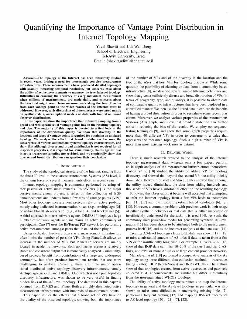
Accounting for these possibly mis-identified VPs, we filter out allthe measurements for which tr(ai, vpj) < T , i.e., agent ai measuredfrom VP vpj less than T traceroutes. Applying this filter with T =200, reduces the number of agents that have more than 5 differentVPs to less than 0.55% of the agents and leaves no agent that havemore than 10 different VPs. Filtering with T = 500 yields less than0.4% of the agents with more than 5 VPs. Since there is a trade-offbetween the accuracy of VP identification and loss of data due toover-filtering, we select T = 200 and estimate the extent of mis-identification errors.
The VP identification error of an agent is estimated as the per-centage of measurements it performed from VPs suspected as mis-identified out of the overall number of its measurements. More for-mally, consider tr(ai, vpj) to be the number of traceroutes performedby agent ai from VP vpj ∈ V , and the indicator xj which marks apossibly mis-identified VP:
∀j ∈ {1..|V |}, xj ={
1 tr (ai, vpj) < T0 otherwise
The VP identification error is thus given by:
err (aj) = 100 ·∑j xj · tr(ai, vpj)∑j tr(ai, vpj)
Using T = 200, Fig. 1 plots the cumulative distribution of theerror estimation (right) and the mis-identification error as a functionof the total number of measurements per agent. Most agents (73%)have no mis-identification error and only 7 agents (less than 1%)have 100% error estimation. Out of these, only 2 have more than5,000 measurements, making these an indication of error since theirmeasurements span across multiple (mis-identified) ASes, for eachat most 200 measurements are performed. The overall error, i.e., thepercentage of all measurements that are suspected as mis-identifiedout of the total measurements performed by all agents, is 0.23%(marked by the red line in the right plot), indicating that only a fewagents (less than 4%) contribute most of the mis-identification, as canalso be seen by the few marks above the zero line in the left plot.In the remainder of the paper, we use only measurements for whichtr(ai, vpj) ≤ T, T = 200, and refer to it as the filtered data.
102
103
104
105
106
0
10
20
30
40
50
60
70
80
90
100
Number of measurements
Err
or
estim
atio
n (
pe
rce
nt)
10−4
10−2
100
102
75
80
85
90
95
100
Error estimation (percent)
Pe
rce
nte
of
ag
en
ts
Fig. 1: Estimation of error in the identification of VPs
100
102
104
100
101
102
103
Vantage point degree
Ave
rag
e n
um
be
r o
f a
ge
nts
Filtered
Unfiltered
100
102
10410
0
102
104
106
108
Vantage point degree
Ave
rag
e n
um
be
r o
f m
ea
su
rem
en
ts
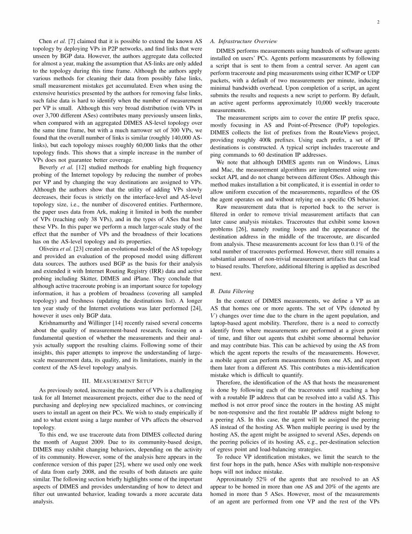
Fig. 2: Average number of agents and measurements per VP degree.Filtered data includes only agents from VPs where tr(ai, vpj) ≥ 200
For each vpi we extract the number of measuring agents,agents(vpi) and the number of total traceroute measurements per-formed from it, tr(vpi). Using the degree ki of its hosting AS in theundirected AS graph, i.e., number of links to neighboring ASes, wecalculate the average number of traceroute measurements per degree:
tr(k) =
∑i∈{ki=k}
tr(vpi)
|{i|ki = k}|and average number of agents per AS degree:
agents(k) =
∑i∈{ki=k}
agents(vpi)
|{i|ki = k}|
We repeat this calculation for the filtered set, and find trf (k) andagentsf (k).
Fig. 2 (left) shows that VPs with higher degree tend to havemore agents. Using degrees extracted from RouteViews producedthe same results, indicating that this is not a sampling bias causedby measurement artifacts [27], i.e., the high degree is not the resultof having more agents but rather an indication that large ASes tendto “host” more agents. Additionally, Fig. 2 (right) shows no directrelationship between the number of measurements and the VP degree,showing that there is a good distribution of measuring agents acrossthe different ASes.
C. Measurement Time-frame
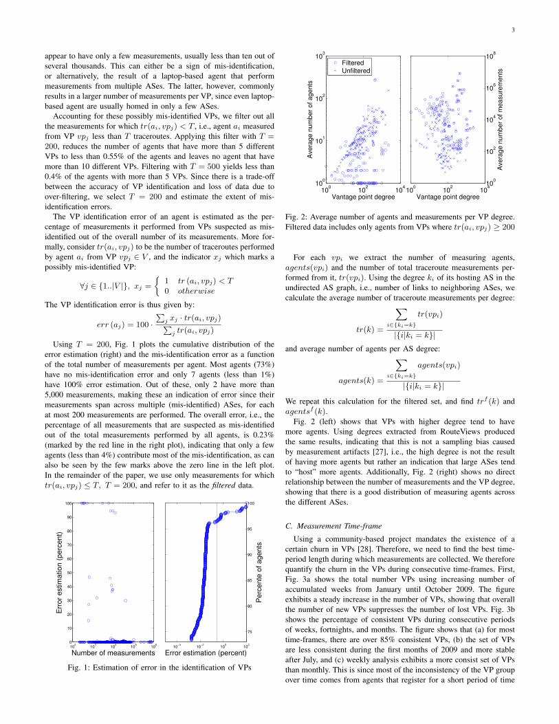
Using a community-based project mandates the existence of acertain churn in VPs [28]. Therefore, we need to find the best time-period length during which measurements are collected. We thereforequantify the churn in the VPs during consecutive time-frames. First,Fig. 3a shows the total number VPs using increasing number ofaccumulated weeks from January until October 2009. The figureexhibits a steady increase in the number of VPs, showing that overallthe number of new VPs suppresses the number of lost VPs. Fig. 3bshows the percentage of consistent VPs during consecutive periodsof weeks, fortnights, and months. The figure shows that (a) for mosttime-frames, there are over 85% consistent VPs, (b) the set of VPsare less consistent during the first months of 2009 and more stableafter July, and (c) weekly analysis exhibits a more consist set of VPsthan monthly. This is since most of the inconsistency of the VP groupover time comes from agents that register for a short period of time
4
(or laptops taken on trips to uncommon locations) and not due toagents that stop working for a week or two, which is also seen fromthe constant increase in Fig. 3a. Thus, looking at longer time perioddoes the opposite of smoothening the data.
10 15 20 25 30 35 40Last accumulated week index
100
150
200
250
300
350
Tota
l num
ber o
f VPs
(a) Accumulated
10 15 20 25 30 35 40Week index
75
80
85
90
95
100
Perc
ent o
f con
sist
ent V
Ps
WeeklyBi-WeeklyMonthly
(b) Consistency
Fig. 3: VP churn during 2009 showing that (a) accumulating weeksresults in a steady increase of the the VP count, and (b) VPs exhibitless churn on shorter time frames
These observations lead us to use data collected for a completemonth during August 2009, where the churn is low. This helps obtaina set of relatively consistent VPs, allowing easier analysis of the largedataset. Moreover, using a complete month, increases the probabilitythat there is a good coverage of the underlying topology, meaningthat most ASes and AS-links are observed by more than one agent.
IV. VANTAGE POINTS DISTRIBUTION ANALYSIS
This section provides an in depth analysis of the various aspectsrelated to the distribution of VPs and its effect on the resultingtopology features.
A. Diminishing Returns
We now have the data needed to revisit the diminishing returnsclaim by examining how the observed topology changes as data frommore VPs is added. Evaluating the effect of adding VPs is done byfirst building the local AS topology as observed from each of theVPs, i.e., the AS topology measured by agents when they are hostedin each VP.
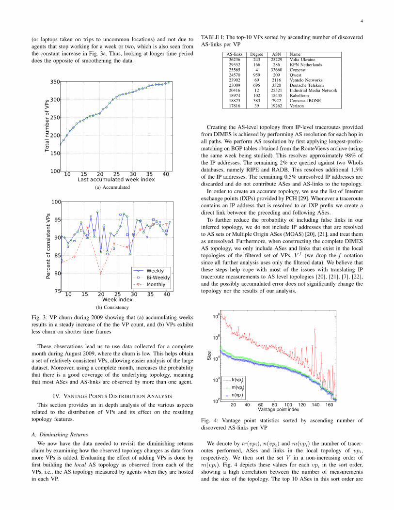
TABLE I: The top-10 VPs sorted by ascending number of discoveredAS-links per VP
Creating the AS-level topology from IP-level traceroutes providedfrom DIMES is achieved by performing AS resolution for each hop inall paths. We perform AS resolution by first applying longest-prefix-matching on BGP tables obtained from the RouteViews archive (usingthe same week being studied). This resolves approximately 98% ofthe IP addresses. The remaining 2% are queried against two WhoIsdatabases, namely RIPE and RADB. This resolves additional 1.5%of the IP addresses. The remaining 0.5% unresolved IP addresses arediscarded and do not contribute ASes and AS-links to the topology.
In order to create an accurate topology, we use the list of Internetexchange points (IXPs) provided by PCH [29]. Whenever a traceroutecontains an IP address that is resolved to an IXP prefix we create adirect link between the preceding and following ASes.
To further reduce the probability of including false links in ourinferred topology, we do not include IP addresses that are resolvedto AS sets or Multiple Origin ASes (MOAS) [20], [21], and treat themas unresolved. Furthermore, when constructing the complete DIMESAS topology, we only include ASes and links that exist in the localtopologies of the filtered set of VPs, V f (we drop the f notationsince all further analysis uses only the filtered data). We believe thatthese steps help cope with most of the issues with translating IPtraceroute measurements to AS level topologies [20], [21], [7], [22],and the possibly accumulated error does not significantly change thetopology nor the results of our analysis.
20 40 60 80 100 120 140 16010
2
103
104
105
106
Vantage point index
Siz
e
tr(vpi)
m(vpi)
n(vpi)
Fig. 4: Vantage point statistics sorted by ascending number ofdiscovered AS-links per VP
We denote by tr(vpi), n(vpi) and m(vpi) the number of tracer-outes performed, ASes and links in the local topology of vpi,respectively. We then sort the set V in a non-increasing order ofm(vpi). Fig. 4 depicts these values for each vpi in the sort order,showing a high correlation between the number of measurementsand the size of the topology. The top 10 ASes in this sort order are
5
provided in Table I. This correlation, however, breaks at the tail ofthe ordered list.
We use this sort order in the following sections in order to quantifythe effect of VP aggregation on various topology parameters. Wepoint out that VPs that discover the largest local topologies aremostly located in Europe and the United States. Out of the top tenVPs, 7 are in the Europe and 3 are in USA (Qwest, Comcast andVerizon). Only the 13th VP is the first in a different geographicalregion (Israel) and the 30th is in Australia. This means that “remote”regions that are outside the areas used by other instrumented activemeasurement projects (e.g., Ark), and are likely to introduce newcontributions to the AS topology, are considered only later in thissorted VP list. Table I shows that ASes with large degrees as wellas ASes with medium and small degrees are represented in the top10 largest topologies, indicating that our order is not slanted towardshigh degree ASes.
0 20 40 60 80 100 120 140 160Vantage points
0
1
2
3
4
5
6
7
8
Topo
logy
siz
e
�104
AS linksASes
(a) Topology
0 20 40 60 80 100 120 140 160Vantage points
100
101
102
103
104
�
topo
logy
siz
e
AS linksASes
(b) ∆ Topology
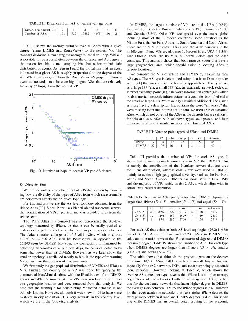
Fig. 5: Number of ASes and AS-links in the aggregated topology
B. Aggregation of Local Topologies
Once we have the sorted set V we build a set of aggregated AStopologies, Agg. An aggregated topology aggi includes the ASesand links from the set of local topologies, aggi = ∪ij=1vpj . Fig. 5adepicts the size of the aggregated topology as a function of thenumber of VPs and Fig. 5b depicts the contribution of each VP to theaggregate growth. The number of ASes almost reaches its final valueafter aggregating only a few VPs. We note that the full set of ASes
0 20 40 60 80 100 120 140 160Vantage points
0
500
1000
1500
2000
2500
3000
3500
4000
Deg
ree
Max degreeMax difference
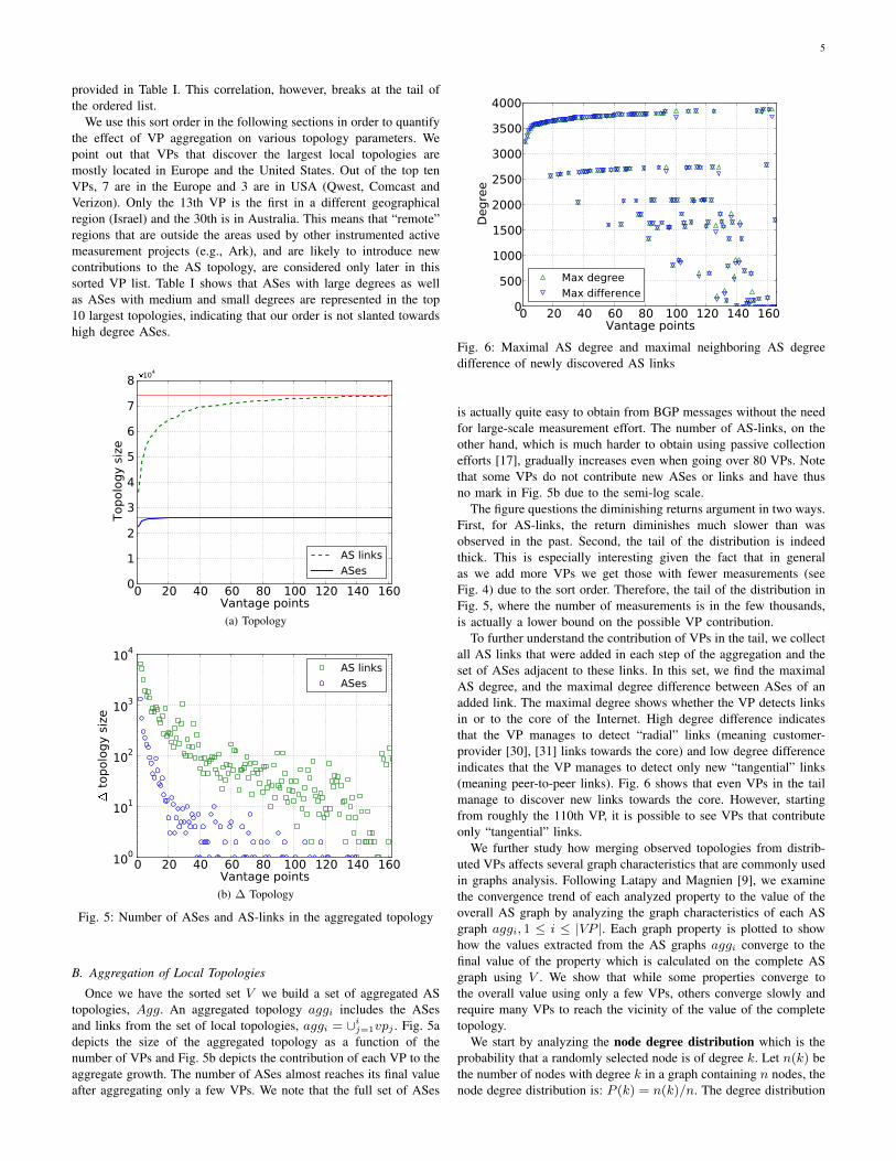
Fig. 6: Maximal AS degree and maximal neighboring AS degreedifference of newly discovered AS links
is actually quite easy to obtain from BGP messages without the needfor large-scale measurement effort. The number of AS-links, on theother hand, which is much harder to obtain using passive collectionefforts [17], gradually increases even when going over 80 VPs. Notethat some VPs do not contribute new ASes or links and have thusno mark in Fig. 5b due to the semi-log scale.
The figure questions the diminishing returns argument in two ways.First, for AS-links, the return diminishes much slower than wasobserved in the past. Second, the tail of the distribution is indeedthick. This is especially interesting given the fact that in generalas we add more VPs we get those with fewer measurements (seeFig. 4) due to the sort order. Therefore, the tail of the distribution inFig. 5, where the number of measurements is in the few thousands,is actually a lower bound on the possible VP contribution.
To further understand the contribution of VPs in the tail, we collectall AS links that were added in each step of the aggregation and theset of ASes adjacent to these links. In this set, we find the maximalAS degree, and the maximal degree difference between ASes of anadded link. The maximal degree shows whether the VP detects linksin or to the core of the Internet. High degree difference indicatesthat the VP manages to detect “radial” links (meaning customer-provider [30], [31] links towards the core) and low degree differenceindicates that the VP manages to detect only new “tangential” links(meaning peer-to-peer links). Fig. 6 shows that even VPs in the tailmanage to discover new links towards the core. However, startingfrom roughly the 110th VP, it is possible to see VPs that contributeonly “tangential” links.
We further study how merging observed topologies from distrib-uted VPs affects several graph characteristics that are commonly usedin graphs analysis. Following Latapy and Magnien [9], we examinethe convergence trend of each analyzed property to the value of theoverall AS graph by analyzing the graph characteristics of each ASgraph aggi, 1 ≤ i ≤ |VP |. Each graph property is plotted to showhow the values extracted from the AS graphs aggi converge to thefinal value of the property which is calculated on the complete ASgraph using V . We show that while some properties converge tothe overall value using only a few VPs, others converge slowly andrequire many VPs to reach the vicinity of the value of the completetopology.
We start by analyzing the node degree distribution which is theprobability that a randomly selected node is of degree k. Let n(k) bethe number of nodes with degree k in a graph containing n nodes, thenode degree distribution is: P (k) = n(k)/n. The degree distribution
6
0 20 40 60 80 100 120 140 160Vantage points
3.0
3.5
4.0
4.5
5.0
5.5
6.0Av
erag
e de
gree
(a) Average AS Degree
0 20 40 60 80 100 120 140 160Vantage points
2.10
2.15
2.20
2.25
2.30
2.35
2.40
2.45
PDF
expo
nent
�
(b) PDF Exponent
0 20 40 60 80 100 120 140 160Vantage points
1000
2000
3000
4000
5000
6000
7000
8000
Deg
ree
kPLmax
kmax
(c) Maximal Degree
0 20 40 60 80 100 120 140 160Vantage points
10
20
30
40
50
60
70
Core
inde
x / N
umbe
r of A
Ses Core size
kmax
(d) k-core
0 20 40 60 80 100 120 140 160Vantage points
0.08
0.10
0.12
0.14
0.16
0.18
0.20
0.22
Max
bet
wee
nnes
s ce
ntra
lity
(e) Betweenness Centrality
0 20 40 60 80 100 120 140 160Vantage points
0.75
0.76
0.77
0.78
0.79
0.80
0.81
Aver
age
clus
terin
g co
effic
ient
(f) Clustering Coefficient
Fig. 7: Topology characteristics analysis of aggregated AS graphs. The horizontal line marks the value calculated on the complete AS graph
has became one of the most frequently analyzed Internet topologycharacteristics [19] since the work of Faloutsos et al. [15] that showedthat the degree distribution of Internet topologies follows a power-law, meaning P (k) ∼ k−γ , where γ is a positive exponent. We usethe closely related Zipf [32] distribution, n(k) ∼ k−α, and calculateγ = 1/α+ 1.
Fig. 7a and Fig. 7b show that the average degree and PDF exponentmonotonically converge, reaching the vicinity (within 10%) of theoverall value after roughly 40 VPs, and 120 VPs to reach within 1%of the overall value. Interestingly, the exponent value we get usingall VPs (γ = 2.14) is quite similar to the one reported by Faloutsoset al. [15] who used a single VP ten years ago (γ ' 2.20).
Fig. 7c shows that the maximum degree converges even faster, in-dicating that the first few VPs accurately map the highest degree AS,namely Level3 (AS-3356). We also plot a theoretical maximum nodedegree in a power-law degree distribution, kPLmax = n1/(γ−1) [33].The theoretical maximum degree starts by converging nicely to thetrue maximal degree. If we had only about 10 VPs we would believethat the formula works well for the Internet AS graph. However,as we keep adding more VPs, kPLmax climb very fast and eventuallyreaches a value, which is almost double the true maximal degree.A similar deviation from the strict power-law model, observed in[34], was attributed to the mixture of customer-provider links andpeering links, having the first follow the model whereas the latter donot. Indeed, as is seen in Fig. 6, the first VPs detect mostly radialcustomer-provider links whereas VPs farther in the list detect morepeer-to-peer links, causing the observed deviation from the power-lawmodel. Overall, these findings further strengthen the recent claimsagainst the accuracy of the power-law model for Internet topology[14], [16].
k-Pruning [35] is a method for decomposing graphs into shells,having each node being mapped to a shell based on its connectivity.Nodes in the first shell are those who have only one link leading tothe ‘center’ of the graph. Nodes in the kth shell have k-connectivity
towards the center. The nucleus (or core) is the shell with the highestindex, kmax. Fig. 7d plots the value of kmax and the number ofASes in the core, when applying k-shell analysis on the aggregatedAS graphs.
The nucleus index, shown in Fig. 7d, converges to 10% of itsoverall value (kmax = 31) after over 60 VPs. Additionally, thenumber of ASes in the nucleus is dynamic as we add more VPs.The drops we see in the number of ASes in the core is due tothe separation of the core into two shells at the points where kmaxincreases, as more links are added. These changes occur even whenthe number of VPs is well over 100.
20 40 60 80 100 120 140 160Vantage points
1743257332064535511127379224766463771321200
154121257812
32924436
2597347884657
4109594984775
ASN
in c
ore
0
10
20
30
40
50
60
70
Num
ber o
f ASe
s in
cor
e
Fig. 8: AS membership in the nucleus of the aggregated AS graphs
In order to further understand the dynamics of the core, we lookedat the ASes that are in the core and their connectivity. Fig. 8 depictsthe core ASes in each aggregated topology. Each horizontal linerepresent the membership of a specific AS (not all AS numbers are
7
shown for brevity of the plot) in the aggregations by a dot wherethe AS was a core member of aggi. The right y-axis shows theoverall number of ASes (number of dots in each aggi) in the core,which is illustrated by the line. The figure shows that the true core iscomprised of about 43 ASes that are present in all the aggregationsafter roughly 90 VPs, and additional 20 or so join and leave thecore almost simultaneously. The simultaneous departure is the resultof detecting more links in the core, which in turn increases theconnectivity between the real core ASes and causes them to separateinto a new higher shell. This can also be seen in Fig. 7d, by observingthat each drop in the number of ASes in the core after the 60thaggregation, is perfectly aligned with the increase in the core index(kmax). We also observed that the average degree of the ASes inthe true core graph (i.e., not their overall degree, but their degreeafter the pruning process) is roughly 40, indicating that the core isdense, with almost a full mesh structure. However, when the corebecomes larger with more than 60 ASes, the average degree doeschange, making the core sparse. Another important observation isthat in the first 16 aggregations, there are about 20 VPsthat are notseen afterwards, indicating that they are mistakingly included in thecore due to insufficient aggregation.
Given that the core extracted using k-pruning captures a globalview of the Internet top-level providers [35], it holds both tier-1 andtier-2 ASes, hence even if finding most tier-1 links can be done onlyBGP data [18], it takes a much more comprehensive probing to findthe complete Internet core. This indicates that finding links in theInternet core, which captures a broader concept than tier-1 ASes, isnot as easy as is believed.
Betweenness centrality (bc) is commonly used for measuring thecentrality of a node or a link. Node betweenness measures the numberof shortest paths passing through a node as an estimate to the potentialtraffic load on this node assuming uniformly distributed traffic whichfollows shortest paths [19]. We calculate the maximal betweennessover all ASes in each Aggj as a measure for possible congestednodes in the graph. In order to compare topologies with differentsizes, we normalize the average betweenness by the maximal possiblebetweenness value, nj(nj − 1). Fig. 7e shows that bc convergeswithin 10% of the overall value after roughly 20 VPs. Since bc is ameasure of load, adding links almost always decreases the averageload on ASes (except pathologies like the Braess paradox), thus themonotonic descent. Since high-degree ASes are more “central” thanlow-degree ASes, we expect that tier-1 ASes will have the maximalbetweenness values. Indeed, Level3 (AS3356), a tier-1 AS, is the ASwith the maximal bc for all resulting graphs.
Clustering Coefficient (cc) of a graph measures the local cliquish-ness of a node neighborhood [36]. Simply put, clustering coefficientestimates how close a given node and its immediate neighbors arefrom being a clique. A graph average clustering coefficient is usedto estimate how close a graph is to a small-world network, suchthat graphs with higher average clustering coefficient can be bettermodeled by a small-world network. Fig. 7f shows that the cc issurprisingly estimated to within 2% of the final value after only 3VPs and stays within this narrow distance from the final value whilejugging up and down. The value reported here, which is roughly 0.76,is quite different from what was reported for topologies collected inthe Skitter project (0.46) and WHOIS repositories (0.49) [19].
In the conference version of this paper [25] we presented most ofthe analysis of this subsection but for a single week in early 2008.While the topologies (both per VP and the aggregates) are now largerby almost 60%, the convergence properties are similar.
C. Sampling Bias
Several studies [27], [37], [38] analyze the bias that the commonlyused traceroute sampling method potentially introduces into theinferred topology. In [27] the router-level topology inferred usingtraceroute sampling was shown to be biased by the distance betweenthe measuring VP and the probed interface. This claim was partiallyconfronted by showing [37] that that various traceroute explorationstrategies can produce topologies with minimal bias.
We expect that achieving a broad distribution of VPs, alongsidewith the relatively low diameter of the AS-level topology, shouldresult in a good sampling process of the underlying topology so thatit will exhibit less bias that result from the distance between VPs andobserved ASes.
Measuring the distance between VPs to ASes is done by searchingfor the shortest valley-free path between each VP and the ASes itobserves. A valley-free path follows a strict hierarchical structure– an uphill segment of zero or more customer-provider or siblinglinks, followed by zero or one peer-to-peer link, followed by adownhill segment of zero or more provider-customer or sibling links.For this end, we customized the shortest-path Dijkstra algorithmto obey the valley-free routing rules. Calculating a valley-free pathrequires the inference of the type-of-relationship between adjacentASes (customer-provider, peers or siblings) in the AS graph. The rela-tionships are inferred using the near-deterministic type-of-relationshipalgorithm [31].
First, for each AS we find all the VPs that include it in theirobserved topology (referred to as “observing VPs”), and calculate thenumber of hops from the AS to each of them. Fig. 9 shows the averagenumber of observing VPs calculated over all ASes with a givendegree obtained from DIMES and RouteViews AS-level topologies.As expected, the figure shows that low-degree ASes are observedfrom much fewer VPs than high-degree ASes. This is attributed to thefact that small degree ASes are harder to detect and probe. However,there are a few ASes that have high degree (mostly in RouteViews)and are observed by only few VPs, but these are quite rare.
100
101
102
103
104
0
20
40
60
80
100
120
140
AS degree
Avera
ge n
um
ber
of observ
ing V
Ps
DIMES degree
RV degree
Fig. 9: Number of observing VPs per AS degree
Table II shows the distribution of the number of ASes per distanceto the nearest observing VP. The table shows that most ASes are 1 to3 hops away from the nearest VP, 191 ASes serve as VPs (thus arezero hops away), and a small fraction of ASes (just over a hundred)have VPs that are 4 or 5 hops away. The average distance is 1.9 hopswith a standard deviation of 0.62, and the median is 2 hops, showingthat the set of VPs are well spread.
8
TABLE II: Distances from AS to nearest vantage point
Distance to nearest VP 0 1 2 3 4 5Number of ASes 191 4727 17482 4695 106 2
Fig. 10 shows the average distance over all ASes with a givendegree (using DIMES and RouteViews) to the nearest VP. Thestandard deviation surrounding the average is less than 1 hop. While itis possible to see a correlation between the distance and AS degrees,the reason for this is not sampling bias but rather probabilisticdistribution of agents. As seen in Fig. 2 the probability that an agentis located in a given AS is roughly proportional to the degree of theAS. When using degrees from the RouteViews AS graph, the bias iseven less noticed, since there are high-degree ASes that are relativelyfar away (2 hops) from the nearest VP.
100
101
102
103
104
0
0.5
1
1.5
2
2.5
AS degree
Ave
rag
e h
op
s t
o n
ea
rest
VP
DIMES degree
RV degree
Fig. 10: Number of hops to nearest VP per AS degree
D. Diversity Bias
We further wish to study the effect of VPs distribution by examin-ing how the diversity of the types of ASes from which measurementsare performed affects the observed topology.
For this analysis we use the AS-level topology obtained from theiPlane Atlas [39]. Since iPlane uses PlanetLab and traceroute servers,the identification of VPs is precise, and was provided to us from theiPlane team.
The iPlane Atlas is a compact way of representing the AS-leveltopology measured by iPlane, so that it can be easily pushed toend-users for path prediction applications in peer-to-peer networks.The Atlas contains a large set of 31,611 ASes, which is almostall of the 32,326 ASes seen by RouteViews, as opposed to the27,203 seen by DIMES. However, the connectivity is measured bycollecting traceroutes of only a few days, hence is expected to besomewhat lower than in DIMES. However, as we later show, thesmaller topology is attributed mostly to bias in the type of measuringVP rather than the duration of measurements.
We first study the geographical distribution of DIMES and iPlane’sVPs. Finding the country of a VP was done by querying thecommercial MaxMind database with the IP addresses of the DIMESagents and iPlane’s sources. A few VPs were resolved to more thanone geographic location and were removed from this analysis. Wenote that the technique for constructing MaxMind database is notpublicly known. However, although it was shown [40] to have somemistakes in city resolution, it is very accurate in the country level,which we use in the following analysis.
In DIMES, the largest number of VPs are in the USA (40.8%),followed by UK (8%), Russian Federation (7.3%), Germany (6.5%)and Canada (5.8%). Other VPs are spread over the entire globe,including most of the European countries, some countries in theMiddle East, the Far East, Australia, South America and South Africa.There are no VPs in Central Africa and the Arab countries in themiddle east. iPlane VPs are also mostly located in the USA (43.3%).Like DIMES, there are no VPs in Central Africa and the Arabcountries. This analysis shows that both projects cover a relativelylarge geographical area, which should assist in locating ASes inremote locations.
We compare the VPs of iPlane and DIMES by examining theirAS types. The AS type is determined using data from Dimitropouloset al. [41] that uses a machine learning approach to classify an ASas a large ISP (t1), a small ISP (t2), an academic network (edu), anInternet exchange point (ix), a network information center (nic) whichholds important network infrastructure, or a customer (comp) of eitherthe small or large ISPs. We manually classified additional ASes, suchas those having a description that contains the word “university” thatwere missing from the inferred set. In total we used 18,639 classifiedASes, which do not cover all the ASes in the datasets but are sufficientfor this analysis. ASes with unknown types are ignored, and bothinfrastructures have a similar number of unclassified ASes.
TABLE III: Vantage point types of iPlane and DIMES
t1 t2 edu comp ix nic unknowniPlane 17 104 117 22 3 5 46DIMES 29 106 10 11 2 1 47
Table III provides the number of VPs for each AS type. Itshows that iPlane uses much more academic VPs than DIMES. Thisis mainly the contribution of the PlantLab servers that are usedfor iPlane distribution, whereas only a few were used in DIMES,mainly to achieve high geographical diversity, such as the Far East,Africa and South America. DIMES has more VPs in tier-1 ISPsand the majority of VPs reside in tier-2 ASes, which align with itscommunity-based distribution.
TABLE IV: Number of ASes per type for which DIMES degrees arelarger than iPlane (D > P ), smaller (D < P ) and equal (D = P )
t1 t2 edu comp ix nic unknownD > P 26 2392 309 2436 20 70 4239D < P 17 1198 153 1679 4 49 2410D = P 1 974 283 3760 4 54 5349
For each AS that exists in both AS-level topologies (26,261 ASesout of 31,611 ASes in iPlane and 27,203 ASes in DIMES), wecalculated the ratio between the iPlane measured degree and DIMESmeasured degree. Table IV shows the number of ASes for each typewhen DIMES degrees are larger than iPlane’s (D > P ), smaller(D < P ) and equal (D = P ).
The table shows that although the projects agree on the degreesof almost 10,500 ASes, DIMES exhibits overall higher degrees,especially for tier-2 networks, IXPs, and most surprisingly academic(edu) networks. However, looking at Table V, which shows theaverage AS degree per type, reveals that iPlane has a higher averagedegree for academic networks. Further examining these ASes, we findthat for the academic networks that haver higher degree in DIMES,the average ratio between DIMES and iPlane degrees is 2.4. However,for the fewer academic networks that have higher iPlane degree, theaverage ratio between iPlane and DIMES degrees is 4.2. This showsthat while DIMES has an overall better probing of the academic
9
networks, as it has for the majority of the observed ASes, iPlane hasa significantly better view of some of these networks.
100
101
102
103
104
100
101
102
103
104
DIMES Degrees
iPla
ne D
egre
es
t1
t2
edu
Fig. 11: Comparison of iPlane and DIMES degrees for tier-1, tier-2and academic networks (edu)
These observations are further depicted in Fig. 11, which shows ascatter plot of iPlane degree vs. DIMES degree for tier-1, tier-2 andacademic ASes. The figure shows that for the vast majority of tier-1and tier-2 ASes both topologies degrees are similar, while for someacademic networks iPlane measures significantly higher degrees thanDIMES.
The two infrastructures agree on the degree of only a single tier-1 AS (AS372 Korea Telecom, degree 372). However, the averagedegree of tier-1 ASes is very high (more than 600 for both projects),hence the chances to agree are low. Moreover, although the averageratio of degrees (DIMES/iPlane) for tier-1 ASes is 2.04, the standarddeviation is 6.7, showing that the degrees are relatively similar butthe variance is high.
TABLE V: Average AS degrees using RouteViews, DIMES andiPlane per AS type
t1 t2 edu comp ix nic unknownRouteViews 606.2 9.9 3.0 2.3 6.4 4.7 5.1DIMES 864.5 15.0 4.3 3.0 75.2 5.5 9.0iPlane 656.0 15.1 5.6 2.7 18.2 8.1 6.3
Table V compares average AS degrees per AS type of the DIMES,iPlane, and RouteViews AS graphs. RouteViews passively collectsBGP messages and is considered a reliable source for the AStopology, although it can miss links between ASes that do notparticipate in BGP, which is more common in tier-2 ASes [17].Table V provides the average AS degree per type using data collectedduring August 2009 and the iPlane Atlas. It shows that for allAS types RouteViews has the lowest average degrees. As statedbefore, iPlane observes higher average degree in academic networksnetworks, whereas DIMES has higher degrees in tier-1 and IXPs.These differences are attributed to bias that each project holds towardsits VP types. The observation that DIMES has much higher degree forIXPs is mostly attributed to incorrect inference of their connectivity,whereas the iPlane Atlas employs more accurate connectivity analysis[39] for IXPs. Interestingly, the average degree of tier-2 ASes isalmost identical in DIMES and iPlane, while both are 50% morethan RouteViews. This can possibly be attributed to the difference inthe probing method (active vs. passive) and placement of VPs.
TABLE VI: Average VP degree per type, calculated over origin ASesof iPlane, DIMES and both
VPs Avg. Degree t1 t2 edu comp ix niciPlane iPlane 1004 51.1 19 6 20 3.6
Finally, we evaluate how the presence of a VP within an AS affectsits observed connectivity to other ASes. Table VI provides the averageVP degree per type, calculated over VPs of iPlane, DIMES and both.Strengthening the above observations, DIMES has higher averagedegrees for almost all VPs except academic networks, which arethe primary distribution method of iPlane. Interestingly, DIMES hashigher degrees in tier-1 ASes that are not part of its VP set. Weattribute this mostly to the relatively easy probing of tier-1 ASes,as many traceroutes pass through them [35], therefore enabling easyprobing even from the “outside”.
E. Discussion
The above analysis illustrates several important results. First, itshows that although increasing the number of VPs can help reducingsampling bias, it still does not guarantee unbiased results. Althoughboth iPlane and DIMES have a very broad distribution, the types ofASes in which their VPs are located generate a topology that is biasedtowards these types. Most obvious are the academic networks whichare probed significantly better in iPlane than in DIMES. Overcomingthis bias cannot be achieved by simply increasing the number of VPsbut rather a broad diversity in types is required.
Second, the analysis strengthens the assumption that measuringfrom within a network is important for discovering more of its links,mainly for low-tier ASes, as these are harder to probe than tier-1ASes. However, it also exposes that using a large spread of VPs, thatperform many measurements for a sufficient period, can still resultin extensive coverage of networks, even from the “outside” of thenetwork.
Finally, we found that in tier-2 ASes both iPlane and DIMEShave significantly higher degrees than RouteViews. We attributethis to several key features of Internet measurement efforts. First,DIMES and iPlane have significantly more VPs than RouteViews,especially in these lower level ASes, enabling better probing. Second,RouteViews mostly measures from the core of the Internet whileiPlane and even to a greater extent DIMES, measure from the farreaches of the Internet. Due to the valley-free routing policy, certaintypes of peer-to-peer links are only visible from the customers of thepeering ASes [11], [34]. Thus, the location of VPs in these ASes isrequired in order to gain a good coverage and have a more completeview of the Internet topology. Finally, RouteViews uses passivecollection of BGP messages, hence it is only capable of capturinglinks that are published in BGP. In recent years, there is an increasingusage of private peering between ASes [42], [43], making these linksvisible only to active probing. Although active measurements aremore challenging to analyze, the benefits of improved probing ofnetworks is significant.
V. CONCLUSION
This paper presents an analysis of the significance of the distri-bution of vantage points (VPs) in an active Internet measurementinfrastructure. We showed that diverse and broad distribution can
10
help overcome sampling bias and uncover hidden parts of the Inter-net topology. However, even broadly distributed infrastructures stillexhibit some bias towards the type of ASes from which measurementsare performed, further stressing the need for a diversity of VP typesand geographic locations. To this end, community based infrastruc-tures are well suited since their growth potential is theoreticallyunlimited. Looking at various commonly analyzed graph properties,we showed that some require more than 40 VPs to converge, butsurprisingly several others converge with only a few VPs.
REFERENCES
[1] University of Oregon Advanced Network Technology Center, “RouteViews Project, http://www.routeviews.org/.”
[2] CAIDA Macroscopic Topology Project Team, “Caidaarchipelago, next generation active measurement infrastructure(http://imdc.datcat.org/collection/).”
[3] B. Chun, D. Culler, T. Roscoe, A. Bavier, L. Peterson, M. Wawrzoniak,and M. Bowman, “PlanetLab: An overlay testbed for broad-coverageservices,” ACM SIGCOMM Computer Communications Review, vol. 33,no. 3, Jul. 2003.
[4] H. V. Madhyastha, T. Isdal, M. Piatek, C. Dixon, T. E. Anderson,A. Krishnamurthy, and A. Venkataramani, “iPlane: An information planefor distributed services,” in OSDI, 2006, pp. 367–380.
[5] N. T. Spring, R. Mahajan, and D. Wetherall, “Measuring ISP topologieswith Rocketfuel,” in SIGCOMM, 2002, pp. 133–145.
[6] Y. Shavitt and E. Shir, “DIMES: Let the Internet measure itself,” ACMSIGCOMM Computer Communications Review, vol. 35, no. 5, 2005.
[7] K. Chen, D. R. Choffnes, R. Potharaju, Y. Chen, F. E. Bustamante,D. Pei, and Y. Zhao, “Where the sidewalk ends: Extending the internetAS graph using traceroutes from P2P users,” in ACM CoNEXT, Dec.2009.
[8] kc claffy, M. Crovella, T. Friedman, C. Shannon, and N. Spring,“Community-oriented network measurement infrastructure (conmi)workshop report,” SIGCOMM Computer Communication Review,vol. 36, no. 2, pp. 41–48, 2006.
[9] M. Latapy and C. Magnien, “Complex network measurements: Estimat-ing the relevance of observed properties,” in IEEE Infocom, 2008.
[10] P. Barford, A. Bestavros, J. Byers, and M. Crovella, “On the marginalutility of network topology measurements,” in IMW’01: the 1st ACMSIGCOMM Workshop on Internet Measurement, 2001, pp. 5–17.
[11] R. Cohen and D. Raz, “The Internet dark matter - on the missing links inthe AS connectivity map,” in IEEE INFOCOM, Barcelona, Spain, Apr.2006.
[12] R. Beverly, A. Berger, and G. G. Xie, “Primitives for active Internettopology mapping: Towards high-frequency characterization,” in IMC,2010.
[13] D. Achlioptas, A. Clauset, D. Kempe, and C. Moore, “On the biasof traceroute sampling: or, power-law degree distributions in regulargraphs,” in STOC. Baltimore, MD, USA: ACM, 2005, pp. 694–703.
[14] B. Krishnamurthy and W. Willinger, “What are our standards forvalidation of measurement-based networking research?” SIGMETRICSPerform. Eval. Rev., vol. 36, pp. 64–69, Aug. 2008.
[15] M. Faloutsos, P. Faloutsos, and C. Faloutsos, “On power-law relation-ships of the Internet topology,” ACM SIGCOMM Computer Communi-cations Review, vol. 29, no. 4, pp. 251–262, 1999.
[16] Q. Chen, H. Chang, R. Govindan, S. Jamin, S. J. Shenker, and W. Will-inger, “The origin of power laws in Internet topologies revisited,” inINFOCOM, 2002, pp. 608–617 vol.2.
[17] R. V. Oliveira, D. Pei, W. Willinger, B. Zhang, and L. Zhang, “Insearch of the elusive ground truth: the Internet’s AS-level connectivitystructure,” in SIGMETRICS. ACM, 2008, pp. 217–228.
[18] R. Oliveira, D. Pei, W. Willinger, B. Zhang, and L. Zhang,“The (in)completeness of the observed Internet AS-level structure,”IEEE/ACM Transactions on Networking, vol. 18, pp. 109–122, February2010.
[19] P. Mahadevan, D. Krioukov, M. Fomenkov, B. Huffaker, X. Dimitropou-los, kc claffy, and A. Vahdat, “The Internet AS-level topology: Threedata sources and one definitive metric,” ACM SIGCOMM ComputerCommunications Review, vol. 36, p. 17, 2006.
[20] Z. Mao, J. Rexford, J. Wang, and R. H. Katz, “Towards an accurateAS-level traceroute tool,” in SIGCOMM, 2003.
[21] Z. Mao, D. Johnson, J. Rexford, J. Wang, and R. H. Katz, “Scalableand accurate identification of AS-level forwarding paths,” in INFOCOM,2004.
[22] “TraceNET: an Internet topology data collector,” in IMC. ACM, 2010.[23] R. V. Oliveira, B. Zhang, and L. Zhang, “Observing the evolution of
Internet AS topology,” ACM SIGCOMM Computer CommunicationsReview, vol. 37, no. 4, pp. 313–324, 2007.
[24] A. Dhamdhere and C. Dovrolis, “Ten years in the evolution of theInternet ecosystem,” in IMC. ACM, 2008, pp. 183–196.
[25] Y. Shavitt and U. Weinsberg, “Quantifying the importance of vantagepoints distribution in internet topology measurements,” in Infocom, Riode Janeiro, Brazil, Apr. 2009.
[26] B. Augustin, X. Cuvellier, B. Orgogozo, F. Viger, T. Friedman, M. Lat-apy, C. Magnien, and R. Teixeira, “Avoiding traceroute anomalies withParis traceroute,” in IMC, 2006, pp. 153–158.
[27] A. Lakhina, J. W. Byers, M. Crovella, and P. Xie, “Sampling biases inIP topology measurements,” in INFOCOM, Apr. 2003.
[28] D. Stutzbach and R. Rejaie, “Understanding churn in Peer-to-Peernetworks,” in IMC. ACM, 2006, pp. 189–202.
[30] L. Gao, “On inferring autonomous system relationships in the Internet,”IEEE/ACM Trans. on Networking, vol. 9, no. 6, pp. 733–745, 2001.
[31] Y. Shavitt, E. Shir, and U. Weinsberg, “Near-deterministic inference ofAS relationships,” in ConTEL, 2009.
[32] G. K. Zipf, Human Behavior and the Principle of Least-Effort. Addison-Wesley, 1949.
[33] S. Dorogovtsev and J. Mendes, Evolution of Networks: From BiologicalNets to the Internet and WWW. Oxford University Press, Jan. 2003.
[34] Y. He, G. Siganos, M. Faloutsos, and S. Krishnamurthy, “Lord ofthe links: a framework for discovering missing links in the Internettopology,” IEEE/ACM Trans. on Networking, vol. 17, pp. 391–404, Apr.2009.
[35] S. Carmi, S. Havlin, S. Kirkpatrick, Y. Shavitt, and E. Shir, “A modelof Internet topology using k-shell decomposition,” Proceedings of theNational Academy of Sciences USA (PNAS), vol. 104, no. 27, pp. 11 150–11 154, Jul. 3 2007.
[36] D. J. Watts and S. H. Strogatz, “Collective dynamics of ’small-world’networks.” Nature, vol. 393, no. 6684, pp. 440–442, June 1998.
[37] L. Dall’asta, I. Alvarez-Hamelin, A. Barrat, A. Vazquez, and A. Vespig-nani, “A statistical approach to the traceroute-like exploration of net-works: theory and simulations,” Jun. 2004.
[38] R. Cohen, M. Gonen, and A. Wool, “Bounding the bias of tree-likesampling in IP topologies,” Networks and Heterogeneous Media, vol. 3,no. 2, pp. 323–332, Jun. 2008.
[39] H. V. Madhyastha, E. Katz-Bassett, T. Anderson, A. Krishnamurthy,and A. Venkataramani, “iPlane Nano: path prediction for peer-to-peerapplications,” in NSDI’09, 2009, pp. 137–152.
[40] S. S. Siwpersad, B. Gueye, and S. Uhlig, “Assessing the geographicresolution of exhaustive tabulation for geolocating Internet hosts,” inPAM. Springer-Verlag, 2008.
[41] X. Dimitropoulos, D. Krioukov, G. Riley, and kc Claffy, “Revealing theAS taxonomy: The machine learning approach,” in PAM, 2006.
[42] C. Labovitz, S. Iekel-Johnson, D. McPherson, J. Oberheide, and F. Ja-hanian, “Internet inter-domain traffic,” in SIGCOMM. ACM, 2010, pp.75–86.
[43] P. Gill, M. Arlitt, Z. Li, and A. Mahanti, “The flattening Internettopology: natural evolution, unsightly barnacles or contrived collapse?”in PAM. Springer-Verlag, 2008, pp. 1–10.