Quantifying Uncertainty in Flow FunctionsDerived from SCAL DataUSS Relative Permeability and Capillary Pressure
S. SUBBEY1,�, H. MONFARED2,3, M. CHRISTIE3 andM. SAMBRIDGE4
1Institute of Marine Research, PB 1870 Nordnes, N-5817 Bergen, Norway2Heriot-Watt Institute of Petroleum Engineering, Edinburgh EH14 4AS, UK3National Iranian Oil Company, Hafez Crossing, Taleghani Avenue, Tehran, Iran4Research School of Earth Sciences, Institute of Advanced Studies, Australian NationalUniversity, Canberra ACT 0200, Australia
(Received: 1 June 2004; accepted in final form: 16 December 2005)
Abstract. Unsteady-state (USS) core flood experiments provide data for deriving two-phase relative permeability and capillary pressure functions. The experimental data isuncertain due to measurement errors, and the accuracy of the derived flow functions islimited by both data and modeling errors.
History matching provides a reasonable means of deriving in-phase flow functionsfrom uncertain unsteady-state experimental data. This approach is preferred to otheranalytical procedures, which involve data smoothing and differentiation. Data smoothingleads to loss of information while data differentiation is a mathematically unstable proce-dure, which could be error magnifying. The problem is non-linear, inverse and ill posed.Hence the history-matching procedure gives a non-unique solution.
This paper presents a procedure for quantifying the uncertainty in two-phase flow functions,using unsteady-state experimental data. We validate the methodology using synthetic data.
We investigate the impact of uncertain flow functions on a homogeneous reservoir modelusing the Buckley–Leverett theory. Using a synthetic, heterogeneous reservoir model, we esti-mate the uncertainty in oil recovery efficiency due to uncertainty in the flow functions.
J Performance indexKro/Krw Relative permeability of oil/waterL Length, distancem modelnm Model ensemble sizenr/ns Number of models generated/resampled at each iteration stepno, nw, np, Empirical parametersNmj Spline basis function j of order m
NoNw Cumulative volumes of oil and water, respectivelyO Datap ProbabilityP Pressure datarj Relative probability of model jS Saturationt Timeu Filtration velocityx variable
Greekα, β Empirical parameters� Difference�j j-normδik Kronecker-delta functionη frequencyµ Viscosityφ Porosityρ Densityσ Standard deviationτ Autocorrelation time
Subscript/Superscriptc Capillaryd Dataiw Irreducible waternw Non-wettingo Oilor Residual oils SimulatedT Totalw Waterwc Connate waterwf Water shock front
1. Introduction
Relative permeability and capillary pressure data are imperative for thesimulation of multiphase flow in porous media. In petroleum engineeringthis data is obtained from laboratory displacement experiments using coresamples of the porous media.
QUANTIFYING UNCERTAINTY IN FLOW FUNCTIONS 267
The laboratory experiments for measuring relative permeability canbe categorized into two distinct methods namely, steady state (SS) andunsteady-state (USS) approaches. A comprehensive summary of thesemethods is provided in Honarpour et al. (1986). This paper will be con-cerned with the unsteady-state method.
Initially, a core of length L, at an irreducible wetting phase (usuallywater) saturation Swc, is fully saturated with a non-wetting phase (usuallyoil), i.e., the non-wetting phase saturation Snw =1−Swc. The unsteady-state(USS) approach involves injecting a single phase, (i.e., the wetting fluid)through one end of the core (x = 0). The injection occurs either at con-stant filtration velocity or constant difference pressure across the core. Theescaping fluids are collected at the other end (x =L). The technique pro-vides time series data in the form of cumulative volumes of each fluid andthe pressure drop across the core. The attraction with the USS method liesin the fact that the experimental procedure is much quicker and less expen-sive than the steady state approach.
The drawback with the USS method, however, is that the flow func-tions are uncertain because they must be indirectly inferred from analy-sis of the experimental data. In interpreting USS experimental data, theequations are usually solved by methods of Buckley–Leverett (Buckleyand Leverett, 1942; Welge, 1952) and Johnson, Bossler and Naumann(JBN). These methods are sometimes inadequate for defining relative per-meability and capillary pressure functions for heterogeneous reservoir sys-tems or for water displacing a very light oil in a homogeneous sandstone(Archer and Wong, 1973). The accuracy of the analysis is also affectedby a combination of errors arising from the experiment (data errors)and the mathematical modeling of the experimental procedure (modelingerrors).
In petroleum engineering, the standard approach to reducing uncer-tainty in modeling is by history matching. The literature shows that thisapproach has been applied to unsteady-state data in order to derive relativepermeability functions and gradient type optimization algorithms have beenused. The algorithms provide a single set of in-phase flow functions butgive no guarantee that the derived functions represent optimal solutions.
This paper presents a procedure for deriving two-phase (oil/water) rel-ative permeability and capillary functions from USS experiments. It alsoaddresses the issue of quantifying uncertainty in the derived functions.Our procedure involves expressing the sought flow functions in terms ofadjustable parameters which are determined through history matching thelaboratory data. We generate multiple models, which match the laboratorydata using a stochastic algorithm. Using the ensemble of models generated,we quantify uncertainty in the relative permeability and capillary pressure
268 S. SUBBEY ET AL.
functions in a Bayesian framework. This paper presents results on a syn-thetic data set. A future paper will look at an application to field data.
The paper is organized in the following way. Section 2 discusses thebasic theory behind the experimental procedure, including equations offlow, initial and boundary conditions. Section 2.2 specifically discussesapproaches for deriving flow functions from USS experiments. Sections 3discusses the principal sources of uncertainty in deriving in-phase flowfunctions from USS data. Section 4 presents our proposed methodology,including functional representation of the flow functions while Section 4.2gives a brief description of the sampling algorithm. This section also dis-cusses the performance index definition and a procedure for resamplingfrom the posterior distribution. Our validation procedure is presented inSection 5. This section describes the parameterization equations for thesought relative permeability and capillary pressure functions. Section 6describes the models used in testing for the impact of the relative per-meability and capillary pressure uncertainty on reservoir simulation andperformance prediction. Our results are presented and discussed in Sec-tion 7. Finally, Section 8 gives a summary of our main results andconclusions.
2. Theory
This section gives a basic description of the theory for two-phase flow inthe porous medium during a USS experiment and methodologies for deriv-ing the flow functions from experimental data. For detailed literature aboutthe theory, see, e.g., Willhite (1986).
We consider a core of length L initially containing water at irreduciblesaturation, Swc, and oil at saturation 1−Swc.
2.1. flow equations and mathematical model
We assume that the phases are incompressible, and that the experimentis carried out under isothermal conditions (i.e., the porosity φ, densitiesρi and viscosity µi , are constants). The volumetric continuity equationsdescribing the one-dimensional, two-phase flow are given by (1) and (2).
The flow velocity ui in (1) is derived using the extended Darcy law(see Willhite, 1986). For a horizontal core of length L and origin at theinlet (x = 0), the initial and boundary conditions are derived from theexperimental setup. Thus the initial conditions are those of uniform dis-tribution of saturation and atmospheric pressure, while the boundary con-ditions consist of constant injection pressure Pinj and maximum attainable
QUANTIFYING UNCERTAINTY IN FLOW FUNCTIONS 269
water saturation of the core at the inlet, and outlet pressure PL at theoutlet. In (1) and (2), the index i designates oil (o) and water (w).
∂xui +φ∂tSi =0, (1)
∂x∑
i
ui =0,∑
i
Si =1. (2)
For a chosen water injection rate, uw(t), the classical experimental proce-dure provides data for the difference pressure across the core, �P=PL−Pinj,and the cumulative volumes of oil and water at the core end, respectively,No and Nw. The aim is to use the measured data to determine the rela-tive permeability functions, kri(Sw), and the capillary pressure, Pc(Sw), ofthe porous medium.
2.2. the methodologies for deriving flow functions
The literature contains several methods for deriving flow equations usingunsteady-state data and the mathematical model.
It is customary to introduce new parameters into the equations above,which simplify the mathematical analysis. One such parameter is the frac-tional flow fi of phase i defined by
fi(t)=ui(t)/(uo(t)+uw(t))=ui(t)/u(t). (3)
Using the derived parameters, it is possible to derive analytical expressionsfor the sought flow functions in terms of the laboratory data (see Collins,1976; Marle, 1981). Some simplification, e.g., the JBN (Johnson et al., 1959)model, is introduced into the system in order to obtain computational ease.The JBN equations are perhaps the most commonly used sets of equationsfor deriving relative permeability functions from USS experiments.
The JBN model is based on the Buckley–Leverett (Buckley and Leverett,1942) equation but the classical method suffers from capillary end effects,i.e., capillary pressure discontinuity at the ends of the core. Experimenta-tion using high flow rates (where viscous forces dominate capillary pres-sures) have been suggested to address the problem (Osoba et al., 1951;Richardson et al., 1952; Willhite, 1986). Neglecting capillary forces resultin inadequate models for heterogeneous cores, high viscosity oils or for lowflow rate experiments in which capillary pressure terms may be significant(Archer and Wong, 1973; Sigmund and McCaffery, 1979). High flow ratesare also uncharacteristic of petroleum reservoirs. The method also requiresdata differentiation, which is mathematically unstable, and/or data smooth-ing, which may lead to loss of information.
Results in Tao and Watson (1984) present a mathematically stable JBNapproach, which involves using B-spline data interpolation. A point-wise
270 S. SUBBEY ET AL.
Monte Carlo confidence interval, based on synthetic data perturbation, isestablished. The application of the uncertainty quantification procedure toreal data may have limitations.
Semi-analytical methods have been put forward in Civan and Donaldson(1987, 1989), which account for capillary pressure effects. Integral anddifferential quadrature approximations were introduced to simplify themathematical procedure. Uncertainty in the solution was not quantified.
Irrespective of the accuracy of the analytical or semi-analytical expres-sions, the methodologies fail to adequately account for how the errors in theexperimental data and the uncertainties resulting from simplifying assump-tions in the mathematical model, impact on the derived flow functions.
History matching provides a viable alternative, which can overcome thelimitations of the analytical and semi-analytical approaches. Methods forderiving flow functions through history matching are well documented inthe literature (see, e.g., Sigmund and McCaffery, 1979; Chavent et al., 1980;Savioli and Bidner, 1982; Kerig and Watson, 1987; MacMillan, 1987; Rich-mond and Watson, 1990).
History matching involves a non-linear approach for the determinationof parameters. It involves a numerical simulator of the unsteady state,one-dimensional, two-phase flow and a functional representation of relativepermeability and capillary pressure functions in terms of adjustable param-eters. By varying the parameters, several models could be generated. Thequality of each generated model is judged on the basis of a performanceindex, which is expressed in terms of the difference between the observedlaboratory data and the model prediction.
A reservoir simulator is a numerical approximation of the continuousconservation and partial differential equations describing the multiphaseflow in porous media with discrete analogues. Simulators reported in theliterature include those based on finite difference methods (Sigmund andMcCaffery, 1979; Chaven et al., 1980; Kerig and Watson, 1987; MacMil-lan, 1987; Richmond and Watson, 1990); or a finite element approach(Chavent et al., 1980). One solves explicitly for the saturation values, whilethe pressure values are implicitly evaluated (see e.g., Gabbanelli et al., 1982).
Different parameterizations of the flow equations have been reported,and include the use of splines (Kerig and Watson, 1987), and power func-tions (Sigmund and McCaffery, 1979: McMillan, 1987; Grattoni and Bid-ner, 1990).
The measure of the performance index reported in the literature, hasbeen least squares (Grattoni and Bidner, 1990) or a variant, e.g., weightedleast squares (Kerig and Watson, 1987), and gradient type algorithms, e.g.,Levenberg–Marquardt algorithm (Gill and Murray, 1981) are used. Theresults are a single set of flow functions of relative permeability and cap-illary pressure.
QUANTIFYING UNCERTAINTY IN FLOW FUNCTIONS 271
3. Uncertainty
Several authors (see e.g., Archer and Wong, 1973; Tao and Watson,1984a, b) have indicated that there is a large degree of uncertainty in theflow functions derived from unsteady-state data. The uncertainty is due toboth data and modeling errors.
A major source of model error is the simplifying assumptions in themathematical model. An example is the assumption that the core is homo-geneous. It is well established that reservoir rocks, even though appearingto be homogeneous on core scale, are usually heterogeneous. If derivedflow functions are to be applied to field simulations, a more accurateapproach would be to consider heterogeneous cores. The assumptions thatthe phases are incompressible, and that the experiment is carried out underisothermal conditions could be violated when dealing with heavy oils; (seeAkin et al., 1999).
In using a history matching procedure, the standard approach is tochoose a functional representation of relative permeability and capillarypressure functions, expressed in terms of adjustable parameters. For the his-tory matching procedure to be successful, it is imperative that the followingtwo issues are addressed namely,
– the choice of functional representation of the flow functions,– restricting the span of each model parameter on the real line, i.e.,
parameter ranges from which to sample.
The two issues are connected and readily extend to all cases of historymatching involving the determination of flow functions, conditioned toobserved data. In some cases the range could be restricted by a preliminarystrategy; (see, e.g., Subbey et al., 2002).
Perhaps the two most popular functional representations reported inthe literature are those due to Corey (1954) and Chierici (1981). The for-mer uses a power law functional representation while the latter uses anexponential function in representing the flow functions. Equations (4) and(5) represent the water relative permeability functional representations byCorey (1954) and Chierici (1981), respectively.
The parameters (a for Corey, (α, β) for Chierici) do not carry any directphysical interpretation.
Rigid analytical functions, however, could be unable to capture relativepermeability effects due to small-scale local heterogeneities in the cores.This could introduce uncertainties into the history matching process. We
272 S. SUBBEY ET AL.
illustrate with an example using (4) and (5). Taking (4) as the truth, it ispossible to determine whether (5) is able to reproduce the truth by solving(6) for (α, β) over a defined saturation domain.
F(S,α,β)≈F(S, a). (6)
We solved (6) using a stochastic algorithm (to be described), in the range0 � α,β � 10, a= 2 and 0.2 � S � 0.8. This gave an absolute minimum atαopt =1.355 and βopt =0.795. Figure 1(a) shows the surface defined by thetriplet (α,β,�2F). We define �jF as the norm-j of the difference betweenthe Chierici and Corey functions, i.e.,
�jF =|F(S,α,β)−F(S, a)|j . (7)
Our results show that �jF is never zero. Hence if the truth is aCorey/Chierici curve, it is impossible, even in the absence of experimentalerror, to capture this truth. Figure 1(b) shows results of 50 slight pertur-bations in the values of αopt and βopt. The curves show perturbations ofthe Chierici function. Here, perturbation is defined by �1F . The α and β
values in Figure 1(b) apply to the curves to which the arrows point. Thesebounding curves demonstrate the sensitivity of the Chierici curves to slightperturbations in the parameters.
4. Proposed Methodology
The approach in this paper is to parameterize the relative permeability andcapillary pressure functions using a flexible functional representation, whichis capable of capturing local effects, e.g., of core heterogeneities.
0.2 0.4 0.6 0.8 10
0.5
1.0
1.5
2.0
2.5
3.0
S
|∆1F
*10 2
|
α = 1.336 β = 0.779
α = 1.374β = 0.811
Error type-curves
(a) (b)10
8
6
4
2
0
βα
∆ 2F
Figure 1. Misfit surface and sensitivity of derived function.
QUANTIFYING UNCERTAINTY IN FLOW FUNCTIONS 273
Using the experimental data, we determine the model parameters through ahistory matching procedure using a conventional, commercial, finite-differencesimulator. Our approach is to generate an ensemble of models, which match thewater flood data. Ultimately, we use the ensemble of models generated to quan-tify uncertainty in the derived flow functions in a Bayesian framework.
We use the Neighbourhood Approximation algorithm, which is a sto-chastic algorithm, in sampling for multiple models. The NeighbourhoodApproximation (NA) algorithm has been described in earlier work (see e.g.,Subbey et al., 2002a,b).
4.1. parameterization
We parameterize the relative permeability and capillary pressure functionsusing normalized B-splines, which have support only on a limited part ofthe interval [0 1]. For detailed literature on splines, see Schumaker (1981).
We follow the same approach as in Watson et al., (1998) and representthe flow function (Kri(S) and Pc(S)) by the general function F(S) in (8),where n is the spline dimension and m is the spline order. The index i
refers to oil (o), water (w) or capillary pressure (p).
F(S)=n∑
j=1
cj,iNmj (S) (8)
Normalized B-spline representation of the flow functions offers a viablesolution to the problem of range determination since the flow functionsand the coefficients, {cj,o, cj,w, cj,p} take values within the same range asthe basis functions, i.e., [0 1]. Further, one avoids the need to rescale thesampling space, which could be desirable in cases where the differencesin the dimensions of the parameters are significantly high. Since the flowfunctions are monotone functions of saturation, we impose monotonicityconstraints on the solution by an ordering of spline coefficients (see, e.g.,Schumaker, 1981; Subbey, 2000).
We use the Neighbourhood Approximation Algorithm in sampling forthe model parameters.
4.2. the neighbourhood approximation algorithm
The Neighbourhood Approximation (NA) algorithm is a stochasticalgorithm, which was originally developed by Sambridge (1998, 1999) forsolving a non-linear inverse problem in seismology. The algorithm firstlyidentifies regions in the parameter space, which give good match to theobserved or measured data. It then preferentially samples the parameter
274 S. SUBBEY ET AL.
space in a guided way, and generates new models in the good fit regions.It uses Voronoi cells to represent the parameter space.
The algorithm uses information obtained from previous runs to bias thesampling of model parameters to regions of parameter space where a goodfit is likely. In this way it attempts to overcome one of the main concerns ofstochastic sampling, i.e., poor convergence. A full description of the algo-rithm is given in Sambridge (1990).
Specifically, the NA algorithm generates multiple models iteratively inparameter space in the following way. First, an initial set of ns modelsare randomly generated. In the second step, the nr best models among thetotal number of model generated so far are determined. The nr modelsare chosen on the basis of a performance index, i.e., the misfit function,which we discuss shortly. Finally, new ns models are generated by uniformrandom walk in the Voronoi cells of each of the nr chosen models. Thusat each iteration, nr cells are resampled and in each Voronoi cell, ns/nr
models are generated. The ratio ns/nr controls the performance of thealgorithm.
For earlier applications of the algorithm in petroleum engineering (seeSubbey et al., 2002a, b, 2004).
4.3. defining the performance index
Let C ∈Rn define the set of the n model parameters, i.e.,
C ={c1, . . . , cn}. (9)
We define �O as the difference between the measured/observed data, O,and that predicted by the model, O(m(C)), on basis of a sampled set ofparameters. Thus �O is a non-linear function of C, defined by (10).
�O =O −O(m(C)). (10)
In the least square sense (Tarantola, 1987) the measure of misfit, J , is givenby (11).
J =∑
i
δij⟨�O|C−1|�O⟩
i, i=o,w,p. (11)
By our definition, j= i only if dataset i is included in the calculation. Thusδij is identical to the Kronecker-delta symbol. For each dataset i, the totalcovariance matrix is defined by C. This matrix captures both the modeland data errors. In modeling, several methods exist for defining the covari-ance matrix. The use of error models is an example (see Glimm et al., 2001a, b; O’Sullivan and Christie, 2004, submitted).
QUANTIFYING UNCERTAINTY IN FLOW FUNCTIONS 275
This paper presents results where the data covariance matrix structure,is defined by an exponential model, which takes into account the time cor-relation of the errors:
Cd(ti, tk)=σ 2d e−|ti−tk |τ−1
. (12)
In (12) τ defines the lag i.e., the time interval over which the errors areassumed to be correlated, and σd is the variability expected in the data.
We have assigned different values to the parameters in (12) for waterand oil volumes. We have assumed that the water volume is correlated overthe whole time interval, while the oil data is correlated until breakthroughtime. Further, estimates of σd are based on the standard deviation of theobserved data. A further assumption is that the model errors are negligi-ble compared to the data errors. For each model mj generated, the degreeof likelihood p, that the observed data O is obtainable given the model isdefined as
p(O|mj)∼ e−0.5J . (13)
The refinement criterion for the NA sampling algorithm is based on therank of the misfit. The misfit ξ is defined as −logarithm of the likelihood.Thus
ξj =− log p(O|mj). (14)
4.4. appraising the ensemble – sampling from the posterior
Bayesian theory provides the ultimate means of quantifying uncertaintyin model performance. For a discussion on the benefit of a Bayesianapproach over other traditional methods of uncertainty analysis, see, e.g.,Sivia (1996) and Hensen et al. (1997).
In Bayesian analysis, prior belief about the uncertainty of each modelbefore the experimental data is taken into account, is expressed througha prior probability density function p(m). In the absence of any priorinformation, assigning equally likely probabilities to the models is a soundparadigm. With the observed laboratory data at hand, the prior is modi-fied to yield a posterior probability function p(m|O) of the models giventhe laboratory data. Equation (15) gives an expression for the posteriorprobability.
p(m|O)=p(O|m)p(m)/∫p(m|Op(m)dm. (15)
The likelihood probability p(O|m) comes from a comparison of thelaboratory data to the data obtained on the basis of the model. We
276 S. SUBBEY ET AL.
recall that the observed laboratory data is contaminated with errors.Hence comparison of observations with solutions derived from the modelwill have additional errors associated with uncertainties in the solutionprocess.
One of the challenges in implementing (15) lies in the evaluating∫p(m|O)p(m)dm. The task of evaluating this (normalizing) constant is
usually non-trivial, even for problems of very low dimension. Henceapproximate methods for sampling from the posterior, which avoid explic-itly evaluating this term, are attractive. Markov Chain Monte Carlo(MCMC) methods generate samples from the posterior distribution with-out calculating the normalizing term. MCMC methods require runningchains of walks on the posterior distribution surface. New models are cre-ated in the process, and these models are either rejected or accepted basedon a selected criterion.
To resample from the posterior distribution, the NA-Bayes algorithmuses a Gibbs sampler (Geman and Geman, 1984; Sambridge, 1999). Theprinciple is to replace the true posterior probability density function withits neighborhood approximation, where specifically,
p(m)≈pNA(m). (16)
Here pNA(m) is the NA approximation of the posterior probability distri-bution p(m) for model m. This approximation is at the heart of the algo-rithm.
5. Validation
We validate our methodology using synthetic data. This testing phaseof the methodology using synthetic data is important since the truth isknown, and we can make quantitative assessments of the results. The nextsection describes the synthetic data model.
5.1. the synthetic model
Our model is partly taken from Grattoni and Bidner (1990). The relativepermeability and capillary pressure curves are defined by
kro(S)=k∗ro [(1−S−Sor)/(1−Swc −Sor)]
no , (17)
krw(S)=k∗rw [(S−Swc)/(1−Swc −Sor)]
nw , (18)
Pc(S)=P ∗c [(1−S−Sor)/(1−Swc −Sor)]
np . (19)
Equation (17)–(19), with nw = 2.5, no = 3.0, np = 5.0, and informationin Table I, constitute the true model description. We fed the model
QUANTIFYING UNCERTAINTY IN FLOW FUNCTIONS 277
Table I. Core and model parameters
A (cm2) 11.041 µw (Pas) 0.99×10⁻³
L (cm) 5.5 µo (Pas) 14.75×10⁻³
φ 0.205 P iw (Pa) 1.80×10⁵
k(µm2) 35.0×10⁻³ k∗ro 0.865
Swc 0.238 k∗rw 0.300
Sor 0.228 P ∗c (Pa) 0.402×10⁻⁵
information into a commercial, finite difference simulator and generatedtrue cumulative oil and water production, as well as the difference pres-sure across the core, respectively, N tr
o ,Ntrw and �P tr. We generated 50 val-
ues of the true data in the saturation range Swc � S � 1 − Sor, and addedrandom noise to the true data in order to generate the experimental dataO≡{N e
o,New,�P
e}, according to (20) and (21). The random noise was gen-erated, by drawing from a random normal distribution with zero mean andunit variance.
�P e(tj )=�P tr(tj )+ ε�Pj , (20)
N ei (tj )=N tr
i (tj )+ εNi,j , i=o,w; j =1, . . . ,50 (21)
We have investigated with different error levels in the experimental data.In the particular examples presented in this paper, we assume negligibleerrors in the pressure data. This is justified by the fact that modern meth-ods for measuring pressure in the laboratory are extremely accurate. Henceany errors in the pressure data is usually several orders of magnitude lowerthan in the volume measurements.
6. Impact of Relative Permeability and Capillary Pressure Uncertainty
The aim is to investigate the impact of the uncertainties in relative perme-ability and capillary pressure on reservoir simulation and model prediction.
Our first example involves a homogeneous water flood model where cap-illary pressure effects are neglected. We investigate how the uncertaintiesimpact on e.g., the recovery factor and prediction of water breakthroughtime.
Our second model is a heterogeneous model. Both relative permeabilityand capillary functions are defined. Here, we investigate the effect of theuncertainties on the recovery efficiency of the reservoir. The next sectionsdescribe our models.
278 S. SUBBEY ET AL.
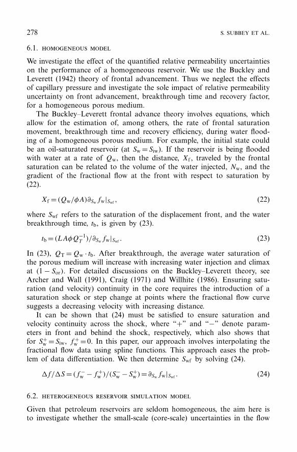
6.1. homogeneous model
We investigate the effect of the quantified relative permeability uncertaintieson the performance of a homogeneous reservoir. We use the Buckley andLeverett (1942) theory of frontal advancement. Thus we neglect the effectsof capillary pressure and investigate the sole impact of relative permeabilityuncertainty on front advancement, breakthrough time and recovery factor,for a homogeneous porous medium.
The Buckley–Leverett frontal advance theory involves equations, whichallow for the estimation of, among others, the rate of frontal saturationmovement, breakthrough time and recovery efficiency, during water flood-ing of a homogeneous porous medium. For example, the initial state couldbe an oil-saturated reservoir (at Sw =Siw). If the reservoir is being floodedwith water at a rate of Qw, then the distance, Xf , traveled by the frontalsaturation can be related to the volume of the water injected, Nw, and thegradient of the fractional flow at the front with respect to saturation by(22).
Xf = (Qw/φA)∂Swfw|Swf , (22)
where Swf refers to the saturation of the displacement front, and the waterbreakthrough time, tb, is given by (23).
tb = (LAφQ−1T )/∂Swfw|Swf . (23)
In (23), QT =Qw · tb. After breakthrough, the average water saturation ofthe porous medium will increase with increasing water injection and climaxat (1 − Sor). For detailed discussions on the Buckley–Leverett theory, seeArcher and Wall (1991), Craig (1971) and Willhite (1986). Ensuring satu-ration (and velocity) continuity in the core requires the introduction of asaturation shock or step change at points where the fractional flow curvesuggests a decreasing velocity with increasing distance.
It can be shown that (24) must be satisfied to ensure saturation andvelocity continuity across the shock, where “+” and “−” denote param-eters in front and behind the shock, respectively, which also shows thatfor S+
w =Siw, f +w =0. In this paper, our approach involves interpolating the
fractional flow data using spline functions. This approach eases the prob-lem of data differentiation. We then determine Swf by solving (24).
�f/�S= (f −w −f +
w )/(S−w −S+
w )= ∂Swfw|Swf . (24)
6.2. heterogeneous reservoir simulation model
Given that petroleum reservoirs are seldom homogeneous, the aim here isto investigate whether the small-scale (core-scale) uncertainties in the flow
QUANTIFYING UNCERTAINTY IN FLOW FUNCTIONS 279
functions could have significant impact on important heterogeneous reser-voir parameters. For this particular case, the truth corresponds to the res-ervoir model with the true (error-free) relative permeability and capillarypressure curves. The aim is to investigate to what degree the uncertaintiesin the flow functions affect, e.g., the oil recovery efficiency of the reservoir.
The original fine grid is a geostatistical model. It is represented in athree-dimensional domain [(x, y), z] ∈ R2 × R, being [1200 × 2200 × 170]feet3, and discretized into [60 × 220 × 85] cells. The model consists of twodistinct geological formations. For a full description of the model as wellas details of the fluid properties, see Floris et al., (1999) and Christie andBlunt (2001).
We generated a coarser grid model consisting of 5 × 11 × 10 grid cells,using single phase upscaling of the fine grid (Christie, 1996). There are fourproducers in the four corners of the model (P1 −P4) and a central injec-tor (I1). All wells are vertical and penetrate up to the eighth layer of thevertical column.
In Christie and Blunt (2001), the rock curves consisted of a single pairof oil–water relative permeability curves with zero capillary pressure. Wefollow the same approach and represent the rock curves by a single setof oil–water relative permeability curves but include capillary pressure. Thetrue heterogeneous model corresponds to running the coarse grid modelwith the true (error-free) set of flow functions. The ensemble of coarse gridsolutions was obtained based on the ensemble of generated (sampled) flowfunctions.
A more rigorous approach will be to use flow functions generated byhistory-matching data generated by using heterogeneous cores, and includ-ing multiple flow regions. Indeed, there are several possible extensions ofthis methodology. However, this is beyond the scope of this paper.
7. Results and Discussions
We generated 1000 models by sampling a 13-parameter space; 4 parameterseach for the oil and water relative permeability functions and 5 parametersfor the capillary pressure function. These parameters are the spline coeffi-cients. Unless otherwise stated, the units for capillary pressure curves willbe in atmospheres.
Figure 2(a) shows a plot of the model misfit as a function of modelindex. The graph shows how the NA algorithm slowly adapts the sam-pling to low misfit regions of the parameter space. Figure 2(b)–(d) show thefunctions generated for the capillary pressure, water, and oil relative perme-ability functions, respectively.
The accuracy of the maximum likelihood model could also be observedin the way it predicts the in-phase flow functions in Figure 3(a) and (b).
280 S. SUBBEY ET AL.
0 200 400 600 800 100020
40
60
80
100
120
140
model index
mis
fit
0.2 0.4 0.6 0.8 10
0.1
0.2
0.3
0.4
0.5
S
Pc
Misfit values Sampled Pc functions
0.2 0.4 0.6 0.8 10
0.1
0.2
0.3
0.4
S
Krw
0.2 0.4 0.6 0.8 10
0.2
0.4
0.6
0.8
1
S
Kro
Sampled Krw functions Sampled Kro functions
(a) (b)
(c) (d)
Figure 2. Sampling results.
0.2 0.4 0.6 0.8 10
0.1
0.2
0.3
0.4
S
Pc ml
truth
0.2 0.4 0.6 0.8 10
0.2
0.4
0.6
0.8
1
truthmltruthml K
rw
Kro
Capillary pressure function Relative permeability functions
(a) (b)
Figure 3. Maximum likelihood model performance.
QUANTIFYING UNCERTAINTY IN FLOW FUNCTIONS 281
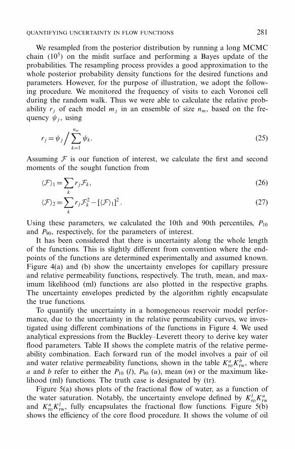
We resampled from the posterior distribution by running a long MCMCchain (105) on the misfit surface and performing a Bayes update of theprobabilities. The resampling process provides a good approximation to thewhole posterior probability density functions for the desired functions andparameters. However, for the purpose of illustration, we adopt the follow-ing procedure. We monitored the frequency of visits to each Voronoi cellduring the random walk. Thus we were able to calculate the relative prob-ability rj of each model mj in an ensemble of size nm, based on the fre-quency ψj , using
rj =ψj/ nm∑
k=1
ψk. (25)
Assuming F is our function of interest, we calculate the first and secondmoments of the sought function from
〈F〉1 =∑
k
rjFk, (26)
〈F〉2 =∑
k
rjF2k − [〈F〉1]2 . (27)
Using these parameters, we calculated the 10th and 90th percentiles, P10
and P90, respectively, for the parameters of interest.It has been considered that there is uncertainty along the whole length
of the functions. This is slightly different from convention where the end-points of the functions are determined experimentally and assumed known.Figure 4(a) and (b) show the uncertainty envelopes for capillary pressureand relative permeability functions, respectively. The truth, mean, and max-imum likelihood (ml) functions are also plotted in the respective graphs.The uncertainty envelopes predicted by the algorithm rightly encapsulatethe true functions.
To quantify the uncertainty in a homogeneous reservoir model perfor-mance, due to the uncertainty in the relative permeability curves, we inves-tigated using different combinations of the functions in Figure 4. We usedanalytical expressions from the Buckley–Leverett theory to derive key waterflood parameters. Table II shows the complete matrix of the relative perme-ability combination. Each forward run of the model involves a pair of oiland water relative permeability functions, shown in the table Ka
roKbrw, where
a and b refer to either the P10 (l), P90 (u), mean (m) or the maximum like-lihood (ml) functions. The truth case is designated by (tr).
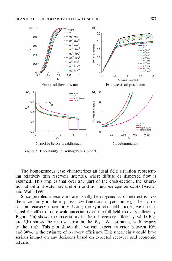
Figure 5(a) shows plots of the fractional flow of water, as a function ofthe water saturation. Notably, the uncertainty envelope defined by Kl
roKurw
and KuroK
lrw, fully encapsulates the fractional flow functions. Figure 5(b)
shows the efficiency of the core flood procedure. It shows the volume of oil
282 S. SUBBEY ET AL.
0.2 0.4 0.6 0.8 10
0.1
0.2
0.3
0.4
0.5
0.6
S
Pc
truthP
10meanP
90ml
0.2 0.4 0.6 0.8 10
0.2
0.4
0.6
0.8
1
S
truthP
10meanP
90ml
Krw
Kro
Pc uncertainty Krj uncertainty
(a) (b)
Figure 4. Uncertainty in flow functions.
Table II. Model matrix
KlroK
lrwK
lroK
lrw Kl
roKmrwK
mroK
mrw Kl
roKurwK
mroK
urwK
uroK
urw
KuroK
lrwK
mlro K
mlrw Ku
roKmrwK
trroK
trrw
produced as a function of the volume of water injected, quantified in termsof the pore volume (PV) of the porous medium. Figure 5(b) shows thatthe apparently narrow uncertainty in the relative permeability curves, leadsto an uncertainty of about 10% pore volumes in the prediction of recov-erable oil during water flooding. This, in real field terms, can lead to highuncertainty in any decisions, which depend on an estimate of the recoveryefficiency, e.g., enhanced oil recovery strategies, economic and managerialdecisions.
Figure 5(c) shows the water saturation profile as a function of the distancefrom the water injection end, before the water breakthrough. It also indi-cates the shock height for the truth, maximum likelihood (ml), Kl
roKurw (upper
bound) and KuroK
lrw (lower bound). We note here that the bound defined
by the lower and upper bounds rightly encapsulate the truth and maximumlikelihood behavior. In terms of real field simulation, the information in Fig-ure 5(a) and (c) give indications to the possible sweep efficiency of a plannedwater flood project.
Figure 5(d) gives explicit information about how much residual oil isto be expected during water flooding of the porous medium. For a givenpore volume of injected water, one can determine the water saturation to beexpected and therefore the corresponding residual oil saturation. This fig-ure shows that there is a large degree of uncertainty in the expected resid-ual oil saturation. In summary, the maximum likelihood model appears tobe highly accurate in predicting the truth.
QUANTIFYING UNCERTAINTY IN FLOW FUNCTIONS 283
0.2 0.4 0.6 0.8 10
0.2
0.4
0.6
0.8
1
S
f wtruthmlkrol krwl
krol krwm
krol krwu
krom krwl
krom krwm
krom krwu
krou krwl
krou krwm
krou krwu
0 0.5 1 1.5 20
0.1
0.2
0.3
0.4
0.5
PV water injected
PV
oil
prod
uced truth
mlkrol krwl
krol krwm
krol krwu
krom krwl
krom krwm
krom krwu
krou krwl
krou krwm
krou krwu
Fractional flow of water Estimate of oil production
0 1 2 3 40.2
0.4
0.6
0.8
1
Xf
Sw
truthmlupper boundlower bound
1 Sor
0.5 0.55 0.6 0.650
0.5
1
1.5
2
S
PV
wat
er in
ject
ed
truthmlupper boundlower bound
Sw profile before breakthrough Sor determination
(a) (b)
(c) (d)
Figure 5. Uncertainty in homogeneous model.
The homogeneous case characterizes an ideal field situation represent-ing relatively thin reservoir intervals, where diffuse or dispersed flow isassumed. This implies that over any part of the cross-section, the satura-tion of oil and water are uniform and no fluid segregation exists (Archerand Wall, 1991).
Since petroleum reservoirs are usually heterogeneous, of interest is howthe uncertainty in the in-phase flow functions impact on, e.g., the hydro-carbon recovery uncertainty. Using the synthetic field model, we investi-gated the effect of core scale uncertainty on the full field recovery efficiency.Figure 6(a) shows the uncertainty in the oil recovery efficiency, while Fig-ure 6(b) shows the relative error in the P10 − P90 estimates, with respectto the truth. This plot shows that we can expect an error between 10%and 30%, in the estimate of recovery efficiency. This uncertainty could haveserious impact on any decisions based on expected recovery and economicreturns.
284 S. SUBBEY ET AL.
0 1000 2000 3000 40000
0.05
0.1
0.15
0.2
0.25
0.3
0.35
Time (days)
Fie
ld o
il re
cove
ry e
ffici
ency
truthP
10meanP
90ml
0 1000 2000 3000 4000 –0.2
–0.1
0
0.1
0.2
0.3
0.4
0.5
Time(days)
Rel
ativ
e er
ror
P10
P90
Recovery effciency Relative error in recovery effciency
(a) (b)
Figure 6. Uncertainty in recovery efficiency – heterogeneous model.
8. Summary and Conclusions
Using synthetic data, we have demonstrated a method for deriving relativepermeability and capillary pressure functions from uncertain, unsteady-statelaboratory data. Our approach involves generating multiple flow functions,which can reproduce the experimental data within some tolerance. We haveused the NA algorithm in generating the family of solutions and shownhow an error bound, which captures the truth, could be generated, by re-sampling from the posterior distribution.
Results presented in this paper show that the use of rigid analyti-cal representation of the in-phase flow functions could introduce furtheruncertainty in the derived flow functions. The use of flexible functions,capable of capturing local effects, e.g., splines functions or Bernstein poly-nomials, is a viable alternative. Using normalized B-spline basis functionsimplies that for n model parameters the parameter space is confined to liewithin an n-dimensional cuboid, thus eliminating the problem of rescalingthe parameter space. In history matching models with high throughput, thisapproach of restricting the parameter space to regions, which contain phys-ically acceptable solutions, is desirable.
We have investigated the impact of the uncertainty in the flow functionon the oil recovery efficiency of two types of synthetic reservoir models.For this particular example, our results indicate that the core scale uncer-tainties have significant impact on the performance of both homogeneousand heterogeneous reservoirs.
Our results, however, are dependent on the definition of the performanceindex, which quantifies the misfit surface. In this, paper, we have madenon-rigorous estimates of the data correlation and variance. A future paperwill address this issue using a more rigorous approach.
QUANTIFYING UNCERTAINTY IN FLOW FUNCTIONS 285
Acknowledgements
The authors are grateful to the sponsors (Anadarko, BG, BP, ConocoPhillips,DTI, ENI, JNOC, Landmark, Shell and Statoil) of the Uncertainty and Up-scaling research at Heriot-Watt University for funding. We are also gratefulto Schlumberger-GeoQuest for the use of the Eclipse simulator.
References
Akin, S., Castanier, L. M. and Brigham, W. E.: 1999, Effect of temperature on heavyoil/water relative permeabilities, Soc. Petrol. Eng. J. 54120, 1–11.
Archer, J. S. and Wall, P. G.: 1991, Petroleum Engineering: Principles and Practice, Graham& Trotman, London.
Archer, J. S. and Wong, S. W.: 1973, Use of a reservoir simulator to interpret laboratorywaterflood data, Soc. Petrol. Eng J. 3551, 343–347.
Buckley, S. E. and Leverett, M. C.: 1942, Mechanisms of fluid displacement in sands, Trans.Am. Inst. Min. Eng. 146, 107–116.
Chavent, G., Cohen, G. and Espy, M.: 1980, Determination of relative permeabilities andcapillary pressures by an automatic adjustment method, Soc. Petrol. Eng. 9237, 1–10.
Chierici, G. L.: 1981, Novel relations for drainage and imbibition relative permeabilities. Soc.Petrol. Eng. 10165, 1–10.
Christie, M. A.: 1996, Upscaling for reservoir simulation, Soc. Petrol. Eng. 37324, 1–5.Christie, M. A. and Blunt, M. J.: 2001, Tenth SPE Comparative Solution Project: a com-
parison of upscaling techniques, Soc. Petrol. Eng. 66599, 1–9.Civan, F. and Donaldson, E. C.: 1987, Relative permeability from unsteady-state displace-
ments: an analytical interpretation, Soc. Petrol. Eng. 16200, 139–155.Civan, F. and Donaldson, E. C.: 1989, Relative permeability from unsteady-state displace-
ments with capillary pressure included, SPE Form. Eval. (June) 189–193.Collins, E. R.: 1976, Flow of Fluids through Porous Materials, PennWell Books, Tulsa,
Oklahoma.Corey. A. T.:1954, The Interrelation between gas and oil permeabilities, Producers Monthly
19, 38–41.Craig, F. F. Jr.: 1971, The Reservoir Engineering Aspects of Waterflooding, Society of Petro-
leum Engineers of AIME, New York.Floris, F. J. T., Bush, M. D., Cuypers, M., Roggero, F. and Syversveen, A. R.: 1999, Com-
parison of production forecast uncertainty quantification methods – an integrated study,in: Proceedings of 1st Conference on Petroleum Geostatistics, Toulouse, France, pp. 1–20.
Gabbanelli, S. C., Mezzatesta, A. G. and Bidner, M. S.: 1982, One-dimensional numericalsimulation of waterflooding an oil reservoir. Lat. Am. J. Heat Mass. Transf. 6, 251–273.
Geman, S. and Geman, D.: 1984, Stochastic relaxation, Gibbs distributions and the Bayesianrestoration of images, IEEE Trans. Pattern Anal. Mach. Int. 6, 721–741.
Gill, P. E. and Murray, W.: 1981, Practical Optimization, Academic Press, New York City.Glimm, J., Hou, S., Lee, Y. H., Sharp, D. and Ye, K.: 2001, Prediction of oil preduction
with confidence intervals. Soc. Petrol. Eng. 66350, 1–15.Glimm, J. Hou, S. Kim, H. and Sharp, D. H.: 2001, A probability model for errors in the
numerical solutions of a partial differential equation, Fluid Dyn. J. 9, 485–493.Grattoni, C. A. and Bidner, M. S.: 1990, History matching of unsteady-state corefloods for
Hansen, K. M., Cunningham, G. S. and McKee, R. J.: 1977, Uncertainty assessment forreconstruction based on deformable geometry, Int. J. Imag. Syst. Technol. 8, 506–512.
Honarpour, M., Koederitz, L. and Harvey, A. H.: 1986, Relative Permeability of PetroleumReservoirs, CRC Press, Inc., Boca Raton, Florida.
Johnson, E. F., Bossler, D. P. and Naumann, V. O.: 1959, Calculation of relative permeabilityfrom displacement experiments, Trans. Am. Inst. Min. Eng. 216, 370–372.
Kerig, P. D. and Watson, A. T.: 1987, A new algorithm for estimating relative permeabilitiesfrom displacement experiments, Soc. Petrol. Eng. Reserv. Eval. 2(1), 103–112.
MacMillan, D. J.: 1987, Automatic history matching of laboratory corefloods to obtain rel-ative-permeability curves, Soc. Petrol. Eng. Reserv. Eval. 2(1), 85–91.
Marle, C. M.: 1981, Multiphase Flow in Porous Media, Gulf Pub. Co., Texas.Osoba, J. S., Richardson, J. G., Kerver, J. K., Hafford, J. A. and Blair, P. M.: 1951, Labo-
ratory measurements of relative permeability, Trans. Am. Ins. Min. Eng. 192, 47–56.Richardson, J. G., Kerver, J. K., Hafford, J. A. and Osoba, J. S.: 1952, Laboratory determi-
nation of relative permeability, Trans. Am. Inst. Min. Eng. 195, 187–196.Richmond, P. C. and Watson. A. T.: 1990, Estimation of multiphase flow functions from
displacement experiments, Soc. Reserv. Eng. 18569, 1–7.Sambridge, M.: 1998, Exploring multidimensional landscapes without a map, Inverse Probl.
14, 427–440.Sambridge, M.: 1999, Geophysical inversion with a neighbourhood algorithm – 1. Searching
a parameter space, Geophys. J. Int. 138 479–494.Sambridge, M.: 1999, Geophysical inversion with a neighbourhood algorithm – II. Apprais-
ing the ensemble, Geophys. J. Int. 138, 727–745.Savioli, G. B. and Bidner, M. S.: 1982, The influence of capillary pressure when determining
relative permeability from unsteady-state corefloods, Soc. Petrol. Eng. 23698, 1–10.Schumaker, L. L.: 1981, Spline Functions: Basic Theory, John Wiley & Sons, New York.Sigmund, P. M. and McCaffery, F. G.: 1979, An improved unsteady-state procedure for
determining the relative-permeability characteristics of heterogeneous porous media, Soc.Petrol. Eng. J. 6720, 1–14.
Sivia, D. S.: 1996, Data Analysis – A Bayesian Tutorial. Clarendon Press, Oxford.Subbey, S.: 2000, Regularizing the Volterra Integral Equation – the Capillary Pressure Case.
PhD thesis, University of Bergen, Norway.Subbey, S., Christie, M. and Sambridge, M.: 2002a, A strategy for rapid quantification of
uncertainty in reservoir performance prediction, Soc. Petrol. Eng. 79678, 1–12.Subbey, S., Christie, M. and Sambridge, M.: 2002b, Uncertainty reduction in reservoir mod-
eling, SIAM Contemp. Math. 295, 457–467.Subbey, S. Christie, M. and Sambridge, M.: 2004, The impact of uncertain centrifuge capil-
lary pressure on reservoir simulation, SIAM J. Sci. Comput. 26(2), 537–557.Tao, T. M. and Watson, A. T.: 1984, Accuracy of JBN estimates of relative permeability:
part 1 – error analysis. SPEJ (April) 209–214.Tao, T. M. and Watson, A. T.: (1984), Accuracy of JBN estimates of relative permeability:
part 2 – algorithms. SPEJ (April) 215–223.Tarantola, A.: 1987, Inverse Problem Theory, Methods for Data Fitting and Model Parameter
Estimation, Elsevier Science Publishers, Amsterdam, The Netherlands.Watson, A. T., Kulkarni, R., Nordtvedt, J.-E., Sylte, A. and Urkedal, H.: 1998, Estimation
of porous media flow functions, Meas. Sci. Technol. 9, 898–905.Welge. H. J.: 1952, A simplified method for computing oil recovery by gas or water drive,
Trans. Am. Inst. Min. Eng. 195, 91–98.Willhite, G. P.: 1986, Waterflooding, Society of Petroleum Engineers, Richardson, TX.


![Untitled-1 [rses.anu.edu.au]](https://static.documents.pub/doc/80x56/616d79e18bd91c532f64ef86/untitled-1-rsesanueduau.jpg)


