Page 1
Asymptotic Normality of Quantile Estimator
Quantile Regressions: Estimations, Asymptotic
Normality and Hypothesis Testing
MEI-YUAN CHEN
Department of Finance
National Chung Hsing University
August 13, 2016
M.-Y. Chen (NCHU) Chiang-Mai University August 13, 2016 1 / 86
Page 2
Asymptotic Normality of Quantile Estimator
Scope of Quantile Regressions
1 Cross-sectional Data:
1 Quantile regressions: wage equation
2 Censored quantile regressions
2 Time-Series Data:
1 Qauntile regressions for non-causality test
2 Quantile regressions with breaks
3 Quantile autoregression
4 Quantile ARCH and GARCH
5 Quantile unit root and cointegration
3 Panel Data:
1 Panel quantile regressions
2 Panel censored quantile regressionsM.-Y. Chen (NCHU) Chiang-Mai University August 13, 2016 2 / 86
Page 3
Asymptotic Normality of Quantile Estimator
Why Quantile?
A univariate random variable Y is defined as
Y : Ω → y1, y2, . . . = DY (µY , var(Y ), α3(Y ), α4(Y )).
The distribution of realizations is demonstrated by measures E(Y )
(unconditional mean), var(Y ) (unconditional variance), α3(Y )
(unconditional skewness), α4(Y ) (unconditional kurtosis). Of course,
the distribution of all realizations can be captured by the cumulative
distribution function FY and the probability density function fY if FYis globally differentiable.
M.-Y. Chen (NCHU) Chiang-Mai University August 13, 2016 3 / 86
Page 4
Asymptotic Normality of Quantile Estimator
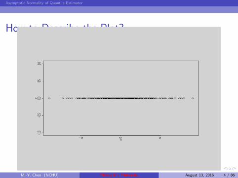
How to Describe the Plot?
−2 0 2
−1.0
−0.5
0.00.5
1.0
x
y
M.-Y. Chen (NCHU) Chiang-Mai University August 13, 2016 4 / 86
Page 5
Asymptotic Normality of Quantile Estimator
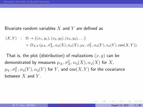
Bivariate random variables X and Y are defined as
(X,Y ) : Ω → (x1, y1), (x2, y2), (x3, y3), . . .= DX,Y (µX , σ
2X , α3(X), α4(X), µY , σ
2Y , α3(Y ), α4(Y ), cov(X,Y )).
That is, the plot (distribution) of realizations (x, y) can be
demonstrated by measures µX , σ2X , α3(X), α4(X) for X ,
µY , σ2Y , α3(Y ), α4(Y ) for Y , and cov(X, Y ) for the covariance
between X and Y .
M.-Y. Chen (NCHU) Chiang-Mai University August 13, 2016 5 / 86
Page 6
Asymptotic Normality of Quantile Estimator
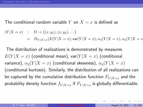
The conditional random variable Y on X = x is defined as
(Y |X = x) : Ω → (x, y1), (x, y2), . . .= DY |X=x(E(Y |X = x), var(Y |X = x), α3(Y |X = x), α4(Y |X = x))
The distribution of realizations is demonstrated by measures
E(Y |X = x) (conditional mean), var(Y |X = x) (conditional
variance), α3(Y |X = x) (conditional skewness), α4(Y |X = x)
(conditional kurtosis). Similarly, the distribution of all realizations can
be captured by the cumulative distribution function FY |X=x and the
probability density function fY |X=x if FY |X=x is globally differentiable.
M.-Y. Chen (NCHU) Chiang-Mai University August 13, 2016 6 / 86
Page 7
Asymptotic Normality of Quantile Estimator
Purpose of Exploring the Conditional Distribution
To answer whether DY |X=x = DY , i.e.,
H0 : DY |X=x = DY , ∀x ∈ R. If the answer is NOT, the
information about X is valuable to understand the disytribution
of Y .
H0 : E(Y |X = x) = E(Y ), ∀x ∈ R;
H0 : var(Y |X = x) = var(Y ), ∀x ∈ R;
H0 : α3(Y |X = x) = α3(Y ), ∀x ∈ R;
H0 : α4(Y |X = x) = α4(Y ), ∀x ∈ R;
M.-Y. Chen (NCHU) Chiang-Mai University August 13, 2016 7 / 86
Page 8
Asymptotic Normality of Quantile Estimator
How to Describe the Plot?
0.0 0.2 0.4 0.6 0.8 1.0
−10
12
34
5
x
y
M.-Y. Chen (NCHU) Chiang-Mai University August 13, 2016 8 / 86
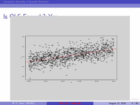
Page 9
Asymptotic Normality of Quantile Estimator
Is OLS Enough? Yes
0.0 0.2 0.4 0.6 0.8 1.0
−20
24
6
x
y
M.-Y. Chen (NCHU) Chiang-Mai University August 13, 2016 9 / 86
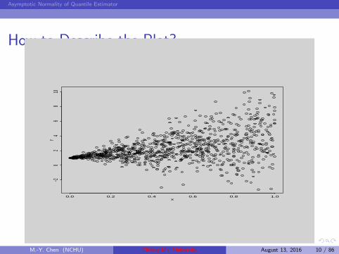
Page 10
Asymptotic Normality of Quantile Estimator
How to Describe the Plot?
0.0 0.2 0.4 0.6 0.8 1.0
−20
24
68
10
x
y
M.-Y. Chen (NCHU) Chiang-Mai University August 13, 2016 10 / 86
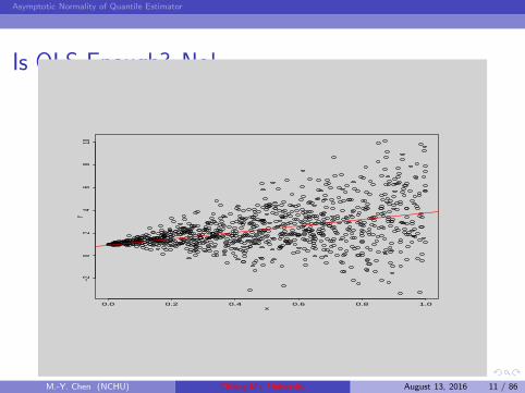
Page 11
Asymptotic Normality of Quantile Estimator
Is OLS Enough? No!
0.0 0.2 0.4 0.6 0.8 1.0
−20
24
68
10
x
y
M.-Y. Chen (NCHU) Chiang-Mai University August 13, 2016 11 / 86
Page 12
Asymptotic Normality of Quantile Estimator
Let Y denote the today’s stock return and X = 1 for having positive
and X = 0 for negative yesterday’s return. Then DY |X=x = DY
implies that knowing previous day’s return is positive or negative has
no help for understanding the distribution of today’s stock return. In
contrast, DY |X=x 6= DY indicates that knowing yesterday’s return is
positive or negative is useful to understanding the distribution of
today’s return. The information of X = 1 or X = 0 is valuable to
understand the distribution of today’s stock return. In other words,
checking DY |X=x = DY or not is equivalent to study whether the
information X is valuable or not.
M.-Y. Chen (NCHU) Chiang-Mai University August 13, 2016 12 / 86
Page 13
Asymptotic Normality of Quantile Estimator
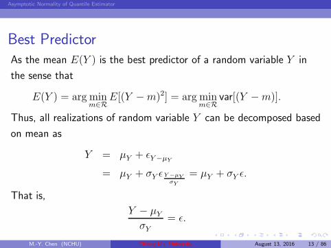
Best PredictorAs the mean E(Y ) is the best predictor of a random variable Y in
the sense that
E(Y ) = arg minm∈R
E[(Y −m)2] = arg minm∈R
var[(Y −m)].
Thus, all realizations of random variable Y can be decomposed based
on mean as
Y = µY + ǫY−µY
= µY + σY ǫY −µYσY
= µY + σY ǫ.
That is,
Y − µYσY
= ǫ.
M.-Y. Chen (NCHU) Chiang-Mai University August 13, 2016 13 / 86
Page 14
Asymptotic Normality of Quantile Estimator
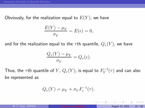
Obviously, for the realization equal to E(Y ), we have
E(Y )− µYσY
= E(ǫ) = 0,
and for the realization equal to the τ th quantile, Qτ (Y ), we have
Qτ (Y )− µYσY
= Qτ (ǫ).
Thus, the τ th quantile of Y , Qτ (Y ), is equal to F−1Y (τ) and can also
be represented as
Qτ (Y ) = µY + σY F−1ǫ (τ).
M.-Y. Chen (NCHU) Chiang-Mai University August 13, 2016 14 / 86
Page 15
Asymptotic Normality of Quantile Estimator
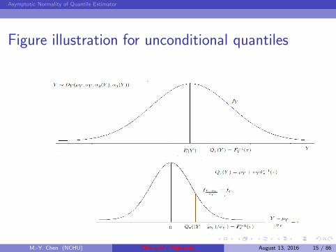
Figure illustration for unconditional quantiles
M.-Y. Chen (NCHU) Chiang-Mai University August 13, 2016 15 / 86
Page 16
Asymptotic Normality of Quantile Estimator
With no doubt that all realizations of random variable Y can also be
decomposed based on any location measure, say the first quartertile,
Q0.25(Y ), as
Y = Q0.25(Y ) + ǫ0.25
or say the third quartertile Q0.75(Y ), as
Y = Q0.75(Y ) + ǫ0.75
In general, the decomposition based on the τ th quantile can be
represented as
Y = Qτ (Y ) + ǫτ
M.-Y. Chen (NCHU) Chiang-Mai University August 13, 2016 16 / 86
Page 17
Asymptotic Normality of Quantile Estimator
Conditional Mean DecompositionSimilarly, the conditional mean E(Y |X = x) is the best predictor of the
conditional random variable (Y |X = x), i.e.,
E(Y |X = x) = arg minm∈R
E[((Y |X = x) −m)2] = arg minm∈R
var[(Y |X = x)−m].
Thus, all realizations of random variable Y conditional on X = x can be
decomposed as
(Y |X = x) = µ(Y |X=x) + ǫ(Y |X=x)−µ(Y |X=x)
= µ(Y |X=x) + σ(Y |X=x)ǫ (Y |X=x)−µ(Y |X=x)σ(Y |X=x)
= µ(Y |X=x) + σ(Y |X=x)ǫ.
That is,
(Y |X = x)− µ(Y |X=x)
σ(Y |X=x)= ǫ.
M.-Y. Chen (NCHU) Chiang-Mai University August 13, 2016 17 / 86
Page 18
Asymptotic Normality of Quantile Estimator
Obviously, for the realization equal to E(Y |X = x), we have
E(Y |X = x)− µ(Y |X=x)
σ(Y |X=x)= E(ǫ) = 0,
and for the realization equal to the τth quantile, Qτ (Y |X = x), we have
Qτ (Y |X = x)− µ(Y |X=x)
σ(Y |X=x)= Qτ (ǫ).
The τth quantile of Y |X = x, Qτ (Y |X = x), is equal to F−1(Y |X=x)(τ) and can
also be represented as
Qτ (Y |X = x) = µ(Y |X=x) + σ(Y |X=x)F−1ǫ (τ). (1)
Similarly, the realizations of (Y |X = x) can be decomposed based on the
conditional τth quantile, Qτ (Y |X = x), as
(Y |X = x) = Qτ (Y |X = x) + ǫτ .
M.-Y. Chen (NCHU) Chiang-Mai University August 13, 2016 18 / 86
Page 19
Asymptotic Normality of Quantile Estimator
Illustration for the Conditional Quantiles
M.-Y. Chen (NCHU) Chiang-Mai University August 13, 2016 19 / 86
Page 20
Asymptotic Normality of Quantile Estimator
Extend the dimension of X and k-dimension and replace the notation with X.
Taking E(Y |X = x) = x′β0 and σ(Y |X=x) = x′γ0, we have
Qτ (Y |X = x) = µ(Y |X=x) + σ(Y |X=x)F−1ǫ (τ)
= x′β0 + x′γ0F−1ǫ (τ).
Then, the decomposition of realization of Y on X = x can be represented as
(Y |X = x) = x′β0 + x′γ0F−1ǫ (τ) + ǫτ
= x′[β0 + γ0 × F−1ǫ (τ)] + ǫτ
= x′βτ + ǫτ . (2)
Since x′β0 and x′γ0 represented the location and scale of the conditional random
variable (Y |X = x), (2) is called the location-scale quantile regression model.
M.-Y. Chen (NCHU) Chiang-Mai University August 13, 2016 20 / 86
Page 21
Asymptotic Normality of Quantile Estimator
As σ(Y |X=x) = x′γ0 and let x = (1, z′)′ and γ = (γ0,γ′1)
′,
Qτ (Y |X = x) = x′β0 + x′γ0F−1ǫ (τ)
= x′β0 + (1, z′)(γ00,γ′01)
′F−1ǫ (τ)
= x′β0 + γ00F−1ǫ (τ) + z′γ01F
−1ǫ (τ).
location shift model: γ00 6= 0 and γ01 = 0;
location-scale shift model: γ00 6= 0 and γ01 6= 0.
M.-Y. Chen (NCHU) Chiang-Mai University August 13, 2016 21 / 86
Page 22
Asymptotic Normality of Quantile Estimator
Population Quantiles
Definition 3.1: For any real valued random variable, Y, distributed
according to F (y) = Prob(Y ≤ y) , while for any 0 < τ < 1,
Qτ (Y ) = infy : F (y) ≥ τ
is called the τ th quantile of Y. The population quantile τ can also be
defined as
Qτ (Y ) = β = arg minβ∈R1
E[ρτ (yt − β)],
where ρτ (u) = u(τ − I(u < 0)) is called the check function by its
shape.
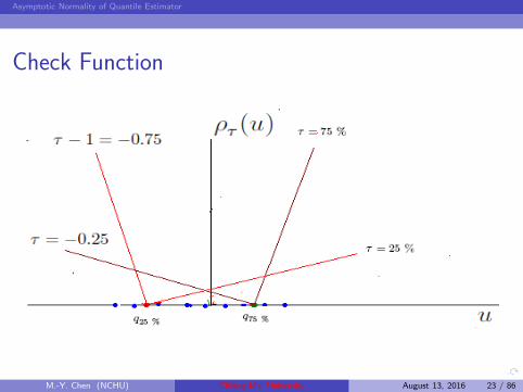
M.-Y. Chen (NCHU) Chiang-Mai University August 13, 2016 22 / 86
Page 23
Asymptotic Normality of Quantile Estimator
Check Function
M.-Y. Chen (NCHU) Chiang-Mai University August 13, 2016 23 / 86
Page 24
Asymptotic Normality of Quantile Estimator
To show why β is equivalent to the τ th population quantile, observethat
E (ρτ (yt − β)) = τ
∫
y>β
(y − β)dF (y)− (1 − τ)
∫
y<β
(y − β)dF (y). (3)
Diffrentiating (3) with respect to β and by a variant of Liebniz’s
rule: Given V (r) =∫ B(r)
A(r)f(y, r)dy, the Liebniz’s rule is stated as
V ′(r) = f(B(r), r)∂B(r)
∂r− f(A(r), r)
∂A(r)
∂r+
∫ B(r)
A(r)
∂f(y, r)
∂rdy.
M.-Y. Chen (NCHU) Chiang-Mai University August 13, 2016 24 / 86
Page 25
Asymptotic Normality of Quantile Estimator
By the Liebniz’s rule
∂
(
∫ g(x)
−∞
ψ(x, y)dy
)
/∂x =
∫ g(x)
−∞
∂ψ
∂xdy +
(
∂g
∂x
)
ψ(x, g(x)),
one gets, with g = β with y < β and ψ = y − β,
∂
(
∫ y<β
−∞
(y − β)dF (y)
)
/∂β =
∫ y<β
−∞
∂(y − β)
∂βdF (y) +
∂β
∂β(β − β)
= −∫ y<β
−∞
dF (y) + 0 = −F (y < β).
∂E (ρt(yt − β)) /∂β
= τ∂
(∫
y>β
(y − β)dF (y)
)
/∂β − (1− τ)∂
(∫
y<β
(y − β)dF (y)
)
/∂β
= τ [−F (y > β)]− (1− τ) [−F (y < β)]
= τ [−(1− F (y < β))] + (1− τ)F (y < β) = F (y < β)− τset= 0
M.-Y. Chen (NCHU) Chiang-Mai University August 13, 2016 25 / 86
Page 26
Asymptotic Normality of Quantile Estimator
Sample Quantiles
Given a sample y1, y2, . . . , yT, the sample counterpart ofE[ρτ (yt − β)] is T−1
∑Tt=1 ρτ (yt − β). Then, the sample τ th quantile
estimator is obtained by solving
Qτ(Y ) = βT = arg minβ∈R1
1
T
T∑
t=1
ρτ (yt − β)
= argminβ∈R
1
T
T∑
t=1
[τ − I(yt − β < 0)] (yt − β)
= minβ∈R
1
T
∑
t∈t:yt≥β
τ |yt − β|+∑
t∈t:yt<β
(1− τ)|yt − β|
.
M.-Y. Chen (NCHU) Chiang-Mai University August 13, 2016 26 / 86
Page 27
Asymptotic Normality of Quantile Estimator
Regression Quantiles: Koenker and Bassett (1978)Consider the τ th conditional quantile of yt on xt as
Qτ (yt|xt) = x′
tβτ .
It is ready to see
τ =
∫ x′
tβτ
−∞
fy|x(s)ds
where fy|x(·) is the conditional density function of Y on X. Then,
the τ th conditional quantile regression model can be written as
yt = x′
tβτ + ut,τ
M.-Y. Chen (NCHU) Chiang-Mai University August 13, 2016 27 / 86
Page 28
Asymptotic Normality of Quantile Estimator
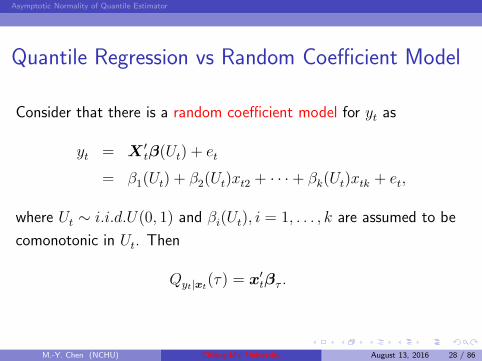
Quantile Regression vs Random Coefficient Model
Consider that there is a random coefficient model for yt as
yt = X ′tβ(Ut) + et
= β1(Ut) + β2(Ut)xt2 + · · ·+ βk(Ut)xtk + et,
where Ut ∼ i.i.d.U(0, 1) and βi(Ut), i = 1, . . . , k are assumed to be
comonotonic in Ut. Then
Qyt|xt(τ) = x′
tβτ .
M.-Y. Chen (NCHU) Chiang-Mai University August 13, 2016 28 / 86
Page 29
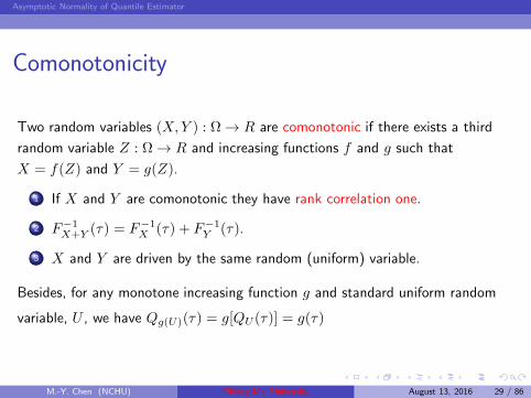
Asymptotic Normality of Quantile Estimator
Comonotonicity
Two random variables (X,Y ) : Ω → R are comonotonic if there exists a third
random variable Z : Ω → R and increasing functions f and g such that
X = f(Z) and Y = g(Z).
1 If X and Y are comonotonic they have rank correlation one.
2 F−1X+Y (τ) = F−1
X (τ) + F−1Y (τ).
3 X and Y are driven by the same random (uniform) variable.
Besides, for any monotone increasing function g and standard uniform random
variable, U , we have Qg(U)(τ) = g[QU (τ)] = g(τ)
M.-Y. Chen (NCHU) Chiang-Mai University August 13, 2016 29 / 86
Page 30
Asymptotic Normality of Quantile Estimator
Proof
Qyt|xt(τ) = Qβ1(Ut)+β2(Ut)xt2+···+βk(Ut)xtk
(τ)
= Qβ1(Ut)(τ) +Qβ2(Ut)xt2(τ) + · · ·+Qβk(Ut)xtk(τ)
= β1[QUt(τ)] + β2[QUt
(τ)]xt2 + · · ·+ βk[QUt(τ)]xtk
= β1(τ) + β2(τ)xt2 + · · ·+ βk(τ)xtk
= x′tβτ
This result holds for all τ ∈ (0, 1).
M.-Y. Chen (NCHU) Chiang-Mai University August 13, 2016 30 / 86
Page 31
Asymptotic Normality of Quantile Estimator
The point estimators βτ of the linear quantile regression parameters,βτ , are obtained by solving
βτ = arg minβ∈Rp
1
T
T∑
t=1
ρτ (yt − x′
tβ)
= arg minβ∈Rp
1
T
T∑
t=1
[
τ − I(yt − x′
tβ < 0)]
(yt − x′
tβ)
= arg minβ∈Rp
1
T
∑
t∈t:yt≥x′tβ
τ |yt − x′
tβ|+∑
t∈t:yt<x′tβ
(1− τ)|yt − x′
tβ|
.
M.-Y. Chen (NCHU) Chiang-Mai University August 13, 2016 31 / 86
Page 32
Asymptotic Normality of Quantile Estimator
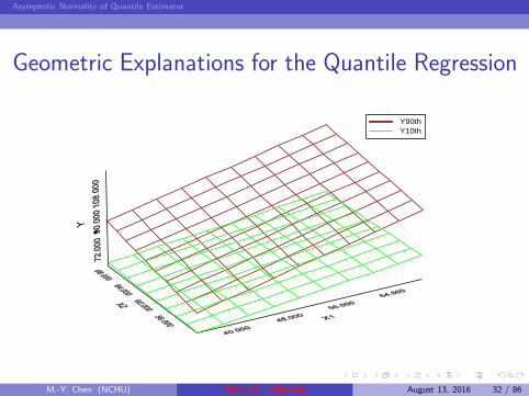
Geometric Explanations for the Quantile Regression
Y90thY10th
M.-Y. Chen (NCHU) Chiang-Mai University August 13, 2016 32 / 86
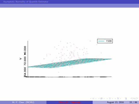
Page 33
Asymptotic Normality of Quantile Estimator
Y10th
M.-Y. Chen (NCHU) Chiang-Mai University August 13, 2016 33 / 86
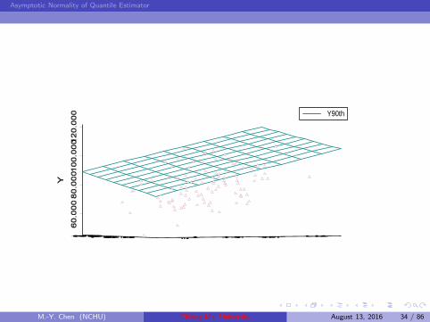
Page 34
Asymptotic Normality of Quantile Estimator
Y90th
M.-Y. Chen (NCHU) Chiang-Mai University August 13, 2016 34 / 86
Page 35
Asymptotic Normality of Quantile Estimator
Characteristics of Regression Quantiles
Robustness
Equivariant Properties: ifβ∗(τ, y,X) ∈ B∗(τ, y,X), where
B∗(τ, y,X) is the set of regression quantiles,
β∗(τ, λy,X) = λβ∗(τ, y,X), λ ∈ [0,∞),
β∗(1− τ, λy,X) = λβ∗(τ, y,X), λ ∈ (−∞, 0],
β∗(τ, y +Xγ,X) = β∗(τ, y,X) + γ, γ ∈ Rp,
β∗(τ, y,XA) = A−1β∗(τ, y,X), AP×P nonsingular.
Capability of Exploring Conditional Distributions
M.-Y. Chen (NCHU) Chiang-Mai University August 13, 2016 35 / 86
Page 36
Asymptotic Normality of Quantile Estimator
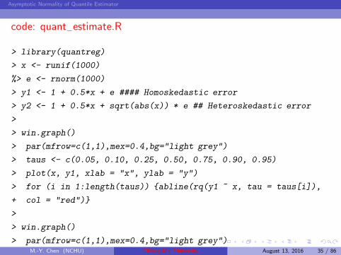
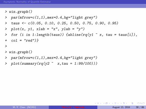
code: quant−estimate.R
> library(quantreg)
> x <- runif(1000)
%> e <- rnorm(1000)
> y1 <- 1 + 0.5*x + e #### Homoskedastic error
> y2 <- 1 + 0.5*x + sqrt(abs(x)) * e ## Heteroskedastic error
>
> win.graph()
> par(mfrow=c(1,1),mex=0.4,bg="light grey")
> taus <- c(0.05, 0.10, 0.25, 0.50, 0.75, 0.90, 0.95)
> plot(x, y1, xlab = "x", ylab = "y")
> for (i in 1:length(taus)) abline(rq(y1 ~ x, tau = taus[i]),
+ col = "red")
>
> win.graph()
> par(mfrow=c(1,1),mex=0.4,bg="light grey")M.-Y. Chen (NCHU) Chiang-Mai University August 13, 2016 35 / 86
Page 37
Asymptotic Normality of Quantile Estimator
> plot(summary(rq(y1 ~ x,tau = 1:99/100)))
M.-Y. Chen (NCHU) Chiang-Mai University August 13, 2016 36 / 86
Page 38
Asymptotic Normality of Quantile Estimator
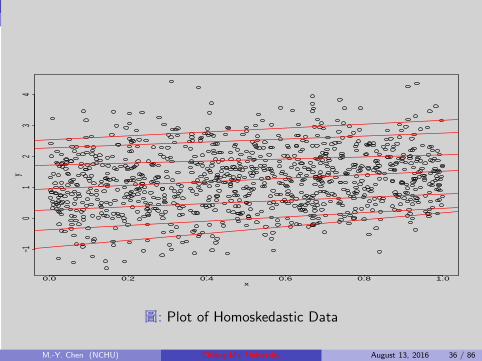
0.0 0.2 0.4 0.6 0.8 1.0
−10
12
34
x
y
圖: Plot of Homoskedastic Data
M.-Y. Chen (NCHU) Chiang-Mai University August 13, 2016 36 / 86
Page 39
Asymptotic Normality of Quantile Estimator
0.0 0.2 0.4 0.6 0.8 1.0
−2−1
01
23
4
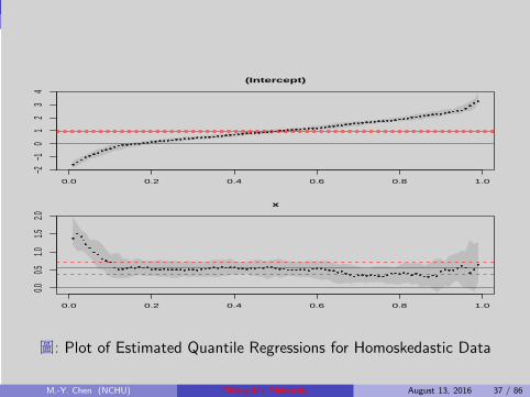
(Intercept)
0.0 0.2 0.4 0.6 0.8 1.0
0.00.5
1.01.5
2.0
x
圖: Plot of Estimated Quantile Regressions for Homoskedastic Data
M.-Y. Chen (NCHU) Chiang-Mai University August 13, 2016 37 / 86
Page 40
Asymptotic Normality of Quantile Estimator
> win.graph()
> par(mfrow=c(1,1),mex=0.4,bg="light grey")
> taus <- c(0.05, 0.10, 0.25, 0.50, 0.75, 0.90, 0.95)
> plot(x, y1, xlab = "x", ylab = "y")
> for (i in 1:length(taus)) abline(rq(y1 ~ x, tau = taus[i]),
+ col = "red")
>
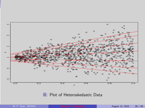
> win.graph()
> par(mfrow=c(1,1),mex=0.4,bg="light grey")
> plot(summary(rq(y2 ~ x,tau = 1:99/100)))
M.-Y. Chen (NCHU) Chiang-Mai University August 13, 2016 38 / 86
Page 41
Asymptotic Normality of Quantile Estimator
0.0 0.2 0.4 0.6 0.8 1.0
−10
12
34
x
y
圖: Plot of Heteroskedastic Data
M.-Y. Chen (NCHU) Chiang-Mai University August 13, 2016 38 / 86
Page 42
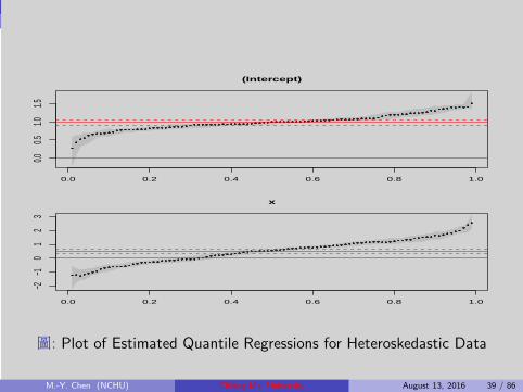
Asymptotic Normality of Quantile Estimator
0.0 0.2 0.4 0.6 0.8 1.0
0.00.5
1.01.5
(Intercept)
0.0 0.2 0.4 0.6 0.8 1.0
−2−1
01
23
x
圖: Plot of Estimated Quantile Regressions for Heteroskedastic Data
M.-Y. Chen (NCHU) Chiang-Mai University August 13, 2016 39 / 86
Page 43
Asymptotic Normality of Quantile Estimator
Quantile Regression Estimation using quantreg
Estimation methods include:
method = ”br” : The default method is the modified version of
the Barrodale and Roberts algorithm for l1-regression;
method = ”fn” : Frisch-Newton interior point method;
method =“pfn” : the Frisch-Newton approach after
preprocessing;
method =“fnc”: enables the user to specify linear inequality
constraints on the fitted coefficients;
method =“lasso” : implement the lasso penalty and Fan and Li’s
smoothly clipped absolute deviation penalty;
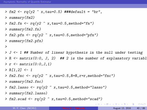
method =“scad” :M.-Y. Chen (NCHU) Chiang-Mai University August 13, 2016 40 / 86
Page 44
Asymptotic Normality of Quantile Estimator
> fm2 <- rq(y2 ~ x,tau=0.5) ###default = "br",
> summary(fm2)
> fm2.fn <- rq(y2 ~ x,tau=0.5,method="fn")
> summary(fm2.fn)
> fm2.pfn <- rq(y2 ~ x,tau=0.5,method="pfn")
> summary(fm2.pfn)
>
> J <- 1 ## Number of linear hypothesis in the null under testing
> R <- matrix(0:0, J, 2) ## 2 is the number of explanatory variables,
> r <- matrix(0:0,J,1)
> R[1,2] <- 1
> fm2.fnc <- rq(y2 ~ x,tau=0.5,R=R,r=r,method="fnc")
> summary(fm2.fnc)
> fm2.lasso <- rq(y2 ~ x,tau=0.5,method="lasso")
> summary(fm2.lasso)
> fm2.scad <- rq(y2 ~ x,tau=0.5,method="scad")
M.-Y. Chen (NCHU) Chiang-Mai University August 13, 2016 40 / 86
Page 45
Asymptotic Normality of Quantile Estimator
> summary(fm2.scad)
M.-Y. Chen (NCHU) Chiang-Mai University August 13, 2016 41 / 86
Page 46
Asymptotic Normality of Quantile Estimator
Asymptotic Normality of the LS EstimatorGiven a linear regression model yt = x′
tβ + ǫt, t = 1, . . . , T . The first order
conditions for least squares estimator, βT , are
T−1∑T
t=1(yt − x′
tβT )xt ≡ ψβT
= 0. Taking first order Taylor expansion on
ψβT
= 0 around the true parameter vector β0,
ψβT
= ψβ0+ ψ
′
β(βT − β0) +
1
2ψ′′β(βT − β0)
2 + · · ·
=1
T
[
T∑
t=1
(yt − x′
tβ0)xt −T∑
t=1
xtx′
t(βT − β0)
]
= 0
=1
T
[
T∑
t=1
xtǫt −T∑
t=1
xtx′
t(βT − β0)
]
= 0,
since ψ′ = −∑Tt−1 xtx
′t, ψ
′′ = 0, and where β equals to aβT + (1− a)β0 with
a ∈ [0, 1].
M.-Y. Chen (NCHU) Chiang-Mai University August 13, 2016 41 / 86
Page 47
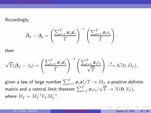
Asymptotic Normality of Quantile Estimator
Accordingly,
βT − β0 =
(
∑Tt=1 xtx
′
t
T
)−1(∑T
t=1 xtǫtT
)
,
then
√T (βT − β0) =
(
∑Tt=1 xtx
′
t
T
)−1(∑T
t=1 xtǫt√T
)
d−→ N (0, DT ),
given a law of large number∑T
t=1 xtx′t/T →MT a positive definite
matrix and a central limit theorem∑T
t=1 xtǫt/√T → N(0, VT ),
where DT =M−1T VTM
−1T .
M.-Y. Chen (NCHU) Chiang-Mai University August 13, 2016 42 / 86
Page 48
Asymptotic Normality of Quantile Estimator
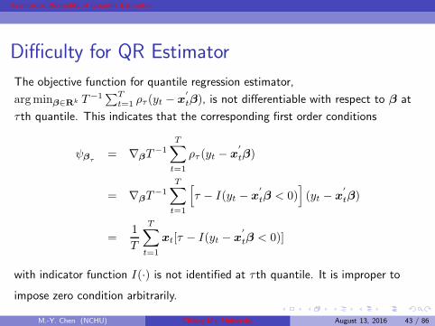
Difficulty for QR Estimator
The objective function for quantile regression estimator,
argminβ∈Rk T−1∑T
t=1 ρτ (yt − x′
tβ), is not differentiable with respect to β at
τth quantile. This indicates that the corresponding first order conditions
ψβτ= ∇βT
−1T∑
t=1
ρτ (yt − x′
tβ)
= ∇βT−1
T∑
t=1
[
τ − I(yt − x′
tβ < 0)]
(yt − x′
tβ)
=1
T
T∑
t=1
xt[τ − I(yt − x′
tβ < 0)]
with indicator function I(·) is not identified at τth quantile. It is improper to
impose zero condition arbitrarily.
M.-Y. Chen (NCHU) Chiang-Mai University August 13, 2016 43 / 86
Page 49
Asymptotic Normality of Quantile Estimator
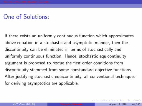
One of Solutions:
If there exists an uniformly continuous function which approximates
above equation in a stochastic and asymptotic manner, then the
discontinuity can be eliminated in terms of stochastically and
uniformly continuous function. Hence, stochastic equicontinuity
argument is proposed to rescue the first order conditions from
discontinuity stemmed from some nonstandard objective functions.
After justifying stochastic equicontinuity, all conventional techniques
for deriving asymptotics are applicable.
M.-Y. Chen (NCHU) Chiang-Mai University August 13, 2016 44 / 86
Page 50
Asymptotic Normality of Quantile Estimator
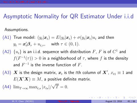
Asymptotic Normality for QR Estimator Under i.i.d
Assumptions.
(A1) True model: (yt|xt) = E(yt|xt) + σ(yt|xt)ut and then
yt = x′tβτ + ut,τ , with τ ∈ (0, 1).
(A2) ut is an i.i.d. sequence with distribution F , F is of C1 and
f(F−1(τ)) > 0 in a neighborhood of τ , where f is the density
and F−1 is the inverse function of F .
(A3) X is the design matrix, xt is the tth column of X ′, xt1 ≡ 1 and
E(X ′X) ≡M , a positive definite matrix.
(A4) limT→∞maxt,s |xts|/√T = 0.
M.-Y. Chen (NCHU) Chiang-Mai University August 13, 2016 45 / 86
Page 51
Asymptotic Normality of Quantile Estimator
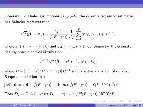
Theorem 5.2: Under assumptions (A1)-(A4), the quantile regression estimator
has Bahadur representation
√T (βτ − βτ ) =
M−1
f(F−1(τ))
1√T
T∑
t=1
xtψτ (ut,τ ) + op(1),
where ψτ (·) = τ − I(· < 0) and ψβ(·) ≡ xtψτ (·). Consequently, the estimator
has asymptotic normal distribution
D−1/2√T (βτ − βτ )
d−→ N (0, Ik) .
where D = [τ(1 − τ)/f2(F−1(τ))]M−1 and Ik is the k × k identity matrix.
Suppose in addition that
(A5) there exists f(F−1(τ)) such that f(F−1(τ)) − f(F−1(τ))p→ 0.
Then DT −Dp→ 0, where DT = [τ(1 − τ)/f2(F−1(τ))](X ′X/T )−1.
M.-Y. Chen (NCHU) Chiang-Mai University August 13, 2016 46 / 86
Page 52
Asymptotic Normality of Quantile Estimator
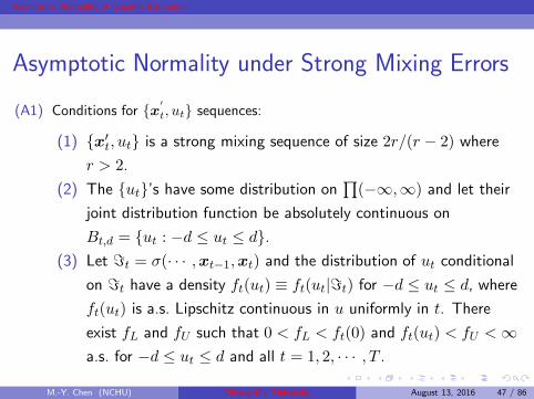
Asymptotic Normality under Strong Mixing Errors
(A1) Conditions for x′
t, ut sequences:
(1) x′t, ut is a strong mixing sequence of size 2r/(r − 2) where
r > 2.
(2) The ut’s have some distribution on∏
(−∞,∞) and let their
joint distribution function be absolutely continuous on
Bt,d = ut : −d ≤ ut ≤ d.(3) Let ℑt = σ(· · · ,xt−1,xt) and the distribution of ut conditional
on ℑt have a density ft(ut) ≡ ft(ut|ℑt) for −d ≤ ut ≤ d, where
ft(ut) is a.s. Lipschitz continuous in u uniformly in t. There
exist fL and fU such that 0 < fL < ft(0) and ft(ut) < fU <∞a.s. for −d ≤ ut ≤ d and all t = 1, 2, · · · , T .
M.-Y. Chen (NCHU) Chiang-Mai University August 13, 2016 47 / 86
Page 53
Asymptotic Normality of Quantile Estimator
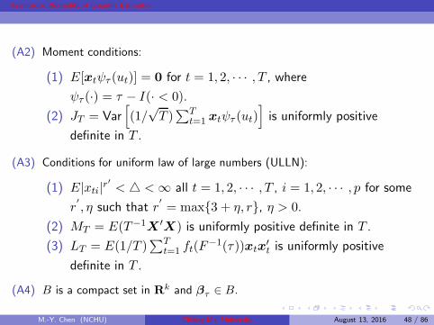
(A2) Moment conditions:
(1) E[xtψτ (ut)] = 0 for t = 1, 2, · · · , T , whereψτ (·) = τ − I(· < 0).
(2) JT = Var[
(1/√T )∑T
t=1 xtψτ (ut)]
is uniformly positive
definite in T .
(A3) Conditions for uniform law of large numbers (ULLN):
(1) E|xti|r′
< <∞ all t = 1, 2, · · · , T , i = 1, 2, · · · , p for some
r′
, η such that r′
= max3 + η, r, η > 0.
(2) MT = E(T−1X ′X) is uniformly positive definite in T .
(3) LT = E(1/T )∑T
t=1 ft(F−1(τ))xtx
′t is uniformly positive
definite in T .
(A4) B is a compact set in Rk and βτ ∈ B.
M.-Y. Chen (NCHU) Chiang-Mai University August 13, 2016 48 / 86
Page 54
Asymptotic Normality of Quantile Estimator
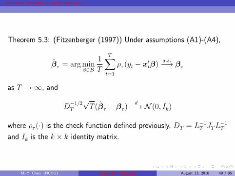
Theorem 5.3: (Fitzenberger (1997)) Under assumptions (A1)-(A4),
βτ = argminβ∈B
1
T
T∑
t=1
ρτ (yt − x′tβ)
a.s.−→ βτ
as T → ∞, and
D−1/2T
√T (βτ − βτ )
d−→ N (0, Ik)
where ρτ (·) is the check function defined previously, DT = L−1T JTL
−1T
and Ik is the k × k identity matrix.
M.-Y. Chen (NCHU) Chiang-Mai University August 13, 2016 49 / 86
Page 55
Asymptotic Normality of Quantile Estimator
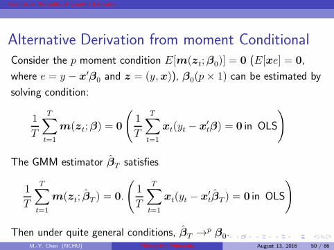
Alternative Derivation from moment ConditionalConsider the p moment condition E[m(zt;β0)] = 0 (E[xe] = 0,
where e = y − x′β0 and z = (y,x)), β0(p× 1) can be estimated by
solving condition:
1
T
T∑
t=1
m(zt;β) = 0
(
1
T
T∑
t=1
xt(yt − x′tβ) = 0 in OLS
)
The GMM estimator βT satisfies
1
T
T∑
t=1
m(zt; βT ) = 0.
(
1
T
T∑
t=1
xt(yt − x′tβT ) = 0 in OLS
)
Then under quite general conditions, βT →p β0.M.-Y. Chen (NCHU) Chiang-Mai University August 13, 2016 50 / 86
Page 56
Asymptotic Normality of Quantile Estimator
Suppose that the following uniform law of large number is satisfied,
1
T
T∑
t=1
∇βm(zt; βT ) →p G0 := E[∇βm(zt;β0)],
−1
T
T∑
t=1
∇βxt(yt − x′tβT ) =
1
T
T∑
t=1
xtx′t →p G0 :=
1
T
T∑
t=1
E(xtx′t) in OLS
where G0 is nonsingular. Then, it can be shown that
√T (βT − β0) → N (0,G−1
0 Σ0G−10 ), (4)
where Σ0 = E[m(zt;β0)m(zt;β0)′] = var[m(zt,β0)] (is
E[xte2tx
′t] = var(xtet) in OLS).
M.-Y. Chen (NCHU) Chiang-Mai University August 13, 2016 51 / 86
Page 57
Asymptotic Normality of Quantile Estimator
Ignoring the observations that yt = x′tβ (since the first derivative of
the objection is not identified), we can write the approximate, first
order condition of minimization is
1
T
T∑
t=1
ψβτ(yt − x′
tβ) =1
T
T∑
t=1
xt[τ − 1yt−x′
tβ<0] = op(1). (5)
M.-Y. Chen (NCHU) Chiang-Mai University August 13, 2016 52 / 86
Page 58
Asymptotic Normality of Quantile Estimator
Assume that (yt,x′t)
′ are i.i.d. random vectors. Taking expectation of
(5) and given
E(1yt−x′
tβ<0|xt) = Fy|x(x′tβ),
we have
E
(
1
T
T∑
t=1
[ψβτ(yt − x′
tβ)]
)
= E[ψβτ(yt − x′
tβ)] = E[xt[τ − 1yt−x′
tβ<0]]
= Ext[τ −E(1yt−x′
tβ<0|xt)] = Ext[τ − Fy|x(x′tβ)].
As Fy|x(x′tβτ ) = τ , the moment condition is hold since
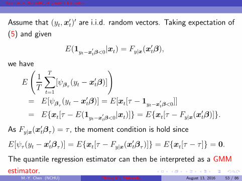
E[ψτ (yt − x′tβτ )] = Ext[τ − Fy|x(x
′tβτ )] = Ext[τ − τ ] = 0.
The quantile regression estimator can then be interpreted as a GMM
estimator.M.-Y. Chen (NCHU) Chiang-Mai University August 13, 2016 53 / 86
Page 59
Asymptotic Normality of Quantile Estimator
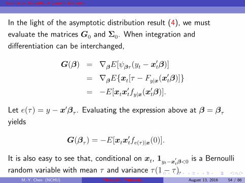
In the light of the asymptotic distribution result (4), we must
evaluate the matrices G0 and Σ0. When integration and
differentiation can be interchanged,
G(β) = ∇βE[ψβτ (yt − x′tβ)]
= ∇βExt[τ − Fy|x(x′tβ)]
= −E[xtx′tfy|x(x
′tβ)].
Let e(τ) = y − x′βτ . Evaluating the expression above at β = βτ
yields
G(βτ ) = −E[xtx′tfe(τ)|x(0)].
It is also easy to see that, conditional on xt, 1yt−x′
tβ<0 is a Bernoulli
random variable with mean τ and variance τ(1− τ).M.-Y. Chen (NCHU) Chiang-Mai University August 13, 2016 54 / 86
Page 60
Asymptotic Normality of Quantile Estimator
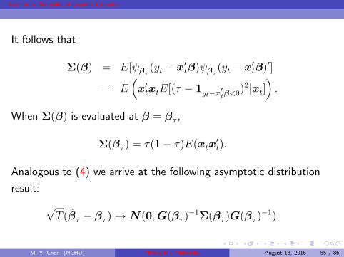
It follows that
Σ(β) = E[ψβτ(yt − x′
tβ)ψβτ(yt − x′
tβ)′]
= E(
x′txtE[(τ − 1yt−x
′
tβ<0)2|xt]
)
.
When Σ(β) is evaluated at β = βτ ,
Σ(βτ ) = τ(1 − τ)E(xtx′t).
Analogous to (4) we arrive at the following asymptotic distribution
result:
√T (βτ − βτ ) → N(0,G(βτ )
−1Σ(βτ )G(βτ )
−1).
M.-Y. Chen (NCHU) Chiang-Mai University August 13, 2016 55 / 86
Page 61
Asymptotic Normality of Quantile Estimator
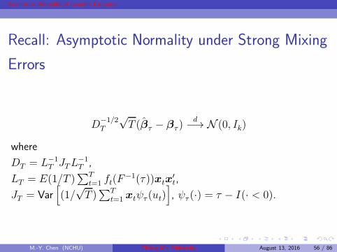
Recall: Asymptotic Normality under Strong Mixing
Errors
D−1/2T
√T (βτ − βτ )
d−→ N (0, Ik)
where
DT = L−1T JTL
−1T ,
LT = E(1/T )∑T
t=1 ft(F−1(τ))xtx
′t,
JT = Var[
(1/√T )∑T
t=1 xtψτ (ut)]
, ψτ (·) = τ − I(· < 0).
M.-Y. Chen (NCHU) Chiang-Mai University August 13, 2016 56 / 86
Page 62
Asymptotic Normality of Quantile Estimator
Testing H0 : Rβτ = r
Wald Test: By Theorem 5.2, we have
R√T (βτ − βτ )
d−→ N (0,RDTR′),
or equivalently
Γ−1/2T R
√T (βτ − βτ )
d−→ N (0, Iq),
where ΓT = RDTR′.
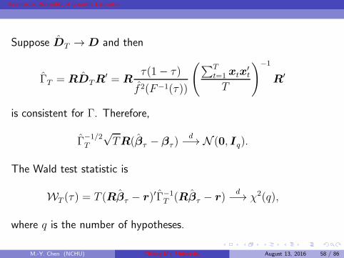
M.-Y. Chen (NCHU) Chiang-Mai University August 13, 2016 57 / 86
Page 63
Asymptotic Normality of Quantile Estimator
Suppose DT → D and then
ΓT = RDTR′ = R
τ(1− τ)
f 2(F−1(τ))
(
∑Tt=1 xtx
′t
T
)−1
R′
is consistent for Γ. Therefore,
Γ−1/2T
√TR(βτ − βτ )
d−→ N (0, Iq).
The Wald test statistic is
WT (τ) = T (Rβτ − r)′Γ−1T (Rβτ − r)
d−→ χ2(q),
where q is the number of hypotheses.
M.-Y. Chen (NCHU) Chiang-Mai University August 13, 2016 58 / 86
Page 64
Asymptotic Normality of Quantile Estimator
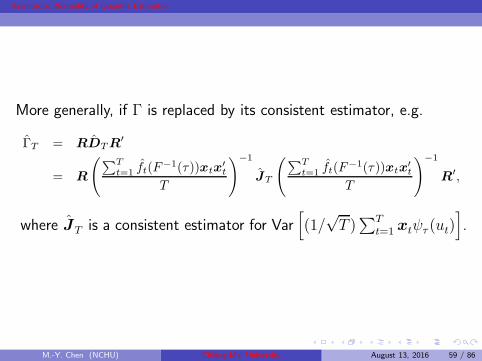
More generally, if Γ is replaced by its consistent estimator, e.g.
ΓT = RDTR′
= R
(
∑Tt=1 ft(F
−1(τ))xtx′t
T
)−1
JT
(
∑Tt=1 ft(F
−1(τ))xtx′t
T
)−1
R′,
where JT is a consistent estimator for Var[
(1/√T )∑T
t=1 xtψτ (ut)]
.
M.-Y. Chen (NCHU) Chiang-Mai University August 13, 2016 59 / 86
Page 65
Asymptotic Normality of Quantile Estimator
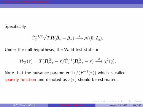
Specifically,
Γ−1/2T
√TR(βτ − βτ )
d−→ N (0, Iq).
Under the null hypothesis, the Wald test statistic
WT (τ) = T (Rβτ − r)′Γ−1T (Rβτ − r)
d−→ χ2(q),
Note that the nuisance parameter 1/f(F−1(τ)) which is called
sparsity function and denoted as s(τ) should be estimated.
M.-Y. Chen (NCHU) Chiang-Mai University August 13, 2016 60 / 86
Page 66
Asymptotic Normality of Quantile Estimator
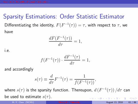
Sparsity Estimations: Order Statistic EstimatorDifferentiating the identity, F (F−1(τ)) = τ , with respect to τ , we
have
dF (F−1(τ))
dτ= 1,
i.e.
f(F−1(τ)) · dF−1(τ)
dτ= 1,
and accordingly
s(τ) ≡ d
dτF−1(τ) =
1
f(F−1(τ)),
where s(τ) is the sparsity function. Thereupon, d (F−1(τ)) /dτ can
be used to estimate s(τ).M.-Y. Chen (NCHU) Chiang-Mai University August 13, 2016 61 / 86
Page 67
Asymptotic Normality of Quantile Estimator
By observing that
d
dτF−1(τ) = lim
h→0
1
2
[
F−1(τ + h)− F−1(τ)
h+F−1(τ)− F−1(τ − h)
h
]
,
it is natural to estimate s(τ) through
sT (τ) =F−1T (τ + hT )− F−1
T (τ − hT )
2hT,
where F−1T (·) is an estimate of F−1(·) and hT is a bandwidth which
tends to zero as T → ∞.
M.-Y. Chen (NCHU) Chiang-Mai University August 13, 2016 62 / 86
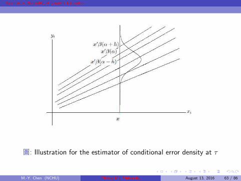
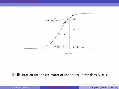
Page 68
Asymptotic Normality of Quantile Estimator
圖: Illustration for the estimator of conditional error density at τ
M.-Y. Chen (NCHU) Chiang-Mai University August 13, 2016 63 / 86
Page 69
Asymptotic Normality of Quantile Estimator
圖: Illustration for the estimator of conditional error density at τ
M.-Y. Chen (NCHU) Chiang-Mai University August 13, 2016 64 / 86
Page 70
Asymptotic Normality of Quantile Estimator
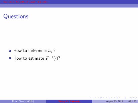
Questions
How to determine hT ?
How to estimate F−1(·)?
M.-Y. Chen (NCHU) Chiang-Mai University August 13, 2016 65 / 86
Page 71
Asymptotic Normality of Quantile Estimator
Bandwidth Selectors
Bofinger Bandwidth Selector:
hT = T−1/5
[
4.5φ4(Φ−1(τ))
(2Φ−1(τ)2 + 1)2
]1/5
,
Hall and Sheather Bandwidth Selector:
hT = T−1/3z2/3α
[
1.5φ2(Φ−1(τ))
2Φ−1(τ)2 + 1
]1/3
.
Chamberlain Bandwidth Selector:
hT = zα√
τ(1− τ)/T .
M.-Y. Chen (NCHU) Chiang-Mai University August 13, 2016 66 / 86
Page 72
Asymptotic Normality of Quantile Estimator
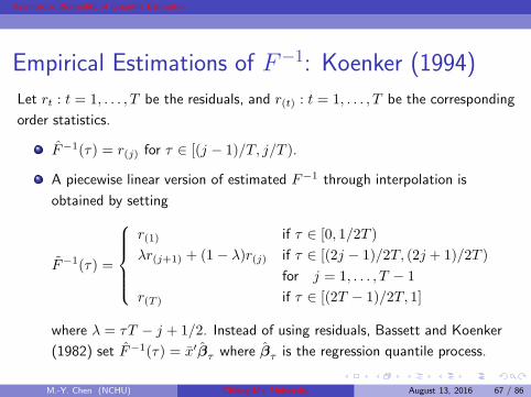
Empirical Estimations of F−1: Koenker (1994)
Let rt : t = 1, . . . , T be the residuals, and r(t) : t = 1, . . . , T be the corresponding
order statistics.
F−1(τ) = r(j) for τ ∈ [(j − 1)/T, j/T ).
A piecewise linear version of estimated F−1 through interpolation is
obtained by setting
F−1(τ) =
r(1) if τ ∈ [0, 1/2T )
λr(j+1) + (1 − λ)r(j) if τ ∈ [(2j − 1)/2T, (2j + 1)/2T )
for j = 1, . . . , T − 1
r(T ) if τ ∈ [(2T − 1)/2T, 1]
where λ = τT − j + 1/2. Instead of using residuals, Bassett and Koenker
(1982) set F−1(τ) = x′βτ where βτ is the regression quantile process.
M.-Y. Chen (NCHU) Chiang-Mai University August 13, 2016 67 / 86
Page 73
Asymptotic Normality of Quantile Estimator
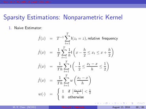
Sparsity Estimations: Nonparametric Kernel
1. Naive Estimator:
f(z) = T−1T∑
t=1
I(zt = z), relative frequency
f(x) =1
T
T∑
t=1
1
hI
(
x− h
2≤ xt ≤ x+
h
2
)
f(x) =1
Th
T∑
t=1
I
(
−1
2≤ xt − x
h≤ 1
2
)
f(x) =1
Th
T∑
t=1
w
(
xt − x
h
)
w(·) =
1 if∣
∣
xt−xh
∣
∣ < 12
0 otherwise
M.-Y. Chen (NCHU) Chiang-Mai University August 13, 2016 68 / 86
Page 74
Asymptotic Normality of Quantile Estimator
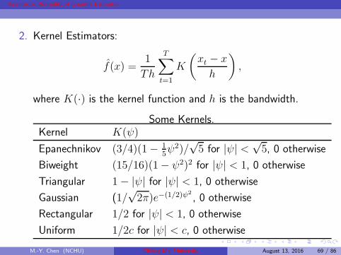
2. Kernel Estimators:
f(x) =1
Th
T∑
t=1
K
(
xt − x
h
)
,
where K(·) is the kernel function and h is the bandwidth.
Some Kernels.Kernel K(ψ)
Epanechnikov (3/4)(1− 15ψ2)/
√5 for |ψ| <
√5, 0 otherwise
Biweight (15/16)(1− ψ2)2 for |ψ| < 1, 0 otherwise
Triangular 1− |ψ| for |ψ| < 1, 0 otherwise
Gaussian (1/√2π)e−(1/2)ψ2
, 0 otherwise
Rectangular 1/2 for |ψ| < 1, 0 otherwise
Uniform 1/2c for |ψ| < c, 0 otherwise
M.-Y. Chen (NCHU) Chiang-Mai University August 13, 2016 69 / 86
Page 75
Asymptotic Normality of Quantile Estimator
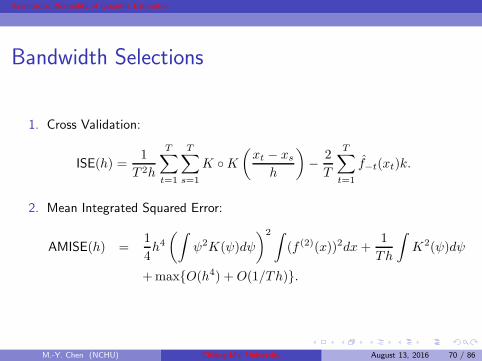
Bandwidth Selections
1. Cross Validation:
ISE(h) =1
T 2h
T∑
t=1
T∑
s=1
K K(
xt − xsh
)
− 2
T
T∑
t=1
f−t(xt)k.
2. Mean Integrated Squared Error:
AMISE(h) =1
4h4(∫
ψ2K(ψ)dψ
)2 ∫
(f (2)(x))2dx +1
Th
∫
K2(ψ)dψ
+maxO(h4) +O(1/Th).
M.-Y. Chen (NCHU) Chiang-Mai University August 13, 2016 70 / 86
Page 76
Asymptotic Normality of Quantile Estimator
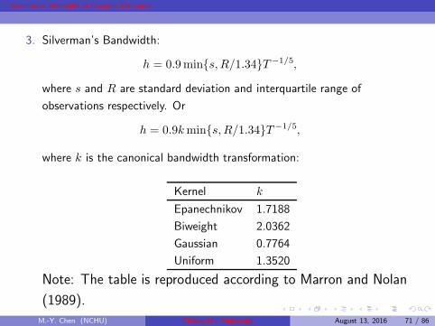
3. Silverman’s Bandwidth:
h = 0.9mins,R/1.34T−1/5,
where s and R are standard deviation and interquartile range of
observations respectively. Or
h = 0.9kmins,R/1.34T−1/5,
where k is the canonical bandwidth transformation:
Kernel k
Epanechnikov 1.7188
Biweight 2.0362
Gaussian 0.7764
Uniform 1.3520
Note: The table is reproduced according to Marron and Nolan
(1989).
M.-Y. Chen (NCHU) Chiang-Mai University August 13, 2016 71 / 86
Page 77
Asymptotic Normality of Quantile Estimator
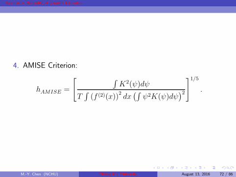
4. AMISE Criterion:
hAMISE =
[
∫
K2(ψ)dψ
T∫
(f (2)(x))2dx(∫
ψ2K(ψ)dψ)2
]1/5
.
M.-Y. Chen (NCHU) Chiang-Mai University August 13, 2016 72 / 86
Page 78
Asymptotic Normality of Quantile Estimator
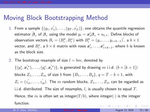
Moving Block Bootstrapping Method
1. From a sample (y1, x′
1), . . . , (yT , x′
T ), one obtains the quantile regression
estimator βτ of βτ using the model yt = x′tβτ + ut,τ . Define blocks of
observation vectors Bi = (Byi , B
xi ) with B
yi = (yi, . . . , yi+b−1)
′
, a b× 1
vector, and Bxi , a b× k matrix with rows x′
i, . . . ,x′i+b−1, where b is known
as the block size.
2. The bootstrap resample of size l = bm, denoted by
(y∗1 ,x′∗1 ), . . . , (y∗l ,x
′∗l ), is generated by drawing m i.i.d. (b × [k + 1])
blocks Z1, . . . , Zm of size b from B1, . . . , Bq, q = T − b + 1, with
Zi = (z′
i1, . . . , z′
ib). The m random blocks, Z1, . . . , Zm can be regarded as
i.i.d. distributed. The size of resamples, l, is usually chosen to equal T .
Hence, the m is often set as integer(T/b), where integer(·) is the integer
function.
M.-Y. Chen (NCHU) Chiang-Mai University August 13, 2016 73 / 86
Page 79
Asymptotic Normality of Quantile Estimator
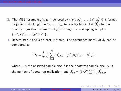
3. The MBB resample of size l, denoted by (y∗1 ,x′∗1 ), . . . , (y∗l ,x
′∗l ) is formed
by joining (stacking) the Z1, . . . , Zm to one big block. Let β∗
τ,l be the
quantile regression estimates of βτ through the resampling samples
(y∗1 ,x′∗1 ), . . . , (y∗l ,x
′∗l ).
4. Repeat step 2 and 3 at least N times. The covariance matrix of βτ can be
computed as
Ωτ =l
T
1
N
N∑
j=1
(β∗
τ,l,j − β∗τ,l)(β
∗
τ,l,j − β∗τ,l)
′,
where T is the observed sample size, l is the bootstrap sample size, N is
the number of bootstrap replication, and β∗τ,l = (1/N)
∑Nj=1 β
∗
τ,l,j.
M.-Y. Chen (NCHU) Chiang-Mai University August 13, 2016 74 / 86
Page 80
Asymptotic Normality of Quantile Estimator
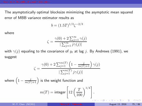
The asymptotically optimal blocksize minimizing the asymptotic mean squared
error of MBB variance estimator results as
b = (1.5T )1/3ζ−2/3
where
ζ =γ(0) + 2
∑∞j=1 γ(j)
|∑∞j=1 jγ(j)|
with γ(j) equaling to the covariance of yt at lag j. By Andrews (1991), we
suggest
ζ =γ(0) + 2
∑m(T )j=1
(
1− jm(T )+1
)
γ(j)
|∑m(T )j=1 jγ(j)|
where(
1− jm(T )+1
)
is the weight function and
m(T ) = integer
[
12
(
T
100
)1/4]
.
M.-Y. Chen (NCHU) Chiang-Mai University August 13, 2016 75 / 86
Page 81
Asymptotic Normality of Quantile Estimator
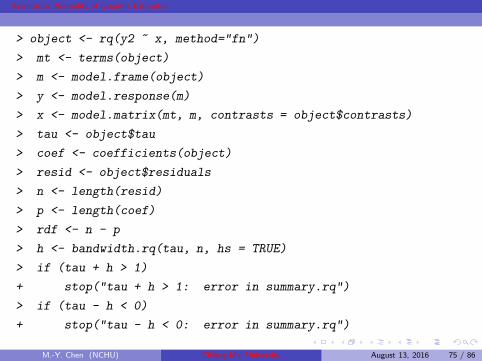
> object <- rq(y2 ~ x, method="fn")
> mt <- terms(object)
> m <- model.frame(object)
> y <- model.response(m)
> x <- model.matrix(mt, m, contrasts = object$contrasts)
> tau <- object$tau
> coef <- coefficients(object)
> resid <- object$residuals
> n <- length(resid)
> p <- length(coef)
> rdf <- n - p
> h <- bandwidth.rq(tau, n, hs = TRUE)
> if (tau + h > 1)
+ stop("tau + h > 1: error in summary.rq")
> if (tau - h < 0)
+ stop("tau - h < 0: error in summary.rq")
M.-Y. Chen (NCHU) Chiang-Mai University August 13, 2016 75 / 86
Page 82
Asymptotic Normality of Quantile Estimator
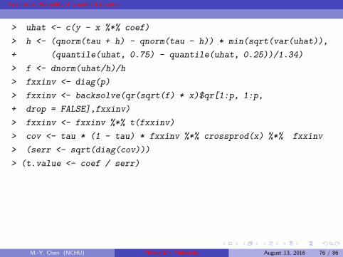
> uhat <- c(y - x %*% coef)
> h <- (qnorm(tau + h) - qnorm(tau - h)) * min(sqrt(var(uhat)),
+ (quantile(uhat, 0.75) - quantile(uhat, 0.25))/1.34)
> f <- dnorm(uhat/h)/h
> fxxinv <- diag(p)
> fxxinv <- backsolve(qr(sqrt(f) * x)$qr[1:p, 1:p,
+ drop = FALSE],fxxinv)
> fxxinv <- fxxinv %*% t(fxxinv)
> cov <- tau * (1 - tau) * fxxinv %*% crossprod(x) %*% fxxinv
> (serr <- sqrt(diag(cov)))
> (t.value <- coef / serr)
M.-Y. Chen (NCHU) Chiang-Mai University August 13, 2016 76 / 86
Page 83
Asymptotic Normality of Quantile Estimator
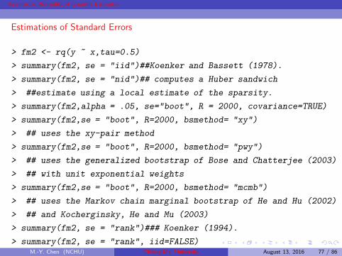
Estimations of Standard Errors
se = ”iid”: presumes that the errors are iid and computes an estimate of the
asymptotic covariance matrix as in KB(1978).
se = ”nid”: presumes local (in tau) linearity (in x) of the the conditional
quantile functions and computes a Huber sandwich estimate using a local
estimate of the sparsity.
se = ”boot”: implements one of several possible bootstrapping alternatives
for estimating standard errors.
se = ”rank”: produces confidence intervals for the estimated parameters by
inverting a rank test as described in Koenker (1994).
se = ”ker”: ”ker”which uses a kernel estimate of the sandwich as proposed
by Powell (1990).
M.-Y. Chen (NCHU) Chiang-Mai University August 13, 2016 76 / 86
Page 84
Asymptotic Normality of Quantile Estimator
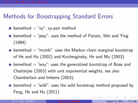
Methods for Boostrapping Standard Errors
bsmethod = ”xy”: xy-pair method
bsmethod = ”pwy”: uses the method of Parzen, Wei and Ying
(1994)
bsmethod = ”mcmb”: uses the Markov chain marginal bootstrap
of He and Hu (2002) and Kocherginsky, He and Mu (2003).
bsmethod = ”wxy”: uses the generalized bootstrap of Bose and
Chatterjee (2003) with unit exponential weights, see also
Chamberlain and Imbens (2003).
bsmethod = ”wild”: uses the wild bootstrap method proposed by
Feng, He and Hu (2011).
M.-Y. Chen (NCHU) Chiang-Mai University August 13, 2016 77 / 86
Page 85
Asymptotic Normality of Quantile Estimator
Estimations of Standard Errors
> fm2 <- rq(y ~ x,tau=0.5)
> summary(fm2, se = "iid")##Koenker and Bassett (1978).
> summary(fm2, se = "nid")## computes a Huber sandwich
> ##estimate using a local estimate of the sparsity.
> summary(fm2,alpha = .05, se="boot", R = 2000, covariance=TRUE)
> summary(fm2,se = "boot", R=2000, bsmethod= "xy")
> ## uses the xy-pair method
> summary(fm2,se = "boot", R=2000, bsmethod= "pwy")
> ## uses the generalized bootstrap of Bose and Chatterjee (2003)
> ## with unit exponential weights
> summary(fm2,se = "boot", R=2000, bsmethod= "mcmb")
> ## uses the Markov chain marginal bootstrap of He and Hu (2002)
> ## and Kocherginsky, He and Mu (2003)
> summary(fm2, se = "rank")### Koenker (1994).
> summary(fm2, se = "rank", iid=FALSE)M.-Y. Chen (NCHU) Chiang-Mai University August 13, 2016 77 / 86
Page 86
Asymptotic Normality of Quantile Estimator
> ## option iid = FALSE implements the proposal of Koenker and
> ## Machado (1999)
M.-Y. Chen (NCHU) Chiang-Mai University August 13, 2016 78 / 86
Page 87
Asymptotic Normality of Quantile Estimator
Provided Tests in quantreg
anova
KhmaladzeTest
M.-Y. Chen (NCHU) Chiang-Mai University August 13, 2016 78 / 86
Page 88
Asymptotic Normality of Quantile Estimator
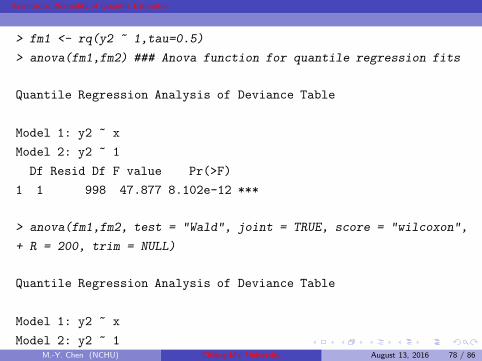
> fm1 <- rq(y2 ~ 1,tau=0.5)
> anova(fm1,fm2) ### Anova function for quantile regression fits
Quantile Regression Analysis of Deviance Table
Model 1: y2 ~ x
Model 2: y2 ~ 1
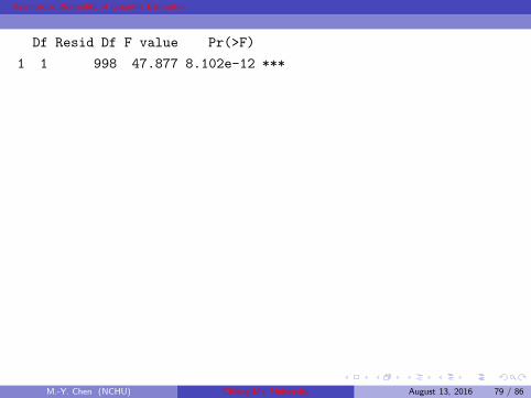
Df Resid Df F value Pr(>F)
1 1 998 47.877 8.102e-12 ***
> anova(fm1,fm2, test = "Wald", joint = TRUE, score = "wilcoxon",
+ R = 200, trim = NULL)
Quantile Regression Analysis of Deviance Table
Model 1: y2 ~ x
Model 2: y2 ~ 1M.-Y. Chen (NCHU) Chiang-Mai University August 13, 2016 78 / 86
Page 89
Asymptotic Normality of Quantile Estimator
Df Resid Df F value Pr(>F)
1 1 998 47.877 8.102e-12 ***
M.-Y. Chen (NCHU) Chiang-Mai University August 13, 2016 79 / 86
Page 90
Asymptotic Normality of Quantile Estimator
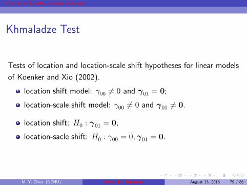
Khmaladze Test
Tests of location and location-scale shift hypotheses for linear models
of Koenker and Xio (2002).
location shift model: γ00 6= 0 and γ01 = 0;
location-scale shift model: γ00 6= 0 and γ01 6= 0.
location shift: H0 : γ01 = 0,
location-sacle shift: H0 : γ00 = 0,γ01 = 0.
M.-Y. Chen (NCHU) Chiang-Mai University August 13, 2016 79 / 86
Page 91
Asymptotic Normality of Quantile Estimator
> KhmaladzeTest(y2 ~ x, data = NULL, taus = -1, nullH = "location")
> KhmaladzeTest(y2 ~ x, taus = seq(.05,.95,by = .01))
> KhmaladzeTest(y2 ~ x, data = NULL, taus = -1,
+ nullH = "location-scale")
M.-Y. Chen (NCHU) Chiang-Mai University August 13, 2016 79 / 86
Page 92
Asymptotic Normality of Quantile Estimator
code: Wald.R
> ## clear all existing objects
> rm(list=ls(all=TRUE))
> options(digits = 4)
> library(quantreg) # For quantile regression
> library(qpcR) # for the Hannan Quinn Criterion
> library(sandwich) #for HAC Estimator
> library(car) #for linearHypothesis
> library(lmtest) #for coeftest
> x1 <- rnorm(1000, 1, 1)
> x2 <- runif(1000)
> x3 <- rnorm(1000, 10, 3)
> e <- rnorm(1000)
> y <- 1 + 0.1*x1 - 0.3 * x2 + 0.2 * x3 + sqrt(x3) * e
> x <- cbind(x1, x2, x3)
>M.-Y. Chen (NCHU) Chiang-Mai University August 13, 2016 79 / 86
Page 93
Asymptotic Normality of Quantile Estimator
> J <- 4 ## Number of linear hypothesis in the null under testing
> R1 <- matrix(0:0, 3, 1)
> R2 <- diag(3)
> R <- cbind(R1, R2)##q*k matrix
> r <- matrix(0:0,3,1)## q*1 vector
>
> ##### Least Squares significance Tests
> fm <- lm(y~x)
> summary(fm)
> linearHypothesis(fm,R,r,vcov=NeweyWest(fm))
> ## need library(sandwich) and library(car)
>
> #### Quantile Regression Linear Hypothesis Test at a tau
> #### ANOVA test
> tau <- 0.5
> fit1 <- rq(y~x1 + x2 + x3, tau)
M.-Y. Chen (NCHU) Chiang-Mai University August 13, 2016 79 / 86
Page 94
Asymptotic Normality of Quantile Estimator
> fit2 <- rq(y~x1, tau)
> anova(fit1,fit2, test = "Wald", joint = TRUE,
+ score = "tau", se = "nid", R = 200, trim = NULL)
>
> #### Wald test for a specific tau
> #fit1 <- rq(y~x, tau, method = "fn")
> betahat <-coef(fit1)
> getcov <-summary.rq(fit1, se="nid", covariance=TRUE, hs = FALSE)
> covm <-(getcov$cov)
> Rbetahat <- R %*% betahat
> Wtau <- t(Rbetahat - r) %*% solve(R %*% covm %*% t(R)) %*% (Rbetahat
> print ("---------Output from the Wtau test:---------")
> print("the quantile of interest is:")
> print(tau)
M.-Y. Chen (NCHU) Chiang-Mai University August 13, 2016 80 / 86
Page 95
Asymptotic Normality of Quantile Estimator
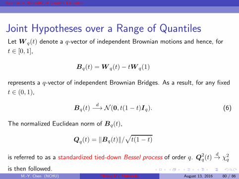
Joint Hypotheses over a Range of QuantilesLet W q(t) denote a q-vector of independent Brownian motions and hence, for
t ∈ [0, 1],
Bq(t) = W q(t)− tW q(1)
represents a q-vector of independent Brownian Bridges. As a result, for any fixed
t ∈ (0, 1),
Bq(t)d−→ N (0, t(1− t)Iq). (6)
The normalized Euclidean norm of Bq(t),
Qq(t) = ‖Bq(t)‖/√
t(1 − t)
is referred to as a standardized tied-down Bessel process of order q. Q2q(t)
d→ χ2q
is then followed.M.-Y. Chen (NCHU) Chiang-Mai University August 13, 2016 80 / 86
Page 96
Asymptotic Normality of Quantile Estimator
And, under the null hypotheses Under the null hypothesis, the Wald
test statistic
maxτ∈T
WT (τ) = maxτ∈T
T (Rβτ − r)′Γ−1T (Rβτ − r)
d−→ supτ∈T
Q2q(τ).
M.-Y. Chen (NCHU) Chiang-Mai University August 13, 2016 81 / 86
Page 97
Asymptotic Normality of Quantile Estimator
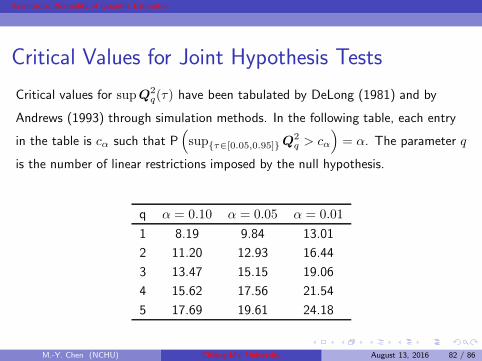
Critical Values for Joint Hypothesis Tests
Critical values for supQ2q(τ) have been tabulated by DeLong (1981) and by
Andrews (1993) through simulation methods. In the following table, each entry
in the table is cα such that P(
supτ∈[0.05,0.95]Q2q > cα
)
= α. The parameter q
is the number of linear restrictions imposed by the null hypothesis.
q α = 0.10 α = 0.05 α = 0.01
1 8.19 9.84 13.01
2 11.20 12.93 16.44
3 13.47 15.15 19.06
4 15.62 17.56 21.54
5 17.69 19.61 24.18
M.-Y. Chen (NCHU) Chiang-Mai University August 13, 2016 82 / 86
Page 98
Asymptotic Normality of Quantile Estimator
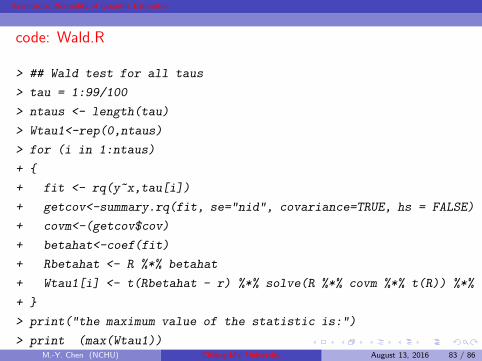
code: Wald.R
> ## Wald test for all taus
> tau = 1:99/100
> ntaus <- length(tau)
> Wtau1<-rep(0,ntaus)
> for (i in 1:ntaus)
+
+ fit <- rq(y~x,tau[i])
+ getcov<-summary.rq(fit, se="nid", covariance=TRUE, hs = FALSE)
+ covm<-(getcov$cov)
+ betahat<-coef(fit)
+ Rbetahat <- R %*% betahat
+ Wtau1[i] <- t(Rbetahat - r) %*% solve(R %*% covm %*% t(R)) %*% (Rbetahat
+
> print("the maximum value of the statistic is:")
> print (max(Wtau1))M.-Y. Chen (NCHU) Chiang-Mai University August 13, 2016 83 / 86
Page 99
Asymptotic Normality of Quantile Estimator
Average Treatment Effect (ATE)
Evaluating the impact of a treatment (program, policy, intervention).
Let D be the binary indicator of treatment and X be covariates.
Y1(Y0) is the potential outcome when an agent is (is not)
exposed to the treatment.
The observed outcome is Y = DY1 + (1−D)Y0.
We observe only one potential outcome (Y1i or Y0i) and hence can not
identify the individual treatment effect, Y1i − Y0i . We may estimate the
ATE: E(Y1 − Y0).
Under conditional independence: (Y1, Y0)⊥D|X ,
E(Y |D = 1, X)− E(Y |D = 0, X) = E(Y1 − Y0|X),
so that the ATE is E(Y1 − Y0) = E[E(Y1 − Y0|X)].
M.-Y. Chen (NCHU) Chiang-Mai University August 13, 2016 83 / 86
Page 100
Asymptotic Normality of Quantile Estimator
Using the sammpe counterpart of
E(Y |D = 1, X)−E(Y |D = 0, X), we have
ATE =1
n
n∑
i=1
[E(Yi|Di = 1, Xi)− E(Yi|Di = 0, Xi)].
For the dummy-variable regression:
Yi = α +Diγ +X ′iβ + ei, i = 1, . . . , n,
the LS estimate of γ is ATE.
Other estimators: Kernel matching, nearest neighbor matching,
propensity score matching (based on p(x) = P (D = 1|X = x)),
etc.
M.-Y. Chen (NCHU) Chiang-Mai University August 13, 2016 84 / 86
Page 101
Asymptotic Normality of Quantile Estimator
Quantile Treatment Effect (QTE)
Let F0 and F1 be the distributions of control and treatment responses. Let
(η) be the“horizontal shift” from F0 to F1: F0(η) = F1(η +(η)).
Then, (η) = F−11 (F0(η))− η, and the τth QTE is, for F0(η) = τ ,
QTE(τ) = F−11 (τ) − F−1
0 (τ) = qY1(τ) − qY0(τ),
the difference between the quantiles of two distributions.
The quantile regression:
Yi = α+Diγ +X ′iβ + ei,
the resulting QR estimate γ(τ) is the estimated τth QTE.
Other: A weighting estimator based on the propensity score.
M.-Y. Chen (NCHU) Chiang-Mai University August 13, 2016 85 / 86
Page 102
Asymptotic Normality of Quantile Estimator
Difference in Differences
To identify the“true” treatment effect, the potential change due to time
(other factors) must be excluded first.
Define the following dummy variables:Di,at = Di,t ×Di,a.
Di,t = 1 if the ith individual receives the treatment;
Di,a = 1 if the ith individual is in the post-program period;
Model: Yi = α+ α1Di,t + α2Di,a + α3Di,at +Xiβ + ei.
For the treatment group in pre- and post-program periods, the
time effect is α2 + α3.
For the control group in pre- and post-program periods, the
time effect is α2.
The treatment effect is the difference between these two effects:
α3.M.-Y. Chen (NCHU) Chiang-Mai University August 13, 2016 86 / 86