Quantitative analysis of Förster resonance energy transfer from spectrally resolved fluorescence measurements PhD Thesis in partial fulfilment of the requirements for the degree “Doctor of Philosophy (PhD)” in the Neuroscience Program at the Georg August University Göttingen, Faculty of Biology submitted by Andrew T. Woehler born in Phoenix, Arizona, USA Goettingen, 2010
Transcript
Quantitative analysis of Förster resonance energy transfer
from spectrally resolved fluorescence measurements
PhD Thesis
in partial fulfilment of the requirements
for the degree “Doctor of Philosophy (PhD)”
in the Neuroscience Program
at the Georg August University Göttingen,
Faculty of Biology
submitted by
Andrew T. Woehler
born in
Phoenix, Arizona, USA
Goettingen, 2010
ii
Supervisor, PhD committee member: Prof. Dr. Erwin Neher
Supervisor, PhD committee member: Prof. Dr. Evgeni Ponimaskin
PhD committee member: Prof. Dr. Dr. Detlev Schild
Date of submission of the PhD thesis: March 17, 2010
iii
I hereby declare that I prepared this PhD thesis, entitled “Quantitative analysis of Förster resonance
energy transfer from spectrally resolved fluorescence measurements”, on my own and with no other
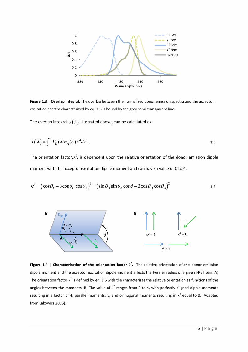
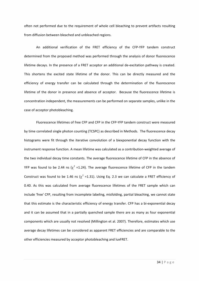
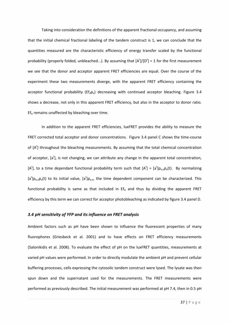
which we have shown not to be affected by YFP bleaching, is not affected by changes in pH as well.
Panel C of figure 3.5 shows that at the low pH extreme the measured EfA becomes unstable,
indicated by inconsistent values at pH 5.5 and unreasonable values at pH 5.0. The total acceptor to
total donor ratio shows a dependency similar to that of EfD. The fitted parameters of the Hill
equation are similar, with pKa = 6.6, n=0.9. Also apparent in this figure, the emission of YFP is almost
completely abolished, as the ratio approaches 0 at pH 4.5.
3.5 Identification of intermolecular interaction
In the case of homo-oligomeric interaction, the apparent fractional occupancies, fD and fA are
dependent on expression ratio of the donor and acceptor. As the donor fraction of a sample is
decreased, the probability of donor-donor complex formation also decreases. In the case of high
affinity interactions (Kd much less than total concentration) it would be expected that all donors
molecules are occupied with acceptors at the lower limit of donor fraction values. In this case it can
be assumed that fd=1 and the apparent FRET efficiency measured estimates Epa. In the case of lower
affinity interaction (i.e. Kd near the total concentration) we would expect a combination of donor
molecules occupied with acceptors as well as free donors but no donor-donor interaction. For this
reason, it is important to measure and take into consideration the relative abundances of donor and
acceptor molecules when comparing apparent FRET efficiencies between samples.
The apparent FRET efficiencies, EfD and EfA, were measured from N1E-115 cells co-expressing
5HT1A-CFP and 5HT1A-YFP. Similar measurements of CD28 and CD86 were used as controls for
discrimination between specific and non-specific interaction. CD28 is an immune-receptor that has
been shown to form covalent dimers in the plasma membrane (Greene et al. 1996; Lazar-Molnar et
al. 2006). CD86, a receptor also found at the immunological synapse, is a monomeric ligand of the
CD28 complex (Sansom et al. 2003; James et al. 2006). Both of these proteins have been used as
positive and negative controls in methods which study protein-protein interaction with fluorescence
and bioluminescence techniques (James et al. 2006; Bouvier et al. 2007; Dorsch et al. 2009).
40 | P a g e
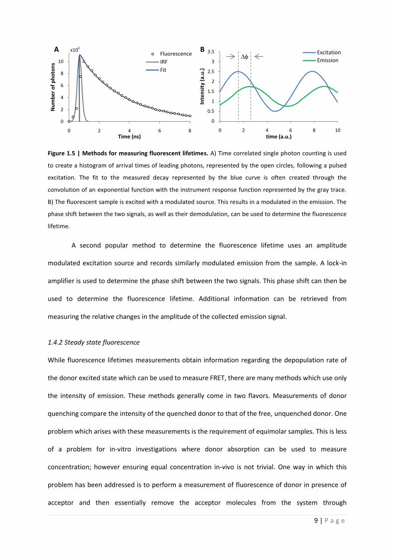
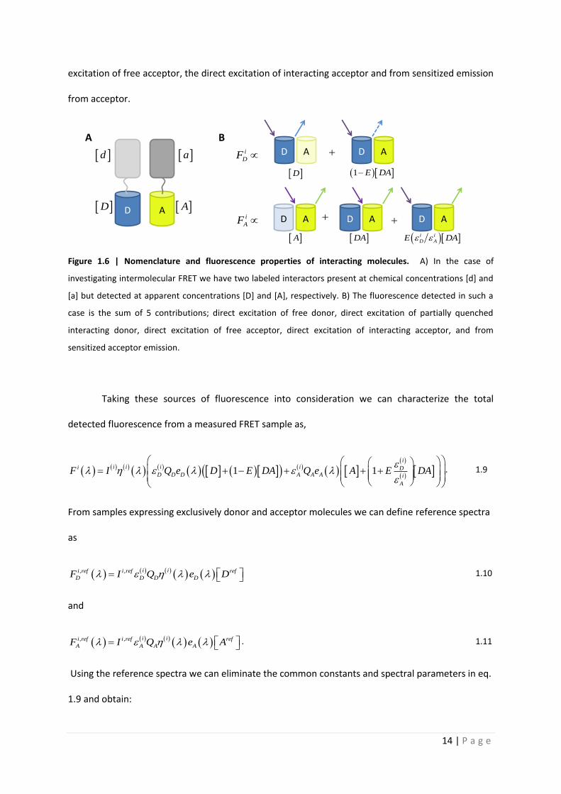
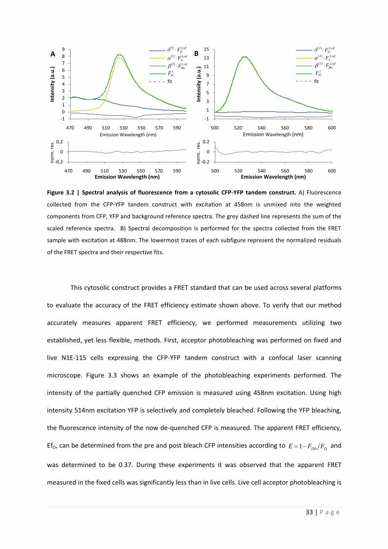
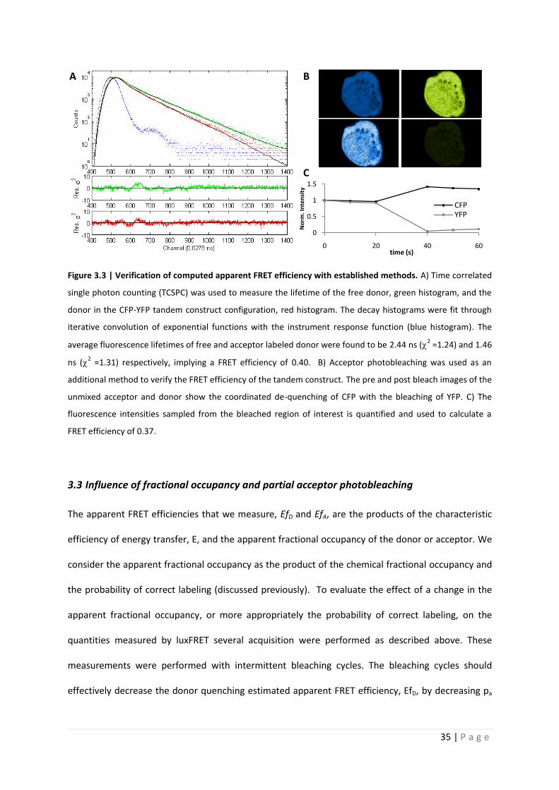
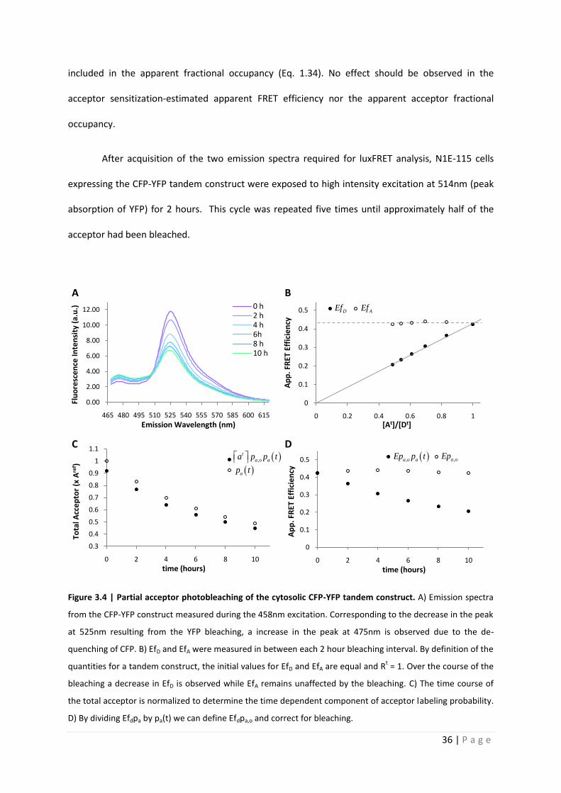
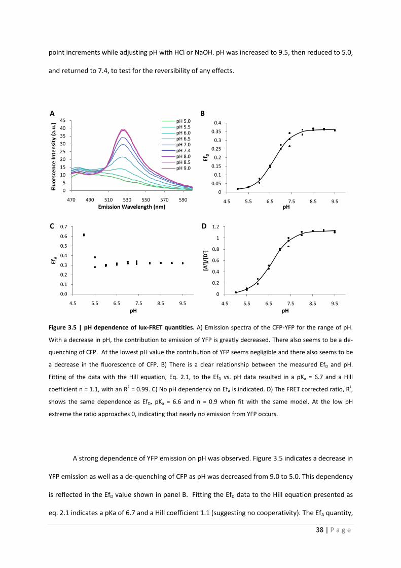
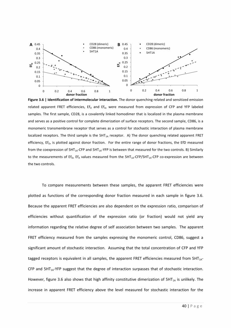
Figure 3.6 | Identification of intermolecular interaction. The donor quenching related and sensitized emission
related apparent FRET efficiencies, EfD and EfA, were measured from expression of CFP and YFP labeled
samples. The first sample, CD28, is a covalently linked homodimer that is localized in the plasma membrane
and serves as a positive control for complete dimerization of surface receptors. The second sample, CD86, is a
monomeric transmembrane receptor that serves as a control for stochastic interaction of plasma membrane
localized receptors. The third sample is the 5HT1A receptor. A) The donor quenching related apparent FRET
efficiency, EfD, is plotted against donor fraction. For the entire range of donor fractions, the EfD measured
from the coexpression of 5HT1A-CFP and 5HT1A-YFP is between that measured for the two controls. B) Similarly
to the measurements of EfD, EfA values measured from the 5HT1A-CFP/5HT1A-CFP co-expression are between
the two controls.
To compare measurements between these samples, the apparent FRET efficiencies were
plotted as functions of the corresponding donor fraction measured in each sample in figure 3.6.
Because the apparent FRET efficiencies are also dependent on the expression ratio, comparison of
efficiencies without quantification of the expression ratio (or fraction) would not yield any
information regarding the relative degree of self association between two samples. The apparent
FRET efficiency measured from the samples expressing the monomeric control, CD86, suggest a
significant amount of stochastic interaction. Assuming that the total concentration of CFP and YFP
tagged receptors is equivalent in all samples, the apparent FRET efficiencies measured from 5HT1A-
CFP and 5HT1A-YFP suggest that the degree of interaction surpasses that of stochastic interaction.
However, figure 3.6 also shows that high affinity constitutive dimerization of 5HT1A is unlikely. The
increase in apparent FRET efficiency above the level measured for stochastic interaction for the
0
0.05
0.1
0.15
0.2
0.25
0.3
0.35
0.4
0.45
0 0.2 0.4 0.6 0.8 1
EfD
donor fraction
CD28 (dimeric)CD86 (monomeric)5HT1A
0
0.05
0.1
0.15
0.2
0.25
0.3
0.35
0.4
0.45
0 0.2 0.4 0.6 0.8 1
EFA
donor fraction
CD28 (dimeric)
CD86 (monomeric)
5HT1A
A B
41 | P a g e
covalently dimerized CD28 is more than double that of the 5HT1A receptor. This could be due to the
adoption of a conformation more favorable to FRET in the case of the CD28 tagged constructs. This
conformation could result in a closer interaction or a more favorable orientation of the fluorescent
proteins. However, assuming that these factors are equal between the CD28 and 5HT1A constructs, it
can be concluded there is some self association between 5HT1A receptors with a substantial portion,
>50%, existing in a monomeric configuration.
3.6 Spectral imaging and implementation of luxFRET to microscopy
The method presented above is one of many methods categorized as spectral FRET methods due to
the requirement of at least two distinct spectral channels from which donor and acceptor emission is
collected. Although two channels are sufficient for the separation of two fluorescent contributions,
when implementing this method to microscopy, the Zeiss LSM510 Meta system was used to
measure fluorescence at a spectral resolution of up to 10.7nm over eight channels simultaneously.
Implementation of luxFRET to spectral microscopy can be performed analogously to its
implementation to spectroscopy, shown above, although at a lower spectral resolution.
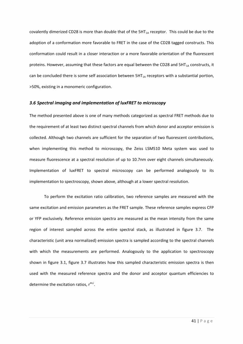
To perform the excitation ratio calibration, two reference samples are measured with the
same excitation and emission parameters as the FRET sample. These reference samples express CFP
or YFP exclusively. Reference emission spectra are measured as the mean intensity from the same
region of interest sampled across the entire spectral stack, as illustrated in figure 3.7. The
characteristic (unit area normalized) emission spectra is sampled according to the spectral channels
with which the measurements are performed. Analogously to the application to spectroscopy
shown in figure 3.1, figure 3.7 illustrates how this sampled characteristic emission spectra is then
used with the measured reference spectra and the donor and acceptor quantum efficiencies to
determine the excitation ratios, rex,i.
42 | P a g e
Figure 3.7 | Excitation ratio calibration from spectral images. A) Spectral image of reference samples
expressing exclusively CFP or YFP are acquired with excitation at 458nm and at 488nm. B) The mean intensities
measured from the same region of interest across the spectral stack are used to construct reference spectra.
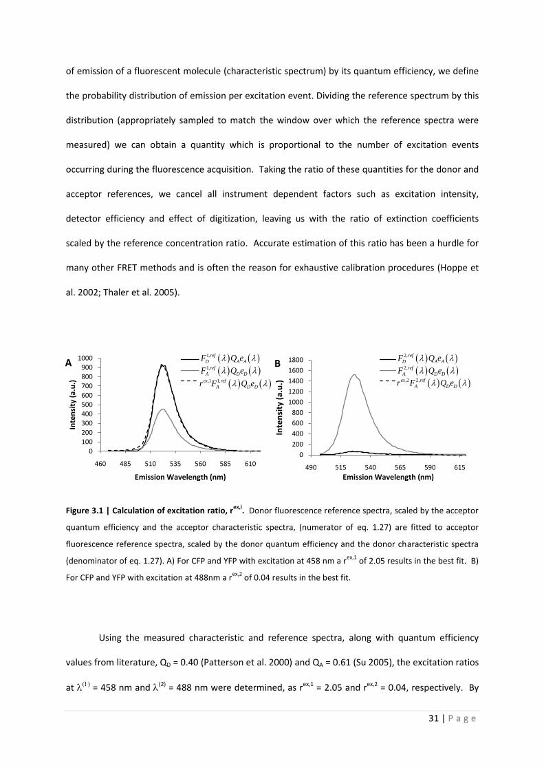
C) Using the measured reference spectra, appropriately sampled characteristic spectra and the donor and
acceptor quantum efficiencies, the excitation ratios, rex,i
can be determined.
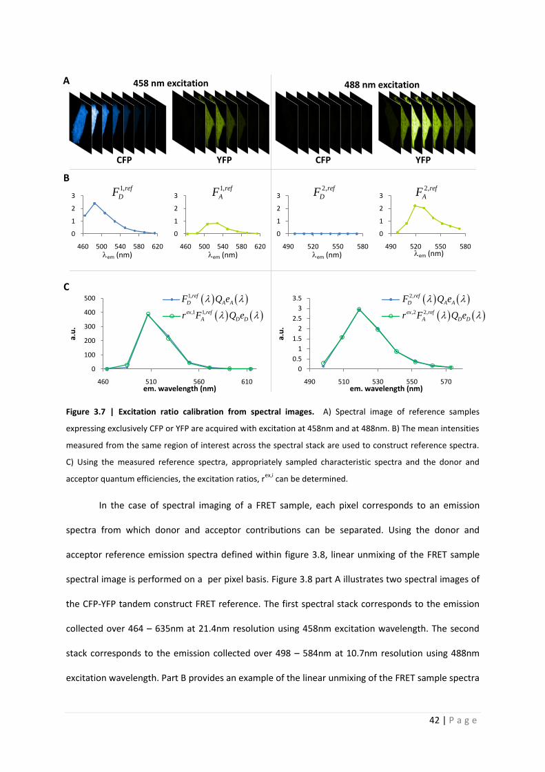
In the case of spectral imaging of a FRET sample, each pixel corresponds to an emission
spectra from which donor and acceptor contributions can be separated. Using the donor and
acceptor reference emission spectra defined within figure 3.8, linear unmixing of the FRET sample
spectral image is performed on a per pixel basis. Figure 3.8 part A illustrates two spectral images of
the CFP-YFP tandem construct FRET reference. The first spectral stack corresponds to the emission
collected over 464 – 635nm at 21.4nm resolution using 458nm excitation wavelength. The second
stack corresponds to the emission collected over 498 – 584nm at 10.7nm resolution using 488nm
excitation wavelength. Part B provides an example of the linear unmixing of the FRET sample spectra
0
1
2
3
460 500 540 580 620
0
1
2
3
460 500 540 580 620
0
1
2
3
490 520 550 580
0
1
2
3
490 520 550 580
0
100
200
300
400
500
460 510 560 610
a.u
.
em. wavelength (nm)
Series1
Series2
0
0.5
1
1.5
2
2.5
3
3.5
490 510 530 550 570
a.u
.
em. wavelength (nm)
Series1
Series2
1,ref
DF 1,ref
AF 2,ref
DF 2,ref
AF
1,ref
D A AF Q e
,1 1,ex ref
A D Dr F Q e
2,ref
D A AF Q e
,2 2,ex ref
A D Dr F Q e
A
B
C
458 nm excitation 488 nm excitation
CFP YFP CFP YFP
em (nm) em (nm) em (nm) em (nm)
43 | P a g e
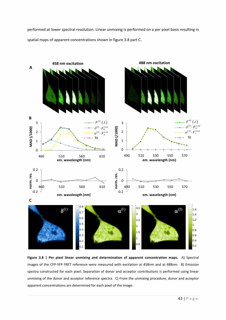
performed at lower spectral resolution. Linear unmixing is performed on a per pixel basis resulting in
spatial maps of apparent concentrations shown in figure 3.8 part C.
Figure 3.8 | Per pixel linear unmixing and determination of apparent concentration maps. A) Spectral
images of the CFP-YFP FRET reference were measured with excitation at 458nm and at 488nm. B) Emission
spectra constructed for each pixel. Separation of donor and acceptor contributions is performed using linear
unmixing of the donor and acceptor reference spectra. C) From the unmixing procedure, donor and acceptor
apparent concentrations are determined for each pixel of the image.
0
1
2
3
460 510 560 610
MA
D (
/10
00
)
em. wavelength (nm)
CFP-YFP
CFP
Series3
fit
0
1
2
3
490 510 530 550 570
MA
D (
/10
00
)
em. wavelength (nm)
Series1
Series2
Series3
Series4
-0.2
0
0.2
460 510 560 610no
rm. r
es.
em. wavelength (nm)-0.2
0
0.2
490 510 530 550 570no
rm. r
es.
em. wavelength (nm)
0.1
0.2
0.3
0.4
0.5
0.6
0.7
0.8
0.5
1
1.5
2
2.5
3
3.5
0.2
0.4
0.6
0.8
1
1.2
1.4
1.6
458 nm excitation 488 nm excitation A
B
C
TCF 1 1,ref
DF 1 1,ref
AF
TCF 2 2,ref
DF 2 2,ref
AF
fit
44 | P a g e
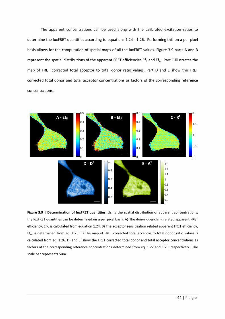
The apparent concentrations can be used along with the calibrated excitation ratios to
determine the luxFRET quantities according to equations 1.24 - 1.26. Performing this on a per pixel
basis allows for the computation of spatial maps of all the luxFRET values. Figure 3.9 parts A and B
represent the spatial distributions of the apparent FRET efficiencies EfD and EfA. Part C illustrates the
map of FRET corrected total acceptor to total donor ratio values. Part D and E show the FRET
corrected total donor and total acceptor concentrations as factors of the corresponding reference
concentrations.
Figure 3.9 | Determination of luxFRET quantities. Using the spatial distribution of apparent concentrations,
the luxFRET quantities can be determined on a per pixel basis. A) The donor quenching related apparent FRET
efficiency, EfD, is calculated from equation 1.24. B) The acceptor sensitization related apparent FRET efficiency,
EfA, is determined from eq. 1.25. C) The map of FRET corrected total acceptor to total donor ratio values is
calculated from eq. 1.26. D) and E) show the FRET corrected total donor and total acceptor concentrations as
factors of the corresponding reference concentrations determined from eq. 1.22 and 1.23, respectively. The
scale bar represents 5um.
0
0.1
0.2
0.3
0.4
0.5
0
0.1
0.2
0.3
0.4
0.5
0
0.5
1
1.5
2
0.2
0.4
0.6
0.8
1
0.2
0.4
0.6
0.8
1
1.2
1.4
1.6
A - EfD B - EfA C - Rt
D - Dt E - At
45 | P a g e
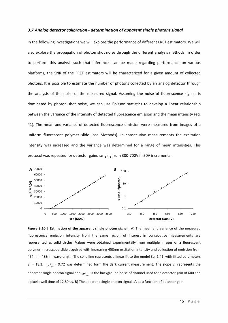
3.7 Analog detector calibration - determination of apparent single photons signal
In the following investigations we will explore the performance of different FRET estimators. We will
also explore the propagation of photon shot noise through the different analysis methods. In order
to perform this analysis such that inferences can be made regarding performance on various
platforms, the SNR of the FRET estimators will be characterized for a given amount of collected
photons. It is possible to estimate the number of photons collected by an analog detector through
the analysis of the noise of the measured signal. Assuming the noise of fluorescence signals is
dominated by photon shot noise, we can use Poisson statistics to develop a linear relationship
between the variance of the intensity of detected fluorescence emission and the mean intensity (eq.
41). The mean and variance of detected fluorescence emission were measured from images of a
uniform fluorescent polymer slide (see Methods). In consecutive measurements the excitation
intensity was increased and the variance was determined for a range of mean intensities. This
protocol was repeated for detector gains ranging from 300-700V in 50V increments.
Figure 3.10 | Estimation of the apparent single photon signal. A) The mean and variance of the measured
fluorescence emission intensity from the same region of interest in consecutive measurements are
represented as solid circles. Values were obtained experimentally from multiple images of a fluorescent
polymer microscope slide acquired with increasing 458nm excitation intensity and collection of emission from
464nm - 485nm wavelength. The solid line represents a linear fit to the model Eq. 1.41, with fitted parameters
's = 18.3. 2
,o i = 9.72 was determined form the dark current measurement. The slope 's represents the
apparent single photon signal and 2
,o i is the background noise of channel used for a detector gain of 600 and
a pixel dwell time of 12.80 us. B) The apparent single photon signal, s’, as a function of detector gain.
0
10000
20000
30000
40000
50000
60000
70000
0 500 1000 1500 2000 2500 3000 3500
F
(MA
D2 )
<F> (MAD)
0.1
1
10
100
250 350 450 550 650 750
s' (
MA
D/p
ho
ton
)
Detector Gain (V)
A B
46 | P a g e
Figure 3.10 shows the best fit of eq. 1.41 to the measured variance of fluorescence
intensities between 300 and 3500 Microscope AD-units (denoted as MADs below) for a detector gain
of 600V. The slope of the linear fit to this data provides a value for the apparent single photon signal,
's = 18.28 MADs/photon. The first point, at the lowest intensity, was performed without excitation.
It is a measurement of the dark current with its x-value representing the detector offset, 286 MADs,
and the y-value represents the background detector noise, 2
,o i = 9.72 MAD2. Panel B of this figure
shows s’ as a function of detector gain.
Table 3.1| Emission channel properties.
Channel (nm) Offset (MADs) 2
o (MADs2) s' (MADs/photon)
464 - 485 296.04 9.66 18.29
486 - 507 300.57 11.57 19.56
508 - 528 293.66 10.51 19.27
529 - 550 300.10 9.92 19.31
551 - 571 296.37 8.94 16.10
572 - 592 291.78 8.79 15.80
593 - 614 297.24 7.74 17.68
615 - 636 290.21 10.65 20.26
Mean 295.75 9.72 18.28
The offset and background variance were determined from measurements of dark current (no excitation). The
apparent single photon signal was determined from the mean – variance relationship of measurements of the
uniform fluorescent polymer slide.
Similar results were obtained from measurements performed on N1E-115 cells expressing
the CFP-YFP tandem construct. In these measurements an apparent single photon signal was
determined for each emission channel used in the single excitation wavelength FRET measurements.
Although photophysics would predict s’ to be inversely proportional to wavelength (Neher and
Neher 2004), 's and 2
,o i were found to be relatively wavelength invariant as shown in table 3.1.
For the luxFRET measurements presented later, the detector gain was typically set to 550 or 600V,
47 | P a g e
resulting in an apparent single photon signal of 9.2 or 18.3 MADs per photon, allowing for the
detection of a maximum of approximately 225 or 500 photons per channel per 12-bit acquisition,
respectively.
It was observed during preliminary measurements that there was a dependency of the
apparent single photon signal on pixel dwell time (scan speed) used during the image acquisition.
Generally higher apparent single photons signals were measured at faster scan speeds. It is assumed
that the manufacture intended for this relationship so that the user could increase the SNR of a
measurement by changing the pixel dwell time, collect more photons, without reconfiguring the
detector gain and/or excitation intensity. It is not clear how this processing is handled however we
have no evidence that it affects our analysis.
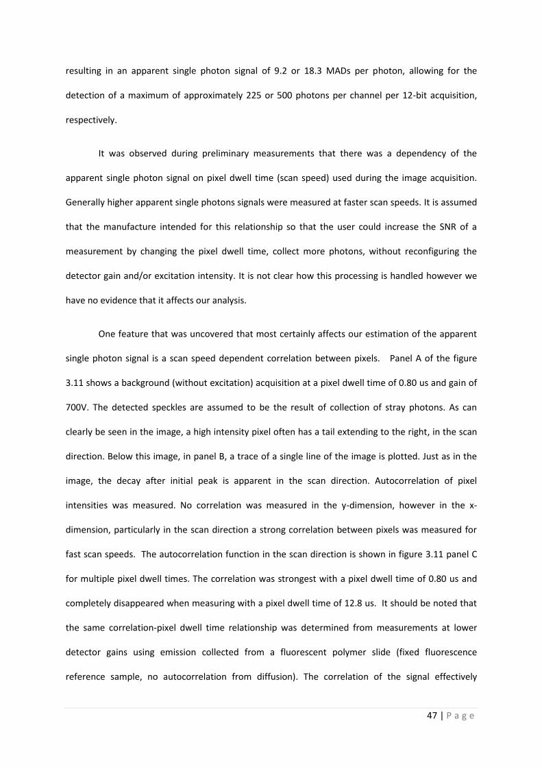
One feature that was uncovered that most certainly affects our estimation of the apparent
single photon signal is a scan speed dependent correlation between pixels. Panel A of the figure
3.11 shows a background (without excitation) acquisition at a pixel dwell time of 0.80 us and gain of
700V. The detected speckles are assumed to be the result of collection of stray photons. As can
clearly be seen in the image, a high intensity pixel often has a tail extending to the right, in the scan
direction. Below this image, in panel B, a trace of a single line of the image is plotted. Just as in the
image, the decay after initial peak is apparent in the scan direction. Autocorrelation of pixel
intensities was measured. No correlation was measured in the y-dimension, however in the x-
dimension, particularly in the scan direction a strong correlation between pixels was measured for
fast scan speeds. The autocorrelation function in the scan direction is shown in figure 3.11 panel C
for multiple pixel dwell times. The correlation was strongest with a pixel dwell time of 0.80 us and
completely disappeared when measuring with a pixel dwell time of 12.8 us. It should be noted that
the same correlation-pixel dwell time relationship was determined from measurements at lower
detector gains using emission collected from a fluorescent polymer slide (fixed fluorescence
reference sample, no autocorrelation from diffusion). The correlation of the signal effectively
48 | P a g e
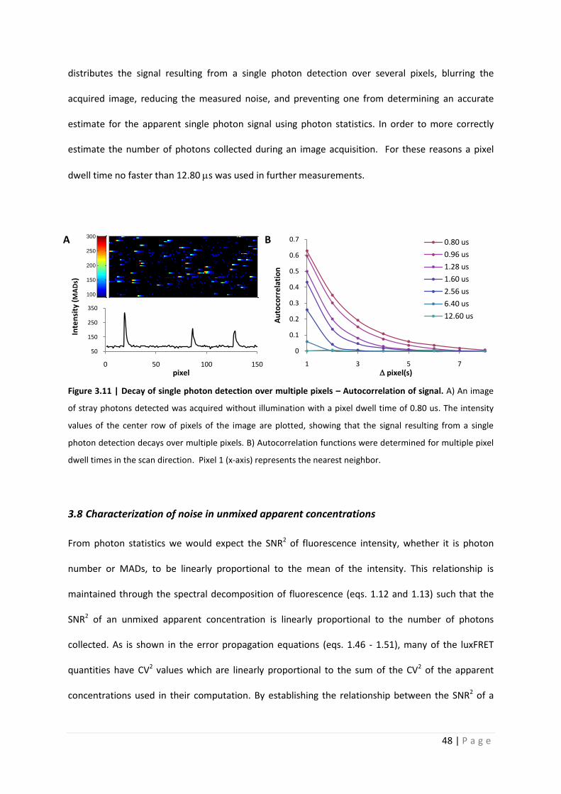
distributes the signal resulting from a single photon detection over several pixels, blurring the
acquired image, reducing the measured noise, and preventing one from determining an accurate
estimate for the apparent single photon signal using photon statistics. In order to more correctly
estimate the number of photons collected during an image acquisition. For these reasons a pixel
dwell time no faster than 12.80 s was used in further measurements.
Figure 3.11 | Decay of single photon detection over multiple pixels – Autocorrelation of signal. A) An image
of stray photons detected was acquired without illumination with a pixel dwell time of 0.80 us. The intensity
values of the center row of pixels of the image are plotted, showing that the signal resulting from a single
photon detection decays over multiple pixels. B) Autocorrelation functions were determined for multiple pixel
dwell times in the scan direction. Pixel 1 (x-axis) represents the nearest neighbor.
3.8 Characterization of noise in unmixed apparent concentrations
From photon statistics we would expect the SNR2 of fluorescence intensity, whether it is photon
number or MADs, to be linearly proportional to the mean of the intensity. This relationship is
maintained through the spectral decomposition of fluorescence (eqs. 1.12 and 1.13) such that the
SNR2 of an unmixed apparent concentration is linearly proportional to the number of photons
collected. As is shown in the error propagation equations (eqs. 1.46 - 1.51), many of the luxFRET
quantities have CV2 values which are linearly proportional to the sum of the CV2 of the apparent
concentrations used in their computation. By establishing the relationship between the SNR2 of a
50
150
250
350
0 50 100 150
Inte
nsi
ty (
MA
Ds)
pixel
0
0.1
0.2
0.3
0.4
0.5
0.6
0.7
1 3 5 7
Au
toco
rre
lati
on
pixel(s)
0.80 us
0.96 us
1.28 us
1.60 us
2.56 us
6.40 us
12.60 us
100
150
200
250
300A B
49 | P a g e
given apparent concentration and the number of photons at which it was detected, we should be
able to make predictions about the SNR2 of the luxFRET quantities at varied photon collection levels.
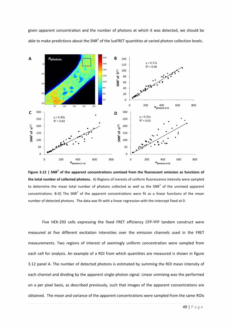
Figure 3.12 | SNR2 of the apparent concentrations unmixed from the fluorescent emission as functions of
the total number of collected photons. A) Regions of inerests of uniform fluorescence intensity were sampled
to determine the mean total number of photons collected as well as the SNR2 of the unmixed apparent
concentrations. B-D) The SNR2 of the apparent concentrations were fit as a linear functions of the mean
number of detected photons. The data was fit with a linear regression with the intercept fixed at 0.
Five HEK-293 cells expressing the fixed FRET efficiency CFP-YFP tandem construct were
measured at five different excitation intensities over the emission channels used in the FRET
measurements. Two regions of interest of seemingly uniform concentration were sampled from
each cell for analysis. An example of a ROI from which quantities are measured is shown in figure
3.12 panel A. The number of detected photons is estimated by summing the ROI mean intensity of
each channel and dividing by the apparent single photon signal. Linear unmixing was the performed
on a per pixel basis, as described previously, such that images of the apparent concentrations are
obtained. The mean and variance of the apparent concentrations were sampled from the same ROIs
50 100 150 200 250
50
100
150
200
250
400
600
800
1000
1200
1400
1600
1800
y = 0.17xR² = 0.96
0
20
40
60
80
100
120
140
0 200 400 600 800
SNR
2o
f
nphotons (i=1)
y = 0.30xR² = 0.83
0
50
100
150
200
250
300
0 200 400 600 800
SNR
2o
f
nphotons (i =1)
y = 0.32xR² = 0.63
0
50
100
150
200
250
300
0 200 400 600 800
SNR
2o
f
nphotons (i=2)
C
B A
D
nphotons
50 | P a g e
as the raw fluorescence signal. The resulting SNR2 of the apparent concentrations were then plotted
against the estimated number of photons collected in figure 3.12 panels B-D. The data were then fit
with a linear regression with the intercept fixed at the origin. The relationships indicated by these
regressions (in figure 3.12) were inverted to characterize the CV2 of the apparent concentrations,
such that they could be used directly in the error propagation equations.
12 1
,15.88 pCV n
, 1
2 1
,13.33 pCV n
, 2
2 1
,23.13 pCV n
. 3.1, 3.2, 3.3
The variances of the unmixed apparent concentrations can also be predicted from a single
set of reference spectra and a single sample spectrum according to eqs. 1.43 – 1.45 (Neher and
Neher 2004). The mean ROI intensity of each channel of the samples used above were used to make
a sample spectrum. Together with the same reference spectra, these sample spectra were used to
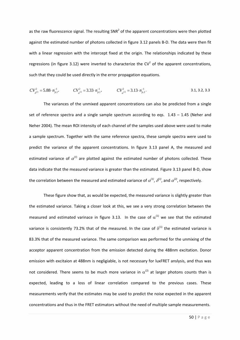
predict the variance of the apparent concentrations. In figure 3.13 panel A, the measured and
estimated variance of (1) are plotted against the estimated number of photons collected. These
data indicate that the measured variance is greater than the estimated. Figure 3.13 panel B-D, show
the correlation between the measured and estimated variance of (1), (1), and (2), respectively.
These figure show that, as would be expected, the measured variance is slightly greater than
the estimated variance. Taking a closer look at this, we see a very strong correlation between the
measured and estimated varinace in figure 3.13. In the case of (1) we see that the estimated
variance is consistently 73.2% that of the measured. In the case of (1) the estimated variance is
83.3% that of the measured variance. The same comparison was performed for the unmixing of the
acceptor apparent concentration from the emission detected during the 488nm excitation. Donor
emission with excitaion at 488nm is negligiable, is not necessary for luxFRET anslysis, and thus was
not considered. There seems to be much more variance in (2) at larger photons counts than is
expected, leading to a loss of linear correlation compared to the previous cases. These
measurements verify that the estimates may be used to predict the noise expected in the apparent
concentrations and thus in the FRET estimators without the need of multiple sample measurements.
51 | P a g e
Figure 3.13 | Measured and estimated variance of the unmixed apparent concentrations. Panel A illustrates
the measured and esimated variance of (1)
as a function of the total number of photons collected. Panel B
indicates the strong correlation of these two variances (a squared coefficent equal to 0.98). Panel C indicates
the strong correlation between the measured and estimated variance of (1)
(a squared coefficent equal to
0.995). Panel D shows the correlation of the estimated and measured variance of (2)
, with a squared
correlation coefficent, R 2, equal to 0.89.
3.9 Use of error propagation to predict SNR2 of FRET estimators.
3.9.1 FRET imaging of an Epac-based cAMP sensor
Two confocal images of N1E-115 cells expressing a Cerulean-Epac-Citrine FRET sensor were acquired
with 458nm and 488nm excitation, respectively, each over 8 emission channels. These images were
first brought into register. Then the apparent concentrations of cerulean, the donor, and citrine, the
acceptor, at each pixel were determined by non-negatively constrained linear unmixing using
previously determined reference spectra. With these apparent concentrations, as well as some
0.00
0.01
0.02
0.03
0.04
0.05
0.06
0.07
0.08
0 200 400 600 800
Var
ian
ce o
f
nphotons (i=1)
MeasuredEstimated
y = 0.7323xR² = 0.9822
0.00
0.01
0.02
0.03
0.04
0.05
0.06
0.00 0.02 0.04 0.06 0.08
Esti
mat
ed
var
. of
(1)
Measured var. of (1)
y = 0.8334xR² = 0.995
0.000
0.001
0.002
0.003
0.004
0.005
0.000 0.001 0.002 0.003 0.004 0.005 0.006
Esti
mat
ed
var
. of
(1)
Measured var. in (1)
y = 0.4334xR² = 0.8896
0.000
0.001
0.002
0.003
0.004
0.005
0.006
0.007
0.000 0.005 0.010 0.015 0.020
Esti
mat
ed
var
. of
(2)
Measured var. in (2)
C D
A B
52 | P a g e
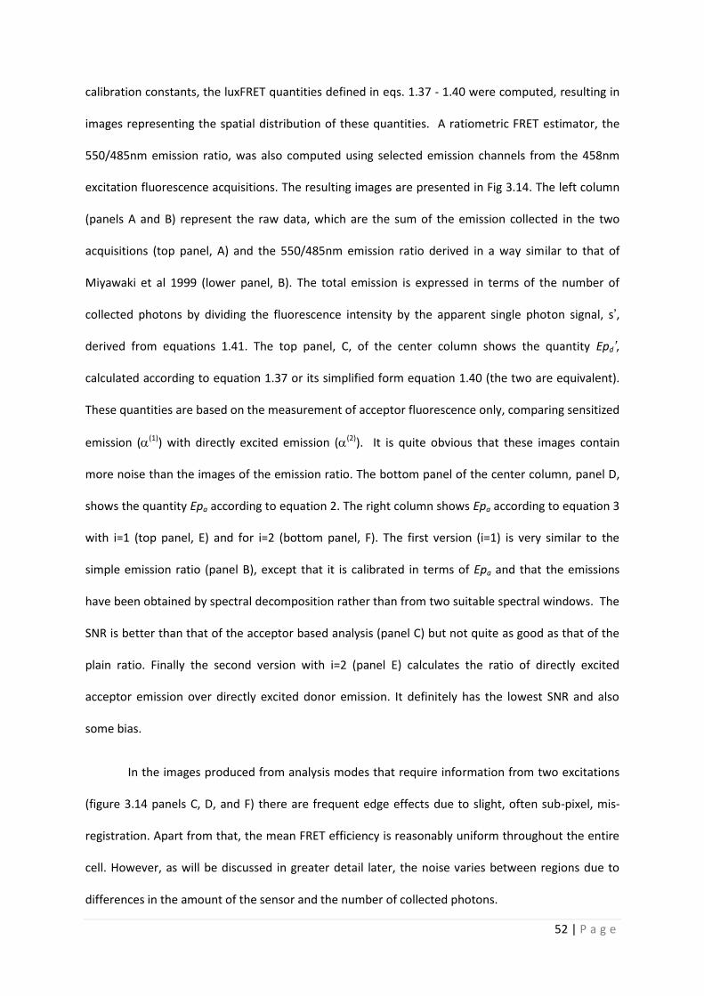
calibration constants, the luxFRET quantities defined in eqs. 1.37 - 1.40 were computed, resulting in
images representing the spatial distribution of these quantities. A ratiometric FRET estimator, the
550/485nm emission ratio, was also computed using selected emission channels from the 458nm
excitation fluorescence acquisitions. The resulting images are presented in Fig 3.14. The left column
(panels A and B) represent the raw data, which are the sum of the emission collected in the two
acquisitions (top panel, A) and the 550/485nm emission ratio derived in a way similar to that of
Miyawaki et al 1999 (lower panel, B). The total emission is expressed in terms of the number of
collected photons by dividing the fluorescence intensity by the apparent single photon signal, s’,
derived from equations 1.41. The top panel, C, of the center column shows the quantity Epd’,
calculated according to equation 1.37 or its simplified form equation 1.40 (the two are equivalent).
These quantities are based on the measurement of acceptor fluorescence only, comparing sensitized
emission ((1)) with directly excited emission ((2)). It is quite obvious that these images contain
more noise than the images of the emission ratio. The bottom panel of the center column, panel D,
shows the quantity Epa according to equation 2. The right column shows Epa according to equation 3
with i=1 (top panel, E) and for i=2 (bottom panel, F). The first version (i=1) is very similar to the
simple emission ratio (panel B), except that it is calibrated in terms of Epa and that the emissions
have been obtained by spectral decomposition rather than from two suitable spectral windows. The
SNR is better than that of the acceptor based analysis (panel C) but not quite as good as that of the
plain ratio. Finally the second version with i=2 (panel E) calculates the ratio of directly excited
acceptor emission over directly excited donor emission. It definitely has the lowest SNR and also
some bias.
In the images produced from analysis modes that require information from two excitations
(figure 3.14 panels C, D, and F) there are frequent edge effects due to slight, often sub-pixel, mis-
registration. Apart from that, the mean FRET efficiency is reasonably uniform throughout the entire
cell. However, as will be discussed in greater detail later, the noise varies between regions due to
differences in the amount of the sensor and the number of collected photons.
53 | P a g e
Figure 3.14 | Comparison of images analysis methods. Confocal images of N1E-115 cells expressing an EPAC
based cytosolic cAMP FRET sensor were analyzed with the various luxFRET and ratiometric methods. A) The
apparent single photon signal was used to estimate the number of photons detected during a sequence of 2
excitations. This number detected within the ROI, shown as a black box, was found to be 3,736 photons per
pixel. B) The YFP to CFP emission ratio was estimated as the ratio of emission in the 550±21nm and 485±21nm
spectral windows. C) Using information from two image acquisitions, with excitation wavelengths 458nm and
488nm, Epd’ was calculated using equation 1.37 or equation 1.40, the two are equivalent. D) Epa was
calculated from dual excitation measurements according to equation 1.38. E) Epa was calculated from a single
acquisition using equation 1.39 with i = 1, and Rt as a calibration constant. F) Epa was also calculated from the
two-excitation wavelength measurement using equation 1.39 with i = 2. To allow for comparison of the
luxFRET quantities to the ratiometric measurement the color scales were adjusted appropriately. Scale bars
represent 5m.
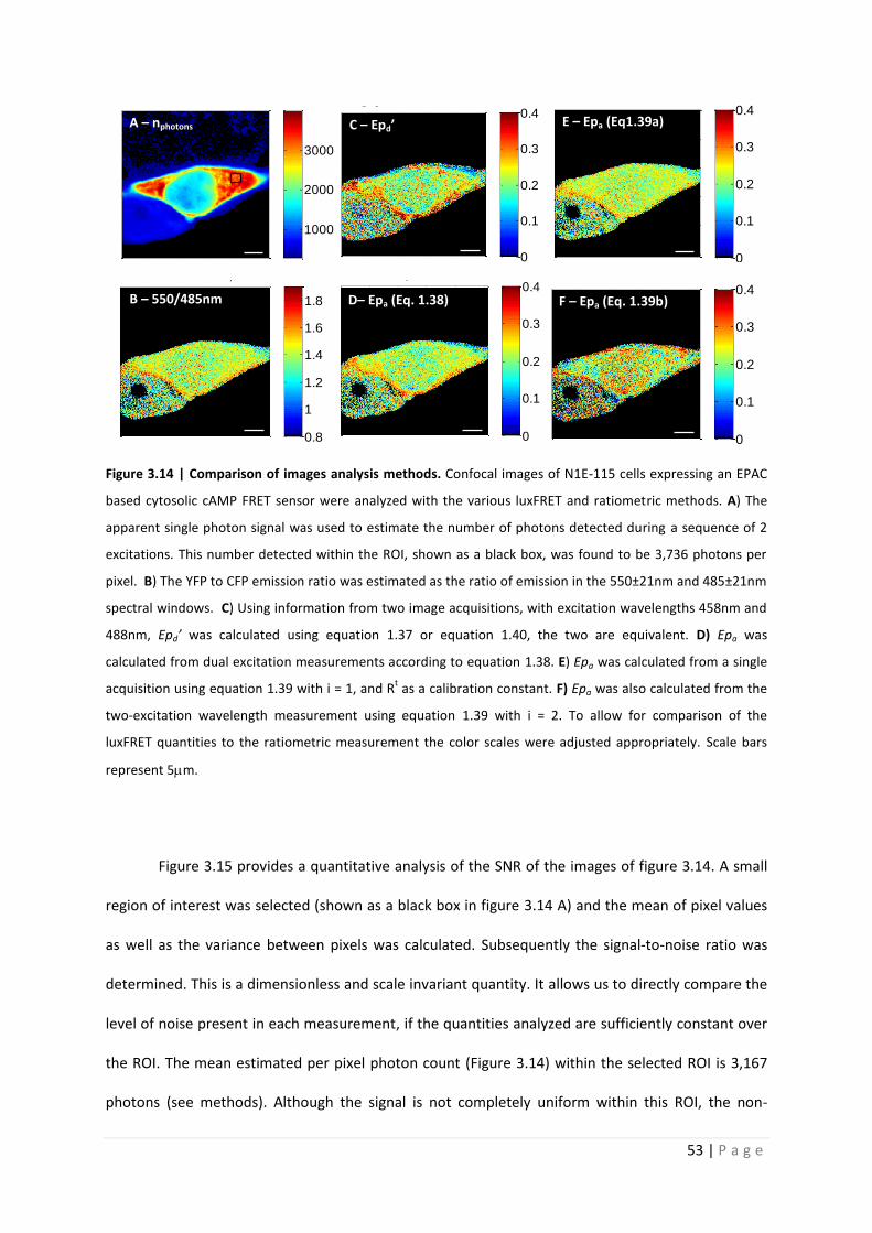
Figure 3.15 provides a quantitative analysis of the SNR of the images of figure 3.14. A small
region of interest was selected (shown as a black box in figure 3.14 A) and the mean of pixel values
as well as the variance between pixels was calculated. Subsequently the signal-to-noise ratio was
determined. This is a dimensionless and scale invariant quantity. It allows us to directly compare the
level of noise present in each measurement, if the quantities analyzed are sufficiently constant over
the ROI. The mean estimated per pixel photon count (Figure 3.14) within the selected ROI is 3,167
photons (see methods). Although the signal is not completely uniform within this ROI, the non-
F1 (mean est. photons =3.17e+003)
1000
2000
3000
Eq. 1, Epd(t
o) = 0.229, SNR
2 = 21.96
0
0.1
0.2
0.3
0.4
Eq. 2 - 1, Ep
a(t
o) = 0.225, SNR
2 = 63.19
0
0.1
0.2
0.3
0.4
Ratio 550nm/485nm = 1.42, SNR2 = 252.6
0.8
1
1.2
1.4
1.6
1.8
EfD = 0.225, SNR2 = 43.92
0
0.1
0.2
0.3
0.4
Eq. 2 - 2, Ep
a(t
o) = 0.22, SNR
2 = 13.82
0
0.1
0.2
0.3
0.4
A – nphotons
B – 550/485nm F – Epa (Eq. 1.39b) D– Epa (Eq. 1.38)
E – Epa (Eq1.39a) C – Epd’
54 | P a g e
uniform concentration should not affect the variance measurement for the derived quantities since
they involve only ratios of two quantities, each of which scales with signal strength. The SNR values
sampled from the quantities illustrated in figure 3.14 are compared in Figure 3.15. This shows, as
was concluded from figure 3.14, that eq. 1.39 (i=1) provides the best SNR of the luxFRET quantities
and that the 550/485nm emission ratio provides the overall best SNR in this example. Differences
between the different analysis modes will be discussed in greater detail later.
Figure 3.15 | Comparison of the FRET indicators. The SNR measured from corresponding ROIs of the
quantities imaged in Figure 3.14 are shown in this bar graph. The results indicate that the 550/485 nm ratio
provides a more favorable SNR than any of the luxFRET quantities. The luxFRET quantity with the most
favorable SNR is Epa calculated with Eq. 1.39 (i=1).
3.9.2 Dependence of SNR2 of FRET estimators on the number of detected photons & FRET efficiency.
To develop the relationship between the SNR2 of our luxFRET quantities and the excitation
intensities, we performed multiple measurement of a CFP-YFP tandem construct at varied excitation
intensities. The measured SNR2 of the apparent concentrations, 1 ,
2 , and
1 , were fit as
linear functions of the estimated number of detected photons (see figure 3.12). These values were
compared to those determined with eqs. 1.43-1.45 and were found to be in good agreement in
figure 3.13.
0
4
8
12
16
20
SNR
55 | P a g e
A thought-experiment was then performed, in which the values for 1 and
i were taken
from the measurement shown in Figure 3.14 (with an Epa of 0.23, n1 = 1,456 photons collected in
458nm excitation acquisition and n2 = 1,711 photons collected during the 488nm excitation
acquisition) and calculated the SNR2-values according to equation 1.48. We simulated changes in
excitation intensity by varying proportionally the number of photons collected. In these calculations
the 1 and
1 values were assumed to be constant (since they are normalized for intensity
changes) and their CV2-values to vary according to the above mentioned linear fitting.
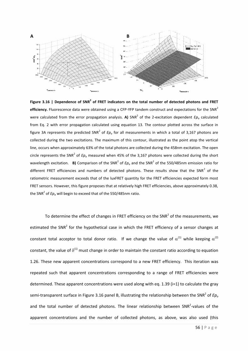
The results of these calculations are shown in figure 3.16 panel A. As would be expected, the
SNR2 of Epa increases with the number of detected photons for both excitations. Interestingly, this
figure suggests that the number photons collected during the respective excitations do not
contribute equally to the SNR of Epa. The contour plotted across the surface in figure 3.16 panel A
represents the predicted SNR2 of Epa for all measurements in which a total of 3,167 photons are
collected during the two excitations. The maximum of this contour, illustrated as the point atop the
solid vertical line, occurs when approximately 63% of the total photons are collected during the
458nm excitation. The open circle, together with the dotted vertical line, represents the measured
SNR2 of Epa sampled from figure 3.14 panel D. In that experiment only 46% of total photons were
collected during the short wavelength. This figure suggests that the SNR2 of Epa could have been
improved by approximately 12% by increasing excitation 1 at the expense of excitation 2. There is a
second reason why it may be advantageous to use lower intensity in the long wavelength excitation,
particularly at high FRET efficiencies. This relates to the fact that the acceptor is subject to bleaching
during both excitations and, therefore, its bleaching may be limiting. This point will be addressed in
more detail in the discussion.
56 | P a g e
Figure 3.16 | Dependence of SNR2 of FRET indicators on the total number of detected photons and FRET
efficiency. Fluorescence data were obtained using a CFP-YFP tandem construct and expectations for the SNR2
were calculated from the error propagation analysis. A) SNR2 of the 2-excitation dependent Epa calculated
from Eq. 2 with error propagation calculated using equation 13. The contour plotted across the surface in
figure 3A represents the predicted SNR2 of Epa for all measurements in which a total of 3,167 photons are
collected during the two excitations. The maximum of this contour, illustrated as the point atop the vertical
line, occurs when approximately 63% of the total photons are collected during the 458nm excitation. The open
circle represents the SNR2 of Epa measured when 45% of the 3,167 photons were collected during the short
wavelength excitation. B) Comparison of the SNR2 of Epa and the SNR
2 of the 550/485nm emission ratio for
different FRET efficiencies and numbers of detected photons. These results show that the SNR2 of the
ratiometric measurement exceeds that of the luxFRET quantity for the FRET efficiencies expected form most
FRET sensors. However, this figure proposes that at relatively high FRET efficiencies, above approximately 0.38,
the SNR2 of Epa will begin to exceed that of the 550/485nm ratio.
To determine the effect of changes in FRET efficiency on the SNR2 of the measurements, we
estimated the SNR2 for the hypothetical case in which the FRET efficiency of a sensor changes at
constant total acceptor to total donor ratio. If we change the value of (1) while keeping (2)
constant, the value of (1) must change in order to maintain the constant ratio according to equation
1.26. These new apparent concentrations correspond to a new FRET efficiency. This iteration was
repeated such that apparent concentrations corresponding to a range of FRET efficiencies were
determined. These apparent concentrations were used along with eq. 1.39 (i=1) to calculate the gray
semi-transparent surface in Figure 3.16 panel B, illustrating the relationship between the SNR2 of Epa
and the total number of detected photons. The linear relationship between SNR2-values of the
apparent concentrations and the number of collected photons, as above, was also used (this
A B
57 | P a g e
neglects small changes in noise, which may result from various degrees of spectral overlap). The
same relationship for the SNR2 of the 550/485nm emission ratio measurement is illustrated as a
semi-transparent dark gray surface with a white grid. We present these two quantities since they
were found to have among the highest SNR2 (figure 3.15) and because they can both be determined
from single excitation measurements. The figure clearly shows that the SNR2 of both Epa and the
ratio increase with an increase in the number of photons detected. For the majority of the figure the
SNR2 of the 550/485 ratio is greater than that of Epa. However, at relatively high FRET efficiency,
greater than approximately 38%, the SNR2 of Epa begins to exceed that of the ratio.
3.9.3 Time series measurements of select FRET estimators
As previously mentioned, Epa, from Eq. 1.39 (i = 1) and the 550nm/485nm emission ratio only
require a single excitation acquisition, making them especially well suited for measuring dynamic
changes in FRET. It should be reiterated that Epa (Eq. 1.39, i=1) does require the knowledge of Rt,
which can only be obtained by a two excitation measurement. Rt, the ratio of total donor and total
acceptor concentration, should however be constant for a given tandem construct, except for
possible differential bleaching. Therefore, in order check for such consistency, we performed two-
excitation measurements preceding and following multiple single excitation measurements, as
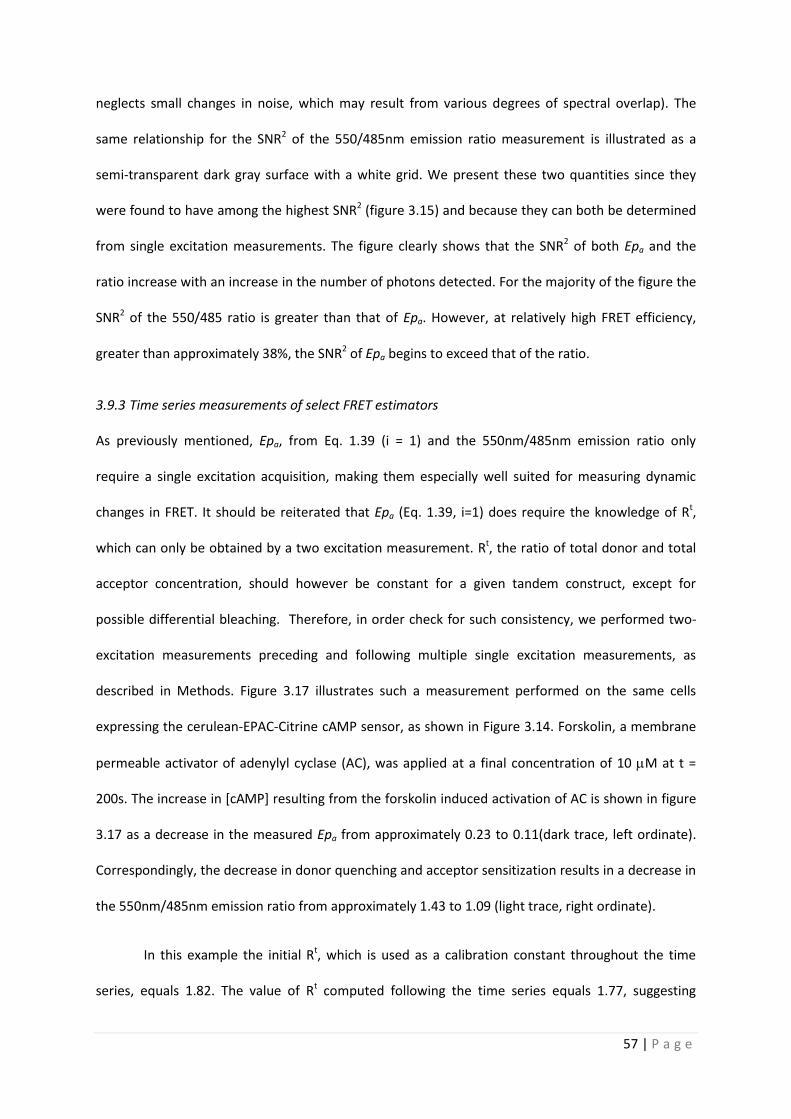
described in Methods. Figure 3.17 illustrates such a measurement performed on the same cells
expressing the cerulean-EPAC-Citrine cAMP sensor, as shown in Figure 3.14. Forskolin, a membrane
permeable activator of adenylyl cyclase (AC), was applied at a final concentration of 10 M at t =
200s. The increase in [cAMP] resulting from the forskolin induced activation of AC is shown in figure
3.17 as a decrease in the measured Epa from approximately 0.23 to 0.11(dark trace, left ordinate).
Correspondingly, the decrease in donor quenching and acceptor sensitization results in a decrease in
the 550nm/485nm emission ratio from approximately 1.43 to 1.09 (light trace, right ordinate).
In this example the initial Rt, which is used as a calibration constant throughout the time
series, equals 1.82. The value of Rt computed following the time series equals 1.77, suggesting
58 | P a g e
relatively little differential bleaching. The total acceptor concentration, At, changes from 1.17 to
1.09, indicating that approximately 7% of the 60% change measured in Epa results from acceptor
bleaching. The total donor concentration changes from 0.64 to 0.62 fold that of the donor reference
concentration throughout the course of the measurement and only influences Epa indirectly through
the differential bleaching present in Rt.
Figure 3.17 | Time course of Epa and the 550/485nm emission ratio. Multiple single excitation measurements
of cells expressing the cerulean-EPAC-citirine cAMP sensor shown in figures 1 and 2 were performed after an
initial two-excitation measurement. Forskolin was applied to a final concentration of 10M at t = 200 seconds.
A) The values calculated for Epa and the 550/485nm ratio are plotted over time as solid and dashed lines,
respectively. Note the different scales for the two quantities.
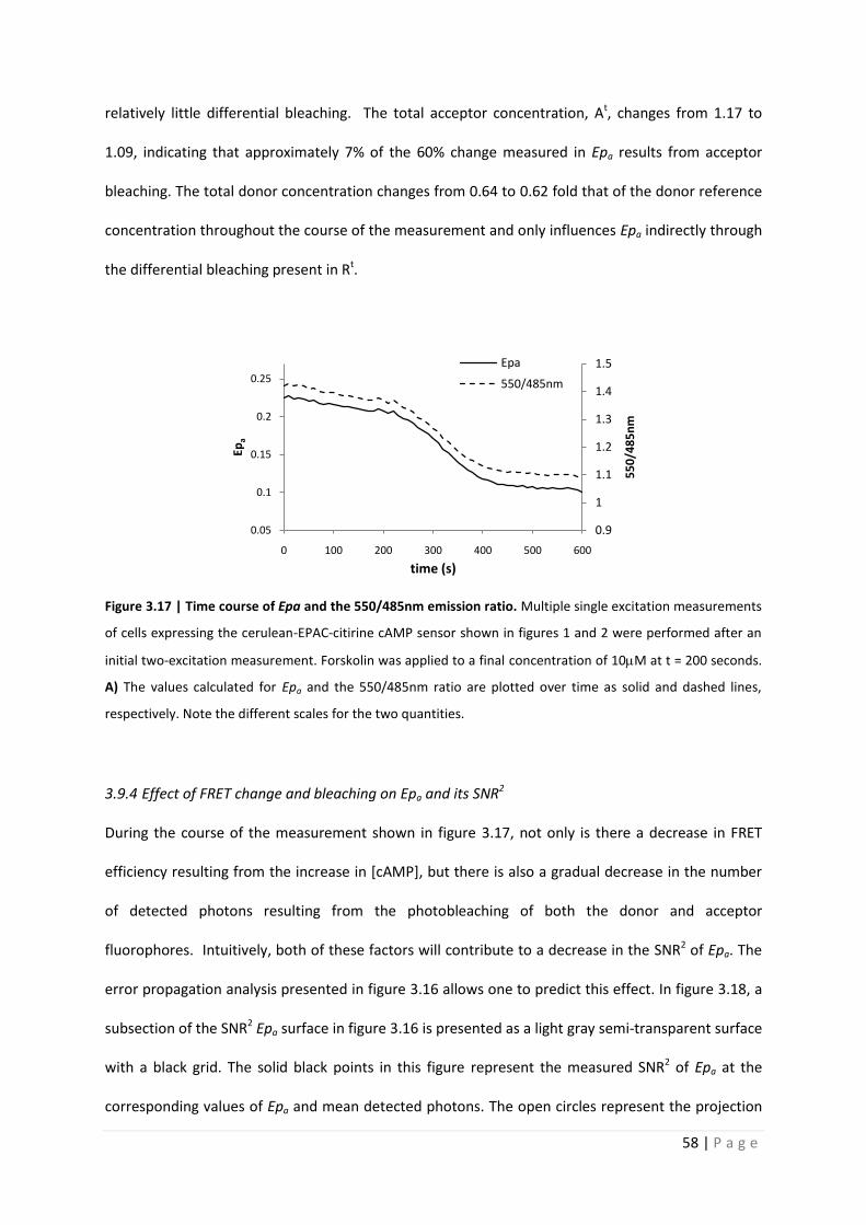
3.9.4 Effect of FRET change and bleaching on Epa and its SNR2
During the course of the measurement shown in figure 3.17, not only is there a decrease in FRET
efficiency resulting from the increase in [cAMP], but there is also a gradual decrease in the number
of detected photons resulting from the photobleaching of both the donor and acceptor
fluorophores. Intuitively, both of these factors will contribute to a decrease in the SNR2 of Epa. The
error propagation analysis presented in figure 3.16 allows one to predict this effect. In figure 3.18, a
subsection of the SNR2 Epa surface in figure 3.16 is presented as a light gray semi-transparent surface
with a black grid. The solid black points in this figure represent the measured SNR2 of Epa at the
corresponding values of Epa and mean detected photons. The open circles represent the projection
0.9
1
1.1
1.2
1.3
1.4
1.5
0.05
0.1
0.15
0.2
0.25
0 100 200 300 400 500 600
55
0/4
85
nm
Epa
time (s)
Epa
550/485nm
59 | P a g e
of each sampled measurement onto the prediction surface. Twelve equally spaced samples from the
time course measurement are plotted to illustrate the trend. This figure shows that the decrease
both in FRET efficiency and in the number of detected photons over time, results in a decreased
SNR2 of Epa that is quite well predicted by theory.
Figure 3.18 | Change in SNR2 of Epa over multiple measurements. Twelve points were sampled, in fifty second
intervals, from the Epa measurements presented in Panel A. The SNR2 of these measurements were plotted as
solid points against the corresponding FRET efficiency and number of detected photons. The gray surface is a
subsection of the surface presented in figure 4B and represents the relationship between SNR2 of Epa, FRET
efficiency, and number of detected photons as predicted from the error propagation analysis. The open circles
represent the projection of each sampled measurement onto the prediction surface.
3.9.5 Estimation of Ligand concentration
Measurements, such as those presented thus far, are often used only to indicate relative changes in
the concentration of a ligand, in this case [cAMP]. However, it is possible to estimate the absolute
ligand concentration from measurements, if the maximum and minimum FRET efficiencies (Emax and
Eo), corresponding to the sensor in its free and bound states are known, together with the Hill
coefficient and the dissociation constant. Likewise, [cAMP] can be calculated from the simple
emission ratio, if the corresponding maximum and minimum ratios are known (Grynkiewicz et al.
1985). Literature values for the Kd of this construct vary greatly (Ponsioen et al. 2004; Salonikidis et
60 | P a g e
al. 2008), so no absolute estimate was made. From now on [cAMP]/Kd will be designated as
[cAMP]*. For the following discussion we assume, for simplicity, that pa,i = 1 and bleaching to be
negligible. In the case of the Cerulean-EPAC-Citrine FRET sensor, Efree = 0.23, Ebound = 0.45, and Hill
coefficient n = 0.99 (Salonikidis et al submitted). The 550/485nm emission ratios expected on our
microscope that correspond to the free and bound states of the sensor were determined from the
corresponding FRET efficiencies and found to be 1.44 and 0.95, respectively. The error propagation
resulting from the conversion of FRET efficiency into ligand concentration is described by eq. 1.50.
Eq. 1.51 describes the error propagation resulting from the conversion of emission ratio into ligand
concentration. Maps of [cAMP]* were computed from the Epa and 550/485nm ratio maps. The SNR2
was calculated as previously discussed.
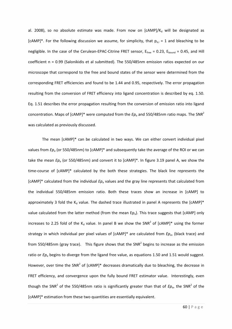
The mean [cAMP]* can be calculated in two ways. We can either convert individual pixel
values from Epa (or 550/485nm) to [cAMP]* and subsequently take the average of the ROI or we can
take the mean Epa (or 550/485nm) and convert it to [cAMP]*. In figure 3.19 panel A, we show the
time-course of [cAMP]* calculated by the both these strategies. The black line represents the
[cAMP]* calculated from the individual Epa values and the gray line represents that calculated from
the individual 550/485nm emission ratio. Both these traces show an increase in [cAMP] to
approximately 3 fold the Kd value. The dashed trace illustrated in panel A represents the [cAMP]*
value calculated from the latter method (from the mean Epa). This trace suggests that [cAMP] only
increases to 2.25 fold of the Kd value. In panel B we show the SNR2 of [cAMP]* using the former
strategy in which individual per pixel values of [cAMP]* are calculated from Epa, (black trace) and
from 550/485nm (gray trace). This figure shows that the SNR2 begins to increase as the emission
ratio or Epa begins to diverge from the ligand free value, as equations 1.50 and 1.51 would suggest.
However, over time the SNR2 of [cAMP]* decreases dramatically due to bleaching, the decrease in
FRET efficiency, and convergence upon the fully bound FRET estimator value. Interestingly, even
though the SNR2 of the 550/485nm ratio is significantly greater than that of Epa, the SNR2 of the
[cAMP]* estimation from these two quantities are essentially equivalent.
61 | P a g e
Figure 3.19 | Time course of the estimated cAMP concentration. With the knowledge of certain calibration
parameters the absolute ligand concentration can be readily calculated. A) The solid black line represents the
mean of the per pixel [cAMP]* values, derived from the per pixel Epa values. The dashed line corresponds to a
similar measurement with the [cAMP]* map calculated from the per pixel 550/485nm ratio values. The solid
gray line represents a case in which error propagation is neglected and the mean [cAMP]* calculated using the
mean Epa. B) The solid and dashed lines represent the SNR2 of the measurements from the [cAMP]* maps
based on Epa and 550/485nm emission ratio, respectively, over time. C) The relationship between the SNR2 of
the [cAMP]*, the FRET efficiency of the sensor, and the number of detected photons is represented by the
gray surface. The black points indicate the individual estimates from the measurements of the time series. This
figure shows, similarly to figure 4B, that the error propagation model accurately predicts the expected SNR2.
Part C of the figure shows the relationship between the number of detected photons, the
FRET efficiency of the sensor, and the SNR2 of the [cAMP]* estimate, derived from our error
0
1
2
3
4
5
6
7
8
0 200 400 600
[cA
MP
]*
time (s)
Epa
550/485nm
mean Epa
0
0.5
1
1.5
2
0 200 400 600
SNR
2 [c
AM
P]*
time (s)
Epa550/485nm
A B
C
62 | P a g e
propagation analysis using eq. 1.50. The black points indicate the time course of our measurement.
This figure shows, similarly to figure 3.18 that our error propagation model accurately predicts the
expected SNR2. It clearly shows the increase in SNR2 of the [cAMP]* estimate as the FRET efficiency
decreases from that of the ligand free state. As equation 1.50 suggests, this figure also shows that
the SNR2 (1/CV2) decreases to 0 when FRET efficiency begins to approach that of the bound state.
Also, as would be expected, the model indicates the coordinated decrease of the SNR2 of [cAMP]*
with that of the number of detected photons.
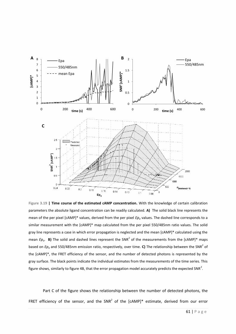
3.9.6 Biasing resulting from Error propagation
In figure 3.19 we see that the apparent running average of the mean [cAMP]* measured from the
per pixel conversion is greater than the [cAMP]* converted from the mean Epa. The reason for this
discrepancy was not immediately clear, so a closer look was taken. It is reasonable to assume that
negative [cAMP]* values could be calculated due to error propagation, although negative
concentration is not physically possible. If these pixels were not allowed in the analysis and set to
zero or neglected, the mean calculated over the ROI would be greater and contain less noise than it
should. To show that negative values are in fact allowed and used in the computation of mean
[cAMP]*, the distributions of pixel [cAMP]* values are presented for multiple time points (and FRET
efficiencies) in figure 3.20.
Not only do these distributions show that negative pixels are used in the computation of
mean [cAMP]* but they also clearly indicate the increase in noise over time. The shape of the
distributions indicate that either there is a low [cAMP]* cut-off (possibly resulting from intensity
thresholding) or there is a significant skew in the distributions. No cut-off was used in the analysis.
Furthermore the cut off required to explain the shape of the distribution seems to change over time
suggesting that the distributions are rather skewed.
63 | P a g e
Figure 3.20 | Distribution of [cAMP]* values within the sampled ROI. Histograms of per pixel values are
plotted from the same ROI used in the previous analysis. Panel A represents the [cAMP]* distribution at 100
seconds when Epa is approximately 0.22. This distribution shows that negative values exist and are used in the
computation of mean and error of [cAMP]* within the ROI. Panel C represents the [cAMP]* distribution at
600s when Epa is approximately 0.11. The intermediate panel (B) illustrates the [cAMP]* distribution at t =
300s.
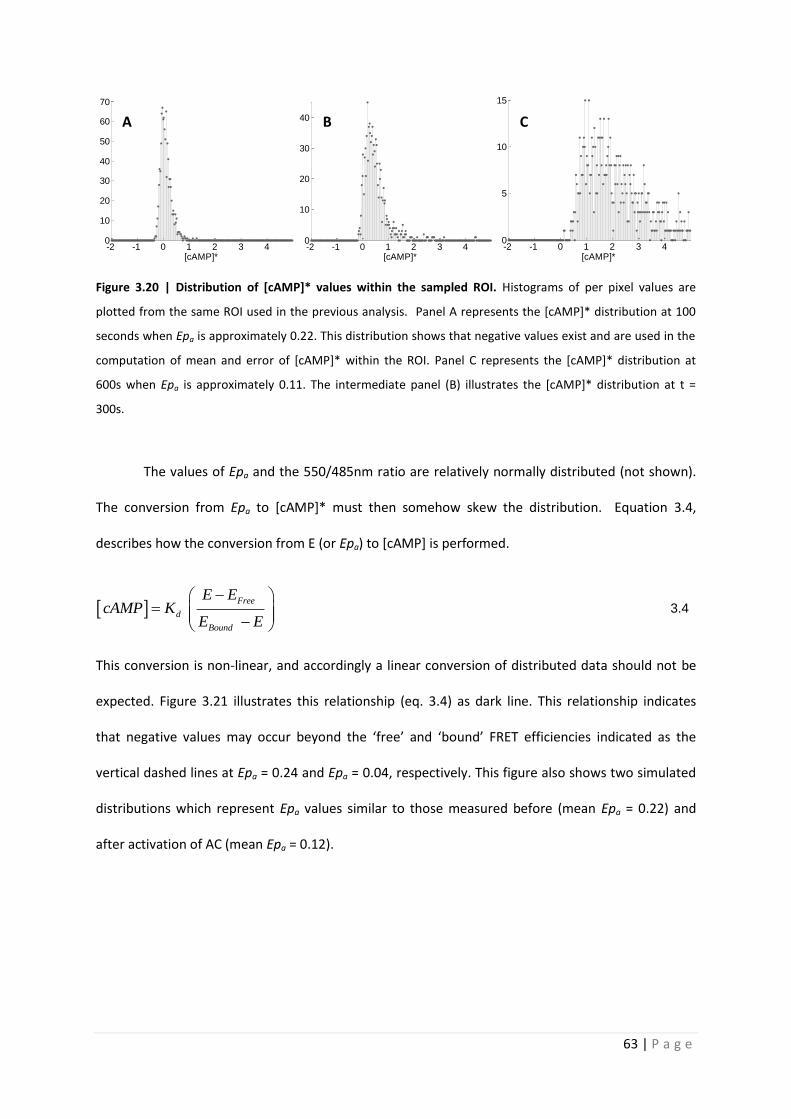
The values of Epa and the 550/485nm ratio are relatively normally distributed (not shown).
The conversion from Epa to [cAMP]* must then somehow skew the distribution. Equation 3.4,
describes how the conversion from E (or Epa) to [cAMP] is performed.
Free
d
Bound
E EcAMP K
E E
3.4
This conversion is non-linear, and accordingly a linear conversion of distributed data should not be
expected. Figure 3.21 illustrates this relationship (eq. 3.4) as dark line. This relationship indicates
that negative values may occur beyond the ‘free’ and ‘bound’ FRET efficiencies indicated as the
vertical dashed lines at Epa = 0.24 and Epa = 0.04, respectively. This figure also shows two simulated
distributions which represent Epa values similar to those measured before (mean Epa = 0.22) and
after activation of AC (mean Epa = 0.12).
-2 -1 0 1 2 3 40
10
20
30
40
50
60
70
[cAMP]*-2 -1 0 1 2 3 40
10
20
30
40
[cAMP]*-2 -1 0 1 2 3 40
5
10
15
[cAMP]*
A B C
64 | P a g e
Figure 3.21 | Conversion from Epa to [cAMP]*. A) The dark black trace indicates the [cAMP]* as a function of E
described by Eq. 3.5 (left ordinate). The dashed vertical lines at Epa = 0.04 and Epa = 0.24 correspond the
‘bound’ and ‘free’ state Epa values, respectively. The dashed distribution simulates the Epa expected at low
concentrations of [cAMP] with the mean Epa = 0.22. The gray distribution simulates the expected Epa
distribution of Epa at elevated [cAMP] when the mean Epa = 0.12. B) The dashed and gray [cAMP]* distribution
correspond to the dashed and gray Epa distribution in the previous figure.
By projecting the Epa distributions in figure 3.21 onto the line representing the E to [cAMP]*
conversion we can convert them to corresponding distributions of [cAMP]*. Figure 3.21 panel B
shows that this conversion skews normally distributed E data from figure 3.21 panel A. This is most
apparent with the gray distribution which corresponds to low Epa (high [cAMP]). The greater skew in
the high [cAMP]* arises from the overlap of the low Epa distribution with a more non-linear region of
the conversion function. In the case of a linear conversion we would expect an increase or decrease
the standard deviation corresponding to a change in units however no skew in the data should
-1
-0.5
0
0.5
1
1.5
-10
-5
0
5
10
15
-0.1 0 0.1 0.2 0.3
a.u
.
[cA
MP
]*
Epa
0
0.2
0.4
0.6
0.8
1
1.2
-1 0 1 2 3 4 5
a.u
.
[cAMP]*
A
B
65 | P a g e
occur. It should be noted that these distributions correspond quite well with those measured at
comparable Epa values (first and last panels of figure 3.20).
3.9.7 Comparison of dynamic range to noise
The ability of Epa and the 550/485nm ratio to be converted to [cAMP]* with the same SNR suggests
that either the error propagation for Epa is more favorable than that of the emission ratio or that the
SNR of these parameters insufficiently characterizes their ability to resolve changes in FRET. In such
a case the SNR of these quantities would not directly comparable. The equations used to convert Epa
and the emission ratio to [cAMP] were derived analogously and propagate error accordingly.
Comparing the Epa and 550/485nm images in figure 3.14 the images appear to have similar levels of
noise, with the color bars appropriately and proportionally scaled. However, we see in figure 3.15
that the SNR measured from the images differ greatly with SNR of Epa equal to 7.95 and the SNR of
the emission ratio equal to 15.89. As was discussed earlier, SNR is unitless and scale invariant, it is
not however offset invariant. If the amount of noise in two quantities is similar but one quantity has
a higher basal level or offset it will also have a higher SNR, regardless of the response amplitude or
dynamic range. In the case of the 550/485nm emission ratio, at E = 0, a signal of approximately 0.8 is
measured. In this case what becomes important is not the amount of noise relative to the basal level
or even absolute value, but the amount of noise relative to response from a change in FRET.
The relative change in a parameter can be calculated by dividing the deviation from the
parameters mean initial value by this mean initial value. This normalizes all quantities to an initial
value of one and allows us to more appropriately compare the relative dynamic ranges of each
computed quantity. When this normalization is performed on a per pixel basis, using the mean initial
value defined from a region of interest, it allows for the quantification of noise relative to this
normalized value. This calculation was performed for the 550/485nm emission ratio, the apparent
concentration ratio, and Epa in the example of the change in [cAMP]* shown above. A mean of
these quantities was sampled form the same ROI used in the previous examples. Figure 3.22 below
66 | P a g e
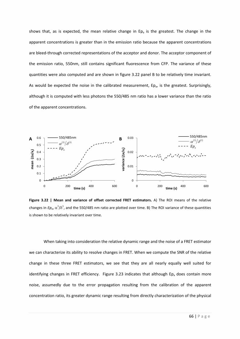
shows that, as is expected, the mean relative change in Epa is the greatest. The change in the
apparent concentrations is greater than in the emission ratio because the apparent concentrations
are bleed-through corrected representations of the acceptor and donor. The acceptor component of
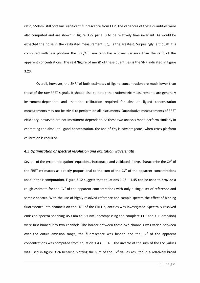
the emission ratio, 550nm, still contains significant fluorescence from CFP. The variance of these
quantities were also computed and are shown in figure 3.22 panel B to be relatively time invariant.
As would be expected the noise in the calibrated measurement, Epa, is the greatest. Surprisingly,
although it is computed with less photons the 550/485 nm ratio has a lower variance than the ratio
of the apparent concentrations.
Figure 3.22 | Mean and variance of offset corrected FRET estimators. A) The ROI means of the relative
changes in Epa, 1/
1, and the 550/485 nm ratio are plotted over time. B) The ROI variance of these quantities
is shown to be relatively invariant over time.
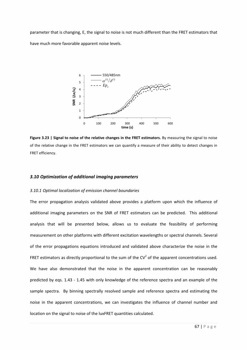
When taking into consideration the relative dynamic range and the noise of a FRET estimator
we can characterize its ability to resolve changes in FRET. When we compute the SNR of the relative
change in these three FRET estimators, we see that they are all nearly equally well suited for
identifying changes in FRET efficiency. Figure 3.23 indicates that although Epa does contain more
noise, assumedly due to the error propagation resulting from the calibration of the apparent
concentration ratio, its greater dynamic range resulting from directly characterization of the physical
0
0.1
0.2
0.3
0.4
0.5
0.6
0 200 400 600
me
an (
x/x i
)
time (s)
550/485nm
a(1)/d(1)
Epa
0
0.01
0.02
0.03
0 200 400 600
vari
ance
(
x/x i
)
time (s)
550/485nm
a(1)/d(1)
Epa
A B 1 1
1 1
aEp aEp
67 | P a g e
parameter that is changing, E, the signal to noise is not much different than the FRET estimators that
have much more favorable apparent noise levels.
Figure 3.23 | Signal to noise of the relative changes in the FRET estimators. By measuring the signal to noise
of the relative change in the FRET estimators we can quantify a measure of their ability to detect changes in
FRET efficiency.
3.10 Optimization of additional imaging parameters
3.10.1 Optimal localization of emission channel boundaries
The error propagation analysis validated above provides a platform upon which the influence of
additional imaging parameters on the SNR of FRET estimators can be predicted. This additional
analysis that will be presented below, allows us to evaluate the feasibility of performing
measurement on other platforms with different excitation wavelengths or spectral channels. Several
of the error propagations equations introduced and validated above characterize the noise in the
FRET estimators as directly proportional to the sum of the CV2 of the apparent concentrations used.
We have also demonstrated that the noise in the apparent concentration can be reasonably
predicted by eqs. 1.43 - 1.45 with only knowledge of the reference spectra and an example of the
sample spectra. By binning spectrally resolved sample and reference spectra and estimating the
noise in the apparent concentrations, we can investigates the influence of channel number and
location on the signal to noise of the luxFRET quantities calculated.
0
1
2
3
4
5
6
0 100 200 300 400 500 600
SNR
(
x/x i
)
time (s)
550/485nm
a(1)/d(1)
Epa
1 1
aEp
68 | P a g e
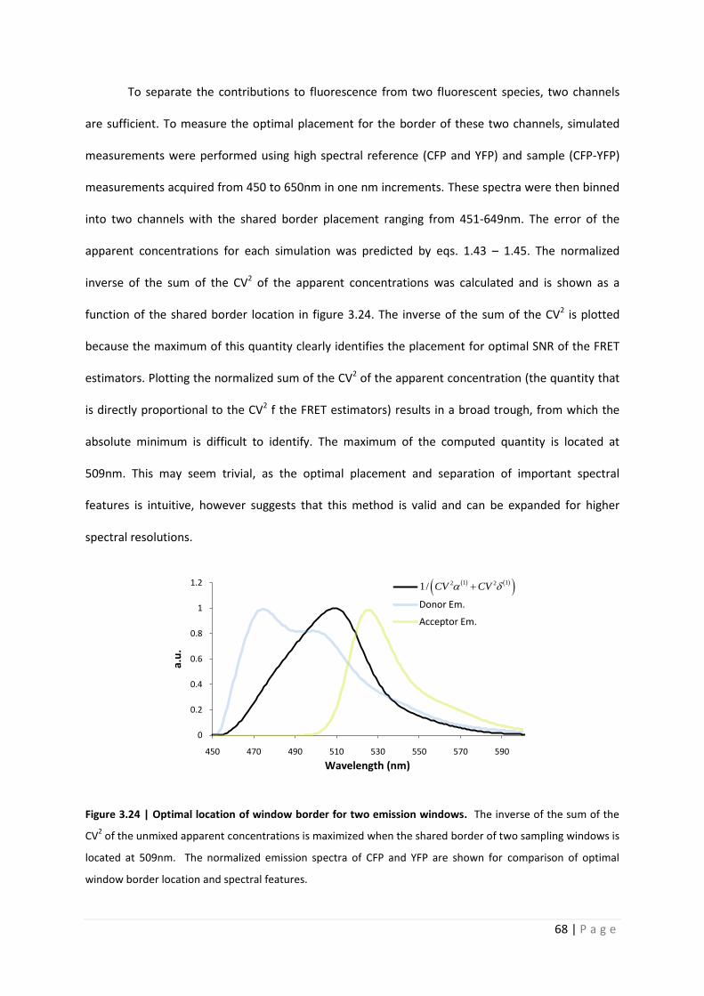
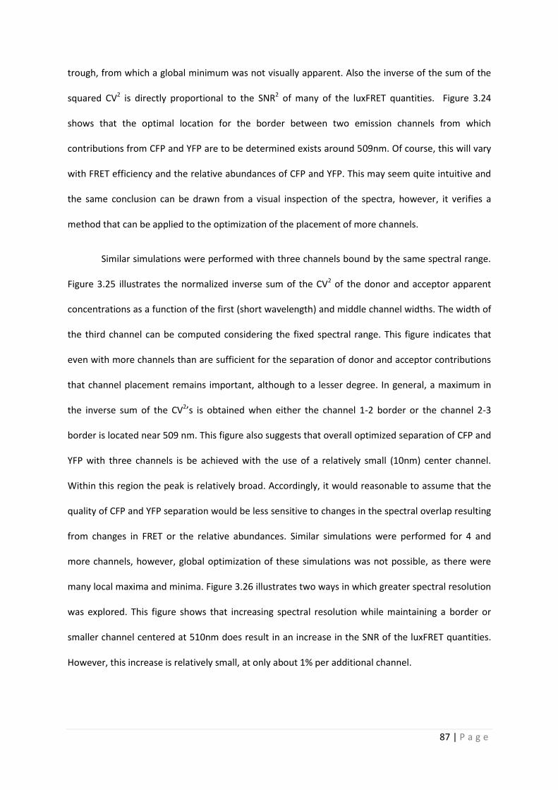
To separate the contributions to fluorescence from two fluorescent species, two channels
are sufficient. To measure the optimal placement for the border of these two channels, simulated
measurements were performed using high spectral reference (CFP and YFP) and sample (CFP-YFP)
measurements acquired from 450 to 650nm in one nm increments. These spectra were then binned
into two channels with the shared border placement ranging from 451-649nm. The error of the
apparent concentrations for each simulation was predicted by eqs. 1.43 – 1.45. The normalized
inverse of the sum of the CV2 of the apparent concentrations was calculated and is shown as a
function of the shared border location in figure 3.24. The inverse of the sum of the CV2 is plotted
because the maximum of this quantity clearly identifies the placement for optimal SNR of the FRET
estimators. Plotting the normalized sum of the CV2 of the apparent concentration (the quantity that
is directly proportional to the CV2 f the FRET estimators) results in a broad trough, from which the
absolute minimum is difficult to identify. The maximum of the computed quantity is located at
509nm. This may seem trivial, as the optimal placement and separation of important spectral
features is intuitive, however suggests that this method is valid and can be expanded for higher
spectral resolutions.
Figure 3.24 | Optimal location of window border for two emission windows. The inverse of the sum of the
CV2 of the unmixed apparent concentrations is maximized when the shared border of two sampling windows is
located at 509nm. The normalized emission spectra of CFP and YFP are shown for comparison of optimal
window border location and spectral features.
0
0.2
0.4
0.6
0.8
1
1.2
450 470 490 510 530 550 570 590
a.u
.
Wavelength (nm)
1/(CV2a+CV2d)
Donor Em.
Acceptor Em.
1 12 21/ CV CV
69 | P a g e
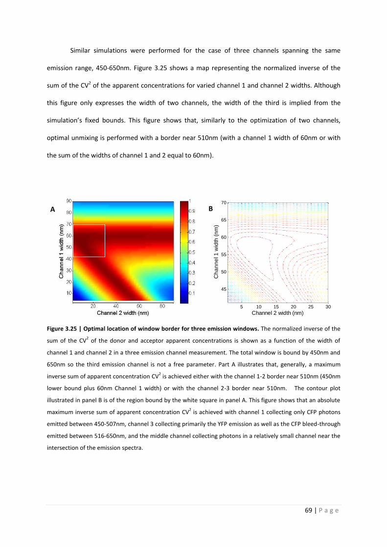
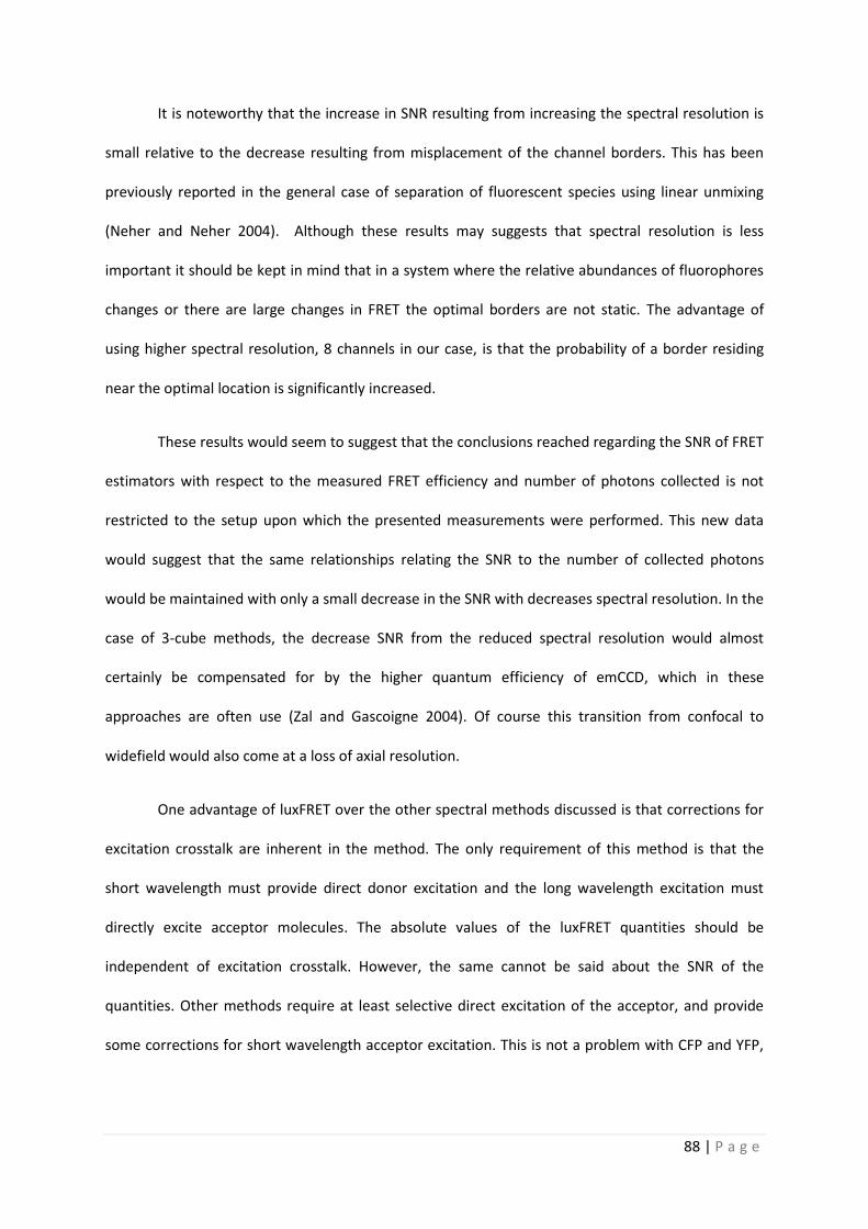
Similar simulations were performed for the case of three channels spanning the same
emission range, 450-650nm. Figure 3.25 shows a map representing the normalized inverse of the
sum of the CV2 of the apparent concentrations for varied channel 1 and channel 2 widths. Although
this figure only expresses the width of two channels, the width of the third is implied from the
simulation’s fixed bounds. This figure shows that, similarly to the optimization of two channels,
optimal unmixing is performed with a border near 510nm (with a channel 1 width of 60nm or with
the sum of the widths of channel 1 and 2 equal to 60nm).
Figure 3.25 | Optimal location of window border for three emission windows. The normalized inverse of the
sum of the CV2 of the donor and acceptor apparent concentrations is shown as a function of the width of
channel 1 and channel 2 in a three emission channel measurement. The total window is bound by 450nm and
650nm so the third emission channel is not a free parameter. Part A illustrates that, generally, a maximum
inverse sum of apparent concentration CV2 is achieved either with the channel 1-2 border near 510nm (450nm
lower bound plus 60nm Channel 1 width) or with the channel 2-3 border near 510nm. The contour plot
illustrated in panel B is of the region bound by the white square in panel A. This figure shows that an absolute
maximum inverse sum of apparent concentration CV2 is achieved with channel 1 collecting only CFP photons
emitted between 450-507nm, channel 3 collecting primarily the YFP emission as well as the CFP bleed-through
emitted between 516-650nm, and the middle channel collecting photons in a relatively small channel near the
intersection of the emission spectra.
Channel 2 width (nm)
Ch
an
ne
l 1
wid
th (
nm
)
5 10 15 20 25 30
45
50
55
60
65
70
A B
70 | P a g e
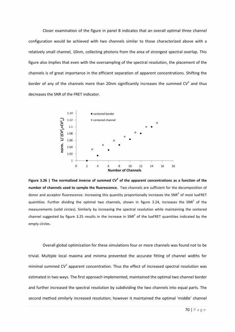
Closer examination of the figure in panel B indicates that an overall optimal three channel
configuration would be achieved with two channels similar to those characterized above with a
relatively small channel, 10nm, collecting photons from the area of strongest spectral overlap. This
figure also implies that even with the oversampling of the spectral resolution, the placement of the
channels is of great importance in the efficient separation of apparent concentrations. Shifting the
border of any of the channels more than 20nm significantly increases the summed CV2 and thus
decreases the SNR of the FRET indicator.
Figure 3.26 | The normalized inverse of summed CV2 of the apparent concentrations as a function of the
number of channels used to sample the fluorescence. Two channels are sufficient for the decomposition of
donor and acceptor fluorescence. Increasing this quantity proportionally increases the SNR2 of most luxFRET
quantities. Further dividing the optimal two channels, shown in figure 3.24, increases the SNR2 of the
measurements (solid circles). Similarly by increasing the spectral resolution while maintaining the centered
channel suggested by figure 3.25 results in the increase in SNR2 of the luxFRET quantities indicated by the
empty circles.
Overall global optimization for these simulations four or more channels was found not to be
trivial. Multiple local maxima and minima prevented the accurate fitting of channel widths for
minimal summed CV2 apparent concentration. Thus the effect of increased spectral resolution was
estimated in two ways. The first approach implemented, maintained the optimal two channel border
and further increased the spectral resolution by subdividing the two channels into equal parts. The
second method similarly increased resolution; however it maintained the optimal ‘middle’ channel
1
1.02
1.04
1.06
1.08
1.1
1.12
1.14
0 2 4 6 8 10 12 14 16 18
no
rm.
1/
(CV
2 +C
V2)
Number of Channels
centered border
centered channel
71 | P a g e
defined by the three channel optimization. Figure 3.26 shows the 1/CV2 relative to the optimal two
channel measurement. This figure clearly indicates an increase in the SNR of the FRET estimators
with increased spectral resolution, with the centered border and centered channel estimates
converging when more than 10 channels are used (at a spectral resolution of 20nm/channel).
However, surprisingly, the increase is only approximately 1% SNR2 per additional channel. This is
relatively low compared to the decrease in SNR2 resulting from the misplacement of the channel
border in the two channel measurement.
3.10.2 Optimization of excitation wavelengths
Noise propagation through the spectral FRET analysis was also investigated through Monte Carlo
simulations. Emission from a sample with a given FRET efficiency was simulated through the use of
measured reference spectra and equation 1.12. Noise was added to the sample corresponding to
shot noise from a given number of collected photons. These simulations allow for predictions similar
to those made by the error propagation analysis. Additionally these simulations provide a method
through with other predictions can be made.
One advantageous feature of the spectral analysis presented above is the ability of the
method to be applied without additional corrections for or absolute criteria for excitation crosstalk.
Other quantitative spectral methods require a long wavelength excitation that does not excite any
donor molecules. This is not a problem for CFP-YFP. However, with other FRET pairs an appropriate
excitation source may not be available. Although luxFRET allows for virtually any excitation
wavelengths to be used, we have shown that the use of certain excitation wavelengths can simplify
the analysis performed, generally through the assumption of negligible donor excitation with the
long-wavelength excitation, allowing one to set rex,2 equal to 0. It is reasonable to assume that,
although the analysis is possible and may yield the correct results at any pair of excitation
wavelengths, that the noise may be affected. To further explore this we used the discussed
simulations to predict the SNR2 of EfD and EfA for a range of paired excitation wavelengths. To do
72 | P a g e
this, however, the ratio of extinction coefficients, which are usually determined empirically in the
calibration steps of the luxFRET analysis, and for which measured values were used in the initial
evaluation of the simulations, must be estimated. Reasonable estimates for these ratios can be
gathered from literature, however, due to the impracticality of accurately characterizing the spectral
properties of one’s excitation source they should not be used in place of empirically determined
values when available.
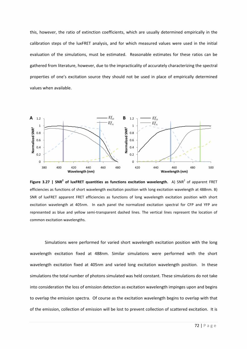
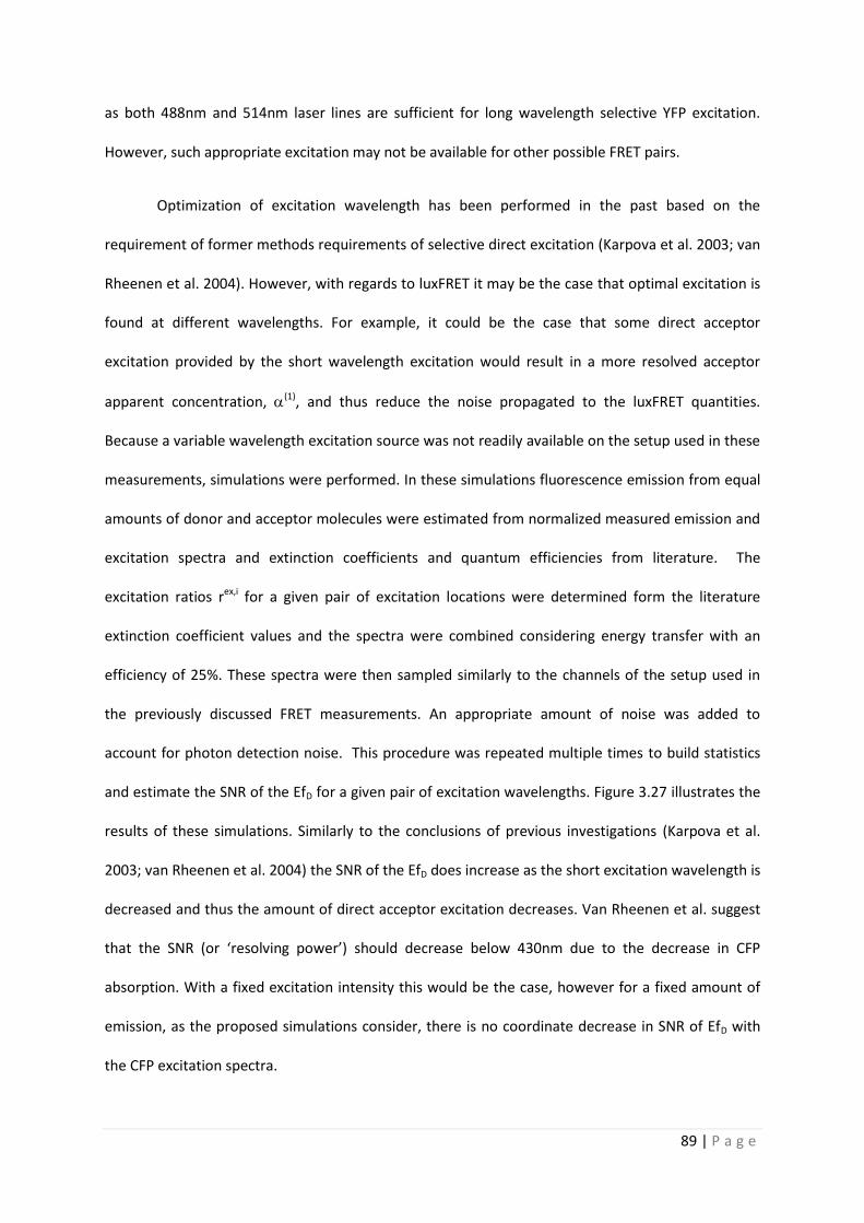
Figure 3.27 | SNR2 of luxFRET quantities as functions excitation wavelength. A) SNR
2 of apparent FRET
efficiencies as functions of short wavelength excitation position with long excitation wavelength at 488nm. B)
SNR of luxFRET apparent FRET efficiencies as functions of long wavelength excitation position with short
excitation wavelength at 405nm. In each panel the normalized excitation spectral for CFP and YFP are
represented as blue and yellow semi-transparent dashed lines. The vertical lines represent the location of
common excitation wavelengths.
Simulations were performed for varied short wavelength excitation position with the long
wavelength excitation fixed at 488nm. Similar simulations were performed with the short
wavelength excitation fixed at 405nm and varied long excitation wavelength position. In these
simulations the total number of photons simulated was held constant. These simulations do not take
into consideration the loss of emission detection as excitation wavelength impinges upon and begins
to overlap the emission spectra. Of course as the excitation wavelength begins to overlap with that
of the emission, collection of emission will be lost to prevent collection of scattered excitation. It is
0
0.2
0.4
0.6
0.8
1
1.2
380 400 420 440 460 480
No
rmal
ize
d S
NR
2
Wavelength (nm)
EfD
EfA
0
0.2
0.4
0.6
0.8
1
1.2
420 440 460 480 500
No
rmal
ize
d S
NR
2
Wavelength (nm)
EfD
EfA
A B DEfDEf
AEfAEf
73 | P a g e
reasonable to assume that as the excitation wavelength shown in figure 3.27 approaches the onset
of CFP emission, approximately 450nm, that a steeper decrease in actual SNR2 would occur. Of
course this would not be due to the value of excitation ratio, rex,1, but rather due to the loss in
collected photons due to appropriate emission channel placement. As was shown in the error
propagation analysis, the SNR2 of EfD is greater than that of EfA. As would be expected the SNR of
these two quantities vary differently with either excitation wavelength. EfA is determined completely
from acceptor emission. Figure 3.27 panel B clearly shows that as the excitation 2 wavelength
decreases and a contribution to fluorescence from CFP is measured the SNR of EFA rapidly decreases.
This contribution to fluorescence from CFP (non-negligible 2) results in a decreased SNR of 2. As
neither EfD nor EfA are functions of 2, neither quantity increase in SNR with shorter wavelength
excitation 2 measurements.
The results of the simulations were verified with measurements performed at three
different wavelengths. 10 N1E cells expressing the CFP-YFP tandem construct were imaged at
405nm, 458nm, and 488nm. Three sets of FRET estimators were calculated with each combination of
the three excitations. Figure 3.27 panel A shows the SNR2 of the 405nm/488nm measurement as a
function of the corresponding 458nm/488nm measurement. Cells with different concentrations and
varied excitation intensities were used such that the total collected photons measured varied
between 618 and 2,834, resulting in a spread in the data. The data was fit with a linear regression
indicating that the SNR2 of EfD when using 405nm as the short excitation is 1.37 fold of that when
using 458nm as a short excitation wavelength. Interestingly, even though the SNR of (1) can be
assumed to be less due to a lesser degree of direct excitation, the use of 405nm as the excitation 1
wavelength results in an even more augmented SNR2 of Efa (1.74 fold). One can postulate that this is
due to the greater fraction of 1 resulting from sensitized emission, and thus containing more direct
information about the FRET efficiency. Comparing these data to those predicted we see that the
general relationship between the values is the same however the simulations predicted even larger
increases in SNR2 for EfD and EfA, 1.6 and 2.2 fold, respectively.
74 | P a g e
The simulations predict that the use of 458nm would result in a SNR2 of EfD of 94% that of
the same measurement with excitation 2 at 488nm. The measurements are in good agreement, with
the SNR2 of EfD with long wavelength excitation at 458nm being 92% that of at 488nm. The
predictions for EfA do not match the measurements as accurately. The simulations predict that the
use of 458nm as the long wavelength excitation would decrease the SNR2 of EfA to only 23% that of
the case in which 488nm is used. The measurements indicate that the decrease is much more
severe, with the SNR2 effectively equal to zero for all measurements.
Figure 3.28 | Comparison of resulting SNR2 of apparent FRET efficiencies with varied Ex1 and Ex2
wavelengths. A) In the case that 405nm is used as the short wavelength excitation, rather than 458nm, an
increase in the SNR2 of EFD of 1.37 fold in measured. In the case of the SNR2 of EfA an increase of 1.74 is
measured. B) In the case that 458nm is used as the long wavelength excitation, rather than 488nm, a decrease
of 0.92 fold is expected for the SNR2 of EfD. The SNR
2 of EfA for all of the the 405/458nm measurements are
more or less equal to 0.
y = 1.37x
y = 1.74x
0
20
40
60
80
100
120
0 20 40 60 80
SNR
24
05
nm
/48
8n
m
SNR2 458nm/488nm
EfDEfA
y = 0.92x
y = 0.0011x
0
20
40
60
80
100
120
0 25 50 75 100
SNR
24
05
nm
/45
8n
m
SNR2 405nm/488nm
EfDEfA
A B
75 | P a g e
4 Discussion
4.1 Implementation and validation of a novel spectral FRET method
In the preceding a method for spectral analysis of FRET-signals was presented. The equations
derived to characterize FRET take into consideration both the contributions of unpaired donor and
acceptor fluorophores and the influence of incomplete labeling of the interacting partners. In this
method the contributions to fluorescence from a FRET sample measured at two different excitation
wavelengths are separated using linear unmixing with donor and acceptor reference spectra. The
weights of these reference spectra defined during the unmixing procedure, denoted apparent
concentrations, are used along with calibration constants to determine two apparent FRET
efficiencies. These apparent FRET efficiencies correspond to those measured from donor quenching
and acceptor sensitization-type experiments. In addition to the apparent FRET efficiencies we also
determine the FRET-corrected total donor and total acceptor concentrations (as factors of the
reference concentrations). These total concentrations are used to determine the FRET-corrected
total acceptor to total donor ratio. Furthermore these derivations suggest that spectral analysis of
intermolecular FRET cannot yield accurate values of the Förster energy transfer efficiency E, unless
one of the interactors is in large excess and perfectly labeled. In the case of imperfect labeling or
intermolecular FRET with free donor and acceptors spectral analysis yield the products EfD and EfA
where fD and fA represent the fraction of donor or acceptors participating in the FRET complex, also
referred to as fractional occupancies.
To verify that the values determined by the presented method were accurate, a CFP-YFP
tandem construct was used as a FRET standard and luxFRET measurements were compared to those
from established methods. The first method used to verify the apparent FRET efficiency determined
by the luxFRET analysis was acceptor photobleaching. This method directly compares the
fluorescence intensity of quenched donor in presence of acceptor with the intensity of the free
donor by removing the acceptor in the same sample through photobleaching. The effect of donor
76 | P a g e
quenching due to energy transfer can thus be directly calculated. Donor quenching was also
measured by quantifying the excited state lifetime of the FRET construct as well as that of the free
donor through time correlated single photon counting. Unlike the intensity of fluorescence emission
used in the acceptor photobleaching measurements, the excited state lifetime is concentration
independent so measurements can be performed on two different samples. The apparent FRET
efficiencies reported from these two methods (figure 3.3) as well as the proposed method (figure
3.2) were shown to be in good agreement.
A closer look was taken at the underlying factors which contribute to the fractions included
within the apparent FRET efficiencies. It was concluded that these fractions are composed of the
products fdpa and fapd’ , with pa,d denoting the probability that a given donor/acceptor interactor
molecule is labeled with an appropriate and functional fluorophore. The prime in pd’ serves as a
reminder that this quantity also depends on the folding/labeling state of the tandem construct used
in the calibration procedure (see eq. 1.36). In the case of fluorescent proteins the probabilities of
correct folding have been shown to depend on temperature and other ambient factors and have
been estimated to vary between 50 – 90% (Sugiyama et al. 2005; Yasuda et al. 2006). Most
fluorescent proteins must also undergo a post-translational maturation before they become
functional (Ogawa et al. 1995). This implies a time dependency of these probabilities. Differences in
the maturation half time between donor and acceptor molecules can lead to a time dependent
stoichiometry upon which a measured apparent FRET efficiency would depend.
4.2 Considerations for fluorophore bleaching and protonation
One problem that is not present in spectroscopy, as much as it is in microscopy, is photobleaching.
This photo-destructive process leads to time dependent changes in pa and pd’. The equations derived
in luxFRET suggest that each of the apparent FRET efficiencies measured is susceptible to
photobleaching of one of the species. Figure 3.4 show in the case of acceptor bleaching that the
quantity Efdpa decreases over time while Efapd remains constant. Accordingly the total acceptor to
77 | P a g e
total donor ratio decreases over time with increased bleaching. One advantage of the proposed
methods is that it allows one to quantify the total acceptor concentration of the FRET sample
(relative to the reference), from which the relative change in pa can be quantified. Using this, it is
shown in figure 3.4 panel D that the estimated Epa can be corrected for any time dependent changes
in pa and the quantity Epa,o, where pa,o is the initial time-independent labeling probability, can be
determined. This provides a basis upon which photobleaching dependent change in the apparent
FRET efficiencies can be corrected.
Others have proposed methods for correcting FRET measurements for acceptor bleaching
(Zal and Gascoigne 2004). Among the methods proposed, is the characterization of bleaching
kinetics from reference acceptor samples as well as the use of direct excitation of the acceptor in a
FRET sample to follow the decrease in concentration. This group as well as others takes into
consideration sensitized bleaching and FRET dependent acceptor bleaching kinetics and make
suggestions according to the type of experiment being performed (Mekler et al. 1997; Zal and
Gascoigne 2004). Although direct acceptor excitation measurements will provide sufficient
information for correcting EfD, it may be the case that direct excitation without excitation crosstalk
and emission bleed-through is not possible. In such a case, the detected emission would not
necessarily characterize the decrease in acceptor concentration. The calculation of the FRET
corrected total acceptor concentration, as performed in the luxFRET analysis, still allows for
bleaching correction with excitation crosstalk and emission bleedthrough.
Most of the GFP variants have been shown to exist in a balance between protonated and
non-protonated states. In the case of YFP, protonation has been shown to alter the fluorescent
properties of the chromophore such that it the absorption spectrum is blue shifted with a peak near
390nm (McAnaney et al. 2005). Absorption is shifted to such an extent that there is neither overlap
with the excitation wavelengths used nor with the donor emission spectrum. The protonated form
of YFP can be considered to exist in a dark state in the measurements performed herein. The pKa of
78 | P a g e
the protonation reaction is near physiological pH (Miyawaki et al. 1999), further complicating the
use of YFP in biological samples. This dependence has been shown to influence FRET measurements
such that quantitative calibrations may vary greatly between samples (Salonikidis et al. 2008). Figure
3.5 shows, similarly to the acceptor photobleaching experiments, that the quantity Efapd is nearly
independent of the pH dependent changes in YFP fluorescence, while Efdpa and Rt are affected. At
lower pH the fluorescence of CFP is influenced (Llopis et al. 1998) and would affect this Efapd’ and Rt,
however this occurs at an extreme for physiological pH so it is generally negligible in biological
samples. Although the pH dependence of GFP and its variants have found some use (Heim and Tsien
1996; Miesenbock et al. 1998; Abad et al. 2004; Esposito et al. 2008), in most FRET measurements
this dependence is unwanted and can prevent quantitative measurements. However, with a
dependent and independent quantity defined by luxFRET, not only is it possible to monitor the FRET
state of the system, but ambient factors to which one fluorophore is sensitive can be monitored
simultaneously.
4.3 Identification of intermolecular interaction
In the measurements performed thus far, only a CFP-YFP tandem construct has been used as a FRET
standard. Not only can the presented method also be applied to intermolecular FRET systems, but
the additional quantities it characterizes are pertinent to quantitatively assessing the level of
interaction between two species of molecules. The apparent FRET efficiencies that this and other
steady state methods quantify, are composed of the characteristic efficiency of energy transfer as
well as fractional occupancy of donor with acceptor, fD, or that of acceptor with donor, fA. These
fractional occupancies are in turn dependent on the relative abundances of donor and acceptor
present in the sample. Thus simultaneous characterization of both the apparent FRET efficiency as
well as some measure of the relative amounts of donor and acceptor (ratio or fraction) are
necessary to appropriately address questions regarding degrees of interaction.
79 | P a g e
To illustrate the application of this method to the identification of intermolecular
interaction, measurements were performed on three sets of receptors. CD-86 and CD-28 were used
as monomeric and dimeric membrane receptor controls, respectively (James et al. 2006; Dorsch et
al. 2009). The 5HT1A receptor was the sample for which interaction was being investigated.
Biochemical assays as well as some FRET measurements have suggest that this receptor forms
homo-oligomers in the plasma membrane (Kobe et al. 2008; Woehler et al. 2009). To compare
measurements between these samples, the apparent FRET efficiencies were plotted as functions of
the corresponding donor fraction measured in each sample in figure 3.6. As the fractional occupancy
terms contained within the apparent FRET efficiencies are dependent on the relative abundance of
acceptors and donors, comparison of efficiencies at the same expression ratio (or fraction) is
essential.
The apparent FRET efficiency measured from the samples expressing the monomeric
control, CD86, suggest a significant amount of stochastic interaction. This stochastic interaction is
dependent on the total concentrations. Assuming that the total concentration of CFP and YFP tagged
receptors is equivalent in all samples, the apparent FRET efficiencies measured from 5HT1A-CFP and
5HT1A-YFP suggest that the degree of interaction does surpass that of the expected stochastic
interaction. These measurements also provide evidence that high affinity constitutive dimerization
of 5HT1A is unlikely. The increase in apparent FRET efficiency above the level measured for stochastic
interaction for the covalently dimerized CD28 is more than double that of the 5HT1A receptor. It is
possible that the higher apparent FRET measured between the CD28 tagged constructs could be due
to a higher characteristic FRET efficiency from the adoption of a more FRET-favorable conformation.
This could arise from a closer interaction radius or a more favorable orientation of the fluorescent
proteins. With no reason to believe that these factors are not equivalent between the CD28 and
5HT1A constructs, it can be concluded there is some self association between 5HT1A receptors,
however with a substantial portion existing in a monomeric configuration.
80 | P a g e
One complication in the interpretation of intermolecular FRET measurements arises from
non-specific or stochastic interaction of molecules in a crowded environment such as the plasma
membrane. The apparent FRET efficiency measured from the samples expressing the monomeric
control, CD86, suggested the presence of a significant amount of stochastic interaction of membrane
localized proteins at the expression levels reached from transient transfection. Relatively early in the
application of FRET investigations to biological samples it had been shown that FRET can occur due
to stochastic interaction in crowded environments (Wolber and Hudson 1979). It was also shown
that localization in membrane microdomains can increase the effective density of the proteins being
investigated (Kenworthy and Edidin 1998; Varma and Mayor 1998; Zacharias et al. 2002). In some
cases this stochastic interaction has been shown to result in measured apparent FRET efficiencies
similar to measurements from which oligomerization has been interpreted (Herrick-Davis et al. 2006;
Meyer et al. 2006). Care should be given when investigating FRET though the over expression of
proteins in the plasma membrane and ideally negative and positive controls as similar to the protein
of interests, i.e. with same number of transmembrane domains and posttranslational modifications,
should be used when available. This has been a challenge in the characterization of GPCR
oligomerization as many oligomerization positive receptors have been proposed (Terrillon and
Bouvier 2004) but no clear negative controls have emerged (James et al. 2006).
Not only do many investigations seek to identify interaction surpassing the expected
stochastic interaction, but they aim at characterizing the stoichiometry of interacting donor and
acceptor molecules. Models exist which propose to estimate the order of interaction (Veatch and
Stryer 1977) from FRET measurements of homo-oligomers. These models predict a linear
relationship between the donor fraction and the apparent FRET efficiencies for dimeric interaction.
At concentrations in which stochastic interaction begins to yield a measurable FRET efficiency, the
interaction that will first occur is between one donor and one acceptor. As the concentration is
increased it can be assumed that the stoichiometry of this interaction will change. Never the less,
low FRET efficiency stochastic interaction will be fit by these models as a dimeric reaction with a low
81 | P a g e
characteristic FRET efficiency. Furthermore this model (Veatch and Stryer 1977) was based on the
assumption that energy transfer from a donor molecule was independent of the number of
acceptors present. This assumption has, on many occasions, been show to be incorrect (Fung and
Stryer 1978; Wolber and Hudson 1979; Thaler et al. 2005). Ultimately, this model does not afford
the user the ability to distinguish between stochastic interaction and dimerization, nor does it allow
for the characterization of interaction surpassing dimerization. The Veatch/Stryer model does allow
for the identification higher order oligomers, however this can be determined qualitatively through
identification of nonlinearity in the relationship between apparent FRET efficiency and donor or
acceptor fraction.
4.4 Application to microscopy and consideration for noise propagation
While it has been shown that this method can be applied successfully to measurements performed
on a spectrofluorometer, its transfer to microscopy has many advantages. Microscopy allows for
both spatial and temporal dynamics to be investigated with greater resolution. This in turn opens
the door to a broader set of investigations to which this method can be applied. Figure 3.7 illustrates
how the experimental framework applied to spectroscopy above is applied to spectral imaging. With
the Zeiss LSM 510 Meta, emission can be collected over eight channels allowing for spectral
reconstruction with up to 10.7nm resolution. We show that this is sufficient for the efficient
separation of CFP and YFP emission and that by performing measurements at two wavelengths the
previously discussed luxFRET quantities can be computed on a per pixel basis at confocal resolution.
As in the evaluation of the method on the spectrofluorometer, the CFP-YFP tandem construct FRET
reference verifies that this method provides values that are in line with the previous measurements.
Not all differences between the approaches favor microscopy. The signal to noise ratio of a
spectral acquisition from the spectrofluorometer, as used in the experiments presented, can easily
be on the order of 102 - 103 (Jacobs 1978; Froehlich 1989). The SNR of confocal images is typically an
order of magnitude less (Pawley 2006). Furthermore, when performing nonlinear computation of
82 | P a g e
measured quantities with inherent noise, such as FRET analysis requires, small changes in the level of
uncertainty of a variable can have large effect on the level of uncertainty of the defined function. For
this reason the propagation of photon and detection noise through the equations often used to
analyze fluorescence collected from FRET samples was investigated. Specifically, different luxFRET
analysis modes as well as the 550/485nm emission ratio often used for ratiometric methods with
CFP and YFP (Grynkiewicz et al. 1985; Miyawaki et al. 1999) were considered. In the theoretical
considerations it was pointed out that for a tandem construct, FRET estimators can be calculated
from any ratio of the three apparent fluorophore concentrations of a lux-FRET measurement (eqs.
1.39 – 1.40). Figure 3.14 presents images of the quantities resulting from these analysis modes.
Figure 3.15 shows the SNR measured from these images. The best performing luxFRET analysis mode
was found to be the mode based on the emission ratio after donor excitation (Eq.1.39 i=1), which is
quite similar to the standard emission ratio method. Surprisingly the analysis mode, which is based
on the two best resolved signals, (1) and (2), performed relatively poorly, assumedly due to very
unfavorable error propagation and lower FRET information content.
In order to execute these measurements in a manner in which cross platform inferences
could be drawn, the setup was calibrated such that the amount of collected emission was
determined in numbers of photon rather than in arbitrary detector units. This was performed by
determining the apparent single photon signal from the relationship between the mean and variance
of the fluorescence signal (Neher and Neher 2004; Dalal et al. 2008). This was performed for
multiple detector gains such that a gain with an appropriate photon detection dynamic range could
be selected. The results presented in figures 3.10 - 3.11 show that with the acquisition settings used
in the presented measurements allowed as many as 500 photons to be detected per emission
channel before saturation.
Models relating the signal-to-noise ratio of FRET estimator to the number of photons
collected were presented in eqs. 1.46 and 1.49. The dependence of the relatively high SNR two
83 | P a g e
excitation dependent luxFRET quantity, Epa calculated from eq. 1.38 on the number of photons
collected in each respective acquisition was characterized. The preliminary, and fairly intuitive,
conclusion regarding SNR optimization had been that one should maximize the number of photons
collected from the two measurements within the limits of bleaching. A close look at figure 3.16
indicates that aiming at equal numbers of collected photons during the two excitations does not
provide for optimal SNR2 of Epa. The majority of the photons collected in the long-wavelength
acquisition are emitted from the acceptor, such that the information contained within the signal is
minimally degraded by spectral overlap. During the short-wavelength excitation, however, both
donor and acceptor molecules significantly contribute to emission and the spectral unmixing of their
contributions leads to a loss of information. This suggests that an optimum SNR2 for Epa would be
achieved by favoring the detection of photons in the first acquisition at the expense of photon
detection during the second acquisition. In figure 3.16, it is demonstrate that at the optimum SNR2
of Epa, approximately 63% of the total photons would be collected during the first acquisition. The
SNR2 of Epa corresponding to the measurement illustrated in figure 3.14, panel D, is approximately
44 and was achieved with only 45% of the total photons being collected during the short wavelength
excitation. This figure suggests that a SNR2 of Epa = 49 could be achieved by altering excitation
intensities such that the measurement is moved to the maximum of the contour.
When comparing the investigated luxFRET and ratiometric quantities, two analysis modes
were identified which are especially well suited for measuring dynamic changes in FRET efficiency:
The 550/485nm emission ratio and the luxFRET quantity, Epa derived from Eq. 1.39 with i=1. These
two methods had the highest SNR2 (figure 3.15) and they can be performed with a single excitation.
Through the error propagation analysis, it was shown that the SNR2 of ratiometric measurements
exceeds that of the luxFRET quantities for the expected FRET efficiencies of most FRET sensors.
Interestingly, our analysis suggests that above approximately E = 0.38, the SNR2 of Epa will begin to
exceed that of the 550/485nm ratio. Time series of measurements of a cerulean-EPAC-citrine FRET
sensor were performed during which an increase in intracellular cAMP concentration was induced
84 | P a g e
through the activation of adenylyl cyclase with the membrane permeable agonist forskolin. Both
analysis modes similarly reported the relative change in the ratio of free and bound sensors. In figure
3.18 the SNR2 of Epa measured during this experiment is plotted as a function of the number of
detected photons and the measured apparent FRET efficiency. A surface predicted by the error
propagation model is also illustrated. Comparison of the measured and predicted values indicates
that the model performs quite well when predicting changes in SNR2 due to changes in FRET
efficiency and with the decrease in the number of detected photons.
The ultimate utility of the measurements of Epa or the 550/485nm emission ratio from a
FRET sensor is to provide an estimation of the absolute ligand concentration in the FRET sample. This
conversion can be readily performed with the appropriate calibration information. However, it
further amplifies error. An unexpected finding of this investigation was that, although the SNR2
550/485nm exceeds that of the SNR2 of Epa, these two quantities perform similarly when estimating
the absolute ligand concentration. The mean ligand concentration of a region of interest was
calculated in two ways: (1) the mean Epa or 550/485nm emission ratio from a ROI was measured and
converted to [cAMP]*, and (2) conversion from Epa or the 550/485nm emission ratio to [cAMP]* was
performed on a per pixel basis and the mean [cAMP]* of the ROI was computed. Figures 3.19 panel
A compares these results of these approaches. The figure shows that the estimates based on the per
pixel conversion begin to fluctuate greatly over time as [cAMP] increases while the other estimate
stably increases and plateaus. Figures 3.19 panel B shows that the SNR2 of the per pixel approaches
increase as E diverges from the Efree value and decreases as E converges upon the Ebound value from
eq. 1.51. Panel C of figure 3.19 illustrates, similarly to figure 3.18, that the error propagation analysis
model performs well in predicting the SNR of [cAMP]* for a given FRET efficiency and number of
collected photons.
When comparing the results of the two approaches a bias was noticed. Figures 3.20 and 3.21
illustrate that this bias is due to the skewing of the data that occurs during the conversion. This
85 | P a g e
skewing becomes most prominent as the sensor approaches its fully bound state. This would suggest
that, while it is possible to determine ligand concentration on a per pixel basis from FRET data, it
should be performed with caution and care should be taken to ensure that the relative fluctuations
in the FRET signal and the nonlinearity of the conversion are not dominating the estimated ligand
concentration.
The SNR2 of the ligand concentration determined by these two methods, presented in figure
3.19 panel B, was found to be essentially equal. This is interesting, considering the SNR of the
emission ratio was twice that of Epa, as shown in figure 3.15. This suggests that either the error
propagation when converting Epa to [cAMP]* is favored over that of the emission ratio or that the
SNR of these parameters insufficiently characterizes their ability to resolve changes in FRET over
noise and are they not directly comparable. The equations used to convert Epa and the emission
ratio to [cAMP] are analogous and propagate error accordingly, so there should not be any favor of
one over the other. Furthermore comparing the Epa and 550/485nm images in figure 3.14 the
images appear to have similar levels of noise, with the color bars proportionally scaled. In the case of
the 550/485nm emission ratio, at E = 0, a signal of approximately 0.8 is measured. When quantities
have different offsets what becomes important is not the amount of noise relative to the basal level
or even absolute value, but the amount of noise relative to the response to a change in FRET.
An offset invariant quantity characterizing the relative change in a parameter can be
calculated by dividing the difference from the parameters mean initial value by this mean initial
value. This calculation was performed on a per pixel for the 550/485nm emission ratio, the apparent
concentration ratio, and Epa in the example of the change in [cAMP]* shown above. A mean of
these quantities was sampled form the same ROI used in the previous examples. Figure 3.22 shows
that, as would be expected, the mean relative change in Epa is the greatest. The change in the
apparent concentration ratio is greater than in the emission ratio because it is bleed-through
corrected representation of the acceptor to donor ratio. The acceptor component of the emission
86 | P a g e
ratio, 550nm, still contains significant fluorescence from CFP. The variances of these quantities were
also computed and are shown in figure 3.22 panel B to be relatively time invariant. As would be
expected the noise in the calibrated measurement, Epa, is the greatest. Surprisingly, although it is
computed with less photons the 550/485 nm ratio has a lower variance than the ratio of the
apparent concentrations. The real ‘figure of merit’ of these quantities is the SNR indicated in figure
3.23.
Overall, however, the SNR2 of both estimates of ligand concentration are much lower than
those of the raw FRET signals. It should also be noted that ratiometric measurements are generally
instrument-dependent and that the calibration required for absolute ligand concentration
measurements may not be trivial to perform on all instruments. Quantitative measurements of FRET
efficiency, however, are not instrument-dependent. As these two analysis mode perform similarly in
estimating the absolute ligand concentration, the use of Epa is advantageous, when cross platform
calibration is required.
4.5 Optimization of spectral resolution and excitation wavelength
Several of the error propagations equations, introduced and validated above, characterize the CV2 of
the FRET estimators as directly proportional to the sum of the CV2 of the apparent concentrations
used in their computation. Figure 3.12 suggest that equations 1.43 – 1.45 can be used to provide a
rough estimate for the CV2 of the apparent concentrations with only a single set of reference and
sample spectra. With the use of highly resolved reference and sample spectra the effect of binning
fluorescence into channels on the SNR of the FRET quantities was investigated. Spectrally resolved
emission spectra spanning 450 nm to 650nm (encompassing the complete CFP and YFP emission)
were first binned into two channels. The border between these two channels was varied between
over the entire emission range, the fluorescence was binned and the CV2 of the apparent
concentrations was computed from equation 1.43 – 1.45. The inverse of the sum of the CV2 values
was used in figure 3.24 because plotting the sum of the CV2 values resulted in a relatively broad
87 | P a g e
trough, from which a global minimum was not visually apparent. Also the inverse of the sum of the
squared CV2 is directly proportional to the SNR2 of many of the luxFRET quantities. Figure 3.24
shows that the optimal location for the border between two emission channels from which
contributions from CFP and YFP are to be determined exists around 509nm. Of course, this will vary
with FRET efficiency and the relative abundances of CFP and YFP. This may seem quite intuitive and
the same conclusion can be drawn from a visual inspection of the spectra, however, it verifies a
method that can be applied to the optimization of the placement of more channels.
Similar simulations were performed with three channels bound by the same spectral range.
Figure 3.25 illustrates the normalized inverse sum of the CV2 of the donor and acceptor apparent
concentrations as a function of the first (short wavelength) and middle channel widths. The width of
the third channel can be computed considering the fixed spectral range. This figure indicates that
even with more channels than are sufficient for the separation of donor and acceptor contributions
that channel placement remains important, although to a lesser degree. In general, a maximum in
the inverse sum of the CV2’s is obtained when either the channel 1-2 border or the channel 2-3
border is located near 509 nm. This figure also suggests that overall optimized separation of CFP and
YFP with three channels is be achieved with the use of a relatively small (10nm) center channel.
Within this region the peak is relatively broad. Accordingly, it would reasonable to assume that the
quality of CFP and YFP separation would be less sensitive to changes in the spectral overlap resulting
from changes in FRET or the relative abundances. Similar simulations were performed for 4 and
more channels, however, global optimization of these simulations was not possible, as there were
many local maxima and minima. Figure 3.26 illustrates two ways in which greater spectral resolution
was explored. This figure shows that increasing spectral resolution while maintaining a border or
smaller channel centered at 510nm does result in an increase in the SNR of the luxFRET quantities.
However, this increase is relatively small, at only about 1% per additional channel.
88 | P a g e
It is noteworthy that the increase in SNR resulting from increasing the spectral resolution is
small relative to the decrease resulting from misplacement of the channel borders. This has been
previously reported in the general case of separation of fluorescent species using linear unmixing
(Neher and Neher 2004). Although these results may suggests that spectral resolution is less
important it should be kept in mind that in a system where the relative abundances of fluorophores
changes or there are large changes in FRET the optimal borders are not static. The advantage of
using higher spectral resolution, 8 channels in our case, is that the probability of a border residing
near the optimal location is significantly increased.
These results would seem to suggest that the conclusions reached regarding the SNR of FRET
estimators with respect to the measured FRET efficiency and number of photons collected is not
restricted to the setup upon which the presented measurements were performed. This new data
would suggest that the same relationships relating the SNR to the number of collected photons
would be maintained with only a small decrease in the SNR with decreases spectral resolution. In the
case of 3-cube methods, the decrease SNR from the reduced spectral resolution would almost
certainly be compensated for by the higher quantum efficiency of emCCD, which in these
approaches are often use (Zal and Gascoigne 2004). Of course this transition from confocal to
widefield would also come at a loss of axial resolution.
One advantage of luxFRET over the other spectral methods discussed is that corrections for
excitation crosstalk are inherent in the method. The only requirement of this method is that the
short wavelength must provide direct donor excitation and the long wavelength excitation must
directly excite acceptor molecules. The absolute values of the luxFRET quantities should be
independent of excitation crosstalk. However, the same cannot be said about the SNR of the
quantities. Other methods require at least selective direct excitation of the acceptor, and provide
some corrections for short wavelength acceptor excitation. This is not a problem with CFP and YFP,
89 | P a g e
as both 488nm and 514nm laser lines are sufficient for long wavelength selective YFP excitation.
However, such appropriate excitation may not be available for other possible FRET pairs.
Optimization of excitation wavelength has been performed in the past based on the
requirement of former methods requirements of selective direct excitation (Karpova et al. 2003; van
Rheenen et al. 2004). However, with regards to luxFRET it may be the case that optimal excitation is
found at different wavelengths. For example, it could be the case that some direct acceptor
excitation provided by the short wavelength excitation would result in a more resolved acceptor
apparent concentration, (1), and thus reduce the noise propagated to the luxFRET quantities.
Because a variable wavelength excitation source was not readily available on the setup used in these
measurements, simulations were performed. In these simulations fluorescence emission from equal
amounts of donor and acceptor molecules were estimated from normalized measured emission and
excitation spectra and extinction coefficients and quantum efficiencies from literature. The
excitation ratios rex,i for a given pair of excitation locations were determined form the literature
extinction coefficient values and the spectra were combined considering energy transfer with an
efficiency of 25%. These spectra were then sampled similarly to the channels of the setup used in
the previously discussed FRET measurements. An appropriate amount of noise was added to
account for photon detection noise. This procedure was repeated multiple times to build statistics
and estimate the SNR of the EfD for a given pair of excitation wavelengths. Figure 3.27 illustrates the
results of these simulations. Similarly to the conclusions of previous investigations (Karpova et al.
2003; van Rheenen et al. 2004) the SNR of the EfD does increase as the short excitation wavelength is
decreased and thus the amount of direct acceptor excitation decreases. Van Rheenen et al. suggest
that the SNR (or ‘resolving power’) should decrease below 430nm due to the decrease in CFP
absorption. With a fixed excitation intensity this would be the case, however for a fixed amount of
emission, as the proposed simulations consider, there is no coordinate decrease in SNR of EfD with
the CFP excitation spectra.
90 | P a g e
The results of the simulation were confirmed through measurements of the CFP-YFP FRET
standard performed with three excitation wavelengths (405nm, 458nm, and 488nm). EfD and EfA
were calculated using the three different excitation pairs. The total number of photons collected
from each cell varied, so a linear fit to paired measurements is used to estimate the relative
performance of one excitation pair against another. These relative performances were also
determined from figure 3.27. Although the absolute value of the relative increase or decrease in SNR
between the excitation pairs do not exactly match the general trend is confirmed. The use of
literature values for the determination of the excitation ratios, rex,i, possibly contributes to the
discrepancy in these values. Regardless, these data suggest that the 405nm/488nm excitation pair
provide a better SNR in EfD and EfA than either of the other two pairs explored. Figure 3.27 suggest
that further shifting short excitation towards the blue and the long excitation towards the red may
slightly increase the SNR of EfA, however both of these excitation wavelengths are near the optimal
placement in relatively broad peaks.
91 | P a g e
5 Summary
In the preceding, a novel method for characterizing FRET was presented. This method measures the
apparent FRET efficiency and stoichiometry of donor and acceptor molecules present in a sample.
These quantities were derived from equations which describe all the factors which contribute to the
emission spectra of a fluorescent sample. Using this approach, fluorescence from a system
composed of both free and interacting donor and acceptor molecules was considered. By using
reference spectra to decompose this signal into contributions from donor and acceptor molecules,
many constants and spectral components, which are difficult to characterize, cancel out. This
method provides a general solution for donor quenching and acceptor sensitization related apparent
FRET efficiencies and FRET corrected total concentration of donor and acceptor molecules (as factors
of the reference concentrations). The only two requirements are that: (1) two measurements are
taken, each with excitation that directly excited donor and acceptor molecules, respectively and (2)
emission from donor and acceptor must be collected in at least two channels. No further corrections
for excitation crosstalk and/or emission bleed-through need to be taken as these are accounted for
in the analysis.
This method was first implemented using spectrofluorometry, where it was shown to
provide accurate estimates for the apparent FRET efficiency. The results of this method were
compared to two established methods, acceptor photobleaching and analysis of donor excited state
lifetime through time correlated single photon counting, and were found to be in good agreement.
From the derivation of the equations it is known that the apparent FRET efficiencies we measure are
the product of the characteristic FRET efficiency of the FRET complex multiplied by the fractional
occupancy of donor or acceptor with the corresponding FRET partner. Through partial bleaching of
acceptor molecules it was demonstrated that there is a coordinated decrease in EfD and the total
acceptor to total donor ratio, while EfA remains constant. This is consistent with the definitions of
the derived quantities. It is also shown, that similarly to the effect of bleaching, that the protonation
92 | P a g e
of YFP can be observed in the value of EfD and Rt while EfA remains insensitive. Whereas ambient
sensitivities of fluorophores have been considered as impediments to quantitative FRET
measurements, this data suggests that quantitative measurement of apparent FRET as well as the
ambient factor can be measured simultaneously.
Next it was demonstrated that this method is applicable to microscopy. Several popular
microscope configurations were considered with regards to the ability to alternate between
excitation wavelengths and measure emission over multiple channels simultaneously. Different
analysis modes were derived such that quantitative measurements can be performed on setups with
ranging configurations. In microscopy, generally less photons are collected than in
spectrofluorometry, thus the SNR of the measurements was also be considered. The propagation of
photon shot noise through the computation required by this method was investigated. Through
Gaussian Error Propagation analysis of the luxFRET equations, models were developed to predict the
SNR of the various analysis modes based of the number of collected photon during each excitation
and the FRET efficiency.
One of the analysis modes proposed only requires the use of a single excitation wavelength
and is thus more suitable than the others for measuring dynamic changes in FRET efficiency. With
the use of a cerulean-citrine based [cAMP] sensor it was shown that the model developed for this
analysis mode accurately predict the changes in SNR of the FRET measurement resulting from
changes in the number of collected photons as well as changes in FRET efficiency. Quantitative
comparison of the SNR of the different analysis modes was performed. It was concluded that the
most commonly used FRET estimator, the acceptor to donor emission ratio, provides the best
apparent SNR. However when noise is compared to the dynamic range of the FRET estimator, the
emission ratio and the apparent FRET efficiency perform equally well.
Additional optimization was also performed. The placement and spectral resolution of
emission channels was investigated. The rather intuitive conclusion that channel placement greatly
93 | P a g e
affects the quality with which donor and acceptor fluorescence is separate was demonstrated.
Unexpectedly, however, it was also shown that once optimal channel placement has been
performed, increasing spectral resolution results in only small increases in the ability to effectively
separate fluorescence. This suggests that this method is applicable, with little loss in SNR, to a
broader assortment of platforms than the spectrofluorometer and the relatively high spectral
resolution microscope to which it was originally applied.
This work demonstrated that the proposed FRET analysis method, luxFRET, is quantitative,
efficient, and broadly applicable. It is quantitative in calculated quantities are clearly defined and
directly assay the physical properties of interest (FRET and fractional occupancy). This approach
provides sufficient information about a FRET system to appropriately compare intermolecular
measurements, and correct for photobleaching and individual fluorophore ambient sensitivities. This
method provides efficient use of photons when resolving changes in FRET over noise. It performs
nearly as well as ratiometric measurements, with only a slight degradation from error propagation.
Finally, it was demonstrated that this method does not require high spectral resolution or highly
specific excitation wavelengths and as such is applicable to a variety of imaging platforms.
94 | P a g e
6 References
Abad, M. F., G. Di Benedetto, et al. 2004. Mitochondrial pH monitored by a new engineered green fluorescent protein mutant. J Biol Chem 279(12): 11521-11529. Becker, W., A. Bergmann, et al. 2004. Fluorescence lifetime imaging by time-correlated single-photon counting. Microsc Res Tech 63(1): 58-66. Boehning, D., R. L. Patterson, et al. 2003. Cytochrome c binds to inositol (1,4,5) trisphosphate receptors, amplifying calcium-dependent apoptosis. Nat Cell Biol 5(12): 1051-1061. Bouvier, M., N. Heveker, et al. 2007. BRET analysis of GPCR oligomerization: newer does not mean better. Nat Methods 4(1): 3-4; author reply 4. Cario, G. and J. Franck. 1922. Über Zerlegung von Wasserstoffmolekülen durch angeregte Quecksilberatome. Zeitschrift für Physik A Hadrons and Nuclei 11(1): 161-166. Chen, H., H. L. Puhl, 3rd, et al. 2006. Measurement of FRET efficiency and ratio of donor to acceptor concentration in living cells. Biophys J 91(5): L39-41. Clegg, R. 2006. The History of Fret. Reviews in Fluorescence. C. Geddes and J. Lakowicz. New York, Springer: 1-45. Clegg, R. M. 1996. Fluorescence resonance enegry transfer (FRET) in Imaging Spectroscopy and Microscopy. New York, John Wiley & Sons. Dalal, R. B., M. A. Digman, et al. 2008. Determination of particle number and brightness using a laser scanning confocal microscope operating in the analog mode. Microsc Res Tech 71(1): 69-81. Dale, R. E., J. Eisinger, et al. 1979. The orientational freedom of molecular probes. The orientation factor in intramolecular energy transfer. 26(2): 161-193. Dorsch, S., K. N. Klotz, et al. 2009. Analysis of receptor oligomerization by FRAP microscopy. Nat Methods 6(3): 225-230. Eisinger, J. and R. E. Dale. 1974. Interpretation of intramolecular energy transfer experiments. Journal of Molecular Biology 84(4): 643-647. Erickson, M. G., B. A. Alseikhan, et al. 2001. Preassociation of calmodulin with voltage-gated Ca(2+) channels revealed by FRET in single living cells. Neuron 31(6): 973-985. Esposito, A., M. Gralle, et al. 2008. pHlameleons: a family of FRET-based protein sensors for quantitative pH imaging. Biochemistry 47(49): 13115-13126. Förster, T. 1946. Energiewanderung und Fluoreszenz. Naturwissenschaften(6): 166-175. Förster, T. 1948. Zwischenmolekulare Energiewanderung und Fluoreszenz. Annalen der Physik 437(1-2): 55-75.
95 | P a g e
Förster, T. 1993. Intermolecular energy migration and fluorescence In:. New York, American Institute of Physics. Froehlich, P. 1989. Understanding the sensitivity specification of spectroflorometers. International Laboratory 19: 42-45. Fung, B. K. and L. Stryer. 1978. Surface density determination in membranes by fluorescence energy transfer. Biochemistry 17(24): 5241-5248. Gadella, T. W., Jr. and T. M. Jovin. 1995. Oligomerization of epidermal growth factor receptors on A431 cells studied by time-resolved fluorescence imaging microscopy. A stereochemical model for tyrosine kinase receptor activation. J Cell Biol 129(6): 1543-1558. Gaviola, E. and P. Pringesheim. 1924. Über den Einfluss der Konzentration auf die Polarisation der Fluoreszenz von Farbstofflosungen. Z. Physik 24: 24-36. Gerritsen, H. C., M. A. Asselbergs, et al. 2002. Fluorescence lifetime imaging in scanning microscopes: acquisition speed, photon economy and lifetime resolution. J Microsc 206(Pt 3): 218-224. Giordano, L., T. M. Jovin, et al. 2002. Diheteroarylethenes as thermally stable photoswitchable acceptors in photochromic fluorescence resonance energy transfer (pcFRET). J Am Chem Soc 124(25): 7481-7489. Graham, D. L., P. N. Lowe, et al. 2001. A method to measure the interaction of Rac/Cdc42 with their binding partners using fluorescence resonance energy transfer between mutants of green fluorescent protein. Anal Biochem 296(2): 208-217. Greene, J. L., G. M. Leytze, et al. 1996. Covalent dimerization of CD28/CTLA-4 and oligomerization of CD80/CD86 regulate T cell costimulatory interactions. J Biol Chem 271(43): 26762-26771. Griesbeck, O., G. S. Baird, et al. 2001. Reducing the environmental sensitivity of yellow fluorescent protein. Mechanism and applications. J Biol Chem 276(31): 29188-29194. Griffin, B. A., S. R. Adams, et al. 1998. Specific covalent labeling of recombinant protein molecules inside live cells. Science 281(5374): 269-272. Grynkiewicz, G., M. Poenie, et al. 1985. A new generation of Ca2+ indicators with greatly improved fluorescence properties. J Biol Chem 260(6): 3440-3450. Gu, Y., W. L. Di, et al. 2004. Quantitative fluorescence resonance energy transfer (FRET) measurement with acceptor photobleaching and spectral unmixing. J Microsc 215(Pt 2): 162-173. Hailey, D. W., T. N. Dams, et al. 2002. Fluorescence resonance energy transfer using color variants of green fluorescent protein. Methods in Enzymology. G. Christine and R. F. Gerald, Academic Press. Volume 351: 34-49. Heim, R. and R. Y. Tsien. 1996. Engineering green fluorescent protein for improved brightness, longer wavelengths and fluorescence resonance energy transfer. Curr Biol 6(2): 178-182.
96 | P a g e
Herrick-Davis, K., B. A. Weaver, et al. 2006. Serotonin 5-HT2C receptor homodimer biogenesis in the endoplasmic reticulum: real-time visualization with confocal fluorescence resonance energy transfer. J Biol Chem 281(37): 27109-27116. Hoppe, A., K. Christensen, et al. 2002. Fluorescence resonance energy transfer-based stoichiometry in living cells. Biophysical Journal 83(6): 3652-3664. Jacobs, S. F. 1978. Handbook of Optics. New York McGraw-Hill Book Co. James, J. R., M. I. Oliveira, et al. 2006. A rigorous experimental framework for detecting protein oligomerization using bioluminescence resonance energy transfer. Nat Methods 3(12): 1001-1006. Kallmann, H. and F. London. 1928. Über quantenmechanische Energieübertragungen zwischen atomaren System. Z. Physik. Chem. B2: 207-243. Karpova, T. S., C. T. Baumann, et al. 2003. Fluorescence resonance energy transfer from cyan to yellow fluorescent protein detected by acceptor photobleaching using confocal microscopy and a single laser. J Microsc 209(Pt 1): 56-70. Kenworthy, A. K. 2001. Imaging protein-protein interactions using fluorescence resonance energy transfer microscopy. Methods 24(3): 289-296. Kenworthy, A. K. and M. Edidin. 1998. Distribution of a glycosylphosphatidylinositol-anchored protein at the apical surface of MDCK cells examined at a resolution of <100 A using imaging fluorescence resonance energy transfer. J Cell Biol 142(1): 69-84. Kobe, F., U. Renner, et al. 2008. Stimulation- and palmitoylation-dependent changes in oligomeric conformation of serotonin 5-HT1A receptors. Biochim Biophys Acta 1783(8): 1503-1516. Lakowicz, J. R. 2006. Principles of Fluorescence Spectroscopy, Springer, New York. Lazar-Molnar, E., S. C. Almo, et al. 2006. The interchain disulfide linkage is not a prerequisite but enhances CD28 costimulatory function. Cell Immunol 244(2): 125-129. Lippincott-Schwartz, J., E. Snapp, et al. 2001. Studying protein dynamics in living cells. Nature Reviews Molecular Cell Biology 2(6): 444-456. Llopis, J., J. M. McCaffery, et al. 1998. Measurement of cytosolic, mitochondrial, and Golgi pH in single living cells with green fluorescent proteins. Proceedings of the National Academy of Sciences of the United States of America 95(12): 6803-6808. Llopis, J., S. Westin, et al. 2000. Ligand-dependent interactions of coactivators steroid receptor coactivator-1 and peroxisome proliferator-activated receptor binding protein with nuclear hormone receptors can be imaged in live cells and are required for transcription. Proceedings of the National Academy of Sciences of the United States of America 97(8): 4363-4368. McAnaney, T. B., W. Zeng, et al. 2005. Protonation, photobleaching, and photoactivation of yellow fluorescent protein (YFP 10C): a unifying mechanism. Biochemistry 44(14): 5510-5524. Mekler, V. M., A. Z. Averbakh, et al. 1997. Fluorescence energy transfer-sensitized photobleaching of a fluorescent label as a tool to study donor-acceptor distance distributions and dynamics in protein
97 | P a g e
assemblies: studies of a complex of biotinylated IgM with streptavidin and aggregates of concanavalin A. J Photochem Photobiol B 40(3): 278-287. Meyer, B. H., K. L. Martinez, et al. 2006. Covalent labeling of cell-surface proteins for in-vivo FRET studies. FEBS Lett 580(6): 1654-1658. Meyer, B. H., J. M. Segura, et al. 2006. FRET imaging reveals that functional neurokinin-1 receptors are monomeric and reside in membrane microdomains of live cells. Proc Natl Acad Sci U S A 103(7): 2138-2143. Miesenbock, G., D. A. De Angelis, et al. 1998. Visualizing secretion and synaptic transmission with pH-sensitive green fluorescent proteins. Nature 394(6689): 192-195. Millington, M., G. J. Grindlay, et al. 2007. High-precision FLIM-FRET in fixed and living cells reveals heterogeneity in a simple CFP-YFP fusion protein. Biophys Chem 127(3): 155-164. Miyawaki, A., O. Griesbeck, et al. 1999. Dynamic and quantitative Ca2+ measurements using improved cameleons. Proc Natl Acad Sci U S A 96(5): 2135-2140. Neher, R. and E. Neher. 2004. Optimizing imaging parameters for the separation of multiple labels in a fluorescence image. J Microsc 213(Pt 1): 46-62. Neher, R. A. and E. Neher. 2004. Applying spectral fingerprinting to the analysis of FRET images. Microscopy Research and Technique 64(2): 185-195. Ng, T., A. Squire, et al. 1999. Imaging Protein Kinase C Activation in Cells. Science 283(5410): 2085-2089. Ogawa, H., S. Inouye, et al. 1995. Localization, trafficking, and temperature-dependence of the Aequorea green fluorescent protein in cultured vertebrate cells. Proc Natl Acad Sci U S A 92(25): 11899-11903. Patterson, G. H., D. W. Piston, et al. 2000. Forster distances between green fluorescent protein pairs. Anal Biochem 284(2): 438-440. Pawley, J. 2006. Handbook of biological confocal microscopy, Springer. Periasamy, N., S. Bicknese, et al. 1996. Reversible photobleaching of fluorescein conjugates in air-saturated viscous solutions: singlet and triplet state quenching by tryptophan. Photochem Photobiol 63(3): 265-271. Perrin, F. 1926. Polarisation de la lumière de fluorescence. Vie moyenne des molécules dans l'etat excité. J. Phys. Radium 7(12): 390-401. Perrin, F. 1933. Interaction entre atomes normal et activite. Transferts d'activitation. Formation d'une molecule activitee. . Ann. Institut Poincare(3): 279-318. Peter, M., S. M. Ameer-Beg, et al. 2005. Multiphoton-FLIM quantification of the EGFP-mRFP1 FRET pair for localization of membrane receptor-kinase interactions. Biophys J 88(2): 1224-1237.
98 | P a g e
Ponsioen, B., J. Zhao, et al. 2004. Detecting cAMP-induced Epac activation by fluorescence resonance energy transfer: Epac as a novel cAMP indicator. EMBO Rep 5(12): 1176-1180. Salonikidis, P. S., A. Zeug, et al. 2008. Quantitative measurement of cAMP concentration using an exchange protein directly activated by a cAMP-based FRET-sensor. Biophys J 95(11): 5412-5423. Sansom, D. M., C. N. Manzotti, et al. 2003. What's the difference between CD80 and CD86? Trends Immunol 24(6): 314-319. Sekar, R. B. and A. Periasamy. 2003. Fluorescence resonance energy transfer (FRET) microscopy imaging of live cell protein localizations. J. Cell Biol. 160(5): 629-633. Shaner, N. C., P. A. Steinbach, et al. 2005. A guide to choosing fluorescent proteins. Nat Methods 2(12): 905-909. Song, J., G. Hagen, et al. 2002. Interactions of the mast cell function-associated antigen with the type I Fcepsilon receptor. Mol Immunol 38(16-18): 1315-1321. Sorkin, A., M. McClure, et al. 2000. Interaction of EGF receptor and grb2 in living cells visualized by fluorescence resonance energy transfer (FRET) microscopy. Curr Biol 10(21): 1395-1398. Su, W. W. 2005. Fluorescent proteins as tools to aid protein production. Microb Cell Fact 4(1): 12. Sugiyama, Y., I. Kawabata, et al. 2005. Determination of absolute protein numbers in single synapses by a GFP-based calibration technique. Nat Methods 2(9): 677-684. Terrillon, S. and M. Bouvier. 2004. Roles of G-protein-coupled receptor dimerization. EMBO Rep 5(1): 30-34. Thaler, C., S. V. Koushik, et al. 2005. Quantitative multiphoton spectral imaging and its use for measuring resonance energy transfer. Biophys J 89(4): 2736-2749. Tramier, M., T. Piolot, et al. 2003. Homo-FRET versus hetero-FRET to probe homodimers in living cells. Biophotonics, Pt A. San Diego, Academic Press Inc. 360: 580-597. Van Der Meer, B. W., Cocker, I.G. and Chen, S. 1994. Resonance Energy Transfer: Theory and Data, VCH, New York van Rheenen, J., M. Langeslag, et al. 2004. Correcting confocal acquisition to optimize imaging of fluorescence resonance energy transfer by sensitized emission. Biophys J 86(4): 2517-2529. Varma, R. and S. Mayor. 1998. GPI-anchored proteins are organized in submicron domains at the cell surface. Nature 394(6695): 798-801. Veatch, W. and L. Stryer. 1977. The dimeric nature of the gramicidin A transmembrane channel: conductance and fluorescence energy transfer studies of hybrid channels. J Mol Biol 113(1): 89-102. Wallrabe, H. and A. Periasamy. 2005. Imaging protein molecules using FRET and FLIM microscopy. Curr Opin Biotechnol 16(1): 19-27. Weigert, F. 1920. Verh. d. D. Ges. 23(100).
99 | P a g e
Wlodarczyk, J., A. Woehler, et al. 2008. Analysis of FRET signals in the presence of free donors and acceptors. Biophys J 94(3): 986-1000. Woehler, A., J. Wlodarczyk, et al. 2009. Specific oligomerization of the 5-HT1A receptor in the plasma membrane. Glycoconj J 26(6): 749-756. Wolber, P. K. and B. S. Hudson. 1979. An analytic solution to the Forster energy transfer problem in two dimensions. Biophys J 28(2): 197-210. Wouters, F. S., P. I. Bastiaens, et al. 1998. FRET microscopy demonstrates molecular association of non-specific lipid transfer protein (nsL-TP) with fatty acid oxidation enzymes in peroxisomes. EMBO J 17(24): 7179-7189. Xia, Z. and Y. Liu. 2001. Reliable and global measurement of fluorescence resonance energy transfer using fluorescence microscopes. Biophys J 81(4): 2395-2402. Yasuda, R., C. D. Harvey, et al. 2006. Supersensitive Ras activation in dendrites and spines revealed by two-photon fluorescence lifetime imaging. Nat Neurosci 9(2): 283-291. Youvan, D. C., Silva, C.M., Bylina, E.J., Coleman, W.J., Dilworth, M.R., Yang, M.M. 1997. Calibration of Fluorescence Resonance Energy Transfer in Microscopy Using Genetically Engineered GFP Derivatives on Nickel Chelating Beads. Biotechnology 3: 1-18. Zacharias, D. A., J. D. Violin, et al. 2002. Partitioning of lipid-modified monomeric GFPs into membrane microdomains of live cells. Science 296(5569): 913-916. Zal, T. and N. R. Gascoigne. 2004. Photobleaching-corrected FRET efficiency imaging of live cells. Biophys J 86(6): 3923-3939. Zhang, J., R. E. Campbell, et al. 2002. Creating new fluorescent probes for cell biology. Nature Reviews Molecular Cell Biology 3(12): 906-918.
100 | P a g e
7 Appendices
7.1 Appendix 1 – Abbreviations and symbols
Abbreviations
5-HT 5-hydroxytryptamine, Serotonin
AC Adenylate cyclase
cAMP Cyclic adenosine monophosphate
CD (i.e. CD28) Cluster of differentiation
CFP Cyan fluorescent protein
CV Coefficient of variation
DPBS Dulbecco’s phosphate buffered solution
DMEM Dulbecco’s modified Eagle’s medium
Epac Exchange protein directly activated by cAMP
FCS Fetal calf serum
FRET Förster resonance energy transfer
GPCR G protein coupled receptor
MAD Microscope analog-digital units
SNR Signal to noise ratio
TC Tandem construct
TCSPC Time correlated single photon counting
V Volts
YFP Yellow fluorescent protein
Symbols
Af ratio of FRET complexes over total acceptor, considering intact fluorophores
only
Df ratio of FRET complexes over total donor, considering intact fluorophores only
af fraction of acceptor-type molecules participating in complexes, irrespective of
their labeling state
df
fraction of donor-type molecules participating in complexes, irrespective of
their labeling state
A concentration of free acceptor fluorophores
101 | P a g e
D concentration of free donor fluorophores
DA concentration of complexes carrying both intact donor and acceptor
fluorophore
a ,
d ,
da ‘chemical‘ concentrations of free acceptor , free donor and complexes,
irrespective of their labeling state
Aref concentration of intact acceptor fluorophore in the calibration samples
Dref concentration of intact donor fluorophore in the calibration samples
At total concentration of labeled acceptors with intact fluorophore
Dt total concentration of labeled donor with intact fluorophore
pa,tc , pd ,tc labeling probabilities of donors and acceptors within the tandem construct
pd' abbreviation for pd pa,tc / pd,tc (see above)
i apparent relative acceptor concentrations
i apparent relative donor concentrations
iF measured spectrum (linear combination of FDi,ref andFA
i,ref )
,i ref
AF reference fluorescence emission spectra of pure acceptor
,i ref
DF reference fluorescence emission spectra of pure donor
rex,i scaling factor reflecting the excitation ratios of two fluorophores at the given
excitation wavelength
E characteristic FRET efficiency
TCE FRET efficiency of the tandem construct
Kd dissociation constant
Ai ,D
i extinction coefficients of acceptor and donor
AQ , DQ quantum yields of acceptor and donor
e
A ,eD
standard emission spectra of the two fluorophores normalized to unit area
I i,ref excitation intensity
i detection efficiencies of the instrument used
102 | P a g e
7.2 Appendix 2 – Full derivation of error propagation equations
Gaussian error propagation equations
Gaussian error propagation was used to define the variance of the luxFRET quantities, the emission
ratio, and the ligand concentration. Using the original equation and derived variance the CV2 of the
quantities was solved.
Error propagation through equation 1.37: Derivation of equation 1.46
With
2 1
'
1 2,2 ,1d TC ex exEp R
r r
, ` (A1)
we can define the variance of Epd’ from Gaussian error propagation as,
222 2
2 1 1 2'
41 2,2 ,1
var var varTC
dex ex
R rEp
r r
. (A2)
By defining the squared coefficient of variation of each variable,
'
'
2
' 2
( )
d
d
Ep
d
Var EpCV
Ep ,
1
1
2
21
( )VarCV
, and
2
2
2
22
( )VarCV
. (A3-5)
we can substitute the error propagation into CV2 of Epd’ and simplify to obtain the final form.
1 2
2
2 2 2 21 2 1 2' 2 2
41 2,2 ,1
varTC
dex ex
R rEp CV CV
r r
1 2
21 2
' 2 2
41 2,2 ,1
varTC
dex ex
R rEp CV CV
r r
' 1 2
2 21 2 1 2,2 ,1
2 2 2
4 21 2 2 1,2 ,1 2d
ex ex
TC
Epex ex
TC
R r r rCV CV CV
r r R
' 1 2
21 2
2 2 2
2 21 2 2 1,2 ,1dEp
ex ex
rCV CV CV
r r
(A6)
103 | P a g e
Error propagation through equation 1.39: Derivation of equation 1.47
With
1
,
1
i
t
a i
ex i
R
Ep
r
, (A7)
we can define the variance of Epa from Gaussian error propagation as,
2
,2 2
1 1
41 ,
var var var
ex i t
i i
ai ex i
r REp
r
. (A8)
By defining the squared coefficient of variation of each variable,
2
2
( )
a
a
Ep
a
Var EpCV
Ep ,
2
2
( )i
i
i
VarCV
,
1
1
2
21
( )VarCV
, (A9-11)
we can substitute the error propagation into CV2 of Epa and simplify to obtain the final form.
1
2,
2 2 2 21 12 2
41 ,
var i
ex i t
i i
ai ex i
r REp CV CV
r
1
2 22 1,
2 2
41 ,
var i
iex i t
ai ex i
r REp CV CV
r
1
2
,2 22 1, 1
2 2
4 221 ,
1
vari
i
ex iiex i t
a
ii ex ia t
rr REp
CV CVEp r
R
1
2 22 1,
2 2 2
2 24
1 ,
1 1
1i
a
iex i t
Epi i
ex i t
r RCV CV CV
r R
104 | P a g e
1
2 2 21 ,
2 2 2
2 21 1,
ia
i ex i t
Epi iex i t
r RCV CV CV
r R
. (A12)
Error propagation through equation 1.40: Derivation of equation 1.48.
With
1
'
,1 21TC
d ex
REp
r
, (A13)
we can define the variance of Epd’ from Gaussian error propagation as,
2 2 2
2 1 1 2
42 2,1
var var varTCd
ex
REp
r
(A14)
By defining the squared coefficient of variation of each variable,
2
2
( )
d
d
Ep
d
Var EpCV
Ep ,
1
1
2
21
( )VarCV
, and
2
2
2
22
( )VarCV
(A15-17)
we can substitute the error propagation into CV2 of Epd’ and simplify to obtain the final form.
1 2
2 2 2 2 21 2 1 22 2
42 2,1
var TCd
ex
REp CV CV
r
1 2
2 21 2 2
2 2
42 2,1
varTC
dex
REp CV CV
r
1 2
2 2 21 2 22 ,1
2 2 2
4 22 2 1 2,1 2d
ex
TC
Epex
TC
R rCV CV CV
r R
1 2
21
2 2 2
21 2dEpCV CV CV
. (A18)
105 | P a g e
Error propagation through emission ratio analysis
With
2
1
FR
F , (A19)
we can define the variance of R from Gaussian error propagation as,
2 2
2
1 22
1 1
1var var
FVar R F F
F F
. (A20)
This simplifies to the form
1 2
2 2 2
R F FCV CV CV . (A21)
Error propagation through ligand concentration estimation: Derivation of equation 1.51 (analogous
to equation 1.50 for FRET efficiency).
With
2
max 2
fo
d
b
SR RX K
R R S
, (A22)
we can define the variance of X from Gaussian error propagation as,
2 2 2
2 max 0 1 21
4 2 42 2 21
max
2
var var( )
f
d
b
S R R F F FVar X K
S F FFR
F
(A23)
This simplifies to the form
1 2
2
max 02 2 2
max
X F F
o
R RRCV CV CV
R R R R
. (A24)
106 | P a g e
Acknowledgements
I would like to express my sincerest gratitude to my supervisors Prof. Dr. Erwin Neher and
Prof. Dr. Evgeni Ponimaskin, not only for the opportunity to perform this work, but also for their
invaluable guidance, discussions, feedback, challenges, criticism, and support throughout its
completion.
I would also like to thank Prof. Dr. Dr. D. Schild for his suggestions and help in steering this
project from his position on my thesis committee. My many thanks go out to Prof. Dr. Michael
Hörner and Ms. Sandra Drube for their help and support over my time in Göttingen. I am also
grateful to the Study Committee of the Neurosciences program for the opportunity of performing
my graduate studies in Göttingen.
I would like to thank the past and present members of the Department of Neuro and
Sensory Physiology for the particularly positive working environment. I am grateful to Dr. Ute
Renner, Dr. Andre Zeug, Gaby Klaen, and Dagmar Crzan for all the help over the past few years. I am
especially grateful to Dr. Petrus Salonikidis, Dr. Jakub Wlodarczyk and Fritz Kobe for their close
friendship and the frequent coffee breaks.
I am fortunate to have found myself studying, working, and living with among the most
interesting and incredible people I have met. I owe a tremendous debt of gratitude to Natalia,
Adema, Marija, Regis, Victorija, Achim and Katharina for the ceaseless encouragement and
inspiration.
None of this would have been possible without my parents, Craig and Linda Danielson, my
grandparents, Rodney and Margaret Danielson and my brother William. I am eternally grateful for
their unquestioning love, unending sacrifice and constant support.
107 | P a g e
Curriculum Vitae
Education
2005 – Present PhD Student - International Max Planck Research School - Neurosciences
Graduate Program, Georg August University Göttingen, Germany.
Quantitative analysis of Förster resonance energy transfer from spectral
fluorescence measurements. Supervisors - Prof. Erwin Neher and Prof.
Evgeni Ponimaskin
1999 – 2004 B.S.E. Bioengineering - Harrington Department of Bioengineering, Arizona
State University. Magna Cum Laude, GPA 3.7.
Design and Development of a System for the Controlled Electrical Neural
Stimulation of Epileptic Rats. Supervisor - Prof. Leon Iasemidis, ASU Brain
Dynamics Lab, Barrow Neurological Institute.
Honors Thesis - Barrett Honors College, Arizona State University
Nonlinear Dynamical Systems and Chaos Theory Application to Human
Physiology.
Professional Experience
2004 – 2005 Quality Engineer, General Electric Company, Bio-Sciences, Molecular
Diagnostics, Chandler, AZ
2002 – 2003 Product Development Engineering Intern, Alliance Medical Corporation,
2003 Program Coordinator - Arizona State University, Center for Outreach and
Recruitment. Tempe, Arizona.
Awards
2006 – 2008 George-Christoph-Lichtenberg-Stipendium, awarded by the State of Lower
Saxony, Germany
2005 – 2006 Graduate Stipend - International Max Planck Research School, Germany
1999 – 2004 Arizona Regents Scholarship and ASU Presidential Scholarships
108 | P a g e
Publications
Woehler A, Wlodarczyk J, Neher E. 2010. Signal to Noise Analysis of FRET-Based Sensors. Submitted.
Woehler A, Ponimaskin EG. 2009. G protein – mediated signaling: same receptor, multiple effectors.
Curr Mol Pharmacol 2(3):237-48.
Woeher A, Wlodarczyk J, Ponimaskin EG. 2008. Specific oligomerization of the 5-HT1A receptor in
the plasma membrane. Glycoconj J. 26(6):749-56.
Kobe F, Renner U, Woehler A, Wlodarczyk J, Papusheva E, Bao G, Zeug A, Richter DW, Neher E, Ponimaskin E. 2008. Stimulation- and palmitoylation-dependent changes in oligomeric conformation of serotonin 5-HT1A receptors. Biochim Biophys Acta. 1783(8):1503-16.
Wlodarczyk J, Woehler A, Kobe F, Ponimaskin E, Zeug A, Neher E. 2008. Analysis of FRET signals in the presence of free donors and acceptors. Biophys J. 94(3):986-1000.
Conference Presentations
Woehler A, Wlodarczyk J, Kobe F, Renner U, Neher E, Ponimaskin E. (2008) FRET Investigations of
5HT1A receptor Oligomerization using two wavelength excitation. Presentation given at 87th Annual
Deutsche Physiologische Gesellschaft in the News and Notable from Young Physiologists Symposium.
Cologne, Germany.
Woehler A, Wlodarczyk J, Zeug A, Neher E , Ponimaskin E. (2007) FRET Investigations of 5HT1A
Receptor Oligomerization. Poster Presented at Focus on Microscopy 2007. Valencia, Spain.