Page 1
Quantitative Approach to Select Energy Benchmarking Parameters
For Drinking Water Utilities
Pattanun Chanpiwat
Thesis submitted to the faculty of the Virginia Polytechnic Institute and State
University in partial fulfillment of the requirements for the degree of
Master of Science
In
Civil Engineering
Sunil K. Sinha, Chair
Sean McGinnis
John E. Taylor
May 6th, 2014
Blacksburg, Virginia
Keywords: Energy Benchmarking, Benchmarking, Drinking Water Utility, Water
Supply System, Water Utility
Copyright © 2014 Pattanun Chanpiwat
Page 2
Quantitative Approach to Select Energy Benchmarking Parameters for
Drinking Water Utilities
Pattanun Chanpiwat
ABSTRACT
Energy efficiency is currently a hot topic on all regional, national, and global stages. Accurate
measurements on how energy is being used over a period of time can improve performance of the
drinking water utility substantially and reduce energy consumption. Nevertheless, the drinking
water industry does not have a specific benchmarking practice to evaluate its energy performance
of the system. Therefore, there are no standards to compare energy use between water utilities that
have a variety of system characteristics. The goal of this research is to develop quantitative
approach to select energy benchmarking parameters of the water system, so the drinking water
utilities can use those parameters to improve their energy efficiency. In addition to a typical
benchmarking of drinking water utilities, the energy benchmarking can specifically compare
energy efficiency of a utility with other utilities nationwide.
The research developed a regression model based on the statistical representation of the energy
use and descriptive characteristics of the drinking water utilities data throughout the U.S.
Methodologies to eliminate singularity and multicollinearity from collinear survey dataset are
discussed. The all possible regressions were chosen as parameters selection methodology to
identify a subset of most significant parameters, i.e. system characteristics, that can mathematically
correspond to energy use across different utilities. As a result, the energy benchmarking would be
able to calculate the predicted total energy use of the system from given system characteristics.
Page 3
iii
ACKNOWLEDGEMENT
The author would like to thank the Sustainable Water Infrastructure Management (SWIM) Center
of Excellence at Virginia Tech for the funding of this study. Also, I would like to acknowledge
WaterRF for the survey data of drinking water utilities and Virginia Tech Laboratory for
Interdisciplinary Statistical Analysis (LISA) for the statistical collaboration. I greatly appreciated
all supports.
Page 4
iv
TABLE OF CONTENTS
CHAPTER 1. INTRODUCTION ................................................................................................................................................. 1
1.1 WATER AND ENERGY .............................................................................................................................................................................. 1
1.2 ENERGY EFFICIENCY IN WATER UTILITIES ......................................................................................................................................... 2
1.3 GOAL AND OBJECTIVES ........................................................................................................................................................................... 3
1.3.1 Goal ................................................................................................................................................................................................. 3
1.3.2 Objectives ...................................................................................................................................................................................... 3
CHAPTER 2. LITERATURE AND PRACTICE REVIEWS ................................................................................................... 5
2.1 ENERGY BENCHMARKING IN DRINKING WATER UTILITIES ............................................................................................................. 5
2.2 POTENTIAL WAYS TO IMPROVE ENERGY EFFICIENCY IN THE DRINKING WATER UTILITIES..................................................... 7
2.2.1 Management Tools .................................................................................................................................................................... 7
2.2.1.1 Benchmarking: ............................................................................................................................................................................................ 8
2.2.1.2 Energy Audits: ............................................................................................................................................................................................. 8
2.2.2 Plant improvements and management changes ......................................................................................................... 10
2.2.3 Water Treatment ..................................................................................................................................................................... 11
2.2.4 Water Distribution .................................................................................................................................................................. 12
2.2.4.1 Pump Optimization ................................................................................................................................................................................. 14
2.2.4.2 Pump Scheduling Optimization: ....................................................................................................................................................... 14
2.2.5 Water Conservation ................................................................................................................................................................ 15
2.2.6 Alternative/Renewable Energy Sources and Recovery Energy ............................................................................. 17
2.2.7 Financial Assistance ............................................................................................................................................................... 18
2.2.8 Partnerships ............................................................................................................................................................................... 19
2.3 DEVELOPMENT OF ENERGY BENCHMARKING ................................................................................................................................... 20
2.3.1 Towards the Improvement of the Efficiency in Water Resources and Energy Use in Water Supply
Systems: .................................................................................................................................................................................................. 20
2.3.2 Management Evaluation of Water Users Associations Using Benchmarking Techniques: ........................ 20
Page 5
v
2.3.3 Energy Star: ............................................................................................................................................................................... 21
2.3.4 Measuring Energy Efficiency in Urban Water Systems Using a Mechanistic Approach:............................. 21
2.3.5 Web-Based Benchmarking of Drinking Water Utilities in the United States:.................................................. 22
2.3.6 A Meta-Regression Analysis of Benchmarking Studies on Water Utilities Market Structure: .................. 22
2.3.7 Energy Index Development for Benchmarking Water and Wastewater Utilities: ......................................... 23
2.4 STATISTICAL ANALYSES ....................................................................................................................................................................... 24
2.4.1 Regression................................................................................................................................................................................... 24
2.4.1.1 Description and Model Building: ..................................................................................................................................................... 25
2.4.1.2 Estimation and Prediction: ................................................................................................................................................................. 25
2.4.1.3 Control: ......................................................................................................................................................................................................... 25
2.4.2 Variable Selection Process ................................................................................................................................................... 26
2.4.3 All Possible Regressions ......................................................................................................................................................... 26
2.4.4 Bayesian Information Criterion (BIC): ............................................................................................................................ 28
2.5 COLLINEAR DATA .................................................................................................................................................................................. 29
2.5.1 Singularity .................................................................................................................................................................................. 29
2.5.2 Multicollinearity ....................................................................................................................................................................... 30
2.5.3 Variance Inflation Factors (VIF)........................................................................................................................................ 30
2.5.4 Correlation of Parameter Estimates ................................................................................................................................ 31
2.5.5 Solving Multicollinearity ....................................................................................................................................................... 32
2.5.6 Collinearity Elimination Framework ............................................................................................................................... 33
CHAPTER 3. METHODOLOGY .............................................................................................................................................. 34
3.1 DATA COLLECTION ................................................................................................................................................................................ 34
3.2 OBSERVATIONS: ..................................................................................................................................................................................... 36
3.3 PARAMETERS: ........................................................................................................................................................................................ 36
3.3.1 Response Parameter ............................................................................................................................................................... 37
3.3.2 Explanatory Parameters ....................................................................................................................................................... 41
Page 6
vi
3.3.2.1 Singularity ................................................................................................................................................................................................... 44
3.3.2.2 Multicollinearity ....................................................................................................................................................................................... 47
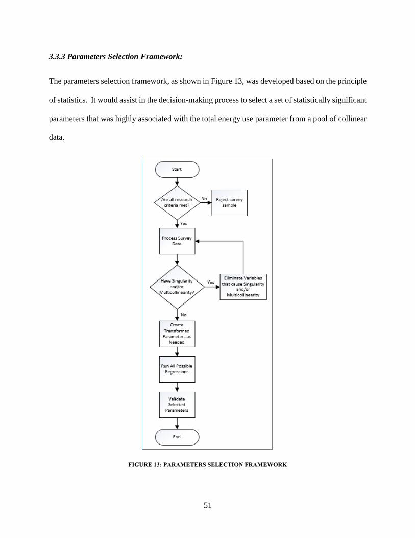
3.3.3 Parameters Selection Framework: ................................................................................................................................... 51
CHAPTER 4. RESULT AND DISCUSSION ........................................................................................................................... 54
4.1 THE SELECTION OF MODELS ............................................................................................................................................................... 54
4.2 DISCUSSION OF THE FINAL MODEL .................................................................................................................................................... 56
4.3 IMPROVE ENERGY EFFICIENCY IN THE WATER UTILITIES ............................................................................................................. 60
4.4 CHALLENGES AND LESSONS LEARNED ............................................................................................................................................... 61
4.5 A SCHEMATIC DIAGRAM OF THE IMPROVING CYCLE OF ENERGY BENCHMARKING ................................................................... 63
CHAPTER 5. CONCLUSION .................................................................................................................................................... 64
CHAPTER 6. FUTURE WORK ............................................................................................................................................... 65
6.1 WATERID – AN ONLINE DATABASE ................................................................................................................................................ 66
6.2 BENCHMARKING RATING SCORE ......................................................................................................................................................... 68
REFERENCES ............................................................................................................................................................................. 70
APPENDIX A: PARAMETERS OF WATER UTILITY SURVEYS DATA........................................................................ 75
Page 7
vii
LIST OF FIGURES
Figure 1: Proposed Framework to Eliminate Singularity and Multicollinearity .......................... 33
Figure 2: A Schematic Diagram of A Typical Drinking Water Utility ........................................ 34
Figure 3: Water Utility Samples Geographical Distribution ........................................................ 35
Figure 4: Total Energy Use Parameter.......................................................................................... 39
Figure 5: Ln [Total Energy Use] Parameter ................................................................................. 39
Figure 6: Elimination of Collinear Parameters Process ................................................................ 43
Figure 7: Singularity Diagnosis .................................................................................................... 45
Figure 8: Eliminations of Singularity ........................................................................................... 46
Figure 9: Multicollinearity Diagnosis 1st Iteration ....................................................................... 47
Figure 10: Multicollinearity Diagnosis 2nd Iteration ................................................................... 48
Figure 11: VIF Calculation ........................................................................................................... 49
Figure 12: Multicollinearity Analysis ........................................................................................... 50
Figure 13: Parameters Selection Framework ................................................................................ 51
Figure 14: Selection of the Transformed Parameters ................................................................... 52
Figure 15: Subsets of All Possible Regressions ............................................................................ 55
Figure 16: All Possible Regressions Result .................................................................................. 57
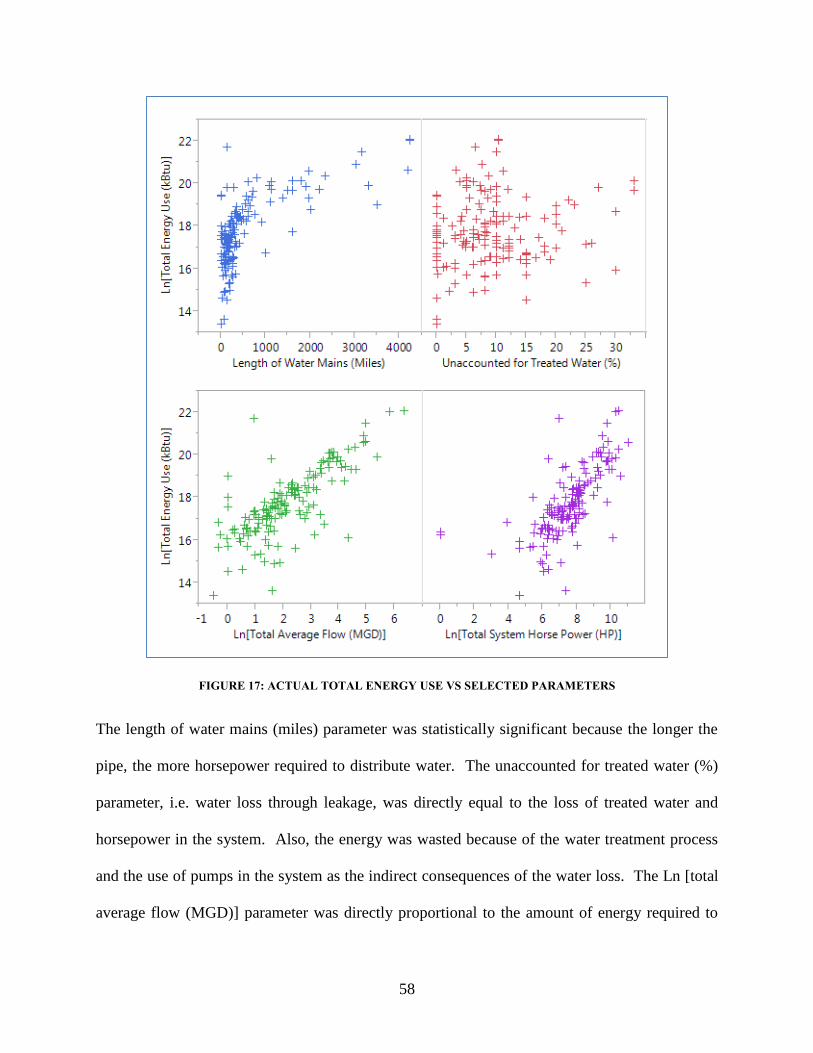
Figure 17: Actual Total Energy Use vs Selected Parameters ....................................................... 58
Figure 18: Relationships Between Four Energy Parameters and A Water Utility ....................... 59
Figure 19: Improving Cycle of Energy Benchmarking In Drinking Water Utilities .................... 63
Figure 20: The Data Extraction Process of WATERiD ................................................................ 66
Figure 21: WATERiD Benchmarking Example ........................................................................... 67
Page 8
viii
Figure 22: Distribution of Ln [Energy Use Ratio] ........................................................................ 69
Figure 23: Cumulative Probability Graph of Ln [Energy Use Ratio] ........................................... 69
Figure A1: Production Process ..................................................................................................... 75
Figure A2: Treatment Process ...................................................................................................... 77
Figure A3: Distribution Process ................................................................................................... 79
Figure A4: Overall Water Utility as a Whole ............................................................................... 80
Page 9
ix
LIST OF TABLES
Table 1: Existing Energy Benchmarking in Water Utilities ........................................................... 6
Table 2: Direct Energy Use Parameters ........................................................................................ 37
Table 3: Indirect Energy Use Parameters ..................................................................................... 41
Table 4: Individual Parameter Effect With Respect to the Total Energy Use .............................. 54
Table 5: Selected Models of All Possible Regression .................................................................. 56
Page 10
1
CHAPTER 1. INTRODUCTION
1.1 Water and Energy
Water and energy had been generally treated as two separate issues. However, water and energy
existences, known as water energy nexus, were closely related and mutually dependent resources
(NCSL 2009). With the current impact from the climate change, there was a need to thoroughly
understand the relationship between water and energy (Cabrera et al. 2010). The water
infrastructure demanded vast amount of energy, and energy production also required countless
volume of water. Therefore, a sustainable management of water would be largely depended on
energy and vice versa.
In the United States, there were more than 52,000 community water systems according to the U.S.
Environmental Protection Agency (U.S. EPA) (2007). In those 52,000 systems, only 4,000
systems had serving population over 10,000 people, and they accounted for approximately 85% of
the whole U.S. population. Water and wastewater utilities together consumed roughly 3% of total
U.S. electricity use. Many drinking water facilities throughout the nation had the energy costs as
the second highest, only second to the labor costs, of their annual operational budget according to
the U.S. EPA (2009).
There were many factors that affected the cost and amount of energy usage. Those factors were
associated with regulations, aging infrastructure, growth, treatment technology complexity, and
supply challenges (ISO 2005). In addition to its standard of high-priority concerns, the water
supply system also faced the increased health and environmental related regulatory requirements.
For example, the higher requirement of the drinking water standard mandated to have additional
Page 11
2
treatment such as the disinfection of microbial contamination (Liu et al. 2012). Such a treatment
required installations of high energy-intensive technologies.
Federal and States throughout the nation had searched for opportunities to reduce the energy
demand associated with the water supply system during peak hours. Ways to decrease the energy
use for operating water transportation and treatment systems were also in high demand.
1.2 Energy Efficiency in Water Utilities
Energy efficiency had been on agenda of most governments in the developed countries around the
world, especially for public policy and energy sustainability issues (Patterson 1996). The increases
in energy efficiency would promote industrial competitiveness, energy security, and
environmental surroundings.
Improving water efficiency was directly equivalent to improving energy savings because the less
energy would be used in the process such as pumps, thus it extended the service life of treatment
equipment and parts. Also, the financial savings resulted from fewer needs of chemicals and other
treatment materials (Leiby and Burke 2011). Thus, improving energy efficiency was a vital step
to reduce expenses for water utilities.
There were many opportunities that could help water utilities to reduce their energy consumption.
Implementing the energy efficiency practices would yield significant cost savings. Furthermore,
the activities such as optimizing current treatment, pumping, and operational practices could be
executed within a restricted budget.
At this moment, there were inadequate consideration on how to define and measure the energy
efficiency. Therefore, ways to evaluate how energy was being used over time can significantly
Page 12
3
improve not only energy management but also performance of the whole system (NYSERDA
2010). There were many tools that utilities could use to measure their total energy consumption
throughout the process of production, treatment, and distribution. The energy benchmarking was
one of the highly regarded approaches recommended by Water Research Foundation (2007).
The energy benchmarking could be an effective tool to compare the energy use of a utility with
the national average after normalized different utilities’ characteristics and operational functions.
The energy benchmarking result could be a good indicator that reflected the energy efficiency in
a water utility. In fact, the energy benchmarking could provide drinking water utilities measures
to improve their energy efficiency and serve as an initial step in the utility energy management.
1.3 Goal and Objectives
1.3.1 Goal
The goal of this research is to improve energy benchmarking practices in drinking water utilities.
It would help to improve existing practices on how to measure and select energy benchmarking
parameters. Therefore, the utilities can use those parameters to improve their energy efficiency.
The research scope covered the entire drinking water system including water transmission,
treatment, storage, and distribution.
1.3.2 Objectives
The study had three objectives as followings.
1. Identify the critical energy parameters to support the energy benchmarking
2. Develop the mathematical analysis to select energy parameters
Page 13
4
3. Recommend ways to improve the current benchmarking practices and create national
online database
Page 14
5
CHAPTER 2. LITERATURE AND PRACTICE REVIEWS
2.1 Energy Benchmarking in Drinking Water Utilities
The definition of benchmarking is “a continuous, systematic process for evaluating the products,
services, and work processes of organizations that are recognized as representing best practices for
the purpose of organizational improvement” (Spendolini 1992). In other words, benchmarking
was to compare performance metrics between one’s own organization with the best practices of
similar organizations in the industry, described by Water New Zealand (WaterNZ) (2012). Below
were the general benchmarking procedures:
1. Identify issues by metrics
2. Collect internal data to establish baseline
3. Compare data with peers
4. Analysis the system
5. Implement and monitor changes
Benchmarking in the water infrastructure system could not measure just the performance, which
most of all existing benchmarking focus on. The current performance benchmarking metrics, both
physical and functional, had no specific consideration of energy. There were, in fact, very limited
sets of standard for energy benchmarking in drinking water utilities.
From the literature and practice reviews of major water institutions worldwide, there were very
few water benchmarking that had energy parameters dedicatedly to measure the energy efficiency
in the water utilities. Out of the 16 benchmarking reports in the Table 1, there were only five that
had metrics specifically for evaluating energy performance.
Page 15
6
TABLE 1: EXISTING ENERGY BENCHMARKING IN WATER UTILITIES
Page 16
7
The current benchmarking practices are very lengthy with hundreds of parameters. Lots of existing
parameters had overlapped each other. They were time-consuming and complicated process.
Nonetheless, these benchmarking metrics could not reflect the actual energy efficiency of the
drinking water utilities. There were no direct correlations to be able to measure the system energy
performance effectively. Then, there was a need for better sets and meaningful standardized of
benchmarking parameters (Brueck et al. 2003) that were more concise and accurate, so the new
sets of benchmarking would reduce confusion and deliver maximum information within a timely
manner.
More importantly, the benchmarking results might serve as the initial baseline for all improving
efforts (WERF 2009). With compelling ideas from the results, the plant operators would be able
to identify areas where energy efficiency improvement should be executed and know how much
they could be improved. By comparing information of energy use with other utilities, energy
benchmarking was good for both encouraging improvement and sharing properly identified best
practices (Liu et al. 2012).
2.2 Potential Ways to Improve Energy Efficiency in the Drinking Water Utilities
2.2.1 Management Tools
The management tools could provide a better understanding of the current utilities’ energy
consumption and be used to define the intensive-energy-used area within the system. They could
set goals, define energy conservation measures, prepare implementation process, and monitor the
improvement (Leiby and Burke 2011).
Page 17
8
2.2.1.1 Benchmarking:
The designed metrics of energy benchmarking would help drinking water utilities to compare their
energy use. According to WaterRF (2011), the goals of benchmarking were to have performance
measurements in all areas of production, treatment, and distribution on energy related consumption
of the drinking water and utilities such as total flow, raw pumping horsepower, distribution
elevation change, etc. The data would be used to track changes and improvements internally and
to compare externally with other utilities in the industry.
Examples of benchmarking tools:
1. USEPA’s Energy Star Portfolio Manager
2. USEPA’s Energy Star Cash Flow Opportunity Calculator V 2.0.
2.2.1.2 Energy Audits:
The energy audit was one of the means that would allow the utilities to evaluate the whole system
and to locate sections and opportunities for energy efficiency improvement without having
negative impact system performance and water quality. Since the pumping of raw water to
distribution and treatment process accounted for roughly 80 percent of the energy use in the
drinking water plants, the plant operator would need to have energy audits to manage and assess
energy consumption of the utilities, a study by Leiby et al. (2011). The energy audits would spot
the most energy-intensive areas within the system and plan a series of potentials energy
conservation activities.
Generally, there are two types of energy audits. They are a “high-level” or a comprehensive
“detailed process.” A high-level or walk-through energy audit is typically performed to evaluate
Page 18
9
the most energy-use intensive component or other key problem areas of the system. It would
dictate when and where the detailed process energy audit should be performed. The detailed
process audit concentrated on the assessment of a certain area or operation identified by the high-
level audit. In doing so, it would offer a comprehensive understanding and possible improvement
regarding to that issue. Common focal points for executing a detailed process energy audit would
be raw water pumping, distribution system pumping, filtration, and treatment processes. An
energy inventory could be created from data gathered during the energy audit. Moreover, the
information from the energy audit and energy inventory would help the utilities staffs to develop
an energy map.
The processes of performing both high-level and detailed process audit were fairly similar, but the
difference was in the detail of data collection. The detailed process audit would concentrate on a
particular component or operation while the high-level audit focused on the overall system. Below
was an energy audit process outline as described in the Electric Power Research Institute (2011):
Holding a kickoff meeting
Creating a team of water utility staff, electric utility personnel, and outside experts
Collecting plant or specific operational process data, whichever is applicable for the type
of audit being performed
Evaluating electric bills and electric rate schedules
Conducting field investigations and holding discussions with operations staff
Creating an equipment inventory and distributions of demand and energy
Developing energy conservation measures and strategies
Following up on implemented measures
Page 19
10
Energy and Water Quality Management Systems:
The Energy and Water Quality Management Systems (EWQMS) was a model developed by Water
Research Foundation (WaterRF), Electric Power Research Institute (EPRI), and eleven of the
largest water utilities in the United States (WaterRF 2012). Even though EWQMS was a generic
model, it could be adjusted to suit a particular utility. With certain input information of a specific
utility, the EWQMS could provide a framework and execution plan to minimize energy costs while
still sustaining water demand and quality within the operational constraints and limited resources.
Thereby, the utility would have a specific plan stating how it should be functioned and what can
be anticipated, if operated accordingly.
The WQAMS was a sequence of separate application software application and operational
practices that could deliver flexible planning and scheduling maneuvers to resolve water quality
and energy management difficulties (Leiby and Burke 2011). In general, the operation of EWQMS
was accompanied by a utility Supervisory Control and Data Acquisition (SCADA) system. The
EWQMS would receive data from and give commands to a SCADA system to operate components
of a utility such as pumps and equipment at treatment facilities and distribution systems (WaterRF
2012). All in all, the benefits of EWQMS might include energy efficiency and water quality
improvement, cost savings, revenue increase, etc.
2.2.2 Plant improvements and management changes
To maximize the benefits of energy efficient improvement, drinking water and wastewater utilities
should implement improving measures on the whole process not just a particular
operation/treatment process. The typical facility-wide utility improvements involved lighting and
Page 20
11
heating, ventilation, and air conditioning (HVAC) upgrades for facility plant, ground, and building.
These improvements could be achieved easy and have no impact to the normal utility operations.
Also, installation of electric and natural gas submeters could give considerable savings to the
utility, yet the implementing expenses could be compensated if associated with installing new
utility equipment. The industrial trend was moving toward the use of an automatic control system
such as Supervisory Control and Data Acquisition (SCADA). Recommendation by WaterRF
(2011), the utility might apply for incentives and rebates to reduce the financial impacts from
electric providers and other government agencies like New York State Energy Research and
Development Authority.
Some challenges the water utility faced were related to the management changes that they had to
do with changing/modifying typical ways of decision makings to promote new policy or
procedural amendments. A water utility, and the local authority that owns the system, might have
to thoroughly prioritize measures of energy efficiency improvements. It also had to analyze where
and how to implement those measures considering its technical and financial competences. As a
result, the prioritization would allow the utility not only to reach its energy reduction goals but
also maximized its potential savings (Leiby and Burke 2011).
2.2.3 Water Treatment
Because of changing water quality regulations such as disinfection byproducts and micro-
biological inactivation as well as higher expectation of water quality from consumers, a water
utility had to adapt new treatment/disinfection technologies rather than using conventional
treatment. Those commonly founded treatment were coagulation, sedimentation, filtration with
choline disinfection. Generally, treating surface water systems accounted for 10 to 20 percent of
Page 21
12
the total energy costs according to WaterRF (2011), which the rest would be used for pumping
water from sources to the treatment plant and from plant to the end-users. Therefore, the biggest
potential energy savings would be in the distribution sector, yet many utilities saved significantly
in optimizing treatment.
The new standard on water quality would inevitably drive the water utility to acquire newer
technologies. For example, those new and energy-intensive technologies were reverse osmosis
and desalination. The utility might be able to solve energy problems by finding alternative
approaches. A drinking water plant, for instant, was located next to a river where it could adapt
riverbank filtration instead of using flocculation, sedimentation, and filtration processes but
disinfection (Leiby and Burke 2011).
It was very important for water utilities to be realistic and set achievable goals based on their
competencies; they had to carefully select treatment process/technologies that would be best for
the whole system optimization. Methods such as life cycles costs, payback, and overall benefits
of economics input-output life cycle assessment could help water utilities to evaluate each
improving option. Some implementations might result in considerably higher energy savings than
others. However, the whole system optimization approach could be accomplished with the right
combination between the technology and other energy improvements. It would yield overall
energy reductions that have greater savings compared to each individual implementation.
2.2.4 Water Distribution
In the USA, the water industry used roughly around 3% of total electricity production, and up to
90% of this 3% total electricity was consumed by pumps (Bunn and Reynolds 2009). Water was
Page 22
13
comparatively liquid. It weighted round 62.4 pounds per cubic feet or 8.34 pounds per US gallon.
The energy efficiency improvements in the water distribution system had two main approaches.
First was enhancing the efficiency of generating water pressure, and second was reducing in
amount of water pressure demand.
Optimization of the complete water distribution system including pipes, storage, valves, etc.—
which can lead to resize pump capacities and the total number of pumps accordingly—could
facilitate energy needs to pump water. A large capital investment was not always necessary to
implement the system efficiency improvements or total energy reductions, often it was not required
at all. A vital tool to evaluate energy efficiency improvements of the water distribution system
was life cycle cost analysis. In several incidents, a lesser-expensive capital investment option
might cost more if operated over the life of the equipment (Leiby and Burke 2011).
Our nature offered way to reduce energy use in the water distribution system that is gravity. The
gravitational potential energy could save pumping energy and be substituted for pump power such
as hydraulic flocculation. An ideal situation would be treating and delivering water at the water
sources where was considerably higher than the demand sites, thus gravitational potential energy
could be used for all transportation activities. However, this idea seemed to be far from realistic
because it was not financially feasible to reconstruct the entire water system and there were limited
water resources at high altitude. A more feasible alternative for the water utility would be to
manage the water pressure more effectively. Therefore, there was a need for pump optimization.
Page 23
14
2.2.4.1 Pump Optimization
Since most of the water utilities in the developed world had been using Supervisory Control And
Data Acquisition (SCADA) systems and operate telemetrically, they could use their historical
operational data stored in the database to assist in decision-making and performance improvement
(Bunn and Reynolds 2009). The small improvement in term of pump efficiency would result in
significant amount of energy saving and consequential drop in carbon emissions to the air.
Initially, a water utility had to make sure that pumps were performing close to the best efficiency
point (BEP). The optimization process was very complicated because it involved not only pumps
but also several associated pump components such as motor, valves, pipes, etc. The complete
understanding of water distribution system characteristics had to be attained before starting the
optimization. Activity such as resizing pumps, maintaining consistency, upgrading/rehabilitating
motors and others components, etc. were common measures to increase pumps’ efficiency.
Equipping variable speed or frequency drives to pump motors would increase their efficiency if
operating under the optimum output, particularly for low pump capacities. Replacements of old
pump motors with more efficient and more appropriate size pumps were advised if it becomes
more economical and engineering-sound improvements. The cumulative savings resulted from
increasing energy efficiency from a constant use of motors and pumps to a water utility can be
significant (Bunn and Reynolds 2009; Leiby and Burke 2011).
2.2.4.2 Pump Scheduling Optimization:
To optimize pump scheduling, first, the initial selection of a pump was important to match
operational requirements. Second, the maintenance and refurbishment in a timely manner needed
Page 24
15
to be well established to continue optimal performance. The last and most importantly process
was to dynamically optimize the scheduling of pump operation to improve efficiency. It could be
achieved by changing daytime and nighttime water demand patterns to best reflect the daily usage.
Moreover, practices of data-mining techniques and real-time dynamic optimizations could
considerably increase the energy efficiency to the system (Bunn and Reynolds 2009).
2.2.5 Water Conservation
The U.S. drinking water and wastewater utilities used as much as 56 billion kWh annually—
adequate to supply needs of more than 5 million homes for a whole year—that extensive amounts
of energy were in demand to treat and deliver water, reported by WaterRF (2011). In the drinking
water utilities, the energy would be used for raw water extraction and transportation, treatment,
storage, and distribution. Pumping of raw and clean drinking water accounted for a majority of
the total energy use. If drinking water utilities could reduce the amount of water being extracted,
treated, and distributed, they would save energy magnificently.
Several drinking water utilities and municipal authorities promoted water conservation plans and
programs to their industrial and residential sectors in order to decrease water demand (which in
turn would reduce the energy costs). Normally, the written water conservation document described
the evaluation of existing and future water use. It analyzed infrastructures, operations, and
management practices. The conservation plan assessed not only how to reduce the water use,
waste, and leakage but also described measures to improve the efficiency of the whole system from
treatment, store, and distribution processes (Leiby and Burke 2011).
Page 25
16
A holistic approach would help water conservation programs to manage both supply and demand
sites more effectively. It also determined alternative water resources for potable and non-potable
supplies. Basically, the supply-site focused on managed available water resources, maximized the
water utilities operational efficiency, and minimized water loss in the system. Even though
implementing the plans would need a substantial amount of financial investment, there were
potential revenues from water loss recovery and savings in operating costs. For demand-site
approach, the most important problem was a leakage, so implementations of the effective water
loss management strategies with conducting water loss audits were recommended by Leiby et al.
(2011). Results of the water audits would assist utilities to analyze the real loss of water in the
system. Then, they could initial programs like proactive leak detection, upgrade water meter
accuracy, recordkeeping, repair, and maintenance. The conservation planed for demand-site may
decrease revenues of drinking water utilities because of lower in water demand, but a more
reflective pricing rate could compensate those expected losses.
Water conservation plans might be varied due to the size of the water utilities and their uniqueness.
WaterRF guidelines (2011) for typical water conservation plans included following processes:
Establish the goals of the water conservation plan
Conduct a water system audit
Prepare a demand forecast
Identify and select potential water conservation measures
Page 26
17
2.2.6 Alternative/Renewable Energy Sources and Recovery Energy
Alternative/renewable energy meant energy generated from resources that could naturally
regenerate and be used in a sustainable way. Renewable energy projects in the drinking water and
wastewater utilities involved equipping with devices or system that could generate energy such as
heat and electricity and replacing the use of non-renewable/fossil fuel energy use by renewable
energy. It was notable to understand that the renewable energy project principle was to displace
the use of energy from fossil fuel with more green and sustainable energy supply. It did not intend
to decrease the amount of energy use like energy conservation measures. Therefore, the renewable
energy project might have a lengthy return on investments. Most renewable technologies’
performances relied on the environmental conditions such as wind, solar radiation, geothermal
power, etc. (Leiby and Burke 2011).
The U.S. Environmental Protection Agency (2008) encouraged all drinking water and waste
utilities to commit to explore and increase the use of alternative green energy technology rather
than the fossil fuel. The benefits of using renewable energy were not only to reduce the
environmental impacts but also to save operating costs for water utilities in a long term.
Examples of best practices for alternative/renewable energy sources were:
Solar Power: Concentrating Solar Power and Photovoltaic Solar Power
Wind Turbines
Geothermal
Lake/ocean Water Cooling
Micro-Hydro Generation
Page 27
18
Combined Heat and Power Systems
2.2.7 Financial Assistance
Essentially, implementations of the energy efficiency measures would require a considerable
amount of capital investment from water utilities. It was crucial for them to know that there were
lots of opportunities to apply for financial assistances for projects related reduction in energy
consumption and renewable energy use. Many Electric and gas providers provided financial
incentives. They, for instance, offered rebates and reduced energy rates for those utilities that
installed energy efficient equipment or implemented management practices to improve energy
efficiency. In some cases, water utility could take advantages of financing mechanism. It would
permit utilities to install energy conservation measures without paying a total amount at once—
those installing costs would be paid back out of guaranteed energy savings.
New York State Energy Research and Development Authority Programs and other States funding
organizations accommodated a wide range of financial assistances, incentives, and loans. They
could come in as shared-cost energy efficiency studies, loan funds to moderate costs of energy
efficient equipment, or incentives for renewable energy projects.
For Drinking Water and Clean Water State Revolving Funds (DWSRF and CWSRF), these funds
provided low-interest loans for utilities to use for projects such as energy efficiency and water
efficiency projects. Utilities might apply funds for installation of water meters, utility energy
audits, retrofits or upgrades to pumps or treatment processes, on-site production of clean water,
replacement or rehabilitation of pipe, etc.
Page 28
19
All in all, drinking water and wastewater utilities were highly encourage to explore available
financial assistances to help supporting their energy efficiency projects, and they might have to
use a combination of incentive programs and available funding resources to finance the project
(Leiby and Burke 2011).
2.2.8 Partnerships
Collaborating with partnerships would help water utilities to pursue many energy efficiency
opportunities available. There were two major types of partnerships which were public sector
partnerships and fee-supported industry partnerships. These partnerships would circulate
management best practices of implementing energy efficiency, share ways to improve energy
efficiency, and train water utility operators to enhance their competencies by experts (Leiby and
Burke 2011).
First, public sector partnerships usually consisted of federal government, state government, and
university. This kind of partnerships provided not only financial support but also information and
technical expertise. Public sector partnerships would inform water utilities about existing
management best practices and ways/ new technologies to improve system efficiency with no cost.
Also, the public sector partnerships would assist utilities to start improving and tracking their
energy efficiency measures.
The second type was fee-supported industry partnerships and trade groups that would connect
water utilities with a network of industry connections and knowledge for paid subscribers. These
trade associates and business networks would allow utilities to expose to other organizations in
addition to exchanges of knowledge, best practices, and energy efficiency innovations. Utilities
Page 29
20
would be benefited for their performance/energy audits and benchmarking by substantial data and
information of the industry.
2.3 Development of Energy Benchmarking
There are small numbers of benchmarking studies that considered measuring the energy efficiency.
Below were studies that discussed ways to develop benchmarking and to select parameters in order
to measure energy efficiency in the water utilities.
2.3.1 Towards the Improvement of the Efficiency in Water Resources and Energy Use in Water
Supply Systems:
Souza et al. (2010) proposed the methodology to analyze and improve the efficiency in water
resources as well as energy use in the water supply systems. The focuses were on water losses and
energy management. The studied discussed short, medium, and long term actions for three level
of planning including strategic, tactical, and operational. Performance indicators, simulation
models, optimization procedures, etc. were identified as decision support tools to address the water
loss issue and enhance the energy management in the water supply systems. The performance
indicators were rated only as good starting points by authors. They were unable to effectively
diagnose the energy use of the whole water system.
2.3.2 Management Evaluation of Water Users Associations Using Benchmarking Techniques:
Córcoles et al. (2010) stated that benchmarking was one of many important practices to improve
water and energy management. The goals of this study were first to systematically categorize
performance and energy indicators. Then, it would apply statistical method to reduce numbers of
those indicators. Authors used the Principal Components Analysis (PCA) and the Cluster Analysis
Page 30
21
(CA) as the combined application of multivariate techniques to evaluate and group indicators based
on their contributions. The study concluded on the most significant indicators that were easy to
get and deliver maximum information.
2.3.3 Energy Star:
U.S. EPA (2012) had developed a program called “Energy Star” to promote energy efficiency for
both businesses and individuals to help improving not only energy but also financial and
environmental performances for participants. The benchmarking scores were statistically
calculated and compared with the national average, gathering by U.S. Department of Energy’s
Energy Information Administration, using a regression analysis to select associated energy
parameters. The rating scores from 0 to 100 were proposed representing in percentile basis.
Although the mathematical approach in developing the energy benchmarking was useful, the EPA
had not had a specific benchmarking for the drinking water utilities.
2.3.4 Measuring Energy Efficiency in Urban Water Systems Using a Mechanistic Approach:
Gay and Sinha (2012) proposed the Thermodynamic Score to evaluate the performance of a utility
in comparison with its own potential maximum efficiency. A mechanistic approach could indicate
how effectively a water utility performed by compared with its system configuration. The
methodology for analysis was developed based on the minimum required energy. For example,
factors such as pump efficiency, wire-to-water efficiency, pressure, elevation, friction, head loss,
age, etc. were incorporated to find the minimum required energy for each utility. Therefore, this
study delivered the intuitive meaning and improved understanding of energy use with in the utility.
Page 31
22
2.3.5 Web-Based Benchmarking of Drinking Water Utilities in the United States:
This project was to develop the web-based benchmarking that would allow water utilities to
compare performance among peers by Rathor and Sinha (2013). Although there was lots of
performance benchmarking available in the industry, they focused on one or few areas of
performance. Each benchmarking measured in the similar fashion—which resulted in many
repeated indicators—if compared one to the others. Water utilities staff, furthermore, were not be
able to answer to some indicators because of differences in the physical characteristics.
Therefore, the authors consulted water utility personals and consultants to evaluate and finalize
sets of indicators that well represented the performance of the drinking water utilities. They
prioritized indicators that needed to be readily measurable, generic, and comparable. Accordingly,
the 57 essential indicators and 32 preferable indicators were chosen to use as the performance
benchmarking in the water utilities.
2.3.6 A Meta-Regression Analysis of Benchmarking Studies on Water Utilities Market
Structure:
Carvalho et al. (2012) conducted benchmarking studies of water utilities market structure. The
authors used a statistical method called “meta-regression analysis” to evaluate the impacts of scale
and scope economies in the water utilities. The meta-regression was used to investigate the
relationships between characteristics (explanatory variables) of samples from public studies with
respect to the scale economies and the scope economies (response variables). The study concluded
findings based on the statistical significances of each variables, and it used coefficient of the
regression model to interpret relationships among variables.
Page 32
23
2.3.7 Energy Index Development for Benchmarking Water and Wastewater Utilities:
The Water Research Foundation (WaterRF) (2007), former the American Water Works
Association Research Foundation (AwwaRF), took types of energy use, treatment characteristics,
services quality, etc. into account to develop energy benchmarking tool for water utilities with an
indexed score to make comparisons of energy use among water utilities in the nation. The
benchmarking tool was based on the same methodology of US EPA Energy Star for energy
efficiency of building using linear regression analysis.
The WaterRF study used a three-parameter regression model that it would judge by highest
significance by a t-test of a parameter with respect to the Ln [total energy use] parameter and the
total flow parameter. To be qualified for the next step, each parameter needed to have t-test value
higher than 2.0, equivalent to 0.05 p-value, to prove to be statistical significant. Six parameters
were selected by the industrial experts using the heuristic approach from the pool of 21
independent parameters. Finally, the study conducted the linear regression analysis on those six
parameters to fit a model with respect to the total energy use parameter. The WaterRF regression
model consisted of six parameters including: 1. Ln[total average flow (MGD)], 2. Ln[average
purchased water flow (MGD)], 3. Ln[difference between highest and lowest system elevation
(feet)], 4. Ln[source water pumping horsepower (hp)], 5. Ln[length of water mains (feet)], and 6.
Ln[total system horsepower (hp)]. The model yielded 0.87 R-Square value.
There were three major concerns about the WaterRF study:
1. The study did not consider relationships between each individual parameters as a whole
because it evaluated only three parameters at a time. Therefore, it did not examine the
Page 33
24
impact of a parameter that might cause other parameters to be either statistically significant
or insignificant if being analyzed all parameters at once.
2. Some of the final parameters were independently chosen based on the nature of the
characteristic rather than solely on statistical significance.
3. The study did not take the likelihood of singularity and multicollinearity problems into the
consideration. The singularity and multicollinearity problems originated from the collinear
data. The regression model should not have neither singularity nor multicollinearity
because they would make the regression model unable to accurately analyze the effects of
each individual variables.
2.4 Statistical Analyses
2.4.1 Regression
Regression analysis had arguably been the mostly widely used statistical technique for researchers
in all field including but not limited to engineering, science, management, economics, etc. (Awe
2013). It had many useful applications to describe, predict, and control relationships between
variables (Chatterjee et al. 2000). These applications were often overlapping, and their equations
might be valid for some or all of the mentioned purposes. The goal of each regression model
would dictate what criteria were needed to be considered in the developing phase, so the selected
variables to be in the regression model might be different. As a result, there was no the best set of
variables that could flawlessly serve for all purposes.
The purposes of using the regression analysis could be grouped into three main categories
(Chatterjee et al. 2000):
Page 34
25
2.4.1.1 Description and Model Building:
A regression equation could be used to describe the relationships between variables in the complex
interacting system. It could clarify complicated interactions of the given system. In doing so,
there were two major methodologies. First method was to have a large numbers of variables in
the regression model to account for all possible variations. Second was in the opposite direction
which was to have numbers of variables as small as possible for the sake of uncomplicated
interpretation and understanding of the regression model. This method chose a smallest set of
explanatory variables that could account for considerable parts of variation with respect to the
response variable.
2.4.1.2 Estimation and Prediction:
The regression model could be used for purposes of estimation and prediction. The regression
equation had the ability to predict the value or estimate the mean response of future observation
based on the given information. To build a regression model for these purposes, the main criteria
was to have minimum Mean Squared Error (MSE) of prediction while selecting explanatory
variables.
2.4.1.3 Control:
The regression model could be treated as a controlling tool. In this case, the regression equation
was set as a dependent function that has Y as the dependent variable. The independent/explanatory
variables were adjusted to match the particular result of the equation outcome. To use the
regression model as a controlling tool, the coefficients of independents variables must be precisely
calculated to keep the standard errors of the regression equation small.
Page 35
26
2.4.2 Variable Selection Process
In some regression problems, a set of variables were already selected beforehand to be included in
the analysis. Usually, the next step was to examine the equation to check the functional
specification or assumption about the error terms (Chatterjee et al. 2000). However, there were
other regression problems that had not yet determined what variables to be used in the regression
equation. Without theories or assumptions assisted in choosing variable, the variable selection
procedure was very important step to determine a set of variables for a regression model.
The variable selection procedure could help to select a set of variables from a very large numbers
of variables that could be potential predictors. It was the process that analyzes the relationships
between predictor variables on how they affected the response variable individually and mutually.
There were two ways to select variables in the regression model:
1. All possible regressions (Equation all)
2. Stepwise procedures
2.1. Forward selection
2.2. Backward elimination
2.3. Stepwise regression
2.4.3 All Possible Regressions
Principally, it was a regression type that would evaluate all possible linear regression models of a
given pool. The all possible regressions would try to fit all possible combinations of variables that
included the intercept of β0 and all numbers of regression variables. If there were 𝑥i , i = 1,2,3, …
, T variables, the all possible regressions would evaluate the total of 2T potential models (Golberg
Page 36
27
and Cho 2004). Since the all possible regressions would calculate all possible subsets of the pool
of variables, it would select the best model based on given criteria. The criteria could be as
following:
1. R-Square – quantity of the variation in the response from the least square fit
2. RMSE – Root Mean Square Error
3. Cp – Mallow’s Cp criterion
4. AICc – Corrected Akaike’s Information Criterion
5. BIC – Bayesian Information Criterion
In comparison with the Stepwise regression, the all possible regression had many advantages over
the Stepwise procedures (Golberg and Cho 2004). First, the three methodologies in the stepwise
procedures could not guarantee any type of optimality in the model. Second, three methodologies
of the Stepwise procedures did not essentially have the same set of regressors in their final model.
Third, the Stepwise procedures sometimes selected a set of regressors that were not “uniquely
superior” from a pool of independent variables. Lastly, all of these three methodologies would
provide only one final model; therefore, the researcher was forced to accept the model
unconditionally even though that model might or might not be the “best” regression model.
Regarding the variables selection process, Golberg and Cho (2004) stated that “The aim of
selection is always to maximize the ability to find out all of the ‘relevant’ information that is hidden
in the data.” Thus, all possible regression resulted to be a better option to find the “best” regression
model.
Page 37
28
2.4.4 Bayesian Information Criterion (BIC):
BIC calculates a model fit, and it was useful to compare between models (Golberg and Cho 2004),
as defined in Equation 1. The smaller number of BIC suggested a better fit. BIC was calculated
based on model fitness and complexity (number of variables). While the RSquare value tended to
increase with adding more variables to the model, BIC did not essentially change in that similar
pattern. It would, however, change with the combination of regressors to indicate the value of
fitness in the model. According to SAS Institute Inc. (2013), BIC could be termed as:
where
-2loglikelinood was computed by:
n * (ln (2 * pi ( ) *SSE/n) + 1)
k was the number of regressors
n was the number of observations
Although both BIC and AICc (corrected Akaike’s Information Criterion) were helpful measures
to compare fitness of models, BIC tended to select fitted models that had less parameters than
AICc (NCSS 2014). A set of selected explanatory variables based on smallest BIC were believed
to achieve both prediction capability (as many significant parameters as needed) and simplicity (as
minimum significant parameters as possible). Therefore, this study chose to use BIC as the model
selection criterion.
−2𝑙𝑜𝑔𝑙𝑖𝑘𝑒𝑙𝑖ℎ𝑜𝑜𝑑 + 𝑘ln(𝑛) EQUATION [1]
Page 38
29
2.5 Collinear Data
Collinear data could cause serious distortions if being analyzed by a standard procedure (Chatterjee
et al. 2000). If there were one or more small eigenvalues existing in the correlation matrix, it was
likely to have a collinearity problem. Essentially, there were two approaches to solve a
collinearity. First was to identify variables that cause collinearity, and sequential action was to
delete them to have a reduced dataset of noncollinear variables. The second method was to use a
tool called “ridge regression.” However, this method was not applicable to data set with a large
numbers of variables. Practically, the first method of deleting correlated variables was almost
always selected to compute variables selection with collinear data.
2.5.1 Singularity
In general, the simple linear regression model was formulated as in the Equation 2 (SAS 2013). If
the regression model had p parameters and n observations, the X became n x p matrix.
The regression coefficient 𝛽 could be found as shown in the Equation 3 below.
The coefficient, 𝛽, could be computed only if (𝑋𝑇𝑋) was nonsingular and invertible (Golberg and
Cho 2004; SAS 2013). However, in the case of singular matrices, the invert matrix of (𝑋𝑇𝑋) was
incomputable because there were linear dependencies between parameters. There would be at
least one parameter that it was a roughly linear combination of a group of remaining parameters.
𝑌 = 𝛽𝑋 + 𝜀 EQUATION [2]
EQUATION [3] 𝛽 = [(𝑋𝑇𝑋)-1][𝑋𝑇𝑌]
Page 39
30
2.5.2 Multicollinearity
The problems occurred when one or more independent variables (explanatory parameters) were
highly correlated with other independent variables. When independent variables were adequately
redundant, the impact of singularity and severe multicollinearity caused inability to accurately
distinguish effects of each variable.
The Variance Inflation Factors (VIF) and the correlation of parameter estimates could be used to
identify multicollinearity in the dataset.
2.5.3 Variance Inflation Factors (VIF)
VIF could indicate whether or not a specific variable had multicollinearity with respect to other
explanatory variables in the group and the response variable, as shown in Equation 4. VIF was
calculated from each of the explanatory variable in the model as a function of all other explanatory
variables. The VIF for the 𝑋𝑗 term could be defined as (SAS 2013):
where
p was the number of explanatory parameters in the regression model
𝑅𝑗2 was the coefficient of multiple determination, i.e. RSqure, for the regression of xj as a
function of the other explanatory parameters
If the 𝑋𝑗 had a strong linear relationship with other explanatory variables in the model, it would
make 𝑅𝑗2 value close to 1 and 𝑉𝐼𝐹j value large (Chatterjee et al. 2000). Golberg and Cho (2004)
𝑉𝐼𝐹j = 1
1−𝑅𝑗2 , j = 1,…,p EQUATION [4]
Page 40
31
wrote that if VIF value was greater than 10, it would suggest a possibility of having the
multicollinearity problem in the model. Consequently, multicollinearity might cause problems in
the estimating process.
2.5.4 Correlation of Parameter Estimates
The correlation of parameter estimates matrix is calculated to evaluate whether or not the
collinearity is present in the model (SAS 2013). The typical linear regression formula is defined
as:
where
𝛽0, 𝛽1, … , 𝛽𝑝 were the coefficients
𝑋1, 𝑋2, … , 𝑋𝑝 were explanatory variables
𝜀 was an error
In individual row of the data table, there were a value for response variable and values for the p
explanatory variables. The explanatory variables were considered unchanged in each observation,
while a response variable was considered as a function of a random variable. With fixed values of
explanatory variables for any set of response variables, the coefficient could be estimated. The
estimated coefficients could be different depended on the different set of response variables. The
correlation of parameter estimates, then, computed the theoretical correlation of the estimated
coefficients.
The correlation of parameter estimates calculated merely on an estimated of the interception and
values of the explanatory variables (SAS 2013). More importantly, the values of response
𝑌 = 𝛽0 + 𝛽1𝑋1+ . . . +𝛽𝑝𝑋𝑝 + 𝜀 EQUATION [5]
Page 41
32
variables had no effect on a correlation between a pair of two explanatory variables estimates.
Values of the correlation of parameter estimates were in a range of -1 and 1. The correlation value
at 1 indicated a direct relationship between a pair of explanatory variables in a perfect increasing
linear relationship, while the correlation value at -1 implied a direct relationship between a pair of
explanatory variables in a perfect decreasing linear relationship (Golberg and Cho 2004). If the
correlation value was at 0, it meant that the relationship between a pair of explanatory variables
was uncorrelated with little or no linear relationship.
2.5.5 Solving Multicollinearity
Multicollinearity problem could be solved. First, similar purposed variables were grouped
together. Multicollinearity diagnostic measures was run to identify variables that most likely to
have multicollinearity problem. The most widely used methodology to eliminate the collinear of
data was to delete a variable that had high VIF score (Chatterjee et al. 2000). If the VIF value was
higher than 10.0, it was likely that the variable would have multicollinearity (Golberg and Cho
2004). After detected collinearities, a group of variables that had VIF value over 10 would be
analyzed separately to explore relationships among them. The correlation of parameter estimates
investigatesd pairwise comparisons among the variables in the group. The high number would
indicate that a pair of variables is likely to have collinear relationship between them (SAS 2013).
With results from both VIF and the correlation of parameter estimates, a group of variables with a
collinear dataset was identified. The following step was to delete one variable from this group out
one at a time based on the least statistical significances (highest Prob>|t| value). The rest of the
available variables would check the VIF with respect to the response variable to find
Page 42
33
multicollinearity. The iteration would be repeated until none of variables in the pool have VIF
value greater than 10, thus it achieved the status of noncollinear dataset.
2.5.6 Collinearity Elimination Framework
Based on the discussed methodologies, the proposed framework is recommended to eliminate
collinear problems in the dataset as shown in the Figure 1. The framework starts with processing
dataset and then checks the singularity and multicollinearity among variables. It will repeat the
cycle of eliminating correlated variables until singularity and/or multicollinearity do not exist.
FIGURE 1: PROPOSED FRAMEWORK TO ELIMINATE SINGULARITY AND MULTICOLLINEARITY
Page 43
34
CHAPTER 3. METHODOLOGY
3.1 Data Collection
The study used the WaterRF (2007) survey da5a that was published with the Energy Index
Development for Benchmarking Water and Wastewater Utilities report. The WaterRF created this
survey to gather operating characteristic and energy use of the drinking water utilities. It was
developed based on templates of U.S. EPA ENERGY STAR benchmarking system for commercial
buildings, American Municipal Sewage Association (now the National Association of Clean Water
Agencies), EPA Community Water System, and Iowa surveys. The WaterRF sent out the water
utility survey instrument to 1,723 water utilities across the geographic distribution of the U.S. It
received the data back from 389 water utilities.
FIGURE 2: A SCHEMATIC DIAGRAM OF A TYPICAL DRINKING WATER UTILITY
In a typical drinking water utility, there would be three main processes according the WaterRF
(2007). They were production process, treatment process, and distribution process as shown in
the Figure 2 above. The parameters in this study consisted of 104 parameters measuring
throughout a water utility including water general parameters, raw water parameters, water
treatment objectives, water treatment processes and residual handling parameters, water
Page 44
35
distribution parameters, and water energy use parameters. All parameters were attached in the
Appendix A. The study had samples from 389 water utilities across the U.S. The geographical
distribution was displayed in Figure 3 below.
FIGURE 3: WATER UTILITY SAMPLES GEOGRAPHICAL DISTRIBUTION
Statistically speaking, terms of a “variable” and a “parameter” were used interchangeably in this
study. Essentially, a variable was any value, quantity, or characteristic of an observation. While
in the benchmarking term, a variable could be referred as a “parameter” that contained value of a
specific system characteristic. An observation was a survey result having information of
parameters from a water utility.
N = 389
Page 45
36
3.2 Observations
The process of this study started from the available 389 survey samples of water utilities. The first
decision-making point was to set research criteria. The research criteria mainly considered missing
value in each observation. First of all, the observation had to have the total energy use greater than
0 kBtu. Since this parameter was the only response parameter in this study, the regression could
not analyze energy related relationships from explanatory parameters without it. 188 observations
had either 0 kBtu or missing value. Also, it happened that 46 observations from New York utilities
had missing values in 13 quantitative parameters that measured horsepower, turbidities, well depth,
and elevations. Therefore, these 46 observations were excluded from the study as well.
The rest of the observations, then, had not been removed or modified to prevent bias and incorrect
relationships that may occur in the regression models. Therefore, the total numbers of available
observations were at 155 utilities.
3.3 Parameters
There were 104 parameters in each water utility observation. Out of these 104 parameters, 58
parameters were qualitative variables while 46 were quantitative variables. Most of the qualitative
parameters were nominal. Nominal parameters meant that values belonged to groups and the order
did not matter. Those were binary questions. Also, some of qualitative parameters were ordinal.
Ordinal values belonged to groups, and the order mattered. For example, the number of ground
water source was recorded by count, but the magnitude of the water source was not given.
Therefore, the decision was made to exclude those 58 qualitative parameters out of the total 104
parameters of this study. The relationships between the total energy use and those qualitative
Page 46
37
parameters were not meaningful to make any comparisons in this study. As a result, only 46
quantitative parameters (continuous variables) were included in the parameter selection process.
In the group of 46 quantitative parameters, parameters could be divided into categories. First was
a category of 16 direct energy use parameters to be used as response parameters, and the second
group was indirect energy use parameters that consisted of 30 explanatory parameters.
3.3.1 Response Parameter
The direct energy use parameters measured the amount of energy use in terms of electricity, natural
gas, fuel oil, and propane as well as their associated costs. The list of these 16 direct energy use
parameters, parameter #1-16, was shown in Table 2.
TABLE 2: DIRECT ENERGY USE PARAMETERS
All of these 16 direct energy use parameters were considered as response parameters. They would
be used to find relationships with other 30 indirect energy use parameters, which were the
parameter #1-30 in the Table 3.
Page 47
38
The singularity was found in the group of the total electricity use parameter in Equation 6. The
total electricity use parameter was the combination of production electricity use parameter,
treatment electricity use parameter, and distribution electricity use parameter. These parameters
became redundancies if they were included in the models (Golberg and Cho 2004). Therefore,
only the total electricity use was selected from this group.
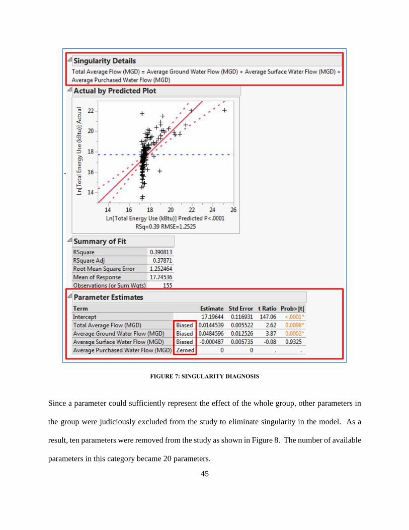
There was a need of a signal energy use parameter to represent the whole group of 16 direct energy
use parameters. First, the single parameter, the total energy use parameter (parameter #17), was
created to best capture effects of the entire group based on the annual average use of energy as
defined in Equation 7. This study used the source energy conversion factors according to the
WaterRF (2007) to convert electricity (parameter #1,4,7,10 in Equation 6), natural gas (parameter
#13), fuel oil and propane use (parameter #15) to be in a single unit of British thermal unit (Btu)
for the total energy use parameter.
These conversion factors were calculated based on the amount of energy in Btu to product a kWh
of electricity. It would take US national average of 11,100 Btu to generate a kWh of electricity
(DOE 2004). Fuel oil and propane were converted from a unit of sale volumes in gallon to kBtu.
In case of the natural gas, the conversion factor already took 2.4% transmission losses into an
account. The study used the natural logarithm to transform the total energy use parameter
Total Energy Use (kBtu) = [Total Electricity Use (kW) X 11.1 (kBtu/kWh)] +
[Natural Gas Use (Therm) X 102.4 (kBtu/Therm)] + [Fuel Oil (Gallon) X 141
(kBtu/Gallon)] + [Propane (Gallon) X 91 (kBtu/Gallon)] EQUATION [7]
Total Electricity Use (kWh) = Production Electricity Use (kWh) + Treatment
Electricity Use (kWh) + Distribution Electricity Use (kWh)
EQUATION [6]
Page 48
39
(parameter #17) in Figure 4 to be Ln [total energy use] parameter (parameter #18), so it would
have a normal distribution instead of skewed distribution as shown in Figure 5.
A set of energy cost parameters (parameter #3,6,9,12,14,16) and a set of peak energy use
parameters (parameter #2,5,8,11) were highly correlated with a set of energy parameter use
FIGURE 5: LN [TOTAL ENERGY USE] PARAMETER
FIGURE 4: TOTAL ENERGY USE PARAMETER
Page 49
40
parameters (parameter #1,4,7,10). As the test discovered multicollinearity among them, they were
statistically redundant with the Ln [total energy use] parameter. The Ln [total energy use
parameter was also compared with the original 16 parameters to find the relationships among them
to see if this parameter can be the best candidate for the group of 16 parameters. The founding of
singularity and multicollinearity indicated that these 17 parameters are collinear dataset, when
having the Ln [total energy use] parameter as a response variable and other 16 parameters as
independent variables. Results suggested that having only one response parameter (parameter
#18) was recommended to avoid problem of this collinear dataset.
All in all, the study selected the Ln [total energy use] parameter (parameter#18) to represent as the
only response variable of this study.
Page 50
41
3.3.2 Explanatory Parameters
In this group, there were 30 indirect energy use parameters (parameter #1-30 in table 3) that could
be used to explain the relationship with the response parameter.
TABLE 3: INDIRECT ENERGY USE PARAMETERS
The interpretation of multiple linear regression could be made if the assumption was true that the
explanatory parameters were not strongly correlated (Chatterjee et al. 2000). If the singularity
and/or multicollinearity existed in the dataset, the estimated effects of each parameter in the linear
regression were unreliable. For that reason, the interpretation of this study might not be valid
because there were strong linear relationships between these 30 indirect energy use parameters.
Page 51
42
The study used the statistical approach that was discussed earlier in the collinear data section of
chapter #2 to eliminate both singularity and multicollinearity problems in this dataset. The Figure
6 showed three-step process to address the collinear dataset. The first step was to eliminate the
singularity; there were 10 parameters with identified singularity out of a pool of 30 explanatory
parameters. The second and third steps were to exclude parameters that had multicollinearity out
of the dataset. Two parameters of the second step and three parameters of the third step were
classified with multicollinearity. The total of 15 explanatory parameters were available for the
parameter selection process.
Page 52
43
FIGURE 6: ELIMINATION OF COLLINEAR PARAMETERS PROCESS
Page 53
44
3.3.2.1 Singularity
The following groups of parameters had singularity problems among themselves. They were
groups of total average flow parameter (parameter #1,4,7,26 in Equation 8), total system
horsepower parameter (parameter #9,20,25,30 in Equation 9), average raw turbidity parameter
(parameter #10,12,27 in Equation 10), and difference between highest and lowest system elevation
parameters (parameter #18,19,29 in Equation 11).
The study used the JMP program from SAS to identify singularity in the dataset. The group of
parameters that shared the same unit were analyzed to check the singularity. In Figure 7, four
parameters of the Equation 8 were checked as explanatory parameters with respect to the response
parameter. As the result, the study found singularity detials that the total averge flow parameter
had direct relationship with the sum of average groud water flow, average surface water flow, and
avearge purchase water flow.
Total Average Flow (MGD) = Average Ground Water Flow (MGD) + Average
Surface Water Flow (MGD) + Average Purchased Water Flow (MGD) EQUATION [8]
Total System Horsepower (HP) = Source Water Pumping Horsepower (HP) +
Distribution Pumping Horsepower (HP) + Engine Driven Pump Horsepower (HP) EQUATION [9]
Average Raw Turbidity (NTU) = [Average Ground Turbidity (NTU) + Average
Surface Turbidity (NTU)] / 2 EQUATION [10]
Difference between Highest and Lowest System Elevation (FT) = High
Elevation (FT) - Low Elevation (FT) EQUATION [11]
Page 54
45
FIGURE 7: SINGULARITY DIAGNOSIS
Since a parameter could sufficiently represent the effect of the whole group, other parameters in
the group were judiciously excluded from the study to eliminate singularity in the model. As a
result, ten parameters were removed from the study as shown in Figure 8. The number of available
parameters in this category became 20 parameters.
Page 55
46
FIGURE 8: ELIMINATIONS OF SINGULARITY
Average Ground Water Flow (MGD) Removed
Average Surface Water Flow (MGD) Removed
Average Purchased Water Flow (MGD) Removed
Total Average Flow (MGD)
Source Water Pumping Horse Power (HP) Removed
Distribution Pumping Horse Power (HP) Removed
Engine Driven Pump Horse Power (HP) Removed
Total System Horse Power (HP)
Average Ground Turbidity (NTU) Removed
Average Surface Turbidity (NTU) Removed
Average Raw Turbidity (NTU)
High Elevation (FT) Removed
Low Elevation (FT) Removed
Difference between highest and lowest system elevation (FT)
Singularity #1
Singularity #2
Singularity #3
Singularity #4
Page 56
47
3.3.2.2 Multicollinearity
The next step was to exclude parameters with multicollinearity problem from a pool of 20
explanatory parameters. Having multicollinearity in the model, the regression would inaccurately
select parameters into a model because it was unable to analyze effects of each individual
parameters.
FIGURE 9: MULTICOLLINEARITY DIAGNOSIS 1ST ITERATION
The parameters were grouped together based on similarity of measuring characteristics. In Figure
9, the first iteration was based on the four different groups of WaterRF classification (2007). The
second iteration was all remaining parameters after the first iteration as shown in Figure 10.
Design Ground Water Flow (MGD)
Maximum Ground Water Flow (MGD)
Design Surface Water Flow (MGD) Removed
Maximum Surface Water Flow (MGD)
Average Well Depth (FT)
Peak Ground Turbidity (NTU)
Peak Surface Turbidity (NTU) Removed
Peak raw turbidity (NTU)
Total Average Flow (MGD)
Average raw turbidity (NTU)
Water Residual
Handling ParameterTotal Average Daily Residuals (LB/DAY)
Population of Service Area (People)
Size of Service Area (SQM)
Length of Water Mains (Miles)
Total Storage Volume (MG)
Average Distribution Pressure (PSI)
Unaccounted for Treated Water (%)
Difference between highest and lowest system elevation (FT)
Total Building Area (SQFT)
Total System Horse Power (HP)
Water General
Parameter
Raw Water
Parameters
Water Distribution
Parameters
Page 57
48
FIGURE 10: MULTICOLLINEARITY DIAGNOSIS 2ND ITERATION
Analyzing the multicollinearity used Variance Inflation Factors (VIF) to discover parameters with
the problems. If the VIF value was higher than 10.0, it was suggested that the parameter had the
multicollinearity (Golberg and Cho 2004). In Figure 11, the discovering process highlighted four
parameters that had VIF values higher than 10.0.
Design Ground Water Flow (MGD)
Maximum Ground Water Flow (MGD)
Maximum Surface Water Flow (MGD) Removed
Average Well Depth (FT)
Peak Ground Turbidity (NTU)
Total Average Daily Residuals (LB/DAY)
Population of Service Area (People) Removed
Size of Service Area (SQM)
Length of Water Mains (Miles)
Total Storage Volume (MG)
Average Distribution Pressure (PSI)
Unaccounted for Treated Water (%)
Total Building Area (SQFT) Removed
Total Average Flow (MGD)
Average raw turbidity (NTU)
Peak raw turbidity (NTU)
Difference between highest and lowest system elevation (FT)
Total System Horse Power (HP)
All Available
Parameters
Page 58
49
FIGURE 11: VIF CALCULATION
The next step was to see the relationships between those four parameters through the Correlation
of Parameter Estimates as shown in Figure 11. The values were in the range between -1 to 1. The
positive value recommended that a pair of parameters were highly correlated with the positive
slope, while the values negative suggested that a pair of parameters were highly correlated with
the negative slope. The zero value meant that a pair of parameter had no relationship between
them. More information was discussed in the section 2.4.4. In Figure 12, the high values of
correlated pairs of parameters both positive and negative were highlighted in red. The population
of service area parameter was highly correlated with the total average daily residuals, length of
water mains, and total building area parameters. The total building area parameter was excluded
from the study because it had the highest Prob>|t| (smallest t Ratio) values among parameters with
multicollinearity in Figure 11. The parameter with the multicollinearity would be exclude out one
at a time until the dataset became non-collinear.
Page 59
50
FIGURE 12: MULTICOLLINEARITY ANALYSIS
After two iteration of multicollinearity diagnosis, five parameters were subsequently removed
because of having multicollinearity problems. In fact, each of those five parameters had VIF value
greater than 10. These parameters were 1.) Design surface water flow, 2.) Peak surface turbidity,
3.) Maximum surface water flow, 4.) Population of service area, and 5.) Total building area. There
were only 15 remaining explanatory parameters in the pool.
Page 60
51
3.3.3 Parameters Selection Framework:
The parameters selection framework, as shown in Figure 13, was developed based on the principle
of statistics. It would assist in the decision-making process to select a set of statistically significant
parameters that was highly associated with the total energy use parameter from a pool of collinear
data.
FIGURE 13: PARAMETERS SELECTION FRAMEWORK
Page 61
52
This framework would scrutinize and recommend appropriate actions for issues such as the
qualitative parameters, missing values in observations, singularity, and multicollinearity within the
dataset. The following step was to analyze pairwise relationships between each explanatory
parameter and the response parameter. If a relationship of a pair was not a straight-line
relationship, the transformed parameter of the original explanatory parameter was created as an
additional parameter. For instance, the transformation could be in forms of a log scale or
polynomial to any degrees that would yield the highest R-Square value. Below are the criteria:
1. Analyzed the pairwise comparisons between the Ln [total energy use] parameter and each
of the 15 explanatory parameters
2. Created a transformed parameters if other forms of the 15 explanatory parameters had
better R-Square values
3. All original 15 explanatory parameters remained for the analysis
FIGURE 14: SELECTION OF THE TRANSFORMED PARAMETERS
In Figure 14, the total system horse power parameter was compared with the Ln [total system horse
power] parameter, (total system horse power parameter)2, and (total system horse power
Page 62
53
parameter)3 to find the best R-Square values. The Ln [total system horse power] parameter had
the best R-Square value, so it was kept for the next analysis. If the original form of parameter had
the best R-Square value, no additional transformed parameter would be needed.
As a result, the total number of explanatory parameters became 24 parameters that would be used
for the all possible regressions analysis. The 15 parameters were in their original forms, while 9
parameters were transformed using a natural logarithm. The list of 9 transformed parameters
included:
1. Design Ground Water Flow (MGD)
2. Maximum Ground Water Flow (MGD)
3. Total Average Daily Residuals (LB/DAY)
4. Size of Service Area (SQM)
5. Length of Water Mains (Miles)
6. Total Storage Volume (MG)
7. Total Average Flow (MGD)
8. Peak raw turbidity (NTU)
9. Total System Horse Power (HP)
The set of these 24 parameters were noncollinear, so they were ready to be selected through all
possible regressions based on the lowest BIC value.
Page 63
54
CHAPTER 4. RESULT AND DISCUSSION
4.1 The Selection of Models
Results of all possible regressions ranked effects of each individual parameter by R-Square value.
In Table 4, there were 15 explanatory parameters in their original forms and additional 9
transformed parameters. The Ln [total average flow] parameter had the highest R-Square value at
0.552 following by the Ln [total system horsepower] parameter at 0.462 and the length of water
main parameter at 0.440 respectively.
TABLE 4: INDIVIDUAL PARAMETER EFFECT WITH RESPECT TO THE TOTAL ENERGY USE
If there were 24 independent parameters, selecting all possible subsets to fit a model ranging from
1 parameter at a time to 24 parameters at a time would result to be 16,777,216 possible models.
All possible regressions calculated the RSquare, RMSE (Root Mean Square Error), AICc, and BIC
for all 16,777,216 possible models. The total of 231 models were plotted in the Figure 15. Those
Page 64
55
were models that had up to 10 lowest RMSE for each incremental number of parameters from 1-
24 terms.
RMSE was the square root of the Mean Square for Error that measured the standard deviation of
the random error (SAS 2013). The small the number of RSME, the better fit of the model would
be. However, RMSE was typically decreased with adding more terms to a model. The interest of
simplicity was usually one of the major factors for choosing the regression model along with
goodness of fit according to Golberg et al. (2004). The BIC was calculated based on both model
fit and complexity of the model, please see Equation 1. Therefore, the BIC was suggested to use
as indexes in this study to compare fitness among models (SAS 2013).
The three models in Table 5 had the smallest BIC value among all possible subsets. The first
model had 4 parameters with 436.66 BIC. The second and third models had three and five
parameters respectively with slightly larger BIC values than the first model at 437.74 and 439.11
respectively.
FIGURE 15: SUBSETS OF ALL POSSIBLE REGRESSIONS
Page 65
56
TABLE 5: SELECTED MODELS OF ALL POSSIBLE REGRESSION
4.2 Discussion of the Final Model
The model #1 in the Table 5 was selected to be the final model of this study. In Figure 16, the
value of Prob > F in the analysis of variance was small enough to indicate a very convincing
significance that these four parameters were statistically significant in the regression model.
Statically speaking, the set of these four parameters was highly associated with the Ln [total energy
use] parameter and had no singularity and multicollinearity. The adjusted R-Square value of the
model was at 0.663. These four parameters were 1. length of water main (miles), 2. unaccounted
for treated water (%), 3. Ln [total average flow (MGD)], and 4. Ln [total system horsepower (HP)].
The detail of all possible regressions result was presented in Figure 16. The Figure 17 showed
relationships between four parameters and the Ln [total energy use] parameter.
Page 66
57
FIGURE 16: ALL POSSIBLE REGRESSIONS RESULT
Page 67
58
FIGURE 17: ACTUAL TOTAL ENERGY USE VS SELECTED PARAMETERS
The length of water mains (miles) parameter was statistically significant because the longer the
pipe, the more horsepower required to distribute water. The unaccounted for treated water (%)
parameter, i.e. water loss through leakage, was directly equal to the loss of treated water and
horsepower in the system. Also, the energy was wasted because of the water treatment process
and the use of pumps in the system as the indirect consequences of the water loss. The Ln [total
average flow (MGD)] parameter was directly proportional to the amount of energy required to
Page 68
59
treat and transport water. This meant that the higher the total average flow, the higher the energy
demanded to treat water. The reason that Ln [total system power (hp)] parameter was considered
to be highly related with total energy use because the system horsepower was use to maneuver
water throughout the system. Furthermore, factors like high fiction loss, static pressure, leakage,
etc. would result in larger pump motor horsepower required.
Figure 18 showed the areas that each of the four parameters could be used to measure the energy
use in the water utility. In fact, this water utility model was production-oriented model. It was
used in this study in order to correspond with the structure of the WaterRF survey data.
FIGURE 18: RELATIONSHIPS BETWEEN FOUR ENERGY PARAMETERS AND A WATER UTILITY
All in all, the all possible regressions gave the flexibility to select models with compromise
between model fit and simplicity. In the future, the methodology would provide water utilities
options to select the model based on cost-effective analysis. For example, some parameters are
more economical and easier to collect the data than other parameters. Therefore, it may be more
Page 69
60
practical to choose some model over the others with a compromise on slightly lower accuracy of
prediction capability.
4.3 Improve Energy Efficiency in the Water Utilities
While consumers mostly dictate the amounts of total flow and water main length, areas of total
system horsepower (pumps) and water loss can be improved significantly. Followings are some
examples on how to improve energy efficiency for these two parameters. Leiby and Burke (2011)
recommended to improve the total system horsepower by installing new pumps that are better
fitting sized and more efficient. Also, the practices such as real-time dynamic optimization
technologies and data-mining techniques could be implemented to increase the energy efficiency
(Bunn and Reynolds 2009) along with Energy and Water Quality Management System (EWQMS)
(Jentgen et al. 2007). Increasing in the energy efficiency even by small percentages can lead to
substantial savings for consistently used motors and pumps over a period of time.
The unaccounted for treated water parameter measures is the water loss in the system.
Implementing leak assessment methodology can help to recognize leakage in the system (Lansey
et al.). Leak detection technologies such as infrared thermography, random/regular sounding
survey, acoustic, etc. can help to locate leaks. Reducing leakage would reduce both loss of treated
water and amount of energy used to treat water. It also improves the public health protection and
reliability of the water supply systems (Fanner et al. 2007).
Page 70
61
4.4 Challenges and Lessons Learned
The author realized through conducting this study that there were many possibilities to improve
the energy benchmarking in drinking water utilities.
1. The qualitative parameters should be avoided in the survey. The survey had 58 out of 104
parameters as qualitative parameters, i.e. binary variables with yes and no questions. These
qualitative parameters could not provide any good indications on how the energy was being
used in the system. For example, if a utility stated that it used a slow sand filtration process,
there was no amount of energy provided to make comparisons with other utilities in the
nation.
2. The ordinal number type parameters (values belong to groups, and the order matters) in the
survey needed to be normalized. Those parameters were given numbers that were simply
labels. They had no real quantitative value. For instance, the total number of pumps
parameter was incomparable without knowing the sizes of those pumps. The pump size
could be an enormous one at 5,000 hp or a very tiny one at 10 hp, but each individual pump
was counted as one pump. It did not take magnitudes into the consideration.
To normalize these ordinal parameters, the survey should create new parameters to improve
comparing capability. For example, the new parameters should be created in a series of
amounts according to flow rate range, pressure range, or horsepower range instead of the
total number of pumps parameter.
3. Incorporating the condition assessment parameters into the benchmarking was needed to
compare the current state of the system. The designed pump horsepower might not reflect
the real operational routine if the pump only was run constantly at its 70 percent efficiency.
Page 71
62
4. To improve accuracy of the energy benchmarking, the survey samples ought to be grouped
together utilities with similar characteristics such as the quality of raw water, system
topography, or specifically environmental and financial regulation. Then, the energy
benchmarking should be conducted among utilities within the same class.
It was not meaningful to compare the utilities in different places just based on a simple
parameter such as their energy use per unit cost. The study of Leiby and Burke (2011)
showed that an average retail price for electricity in New York was about 40 to 60 percent
higher than the rest of the US. The New York water and wastewater section, therefore, had
to spend approximately 35 percent more than the national average per unit basis even
though its utilities had roughly 10 percent more efficient than in the other states.
5. The survey data was not nationally distributed. Although the surveys were sent out to all
50 states, there were 9 states with zero response. The total of 26 states had two or fewer
responses. It was desired to have richer data to develop a genuinely national energy
benchmarking.
6. All missing value should be reported as missing/blank value not zero. It was possible that
some recorded zero value in observations might be missing/unreported values. Those zero
values found in the dataset might not be truly zero but placeholders for missing values.
Therefore, those zero values should not be treated as missing values and vice versa because
their effects were significantly different.
7. The dataset had relatively small numbers of useful observations. Some of the parameters
had extremely small variation, but others were highly different. Thus, the decision to
remove parameters out of the model because of the multicollinearity had to be made on
Page 72
63
very sensitive information. The results would possibly change if adding just a few more
observations. Therefore, there was a need for larger and good quality dataset.
4.5 A Schematic Diagram of the Improving Cycle of Energy Benchmarking
The cycle in Figure 19 is recommended by the author to improve the energy benchmarking. The
figure is a schematic diagram of the improving cycle of energy benchmarking in drinking water
utilities. This study was in the study to improve the current practice phase that would help to
improve energy benchmarking. There still is a need to have better defined parameters to capture
characteristics of the water utilities in a more effective way as in the improvement phase.
Therefore, researchers could have the improved energy benchmarking to collect new data to
upload in the national online database. The national online database was discussed in the future
work section. Consequently, this cycle would improve the performance of the future energy
benchmarking in both reliability and accuracy.
FIGURE 19: IMPROVING CYCLE OF ENERGY BENCHMARKING IN DRINKING WATER UTILITIES
Page 73
64
CHAPTER 5. CONCLUSION
It was important to know how individual plan configuration, load, and operational factors could
be linked and affect to the energy use of water utilities. In doing so, energy benchmarking could
be a very useful tool to measure how energy is being used in the systems. It was also a crucial
step to improve the energy performance of the drinking water utilities. Having energy
benchmarking, the utilities could use those parameters to improve their energy efficiency.
The goal of this study was to use a quantitative approach to select energy benchmarking parameters
for the drinking water utility. It would use a mathematically objective method rather than heuristic
assumptions and/or subjective approach from the industrial experts.
The study used the national survey data of the drinking water utilities collected by the WaterRF.
Although the WaterRF survey was collinear dataset, those parameters with singularity and/or
multicollinearity were statistically examined and excluded from the dataset. The study applied the
variables selection method, called “all possible regressions,” to select a subset of parameters from
available independent/explanatory parameters in noncollinear dataset. Significant parameters that
were statistically selected based on their statistical significance. As a result, the all possible
regressions provided list of models that each had different subsets of explanatory parameters. In
each model, individual parameters were considered as highly associated with the total energy use
parameter. The model was selected based on the lowest BIC value. The regression model was
believed to have a good predictive capability to estimate the total energy use of a water utility.
It was suggested by the author that following steps of the improving cycle should be taken to arrive
the desired energy benchmarking in drinking water utilities: energy benchmarking; collect new
data; national online database; study to improve the current practice; and improvement phase.
Page 74
65
CHAPTER 6. FUTURE WORK
The future work is to develop a good survey instrument with better-defined parameters. It was
clear that the data collecting protocol ought to be improved. It is needed to concentrate on energy
related parameters and avoid qualitative parameters. All parameters should be normalized and
incorporate current condition assessment. To get a better perception of energy efficiency in water
utilities, the energy benchmarking should benchmark among utilities that have similar system
characteristics to avoid high benchmarking outcome variation, if comparing against utilities with
totally different system operational features.
The integration of existing technologies will improve the reliability and accuracy of data.
Implementation of sensors is recommended not only to eliminate human errors but also to improve
the data recording frequency. Also, the internet can improve communication paths to get data
from water utilities faster instead of a current practice that is heavily relied on the postal mail
service. The ultimate goal is to have real-time data of all participated water utilities available in
online database. The last step would be to develop algorithms to do real-time analysis and update
benchmarking results online accessible for user interface through a standard website or an
application of a mobile device.
The author would like to discuss two practical features of the energy benchmarking, WATERiD
and the benchmarking rating score. They can be improve substantially with better defined energy
benchmarking and richer dataset.
Page 75
66
6.1 WATERiD – An Online Database
WATERiD is the water infrastructure database that shares useful information online through web
interface. The online benchmarking has been developed for water utilities on this database, but
there is no specially energy benchmarking yet. The process of getting the data started from survey
files are sent to a water utility electronically. The files are in standard forms asking to fill out
values of parameters. The water utility will be asked to save those files in the File Transfer
Protocol (FTP). Next, the Extract, Transform, and Load (ETL) program is used to deliver the data
from the files located in the FTP and then display them on the WATERiD. The data extraction
process in Figure 20 is programed to be automated. The example of the benchmarking result is
displayed in the Figure 21. The benchmarking data could be made publically accessible. The
online database and web interface could improve the collecting data process because it makes the
process easier and quicker to communicate between researchers, water utilities, and consumers.
FIGURE 20: THE DATA EXTRACTION PROCESS OF WATERID
Page 76
67
FIGURE 21: WATERID BENCHMARKING EXAMPLE
Page 77
68
6.2 Benchmarking Rating Score
The benchmarking rating score is developed to help water utilities to compare themselves with
peers in the industry. After having a better defined survey instrument, a new dataset will be
collected from water utilities with similar characteristics. The dataset will use the parameter
selection framework and all possible regressions to select a set of significant parameters with
respect to the total energy use. The final regression model is chosen, so that the regression equation
can be formulated. The regression model will be able to predict the energy use of a water utility.
The energy use ratio is defined in Equation 12. A water utility will be asked the actual energy use
along with values of significant parameters of the final regression model. The values of significant
parameters will be used to calculate the predicted energy use in the regression equation.
In Figure 22, the Ln [energy ratio] values were graphed to see the distribution. The ratio of 1
means that the actual energy use is equal to the predicted energy use. If the ratio is lesser than 1,
it indicates that a water utility consumes energy less than the predicted value. If the ratio is greater
than 1, it implies that a utility use energy more than the predicted value. It is crucial to know that
the following examples are shown solely for the conceptual purposes. The actual results may be
different from these examples.
𝐸𝑛𝑒𝑟𝑔𝑦 𝑈𝑠𝑒 𝑅𝑎𝑡𝑖𝑜 = 𝐴𝑐𝑡𝑢𝑎𝑙 𝐸𝑛𝑒𝑟𝑔𝑦 𝑈𝑠𝑒
𝑃𝑟𝑒𝑑𝑖𝑐𝑡𝑒𝑑 𝐸𝑛𝑒𝑟𝑔𝑦 𝑈𝑠𝑒 EQUATION [12]
Page 78
69
FIGURE 22: DISTRIBUTION OF LN [ENERGY USE RATIO]
To compare the energy use ratio of a water utility with other utilities in the industry, the cumulative
probability graph of Ln [energy use ratio] is created from energy use ratio of all utilities, as shown
in Figure 23. For example, if a water utility has an energy use ratio at 0. 95, the energy performance
score of that water utility would be ranked at the 85 percentile (1.0 - 0.15 = 0.85) among peers in
the water industry.
FIGURE 23: CUMULATIVE PROBABILITY GRAPH OF LN [ENERGY USE RATIO]
Good
Bad Good Good Bad
Page 79
70
REFERENCES
Awe, O. (2013). "Regression Methods." Virginia Tech, Virginia Tech Laboratory for
Interdisciplinary Statistical Analysis.
BEE (2008). "INDIA Manual for the Development of Municipal Energy Efficiency Projects."
Bureau of Energy Efficiency, India.
Berg, C. v. d., and Danilenko, A. (2011). "The IBNET Water Supply and Sanitation Performance
Blue Book The International Benchmarking Network for Water and Sanitation Utilities
Databook." The International Bank for Reconstruction and Development / The World
Bank, Washington, DC.
Bow, S., Betham, E., and (PWWA), T. P. W. a. W. A. (2011). "Development of a Water Utility
Benchmarking System." Pacific Water and Wastes Asscociation.
Brueck, T., Riddle, R., and Paralez, L. (2003). "Consortium Benchmarking Methodology Guide."
Awwa Research Foundation and American Water Works Association.
Bunn, S. M., and Reynolds, L. (2009). "The energy-efficiency benefits of pumpscheduling
optimization for potable water supplies." IBM Journal of Research and Development,
53(3).
Cabrera, E., Dane, P., Haskins, S., and Theuretzbacher-Fritz, H. (2011). Benchmarking water
services : guiding water utilities to excellence, IWA Pub., London.
Cabrera, E., Pardo, M. A., Cobacho, R., and Jr., E. C. (2010). "Energy Audit of Water Networks."
Journal of Water Resources Planning and Management, ASCE, November 2010, 669-677.
Page 80
71
Carlson, S. W., and Walburger, A. (2007). "Energy Index Development for Benchmarking Water
and Wastewater Utilities." American Water Works Association Research Foundation.
Carvalho, P., Marques, R. C., and Berg, S. (2012). "A meta-regression analysis of benchmarking
studies on water utilities market structure." Utilities Policy, 21, 40-49.
Chatterjee, S., Hadi, A. S., and Price, B. (2000). Regression analysis by example, Wiley, New
York.
Córcoles, J. I., de Juan, J. A., Ortega, J. F., Tarjuelo, J. M., and Moreno, M. A. (2010).
"Management evaluation of Water Users Associations using benchmarking techniques."
Agricultural Water Management, 98(1), 1-11.
DOE, U. S. (2004). "AER (Annual Energy Review)." Department_of_Energy, ed.USA, Table
Series 2.1.
Eales, K., and Ahmad, M. (2010). "A Review in Bangladesh, India, and Pakistan Benchmarking
for Performance Improvement in Urban Utilities." The Water and Sanitation Program,
The World Bank.
EBC (2012). "2012 Water and Wastewater Benchmark Learning from International Best
Practices." European Benchmarking Co-operation
EPA (2008). "Ensuring a Sustainable Future: An Energy Management Guidebook for Wastewater
and Water Utilities ", U.S. EPA.
EPA (2009). "Massachusetts Energy Management Pilot Program for Drinking Water and
Wastewater Case Study." Energy Management Pilot Program, 1-8.
Page 81
72
EPA (2012). "Energy Star Score." Energy Star Portfolio Manager, United States Environmental
Protection Agency Technical Reference.
Fanner, P. V., Sturm, R., Thornton, J., Liemberger, R., Davis, S. E., and Hoogerwerf, T. (2007).
Leakage management technologies, Awwa Research Foundation, Denver, Colo. .
Gay, L., and Sinha, S. (2012). "Measuring Energy Efficiency in Urban Water Systems Using a
Mechanistic Approach." Journal of Infrastructure Systems, 18(2), 139-145.
Golberg, M. A., and Cho, H. A. (2004). Introduction to regression analysis, WIT Press ;
Computational Mechanics Inc., Southhampton, UK & Billerica, MA.
ISO (2005). "Service activities relating to drinking water and wastewater - Guidelines for the
assessment of drinking water services and the management of utilities." International
Organization for Standardization.
Jentgen, L. A., Kidder, H., Hill, R., Conrad, S., and Papalexopoulos, A. (2007). "Water
Consumption Forecasting to Improve Energy Efficiency of Pumping Operations."
American Water Works Association Research Foundation.
Lansey, K., Kang, D., and Hagos, M. (2012). "Improving Water System Resilience by Advanced
Leakage Detection." World Environmental and Water Resources Congress 2012, 3154-
3160.
Leiby, V. M., and Burke, M. (2011). "Energy Efficiency Best Practices for North American
Drinking Water Utilities." Water Research Foundation U.S.A.
Page 82
73
Liu, F., Ouedraogo, A., Manghee, S., and Danilenko, A. (2012). "A Primer on Energy Efficiency
For Municipal Water and Wastewater Utilities " Energy Sector Management Assistance
Program, The World Bank.
McLay, G. (2005). "'DATA BOOK' of Data and Results, SEAWUN Benchmarking Survey for
2003." the South East Asian Water Utilities Network and the Asian Development Bank.
Mugabi, D. J., and Castro, V. (2009). "Water Operators Partnerships Africa Utility Performance
Assessment." Water and Sanitation Program-Africa, The World Bank, Kenya.
NCSL (2009). "National Conference of State Legislatures : Overview of the Water-Energy Nexus
in the United States ", <http://www.ncsl.org/issues-research/env-
res/overviewofthewaterenergynexusintheus.aspx>. (August 10, 2013).
NCSS (2014). "All Possible Regression." NCSS Documentation, NCSS Statistical Software, 1.
NYSERDA (2010). "Water & Wastewater Energy Management Best Practices Handbook." New
York State Energy Research & Development Authority.
Patterson, M. G. (1996). "What is energy efficiency?" Elsevier, 24(5), 377-390.
Rathor, A., and Sinha, S. (2013). "Web-based benchmarking of drinking water utilities in the
United States " American Water Works Association Research Foundation, 105, Number
9(September), E540-E552.
Sartor, D., Kircher, K., and Laboratory, L. B. N. (2010). "Benchmarking Energy Consumption in
India Data Centers." USAID ECO-III Project.
SAS (2013). "JMP 11 Fitting Linear Models." JMP 11 Online Documentation, SAS Institute Inc.,
NC, USA, 474.
Page 83
74
Souza, E. V., Covas, D. I. C., and Soares, A. K. (2010). Towards the improvement of the efficiency
in water resources and energy use in water supply systems, CRC Press, Boca Raton.
Spendolini, M. J. (1992). The Benchmarking Book, AMACOM, New York, USA.
Vewin (2009). "Reflections on Performance 2009 Benchmarking in the Dutch drinking water
industry." Vereniging van waterbedrijven in Nederland, Netherlands.
WaterNSW (2013). "2011-12 NSW WATER SUPPLY AND SEWERAGE BENCHMARKING
REPORT." Local Government Association of NSW and Department of Primary Industries
Office of Water.
WaterNZ (2012). "2011/2012 National Performance Review of Water Utilities ", The New
Zealand Water and Wastes Association Waiora Aotearoa, Water New Zealand.
WaterRF (2012). "Request For Proposals: Optimization of Energy and Water Quality Management
Systems for Drinking Water Utilitites (RFP 4271)." Water Research Foundation, Water
Research Foundation and State of California Energy Commission.
WERF (2009). "Compendium of Best Practices in Water Infrastructure Asset Management."
Water Environment Research Foundation, Water Environment Research Foundation and
Global Water Research Coalition.
Page 84
75
APPENDIX A: PARAMETERS OF WATER UTILITY SURVEYS DATA
Production Process:
FIGURE A1: PRODUCTION PROCESS
Raw water parameter included:
1. Ground Water
a. Number of Ground Water Sources (count)
b. Average Ground Water Flow (MGD)
c. Design Ground Water Flow (MGD)
d. Maximum Ground Water Flow (MGD)
2. Surface Water:
a. Number of Surfaces Water Sources (count)
b. Average Surface Water Flow (MGD)
c. Design Surface Water Flow (MGD)
d. Maximum Surface Water Flow (MGD)
3. Purchased Water:
a. Number of Purchased Sources (count)
b. Average Purchased Water Flow (MGD)
4. Average Well Depth (ft)
5. Pump:
a. Source Water Pumping HP (hp)
b. Total Number of Pumps (count)
6. Turbidity:
a. Average Ground Turbidity (NTU)
Page 85
76
b. Peak Ground Turbidity (NTU)
c. Average Surface Turbidity (NTU)
d. Peak Surface Turbidity (NTU)
Energy use parameters included:
1. Production Electricity Use (kWh)
2. Production Electricity Peak (kW)
3. Production Electricity Cost ($)
Page 86
77
Treatment Process:
FIGURE A2: TREATMENT PROCESS
Treatment objective parameters included:
1. Algae Control (Y/N)
2. Disinfection (Y/N)
3. Oxidation (Y/N)
4. Iron Removal (Y/N)
5. Manganese Removal (Y/N)
6. Taste/Odor Control (Y/N)
7. TOC Removal (Y/N)
8. Particulate/Turbidity Removal (Y/N)
9. Softening (Y/N)
10. Recarbonation (Y/N)
11. Organic (Y/N)
12. Inorganic (Y/N)
13. Radionuclide (Y/N)
Treatment process parameters included:
1. Aeration (Y/N)
2. Ultraviolet (Y/N)
3. Ozone (Y/N)
4. Clarification:
a. Upflow Clarification (Y/N)
b. Gravity Clarification (Y/N)
c. Dissolved Air Floatation Clarification (Y/N)
5. Flocculation (Y/N)
6. Filtration:
a. Direct Filtration (Y/N)
Page 87
78
b. Slow Sand Filtration (Y/N)
c. Dual Stage Filtration (Y/N)
d. Rapid Rate Filtration (Y/N)
e. Diatomaceous earth Filtration (Y/N)
f. Pressure Filtration (Y/N)
7. Membranes:
a. Reverse Osmosis Membrane (Y/N)
b. Microfiltration Membrane (Y/N)
c. Ultrafiltration Membrane (Y/N)
d. Nanofiltration Membrane (Y/N)
8. Number of Treatment Plants (count)
Residual handling parameters included:
1. No Treatment (Y/N)
2. Gravity Thickening (Y/N)
3. Mechanical Dewatering (Y/N)
4. Centrifuge (Y/N)
5. Residual Pressure Filtration (Y/N)
6. Vacuum Filtration (Y/N)
7. Belt Press (Y/N)
8. Plate & Frame Press (Y/N)
9. Non-Mechanical Dewatering (Y/N)
10. Lagoon dewatering thickening (Y/N)
11. Sand Drying Bed (Y/N)
12. Freezing and Thawing (Y/N)
13. Total Average Daily Residuals (lb/day)
Energy use parameters included:
1. Treatment Electricity Use (kWh)
2. Treatment Electricity Peak (kW)
3. Treatment Electricity Cost ($)
Page 88
79
Distribution Process:
FIGURE A3: DISTRIBUTION PROCESS
Distribution parameters included:
1. Service Area:
a. Population of Service Area (count)
b. Size of Service Area (SQM)
c. Length of Water Mains (miles)
d. Number of Distribution Zones (count)
e. Total Storage Volume (MG)
f. Elevation:
i. High Elevation (ft)
ii. Low Elevation (ft)
2. Pump:
a. Distribution Pumping HP (hp)
b. Number of Distribution Pumps (count)
c. Average Distribution Pressure (PSI)
Energy use parameters included:
1. Distribution Electricity Use (kWh)
2. Distribution Electricity Peak (kW)
3. Distribution Electricity Cost ($)
Page 89
80
Overall water utility as a whole:
FIGURE A4: OVERALL WATER UTILITY AS A WHOLE
General parameters included:
1. Unaccounted for Treated Water (%)
2. Total Building Area (SQFT)
3. Engine Driven Pumps (Y/N)
4. Engine Driven Pump HP (hp)
5. Engine Driven Pump Fuel Type
6. Regularly Checked Utility Bills
7. Extraordinary Events (Y/N)
8. Additional Comments (Comment)
9. Total Average Flow (MGD)
10. Average raw turbidity (NTU)
11. Peak raw turbidity (NTU)
12. Treatment for metals (iron mang) (Y/N)
13. Treatment for contaminates (organic inorganic radon) (Y/N)
14. Difference between highest and lowest system elevation (ft)
15. Total system hp (hp)
Energy use parameters included:
1. Total Electricity Use (kWh)
2. Total Electricity Peak (kW)
3. Total Electricity Cost ($)
4. Natural Gas Use (Therms)
5. Natural Gas Cost ($)
6. Purchased Energy (Y/N)
7. Purchased Energy Source (Amount)
8. Amount of Purchased Energy (kBtu)
9. Purchased Energy Cost ($)