Quantitative Feedback Technique (QFT): Bridging the · PDF fileQuantitative Feedback Technique...

Quantitative Feedback Technique (QFT): Bridging the Gap

Constantine H. Houpis Professor Emeritus, Air Force Institute of Technology

Senior Research Associate Emeritus, Air Force Research Laboratory Wright-Patterson AFB, Ohio

UNITED STATES OF AMERICA

email: [email protected]

ABSTRACT

This paper presents the essential features of Horowitz’s transparency of QFT and his QFT technique that exemplify the concept of “Bridging the Gap” which are the essential aspects of the QFT control system design process.

Keywords: structured parametric uncertainty; robust multivariable control system; frequency domain technique.

PREFACE

The intent of this paper is (1) to provide a basic understanding of QFT with a minimum amount of mathematics; (2) introduce the reader to the QFT design technique for MISO and MIMO analog and discrete control systems; (3) to provide a design example, and to illustrate the “Bridging the Gap.” Note that all figures in this paper are from Houpis, et al., (1999).

1.0 QFT DESIGN TECHNIQUE FUNDAMENTALS

QFT is a frequency domain technique for the design of robust multivariable control systems containing structured and unstructured parametric uncertainties. This paper deals with the former case. It is a powerful multivariable design method for plants with structured parametric uncertainty [see Horowitz, (1991) and Horowitz, et al., (1973)], for systems with control effector failures and man-in-the-loop flight control system designs. QFT also accounts up front the plant uncertainty (LTI plant models), performance specifications (P.S.), and design limitations. It also has the feature of limiting over design and achieves reasonably low loop gains, i.e., avoids or minimizes sensor noise amplification, saturation, and high frequency uncertainties. QFT technique utilizes a simple unity-feedback control system structure to achieve a desired robust system design.

1.1 Introduction to QFT The material in this section presents an overview of QFT in order to prepare the reader for the more detailed presentation of QFT in this paper.

Why Feedback? It is necessary that the feedback control system design technique to address at the onset all known plant variations, to incorporate the information on the desired output tolerances, and to maintain a reasonably low loop gain in order to minimize sensor noise, etc.

RTO

Paper presented at the RTO SCI Lecture Series on “Robust Integrated Control System Design Methods for 21st Century Military Applications”, held in Forlì, Italy, 12-13 May 2003; Setúbal, Portugal, 15-16 May 2003;

Los Angeles, USA, 29-30 May 2003, and published in RTO-EN-SCI-142.

-EN-SCI-142 1 - 1

Report Documentation Page Form ApprovedOMB No. 0704-0188

Public reporting burden for the collection of information is estimated to average 1 hour per response, including the time for reviewing instructions, searching existing data sources, gathering andmaintaining the data needed, and completing and reviewing the collection of information. Send comments regarding this burden estimate or any other aspect of this collection of information,including suggestions for reducing this burden, to Washington Headquarters Services, Directorate for Information Operations and Reports, 1215 Jefferson Davis Highway, Suite 1204, ArlingtonVA 22202-4302. Respondents should be aware that notwithstanding any other provision of law, no person shall be subject to a penalty for failing to comply with a collection of information if itdoes not display a currently valid OMB control number.

1. REPORT DATE 16 MAR 2005

2. REPORT TYPE N/A

3. DATES COVERED -

4. TITLE AND SUBTITLE Quantitative Feedback Technique (QFT): Bridging the Gap

5a. CONTRACT NUMBER

5b. GRANT NUMBER

5c. PROGRAM ELEMENT NUMBER

6. AUTHOR(S) 5d. PROJECT NUMBER

5e. TASK NUMBER

5f. WORK UNIT NUMBER

7. PERFORMING ORGANIZATION NAME(S) AND ADDRESS(ES) Air Force Research Laboratory Wright-Patterson AFB, Ohio UNITEDSTATES OF AMERICA

8. PERFORMING ORGANIZATIONREPORT NUMBER

9. SPONSORING/MONITORING AGENCY NAME(S) AND ADDRESS(ES) 10. SPONSOR/MONITOR’S ACRONYM(S)

11. SPONSOR/MONITOR’S REPORT NUMBER(S)

12. DISTRIBUTION/AVAILABILITY STATEMENT Approved for public release, distribution unlimited

13. SUPPLEMENTARY NOTES See also ADM001727, NATO/RTO EN-SCI-142 Robust Integrated Control System Design Methods for21st Century Military Applications (Méthodes de conception de systèmes de commande robustes intégréspour applications militaires au 21ème siècle)., The original document contains color images.

14. ABSTRACT

15. SUBJECT TERMS

16. SECURITY CLASSIFICATION OF: 17. LIMITATION OF ABSTRACT

UU

18. NUMBEROF PAGES

56

19a. NAME OFRESPONSIBLE PERSON

a. REPORT unclassified

b. ABSTRACT unclassified

c. THIS PAGE unclassified

Standard Form 298 (Rev. 8-98) Prescribed by ANSI Std Z39-18


Consider the MISO Control System of Fig. 1(a) In this figure the plant uncertainty set, P, represents a plant with variable parameters, the desired input signal, r(t), that is to be tracked, and the external disturbance signal, d(t), to be attenuated and to have minimal effect on the output, y(t).

Tracking and Disturbance Control Ratios (Open-Loop System) The tracking and disturbance control ratios of Fig. 1(a), based upon the nominal plant Po ∈ P, are, respectively:

(s)PD(s)

Y(s)(s)T oD == (1a)

(s)PR(s)

Y(s)(s)T oR == (1b)

Sensitivity Functions The sensitivity functions of Fig. 1(a) for the two cases: YR(s)d(t) = 0 & YD(s)r(t) = 0 are identical; i.e.:

(2) 1S(s)S(s)DY(s)oP

(s)RY(s)oP ==

Tracking and Disturbance Control Ratios (Closed-Loop System) The tracking and disturbance control ratios, where Lo ≡ GPo, the nominal loop transmission function, of Fig. 1(b) are, respectively:

o

o

o

oR

L1

L

GP1

GPT

+=

+= (3)

o

o

o

oD

L1

P

GP1

PT

+=

+= (4)

Sensitivity Function for Compensated System The sensitivity function of Fig. 1(b) for these two cases are also identical; i.e.:

oo

(s)DY(s)oP

(s)RY(s)oP L1

1GP11(s)S(s)S +=+== (5)

Comparing Eq. (5) with Eq. (2) illustrates: (a) the effect of changes of the uncertainty set P(s) upon the output of the closed-loop control system is reduced by the factor 1/[1 + GPo] compared to the open-loop control system, and (b) that this reduction is an important reason why feedback systems are used.

P

D

+ + YR

(a)

P

D

G R _ + + +

Y

(b)

Figure 1: Control Systems: (a) Open-Loop Compensated System; (b) Closed-Loop Compensated System.

1 - 2 RTO-EN-SCI-142


Horowitz Horowitz has stressed that the best robust control system design is achieved by working with Lo and not with the sensitivity function S.

Reasons for the choice of Lo The reasons for the choice of Lo are: (1) the sensitivity function is very sensitive to the cost of feedback; (2) a practical optimum design requires working to the limits of the system’s performance specifications (P.S.); and (3) the order of the compensator (controller) G can be minimized by incorporating the nominal plant Po into Lo.

Basic Explanation of Structured Parametric Uncertainty The QFT design objective is to design and implement a robust control for a system with structured parametric uncertainty that satisfies the desired P.S.

Parametric Uncertainty − A laboratory experiment involves hooking up the d-c shunt motor as shown in Fig. 2 by students. When they entered the laboratory on a cold January Monday morning to perform this experiment the weekend room temperature was 50°F. It was immediately reset to 70°F. The students then hooked-up the motor and set the field rheostat to yield a speed ω = 1200 r.p.m. Having accomplished this they decided to take a one hour break in order to allow the room to reach the desired temperature of 70°. Upon returning they found that the speed of the motor was now 1250 r.p.m. with no adjustments to the applied voltage or of the field rheostat Rf.

Vf

Ra

Rf

if

ω

Lf

Nonlinear Plant

Figure 2: d-c Shunt Motor.

Why the change in speed? − Due to the heating of the d-c shunt field by the field current if and the environment, the value of Rf increased. This increase in-turn decreased the value of if and in-turn resulted in an increase in the speed since it is inversely proportional to if assuming Vf is constant. Therefore, during the operation of the motor, the parameter Rf can vary anywhere within the range Rfmin ≤ Rf ≤ Rfmax due to the variable environmental temperature and the field current. As a consequence, there is uncertainty as to what the actual value of the parameter Rf will be at the instant a command is given to the system. Thus, the parametric uncertainty is structured because the range of the variation of Rf is known and its effects on the relationship between Vf and ω can be modeled.

A Simple Mathematical Description of a d-c Servo Motor The transfer function of a d-c servo motor is:

a)s(sKa

(s)fV

(s)mΘ(s)P

+==ι (6)

where the parameters K and a vary, i.e., K ∈ (Kmin, Kmax) and a ∈ (amin, amax) over the region of operation. For this example Kmin = 1 and Kmax =10 and amin = 1 and amax = 10. The plant parameter variations are described by Fig. 3 where the shaded region represents the region of structured parametric uncertainty (region of plant uncertainty).

RTO-EN-SCI-142 1 - 3


2 3 4

1 6 5

a

K

0

Region of plantparameter uncertainty

Kmax

Kmin

amin amax

Figure 3: Region of Plant Parameter Uncertainty.

The motor can be represented by J = 6 LTI transfer functions Pι (ι = 1,2,…,J) at the points indicated on the figure. The Bode plots for these 6 LTI plants are shown in Fig. 4 which graphically illustrate the structured parametric uncertainty in magnitude (dB) and in phase, i.e., for a given ω = ωi there are an upper and a lower values of Lm Pι (jωi ) vs ωi and ∠Pι vs ωi , respectively.

40

20

0

-20

-40

-60

-80

-100

Mag

nitu

de (d

B)

1 10 100

Plant 1Plant 2Plant 3Plant 4Plant 5Plant 6

Frequency (ω)

Frequency (ω)1 10 100

-180

-170

-160

-150

-140

-130

-120

-110

-100

-90

Plant 1,2Plant 3,6Plant 4,5

Phas

e (d

egre

es)

Figure 4: Bode Plots of 6 LTI Plants: the Range of Parameter Uncertainty.

Control System Performance Specifications (P.S.) The desired system output, y(t), is to lie between the specified upper and lower bounds y(t)U and y(t)L, respectively, as shown in Fig. 5(a). The performance figures of merit (FOM), based upon a step input signal r(t) = R0 u-1(t), are indicated in Fig. 5(a). The FOM are: Mp (peak overshoot), tr (rise time), tp (peak time), and ts (settling time). The corresponding P.S. in the frequency domain are BU and BL, the upper and lower bounds respectively. The P.S. are: peak overshoot (Lm Mm) and frequency bandwidth (ωh) as indicated in Fig. 5(b). [Note: the increasing δR(jωi) above the 0 dB crossing characteristic.] With negligible sensor noise, sufficient control effort authority, and a stable linear-time-invariant (LTI) minimum-phase (m.p.) plant a LTI compensator may be designed to achieve the desired control system P.S.



trL

trU

MP

tP

t

y(t)L

y(t)Ur(t)

1.00.9

0.1

AcceptablePerformanceArea

ts

Settling TimeTolerance

+0-

-12

dB

Lm TR

ωωhωi

Lm Mm

BU= Lm TRU= Lm BRU

δhf

BL = Lm TRL = Lm BRL

δR(jω)

Bandwidth

(a) (b)

Figure 5: Desired System Performance Specifications: (a) Time Domain Response Specifications; (b) Frequency Domain Response Specifications.

QFT Design Overview The QFT design objectives are achieved by representing the characteristics of the plant and the desired system P.S. in the frequency domain. These representations are used to design a compensator (controller) that results in achieving the desired P.S. The nonlinear plant characteristics are represented by a set of J LTI transfer functions that cover the range of structured parametric uncertainty. Two LTI transfer functions that yield the system’s desired P.S. are synthesized which result in the upper BU and lower BL boundaries for the design as shown in Fig. 5. The effect of parameter uncertainty is reduced by shaping the open-loop frequency responses so that the Bode plots of the J closed-loop systems fall between the boundaries of BU and BL, while simultaneously satisfying all P.S. The normal open-loop transfer function Lo is shaped so that the stability, tracking, disturbance, and cross-coupling (for MIMO systems) boundaries (bounds) on the Nichols chart (N.C.) are satisfied which in-turn results in achieving the desired P.S.

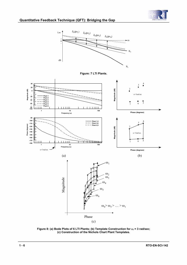
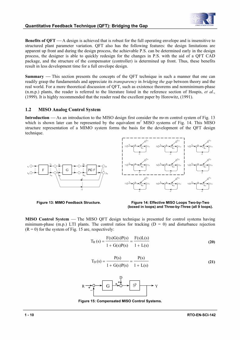
QFT Basics Consider the Control system of Fig. 6 where G(s) is a compensator, F(s) is a prefilter, and P is a nonlinear plant. To accomplish a QFT design for this system the nonlinear plant is described by a set of J m.p. LTI plants, i.e., P = {Pι(s)} (ι = 1,2,...,J), which define the structured plant parameter uncertainty. Note that for MIMO systems the elements pij of the mxm plant matrix P can be n.m.p. For MISO systems the discussion is restricted to m.p. plants. The magnitude variation, δP(jωi), is due to the plant parameter uncertainty which is depicted by the Bode plots of the LTI plants (see Fig. 7) for the example of Figs. 3 and 4. The J data points [log magnitude (Lm) and phase angle (φ)], for each value of frequency, ω = ωi, are plotted on the N.C. The contour that is drawn through the data points, for ωi, describes the boundary of the region that contains all J points. The contours are referred to as templates which represent the region of structured plant parametric uncertainty on the N.C. and are obtained for specified values of frequency, ω = ωi, within the bandwidth (BW) of concern. The six data points (Lm and φ) for the example of Fig. 3, for each value of ωi, are obtained as shown in Fig. 8a. These points are used to plot the templates, for each value of ωi as shown in Fig. 8b for ωi = 3 rad/sec and in Fig. 8c for other values of ωi. The system P.S. are represented by LTI transfer functions whose corresponding Bode plots are shown in Fig. 7 by the upper and lower bounds BU and BL, respectively.

PG(s)F(s) + -

R R L

L

Y

Figure 6: Compensated Nonlinear System.



Lm

+0-

dB

ω

BU

δP(jω1) δP(jω2)δP(jω3) δP(jω4)

BL

Figure: 7 LTI Plants.

40

20

0

-20-

40-

60-

80-100

Mag

nitu

de (d

B)

1 10 100

Plant 1Plant 2Plant 3Plant 4Plant 5Plant 6

Frequency (ω)

Frequency (ω)1 10 100

-180

-170

-160

-150

-140-130

-120

-110

-100

-90

Plant 1,2Plant 3,6Plant 4,5

Phas

e (d

egre

es)

ω=3rad/sec

Mag

nitu

de (d

B)

Phase (degrees)M

agni

tude

(dB

)

Phase (degrees)

ω=3rad/sec

ω=3rad/sec

1

2

34

56

1

2

34

56

(a) (b)

Phase

Mag

nitu

de

ω1

ω2ω3

ω4

ω5

ω6

ω6> ω5 > … > ω1

(c)

Figure 8: (a) Bode Plots of 6 LTI Plants; (b) Template Construction for ωi = 3 rad/sec; (c) Construction of the Nichols Chart Plant Templates.



QFT Design The tracking design objective is to synthesize a compensator G(s) of Fig. 6 which results in satisfying the desired P.S. of Fig. 5 and in the corresponding closed-loop frequency responses

shown in Fig. 9. This results in the δL(jωi) of Fig. 9, of the compensated system, being equal to or smaller than δP(jωi) of Fig. 7 for the uncompensated system and that it is equal or less than δR(jωi), for each value of ωi of interest; that is:

ιLT

)(jωδ)(jωδ)(jωδ iPiRiL ≤≤

The next step is to synthesize a prefilter F(s) of Fig. 6 which results in shifting and reshaping the TLι responses in order that they lie within the BU and BL boundaries in Fig. 9 as shown in Fig. 10.

+0-

dB

Lm

ω

BU

δL(jω1)δL(jω2)

δL(jω3) δL(jω4)

BL

δR(jω4)

δR(jω3)

δR(jω2)δR(jω1)

TLι

+0-

dB

Lm

ω

BU

BL

TRι

Figure 9: Closed-loop Responses: LTI Plants with G(s).

Figure10: Closed-loop Responses: LTI Plants with G(s) and F(s).

Therefore, the QFT robust design technique assures that the desired performance specifications are satisfied over the prescribed region of structured plant parametric uncertainty.

Insight to the QFT Technique The open-loop plant transfer function for the position control system of Fig. 6 is

a)s(s

Ka)s(s

Ka(s)P+′=

+=ι (7)

where K′ = Ka and ι = 1,2,…, J. The Lm variation due to the plant parameter uncertainty, for J = 6, is depicted by the Bode plots in Fig. 4. The loop transmission L(s) of the unity-feedback system of Fig. 6 is defined as

Lι(s) = G(s)Pι(s) (8)

The overall system control ratio TR, which includes the prefilter, is given by:

(s)L1

(s)F(s)L(s)TR

ι

ιι

+= (9)

for each ι plant and whose control ratio TLι is:

ι

ιι

L1

LRY

TL

L+

== (10)



Results of Applying the QFT Design Technique Proper application of the robust QFT design technique requires the utilization of the prescribed P.S. from the onset of the design process, the selection of a nominal plant Po from the J LTI plants, and the proper loop shaping of Lo(s) = G(s)Po(s) which results in obtaining a synthesized G(s) that satisfies the desired P.S. The last step of this design process is the synthesis of a prefilter that ensures that the Bode plots of all lie between the upper and lower bounds BU and BL.

ιRT

Insight to the Use of the Nichols Chart (N.C.) in the QFT Technique A review of the use of the N.C. and an insight as to how it applies to the QFT technique is now provided.

Open-Loop Characteristics − For the nominal plant Po(jω), the nominal loop transmission function is

Lm Lo = Lm GPo = Lm G + Lm Po (11)

Whereas for all other plants, P(jω), the loop transmission function is

Lm L = Lm GP = Lm G + Lm P (12)

Thus, for ω = ωi, the variation δP(jωi) in Lm L(jωi) is given by

δP(jωi) = Lm L(jωi) – Lm Lo(jωi) = Lm P(jωi) – Lm Po(jωi) (13)

and its phase angle variation is given by

∠∆P(jωi) = ∠L - ∠Lo = (∠G + ∠P) – (∠G + ∠Po) = ∠P - ∠Po (14)

The expression Lm P(jωi) = Lm Po(jωi) + δP(jωi), obtained from Eq. (13), is substituted into Eq. (12) to yield

Lm L(jωi) = LmG(jωi) + LmPo(jωi) + δP(jωi) (15)

where δP(jωi), is the variation from the nominal point.

Closed-Loop Characteristics – The closed-loop system characteristics are obtained, for a given G(jω) and Po(jω), from the plot of Lm Lo(jω) vs. ∠Lo shown on the N.C. in Fig. 11. Also, is shown a plot of a template, ℑ P(jωi), whose contour is based upon the data obtained for ω = ωi from Fig. 4. The template represents a region of plant parameter uncertainty for ωi as expressed mathematically by Eqs. (14) and (15). From the loop transmission plot and its intersections with the M- and α-contours (note: the α contours are not shown), the closed-loop frequency response data may be obtained for plotting Mo and α vs. ω. In Fig. 12 a plot of Mo vs. ω is shown, where

)(j1

)(j

)(j

)(j)(j)(jM

o

oo

ω

ω

ω

ωωαω

L

L

R

Y

+==∠



-24 -20 -16 -12 -8 -4 0 4 8

12 16 20 24 28

0 ° -20 ° -40 °-60 ° -80 ° -100 ° -120 ° -140 ° -160 ° -180 °

12 8 6 5 4 3 2

1dB

0.5 0.35

-24

-18

-12 -9 -6 -5 -4 -3 -2

-1dB

0dB -0.25

-0.5

A

B C

D

L o ( j ω )

T P ( j ωi)

Lm α

Lm β

L o ( j ω i )

L E ( j ω i ) = G(jωi)P(jωi)E

dB

Lm T(jω)

ω

Lm Tmax

0

-2

-4

-6

Lm Tmin

Lm TE

Lm M0 (jω) = Lm Tmin (jωi)

E

C

A

ωi

δR (jωi) = 4 dB

Figure 11: Nominal Loop Transmission Plot with Fig. 11.

Figure 12: Closed-loop Responses obtained from Plant Parameter Area of Uncertainty.

Parametric Variation N.C. Characteristics – As an example consider that for Eq. (8) G = 1∠0o. If point A on the template in Fig. 11 represents Lm Po vs. ∠Po, then a variation in P results in a horizontal translation in the angle of P, given by Eq. (14) and in a vertical translation in the Lm value of P, given by Eq. (15). The translations are shown in Fig. 11 at points B, C, and D. The variation δP(jωi) of the plant, and in turn L(jωi), from the nominal value for ω = ωi, over the range of plant parameter variation, is described by the template ℑP(jωi) shown in Fig. 11. For example, point A on the template represents the nominal plant P = Po(jωi). Its corresponding closed-loop frequency response is:

Lm MA = Lm β = -6 dB (16)

For P(jω) = Pι(jω): point C in Fig. 11, its corresponding closed-loop frequency response is

Lm MC = Lm α = -2 dB (17)

These values are plotted in Fig. 12. Note that point A represents the minimum value of Lm M(jωi) at ω = ωi, i.e., Lm Tmin = [Lm M(jωi)]min = Lm β (18)

Point C represents the largest value of Lm M(jωi) at ω = ωi, i.e.,

Lm Tmax = [Lm M(jωi)]max = Lm α (19)

For the range of plant parameter variation described by the template the maximum variation in Lm M, denoted by δL(jωi), for this example is

dB46)(2LmLm)i(jL =−−−=−= βαωδ

When Lo(s) is properly synthesized then δL(jωi) ≤ δR(jωi). Shown in Fig. 12 is point E, midway between points A and C, that corresponds to point E in Fig. 11 which lies within the variation template ℑP(jωi). This procedure is repeated to obtain the maximum variation δL(jωi) for each value of frequency ω = ωi within the desired BW (see Fig. 12). From this figure it is possible to determine the variation in the control system’s figures of merit due to the plant’s parameter uncertainty. This graphical description of the effect of plant parameter uncertainty on the system’s performance is the basis of the QFT technique.



Benefits of QFT A design is achieved that is robust for the full operating envelope and is insensitive to structured plant parameter variation. QFT also has the following features: the design limitations are apparent up front and during the design process, the achievable P.S. can be determined early in the design process, the designer is able to quickly redesign for the changes in P.S. with the aid of a QFT CAD package, and the structure of the compensator (controller) is determined up front. Thus, these benefits result in less development time for a full envelope design.

Summary This section presents the concepts of the QFT technique in such a manner that one can readily grasp the fundamentals and appreciate its transparency in bridging the gap between theory and the real world. For a more theoretical discussion of QFT, such as existence theorems and nonminimum-phase (n.m.p.) plants, the reader is referred to the literature listed in the reference section of Houpis, et al., (1999). It is highly recommended that the reader read the excellent paper by Horowitz, (1991).

1.2 MISO Analog Control System Introduction As an introduction to the MISO design first consider the m×m control system of Fig. 13 which is shown later can be represented by the equivalent m2 MISO systems of Fig. 14. This MISO structure representation of a MIMO system forms the basis for the development of the QFT design technique.

. . .

. . . . . .

. . . . . .

. . . F G P

. . .

v 1 u 1 w 1 y 1 r 1 y m r m v m u m w m

- 1

- 1

ε P

c11

f11 g1r1 y11q11

-1

c13

f13 g1r3 y13q11

-1

c12

f12 g1r2 y12q11

-1

c21

f21 g2r1 y21q22

-1

c23

f23 g2r3 y23q22

-1

c22

f22 g2r2 y22q22

-1

c31

f31 g3r1 y31q33

-1

c33

f33 g3r3 y33q33

-1

c32

f32 g3r2 y32q33

-1

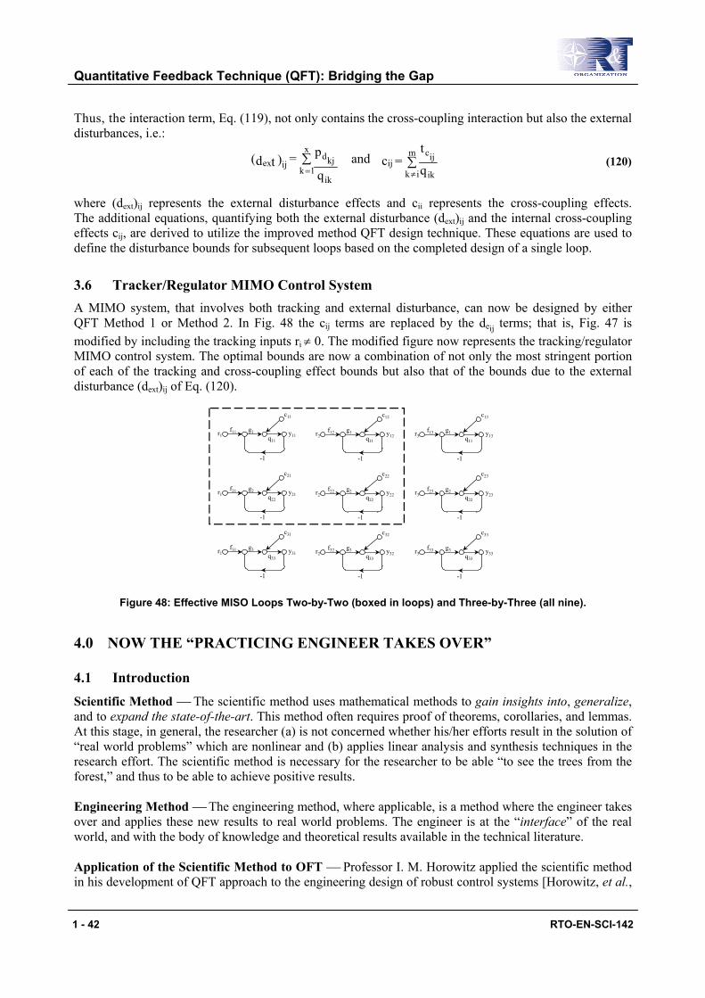
Figure 13: MIMO Feedback Structure. Figure 14: Effective MISO Loops Two-by-Two (boxed in loops) and Three-by-Three (all 9 loops).

MISO Control System The MISO QFT design technique is presented for control systems having minimum-phase (m.p.) LTI plants. The control ratios for tracking (D = 0) and disturbance rejection (R = 0) for the system of Fig. 15 are, respectively:

L(s)1

F(s)L(s)

G(s)P(s)1

s)F(s)G(s)P((s)TR

+=

+= (20)

L(s)1

P(s)

G(s)P(s)1

P(s)(s)TD

+=

+= (21)

P

D

G R _ + + +

Y

Figure 15: Compensated MISO Control Systems.

1 - 10 RTO-EN-SCI-142


The robust design objective is to design G(s) and F(s) of Fig. 15 for the plant having parameter uncertainty. The design procedure to achieve this objective is as follows:

Step 1: Synthesize tracking models

Step 2: Synthesize disturbance model

Step 3: Specify J LTI plant models (define uncertainty)

Step 4: Obtain templates at specified ωi (describes uncertainty)

Step 5: Select nominal plant Po(s)

Step 6: Determine stability contour (U-contour) on N.C.

Steps 7-9: Determine disturbance, tracking, and optimal bounds

Step 10: Synthesize nominal Lo(s) = G(s)Po(s) to satisfy all bounds and the stability contour in order to obtain

G(s) = Lo(s)/Po(s)

Step 11: Synthesize prefilter F(s).

Step 12: Simulate linear system (J time responses)

Step 13: Simulate with nonlinearities

Synthesize Tracking Models Based upon the FOM specifications [see Fig.5a] MP, tp, ts, and tr, for a unit step forcing function, underdamped and overdamped tracking models are synthesized.

Simple Second-order Models – Models are synthesized for an upper bound y(t)U and for a lower bound y(t)L that yield bounds between which the acceptable response y(t) must lie. For m.p. plants, only tolerance on |TR(jωi)| need be satisfied where for nonminimum-phase (n.m.p.) plants the tolerances on ∠[TR(jωi)] must also be satisfied.

Synthesized tracking control ratios – The tracking models are:

2n

2

2n

URs2s

a)/a)(s((s)T

ωςωω

++

+=

n Upper Bound (22)

))(s)(s(s

K(s)T

321LR

σσσ −−−= Lower Bound (23)

These models are synthesized so that in Fig. 5b for ωi > ωh δR(jωi) increases in order to simplify the process of synthesizing Lo(s) = G(s)Po(s). Note that the frequency bandwidth (BW), 0 < ω < ωh [see Fig. 5b] is determined by the −12 dB line.

Disturbance Models Based upon a unit step disturbance input (D of Fig. 15) the simplest disturbance model is:

|TD(jω)| = |Y(jω)/D(jω)| ≤ αp (maximum allowable magnitude of |TD|)

RTO-EN-SCI-142 1 - 11


Thus, the frequency domain specification is:

Lm TD(jω) < Lm αp over the BW

This results in only an upper bound.

J LTI Plant Models The following simple plant is chosen for illustrative purposes:

a)s(sK

)as(sKa

(s)P+′

=+

=ι (24)

where K′ = Ka, K ∈ {1, 10} and a ∈{1, 10}. The region of plant parameter uncertainty (see Fig. 16) which is described by the J LTI plants defined by points 1, 2, 3, 4, 5, and 6. These models define the region of plant parameter uncertainty as shown in the figure.

2 3 4

1 6 5

a

K

0

Region of plantparameter uncertainty

Kmax

Kmin

amin amax

Figure 16: Region of Plant Parameter Uncertainty.

Plant Templates of Pι, ℑP(jωi) The overall tracking control ratio of Fig. 15, where L = GP, is

+

=L1

LFTR

which yields

+

+=L1

LLmFLmTLm R

Subtracting Lm F from sides of the above equation yields:

+

−=∆L1

LLmTLm)T(Lm RR

The change in TR due to the uncertainty in P (F is LTI), is:

+

=−∆=L1

LLmF)LmT(Lm RR ιδ (25)

for ι = 1,2, … , J plants. The nominal loop transmission Lo and the prefilter F are designed (synthesized) so that the actual value of Lm T always lies between BU and BL of Fig. 5b. Thus, draw the templates that characterize the variation of plant uncertainty onto the Nichols Chart (N.C.) for various values of ωi over

1 - 12 RTO-EN-SCI-142


the BW. The six points on the boundary of the region of plant uncertainty are mapped onto the N.C. in Fig. 17 where 1 → A, 2 → B, 4 → C, 5 → D. Note that point 3 lies between B and C and point 6 lies between D and A. A curve is drawn through these points, as indicated in the figure, and the shaded area is labeled ℑP(j1). Templates for other values of ωi are obtained in the same manner.

T P (j1)

C B

A

D

K=10

a=10

a=1

K=1

20 17

dB

0

- 3 - 180°

- 90° - 135°

- 0.04 dB

Phase

dB

Figure 17: N.C. Characterizing Eq. (7) over the Region of Uncertainty.

Characteristic of Templates The templates of Fig. 8b have the following characteristics: (1) starting from low values of ωi the angular width of the templates become larger; (2) for increasing values of ωi the templates then become narrower; and (3) they eventually approach a straight line of height V dB [see Eq. (27)].

Nominal Plant Any of the J plants can be chosen as the nominal plant Po. One can select, if specifications permit, a plant whose N.C. point is always at the lower left corner for all templates. In Houpis, et al. (1999) general guidelines are given in Chapter 9 for selecting the nominal plant.

U-Contour (Stability Bound) The value of Mm (see Fig. 5b) identifies the desired maximum overshoot for a closed-loop system. Thus, from this figure the bound MP ≅ Mm is chosen. This bound identifies the M-contour on the N.C. Mm = ML (see Fig. 5). This contour establishes a region that can not be penetrated by the templates and by Lo(jω).the dominating constraints on Lo(jω). The top portion (efa) of the ML contour becomes part of the U-contour (See Fig. 18). The limiting value of the plant transfer function, for a large problem class, approaches

λωK

)](j[lim =∞→

ωω

P (26)

where λ is the excess of poles over zeros of P(s). The plant template, for this problem class, approaches a vertical line of length equal to

(27) dBVKLmKLm]PLmP[Lmlim minmaxminmax =−=−=∆∞→ω

The nominal plant, for this example, is chosen at K = Kmin (point 1 of Fig. 16) which results in the U-contour abcdefa of Fig. 18.

RTO-EN-SCI-142 1 - 13


dB

-180° -90°

M-contour (Lm ML)+f

a

b

c

d

e

g

0

_V

U-contour

V

V

Bh- boundary

Figure 18: U-contour Construction (Stability Contour).

Optimal (Composite) Bounds Bo(jωi) on Lo(jωi) By applying the procedures given by Houpis, et al., (1999), the tracking bounds BR(jωi), and the disturbance bounds BD(jωi) are determined which in turn result in obtaining the composite bounds Bo(jωi) that become the bounds required in synthesizing Lo( jωi).

Tracking Bounds on Lo – The determination of the tracking bounds BR(jωi) requires that

dB)(jωδ)(jω∆T)(jωδ iRiRiL ≤=

be satisfied for all Lι(jωi) [see Figs. 5b, 9 and 10]. The procedure for determining these bounds is based on a nominal plant Lo, is as follows: at each specified value ωi and the use of the corresponding template (or CAD), see Fig. 19, the nominal point A on the template is moved up or down along the N.C. angle grid line without rotating the template; this template is moved until it is tangent to two M-contours whose difference in their M values is essentially equal to δR. When this condition is achieved, the location of the nominal point on the template becomes a point on the bound BR(jωi). This, procedure is repeated on sufficient angle grid lines to provide enough points to draw BR(jωi) and is repeated for all values of frequency for which templates have been obtained.

--180º

φx

BR(jω)

AD

B

C

A'

D'

B'

C'

0

Lmβ dB

-90º

Lm α dB

ML - contour dB

+

– Figure 19: Graphical Determination of BR(jωi).

1 - 14 RTO-EN-SCI-142


Disturbance Bounds Procedure (MISO System) – Two cases of disturbance bounds are considered as indicated in Fig. 20. These cases are: Case 1 [d2(t) = Dou-1,(t), d1(t) = 0] and Case 2 [d1(t) = Dou-1,(t), d2(t) = 0].

P

D 1 D 2 G F R Y

_ + + + + +

Figure 20: A Feedback Structure.

Case 1: From Fig. 20, the disturbance control ratio for input d2(t) is

L1

1(s)TD

+= (28)

Substituting L = 1/l into Eq. (28) yields:

l

l

+=

1(s)TD (29)

that has the mathematical format required to use the N.C. Over the specified BW it is desired that |TD(jω)| << 1, which results in the requirement, from Eq. (28), that |L(jω)| >> 1 (or |l( jω)| << 1), i.e.,

)(j)(j

1)(jD ω

ωω l=≈

LT (30)

A time-domain tracking response based upon r(t) = u-1(t) often specifies a maximum allowable peak overshoot Mp, which in the frequency domain this specification may be approximated by:

pmRR MM)ω(j

)ω(j)jω()jω( ≈≤==

R

YTM (31)

The corresponding time- and frequency-domain disturbance response characteristics, based upon the step disturbance forcing function d2(t) = u-1(t), are determined in the same manner, i.e.,

xpD ttforαd(t)

y(t)(t)m ≥≤= (32)

and

pmDD αα)ω(j

)ω(j)jω()jω( ≈≤==

D

YTM (33)

The disturbance control ratio of Eq. (29) must have the desired characteristic over the desired BW 0 ≤ ω ≤ ω2 for which L(jω) >> 1 and l( jω)<< 1. Thus, Eq. (31) applies within this BW region. Consider for a given plant L(s) that its plot of Lm L vs ∠L is shown in Fig. 21. The plot is tangent to the Lm M = 0.5 dB contour at ω = ωm. Table 1 contains data for two points on the Nichols plot of Fig. 21. Also, shown is the plot of Lm l( jω) vs. ∠ l for these two points.

RTO-EN-SCI-142 1 - 15


-12

-8

-4

0

4

8

12

16

20

24

28

1286543

2

1dB

0.5

0.35

-12

-9

-6

-5

-4

-3

-2dB

-1

0dB-0.25

-0.5

D

B

CA

D

Lm Lω1

ω2

ωm

T

βABβABP(jωi)

1ω

Atte

nuat

ion,

dB

T

Consider that equal dB diffe

This template location showshown in this for the same frof Lm [1/P(jωreflecting the it up or downLm [1/P(jωi)],

(a)

where for 1/P,

1 - 16

LTL m

-80°-100°-120°-140°-160°-180°-200°-220°-240°-260°280°-300

A

B

CβCDβCD

2ωb

ω1ωa

Phase angle, φ, deg

lL

-270° -90°

l

Figure 21: Regular Nichols Chart.

Table 1: Data Points for a Nichols Plot

ω Lm L ∠L Lm l ∠l

ω1 21 -96o -21 96o (or –

ω2 15 -98o -15 98o (or –

the template ℑP(jωi) for a given plant P having uncertarences along its A-B and C-D boundaries, i.e., for a given

)PLmP(Lm)PLmP(Lm DCAB =−∆=−∆

is arbitrarily set on the N.C. as shown in Fig. 21. The dn in Fig. 21 is given in Table 2. The plot of Lm l(jω) figure. The template of the reciprocal, Lm [1/P(jωi)], is aequency as for the template of Lm P(jωi) and for the angi)] is the same as the template of Lm P(jωi) but is rota

template of Lm P(jωi) about the −180o axis, “flipping it so that it lies between −5 and −20 dB. For the arbi note that:

oooCD

ooooAB

10080180180β

60120180180β

=−=∠+=

=−=∠+=

P

P

the corresponding angles are

ooCD

oCD

ooAB

oAB

100180β180)(1/P

60180β180)(1/P

=−−=−−=∠

−=−−=−−=∠

P(jωi)P(jωi)

-24

-20

-16

-24

-18

m
0°-20°-40°-60°
L
-°
lι ι

264o) 262o)

in parameters, for a given ωi, has ∠P(jωi),

dB10

ata corresponding to the template vs. ∠l for these 2 points is also rbitrarily set on the NC in Fig. 21 les of Table 1. Note, the template ted by 180o. It is located by first over” vertically, and then moving trary location of the template of

o

o

o

280

240

−

RTO-EN-SCI-142


(b) The templates of Lm P(jωi) are used for the tracker case: T = L/(1 + L) where L = GP.

(c) The templates of Lm [1/P(jωi)] used for the disturbance rejection case: TD = 1/(1 + L) = l/(1 + l) where l = 1/GP = 1/L.

Table 2: Data Points for the Templates of Fig. 21

Points ∠P ∠1/P A,B -120o 120o (or –240o) C,D -80o 80o (or -280o)

Since Lm L is desired for the disturbance-rejection case of Eq. (28) then Eq. (29) must be utilized to determine the corresponding disturbance bounds. Thus, the N.C. of Fig. 21 is rotated 180o and is redrawn in Fig. 22 in order to determine the disturbance boundary BD(jωi) for L(jωi) = 1/l(jωi) on this rotated N.C. Since Lm l(jω) = Lm [1/L(jω)] = − Lm L(jω), then a negative value of Lm l yields a positive value for Lm L as shown in Fig. 22. Since L = KL′ = 1/l , then

(34) )(j'K)(j 1 ωω ll −=

l0° -20° -40° -60° -80° -100° -120° -140° -160° -180° -200° -220° -240° -260° -280° -300°

1286543

2

1dB

0.5

0.35

-24

-18

-12

-9

-6

-5

-4

-3

-2dB

-1

0dB-0.25

-0.5

A

B

C

D

βCD

ω2

ωb

ω1

ωa L

280°or

-80°

240°or

-120°

(Note: Use the negative angle for L since n > w)L = 1/l

24 dB

18 dB

12 dB

For - Lm TD or BD(jωi) evaluationl

- 24

20-20

Lm LL

/l

l

l

Phase angle, φ, deg

Figure 22: Rotated Nichols Chart.

If l ′ ( jω) is given and it is required to determine K-1 to satisLm l ′ ( jω) vs. ∠l′( jω) must be raised or lowered until it is tangent to theThe amount ∆ by which the plot is raised or lowered yields the value of K, i.ethe same procedure used for obtaining the tracking bounds, except that the a

The rotated N.C. is used to determine directly the disturbance boundaries Bthe simple plant of this design example corresponds to the nominal plan

RTO-EN-SCI-142

m

-

-

1

1

2

2

2

fy E Lm α., Lmdjust

D(jωt para

42m

16

12

8

4

0

-4

-8

-12

-16

-20

-24

-28

16

12

-8

-4

0

4

8

2

6

0

4

8

Attenuation, dB

q. (33), then the plot p-contour (|TD|max = αm).

K-1 = ∆. Note, that this is ment in Lm l ( jω) is K-1.

i) for LD(jωi). Point A for meters and is the lowest

1 - 17


point of the template ℑP(jωi). This point is again used to determine the disturbance bounds BD(jωi). The lowest point of the template must be used to determine the bounds and, in general, may or may not be the point corresponding to the nominal plant parameters. Based upon Eqs. (28) - (30)

(35) dB0)(jLm]Lm[1Lm iD >−≥+=− ωαLT

where α(jωi) < 0. Since |L| >> 1 in the BW, then

(36) )(jω)(jωLmLmLm iDiD δα −=−≥≅− LT

In terms of L(jωi), the constant M-contours of the N.C. can be used to obtain the disturbance performance TD. This requires the change of sign of the vertical axis in dB and the M-contours, as shown in Fig. 22. The procedure for determining the boundaries BD(jωi) is given by Houpis, et al., (1999).

Case 2 [d1(t) = D0u-1(t), d2(t) = 0]: The disturbance control ratio for this case (see Fig. 20) is:

)(j(j1

(j)(jD

ωω

ωω

)PG

)PT

+= (37)

This equation, assuming point A of the template (Fig. 23) represents the nominal plant Po, is multiplied by Po/Po and is rearranged to obtain:

W

P

LP

PP

GPP

PP

GP

P

PT o

oo

o

oo

o

o

oD 1

1=

+=

+=

+=

(38)

where W = (Po/P) + Lo. From Eq. (38), set Lm TD = δD = Lm αp and obtain

(39) Do δPLmWLm −=

Templates are drawn in polar coordinates for each value of ωi. Shown in Fig. 23 is a template for ω = ωi. From Eq. (39) evaluate |W(jωi)| for ω = ωi. This magnitude is used in conjunction with the following equation

)(jω)](jω)/(jω[)(jω ioiioi LPPW +=

to obtain a graphical solution for Bd(jωi) (see Fig. 24). Thus, the N.C. bounds for the specified values of ωi are given by:

BD(jωi) = Lm Bd(jωi) and ∠ BD(jωi) = φ − 180o

A

D

B C

P O P T

1 0 °

- 90 °

Figure 23: Template in Polar Coordinates for ω = ωi .

1 - 18 RTO-EN-SCI-142

A D

B C

-170 ° -160 °

-150 ° -140 ° -130 °

| W ( j ω i )| Q - contour | W ( j ω i )| - B d ( j ω i )

φ

P O ( j ω i ) P ( j ω i ) T

2 1

j1

-180 °

B d

= φ

- 180 º

| W ( j ω i )|

Figure 24: Graphical Evaluation of Bd(jωi).

Optimal Bounds − The optimal bound Bo(jωi) for the case shown in Fig. 25a is composed of the portions of BR(jωi) and BD(jωi) that have the largest dB values. For the case shown in Fig. 25b the outermost portions of BR(jωi) and BD(jωi) becomes the perimeter of Bo(jωi) (yields the greatest interior area). For example, the synthesized Lo(jωi) must lie on or just above the bound Bo(jωi) of Fig. 25a.

Bo(jωi)BR(jωi)

BR(jωi)

BD(jωi)

Bo (jωi)

BR (jωi)BD(jωi)Bo (jωi)

BR (jωi)BD(jωi)

Bo (jωi)

(a) (b)

Figure 25: Composite Bo(jωi).

Synthesizing (or Loop Shaping) The shaping of Lo(jω), the dashed curve shown in Fig. 26 is achieved as follows: (1) a point such as Lm Lo(j2) must be on or above the U-contour and BR(j2); (2) to satisfy the performance specifications Lo(jωi) cannot violate (intersect) the U-contour; (3) Lo should closely follow the U-contour up to 40 r/s and must stay below it above 40 r/s; and for this example it must be at least a Type-1 function with at least one pole at the origin. In synthesizing the rational function Lo(s) that satisfies the above involves building up the function:

(40) ∏==

=w

0kkkook)(jo )](jG[K)(P)(jLL ωωωω j

where for k = 0, Go = 1∠0o, and . In order to minimize the degree of G(s) assume initially that

Lo(jω) = Po(jω) in Eq. (40) and then build up Lo(jω) term-by-term so that the point Lo(jωi) lies on or above the corresponding Bo(jωi) and it stays just outside the U-contour. The design of a proper Lo(s) guarantees only that the variation δL is less than or equal to δR(jωi). Once a proper Lo(s) is synthesized then the compensator is given by G(s) = Lo(s)/Po(s). For this example Lo(jω) slightly intersects the U-contour. Since the QFT technique has the inherent characteristic of resulting in an over-design, thus for the first trial design no effort is made to fine tune G(s). If the simulation results are not satisfactory then Lo is fine tuned.

kw

kK

0K

=Π=

RTO-EN-SCI-142 1 - 19


-180°

8db

16db

24db

0db

-8db

-16db

-24db

-140° -100° -60°

Bo(j1)

Bo(j2)

Bo(j3)

Bo(j4)

Bo(j6)

Bo(j10)

Bo(j20)

ω=1

ω=2

ω=3

ω=5

ω=10

ω=20

ω=30

ω=40ω=60

ω=100

U-contour(StabilityBound)

LmLo(jω)

LmLo(jω)

A

ω=50

[B0(jω)] ω≥ωh=40

Figure 26: Shaping of Lo(jω) on the Nichols Chart for the Plant of Eq. (23).

Prefilter Design F(s) The design of Lo(s) guarantees only that the variation in |TR(jω)| is:

LmTR(jω)max, − Lm TR(jω)min < δR(jω)

Thus, the design procedure involves positioning

(s)L1

(s)L(s)T ιL

ι

ι

+= (41)

so that it lies between Bu and BL (see Fig. 5b) for all J plants. The filter design procedure is as follows:

Step 1: Place the nominal point, for this example Point A, of ωi on the plant template on to the Lo(jωi) point of the Lo(jω) curve (see Fig. 27).

-90

A

B

D

C

-180°0db

dB

Lm Tmin

Lo(j

Lo(jω)

U - contour

Lm Tmax

Desired M L - contour

M - contours

Figure 27: Prefilter Determina

1 - 20

TP(jωi)

° Phase

ωi)

tion.

RTO-EN-SCI-142


Step 2: Traversing the template, obtain the values of Lm Tmax and Lm Tmin values of Eq. (41).

Step 3: Obtain the data points within the desired BW and in conjunction with the data from Fig. 5(b) plots of Fig. 28 are obtained.

+0-

dB

Lm

ω

LmTRL- LmTmin

0db/dec

-20db/dec

-40db/dec

LmTRU- LmTmax

Figure 28: Frequency Bounds on the Prefilter F(s).

Step 4: Utilizing Fig. 28, the straight line Bode technique is applied and with the condition

(42) 1F(s)lim0s

=→

for a step forcing function satisfied an F(s) is synthesized as shown, in dashes, that lies within the upper and lower plots in Fig. 28.

Design Procedure for the QFT Technique for M.P. Plants

Step 1: Synthesize the tracking model control ratios TR(s): TRU(s) TRL(s)

Step 2: Synthesize the disturbance-rejection model control ratios TD(s)

Step 3: Specify J LTI plant models (define the plant uncertainty)

Step 4: Obtain templates of P(jωi) for specified ωi (describes uncertainty) within the BW

Step 5: Select a nominal plant Po(s)

Step 6: Determine the stability contour (U-contour) on N.C.

Step 7: Determine the disturbance bound BD(jωi) on N.C.

Step 8: Determine the tracking bound BR(jωi) on N.C.

Step 9: Determine the optimal bounds Lm Bo(jωi) vs. for values of ωi

Step10: Synthesize the nominal Lo(jωi) = G(jω)Po(jω) that satisfies all the bounds and the stability contours and then obtain G(s) = Lo/Po(s)

Step 11: Synthesize the prefilter F(s)

Step 12: Simulate the LTI system (J time responses)

Step 13: Simulate with the nonlinearities

RTO-EN-SCI-142 1 - 21


1.3 MISO Discrete Control System A MISO QFT digital control system is shown in Fig. 29. The z-domain equations that describe this system are:

)(P)1(s

P(s))(1)(PG)(P Ze1Z1ZZZOZz

−− === (43)

GL(z) zo=

(s)Pe ≡

)(P Ze ≡s

P(s

_+T F*(s)r(t)

R*(s) V*(s) E*(s) X*

Y*(s)

R(s)

x(ke (kT)v(kT)r(kT)

y(kT)

G*(s)1

Filter Controller

Figure 29: A MISO Sampl

For a unit step disturbance, D(s) = 1/s:

P(s)D(s)Pe =

PD(z) = [P(s Z

L(z)TF(z)L(z)1

F(z)L(z)(z)T RR ′=

+=

where

(z)'TR =

YL(z)1

PD(z)R(z)

L(z)1

L(z)F(z)Y(z) =

++

+=

1.4 Pseudo-Continuous-Time (PCT) SystemIntroduction The PCT, a digitization (DIG) tecontroller, D(z), in the s-domain [Houpis, et al. (199(controller) D(s) is transformed into the z-domain

1 - 22

Z

(z)P(z)G1

sP(s) (44)

) = [ ](s)eP
Z
(s)

T)

ed-

(s)

)D(

(z)

1L+

(zR

ofchn9)] b

Z Z

P(s)Y(s)

ZOH

T

+

+

M(s)

d(t), D(s)

W(s)

m(t) w(t) y(t)

Y*(s)

y*(t)

TPlant

data Control System.

(45) P(s)/s=

s)] (z)Pe=

L(z)1

PD(z)(z)Tand D +

= (46)

L(z)(z)

(z)Y(z)R(z)T(z)Y) DRD +=+ (47)

a Digital Control System ique, allows the QFT design of the z-domain . That is, the synthesized s-domain compensator y use of the Tustin transformation, a bilinear

RTO-EN-SCI-142


transformation, to obtain D(z). The advantage of this approach, especially when the plant is m.p., eliminates dealing with a n.m.p. plant when doing the analysis and design in the w′-plane and the associated problem in satisfying the w′-domain stability bounds. Note: in Fig. 29 D(z) = G1(z).

Another important advantage is, with sampling times T < 0.01 s that are know available, the warping effect that is discussed later on, is minimal thus the s-domain characteristics are transformed into the z-domain assuring that the robust QFT design is achieved in the z-domain. The transformation into the s-domain enables the use of the MISO QFT analog design technique to be used, with minor exceptions, to design the controller D(s). If the s-domain simulations satisfy the desired P.S. then by use of the bilinear transformation the controller G(z) is obtained. With this synthesized z-domain controller a discrete-time domain simulation is performed to verify the goodness of the QFT design.

Bilinear Transformations The Tustin transformation, a bilinear transformation, transforms an s-domain function into the z-domain or vice-versa. A function of z is substituted for sq in implementing the Tustin transformation. This function is:

q

1

1q

z1

z1

T

2s

−

−

+

−= (48)

The advantages of the Tustin algorithm are: it is easy to implement, the accuracy of the Tustin z-domain transfer function is good compared with the exact z-domain transfer function, and the accuracy increases as the sampling frequency fs increases or the sampling time T decreases. The Tustin bilinear transformation for q = 1 is defined as:

1z1z

T2

z1z1

T2s

1

1

+−=

+−≡

−

− (49)

and can be equated to the trapezoidal integration (s-1) method.

Mapping Characteristics − For the s- to z-plane mapping Eq. (49) is rearranged to yield

sT/21

sT/21z

−

+= (50)

Utilizing the mathematical expression

a1j2tanea1a1 −=

−+

and letting in Eq. (50) the following expression for z is obtained: spω̂js =

T/2spω̂1j2tan

sp

spe

T/2ω̂j1

T/2ω̂j1z −=

−

+= (51)

Where for the exact Z-transform the expression for z is , where ωsp is an equivalent s-plane frequency. This expression is substituted into Eq. (51) to obtain:

Tspjωez =

−=

2Tω̂j2tanexpe sp1Tspjω (52)

RTO-EN-SCI-142 1 - 23


Equating the exponents yields:

2Tωtan

2Tω sp1sp

)−= (53)

or

2

Tspω2

Tspωtan

)

= (54)

When ωspT/2 < 17o, or ≈ 0.30 rad, then

(55) spsp ω̂ω ≈

Thus, in the frequency domain the Tustin approximation is good for small values of ωspT/2, that is, minimal warping is achieved for the imaginary component.

The warping of the real pole component is determined as follows. Substitute and into Eq. (50) to yield:

Tσspez = spσ̂s =

T/2σ̂1

T/2σ̂1Tσesp

spsp

−

+= (56)

Replacing by its exponential series and dividing the numerator of the right-hand side by its denominator in Eq. (56) results in the expression

Tspσe

( )

T/2σ̂1Tσ̂1

2TσTσ1

sp

sp2

spsp

−+=+++ L (57)

If |σspT | >> (σspT )2/2 (or 1 >> |σspT/2|) and 1 >> T/2σ̂sp , then minimal warping occurs and

T2σσ̂ spsp <<≈ (58)

When Eqs. (55) and (58) are satisfied the Tustin approximation in the s-domain is good for small magnitudes of real and imaginary components of the variable s. The shaded area in Fig. 30 represents the allowable location of the dominant poles and zeros in the s plane for a good Tustin approximation. That is, only the dominant poles and zeros of the open-loop transfer function, that determine the achievement of the desired P.S., need be in the shaded area. Due to the properties and its ease of use, the Tustin transformation is employed for the digitization (DIG) technique. Figure 31a is the mapping of

= 2(tan ωspT/2)/T [see Eq. (54)] and Fig. 31b illustrates the warping effect of a pole (or zero) when the approximations are not satisfied. ω̂

1 - 24 RTO-EN-SCI-142


- 0.1T

ωs2

j = 3.14T

j

0.6114T

j

0.6114T

-j

3.14T

-j

σ

jω

s-plane

- 2T

Figure 30: Allowable Location (shaded area) of Dominant Poles and Zeros in S-plane for a good Tustin Approximation.

1.0 (45°)0.5774 (30°)

0.3057 (17°)

0.7890.5230.298R

adia

ns

s-plane values

Tustin value, rad (deg)

ωspT/2

ωspT/2

π/2

−π/2

s-plane

σ

Warping Direction of ωsp

Warping Direction of σsp

jωspjωsp

jωs/2

σsp σsp

(a) (b)

Figure 31: Map of ω = 2(tan ωspT/2)/T. (a) Plot of Eq. (52) and (b) Warping Effect. ˆ

Characteristic of a Bilinear Transformation − In general the bilinear transformation transforms an unequal-order transfer function (ns ≠ ws) in the s-domain into one for which the order of the numerator is equal to the order of its denominator (nz = wz) in the z-domain. This characteristic must be kept in mind when synthesizing G(s) and F(s).

Introduction to PCT System: A DIG Technique A satisfactory pseudo-continuous-time (PCT) model is obtained for the sampled-data (S-D) system shown in Fig. 32. The PCT approximation of the sampler and the ZOH units of Fig. 32 are shown in Fig. 33b. The multiplier 1/T attenuates the fundamental frequency of the sampled signal and all of its harmonics. These approximations are represented by the linear continuous-time unit GA(s), as shown in Fig. 33c. The dominant poles and zeros of the PCT model should lie in the shaded area of Fig. 30 for a high level of correlation with the S-D system. The frequency component E*(jω) of the sampled signal e*(t) represents E(jω) of the continuous-time signal e(t) multiplied by 1/T, where all the side-bands of e*(t), are also multiplied by 1/T, are attenuated due to the low-pass filtering characteristics of a S-D system.

RTO-EN-SCI-142 1 - 25


Gx(s)C(s)R(s)

_+ ZOHE*(s) M(s)

G(s)

E(s)T E(z)

Plant

T

C*(s)

C(z)

Gz(z)

Figure 32: The Uncompensated Sampled-data Control System.

Gzo(s)M(s)E*(s)E(s)

T

M(s)E(s)Gpa(s)1

T

Samplerapproximation

ZOHapproximation

(a) (b)

Gx(s)R(s) C(s)

_+ GA(s)E(s) M(s)

Gpc(s)

(c)

Figure 33: (a) Sampler and ZOH; (b) Approximations of the Sampler and ZOH; (c) the Approximate Continuous-time Control System Equivalent of Fig. 32.

Using the first Pade′ approximation, the transfer function of the ZOH device, when the value of T is small enough, is approximated as follows:

(s)G2Ts

2Tse1(s)G pa

TsZO =

+≈−= (59)

where the transfer function Gpa(s) is used to replace Gzo(s) as shown in Fig.33b and c. Thus, the sampler and ZOH units of the S-D system are approximated in the PCT system of Fig. 33c by the transfer function:

2Ts2(s)G

T1(s)G paA

+== (60)

Since Eq. (60) satisfies the condition limT→0GA(s) = 1 it is an accurate PCT representation of the sampler and ZOH units. That is, it satisfies the requirement that as T → 0 the output of GA(s) must equal its input and in the frequency domain as ωs → ∞ (T → 0) the primary strip becomes the entire frequency-spectrum domain, the representation for the continuous-time system.

A Simple PCT Example As an illustration of the effect of the value of T on the validity of the results consider the S-D closed-loop control system of Fig. 32 where

5)1)(ss(s(s)G x

xK

++= (61)

The closed-loop system performance is determined for three values of T in both the s- and z-domains [DIG technique vs the direct (DIR) technique (the z-plane analysis)]. For each value of T and by use of the

1 - 26 RTO-EN-SCI-142


root-locus technique the dominant closed-loop poles are determined for a ζ= 0.45. Table 3 presents the required value of Kx and the time-response characteristics for each value of T. Note, (a) for T ≤ 0.1 s a high level of correlation exists between the DIG and DIR models, and (b) for T ≤ 1 s still a relatively good correlation exists. (The designer needs to specify, for a given application, what is considered to be a “good correlation.”)

Table 3: Analysis of a PCT System representing a Sampled-data Control System for ζ = 0.45

Method T,s Plane Mp Tp,s Ts,s DIR z 1.202 4.16 9.53 DIG

0.01 s 1.206 4.11 9.478

DIR z 1.202 4.2+ 9.8+

DIG 0.01

s 1.203 4.33- 9.90+

DIR z 1.199 6 13-14 DIG

1.0 s 1.200 6.18 13.76

The MISO PCT QFT Approach The PCT System of the digital control system of Fig. 29 is shown in Fig. 34a. Note that the sampler sampling the forcing function and the sampler in the system’s output y(t) are replaced by a factor of 1/T. The diagram in Fig. 34a is simplified to the one shown in Fig. 34b and is the structure that is used for the QFT design. The QFT design technique can now be applied to this PCT system.

PCT Design Summary − Once a satisfactory Dc(s) [= G1(s)/T] (see Fig. 34b), whose order of the numerator and denominator are, respectively, ws and ns, has been achieved, then (a) if ns is equal to or greater than ws + 2 then the exact Z-transform is applied to obtain the discrete controller Dc(z); or (b) if ws < ns < ws + 2 then ns − ws non-dominant zeros need to be added to Dc(s) before applying the Tustin transformation to obtain [Dc(z)]TU. As a final check, before simulating the discrete design, obtain the Bode plots of Dc(s)|s = jω and . If the plots essentially lie on top of one another, within the

desired BW, then the discrete-time system response characteristics are essentially the same as those for the PCT system response. If the plots differ appreciably this implies that warping has occurred and the desired discrete-time response characteristics may not be achieved (depending on the degree of the warping). If the warping is not negligible a smaller value of T needs to be selected if allowable.

ωjezc |(z)D =

P(s)Y(s)_+F(s) +

+r(t)

V(s) E(s) X (s) M(s)

d(t), D(s)

B(s)

R(s) W(s)

x(t)e (t)v(t) m(t) w(t) y(t)

b(t)

G1(s)

1T

1T

Gpa(s)

P(s)Y(s)

_+F(s) +

+V'(s) E' (s) X (s) M(s)

D(s)

B' (s)

R(s) W(s)G1(s) Gpa(s)1

T

Dc(s)

(a)

(b)

Plant

Controller

Figure 34: The PCT Equivalents of Fig. 29.

RTO-EN-SCI-142 1 - 27


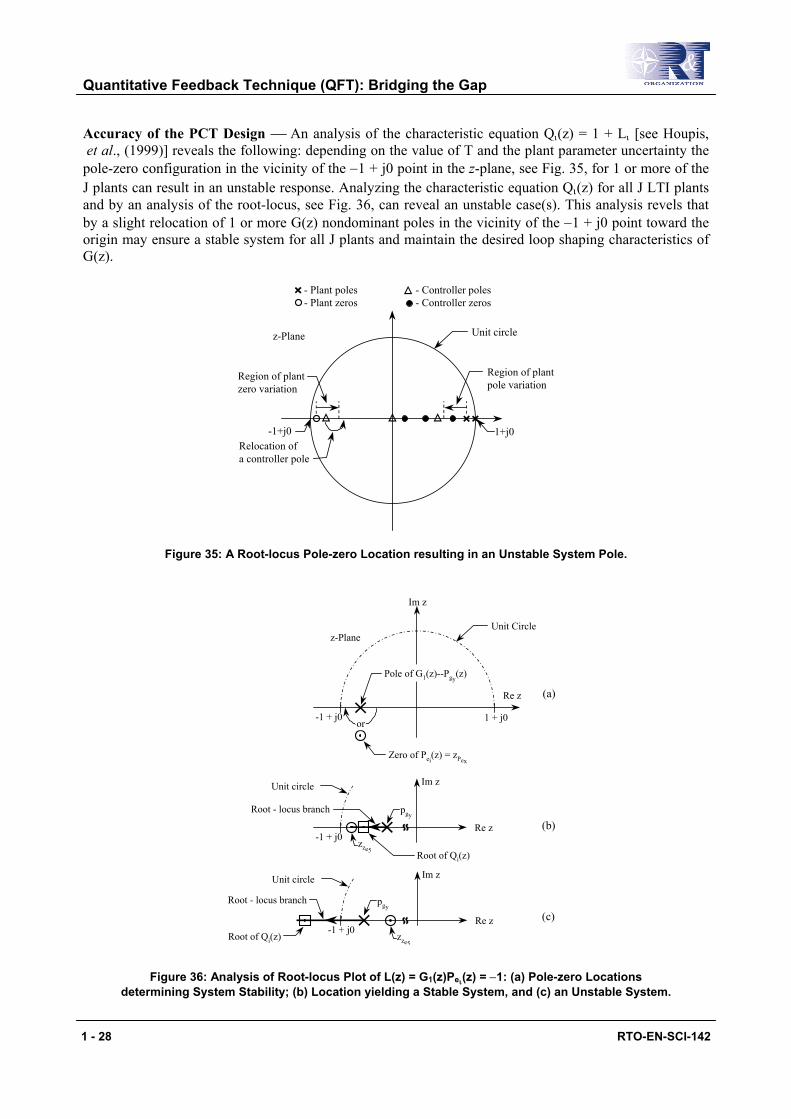
Accuracy of the PCT Design An analysis of the characteristic equation Qι(z) = 1 + Lι [see Houpis, et al., (1999)] reveals the following: depending on the value of T and the plant parameter uncertainty the pole-zero configuration in the vicinity of the −1 + j0 point in the z-plane, see Fig. 35, for 1 or more of the J plants can result in an unstable response. Analyzing the characteristic equation Qι(z) for all J LTI plants and by an analysis of the root-locus, see Fig. 36, can reveal an unstable case(s). This analysis revels that by a slight relocation of 1 or more G(z) nondominant poles in the vicinity of the −1 + j0 point toward the origin may ensure a stable system for all J plants and maintain the desired loop shaping characteristics of G(z).

z-Plane

Region of plantzero variation

Relocation ofa controller pole

Region of plantpole variation

Unit circle

- Plant poles- Plant zeros

- Controller poles- Controller zeros

-1+j0 1+j0

Figure 35: A Root-locus Pole-zero Location resulting in an Unstable System Pole.

z-Plane

Pole of G1(z)--Pgy(z)

Unit Circle

1 + j0

Im z

Re z

-1 + j0or

Zero of Pei(z) = zPex

Im z

Re z-1 + j0

Unit circle

pgy

zze5

Root - locus branch

Root of Qi(z)

Im z

Re z-1 + j0

Unit circle

pgy

zze5

Root - locus branch

Root of Qi(z)

(a)

(b)

(c)

Figure 36: Analysis of Root-locus Plot of L(z) = G1(z)Peι(z) = −1: (a) Pole-zero Locations determining System Stability; (b) Location yielding a Stable System, and (c) an Unstable System.

1 - 28 RTO-EN-SCI-142


Accuracy The CAD package that is used determines the degree of accuracy of the calculations and simulations. The smaller the value of T, the greater the accuracy that can be achieved and it can be enhanced by simulating G(z) and F(z) as cascaded functions, that is:

(62) (Z)G(z)(z)GGG(z) g21 L=

(63) (z)F(z)(z)FFF(z) f21 L=

2.0 MIMO QFT FUNDAMENTALS

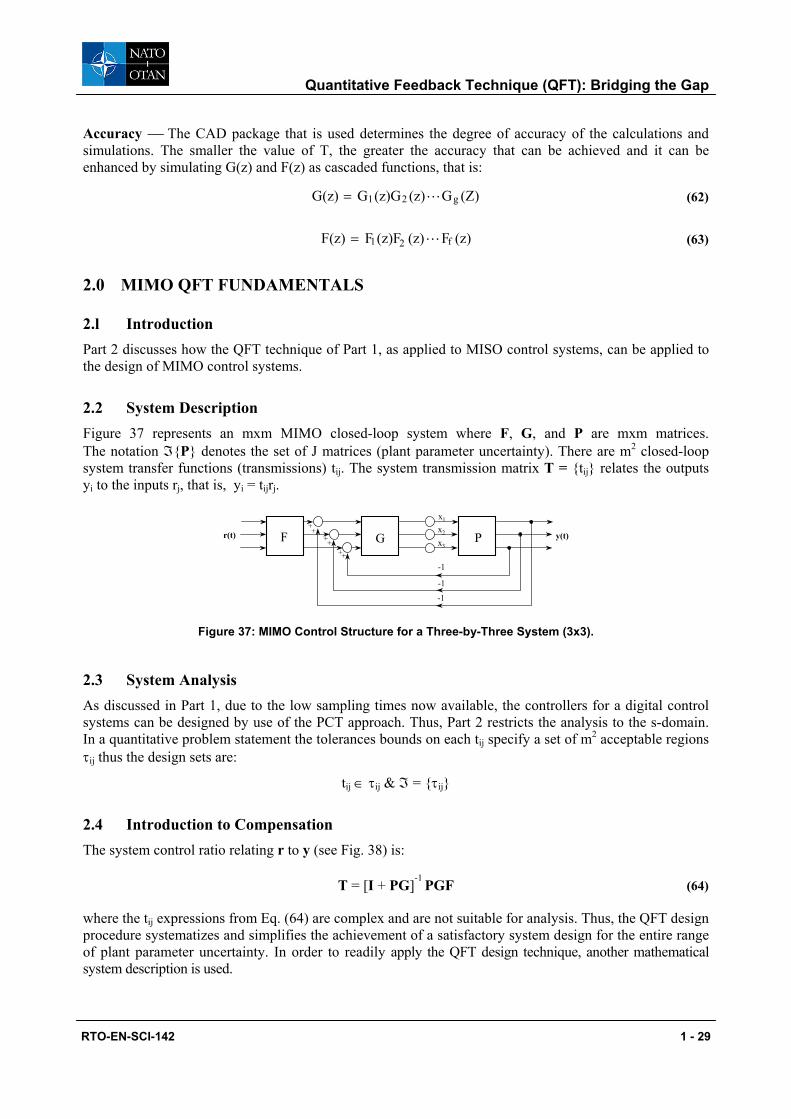
2.l Introduction Part 2 discusses how the QFT technique of Part 1, as applied to MISO control systems, can be applied to the design of MIMO control systems.

2.2 System Description Figure 37 represents an mxm MIMO closed-loop system where F, G, and P are mxm matrices. The notation ℑ{P} denotes the set of J matrices (plant parameter uncertainty). There are m2 closed-loop system transfer functions (transmissions) tij. The system transmission matrix T = {tij} relates the outputs yi to the inputs rj, that is, yi = tijrj.

F G Pr(t) y(t)

-1

-1

++

+

+

+

+

-1

x1

x2

x3

Figure 37: MIMO Control Structure for a Three-by-Three System (3x3).

2.3 System Analysis As discussed in Part 1, due to the low sampling times now available, the controllers for a digital control systems can be designed by use of the PCT approach. Thus, Part 2 restricts the analysis to the s-domain. In a quantitative problem statement the tolerances bounds on each tij specify a set of m2 acceptable regions τij thus the design sets are:

tij ∈ τij & ℑ = {τij}

2.4 Introduction to Compensation The system control ratio relating r to y (see Fig. 38) is:

T = [I + PG]-1 PGF (64)

where the tij expressions from Eq. (64) are complex and are not suitable for analysis. Thus, the QFT design procedure systematizes and simplifies the achievement of a satisfactory system design for the entire range of plant parameter uncertainty. In order to readily apply the QFT design technique, another mathematical system description is used.

RTO-EN-SCI-142 1 - 29


. . .

. . . . . .

. . . . . .

. . . F G P ε P

. . .

v 1 u 1 w 1 y 1 r 1 y m r m v m u m w m

- 1

- 1

Figure 38: A MIMO Feedback Structure.

2.5 Derivation of mxm MISO System Equivalents of a MIMO System

The G, F, P, and P-1 matrices are:

(65) F G

==

mm

2m

1m

m2m1

2221

1211

m

2

1

f.... . .

f...f...

ff......ffff

g.... . . 0...0...

00......g00g

OO

(66)

P

=

mm

2m

1m

m2m1

2221

1211

p.... . .

p...p...

pp......

pppp

O

(67)

p ... pp

. . .

. . .

. . .

p ... pp

p ... p p

=

*mm

*m2

*m1

*2m

*22

*21

*1m

*12

*11

1-

OP

Note that only a diagonal G is considered for this paper although a nondiagonal G allows more design flexibility. The m2 effective plant transfer functions are based upon defining:

P

P

Adj

]det[ = 1/p q

ij

*ijij ≡ (68)

1 - 30 RTO-EN-SCI-142


where the requirement det P be m.p. in order for qij be m.p. The Q matrix is:

(69)

p1/ ... p1/p1/

. . .

. . .

. . .

p1/ ... p1/p1/

p1/ ... p1/p1/

=

q ... qq

. . .

. . .

. . .

q ... qq

q ... qq

=

*mm

*m2

*m1

*2m

*22

*21

*1m

*12

*11

mmm2m1

2m2221

1m1211

OOQ

The inverse plant matrix, P-1, is partitioned to the form:

(70) BP +Λ=== ]q/1[]p[ ij*ij

-1

where Λ is the diagonal part and B is the balance of P-1.

Thus λii= 1/qii = , bii = 0, and for i ≠ j bij = 1 /qij = *

iip *

ijp

Premultipling Eq. (64) by [I + PG] yields:

PGFTPGI =+ ][

Multiplying both sides of this equation by P-1 yields:

[P-1 + G]T = GF (71)

where P is nonsingular. Using Eq. (70) (G diagonal) Eq. (71) is rearranged to the form:

T = [Λ + G]-1[GF − BT] (72)

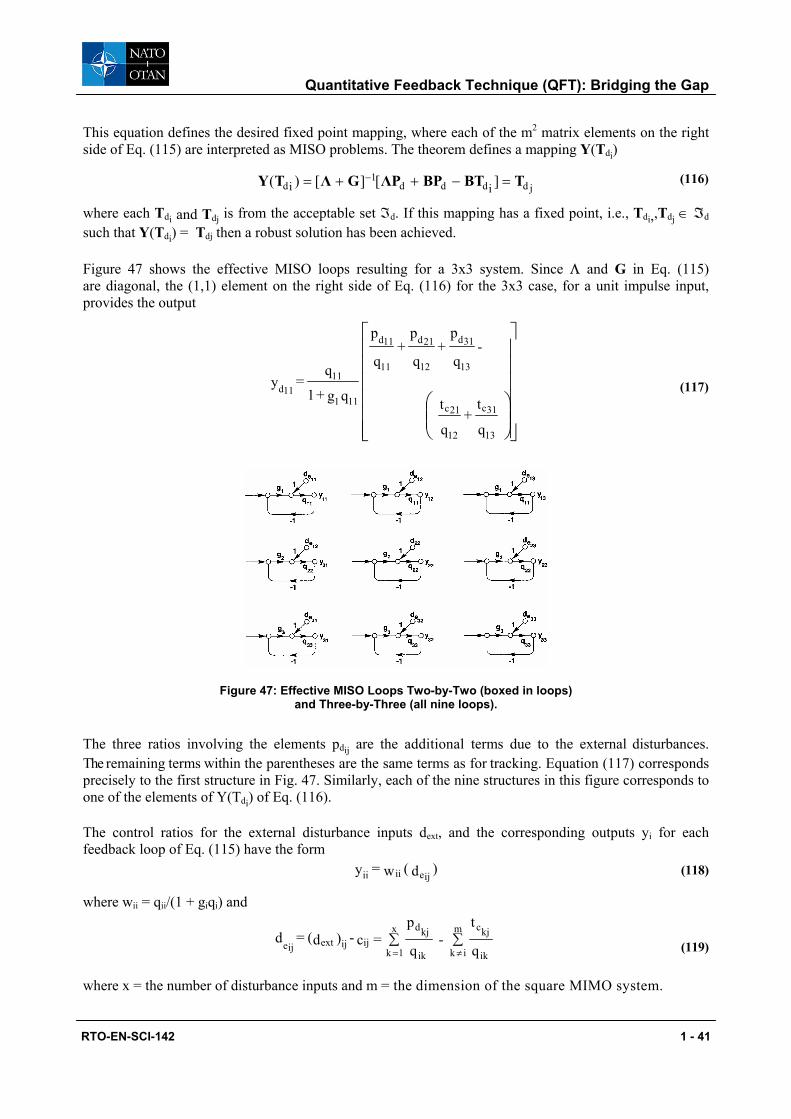
Equation (72) defines the desired Schauder fixed point mapping and where each of the m2 matrix elements on the right side of this equation represents a MISO problem. Thus, the design of each MISO system will yield a satisfactory MIMO design.

Schauder’s fixed point mapping theorem is described by defining a mapping, for a unit impulse forcing function, as follows:

Y(Ti) ≡ [Λ + G]-1[GF - BTi] = Tj (73)

where each Ti and Tj are from the acceptable set T. If the mapping, see Fig. 39, has a fixed point, i.e., Ti,Tj ∈ T such that Y(Ti) = Tj, then a robust solution has been achieved. For a 3x3 case, for a unit impulse input, Eq. (73) yields the output:

qt +

qt - fg

qg + 1

q = y

13

31

12

21111

111

1111 (74)

RTO-EN-SCI-142 1 - 31


Enclosure of all acceptable T∈ℑ

T

Ti

Tj

Y(Ti)

ℑ

Figure 39: Schauder Fixed Point Mapping.

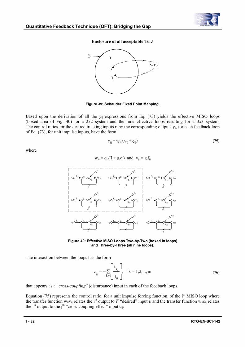
Based upon the derivation of all the yij expressions from Eq. (73) yields the effective MISO loops (boxed area of Fig. 40) for a 2x2 system and the nine effective loops resulting for a 3x3 system. The control ratios for the desired tracking inputs rj by the corresponding outputs yi, for each feedback loop of Eq. (73), for unit impulse inputs, have the form

(75) )c + v(w = y ijijiiij

where

wii = qii/(l + giqi) and vij = gifij

c11

f11 g1r1 y11q11

-1

c13

f13 g1r3 y13q11

-1

c12

f12 g1r2 y12q11

-1

c21

f21 g2r1 y21q22

-1

c23

f23 g2r3 y23q22

-1

c22

f22 g2r2 y22q22

-1

c31

f31 g3r1 y31q33

-1

c33

f33 g3r3 y33q33

-1

c32

f32 g3r2 y32q33

-1

Figure 40: Effective MISO Loops Two-by-Two (boxed in loops) and Three-by-Three (all nine loops).

The interaction between the loops has the form

m1,2,...,k,q

tc

ikik

kjij

=∑−=≠

(76)

that appears as a “cross-coupling” (disturbance) input in each of the feedback loops.

Equation (75) represents the control ratio, for a unit impulse forcing function, of the ith MISO loop where the transfer function wiivij relates the ith output to ith “desired” input ri and the transfer function wiicij relates the ith output to the jth “cross-coupling effect” input cij.

1 - 32 RTO-EN-SCI-142


Transfer Functions The term wiivij relates the “desired” ith output to the jth input rj (see Fig. 40) and where the term wiicij relates the ith output to the jth “cross-coupling” input cij. Thus, the outputs [see Eq. (75)] are now expressed as

Yij = (yij)rj + (yij)cij = yrj + ycij (77)

or, based on a unit impulse input:

Tracking → (78) vw = y = t ijiir jr j

Cross-coupling → (79) cw = y = t ijiicijcij

Object of Design The design objective is that each loop tracks its desired input while minimizing the outputs due to the cross-coupling inputs. Note that each MISO system’s cross-coupling effect input is a function of all other loop outputs.

MISO Control Ratios To achieve the desired MISO control ratios for the nine MISO structures of Fig. 40 requires that the tij must be a member of the acceptable tij ∈ τij and the gi and fij must be chosen to ensure the condition on tij is satisfied. To satisfy these constraints constitutes nine MISO design problems. If all MISO problems are solved a unique solution is achieved for Fig. 37.

2.6 Performance Bounds The developments in this paper are based on the utilization of diagonal G & F matrices, i.e.:

fij = gij = 0 for i ≠ j

In Fig. 40 the tij terms, for i ≠ j, involve only the cross-coupling (disturbance) responses:

yij = wijcij

The tij terms, for i = j, [see Eqs. (77)-(79)] are composed of a desired tracking term tr and an unwanted cross-coupling term tc. The desired tracking specifications are given by the upper and lower bounds of Fig. 41. Whereas the cross-coupling specification for all MISO loops are given by only an upper bound.

a11

RLT

RUTb11

ω

|t11(jω)|

Figure 41: Upper and Lower Tracking Bounds.

Bounds The required specified P.S. bounds are shown in Fig. 41 and 42. The upper bounds , within the BW, is

'iib

(80) 'iiiiiic bb −=τ

RTO-EN-SCI-142 1 - 33


where represents the maximum portion allocated for cross-coupling rejection, where represents

the upper bound for the tracking portion of tii, and where a represents the lower bound for the tracking portion of tii.

iicτ 'iib

ii′

c iiτ

ω

aii

aii ′

bii

′bii

∆τ ∆τRLi

Figure 42: Allocation for Tracking and Cross-coupling Specifications for the tii Responses.

Modified Tracking Specifications Based upon Eqs. (78) - (80) the specifications for the |tii(jω)| responses of Fig. 41 are modified as shown in Fig. 42. The modification is based upon the allocation of δR(jωi) [see Fig. 5b] and the allocated τcii for cross-coupling effect specification. Based upon the specified BW above which the output sensitivity is ignored, synthesize the G and F such that for all P ∈ P:

(81) iiUr11r11Lr11iib = )( |t| )( = a ′≤≤′ ττ

A finite ωh is recommended since in strictly proper systems feedback is not effective in the high frequency range.

2.7 Cross-Coupling (Disturbance) Specification for i ≠ j Only an upper bound is required for the disturbance specification, i.e.:

|tcij| ≤ |bij| (82)

Thus, the synthesis of G(s) and F(s) must satisfy both Eqs. (81) and (82).

2.8 Example: A 2x2 MIMO System The tij control ratios for this 2x2 MIMO system example, from Eq. (75) for unit impulse inputs, are

gq1

qt - fg

= t g + q

1qt - fg

= t :rinput For

g + q1

qt - fg

= t g +

q1

qt - fg

= t :rinput For

222

21

12222

22

111

12

22121

122

222

21

11212

21

111

12

21111

111

+

(83a)

(83b)

1 - 34 RTO-EN-SCI-142

Multiplying the t11 and t12 equations by q11 and the t21 and t22 equations by q22 in Eq. (83), respectively, yield the equations shown in Fig. 43. Associated with each equation, in this figure, are their corresponding SFG.

Figure 43: A 2x2 MISO Structures and their Corresponding tij Equations.

Tracking Bounds The ii tracking bounds are determined in the same manner as for a MISO system; i.e., by the use of templates for the ii loop plant the value of ∆τrii, shown in Fig. 42, are used to satisfy the constraints of Eq. (81).

Cross-coupling Bounds From Eqs. (84) and (86), in Fig. 43, the following cross-coupling transfer functions are obtained:

= ττ c11c ij1

1111c11

1

c = |t| ≤

+ L

q (88)

b = b 1

c = |t| 12ij

1

1112c 12

≤+ L

q (89)

Substituting for c11 and c12 into Eqs. (88) and (89), then replacing t2l and t22 by their respective upper bound values b2l and b22, and then rearranging these equations will yield the following equations:

1121

11c

11

12

1

Mb1

1=≤

+

τ

q

q

L (90)

1222

12

11

Mb

b

1

1 12

1

=≤+ q

q

L (91)

In order to use the N.C. it is necessary to substitute into these equations L1 = l/l1 which results in the following equations:

RTO-EN-SCI-142 1 - 35


121

111

1

1 M1

M1

≤+

≤+ l

l

l

l (92)

These equations permit the determination of the Mm value for each value of ωi over the set J. For example: since L1 = 1/l1 the reciprocal of these Mm(jωi) values, based on l1, yield the values, based on L1 of the corresponding M-contours or the cross-coupling bounds Bc1(jωi) for ω = ωi on the N.C. In order to use a CAD package, Eqs. (90) and (91) are rearranged to

plantsJallovermax11

21

12

111

b

b|1|

−≥+

q

qL

plantsJallovermax12

22

12

111

b

b|1|

−≥+

q

qL

Thus, the largest magnitude of |q11 /q12| over the set J is readily determined by use of the CAD package. This magnitude is inserted into Eqs. (90) and (91) to yield the corresponding cross-coupling bounds on the N.C.

Optimal or Composite Bounds The points on the composite bound, for a given value of ωi, and for a given row of MISO loops of Fig. 40 is the composite of one tracking bound and m cross-coupling bounds for this value of ωi. That is, select the largest dB value, for a given phase angle on the N.C., from all the tracking and cross-coupling bounds for these loops at this value of frequency to be the point on the optimal or composite bound. The MIMO QFT CAD package developed by Sating, (1992) is designed to perform this determination.

2.9 Weighting Matrix

For control systems whose plant matrix Pb has more inputs Vl than outputs Ym a weighting matrix W = {wij}, see Fig. 44, is utilized to obtain an effective square mxm plant matrix Pe, i.e.,

Pe = PbW

where Pb is an mxl matrix and W is an lxm weighting matrix.

W Pb...

.... . .

U 1

U m

V1

Vl

Y1

Ym

Pe Figure 44: An mxm Effective Plant Pe(s).

2.10 QFT Design Methods There are two QFT design methods Method 1 and Method 2. Method 1 involves synthesizing the loop transmission Li and prefilter fii which are independent of the previous synthesized loop transmission and prefilter functions. Whereas, Method 2 involves substituting the synthesized gi and fii of the first (or prior) MISO loop(s) that is (are) designed into the equations that described the remaining loops to be designed. At the onset a decision needs to be made as to the order that the Li functions are to be synthesized. Generally loop i is chosen on the basis of the performance requirements. For example: the loop i having the smallest value of ωϕ is chosen as the first loop to be designed then followed by designing the loop having the next smallest of ωϕ as second loop, etc. This is an important requirement for Method 2.

1 - 36 RTO-EN-SCI-142


Method 1 Method 1 involves over design (worst case scenario). In determining the Mij. values of Eqs. (90) and (91) (2 x 2 case), for each value of ωi, obtain the smallest magnitude of |ql2/q11| (or the largest value of |q11/q12|) in Eqs. (90) and (91) over the entire J LTI plant set. These values are utilized to determine the bounds. This method requires that diagonal dominance condition be met. If this condition is not satisfied Method 2 needs to be used.

Method 2 This method involves selecting the loop i having the smallest phase margin frequency requirement to be designed first. For example, by selecting loop i = 1 results in the synthesis of G1 and f11. These are now known LTI functions which are used to define the loop i = 2 effective control ratio transfer functions. That is, substituting Eq. (84) [t11] into Eq. (85) [t21] and rearranging results in a new expression for t2l in terms of g1 and f11, i.e.:

+

+−=

e222

121

e22111

21qg1

)L(1q

qLf

t (93)

The effective loop 2 transfer function is, by definition:

2112

221112

121

122e22 qq

qqγwhere

)γ(L1

)L(1qq =

−+

+= (94)

Repeating a similar procedure the expression for t22 is:

e222

e2222222

qg1

qgft

+= (95)

Equations (93)-(95) involve known f11 and g1 which reduces the over design of loop 2.

2.11 Synthesizing the Loop Transmission and Prefilter Functions Once the optimal bound, for each ωI have been determined, for each Li loop, then the synthesis procedures of Section 1.2 for determining the loop transmission and prefilters transfer functions are used to determine the gi and the fii for the MIMO system.

3.0 SYSTEM WITH EXTERNAL DISTURBANCE INPUTS

3.1 Introduction The previous sections have dealt with just the tracking problem. This section deals with the regulator problem, i.e.:

Input tracking commands: r(t) = 0

External disturbance input: d(t) = {dk(t)} k = 1,2,...,x

The development of this section permits the design of a robust multivariable control system having both types of inputs. The air-to-air refueling problem is used as the basis for the development of the regulator problem [Trosen, (1993]. An automatic control of the receiving aircraft during aerial refueling operations

RTO-EN-SCI-142 1 - 37


is most beneficial. The results are applicable to any regulator and tracking-regulator problem [Houpis et al., (1999)].

3.2 Problem Statement The design problem is to maintain a precise position of the receiving aircraft (receiver) relative to the tanker in presence of such disturbances as wind gusts, and in changes of mass and moments of inertia (see Fig. 45) and to prevent a disconnect of the refueling boom due to excessive changes in position. The six-degrees-of-freedom (uncontrolled) A/C models are used to develop the required state space models. A set of J = 16 bare A/C plants are used to account for the uncertainty of the C-135B aircraft during an air-to-air refueling. See Houpis et al., (1999) for more details used in the development of these models.

Hinge Point (Tanker)

Receptacle (Receiver)

RZ

XY

Into page

Figure 45: Control Problem Geometry.

3.3 Disturbance Modeling Disturbance models are generated by developing the augmented state-space models of the aircraft in the presence of wind gusts and fuel transfer inputs. The external disturbance inputs are represented by the vector d and contain three disturbance components. These components are:

---- Pitch plane wind induced disturbance Γpitch

---- Lateral channel wind induced disturbance Γlat

---- Refueling disturbance Γrf

The total disturbance modeled is given by:

(96) rfrflatpitchpitch lat= dddΓd Γ+Γ+Γ

The state and output equations are: Cxy Γdu Bx Ax =and + + = & (97)

3.4 Plant and Disturbance Matrices Based on zero initial conditions from Eq. (97) the following equations are obtained:

sX = Ax - Bu - Γd (98)

1 - 38 RTO-EN-SCI-142


x = [sI - A]-1

Bu + [sI - A]-1

Γd (99)

y = Cx = C[sI - A]-1

Bu + C[sI -A]-1

Γd = P(s)u + Pd(s)d (100)

where

P(s) = C[sI - A]-1

B (101a)

Pd(s) = C[sI - A]-1

Γ = {pdij} (101b)

and where the plant model PF is partitioned into the two matrices (see Fig 46) P(s) and Pd(s) where P(s) = Pe(s) for a square plant matrix P(s) and the matrix Pd(s) models the transmission from the external disturbance inputs to the output of PF. If P(s) is not a square matrix then a weighting matrix W(s) is used to yield Pe(s) = P(s)W. Equation (100) is represented in Fig. 46.

r v uG(s) P(s)

Pd(s)

y

PFdext

Figure 46: QFT Compensator with Output External Disturbance.

3.5 MIMO QFT with External Output Disturbance Figure 46 represents an mxm closed-loop system in which F(s), G(s), P(s), and Pd(s) are mxm matrices. Note that P(s) = {P(s)} and Pd(s) = {Pd(s)} are sets of matrices due to the plant and disturbance uncertainties, respectively. The objective is to find a suitable mapping that permits the analysis and synthesis of a control system by a set of equivalent MISO control systems.

Mathematical Development From Fig. 46 the following equations are obtained:

(102) (s) - (s)r (s) (s)(s) (s) (s)(s)(s)(s) = (s) extd yvvGudPuPy ==+

For the regulator case, with zero tracking input:

[ ]0 0, 0, = (t)T

r (103)

From Eqs. (102) and (103), where henceforth the (s) is dropped in the continuing development, obtain the following equations:

(104) Gyuyv - = - =

which yields

(105) extd - = dPPGyy +

Equation (105) is rearranged to yield:

[ ] extd-1

+ = dPPGI y (106)

RTO-EN-SCI-142 1 - 39


Based upon unit impulse disturbance inputs for dext the system control ratio relating dext to y is

[ ] d1-

d + = PPGIT (107)

Pre-multiplying Eq. (107) by [I + PG] yields

[ ] dd + PTPGI = (108)

Pre-multiplying both sides of Eq. (108) by P-1 results in

(109) d1

d1 ] [ PPTGP −− =+

Let

(110)

=−

*mm*m2*m1

*2m*22*21

*1m*12*11

1

ppp

ppp

ppp

L

MMM

L

L

OP

The m2 effective plant transfer functions are formed as

adj

det =

p1

qij

*ij

ijP

P≡ (111)

The Q matrix is then formed as

(112)

==

*mm

*m2

*m1

*2m

*22

*21

*1m

*12

*11

mmm2m1

2m2221

1m1211

1/p1/p1/p

1/p1/p1/p1/p1/p1/p

qqq

qqqqqq

L

MMM

L

L

L

MMM

L

L

Q

where P = [pij], P-1 = [ ] = [1/qij], and Q = [qij] = [1/ ]. The P-1 matrix is partition as follows: *ijp *

ijp

(113) BΛP + = ] q1/ [ = ] p [ ij*ij

1- =

where Λ is the diagonal part of P-1 and B is the balance of P-1. Thus,

λii = l/qii = p , bii = 0, and bij = l/qij = for i ≠ j *ij

*ijp

Substituting Eq. (113) into Eq. (109) with G diagonal, results in

(114) dd + [ = ] + + [ ]PB ΛTGBΛ

Rearranging Eq. (114) produces

(115) }t { = ] - + [] + [ dijddd-1

d = BTBPΛPGΛT

1 - 40 RTO-EN-SCI-142


This equation defines the desired fixed point mapping, where each of the m2 matrix elements on the right side of Eq. (115) are interpreted as MISO problems. The theorem defines a mapping Y(Tdi)

(116) jdddd

1d ][][)( ii TBTBPΛPGΛTY =−++= −

where each Tdi and Tdj is from the acceptable set ℑd. If this mapping has a fixed point, i.e., Tdi,,Tdj ∈ ℑd

such that Y(Tdi) = Tdj then a robust solution has been achieved.

Figure 47 shows the effective MISO loops resulting for a 3x3 system. Since Λ and G in Eq. (115) are diagonal, the (1,1) element on the right side of Eq. (116) for the 3x3 case, for a unit impulse input, provides the output

q

t+

q

t

- q

p +

q

p +

q

p

qg + 1

q = y

13

c31

12

c21

13

d31

12

d21

11

d11

111

11d11

(117)

Figure 47: Effective MISO Loops Two-by-Two (boxed in loops) and Three-by-Three (all nine loops).

The three ratios involving the elements pdij are the additional terms due to the external disturbances. The remaining terms within the parentheses are the same terms as for tracking. Equation (117) corresponds precisely to the first structure in Fig. 47. Similarly, each of the nine structures in this figure corresponds to one of the elements of Y(Tdi) of Eq. (116).

The control ratios for the external disturbance inputs dext, and the corresponding outputs yi for each feedback loop of Eq. (115) have the form (118) ) d (w = y eijiiii

where wii = qii/(1 + giqi) and

- = ∑∑≠=

m

ik ik

kjcx

1k ik

kjdijijexteij q

t

q

pc - )d( = d (119)

where x = the number of disturbance inputs and m = the dimension of the square MIMO system.

RTO-EN-SCI-142 1 - 41


Thus, the interaction term, Eq. (119), not only contains the cross-coupling interaction but also the external disturbances, i.e.:

∑∑≠=

m

ik ik

ijcij

x

1kik

kjdijex q

t= cand

q

p= )d t( (120)

where (dext)ij represents the external disturbance effects and cii represents the cross-coupling effects. The additional equations, quantifying both the external disturbance (dext)ij and the internal cross-coupling effects cij, are derived to utilize the improved method QFT design technique. These equations are used to define the disturbance bounds for subsequent loops based on the completed design of a single loop.

3.6 Tracker/Regulator MIMO Control System A MIMO system, that involves both tracking and external disturbance, can now be designed by either QFT Method 1 or Method 2. In Fig. 48 the cij terms are replaced by the deij terms; that is, Fig. 47 is modified by including the tracking inputs ri ≠ 0. The modified figure now represents the tracking/regulator MIMO control system. The optimal bounds are now a combination of not only the most stringent portion of each of the tracking and cross-coupling effect bounds but also that of the bounds due to the external disturbance (dext)ij of Eq. (120).

c11

f11 g1r1 y11q11

-1

c13

f13 g1r3 y13q11

-1

c12

f12 g1r2 y12q11

-1

c21

f21 g2r1 y21q22

-1

c23

f23 g2r3 y23q22

-1

c22

f22 g2r2 y22q22

-1

c31

f31 g3r1 y31q33

-1

c33

f33 g3r3 y33q33

-1

c32

f32 g3r2 y32q33

-1

Figure 48: Effective MISO Loops Two-by-Two (boxed in loops) and Three-by-Three (all nine).

4.0 NOW THE “PRACTICING ENGINEER TAKES OVER”

4.1 Introduction Scientific Method The scientific method uses mathematical methods to gain insights into, generalize, and to expand the state-of-the-art. This method often requires proof of theorems, corollaries, and lemmas. At this stage, in general, the researcher (a) is not concerned whether his/her efforts result in the solution of “real world problems” which are nonlinear and (b) applies linear analysis and synthesis techniques in the research effort. The scientific method is necessary for the researcher to be able “to see the trees from the forest,” and thus to be able to achieve positive results.

Engineering Method The engineering method, where applicable, is a method where the engineer takes over and applies these new results to real world problems. The engineer is at the “interface” of the real world, and with the body of knowledge and theoretical results available in the technical literature.

Application of the Scientific Method to OFT Professor I. M. Horowitz applied the scientific method in his development of QFT approach to the engineering design of robust control systems [Horowitz, et al.,

1 - 42 RTO-EN-SCI-142


(1973)]. Professors F. Bailey, 0. D. I. Nwokah, et al., also used this approach to enhance the mathematical rigor of QFT and to help the engineer to bridge the “interface” gap in applying the QFT. This body of knowledge must be coupled with the “body of engineering knowledge” pertaining to the application, when dealing with nonlinear systems and real world problems. This requires that the engineer have a good understanding of the physical characteristics of the plant to be controlled.

“Bridging of the Gap” The “Bridging of the Gap” [Houpis, (2002)] is best illustrated by the following anonymous saying:

“In THEORY (Scientist)

There is no difference between THEORY and PRACTICE.

In PRACTICE (Engineer)

There is a difference between PRACTICE and THEORY.”

Conclusion The control system design task is a multi-stage process which entails many steps, say from A to Z. Mathematics is useful in taking the engineer through some of these steps, say from P to S. The engineer should make the required modelling assumptions, hypotheses, and simplifications needed to proceed from A to 0, so that the mathematical problem is tractable and the existing theory can be applied. Finally, the steps T to Z entail extensive simulations where the validity of the model is verified, the implementation issues are addressed, and the design is validated.

4.2 Transparency of QFT There are essentially four elements that provide the “transparency” of the QFT technique and which enhance its ability to design and to solve real world problems [Houpis, et al., (1999)]. These elements are:

Size of Template The width and height of a template, see Fig. 49, play an important role in Bridging the Gap at the onset of the design process. That is, the engineer at the onset of the design process can readily determine whether a fixed compensator G can be synthesized that yields the desired system performance. If only the template height is the problem then the engineer needs to employ straight gain scheduling. When control effector failures need to be accommodated, the width of the template can be excessive and a successful design is not possible [Cacciatore, (1995)]. For this case, the designer needs to either reduce the percentage of failure to be accommodated or to eliminate the effector failure case(s), in order to reduce the width of the template. Chapter 10 by Houpis, et al., (1999) provides an example of how an engineer utilized the knowledge of plant parameters and the performance characteristics and specifications, to select a set of J plants that ensures a template shape which will represent as accurately as possible the extent of plant parameter uncertainty.

Figure 49: A Template Representing J LTI Plants at ω = 30 rad/sec.

RTO-EN-SCI-142 1 - 43


Phase Margin Frequency In order to ensure that the value of the specified phase margin frequency ωφ is not exceeded by any of the plants in the set then:

(a) When all J plants are stable, select the nominal plant pι to be the plant lying at the “top” vertex of the template. This assumes that this plant always lies, for all template frequencies, at the top of the templates. If not, next best use the template for ωφ to select the “top” plant as the nominal.

(b) If one or more plants in the set P are unstable, then the design engineer must select as the nominal plant the plant Pι that has the highest degree of instability (the plant whose unstable pole lies furthest to the right in the s-plane) as the “worst case plant.”

This rule for the selection of the nominal plant facilitates the achievement of the specified value of ωφ. It is advisable that one of the templates, for each loop, be obtained at the respective BW(Lι) frequency.

Signal Flow Graph The signal flow graph (SFG) for the portion of Fig. 50 that represents Pe is helpful in the initial selection of the values of wij of the weighting matrix W [see Eq. (121)] and in modifying some of these values during the simulation phase of the design process.

y = Peu = PWu (121)

PWGF

δar

δer

δry

δTVy

δep

δTVp

δr

δe

δa p

q

r

pcmd

qcmd

rcmd

Pe YR

Figure 50: MIMO QFT Control Structure Block Diagram.

The selection of values, etc., can be further enhanced by the engineer’s firm understanding of the interrelationship of the plant outputs with the inputs to the W matrix.

Minimum Order Controller (MOC) G The implementation of an m-order controller in a digital flight control system (FCS) results in m-time delays. Thus, during the first m-1 time instants the input has a limited effect on the output, for the output is partially determined by the m initial conditions. Thus, the control action is delayed. A factor to be considered in maintaining low-order controllers is that on board flight control computers have a limited capacity due to other non-control related computing requirements. As a rule, about 30% of the computer capacity is allocated to the FCS and 70% for non FCS requirements. To achieve this desideratum some designers, or design methods, have recourse to the plant P, and in-turn Pe by “doctoring” or “padding” by inserting additional poles and/or zeros into P. This results in an “augmented” plant matrix Pes which these designers base their design on in order to achieve a so-called “minimum-order” G. These “additional poles and/or zeros” in reality are poles and zeros of G.

To achieve the MOC G, during the QFT loop shaping phase, the poles and zeros of the nominal plant qiio are used in synthesizing a satisfactory loop shaping transfer function Lio. Doing so, yields the MOC gi = Lio/qiio. Some or all of these elements, or comparable ones, are not available in other, optimization based, multivariable control system design techniques. This minimizes their ability to achieve, in a relatively “short design time,” a design that meets all the performance specifications that are specified at the onset of the initial design effort.

1 - 44 RTO-EN-SCI-142


4.3 Body of Engineering QFT Knowledge Years of applying the QFT robust control design technique to real world nonlinear problems have evolved the following Engineering Rules (E.R.). These rules were developed by Houpis, et al. (1999), and the reader is referred to this text for a more complete presentation. The rules are:

E.R.1 Weighting Matrix The weighting matrix W = {wij} is required to achieve a square equivalent plant matrix. It is desired to know at the onset, if possible, to achieve m.p. qii’s by the proper selection of the wij elements. A m.p. qii plant is most desirable for it allows a full exploration of the “benefits of feedback,” i.e., high gain. By applying the Binet-Cauchy theorem, as shown by Houpis, et al., (1999), it is possible to determine if m.p. qii’s are possible. It may be desirable to obtain complete decoupling for the nominal plant case, i.e.,

(122) PWP =

p 0 0

0 p0

0 0 p

=

mm

22

11

ediag

K

MKMM

K

K

For non-nominal plants complete decoupling, in general, will not occur but the degree of decoupling will have been enhanced. Method 1 is then more readily applicable, with the additional benefit of reduced closed-loop BW.

E.R.2 n.m.p. qii’s For manual flight control systems, if a RHP zero is “close” to the origin (see Fig. 51) it is not necessary deleterious since the pilot will input a new command before the effect of the closed-loop pole, associated with this zero, is noticeable. Assume that the unstable pole is outside the closed loop system’s BW. If this RHP zero is “far out” to the right, outside the BW of concern, in manual control it does not present a problem. For these cases a satisfactory QFT design may be achievable.

σ

jω

S-plane

“Far - Out”

“Close - In”

ε

Figure 51: Right-half-Plane Analysis.

E.R.3 Templates The adage “picture is worth a thousand words” applies to the preliminary task of determining if a robust control solution exists. If theorems, corollaries, and/or lemmas obtained by the scientific method, reveal that no loop shaping solution exists then one must step back and do a “trade-off” in which some specifications are relaxed in order to achieve a solution, or one must be willing to live with a degree of gain scheduling. A graphical analysis can reveal the following:

(a) The maximum template height is too large forcing one or more bound or the composite bound being violated. The engineer needs to decide if gain scheduling is required and if it is feasible in order to yield a design that satisfies all the bounds.

RTO-EN-SCI-142 1 - 45


(b) The analysis may reveal that the templates are too “wide” (magnitude of the phase angle width) thus prohibiting a QFT solution or a solution by any other multivariable design technique. This is true for real-world control problems that involve control effector failures. In these design problems, generally, the worst failure case is the culprit in generating large “angle width.” Thus, in order to achieve a solution it is necessary to relax the requirement that the “worst failure case” be accommodated. It is also necessary to stipulate what failure case or cases a successful design is achievable. In determining the “reasonable failure cases” that can be accommodated by robust (not adaptive) control one must consider if 10%, ... , 80% failure still permits enough control authority! This percentage of failure can only be determined by a individual who is knowledgeable of the physical plant being controlled. A knowledge of the plant (application) “is king” when it comes to the design of a feedback compensator or controller for the given plant.

(c) In Section 10-4 of Houpis, et al. 1999, it is shown how the engineer’s insight into the plant’s physics helps to efficiently determine the boundary of the template (where the parametric uncertainty is represented). A possible method of reducing the size of the templates is given by E.R.8.

E.R.4 Design Techniques For all the design methods the P.S. must be realistic and commensurate with the real world plant being controlled. Situations occurred where a conclusion was reached that no acceptable design was possible. For these situations when one “stepped back” and asked the pertinent question “was something demanded that this plant physically cannot deliver regardless of the control design technique?” It was determined that some or all of the prescribed specifications were unrealistic.

E.R.5 QFT Method 2 − In using Method 2 it is known at the onset the ωφ of the succeeding designed loop is larger than the previously designed loops. Thus, arbitrarily picking the wrong order of the loops to be designed can result in the nonexistence of a solution. This may occur if the solution process is based on satisfying an upper limit of the phase margin frequency ωφ, for each loop. The proper order of loops to be designed by Method 2 is to pick the loops in the order of increasing values of the desired ωφ; i.e., first close loop 1, then loop 2, etc where ωφ1 < ωφ2 < ωφ3 < ... .

E.R.6 Minimum order G To ensure the smallest possible order compensator/controller it is necessary to start the loop shaping process by using the loop’s nominal plant as the starting Lo, i.e., Lo = Lo1 = q11o. The loop shaping process is then started by inserting zeros and poles successively in order to obtain the required loop shape, resulting in:

)p (s)p(s)z (s )z (s)(sL = (s)L

v1

w1o1o −−

−−K

K (123)

Finally, from the synthesized loop shaping function the compensator is obtained, i.e., g1 = [Lo]1/q11o.

E.R.7 Minimum Compensator Gain To minimize the effects of noise, saturation, etc. need to minimize the gain required in each loop i while at same time satisfy the P.S. To achieve this goal, a designer, with a good understanding of the N.C. and a good interactive QFT CAD, can use his “engineering talent” to make use of the “dips” in the composite Boi(jωj) – See Fig. 52. Shaping [Lo]i to pass through the dips, where feasible, ensures achieving the minimum compensator gain that is realistically possible.

1 - 46 RTO-EN-SCI-142


Figure 52: QFT Stability and Composite Bounds.

E.R.8 Basic mxm Plant P Preconditioning Using the unity feedback loops for the mxm MIMO plant P yields an mxm preconditioned plant matrix Pp. The templates ℑPP(jωi), in general can be smaller in size than the templates ℑP(jωi). Thus, the QFT design may be performed utilizing the preconditioned matrix Pp.

E.R.9 Nominal Plant Determination The phase margin angle γ, the gain margin, and ωφ of a feedback control system can be readily determined using the N.C. The QFT design technique affords the robust establishment of these FOM. By choosing the nominal plant to correspond to the maximum dB plant on the ωφi = BW(Li) template ensures that ωφ ≤ BW(Li) for all plants. The achievement of a robustly guaranteed gain margin is accomplished readily by selecting a nominal plant that is uniformly the maximum dB plant for all templates at the top of the template. The achievement of a robustly guaranteed desired γ is accomplished readily by selecting the “left-most” plant on all the templates as the nominal plant. This ensures that the desired γ is robustly achieved.

E.R.10 Simulation Run Time The goodness of the design of the “real-world” manual feedback control problems are judged on a pre-specified planning time horizon beyond which the performance is less important since the human operator will inject new inputs to the system. For example, in many manual flight control scenarios the time horizon is 5 s simulation run time.

E.R.11 Asymptotic Results Asymptotic results by mathematical analysis are not as useful as they seem to be, i.e., for external disturbance yD(∞) = 0. Consider the manual control disturbance rejection case where fast disturbance attenuation is more desirable than total disturbance rejection, i.e., YD(∞) = 0, which entails a very long “settling time.”

E.R.12 Controller Implementation To minimize the computer numerical inaccuracy due to the software implementation of G(z), it is necessary to obtain the software implementation by writing the difference equation for each block in Fig. 53.

RTO-EN-SCI-142 1 - 47


Gc(s) = N(s)D(s) O(s)I(s) Gc(w) = N(w)

D(w) O(w)I(w)

(a) The design compensators

Gc(z) = N(z)D(z) O(z)I(z)

(b) z-domain compensator

G1(z)O1(z)

I(z) Gj(z)Oj(z) = O(z). . .

(c) z-domain J cascaded controllers

Figure 53: s- or w-domain to z-domain Bilinear Transformation: Formulation for the Implementation of the G(z) Controller.

E.R.13 Non-ideal Step Function for Simulation For mathematical analysis of LTI systems ideal step functions are utilized. In the real world, the ideal step functions do not exist. Thus, for a more realistic test in determining a control system’s performance through simulation a ramped-up step function is used as shown in Fig. 54. Use of this type of a realistic forcing function has the tendency to minimize the saturating aspects of the system.

1

0 tr, rise timetime

Figure 54: A Ramped-up Step Function.

4.4 Plant Inversion Given the mx1 output vector y and an mx1 input vector u (see Fig. 55) the LTI plant state equation is:

D(s)y = N(s)u (124)

with D(s) = [dij(s)] and N(s) = [nij(s)] being mxm polynomial matrices in s. The resulting plant matrix P (y = Pu) is

)]s(p[ = det

) (Adj = = ij

1-

D

NDNDP (125)

1 - 48 RTO-EN-SCI-142


Pu 1 u 2

u l

.

.

. . . .

y1

..

.y2

ym

..

.

Figure 55: A MIMO Plant.

The inverse plant is expressed as:

(126) ]q[1/ = ]p[ = ij*ij

-1P

It can be obtained from either Eq. (124), i.e., since u = P-1y,

N

DNDNP det ) (Adj = = 1-1- (127)

or from the state equations, i.e.:

(128) (b) = (a) + = CxyBuAxx&

that describe the nth-order plant, where the matrices A, B, C are nxn, nxm, and mxn, respectively, and which, in turn, yield the following expressions:

(129) BuAICy -1]-[s =

dn

= ]-[s = ij1- BAICP (130)

where nij and d are polynomials of degree l and n, respectively, in s; l < n and d is the characteristic polynomial of A.

For the numerical calculation of P-1 it is much better to use Eq. (127) rather than Eq. (130). This is best illustrated by considering a 2x2 (m = 2) plant utilizing the second approach. Thus, from Eq. (130):

}{ndet d

}{n Adjd =

d}/{ndet

}/d{n Adj =

d}/{ndet

dn

Adj

= ij

ij2

2ij

ij2

ij

ij

1-

P (131)

In general, for the mxm control system:

}{ndet d

}{n Adj d =

ij1-m

ijm

1-P (132)

Thus, if P-1 is obtained from Eq. (132), rather than directly from Eq. (127), then m−1 cancellations of the polynomials from the numerator in Eq. (132) with the m−1 polynomials in its denominator is required. The numerical poles/zeros cancellations are not exact due to the inevitable computer round-off. The m−1 such cancellations of each zero of the numerator with the m−1 poles of the denominator must occur. Thus, in order to recover numerical accuracy one must factor all the numerator and denominator polynomials of P-1 and then check out the inevitable inexact cancellations as demonstrated in Fig. 56.

RTO-EN-SCI-142 1 - 49


Roots of High Precision Polynomial (Mathematica).

Roots of Standard Precision Polynomial (MATRIXX, Control-C, MATLAB, Macsyma).

Figure 56: Figures by Sating, (1992).

5.0 APPLICATIONS

5.1 MIMO QFT Example Design Problem A 2x2 analog flight control system (see boxed in loops of Fig. 40) illustrates the increased accuracy and the efficiency achieved by use of the MIMO QFT CAD package developed by Sating, (1992). This CAD package is a straight forward method for designing an analog or discrete MIMO control system. The original design was done by Arnold, (1984) but was redesigned by Sating utilizing his CAD package [Sating, (1992)]. The specifications are: to design a robust analog aircraft flight control system, provide the required stability, and to satisfy the time domain performance requirements. Four flight conditions (Table 4) and six aircraft failure modes (Table 5) are specified. Table 6 lists the resulting set of 24 plant cases that incorporate these flight conditions and failure modes.

1 - 50 RTO-EN-SCI-142

Table 4: Flight Conditions

Flight Condition Aircraft Parameters Mach Altitude

1 0.2 30 2 0.6 30,000 3 0.9 20,000 4 1.6 30,000

Table 5: Failure Modes

Failure Mode Failure Condition 1 Healthy aircraft 2 One horizontal tail fails 3 One flaperon fails

4 One horizontal tail and one flaperon fail: same side

5 One horizontal tail and one flaperon fail: opposite sides

6 Both flaperons fail

Table 6: Plant Models

Flight Condition Failure Mode 1 2 3 4

1 #1 #7 #13 #19 2 #2 #8 #14 #20 3 #3 #9 #15 #21 4 #4 #10 #16 #22 5 #5 #11 #17 #23 6 #6 #12 #18 #24

The P.S. are to design for a stability of γ = 45° phase margin for each of the two feedback loops. The frequency domain performance specifications, when met, result in the desired closed loop system performance in the time domain and are shown as dashed lines on the Bode plots of Fig. 57.

Figure 57: The 2x2 System Performance:

the Specified Performance Bounds in Dashes and tij Responses.

RTO-EN-SCI-142 1 - 51


Design Process The specifications, plant models for the 24 cases, and the weighting matrix, W, are entered into the QFT CAD. If the plant matrix P is not square then an effective square plant matrix Pe = PW is obtained in order to obtain a QFT design. Automated features accessed through the designer CAD interface result in synthesizing the compensators g1(s) and g2(s). The nominal loop transmission functions L1o(s) = g

1(s)q11o(s) and L2o(s) = g2(s)q22o(s) are synthesized (or shaped) so that they satisfy their

respective stability bounds and their respective optimal bounds B1o(jωi) and B2o(jωi). Note that q11o and q22o are the nominal plant transfer functions.

Validation Check A first step in the validation process is to obtain plots of the loop transmission functions L2ι(s), where ι = 1, ... , 24, for all 24 cases on the N.C. These plots are obtained by a CAD routine, see Fig. 58, for the purpose of a stability check. Note, that all the plants are minimum-phase. None of the cases violate the ML stability contour to accept the consequences of violating the disturbance bound for ω = 2 r/s. With L1o(s) and L2o(s) synthesized, the CAD package's automated features expedite the design of the prefilters f11(s) and f22(s).

Figure 58: NC Stability Validation Check of the L2ι(jω) Plots: 24 Open-loop Transmissions.

1 - 52 RTO-EN-SCI-142


As a second step in the design validation process the 2x2 array of Bode plots, shown in Fig. 57, are generated showing on each plot the 24 possible closed loop transmissions from an input to an output of the completed designed system. The consequence of violating the channel 2 disturbance bound, for ω = 2 r/s, is seen where the closed loop transmissions violate the bound b21. This bound is denoted by a dashed line. Beginning at about ω = 2 r/s a violation of the performance bounds during loop shaping may result in violation of the performance specifications for the closed loop system. There is a violation of the b11 bound of Channel 1. The penetration of the upper tracking bound at ωi ≈ 0.1 r/s is due to the phugoid mode which is not a problem; i.e., does not affect the P.S.

Final Check Figure 57 shows a robust design has been achieved for this 2x2 MIMO analog flight control system. The time domain results, although not drawn, meet all performance specifications.

5.2 Other Examples The following is a list of other QFT designed examples that are mentioned by Houpis, et al. (1999): QFT And Robust Process Control, Idle Speed Control For Automotive Fuel Injected Engine, Welding Control Systems, Control System For An Actuator Plant, VISTA F-16 Flight Control System (Including Configuration Variation), Design Of Flight Control Laws For Aircraft With Flexible Wings Using Quantitative Feedback Theory, Robot Controllers, and Wastewater Treatment Control System.

6.0 SUMMARY

The engineers are applying the results of the scientific method to achieving solutions for the 21st century real world problems. The QFT approach has the advantage that it is close to the engineers’ existing experience in conventional (classical) design methods. It also provides the facilities to deal with structured and unstructured parametric uncertainty which appear not to be available in traditional methods. QFT has the attractive features of providing a link with existing techniques whilst at the same time providing many of the advanced features that are needed for the 21st century high performance systems.

The QFT Control System Design Process typifies the “Bridging the Gap” (Houpis, 2002). As an example, a real-world QFT robust multivariable control system design problem for an Unmanned Research Vehicle (URV) is presented by Houpis, et al. (1999) which involves the elements in “Bridging the Gap” as indicated in Fig. 59. Note that at each step of the design process, as denoted by the rectangular boxes, the engineer can ascertain if the P.S. are still being satisfied. If not, as indicated by the curve line emanating from each box that terminates on the “Redesign” box the engineer does not have to complete the entire design process before needing to do a “redesign.”

RTO-EN-SCI-142 1 - 53


Successful Control Design

Dynamics ModelMathematical modelof the system to becontrolled.

Performance SpecificationsThese are the mathematical expressions which represent the functional requirements.

Functional RequirementsThis is the problem statement.Included are the operational goals of the controlled system and its operating environment

QFT Control System DesignProduces control algorithms fortest and implementation

Linear SimulationImplement and test candidate controlalgorithm using Simplified Dynamics

Nonlinear Simulation•Nonlinear Functions•Nonlinear Dynamics

Engineering Interactive Simulation•User supplies commands and then can react to resulting dynamic behavior•Gives a better understanding of control system operation

System TestTryout of controlled system under actual operating conditions

Engineering VisualizationUsed to better understand results of simulations and System tests

Control Authority AllocationAlgorithm to optimize the use of control effectors for efficiency and decoupling

Hardware-in-the-Loop Simulation/Implementation•Real-time operation of control algorithm•Noise corrupted measurements availablefor feedback•Computation cycle time/Sampling Rate•Quantization Error, Warping

Human-in-the-Loop Simulation•Visual cues•Moving base

Templates

Concurrent BodePlots, open and

closed-loop

Robust Stability, performance,and disturbance boundaries as a

function of frequency

Ability to manipulateclosed-loop response as a

function of frequency

Concurrent Nichols Plots

Design can be brokendown by open or closed-loop operating condition

Redesign

Imbedded PerformanceSpecifications

Figure 59: The QFT Control System Design Process: Bridging the Gap.

1 - 54 RTO-EN-SCI-142


7.0 REFERENCES

Arnold, P. B. (1984). Flight Control System Reconfiguration Using Quantitative Feedback Theory. M.S. Thesis, AFIT/GE/ENG/84D-15, School of Engineering, Air Force Institute of Technology, Wright-Patterson, AFB, OH.

Cacciatore, V. J. (1995). A Quantitative Feedback Theory FCG Design for the Subsonic Envelope of the VISTA F-16 Including Configuration Variation and Aerodynamic Control Effector Failures. MS Thesis, AFIT/GE/ENG/95D-04, Graduate School of Engineering, Air Force Institute of Technology, Wright-Patterson AFB, OH.

Horowitz, I. M, and M. Sidi (1973). Synthesis of Feedback Systems with Large Plant Ignorance for Prescribed Time Domain Tolerances. Int. J. of Control, Vol. 16, pp. 287-309.

Horowitz, I. M. (1991). Survey of Quantitative Feedback Theory (QFT). Int. J. of Control, Vol. 53, No. 2, pp. 255-291, 1991.

Houpis, C. H. and G. Lamont (1992). Digital Control Systems: Theory, Hardware, Software. McGraw-Hill, New York, NY, 2nd Ed.

Houpis, C. H. and S. J. Rasmussen (1999). Quantitative Feedback Theory Fundamentals and Applications. Marcel Dekker, New York, NY.

Houpis, C. H. (2002). Horowitz: Bridging the Gap. Int. J. Control, Vol. 12, pp. 295-302.

Phillips, S., M. Pachter, and C. H. Houpis (1995). A QFT Subsonic Envelope Flight Control System Design. National Aerospace Electronics Conference (NAECON), Dayton, OH.

Sating, R. R. (1992). Development of an Analog MIMO Quantitative Feedback Theory (QFT) CAD Package. MS Thesis, AFIT/GE/ENG/92J-04, Graduate School of Engineering, Air Force Institute of Technology, Wright Patterson AFB, OH.

Trosen, D. W. (1993). Development of an Prototype Refueling Automatic Flight Control System Using Quantitative Feedback Theory. MS Thesis, AFIT/GE/ENG/93-J-03, Graduate School of Engineering, Air Force Institute of Technology, Wright-Patterson AFB, OH.

RTO-EN-SCI-142 1 - 55


1 - 56 RTO-EN-SCI-142

Date post:	06-Mar-2018
Category:	Documents
Upload:	dodang
View:	242 times
Download:	1 times

Quantitative Feedback Technique (QFT): Bridging the · PDF fileQuantitative Feedback Technique...

Documents